Cognitive biases, linguistic universals, and constraint-based grammar learningI

Jennifer Culbertsona,b,∗, Paul Smolenskyb, Colin Wilsonb

aLinguistics Program, Department of English, George Mason University, Fairfax, VA 22030, USAbCognitive Science Department, Johns Hopkins University, Baltimore, MD 21218, USA

Abstract

According to classical arguments, language learning is both facilitated and constrained by cognitive biases.These biases are reflected in linguistic typology—the distribution of linguistic patterns across the world’slanguages—and can be probed with artificial grammar experiments on child and adult learners. Beginningwith a widely successful approach to typology (Optimality Theory), and adapting techniques from compu-tational approaches to statistical learning, we develop a Bayesian model of cognitive biases and show thatit accounts for the detailed pattern of results of artificial grammar experiments on noun-phrase word order(Culbertson, Smolensky & Legendre, 2012). Our proposal has several novel properties that distinguish itfrom prior work in the domains of linguistic theory, computational cognitive science, and machine learning.The paper illustrates how ideas from these domains can be synthesized into a model of language learning inwhich biases range in strength from hard (absolute) to soft (statistical), and in which language-specific anddomain-general biases combine to account for data from the macro-level scale of typological distribution tothe micro-level scale of learning by individuals.

Keywords: Bayesian modeling, Optimality Theory, learning biases, artificial language learning, typology,word order

1. Introduction

What are the capabilities and limitations of human language learning? According to classical argumentsfrom linguistics and the theory of learning, answering this question involves discovering the biases of humanlanguage learners. We propose here a formal model of such biases—set within an existing constraint-basedtheory of linguistic typology—and apply it to experimental results that connect laboratory language learningwith recurring word-order patterns across the world’s languages. Our model implements the hypothesisthat learners use Bayesian inference to acquire a grammar under the influence of a set of hard (absolute)and soft (statistical) biases; we focus primarily on the soft biases, as their form and implementation arenovel. The complete set of biases acts as a prior probability distribution for language learning, accountingfor statistical structure that has been observed in linguistic typology and in the performance of individuallearners. Components of the prior that are language-specific, and others that are plausibly cognition-general,are combined by the simple mathematical operation of multiplication.

1.1. Learning biases and typological asymmetriesA central hypothesis of generative linguistic theory is that human learners bring specialized knowledge

to the task of acquiring a language. By restricting the space of hypotheses a learner will entertain, this prior

IThe authors would like to thank Géraldine Legendre, Don Mathis, Mark Johnson, John Hale and five anonymous reviewers forhelpful comments and discussion.∗Corresponding Author: Linguistics Program, George Mason University, 4400 University Drive, Fairfax, VA 22030, USA., Tel:

(703) 993-1160, Fax: (703) 993-1161, Email: jculber4@gmu.edu.

Preprint submitted to Cognitive Science October 29, 2012

knowledge is argued to solve the poverty-of-the-stimulus problem, allowing robust language acquisitionfrom variable and impoverished input (Chomsky, 1965, 1980; although see Pullum & Scholz, 2002).

Striking asymmetries in the frequencies which which different linguistic patterns occur in the world’slanguages constitute a central body of evidence for the cognitive biases operative in language acquisition.Since language learners have prior assumptions about how linguistic systems are structured, it stands toreason that systems that conform better to those expectations will arise more often, and survive longer, thanother systems. Accounting for typological asymmetries has been the explicit goal of generative linguisticswork within the classical framework of Principles and Parameters (e.g. Chomsky, 1986; Baker, 2001) and,as discussed further below, within the more recent constraint-based framework of Optimality Theory (Prince& Smolensky, 1993/2004).

An illustrative example, which provides the foundation for the case study developed here, is a gener-alization about word order in the nominal domain known as Universal 18 (Greenberg, 1963).1 Accordingto Greenberg’s Universal 18, placement of numerals (Num) after the noun (N) asymmetrically implies thatadjectives (Adj) must also be post-nominal (N-Num → N-Adj). A language violating this generalizationwould express ‘two trees’ as trees two but ‘green trees’ as green trees.2 Greenberg’s original sample of 30languages did not contain even one instance of the prohibited pattern, whence the claim that the generaliza-tion is a ‘Universal’ of language. A modern, much larger sample reveals that some languages do feature theprohibited Adj-N, Num-N order. But this order is nevertheless significantly rarer than the other three possi-bilities, accounting for only 4% of attested languages (see Table 1, where the prohibited order is designated‘L4’; Dryer, 2008a,b).

Table 1: Sample of languages from WALS illustrating preference for consistent ordering and sub-preference among inconsistentorder patterns for N-Adj, N-Num over Adj-N, N-Num (shaded). The labels L1, L2, L3, L4 are used throughout the article for thedifferent language types. English, for example, is a type-1 (or ‘L1’) language.

Adj-N N-AdjNum-N 27% (L1) 17% (L3)N-Num 4% (L4) 52% (L2)

Typological data of the type illustrated by Table 1 pose a major dilemma, heretofore unresolved, forgenerative linguistics. It is straightforward to define a set of OT constraints that make L4 an unlearnablepattern, incorrectly predicting that it should not appear in any attested language (see section 2.1). It is alsostraightforward to define a constraint set that grants L4 the same status as the other three languages, failingto predict that it is much less frequent than the others typologically. The dilemma lies in attempting toaccount for the finding that L4 is possible but rare. This is a statistical finding, a soft universal of language,but generative linguistic theories have previously succeeded in accounting for absolute universals only. Notethat the problem is not restricted to constraint-based theories, but applies also to the classical Principles andParameters approach and its contemporary versions (e.g., Chomsky 1981b; Travis 1989; Kayne 1994; Baker2001; Cinque 2005; Newmeyer 2010).

Further inspection of the nominal typology, and of similar cross-linguistic tabulations, reveals that thedilemma surrounding ‘Universal 18’ is far from an isolated problem. Table 1 provides evidence for an-

1A great number of universals have been documented by linguists: see for example the on-line Universals Archive (Plank &Filimonova, 2000), which contains 2029 universals at the time of writing. Implicational universals, like Greenberg’s Universal18, of the form "If a language has x, then it will have y" are of particular interest. The majority of these have been shown to bestatistical (Bickel, 2007; Evans & Levinson, 2009), and thus are often called generalizations rather than universals. Quite a few,like Universal 18, are stated such that of four logically possible linguistic patterns, three are well-attested and the fourth is rare (e.g.the Final-Over-Final constraint, Biberauer, Holmberg & Roberts, to appear).

2Several possible explanations exist as to why Universal 18 holds; these are discussed at length in Culbertson et al. (2012).

2

other well-documented cross-linguistic asymmetry: namely, that languages tend to use consistent orderingof heads relative to their complements (Chomsky, 1981a; Travis, 1984; Baker, 2001). In particular, systemsL2 (N-Num, N-Adj) and L1 (Num-N, Adj-N) together account for 79% of attested languages. A constraintor parameter set that allows only those systems will fail to provide learnable grammars for the remaining21% of languages; a set that allows all four patterns would seem to have nothing to say about the typolog-ical asymmetry between consistent and inconsistent systems. In addition, post-nominal placement of bothNum and Adj (L2) is slightly more frequent than all other patterns combined (52%) —another statisticalgeneralization that must be lost in a theory with absolute biases only.

To preview our proposed solution, we believe that the problem of possible-but-rare languages disappearsunder a probabilistic approach to cognitive learning biases, and that previous research in machine learningand computational cognitive science lays much of the groundwork needed to construct a model of soft biases.However, formally stating the probabilistic biases in a simple, effective manner is a non-trivial matter thatwe take up in the body of the paper. The main idea that we explore with respect to asymmetries in nominalword-order and similar typological patterns is stated in (1).

(1) Con(straint) Biasa. The constraint set available to learners is sufficiently rich to generate all attested languages, butb. there are soft biases that penalize the grammatical use of particular constraints (e.g., the con-

straint that is responsible for Num occurring after N in L4).

In our proposal, the language-specific Con Bias is combined with a well-established and plausiblydomain-general bias discussed below that favors lower-entropy distributions (the Regularization Bias) toform the probabilistic prior for language learning.

1.2. Converging evidence for learning biasesWe pause at this point to address a concern that typological asymmetries are a somewhat indirect source

of evidence for language learning biases. The indirectness is due to the fact that typological distributionshave to a certain extent been influenced by non-cognitive, diachronic factors, such as lineage-specific trends(e.g. Dunn, Greenhill, Levinson & Gray, 2011) and historical or geographic factors that influence howlinguistic patterns spread and change (e.g. Dryer, 2012). Precisely which typological asymmetries shouldbe accounted for within cognitive theory proper is therefore not completely clear from cross-linguistic dataalone.

It would be desirable to obtain converging evidence for the learning biases from first-language acquisi-tion by children, but the complexity of natural input and absence of experimental control makes this difficult.Fortunately, a number of studies have shown that artificial (or ‘miniature’) language learning by adults—which can be done under carefully controlled laboratory conditions—reveals biases that align with typo-logical asymmetries (e.g. Pycha, Nowak, Shin & Shosted, 2003; Wilson, 2006; Finley & Badecker, 2008;Moreton, 2008; St. Clair, Monaghan & Ramscar, 2009, and many others) (see Culbertson, 2012; Moreton& Pater, to appear, for reviews of recent literature on this topic).

One such study, previously reported in Culbertson et al. (2012), provides converging evidence for biaseson nominal word order. During training learners saw pictures of novel objects, and heard phrases describingthem which were uttered by an "informant" and comprised of either an adjective and a noun or a numeraland a noun. The order used by the informant in any particular description depended on the learner’s trainingcondition—corresponding to one of the four patterns in Table 1 (the ‘dominant’ pattern), accompanied bysome variation. At test, learners were asked to produce descriptions of pictures using these two-word phrasetypes.

In this particular study, learners’ reaction to the variation in each condition provides the measure ofbiases by exploiting a general finding in human learning of probabilistic regularities: under certain cir-cumstances, learners will reduce probabilistic variation (e.g. Weir, 1972; Hudson Kam & Newport, 2009;

3

Reali & Griffiths, 2009). This phenomenon has been called regularization.3 Both this general cognitivebias disfavoring variability and the linguistic biases based on the typology in Table 1 were hypothesized toaffect learners’ behavior. In particular, if the dominant ordering pattern in the input conformed to a learner’slinguistic biases, it was expected to be acquired and regularized. On the other hand, if the dominant pat-tern went against a learner’s biases it was expected to be less likely to be acquired veridically (much lessregularized).

The results from the testing phase, illustrated in Fig. 1, mirror the typology: when the dominant trainingpattern used consistent head ordering (conditions 1, 2) learners regularized robustly. Significantly less reg-ularization was found in condition 3, where the inconsistent pattern (N-Adj, Num-N) was dominant in thetraining. Crucially, learners did not regularize when the dominant pattern was the typologically rare (Adj-N,N-Num). As is clear from Fig. 1, differences among the conditions were driven mainly by differences inthe use of Num majority order, with condition 4 significantly under-producing N-Num order. We will showbelow that our proposal accounts for the qualitative and quantitative findings of this experiment, in additionto providing the foundation for an explanation of the typological pattern discussed above.

1 2 3 4

Condition

Pro

babi

lity

of M

ajor

ity O

rder

0.5

0.6

0.7

0.8

0.9

1.0

AdjNumMean

Figure 1: Probability of dominant input order use reported in Culbertson et al. (2012). Bars show, for each condition, probabilityof dominant order for phrases with adjectives, phrases with numerals, and the mean. The solid line at 0.7 indicates the probabilityof the dominant order used in the input.

1.3. Outline

The rest of the paper is organized as follows. We first introduce non-probabilistic approaches to typol-ogy, focusing on Optimality Theory (‘OT’, section 2). We then show how OT can be adapted to account forlanguage-internal and typological patterns that are stochastic rather than absolute (section 2.2). Language-internal stochasticity results from converting grammatical scores to probabilities in a way that is formally

3This notion of regularization should be distinguished from the term ‘regularization’ as used in machine learning literature. Inthe latter context regularization refers to the practice of introducing some prior information in order to, for example, prevent over-fitting. This practice has been justified as essentially imposing Occam’s razor, and in fact in some cases imposes an expectation ofuniformity, or maximum entropy, whereas our regularization bias favors minimum entropy.

4

equivalent to the maximum entropy (log-linear) models widely used in computational linguistics. Account-ing for gradient typological asymmetries—and artificial-grammar results that mirror them—is the role ofthe prior distribution, which we express as a product of weighted factors (section 3). We highlight severalrespects in which our proposal differs from previous work in computational cognitive science and machinelearning, and from related work on typological asymmetries within linguistic theory. Holding the Con Biasconstant, we propose (and evaluate) two possible formulations of the Regularization Bias. Given a space ofprobabilistic grammars and a prior distribution on that space, language learning is formalized as Bayesianinference (section 4). With a small number of fit prior parameters, our model yields predictions that matchthe main experimental results and an independent replication (section 5). In the final section, we summarizeour proposal, results and conclusions (section 6).

2. Linguistic theories of typology

The ways in which languages vary, and limits on cross-linguistic variation, are central topics in descrip-tive and theoretical linguistics. Within generative linguistics, discovering limitations on variation has beentaken to be central to understanding language acquisition. It is well-known that children generalize be-yond their language input, and that all generalizing learning systems must have biases of some form (Gold,1967; Mitchell, 1980). A simple type of bias in the linguistic domain is an absolute prohibition on certainlogically-possible patterns. Therefore, a linguistic theory that prohibits typologically unattested patterns canbe viewed as a statement of the (implicit) biases that make language acquisition possible.

To illustrate the typical generative linguistics approach to typology, below we develop a theory thatpermits all possible orders of Num and Adj with respect to N except for the typologically rare pattern thatcontravenes Greenberg’s Universal 18 (i.e., L4 in Table 1). This theory of nominal word-order will ulti-mately be relaxed to a soft (statistical) theory, as anticipated in section 1. Formulating the absolute versionis worthwhile because it is representative of many theories in the generative literature, it provides grammarsfor the vast majority (96%) of systems in the survey, and it exposes substantive and formal properties thatmust be present in any approach to nominal word-order. By beginning with the idealized, absolute theorywe can identify exactly which aspects of the data remain to be accounted for by statistical softening.

Recall that the great majority of systems in the typology place Num and Adj on the same side of N(i.e., L1: Num-N, Adj-N and L2: N-Num, N-Adj). This fact taken by itself fits comfortably with a highlyinfluential view of typology in generative linguistics, known as Principles and Parameters (P&P; Chom-sky, 1981a, 1986, 1998; Baker, 2001). According to P&P, uniformity across languages results from a setof universal grammar principles, and constrained variation arises from a set of variables or ‘parameters’appearing in those principles. Each possible combination of parameter values determines a language type,and these types collectively exhaust the languages that are predicted to be possible. The principles and pa-rameters together serve as a constraining framework for acquisition, with the learner’s problem reduced tothat of identifying language-specific parameter settings. The locus of language-specificity in this case is theHead Directionality Parameter (Chomsky, 1981a; Travis, 1984), which can be set so that all syntactic headsprecede their complements (as in L1) or all syntactic heads follow their complements (as in L2).4

The Head Directionality Parameter expresses an important generalization about the typology—nominalheads and complements are consistently ordered in nearly 80% of the languages surveyed—but by itself itprovides no grammar for L3 (Num-N, N-Adj). Generative theories have various mechanisms for solvingproblems of this sort, all of which ensure that a general condition (e.g., syntactic heads must precede theircomplements) can be overridden by a more specific one (e.g., the head of an Adj phrase must follow its

4Here we call Adj and Num heads (following e.g. Cinque, 2005), however this is essentially a simple expository expedience; notheoretical significance is attached to the term for present purposes as the work here deals in surface word strings only.

5

complement). For example, consistent ordering may hold at an early stage in the syntactic derivation, withconsistency disrupted by subsequent syntactic movements that target specific heads or complements (e.g. asin Travis, 1989; Cinque, 2005). Alternatively, the grammatical structures of a language can be defined bythe resolution of conflict among conditions (or constraints) of different strengths, as in Optimality Theory.Under this approach, a weaker general constraint can be violated at all stages of syntactic derivation if thereis a stronger specific constraint with which it conflicts.

Constraint-based theories of linguistic typology have proved successful in many empirical domains5,and have lead to a renewed interest in formal models of language acquisition within generative linguistics.We show below that these hard approaches to typology also provide a rather direct route to a probabilisticmodel of grammars and grammar learning. For these reasons, in addition to our own areas of expertise, wefocus on constraint-based theories in the remainder of the paper, beginning with OT.

2.1. Optimality Theory

OT shares with Principles & Parameters the commitment to a universal set of primitives from whichall grammars are constructed. The primitives of OT are members of a universal constraint set (Con). Alanguage-specific grammar is a strict priority ranking of these universal constraints. The hard typologypredicted by a constraint set is determined by all possible priority rankings; if there is no priority ranking ofthe universal constraints that yields a logically-possible system, that system is predicted to be impossible.

To analyze nominal word-order, we provisionally adopt the constraint set in (2).6

(2) Con for nominal word-order (provisional)a. HEAD-L: order all heads to the left of their complementsb. HEAD-R: order all heads to the right of their complementsc. NUM-L: order numeral heads to the left of their complements

The effects of the Head Directionality Parameter discussed earlier can be replicated by ranking a generalconstraint, either HEAD-L or HEAD-R, above the other constraints. The ranking [HEAD-L � HEAD-R,NUM-L] places both Num and Adj before N, while the ranking [HEAD-R � HEAD-L, NUM-L] placesboth Num and Adj after N. The latter case illustrates the central claim of OT that constraint ranking is strict.This ranking determines that the order N-Num is grammatical—in spite of the fact that placing Num afterN violates both HEAD-L and NUM-L— because the alternative order violates HEAD-R, which takes strictpriority over the lower-ranked constraints. A grammaticality calculation of this sort can be convenientlysummarized with an OT tableau, as shown in (3).

(3) Deriving NUM order in L2

5The majority of this work has been in the domain of phonology, however examples in syntax include Legendre, Raymond &Smolensky (1993); Grimshaw (1997); Nagy & Heap (1998); Vogel (2002); Samek-Lodovici (2005); Steddy & Samek-Lodovici(2011); Pater (2011); Philip (to appear). See also the electronic archive http://roa.rutgers.edu/.

6This constraint set illustrates a number of general guiding meta-principles of OT. One asserts that a family of constraints—pervading grammar at all levels—is the class of ‘alignment constraints’ (McCarthy & Prince, 1994), which subsumes all theconstraints we discuss here. HEAD-L might be formally expressed, e.g., in an X-bar theoretic context, as ALIGN(X0 head, L,XP phrase, L). Another frequently deployed meta-principle states that constraints come in families targeting elements of differentlevels of specificity—exactly as we do in (2). In fact, the alignment-style constraints HEAD-L and HEAD-R have independentlybeen proposed to account for other typological patterns in syntax (Grimshaw, 1997; Sells, 2001), and a combination of general andspecific head ordering constraints is crucial to the analysis of the typological preference for head-order consistency in Pater (2011).Here, the specific constraints we use target Num, rather than Adj. To derive our simplified analysis of Universal 18, what is crucialis that there be an asymmetry such that NUM-L or ADJ-R, but not NUM-R or ADJ-L be in Con, however see note 16. We wouldexpect that other members of this well-motivated class of constraints would be used in a fuller analysis, e.g. to account for orderingdifferences among adjective classes (Cinque, 1994; Laenzlinger, 2005).

6

{Num, N} HEAD-R HEAD-L NUM-La. Num-N ∗!b. + N-Num ∗ ∗

In (3), the unordered ‘input’ expression is ‘{Num, N}’, for which we consider the candidate ‘outputs’of the grammar—here, the two possible ordered expressions ‘Num-N’ and ‘N-Num’. The first candidateexpression Num-N violates HEAD-R since its head, Num, is left of its complement, N. That violationis marked by the ‘∗’ in the tableau cell in the candidate’s row and the constraint’s column. The othercandidate, N-Num, satisfies this constraint, so no ‘∗’ appears. The reverse pattern of violation obtains forthe second constraint, HEAD-L. Which candidate is optimal—hence grammatical? The one preferred by thehighest-ranked constraint that has a preference. Here, that constraint is HEAD-R, which favors N-Num;the violation of this decisive constraint by Num-N is fatal: that violation is therefore flagged with ‘!’. Theoptimal candidate is fingered.

The predictions of the OT analysis differ from those of the Head Directionality Parameter under theranking [NUM-L� HEAD-R� HEAD-L]. In this ranking, illustrated in (4), the specific constraint NUM-L dominates the general constraint HEAD-R with which it conflicts. Consequently, while the order of Adjand N is determined by the relative ranking of HEAD-R and HEAD-L, the order of Num and N is determinedby NUM-L. The specific constraint is active in this ranking, unlike the two discussed above, and this givesrise to the inconsistent ordering found in languages of type L3. Ranking specific constraints above generalconstraints is a widely applicable approach within OT of accounting for grammar-internal inconsistenciesor ‘exceptions’ (e.g. Prince & Smolensky, 1993/2004; McCarthy, 2002).

(4) Deriving L3

a. Num position in L3

{Num, N} NUM-L HEAD-R HEAD-La. + Num-N ∗b. N-Num ∗! ∗

b. Adj position in L3

{Adj, N} NUM-L HEAD-R HEAD-La. Adj-N ∗!b. + N-Adj ∗

By design, there is no ranking of the constraints in (2) that generates languages of type L4 (N-Num,Adj-N), which are therefore predicted to be typologically impossible. While it appears to be correct topredict that this language type is highly disprefered, the prediction that they are impossible is too strong.Adding another constraint to Con, such as NUM-R (or ADJ-L), would provide rankings that generate L4.However, this would grant the rare language type the same status in the predicted typology as, say, L3.As we discussed in the introduction, this is but one example of a general dilemma for OT and other hardapproaches to language typology: tight restrictions on the space of possible grammars leave some attestedlanguages without an analysis; loose restrictions fail to account for quantitative distinctions—as revealed bylarge typological surveys and converging experimental evidence—among language types.

We think that the solution to this dilemma lies in a Bayesian formulation of language acquisition, ac-cording to which both language input and prior biases shape the systems that are learned. A tightly restricteduniversal set of constraints (or parameters, etc.) is an especially strong type of prior, but the general Bayesianapproach allows many softer forms of bias as well. Within OT, it is possible to enrich the constraint set, soas to provide grammars for all attested languages, while simultaneously imposing biases against grammarsin which particular constraints are strong. In principle, many degrees of constraint bias could be revealed bysufficiently large typologies and other sources of evidence.

To flesh this proposal out, we first need to extend the preceding analysis to a probabilistic grammarframework that is closely related to Optimality Theory: Probabilistic Harmonic Grammar. This step isdesirable on independent grounds, as previous research has established that the linguistic systems of indi-vidual speakers are more gradient than can be accounted for with single OT constraint rankings (see Bod,

7

Hay & Jannedy, 2003 and articles therein; Chater & Manning, 2006). This point applies also to speakers’performance in artificial grammar experiments (e.g. Culbertson et al., 2012). In Bayesian terminology, thelikelihood of an utterance according to a speaker’s grammar is not typically a binary value (grammaticalvs. ungrammatical), but rather lies on a continuum. We now show how OT can be extended to encompassgradient grammars of this type.

2.2. Probabilistic Harmonic GrammarWe require hypotheses—grammars—that assign probabilities to all possible pieces of data: in our run-

ning example, word orders like Num-N and N-Adj. Working with log-probability often proves convenientbecause while probabilities combine multiplicatively, log-probabilities combine additively. Let us considerthe log-probability of an expression x (up to some additive constant z) as a probabilistic measure of thewell-formedness of x, higher log-probability interpreted as greater well-formedness. A grammar G, then,assigns a well-formedness value to x, called its Harmony HG(x), which is just the log-probability of x giventhat it was generated by G: log(P(x|G)).

A numerical counterpart of Optimality Theory’s characterization of grammatical computation of well-formedness arises naturally from the assumption that each violation of a constraint C by an expression xcontributes a well-formedness penalty −wC (with wC ≥ 0): the magnitude of wC is the strength of C inthe grammar. Since log-probabilities interact additively, we compute the well-formedness of x by addingtogether the penalties that x incurs from all constraints. In equations (using the natural logarithm, i.e., basee):

(5) log(P(x|G))+ z = HG(x) =−∑k wkCk(x); P(x|G) ∝ eHG(x) = e−∑k wkCk(x)

where Ck(x) is the number of times that x violates Ck, and the constant of proportionality is e−z ≡ 1/Z ≡1/∑x eHG(x), responsible for ensuring that all probabilities sum to 1.7 (5) provides the ‘likelihood function’of our Bayesian analysis: the probability of data given a hypothesis.

Defining Probabilistic Harmonic Grammar (PHG), we propose that the learner’s hypothesis space isall probabilistic grammars of the form P(x|G) in Equation (5), where the weights wk range over the non-negative real numbers, and the constraints in Con—and the universe of expressions over which x ranges—aregiven by a constraint-based grammatical theory such as OT.8 PHG is a linguistic implementation of a typeof model used commonly in machine learning under names including ‘log-linear’ or ‘Maxent’ (maximumentropy) models. That OT-style constraint-based grammars could be successfully translated into a prob-abilistic framework using machine learning techniques for Maximum Entropy models was first shown byGoldwater & Johnson (2003).

How this probabilistic picture changes the evaluation of candidate forms is shown in (6) above the nameof each constraint Ck is its weight wk; the added columns on the right show the Harmony and consequentprobability of the alternative expressions for {Num, N}. Observe that P(x|G) may depend on multipleweights for example P(Num-N) = 1/(1+ e−[wHEAD-L−wNUM-L]).

(6) PHG tableaua. Num position in L3 (Z ≡ e−0.85 + e−1.7)

1.7 .85 0 HG(x) =−∑k wkCk(x) P(x|G) = eHG(x)/Z{Num, N} NUM-L HEAD-R HEAD-La. + Num-N ∗ −[1.7 ·0+0.85 ·1+0 ·0] e−0.85/Z = 70%b. N-Num ∗! ∗ −[1.7 ·1+0.85 ·0+0 ·1] e−1.7/Z = 30%

7Other probabilistic extensions of OT assign probabilities to constraint rankings, each ranking being deployed deterministicallyas in standard OT (e.g. Anttila, 1997; Boersma, 1998; Jarosz, 2010).

8One other such theory is (non-probabilistic) Harmonic Grammar (Legendre, Miyata & Smolensky, 1990; Pater, 2009): aprecursor to OT, it uses numerical constraint weights to compute Harmony as in PHG, but differences in Harmony are interpretedas differences in well-formedness, not different probabilities.

8

The probabilistic model proposed here differs crucially from that developed by Culbertson & Smolen-sky (2012), which used a formalism—probabilistic context-free grammar—not developed for or used inlinguistic typology. The current model can therefore serve as a working example for researchers interestedin taking advantage of the progress made in OT and related frameworks for explaining typology.

While the shift from OT to PHG enlarges the space of possible grammars—allowing the probability thata grammar assigns to an expression to range between 0 and 1—it is only the first step in the Bayesian accountof the nominal word-order typology. As in OT, the predictions of PHG depend upon the constraint set. If theset of possible constraints remains as in (2), then languages of type L4 are still predicted to be impossible:more precisely, languages in which the probability of N-Num is greater than that of N-Adj are predicted tobe unlearnable. Simply allowing grammars to be probabilistic is therefore not sufficient to address the fulltypology or other data. What we require now is a prior over grammars that both allows all attested systemsand properly expresses preference relations among language types.

3. A prior for language acquisition

The particular prior that we propose has two main components, referred to as the Con(straint) Bias andthe Regularization Bias. We state each component, and discuss its relationship to previous proposals, in thefollowing two subsections.

3.1. Con BiasStated at a high level, the Con Bias, introduced above and repeated in (7), imposes conditions on the

constraint set and the weights of individual constraints.

(7) Con Biasa. The constraint set available to learners is sufficiently rich to generate all attested languages, butb. there are soft biases that penalize the grammatical use of particular constraints.

For the purpose of analyzing the typology of nominal word-order, we have already seen that the pro-visional constraint set in (2) is insufficient. In particular, this set cannot generate L4 in either OT or PHG.Therefore, we minimally revise the constraint set as in (8).

(8) Con for nominal word-ordera. HEAD-L: order all heads to the left of their complementsb. HEAD-R: order all heads to the right of their complementsc. NUM-L: order numeral heads to the left of their complementsd. NUM-R: order numeral heads to the right of their complements

According to the Con Bias, each of these constraints is potentially associated with a penalty. Followingprior art on maximum entropy (log-linear) models (Chen & Rosenfeld, 2000; Goldwater & Johnson, 2003;Hayes & Wilson, 2008), we assume that each penalty takes the form of a mean-zero Gaussian distribution onthe constraint’s weight.9 As suggested by Goldwater & Johnson (2003), the penalty for a weight that differsfrom zero can be made stronger for certain constraints by assigning a higher precision (inverse variance) totheir Gaussian distributions.

The Gaussian distribution P(w) ∝ e−ϕ(w−µ)2assigns a lower prior probability—greater penalty—to the

weight w, the further it is from the preferred value µ; here µ = 0. The higher the precision parameter ϕ ,

9More precisely, we are assuming a truncated Gaussian, because it is only defined for non-negative weight values: the left halfof the bell-shaped curve, over negative w, is gone. Therefore where we use ‘mean’ is technically mode.

9

the more sharply peaked the Gaussian distribution and the more rapidly the probability becomes small—themore rapidly the penalty becomes large—as w moves away from zero. Here we posit a penalty for the useof the specific constraints NUM-L and NUM-R: these constraints need not be active in the most typologi-cally well-attested languages, those with consistent headedness. The penalty, which we will denote by theprecision value κ , is assessed to inconsistent languages, encoding the evident typological dispreference forthem. Further, because of the extreme rarity of the inconsistent language L4 which violates Universal 18,we posit an additional penalty—a precision with value λ—to grammars in which the constraint needed toderive L4, NUM-R, is active. This gives us 9.

(9) PC(G(w)|b) ∝ [e−κw2NUM-L e−κw2

NUM-R ]e−λw2NUM-R

Here we have introduced b, the vector of parameters determining the prior. The two elements of this vectorrelevant to PC are κ and λ .

Apart from the research already cited, there are only limited precedents for our Con Bias. Within linguis-tic theory, it is sometimes claimed that certain parameter settings or other grammatical options are ‘marked’(e.g., Chomsky, 1986; Cinque, 2005). But this notion of ‘marked’ options has not been incorporated intoa formal theory of learning, and as such remain inert observations rather than part of the solution to theproblem of language acquisition. Hayes, Siptar, Zuraw & Londe (2009) provide evidence that certain gram-matical constraints can be ‘underlearned’, in the sense that their weights are smaller than would be expectedgiven the input to the learner. However, they do not state a formal bias, like ours, that could result in se-lective underlearning (see Hayes et al. 2009, pp. 853-856 for discussion of various types of bias that mightbe responsible for their findings). Work on language acquisition within OT and Harmonic Grammar hasproposed an initial state of learning in which certain constraints are weaker than others (e.g., all Faithfulnessconstraints are initially weaker than all Markedness constraints; Smolensky 1996). This idea has often beenimplemented by assigning smaller initial ranking values to the weaker constraints, and simulation resultsshow that this can be effective in ensuring that certain constraints remain weak at the end point of learning(e.g., Curtin & Zuraw, 2002). Our Con Bias is similar, except that the bias applies persistently throughoutthe learning process rather than only at the initial state; previous work has suggested that persistent biasesare more effective than assumptions about the initial state (Prince & Tesar, 2004) but has not formalized itin the way proposed here.10 Moreover, our notion of bias is not inherently tied to a particular algorithmicapproach for learning weights: it states preferences about the outcome of learning, not the starting point ofa particular search algorithm.

Finally, we note a connection between the Con Bias and the standard generative practice of hard restric-tions on the set of primitives from which grammars are constructed: here, the constraint set. If the weight ofa constraint were subject to a zero-mean Gaussian prior with infinite precision (zero variance), the constraintwould necessarily have weight 0 and so would be effectively excluded from Con. For example, the constraintset (8) above becomes equivalent to our smaller, provisional set of (2) in the limit λ → ∞. Similarly, in thelimit κ → ∞ all that remains are the general constraints HEAD-L and HEAD-R—a constraint set identicalto the classical Head Direction Parameter. It is in this sense that the present proposal is a softening, ratherthan a wholesale revision, of previous generative approaches to typology. Absolute limits on typologicalvariation correspond to the limiting case of our soft penalties on constraint strength.

3.2. The Regularization Bias: the prior distribution PR(G(w))|b)The Regularization Bias favors grammars with less variation. In the Universal 18 model, this means

favoring grammars in which pa ≡ P(Adj-N) is either close to one (nearly 100% use of pre-nominal Adj-N)

10Somewhat closer to our proposal is the idea that constraints have different ‘plasticities’, which determine how quickly theirweights change in response to language input (Jesney & Tessier, 2011).

10

or close to zero (nearly 100% N-Adj), and similarly for pn ≡ P(Num-N). We will pursue two approachesto formalizing this bias as a Bayesian prior: one directly targets the probabilities {pa, pn} themselves, whilethe other targets the PHG weights which determine those probabilities.

3.2.1. Prior directly targeting weights: PRw(G(w))|b)When constraint weights in a PHG are zero, all Harmonies are zero, and, since p ∝ eH , it follows that

all probabilities are equal: both pa and pn are exactly 0.5, i.e. in order varies freely. This suggests thepossibility that a Regularization Bias might be definable in terms of constraint weights, punishing thosenear zero. To achieve this using the formal approach introduced above, the Gaussian prior, we can posita Gaussian for each weight centered at a non-zero value, a Gaussian that assigns low prior probability toweights near zero.11

This weight-based regularization prior therefore assumes a Gaussian with non-zero mean µH and preci-sion τH as the prior probability assigned to the strength wH of the general head-direction constraints, and anon-zero mean µN and precision τN for the strength wN of the Num-specific head-direction constraints, asgiven in (10).

(10) PRw(G(w)|b) ∝ e−τH(wH−µH)2e−τN(wN−µN)

2

When we present the technicalities of the analysis in section 4.1, we will precisely define what we referto here by the strengths ‘wH’ and ‘wN’. (As a preview, if wHEAD-L > wHEAD-R, so that the pressure fromHEAD-L for heads to be left dominates the pressure from HEAD-R for heads to be right, then wH will turnout to be wHEAD-L−wHEAD-R: the net strength of the pressure for heads to be left is the amount by whichwHEAD-L exceeds wHEAD-R.)

The means of the Regularization Bias Gaussians will be determined empirically from the degree of reg-ularization observed in the experimental data: the larger the means, the greater the preferred weight valueshence the smaller the preferred degree of variation. In addition, the precision of the Gaussian determineshow strongly the prior pulls the weight to the mean—how much it penalizes a given degree of deviationfrom the preferred value.

Combining this Regularization Bias with the Con Bias defined above gives the complete weight-basedprior PRw; it is given with its complete parameter vector—the bias vector b—in (11).

(11) Pw(G(w)|b) = PC(G(w)|b)PRw(G(w)|b); b = (κ,λ ; µH,τH; µN,τN)

However, pulling weights away from zero as this prior does does not suffice to ensure regularization.To see this, we return to an observation about tableau (6), where we saw that the probability of the wordorder N-Num depends on the difference between weights wNUM-R and wHEAD-L (exerting opposing pressureson the position of Num). A potential problem is that this difference might be small even if the weightsthemselves are large.

3.2.2. Prior directly targeting probabilitiesGiven that the weight-based prior PRw may not always succeed in favoring regularization, we also con-

sider a more direct approach which targets the probabilities pa, pn themselves.12

11In Hayes & Wilson (2008), and commonly in the Maxent models of machine learning, the Gaussian priors for weights havemean zero. This enforces the type of preference for uniformity discussed in note 3. The idea of formalizing informative Gaussianpriors in a Maxent model by using non-zero means was suggested by Goldwater & Johnson (2003).

12 The prior developed below over expression-probability space can be transformed to a prior over constraint-weight space butthe result is somewhat problematic. The transformation is modeled on (20): p = 1/[1+ e−w]. The density in probability space of abeta prior, pα−1(1− p)β−1, with symmetric shape parameters α = β that take values between 0 and 1, is maximized near 0 and 1,

11

Here we follow Reali & Griffiths (2009); Culbertson (2010); Culbertson & Smolensky (2012) in deploy-ing the beta distribution with symmetric shape parameters that assign small prior probability to values ofpa, pn near zero, with values near 0 and 1 receiving the highest prior probability.

(12) PRp(G(w)|b) = [pa(1− pa)pn(1− pn)]−γ

In (12), the beta prior is scaled by γ > 0,13 a parameter to be fit against the experimental data (seeSmith & Eisner, 2007, for an approach to entropy minimization which also uses such a scaling factor). Thecomplete weight-based prior, and its complete parameter vector—the bias vector b—is:

(13) Pp(G(w)|b) = PC(G(w)|b)PRp(G(w)|b); b = (κ,λ ;γ)

The prior is the main original contribution of the article; it formalizes the central idea of soft biases onlinguistic structure combined with a bias to regularize. In section 4, we present the technical details of themodel; in section 5, we present the results of fitting the bias parameters to the experimental data.

4. Modeling artificial language learning biases

Because the model proposed here adopts a Bayesian approach to learning, we assume that the learnersevaluate grammars based both on experience with linguistic input and prior biases about how that inputshould be structured. The precise nature of the relationship between these two influences on learning isgiven by Bayes’ Theorem, in (14).

(14) P(Grammar|Data) ∝ P(Data|Grammar)P(Grammar)

In the preceding sections we have formalized the prior—which includes the Con Bias and the Reg bias.It is the goal of the model presented here to quantify the strength of these biases based on direct behavioralevidence, namely learning outcomes reported in Culbertson et al. (2012).

4.1. The likelihood that a grammar generates a given corpus of training data: P(Trainingl|G(w))The grammar G(w) is defined by a vector w consisting of one weight wk per constraint Ck. Given the

input {Adj, N} to express the grammar assigns a probability to each of the two expressions we considerhere: Adj-N and N-Adj. According to equation (5) above, these probabilities are exponentially related tothe Harmonies of these expressions, which are:

(15) H(Adj-N) =−wHEAD-R H(N-Adj) =−wHEAD-L

because the set of constraints V violated by each of the expressions is: V(Adj-N) = {HEAD-R}; V(N-Adj)= {HEAD-L}. The probability of an expression x is p(x) = Z−1eH(x) where Z is the sum, over all competingexpressions y, of eH(y) (ensuring that the sum of all such probabilities is 1). The expression N-Adj is theonly competitor to Adj-N for the input {Adj, N} (and N-Num the only competitor to Num-N for {Num,N}). It follows that the probability of the pre-nominal adjective form Adj-N is:

but the corresponding density in weight space is pα (1− p)β , which peaks at zero. The probability mass that is concentrated near 0and 1 in probability space is spread out to infinity in weight space: while the density peaks at weight zero, the bulk of the probabilitymass is not near zero. Thus maximizing this density function in weight space, as in the Maximum A Posteriori procedure we adoptin (24), would have the effect of pushing weights towards zero—exactly the opposite of the desired regularization force.

13In the standard parameterization, the beta density is proportional to pα−1(1− p)β−1. If this is scaled by raising it to a powerψ , and if α = β , then the form given in (12) results, with −γ ≡ ψ(α−1). The range of interest has 0 < α < 1, where the favoredregions are p = 0,1; then γ > 0. We assume that the parameters α,ψ have the same value for pa and pn.

12

(16) p(Adj-N) = Z−1eH(Adj-N) = [eH(Adj-N)+ eH(N-Adj)]−1

eH(Adj-N)

= [e−wHEAD-R + e−wHEAD-L ]−1e−wHEAD-R = 1/[1+ ewHEAD-R−wHEAD-L ]

= f (wHEAD-L−wHEAD-R)

≡ pa(w)

where f is the standard logistic function:

(17) f (u)≡ 1/(1+ e−u)

The probability of the pre-nominal numeral form Num-N is computed similarly. The constraint viola-tions are now more numerous: V(Num-N) = {HEAD-R, NUM-R}; V(N-Num) = {HEAD-L, NUM-L}. Thisentails that the Harmonies are

(18) H(Num-N) =−wHEAD-R−wNUM-R H(N-Num) =−wHEAD-L−wNUM-L

so that the pre-nominal probability is:

(19) p(Num-N) = [eH(Num-N)+ eH(N-Num)]−1

eH(Num-N)

= [e(−wHEAD-R−wNUM-R)+ e(−wHEAD-L−wNUM-L)]−1

e(−wHEAD-R−wNUM-R)

= 1/[1+ e(−wHEAD-L−wNUM-L)−(−wHEAD-R−wNUM-R)]

= f ([wNUM-L−wNUM-R]+ [wHEAD-L−wHEAD-R])

≡ pn(w)

The equations (16) and (19) for pa and pn can be intuitively understood as follows (keeping in mindthat the logistic function f (u) rises monotonically from 0 to 1 as u goes from −∞ to ∞, taking the value 0.5when u = 0). The pre-nominal adjective probability pa, unsurprisingly, gets larger the stronger HEAD-L isrelative to HEAD-R; if HEAD-L is the stronger one (wHEAD-L > wHEAD-R), the probability that an adjective ispositioned left of the noun is greater than 50%. The probability that a numeral is positioned left is governedboth by the strength of HEAD-L relative to HEAD-R and of NUM-L relative to NUM-R: pn > 0.5 when thesum [wHEAD-L−wHEAD-R]+ [wNUM-L−wNUM-R]> 0,

The pre-nominal probabilities pa, pn can be written using the abbreviations (vH ,vN)≡ v as follows:

(20) vH ≡ wHEAD-L−wHEAD-R; vN ≡ wNUM-L−wNUM-R

p(Adj-N) = f (vH); p(Num-N) = f (vH + vN)

Limiting attention to the two-word phrases we have been considering, the probabilities assigned by thegrammar G(w) are entirely determined by the two parameters v = (vH,vN), and thus for our purposes thehypothesis space of grammars is effectively two-dimensional. All computational results to be described wereobtained by computing over the two variables v; for transparency, however, our exposition will continue touse the four weights w. (Note that, while the four elements of w are constrained to be non-negative realnumbers, the two elements of v can be any real numbers.)

Because the probability distribution defined by G(w) depends only on the difference (vH) betweenwHEAD-L and wHEAD-R, and not on the actual values of either, we can restrict these weights by the con-dition that one or the other be zero. For example, if we consider wHEAD-L = 3, wHEAD-R = 5, then we canshift both down by 3, getting wHEAD-L = 0, wHEAD-R = 2: the shift preserves what matters, the differencevH = 3−5 = 0−2 =−2. In general, shifting both wHEAD-L and wHEAD-R down by an amount equal to thesmaller of the two preserves their difference while reducing one of them to 0. By the same logic, we canassume the restriction that either wNUM-L or wNUM-R is zero.

Having determined the probabilities of G(w) generating a single pre-nominal expression, we can nowcompute the probability of generating a corpus of training utterances. The data produced by a grammar

13

G(w) is a stream of independently-generated expressions. (Throughout, the probability of the two possibleinputs {Adj, N} and {Num, N} are taken to be equal, as they are in the experiment.) The probability thatan informant’s grammar G(w) would have generated Trainingl , the training set for condition l—consistingof tl,a adjective expressions, cl,a of which are pre-nominal, and tl,n numeral expressions, cl,n of which arepre-nominal—is thus given by the product of two binomial distributions:

(21) P(Trainingl|G(w)) = binomial(cl,a|pa(w), ta)binomial(cl,n|pn(w), tn)

where G(w)’s pre-nominal production probabilities pa(w), pn(w) are given above in (16) and (19), and thestandard binomial distribution is defined by:

(22) binomial(c|p, t) =(t

c

)pc(p−1)t−c

The same expressions that relate an informant’s grammar to the likelihood of producing a training corpusalso relate an experimental participant’s grammar to the likelihood of producing a testing corpus, so thepreceding equations will also be used in section 4.4 to analyze the learner’s own productions.

4.2. The prior P(G|b)The weight- and probability-based priors were given in (10) and (12), respectively. All that remains to

specify is the weights used in (10); these are:

(23) wH = max(wHEAD-L,wHEAD-R); wN = max(wNUM-L,wNUM-R)

That is, wH and wN are the non-zero constraint weights.

4.3. The acquired grammar: the posterior distribution P(G|Trainingl,b)According to our Bayesian approach, a learner presented with training data Trainingl will acquire the

grammar with highest posterior probability, given these data and the prior.14 Using Bayes’ Theorem, thismeans the learned grammar G, specified by the learned constraint weights w, is given by equations (24).The likelihood factor P(Trainingl|G) is given above in (21) and the prior P(G|b) is determined by equation(11) for the weight-based or equation (13) for the probability-based approach.

(24) P(G|Trainingl,b) ∝ P(Trainingl|G)P(G|b)wl(b)≡ argmaxw P(G(w)|Trainingl,b)Gl(b)≡ Gl(wl(b))

Changing the bias parameters b changes what grammar gets learned: although the evidence from thedata—P(Trainingl|G)—is unchanged, the conclusion the learner draws from this evidence—which gram-mar is most likely responsible for generating the evidence—is biased by the prior, which changes with b.

14Another Bayesian approach, according to which the learner acquires a grammar that is drawn from the posterior distribution,and predictions thus involve integrating over the entire hypothesis space, proves somewhat problematic because, following theconclusion of note 12, it is expected that the integral will need to weigh all the probability mass spread out to infinite weight values.The present ‘MAP’ (maximum a posteriori) approach also provides a more transparent analysis.

14

4.4. Fitting the prior with the likelihood that a learning bias yields a given corpus of testing data: P(Testl|b)Following equation (24), a given bias b determines the grammars Gl(b) that learners in conditions l will

acquire, and these grammars in turn determine what those learners are then likely to produce at test. Thecorpus of utterances produced during post-training testing by a condition-l learner, Testingl , is characterizedby cl,a and cl,n, the respective counts of pre-nominal forms Adj-N and Num-N, out of a total of tl,a andtl,n utterances of {Adj, N} and {Num, N}. The equations giving the likelihood of these counts given theweights wl(b) that learners acquire were already derived in section 4.1, in the context of training data. Theprobability of the entire set of testing data is just the product of the probabilities of the testing data Testinglover all the statistically independent conditions l. Thus we have equation (25).

(25) P(Test|b) = Π4l=1P(Testl|b) = Π4

l=1binomial(cl,a|pa(wl(b)), ta)binomial(cl,n|pn(wl(b)), tn)

We are now in a position to use the experimentally observed testing data to fit the bias parameters b: wesimply find those parameters that make these observations most likely (26). To see the resulting predictions,we then use equations (24) to compute the weights that are learned under that bias for each condition, and seewhat those weights predict for the pre-nominal probabilities in the testing utterances produced by learners.

(26) b = argmaxb P(Test|b); Learned weights (condition l): ˆwl = wl(b)

To summarize concisely the two models whose parameters we will fit, Figure 2 shows graphical repre-sentations for both (see Finkel & Manning, 2009, for high-level discussion of a mathematically similar typeof model). ({vH,vN} are the weight variables introduced in (20).)

µH,τHlearning bias κ µN,τN λ

vHgrammar constraint weights vN

pagrammar probabilities pn

ca,cnutterance corpus

(a) Weight-based Regularization Prior

κ λ

vH vN

γpa pn

ca,cn

(b) Probability-based Regularization Prior

Figure 2: Graphical Models. Shaded nodes are prior bias parameters. Text labels for model (a) identify each level of structure.Regularization Bias parameters for Model (a) are (µH,τH),(µN,τN); Con Bias parameters are κ,λ . Structure of model (b) differsonly in that the Regularization Bias (parameter γ) applies at the level of grammar probabilities.

5. The bias parameters fit to the experimental data

5.1. Weight-based regularization priorThe weight-based bias parameters were estimated by fitting the predicted testing data to the average data

observed in the Culbertson et al. (2012) experiment.15 The resulting parameter values and goodness-of-fit

15Optimizations were performed using the R function optim (R Development Core Team, 2010) with the default method forfinding optimal weights, and method L-BFGS-B for optimizing the biases with lower and upper bounds (0, 200). One of the fitparameters reached the upper bound, we found that relaxing the bound led to a fit that was empirically equivalent.

15

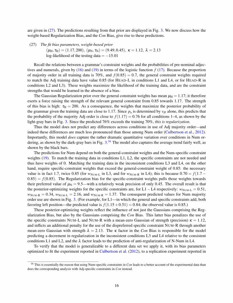
are given in (27). The predictions resulting from that prior are displayed in Fig. 3. We now discuss how theweight-based Regularization Bias, and the Con Bias, give rise to these predictions.

(27) The fit bias parameters, weight-based prior(µH,τH) = (1.17,200), (µN,τN) = (9.49,0.45), κ = 1.12, λ = 2.13log-likelihood of the testing data =−15.01

Recall the relations between a grammar’s constraint weights and the probabilities of pre-nominal adjec-tives and numerals, given by (16) and (19) in terms of the logistic function f (17). Because the proportionof majority order in all training data is 70%, and f (0.85) = 0.7, the general constraint weights requiredto match the Adj training data have value 0.85 (for HEAD-L in conditions L1 and L4, or for HEAD-R inconditions L2 and L3). These weights maximize the likelihood of the training data, and are the constraintstrengths that would be learned in the absence of a bias.

The Gaussian Regularization prior over the general constraint weights has mean µH = 1.17; it thereforeexerts a force raising the strength of the relevant general constraint from 0.85 towards 1.17. The strengthof this bias is high: τH = 200. As a consequence, the weights that maximize the posterior probability ofthe grammar given the training data are close to 1.17. Since pa is determined by vH alone, this predicts thatthe probability of the majority Adj order is close to f (1.17) = 0.76 for all conditions 1–4, as shown by thelight-gray bars in Fig. 3. Since the predicted 76% exceeds the training 70%, this is regularization.

Thus the model does not predict any differences across conditions in use of Adj majority order—andindeed these differences are much less pronounced than those among Num order (Culbertson et al., 2012).Importantly, this model does capture the rather dramatic quantitative variation over conditions in Num or-dering, as shown by the dark-gray bars in Fig. 3.16 The model also captures the average trend fairly well, asshown by the black bars.

The predictions for Num depend on both the general-constraint weights and the Num-specific constraintweights (19). To match the training data in conditions L1, L2, the specific constraints are not needed andthus have weights of 0. Matching the training data in the inconsistent conditions L3 and L4, on the otherhand, require specific-constraint weights that exceed the general-constraint weight of 0.85: the necessaryvalue is in fact 1.7, twice 0.85 (for wNUM-L in L3, and for wNUM-R in L4); this is because 0.70 = f (1.7−0.85) = f (0.85). The Regularization bias for the specific-constraint weights pulls those weights towardstheir preferred value of µN = 9.5—with a relatively weak precision of only 0.45. The overall result is thatthe posterior-optimizing weights for the specific constraints are, for L1 – L4 respectively: wNUM-L = 0.51,wNUM-R = 0.34, wNUM-L = 2.16, and wNUM-R = 1.37. The consequent predicted values for Num majorityorder use are shown in Fig. 3. (For example, for L1—in which the general and specific constraints add, bothfavoring left position—the predicted value is f (1.15+0.51) = 0.84; the observed value is 0.85.)

These posterior-optimizing weights reflect the influence of not just the Gaussians comprising the Reg-ularization Bias, but also by the Gaussians comprising the Con Bias. This latter bias penalizes the use ofthe specific constraints NUM-L and NUM-R with a mean-zero Gaussian of strength (precision) κ = 1.12,and inflicts an additional penalty for the use of the dispreferred specific constraint NUM-R through anothermean-zero Gaussian with strength λ = 2.13. The κ factor in the Con Bias is responsible for the modelpredicting a decrement in regularization in the inconsistent conditions L3 and L4 relative to the consistentconditions L1 and L2, and the λ factor leads to the prediction of anti-regularization of N-Num in L4.

To verify that the model is generalizable to a different data set we apply it, with its bias parametersoptimized to fit the experiment reported in Culbertson et al. (2012), to a replication experiment reported in

16 This is essentially the reason that using Num-specific constraints in Con leads to a better account of the experimental data thandoes the corresponding analysis with Adj-specific constraints in Con instead.

16

1 2 3 4

Condition

Pro

babi

lity

of M

ajor

ity O

rder

0.5

0.6

0.7

0.8

0.9

1.0

(µH,τH) =(1.17,200)

(µN,τN) =(9.49,0.45)

κ = 1.12λ = 2.13

AdjNumMean

Figure 3: Predictions from the weight-based prior, with fit parameter values. Plotted are the predicted probabilities of the majorityorders for {Adj, N} (green bars), {Num, N} (blue bars), and their average (red bars), superimposed on the corresponding observedvalues in the experimental data.

Culbertson (2010). The log-likelihood of the testing data in the replication experiment is −15.85, only amodest decline from −15.01, the result of the optimized fit to the original data.

While research on algorithmic-level issues of Bayesian cognitive models—e.g., appropriate resource-limited approximate optimization principles—is growing, the landscape is currently rather unclear. Theresults presented above arise from the following assumption: the learner’s search for an optimal grammar isrestricted: it is a single search starting from the neutral grammar defined by all zero constraint weights—thegrammar which assigns equal probability to all expressions. Given this constraint, multiple optimizationalgorithms prove to find the same results: those reported above. However, this restricted search proceduresometimes finds a local, not a global, optimum: the computationally expensive method of restarting thesearch from multiple hypothesized initial grammars would be needed to find the global optimum.17

5.2. Probability-based regularization priorIn section 3.2.2, we presented an alternative formalization of regularization stated directly in terms of

the probabilities of expressions, positing a prior that favors probabilities near 0 or 1. The same Con Bias isused as in the weight-based model.

The values of the prior parameters found from the optimization (26) are given in (28).18 The resultingpredicted word order probabilities are shown in Figure 4.

(28) The fit bias parameters, probability-based prior

17No set of bias parameters were found that would provide a satisfactory fit to the experimental data under the assumption thatlearners manage to compute the globally-optimal grammar; but given the severe instability of the global optimum under changes inthe bias (note 19) this may simply reflect the extremely erratic surface over which the analyst’s search for a satisfactory bias playsout.

18All optimizations were performed with the R function optim using method L-BFGS-B, with lower bounds of 0 and upperbounds of 5 for the constraint weights and (20, 20, 50) for the bias parameters (κ,λ ,γ).

17

κ = 0.41,λ = 1.04;γ = 7.35log-likelihood of the testing data =−15.52

1 2 3 4

Condition

Pro

babi

lity

of M

ajor

ity O

rder

0.5

0.6

0.7

0.8

0.9

1.0

κ = 0.41λ = 1.04γ = 7.35

AdjNumMean

Figure 4: Predictions from the probability-based prior, with fit parameters. Predicted probabilities are shown superimposed on thecorresponding observed values.

The model perfectly captures the trend in the averages (black bars), again with the Con Prior responsiblefor lowering the regularization in L3 (through κ) and lowering it still further in L4 (through λ ). The modelis not however able to capture any of the differences between Adj and Num regularization because theconstraint weights are all subject to the same pressures from the prior, as well as from the training data,which is always 30% variation in both Adj and Num. Quantitatively, the fit is only somewhat worse than forthe weight-based model, however: the log-likelihoods of the testing data are -15.52 and -15.00. Further, thismodel is preferable to the weight-based model on complexity grounds since it provides this fit with only 3bias parameters (compared to 6).

We can again apply this model with its optimized bias parameters to the replication experiment reportedin Culbertson (2010). In this case, the log-likelihood of the testing data in the replication experiment is−15.35, actually a slight improvement over −15.52, the result of the optimized fit to the original data.This is due to the fact that differences among conditions are reproduced in the replication experiment butdifferences among modifier-types less pronounced.

6. Discusssion and conclusions

6.1. Assessing the modelsThe design of the bias presented here was guided by the following desiderata:

(29) Desiderata for the learning biasa. Formal. The bias should be formally natural; e.g., the constraint weights (or expression prob-

abilities) are assessed independently—the prior is factorizable into a product of factors, eachassessing a single weight (or probability).

18

b. Computational. Search for appropriate weights given training data should not be problematic.c. Empirical. The bias should enable a good fit to the experimental data.

We have encountered several challenges to meeting these desiderata:

(30) Challenges to desiderataa. Formal: Weight combination. The probability of an expression is, in general, dependent on

multiple weights (those of the constraints it violates). [E.g., (19).]b. Computational: Disjunctive search. Weights are subject to disjunctive criteria, which can make

search for appropriate weights difficult.c. Empirical. The experimental data present a challengingly complex pattern.

The Con Bias meets the desiderata satisfactorily. A mean-zero Gaussian over prior weights is a naturalexpression of a bias for small constraint weights, and it has been used successfully in many Maxent models,which have the same formal structure as our Probabilistic Harmonic Grammar. The Con Bias factors intoa product of priors each targeting a single weight. The precision of the Gaussian assessing the weight ofan individual constraint has a clear linguistic interpretation as the strength of the bias against grammarsthat activate that constraint (by assigning it a relatively high weight). The mean-zero Gaussians present nosearch problems, and contribute exactly as theoretically expected to capturing the central average tendencyin the learning data: decreasing regularization as we go from the languages L1 and L2 with consistenthead directionality show the greatest regularization, to the inconsistent L3, and finally to the Universal-18-violating L4.

While modulated by the Con Bias, regularization is driven by the Regularization Bias, which posesthe greater challenge to formalization. Consider first the weight-based approach to this bias (section 5.1).At the formal level, this prior achieves factorizability: it is the product of two factors, each independentlyevaluating a single weight, penalizing deviation from a constraint-specific preferred value. However, thisprior does not necessarily, even in principle, actually achieve the goal of disfavoring probabilities near 0.5,because probabilities are often determined by differences of weights, and a difference may be small evenif the individual weights are not. This is the challenge that weight combination presents to an approach toregularization based directly on weights (30a).

In the probability-based approach to the Regularization Bias (section 5.2), the formal status of the prioris largely satisfactory. It is a product of factors each assessing an individual probability, each factor being ascaled beta distribution. The beta distribution is the conjugate prior for our likelihood function, a binomial;it is formally natural in this sense. By construction, this prior favors probabilities close to 0 or 1, providinga regularization force that is not compromised by the problem of weight combination which plagues theweight-based prior.

An important difference between the two forms of the Regularization Bias is the extent to which reg-ularization is formalized as occurring within the grammatical system or outside it, in the following sense.A function of a grammatical analysis is to recast the surface forms of expressions into a more fundamentaldescription; in the PHG case, an expression is analyzed as a set of weighted constraint violations. If this isthe correct way to analyze regularization, it should be enlightening to state this bias in terms of constraintweights. This is rejected by the probability-based formalization of the Regularization Bias, which deals withthe surface properties of expressions, in particular, their frequencies. To the extent that this formalizationof the Regularization Bias is to be preferred, we can conclude that regularization is farther removed fromthe grammar proper, consistent with the cognition-general status of regularization. However a bias againstinconsistency may also be cognition-general, and we have seen that the consistency bias in word order canbe naturally expressed within a constraint-based grammar: this may be seen as the reflex, within grammar,

19

of a wider-scope principle of cognition. Whether regularization has the same status is a question addressedby these two formalizations of the prior.

Turning to the computational desideratum, we observed difficulties with the weight-based prior. Thelearner’s search for appropriate weights given their training data faces a challenge arising from the inher-ently disjunctive search space (30b): either wHEAD-L or wHEAD-R is zero, and similarly for wNUM-L,wNUM-R,creating a search space with 4 distinct regions. Finding a globally optimal set of weights would essentiallyrequire running 4 separate searches, starting in each one of these regions. This is related to the problem ofweight combination, since it arises because it is only [wHEAD-L−wHEAD-R]—and not wHEAD-L or wHEAD-Rindividually—that matters. For the Regularization Bias to disfavor probabilities near 0.5, it must disfavorgrammars in which [wHEAD-L−wHEAD-R] is near 0, which cannot be done via independent penalties on in-dividual weights—unless we take the step of reducing the weight values so that the smaller is always 0,thereby creating the disjunction problem.19

The probability-based Regularization Bias does not appear to suffer from these search problems, andthus is to be favored from the perspective of computational tractability.

With respect to the empirical desideratum, both models present fairly successful fits to the data, cap-turing the main patterns of interest. The clearest difference along this dimension is in the two models’differentiation of adjectives and numerals. The weight-based prior model predicts (in fact slightly exagger-ates) the asymmetry present in the data, while the probability-based prior model fails to predict any suchasymmetry (for reasons discussed in section 5.2). However, in sum, the results favor the probability-basedprior: while faring somewhat less well on the empirical desideratum, it is less complex and does not suf-fer the computational problems observed in the weight-based model of the learner’s search for an optimalgrammar given the training data.

6.2. Returning to the typology

We have seen that both models capture the main behavioral asymmetries in the artificial language learn-ing experiment—both models predict greater regularization for consistent ordering patterns (L1, L2) com-pared to inconsistent patterns (L3, L4), and substantially less use of the majority input order (in fact under-regularization) for the pattern originally ruled out by Greenberg’s Universal 18 (L4). Insofar as the behav-ioral results mirror the typology in Table 1, the models thus also capture, qualitatively, the cross-linguisticdistribution of these ordering patterns. The Regularization Bias, exhibited by learners in the experiment,and captured by the modeling results, is also apparent in the typology; in the WALS sample, there are 966languages determined to have a clearly preferred ordering pattern, but only 117 languages (not shown inTable 1) with no clear preference for either Adj or Num or both. This suggest that linguistic variation isstrongly curbed by such a regularizing force.

Nevertheless, the experimental results and the models we have tested here do not capture every asymme-try in Table 1. In particular there is no prediction that L2 should differ from L1 despite the clear differencetypologically; both are consistent patterns, and no distinction is made here between the constraints HEAD-Rand HEAD-L. In this case, the discrepancy between our modeling results and the typology are likely due tothe choice of English learners as experimental participants. If English learners have a preference for theirnative language pattern, L1, then any preference they might have shown for L2 could be masked by this (seeCulbertson et al., 2012, for additional discussion).20

19 A further practical difficulty arises because the globally optimal weights are also quite unstable as the bias is varied: the optimalweights instantaneously jump as the bias crosses some critical point at which the global optimum shifts from one disjunctive weightcombination to another. This makes quite difficult the analyst’s search for a set of prior-parameters which would yield satisfactoryresults under global weight optimization.

20How the bias displayed by artificial-language learners might both reflect native-like priors and effects of previously learnedlanguages might be explainable through an assumed hierarchical structure in the Bayesian model—perhaps along the following

20

6.3. Conclusion

The biases of learners have long been of interest to linguists and psychologists exploring the powerand limitations of the human language learning faculty. One source of evidence for such biases comesfrom linguistic typology—a potential reflection of learners’ preferences. We have proposed here a solutionto an ongoing challenge in understanding this evidence, namely how to formulate a theory which bothaccommodates typologically rare languages while at the same time explains their rarity. Within a constraint-based approach, closely related to Optimality Theory—Probabilistic Harmonic Grammar—we explain therelative rarity of a given language type by hypothesizing soft biases which target the constraints needed toderive it. We formalize these soft biases in terms of a Bayesian prior on learning. This solution providesnot only a means for qualitatively understanding typology, but also a tool for understanding the behavioralresults of language learning experiments. Modeling these results allows us to determine, quantitatively, theprior bias against particular constraints, and how this prior influences what grammars learners acquire.

The major contribution of our solution is a new formalization of the role of Con—the set of constraintsused to derive language types in our PHG theory. In standard Optimality Theory, the predictive power ofthe theory of typology comes from the particular set of constraints that the theorist posits are included inCon. Language types are either possible or impossible with respect to Con. In the theory proposed here, theset of constraints is more inclusive, and the predictive power comes from the cost associated with particularconstraints. Some constraints might be so costly that grammars in which they are active are very unlikelyto be acquired, and thus the linguistic patterns which would be optimal according to these grammars areeffectively impossible. However, languages types which are possible but rare are included in the typology,and their rarity is explained as a result of the cost of activating the constraints needed to derive them.

That the theory we have developed here to analyze learning biases and their relation to typology is for-malized within PHG is, we believe, an important asset. First, PHG makes clear contact with a tradition oftypological analysis in Optimality Theory—researchers interested in modeling language learning data canmake use of the types of constraints already motivated within OT. Second, PHG is a linguistic implementa-tion of Maxent models, and as such, tools developed within the machine learning community can be used toalter or augment what we have proposed here as needed.

The modeling results we have presented illustrate that our PHG theory is able to capture interestingfeatures of the artificial language learning experiment reported in Culbertson et al. (2012). The experimentwas designed to test the interaction between (i) learning biases related to the typological asymmetry knownas Universal 18, and (ii) a cognitive bias, regularization, which disfavors variation. We showed that, sub-ject to certain starting conditions, a model which encodes the regularization bias in terms of weights ofconstraints in a grammar (dispreferring values near zero) reveals that learners have a clear bias in favor ofconsistent-head-ordering languages (derived from a set of general head-alignment constraints) and againstinconsistent languages, especially against the particular pattern Adj-N, N-Num. This is as predicted basedon the typology. However, encoding regularization in this way comes at a computational cost, making thegrammar space quite complex to search and therefore making the inference problem more difficult—clearlyat odds with the guiding idea that learning biases serve to aid language acquisition.

Encoding regularization in terms of the probabilities derived from grammars (following Reali & Grif-fiths, 2009; Culbertson & Smolensky, 2012) solves this computational problem while still providing a goodempirical fit to the major trends in the experimental data, revealing a clear quantitative cost of the con-

lines. A learner may acquire multiple languages over a lifetime, possibly including an artificial language learned in a laboratoryexperiment. Each distinct language has its own learned grammar, and in each case the grammar learning is governed by the type ofprior we discuss in this paper. That prior, specified by a set of parameters, is in turn governed by a hyperprior over those parameters.The grammar-learning prior shifts as the languages it accounts for are acquired: learning English will adjust the prior expectationabout word orders in languages generally. If the hyperprior is quite strong, however, as new languages are acquired, the prior willonly shift slightly away from its initial state.

21

straints that are hypothesized, based on typological patterns, to be disfavored in our Bayesian prior. In thisapproach, the force of regularization is in some sense more external to the grammar, as it doesn’t directlytarget constraint weights, but the probabilities that result from them. This is potentially a desirable resultsince a body of evidence suggest that the regularization bias is cognition-general rather than specific to thelanguage faculty.

References

Anttila, A. (1997). Deriving variation from grammar. In F. Hinskens, R. van Hout, & L. Wetzels (Eds.),Variation, change and phonological theory (pp. 35–68). Philadelphia: John Benjamins.

Baker, M. (2001). The atoms of language: The mind’s hidden rules of grammar. New York, NY: BasicBooks.

Biberauer, T., Holmberg, A., & Roberts, I. (to appear). A syntactic universal and its consequences. LinguisticInquiry.

Bickel, B. (2007). Typology in the 21st century: Major current developments. Linguistic Typology, 11,239–251.

Bod, R., Hay, J., & Jannedy, S. (Eds.) (2003). Probabilistic Linguistics. Cambridge, MA: MIT Press.

Boersma, P. (1998). Functional phonology: Formalizing the interactions between articulatory and percep-tual drives. Holland Academic Graphics/IFOTT.

Chater, N., & Manning, C. D. (2006). Probabilistic models of language processing and acquisition. Trendsin Cognitive Sciences, 10, 335 – 344.

Chen, S., & Rosenfeld, R. (2000). A survey of smoothing techniques for ME models. Speech and AudioProcessing, IEEE Transactions on, 8, 37–50.

Chomsky, N. (1965). Aspects of the Theory of Syntax. Cambridge, MA: MIT Press.

Chomsky, N. (1980). On binding. Linguistic Inquiry, 11, 1–46.

Chomsky, N. (1981a). Lectures on Government and Binding. Dordrecht: Foris.

Chomsky, N. (1981b). Markedness and core grammar. In A. Belletti, L. Brandi, & L. Rizzi (Eds.), Theoryof markedness in core grammar (pp. 123–146). Pisa: Scuola Normale Superiore di Pisa.

Chomsky, N. (1986). Barriers. Cambridge, MA: MIT Press.

Chomsky, N. (1998). Minimalist inquiries: The framework. Number 15 in MIT Working Papers in Linguis-tics. Cambridge, MA: MIT, Dept. of Linguistics.

Cinque, G. (1994). On the evidence for partial n-movement in the Romance DP. In G. Cinque, J. Koster,J.-Y. Pollock, L. Rizzi, & R. Zanuttini (Eds.), Paths towards Universal Grammar: Studies in Honor ofRichard S. Kayne (pp. 85–110). Georgetown: Georgetown University Press.

Cinque, G. (2005). Deriving Greenberg’s Universal 20 and its exceptions. Linguistic Inquiry, 36, 315–332.

Culbertson, J. (2010). Learning biases, regularization, and the emergence of typological universals insyntax. Ph.D. thesis Johns Hopkins University Baltimore, MD.

22

Culbertson, J. (2012). Typological universals as reflections of biased learning: Evidence from artificiallanguage learning. Language and Linguistics Compass, 6, 310–329.

Culbertson, J., & Smolensky, P. (2012). A Bayesian model of biases in artificial language learning: Thecase of a word-order universal. Cognitive Science, (pp. 1–31).

Culbertson, J., Smolensky, P., & Legendre, G. (2012). Learning biases predict a word order universal.Cognition, 122, 306–329.

Curtin, S., & Zuraw, K. (2002). Explaining constraint demotion in a developing system. In Proceedings ofthe Boston University conference on language development (pp. 118–129). Citeseer volume 26.

Dryer, M. (2008a). Order of adjective and noun. In M. Haspelmath, M. S. Dryer, D. Gil, & B. Comrie(Eds.), The World Atlas of Language Structures Online chapter 87. Munich: Max Planck Digital Library.

Dryer, M. (2008b). Order of numeral and noun. In M. Haspelmath, M. S. Dryer, D. Gil, & B. Comrie (Eds.),The World Atlas of Language Structures Online chapter 89. Munich: Max Planck Digital Library.

Dryer, M. (2012). Are word order correlations lineage-specific? Talk given at the 86th Annual Meeting ofthe Linguistic Society of America.

Dunn, M., Greenhill, S., Levinson, S., & Gray, R. (2011). Evolved structure of language shows lineage-specific trends in word-order universals. Nature, 473, 79–82.

Evans, N., & Levinson, S. C. (2009). The myth of language universals: Language diversity and its impor-tance for cognitive science. Behavioral and Brain Sciences, 32, 429–448.

Finkel, J. R., & Manning, C. D. (2009). Hierarchical bayesian domain adaptation. In Proceedings of HumanLanguage Technologies: The 2009 Annual Conference of the North American Chapter of the Associa-tion for Computational Linguistics NAACL ’09 (pp. 602–610). Stroudsburg, PA, USA: Association forComputational Linguistics.

Finley, S., & Badecker, W. (2008). Substantive biases for vowel harmony languages. In J. Bishop (Ed.),Proceedings of WCCFL 27 (pp. 168–176).

Gold, E. M. (1967). Language identification in the limit. Information Control, 10, 447–474.

Goldwater, S., & Johnson, M. (2003). Learning OT constraint rankings using a maximum entropy model. InProceedings of the Workshop on Variation within Optimality Theory (pp. 111–120). Stockholm: Stock-holm University.

Greenberg, J. (1963). Some universals of grammar with particular reference to the order of meaningfulelements. In J. Greenberg (Ed.), Universals of Language (pp. 73–113). Cambridge, MA: MIT Press.

Grimshaw, J. (1997). Projection, heads, and optimality. Linguistic Inquiry, 28, 373–422.

Hayes, B., Siptar, P., Zuraw, K., & Londe, Z. (2009). Natural and unnatural constraints in hungarian vowelharmony. Language, 85.

Hayes, B., & Wilson, C. (2008). A maximum entropy model of phonotactics and phonotactic learning.Linguistic Inquiry, 39, 379–440.

Hudson Kam, C., & Newport, E. (2009). Getting it right by getting it wrong: When learners changelanguages. Cognitive Psychology, 59, 30–66.

23

Jarosz, G. (2010). Implicational markedness and frequency in constraint-based computational models ofphonological learning. Journal of Child Language, 37, 565–606.

Jesney, K., & Tessier, A. (2011). Biases in harmonic grammar: the road to restrictive learning. NaturalLanguage & Linguistic Theory, 29, 251–290.

Kayne, R. (1994). The Antisymmetry of Syntax. Cambridge, MA: MIT Press.

Laenzlinger, C. (2005). French adjective ordering: perspectives on dp-internal movement types. Lingua,115, 645–689.

Legendre, G., Miyata, Y., & Smolensky, P. (1990). Harmonic grammar — a formal multi level connectionisttheory of linguistic well formedness: Theoretical foundations. In Proceedings of the Twelfth AnnualConference of the Cognitive Science Society (pp. 388–395). Cambridge, MA.

Legendre, G., Raymond, W., & Smolensky, P. (1993). An optimality-theoretic typology of case and gram-matical voice systems. In Proceedings of the Nineteenth Annual Meeting of the Berkeley LinguisticsSociety (pp. 464–478). University of California, Berkeley: Berkeley Linguistics Society volume 464.

McCarthy, J. (2002). A thematic guide to Optimality Theory. New York: Cambridge University Press.

McCarthy, J., & Prince, A. (1994). The emergence of the unmarked: Optimality in prosodic morphology.In M. Gonzàlez (Ed.), NELS 24 (pp. 333–379). University of Massachussetts Amherst: GLSA volume 2.

Mitchell, T. (1980). The need for biases in learning generalizations. Technical Report CBM-TR-5-110 Department of Computer Science, Laboratory for Computer Science Research, Rutgers Univ. NewBrunswick, NJ.

Moreton, E. (2008). Analytic bias and phonological typology. Phonology, 25, 83–127.

Moreton, E., & Pater, J. (to appear). Structure and substance in artificial-phonology learning. Language andLinguistics Compass, .

Nagy, N., & Heap, D. (1998). Francoprovençal null subjects and constraint interaction. In CLS 34: ThePanels (pp. 151–166). Chicago: The Chicago Linguistic Society.

Newmeyer, F. J. (2010). Accounting for rare typological features in formal syntax: three strategies and somegeneral remarks. In Rethinking universals: how rarities affect linguistic theory (pp. 195–222). New York:Mouton de Gruyter.

Pater, J. (2009). Weighted constraints in generative linguistics. Cognitive Science, 33, 999–1035.

Pater, J. (2011). Emergent systemic simplicity (and complexity). McGill Working Papers in Linguistics, .

Philip, J. (to appear). (dis)harmony, the head-proximate filter, and linkers. Journal of Linguistics, .

Plank, F., & Filimonova, E. (2000). The universals archive. Sprachtypologie und Universalienforschung,53, 109–123.

Prince, A., & Smolensky, P. (1993/2004). Optimality Theory: Constraint interaction in generative grammar.New York, NY. Technical Report, Rutgers University and University of Colorado at Boulder, 1993.Rutgers Optimality Archive 537, 2002. Revised version published by Blackwell 2004.

Prince, A., & Tesar, B. (2004). Learning phonotactic distributions. In R. Kager, J. Pater, & W. Zonneveld(Eds.), Constraints in phonological acquisition (pp. 245–291). Cambridge University Press.

24

Pullum, G., & Scholz, B. C. (2002). Empirical assessment of stimulus poverty arguments. The LinguisticReview, 19, 9–50.

Pycha, A., Nowak, P., Shin, E., & Shosted, R. (2003). Phonological rule-learning and its implications for atheory of vowel harmony. In Proceedings of the 22nd West Coast Conference on Formal Linguistics (pp.101–114). Somerville, MA: Cascadilla Press volume 22.

R Development Core Team (2010). R: A language and environment for statistical computing. R Foundationfor Statistical Computing Vienna.

Reali, F., & Griffiths, T. L. (2009). The evolution of frequency distributions: Relating regularization toinductive biases through iterated learning. Cognition, 111, 317 – 328.

Samek-Lodovici, V. (2005). Prosody-syntax interaction in the expression of focus. Natural Language andLinguistic Theory, 23, 687–755.

Sells, P. (2001). Structure, Alignment, and Optimality in Swedish. Stanford, CA: CSLA Publications.

Smith, D., & Eisner, J. (2007). Bootstrapping feature-rich dependency parsers with entropic priors. InProceedings of the 2007 Joint Conference on Empirical Methods in Natural Language Processing andComputational Natural Language Learning (EMNLP-CoNLL) (pp. 667–677).

Smolensky, P. (1996). The initial state and ‘richness of the base’in optimality theory. Rutgers OptimalityArchive, 293.

St. Clair, M. C., Monaghan, P., & Ramscar, M. (2009). Relationships between language structure andlanguage learning: The suffixing preference and grammatical categorization. Cognitive Science, 33,1317–1329.

Steddy, S., & Samek-Lodovici, V. (2011). On the ungrammaticality of remnant movement in the derivationof Greenberg’s Universal 20. Linguistic Inquiry, 42, 445–469.

Travis, L. (1984). Parameters and Effects of Word Order Variation. Ph.D. dissertation MIT.

Travis, L. (1989). Parameters of phrase structure. In M. R. Baltin, & A. S. Kroch (Eds.), Alternativeconceptions of phrase structure (pp. 263–279). Chicago: University of Chicago Press.

Vogel, R. (2002). Free relative constructions in ot syntax. In G. Fanselow, & C. Féry (Eds.), Resolving Con-flicts in Grammars: Optimality Theory in Syntax, Morphology, and Phonology (pp. 119–162). Hamburg:Helmut Buske Verlag.

Weir, M. W. (1972). Probability performance: Reinforcement procedure and number of alternatives. TheAmerican Journal of Psychology, 85, 261–270.

Wilson, C. (2006). An experimental and computational study of velar palatalization. Cognitive Science, 30,945–982.

25