cohabitation, marriage, relationship stability and child ... · rory gallagher, kathleen kiernan,...
TRANSCRIPT
Cohabitation, marriage, relationship stability and child outcomes: an update
IFS Commentary C120 Claire Crawford Alissa Goodman Ellen Greaves Robert Joyce
Cohabitation, marriage, relationship stability and child outcomes: an update
Claire Crawford
Alissa Goodman
Ellen Greaves
Robert Joyce
Institute for Fiscal Studies
Copy-edited by Judith Payne
The Institute for Fiscal Studies 7 Ridgmount Street London WC1E 7AE

Published by
The Institute for Fiscal Studies 7 Ridgmount Street London WC1E 7AE
Tel: +44 (0)20 7291 4800 Fax: +44 (0)20 7323 4780 Email: [email protected]
Website: http://www.ifs.org.uk
© The Institute for Fiscal Studies, July 2011
ISBN: 978-1-903274-85-9

Preface
The authors are very grateful to the Nuffield Foundation for supporting this work as part of a wider project, ‘Births out of Wedlock and Cognitive and Social Development throughout Childhood: A Quantitative Analysis’ (grant number CPF/37467).
The authors would also like to extend particular thanks to Dan Anderberg, John Ermisch, Hayley Fisher, Rory Gallagher, Kathleen Kiernan, Penny Mansfield, Jo Miles, Debora Price, Rebecca Probert, Kitty Stewart and Sharon Witherspoon for helpful comments and advice.
All views expressed are those of the authors.
Contents
Executive summary 1
1.
Introduction 6
2. Data and methodology 9 2.1 The data sets that we use 9 2.2 Measuring child development 10 2.3 Measuring relationship status 12 2.4 Our samples 13 2.5 Features of an ideal data set
13
3. Evidence from the Millennium Cohort Study 15 3.1 Outcomes of children born to married and cohabiting couples 15 3.2 Characteristics of married and cohabiting couples 17 3.3 Regression results 18 3.4 Summary
22
4. Evidence from the British Cohort Study 23 4.1 Outcomes of children born to married and cohabiting couples 23 4.2 Characteristics of married and cohabiting couples 24 4.3 Regression results 26 4.4 Summary
28
5. Marital status, relationship stability and child outcomes 29 5.1 Measuring relationship stability 29 5.2 Does marriage improve relationship stability? 30 5.3 Does relationship instability drive the correlation between cohabitation
and child outcomes? 33
5.4 Summary
36
6.
Conclusions 37
Appendix A. Additional MCS analysis 38 Appendix B. Additional BCS analysis 45 Appendix C. MCS–BCS comparison 53 Appendix D. Relationship stability
54
References 57

1
© Institute for Fiscal Studies, 2011
Executive summary
Introduction
• It is well known that children born to married parents achieve better cognitive and social outcomes, on average, than children born into other family forms, including cohabiting unions. The existence of such gaps is potentially important, given the long-term consequences of childhood cognitive and socio-emotional development for education, labour market and other outcomes in adulthood.
• It is widely recognised that marital status may not be the cause of these differences, however. Cohabiting couples may differ from married couples in many ways other than their formal marital status, such as their education or the love and commitment in their relationship. Differences in outcomes between children whose parents are married and those who cohabit may simply reflect these differences in other characteristics rather than be caused by marriage.
• Goodman and Greaves, in Cohabitation, Marriage and Child Outcomes (IFS Commentary 114, 2010a), provided recent, systematic evidence on these issues for a sample of children born in the UK in the early 2000s (the Millennium Cohort Study, MCS) and considered outcomes up to age 5. This Commentary builds on their work in two important ways. First, it extends their analysis using the MCS to outcomes for children at age 7, in order to investigate the extent to which the magnitude and drivers of the gaps in outcomes between children born and raised in different family forms evolve as children age. Second, it makes use of data from the children of the British Cohort Study (BCS). The BCS is a longitudinal survey that contains very detailed background information about a cohort of individuals born in 1970, providing us with information about these people throughout their lives, starting long before they made their marriage decisions and including them becoming parents. The availability of such information ensures that we are better able to account for the selection of parents into marriage, without controlling away any of the potential effects of marriage on child outcomes. In doing so, we aim to inform the ongoing policy debate about the merits of encouraging individuals to enter marriage before they bear children.
Data and methodology
• Our study is based on data from the Millennium Cohort Study and the British Cohort Study. The MCS is a longitudinal study of children which initially sampled almost 19,000 new births across the UK in the early 2000s, with follow-ups at 9 months, 3 years, 5 years and 7 years. The BCS is a longitudinal study of all individuals born in Great Britain in a particular week in April 1970, which has surveyed them at various points throughout their lives, the latest at age 38 in 2008. Crucially for our purposes, in the age 34 wave (in 2004), the children of half of the cohort members were randomly selected to take cognitive tests, and parents answered an additional battery of questions about those children. The children of the BCS cohort members (rather than the cohort members themselves) are therefore the children of interest in this Commentary.
• In both the MCS and the BCS, children’s cognitive development is measured using the British Ability Scales (BAS) and children’s socio-emotional development is derived from parental responses to the Strengths and Difficulties Questionnaire (SDQ). We construct average, age-adjusted scores for each child, which we use as our measures of cognitive and socio-emotional development.
Cohabitation, marriage, relationship stability and child outcomes: an update
2
© Institute for Fiscal Studies, 2011
• To carry out our analysis, we adopt a simple ordinary least squares (OLS) regression approach. We start by regressing child development on parents’ marital status to estimate the ‘raw’ relationship between the two. We then sequentially add controls for other ways in which married and cohabiting parents differ – starting with those that are most likely to reflect selection into marriage (for example, ethnicity) and moving progressively towards those that might be regarded as reflecting both selection and a possible pathway through which marriage might have a causal effect (for example, relationship quality) – to see what the addition of these characteristics does to the ‘impact’ of marriage on child development.
Evidence on the relationship between marital status and child development
Results from our MCS analysis
• Children born to cohabiting parents exhibit a small deficit (of around 10–20% of a standard deviation) in cognitive development at ages 3, 5 and 7 compared with children born to married parents, but this deficit is largely accounted for by the fact that cohabiting parents have lower educational qualifications than married parents. While it is possible that the decision to be married might lead some parents to attain higher educational qualifications, this effect is likely to be small. Our judgement is that the gap in cognitive development between children born to cohabiting parents and those born to married parents is largely accounted for by their parents’ lower level of education, and is not a consequence of parental marital status.
• Children born to cohabiting parents exhibit a larger deficit (of around 30% of a standard deviation) in socio-emotional development (relative to cognitive development) at ages 3, 5 and 7 compared with children born to married parents. This gap is reduced by more than half, but remains statistically significant, once differences in parental education and socio-economic status are controlled for. This suggests that the majority of the gap in socio-emotional development between children born to cohabiting parents and those born to married parents is accounted for by their parents’ lower level of education and income. Once differences in family structure, including the likelihood of a pregnancy being unplanned and relationship quality when the child is 9 months old, are also controlled for, the gap in socio-emotional development between the children of married and cohabiting parents becomes even smaller, and is statistically insignificant.
• However, because many of these factors – such as education, socio-economic status and relationship quality – are observed after marriage decisions have been taken, this analysis using the MCS is not able to perfectly distinguish the extent to which such differences reflect the sort of people who choose to marry in the first place from how much they are a positive product of marriage itself.
Results from our BCS analysis
• Our analysis using the BCS data is able to overcome this issue, as the data set provides us with very rich information about one of the child’s parents observed during his or her own childhood, long before marriage decisions were taken. For example, we have information on parental cognitive and socio-emotional development measured when they were children. By including such characteristics in our models, we can be sure that we are capturing selection effects rather than ‘controlling away’ any effects of marital status on child development.
Executive summary
3
© Institute for Fiscal Studies, 2011
• However, while the BCS provides us with a wealth of additional information that is extremely valuable to our study, it must be acknowledged that it is far from a representative sample of children. This is driven by a number of factors, including that almost half of the original sample had left the BCS by age 34 (when the random sample of cohort members’ children was taken), that the children in our sample must have at least one parent aged between 18 and 31 at the time of the child’s birth, and that children who did not live with the BCS cohort member in 2004 cannot appear in our sample. It is worth noting, however, that our conclusions remain unchanged if we focus on the children of female cohort members only (whom we expect to be less affected by these sample restrictions).
• Notwithstanding these caveats, however, the analysis we conduct using the BCS strengthens the conclusions drawn from our MCS results: the differences in cognitive and socio-emotional development between children born to married and those born to cohabiting parents mainly or entirely reflect the selection of different types of people into marriage, rather than effects of marriage itself. That is to say, after controlling for differences between couples that are observed in the parent’s own childhood and early adulthood, before they entered the relationship into which their child was born, we find no statistically significant difference between the cognitive and socio-emotional development of children born to parents who choose to be married compared with those who cohabit.
• Amongst these factors, parental cognitive ability represents the most important source of selection in our model. We estimate that the higher average cognitive ability of married parents over cohabiting ones explains about one-fifth of the gap in cognitive development between those groups of children, and about one-seventh of the gap in socio-emotional development, even after accounting for differences in other observable characteristics.
A role for relationship stability?
• It is widely recognised that cohabiting parents are more likely to split up than married ones, and that the outcomes for children whose parents separate are particularly poor. Using a similar regression framework to that described above, we also investigate the link between marital status and the likelihood of separation, and examine the extent to which relationship breakdown amongst cohabiting couples may lead to poorer outcomes for their children. In both cases, our objective is simply to consider the extent to which differences in other observable characteristics are able to explain the relationships that other commentators have observed.
• We find that cohabiting parents are more likely to split up by the time their child turns 3 than married parents. However, this gap is almost entirely eliminated after accounting for other observable characteristics that we believe wholly or largely reflect selection. This suggests that the vast majority of the raw gap in the likelihood of separation between cohabiting and married couples is driven by the selection of different types of people into marriage, rather than by a causal effect of marriage on relationship stability.
• Moreover, while cohabiting couples are more likely to separate than married ones, this does not appear to have a detrimental effect on their children’s cognitive or socio-emotional development, once we have taken account of the other ways in which cohabiting and married couples differ. This is the case even among the subgroup of children born to cohabiting parents who subsequently split up, where the ‘raw’ outcome gaps were particularly large. As with our earlier analyses using the MCS and the BCS, this suggests that marriage does not have a causal effect on child outcomes.
Cohabitation, marriage, relationship stability and child outcomes: an update
4
© Institute for Fiscal Studies, 2011
Conclusions
• The Prime Minister, David Cameron, has repeatedly expressed his desire to support marriage through the tax system, presumably at least partly based on a belief that such family situations are better for children along a number of dimensions. However, our findings suggest that the gaps in cognitive and socio-emotional development between children born to married parents and those born to cohabiting parents mainly or entirely reflect the fact that different types of people choose to get married (the selection effect), rather than that marriage has an effect on relationship stability or child development. On the basis of this evidence, therefore, child development does not provide a convincing rationale for policies that encourage parents to get married before they bear children. It does, however, provide strong support for policymakers to continue to try to increase the educational attainment of today’s children (tomorrow’s parents) as a means of improving the outcomes of future generations of children.
Executive summary
5
© Institute for Fiscal Studies, 2011
What does this Commentary add to Goodman and Greaves (2010a)?
• This Commentary builds on the work of Goodman and Greaves in two important ways. First, it extends their analysis using the MCS to outcomes for children at age 7. Second, it makes use of data from the children of the British Cohort Study (BCS), to better account for the selection of parents into marriage, without controlling away any of the potential effects of marriage on child outcomes.
What do the age 7 MCS results add?
• Chapter 3 shows that the gap in cognitive development between children born to cohabiting and married parents in the MCS significantly increases between the ages of 3 and 7, from just under 10% of a standard deviation at age 3 to just under 20% of a standard deviation at age 7. This increase is largely driven by the improvement in test scores amongst children from ethnic minority backgrounds and those whose mother was born outside the UK, most of whom are married.
• The gap in socio-emotional development insignificantly decreases – from around 30% of a standard deviation at age 3 to 27% of a standard deviation at age 7 – over the same period.
What does the BCS analysis add?
• The main issue with the MCS analysis is that many of the factors used to control for observable differences between parents who choose to be married and those who cohabit – such as education, socio-economic status and relationship quality – are observed after marriage decisions have been taken. To the extent that marriage may affect such characteristics, therefore, this analysis risks ‘controlling away’ some of the effects of marriage on child development by including such characteristics in the model.
• Our analysis using the BCS data is able to overcome this issue, as the data set provides us with very rich information about one of the child’s parents observed during his or her own childhood, long before marriage decisions were taken. By including such characteristics in our models, we can be sure that we are capturing the selection of different types of people into marriage, but not ‘controlling away’ any effects of marital status on child development.
• The analysis we conduct using the BCS strengthens the conclusions drawn from our MCS results, that differences in cognitive and socio-emotional development between children born to married parents and those born to cohabiting parents mainly or entirely reflect the selection of different types of people into marriage, rather than any effect of marriage on child development. In fact, after controlling for differences between couples that are observed in the parent’s own childhood and early adulthood, before they entered the relationship into which their child was born, we find no statistically significant difference between the cognitive and socio-emotional development of children born to parents who choose to be married and children born to parents who cohabit.
• This lends greater weight to the conclusion reached by Goodman and Greaves, who suggested – as we do in this Commentary – that there does not seem to be a strong reason in terms of child development for policymakers to encourage parents to get married before they bear children.
6
© Institute for Fiscal Studies, 2011
1. Introduction
It is well known that children born to married parents achieve better cognitive and social outcomes, on average, than children born into other family forms, including cohabiting unions.1 The existence of such gaps is potentially important, given the long-term consequences of childhood cognitive and socio-emotional development for education, labour market and other outcomes, such as health and crime, in adulthood.2 It is widely recognised, however, that marital status may not be the cause of these differences. This Commentary seeks to provide evidence on these issues, using data on recent cohorts of children in the UK, in order to inform the ongoing policy debate.
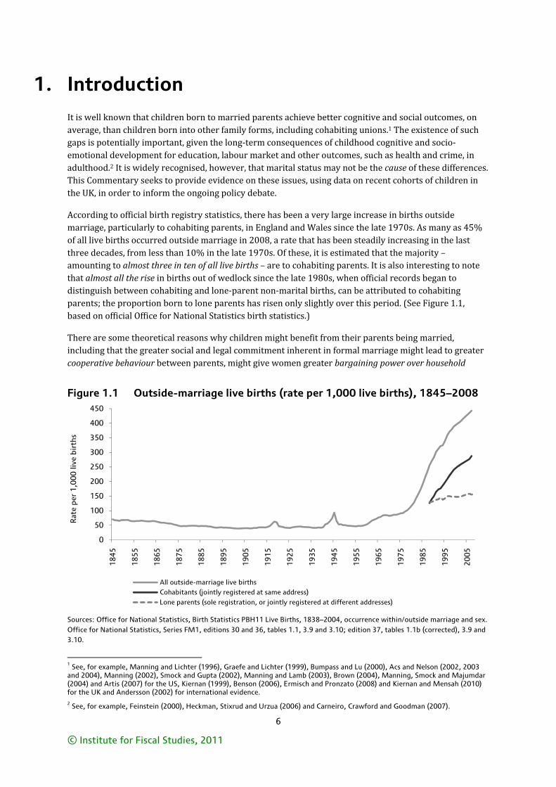
According to official birth registry statistics, there has been a very large increase in births outside marriage, particularly to cohabiting parents, in England and Wales since the late 1970s. As many as 45% of all live births occurred outside marriage in 2008, a rate that has been steadily increasing in the last three decades, from less than 10% in the late 1970s. Of these, it is estimated that the majority – amounting to almost three in ten of all live births – are to cohabiting parents. It is also interesting to note that almost all the rise in births out of wedlock since the late 1980s, when official records began to distinguish between cohabiting and lone-parent non-marital births, can be attributed to cohabiting parents; the proportion born to lone parents has risen only slightly over this period. (See Figure 1.1, based on official Office for National Statistics birth statistics.)
There are some theoretical reasons why children might benefit from their parents being married, including that the greater social and legal commitment inherent in formal marriage might lead to greater cooperative behaviour between parents, might give women greater bargaining power over household
Figure 1.1 Outside-marriage live births (rate per 1,000 live births), 1845–2008
Sources: Office for National Statistics, Birth Statistics PBH11 Live Births, 1838–2004, occurrence within/outside marriage and sex. Office for National Statistics, Series FM1, editions 30 and 36, tables 1.1, 3.9 and 3.10; edition 37, tables 1.1b (corrected), 3.9 and 3.10.
1 See, for example, Manning and Lichter (1996), Graefe and Lichter (1999), Bumpass and Lu (2000), Acs and Nelson (2002, 2003 and 2004), Manning (2002), Smock and Gupta (2002), Manning and Lamb (2003), Brown (2004), Manning, Smock and Majumdar (2004) and Artis (2007) for the US, Kiernan (1999), Benson (2006), Ermisch and Pronzato (2008) and Kiernan and Mensah (2010) for the UK and Andersson (2002) for international evidence. 2 See, for example, Feinstein (2000), Heckman, Stixrud and Urzua (2006) and Carneiro, Crawford and Goodman (2007).
0
50
100
150
200
250
300
350
400
450
1845
1855
1865
1875
1885
1895
1905
1915
1925
1935
1945
1955
1965
1975
1985
1995
2005
Rat
e pe
r 1,
000
live
birt
hs
All outside-marriage live birthsCohabitants (jointly registered at same address)Lone parents (sole registration, or jointly registered at different addresses)
Introduction
7
© Institute for Fiscal Studies, 2011
resources or might reduce parental stress – all of which could lead to better child outcomes.3 Understandably, therefore, the consequences of the growth in non-marital births for children’s well-being, and their cognitive and socio-emotional skills, have become the subject of considerable scrutiny.
Our own previous work has shown that children born to married parents score around 10% of a standard deviation higher in cognitive tests and 30% of a standard deviation higher on socio-emotional scales at age 3 than children born to cohabiting parents (Goodman and Greaves, 2010a). It is widely recognised that marital status may not be the cause of these differences, however. Cohabiting couples may differ from married couples in many ways other than their formal marital status, such as their income, ethnicity, education or the love and commitment in their relationship.4 Differences in outcomes between children whose parents are married and those who cohabit may therefore simply reflect these differences in other characteristics rather than be caused by marriage. This is sometimes referred to as the ‘selection issue’.
Empirically, researchers have struggled to find strategies that adequately deal with this selection issue. One common approach is to try to take account of observable differences between married and cohabiting parents using simple regression techniques. Goodman and Greaves (2010a) adopted this methodology to provide systematic evidence on these issues for recent cohorts of children born in the UK. They started by documenting the gaps in cognitive and socio-emotional development between children born to cohabiting and married parents at ages 3 and 5, as well as how these gaps differed according to changes in parents’ relationship status between birth and age 3. They also showed how the children born and raised in these different family forms differed in other observable ways, such as their level of education. Once these other differences were taken into account, they found that the ‘raw’ gaps in cognitive and socio-emotional development were greatly reduced. This corroborates the findings of other similar studies5 and suggests that the majority of the gap in outcomes between children born to and raised by cohabiting and married parents is accounted for by the fact that parents who choose to get married differ from parents who do not, rather than being a causal effect of marriage.
However, the data used by Goodman and Greaves (2010a) – from the Millennium Cohort Study – were limited in two significant ways. First, they only measured child outcomes up to the age of 5. Second, they did not allow the authors to distinguish very well between factors that already differed between cohabiting and married couples when marriage decisions were made and factors that may themselves have been affected by marriage. This is because parents were first surveyed after their child was born (after their marital status at the child’s birth was determined). If some characteristics – such as parents’ education or socio-economic status – had already been affected by the decision of whether or not to marry, then controlling for them necessarily implies ‘controlling away’ part of the effect of marriage. On the other hand, of course, not controlling for them would very likely result in estimates of ‘marriage effects’ that were biased upwards due to selection. This dilemma has been recognised in other studies.6
This Commentary builds on the work of Goodman and Greaves (2010a) in two important ways. First, it extends their analysis using the Millennium Cohort Study (MCS) to outcomes for children at age 7, in order to investigate the extent to which the magnitude and drivers of the gaps in outcomes between children born and raised in different family forms evolve as children age. Second, it makes use of data from the children of the British Cohort Study (BCS). The BCS is a longitudinal survey that contains incredibly detailed background information about a cohort of individuals born in 1970, providing us with information about these people throughout their lives, starting long before their marriage decisions were
3 These issues are covered in detail by Goodman and Greaves (2010a). 4 See, for example, McLanahan and Sandefur (1994), Manning and Lamb (2003), Acs and Nelson (2004), Ribar (2004), Ermisch (2005), Brien, Lillard and Stern (2006), Manning and Brown (2006), Acs (2007), Björklund, Ginther and Sundström (2007) and Goodman and Greaves (2010a). 5 For example, Brown (2004). 6 For example, Ribar (2004).
Cohabitation, marriage, relationship stability and child outcomes: an update
8
© Institute for Fiscal Studies, 2011
taken and including them becoming parents. The availability of such information ensures that we are better able to account for the selection of parents into marriage, without controlling away any of the potential effects of marriage on child outcomes. In particular, we are able to account for things that were not available at all in the data used by Goodman and Greaves (2010a), such as information about the number and length of the parent’s relationships prior to the one into which the child was born, as well as parental cognitive and socio-emotional development. As we shall see, these additional factors are important sources of selection into marriage. By taking them into account, we aim to inform the ongoing policy debate about the merits of encouraging individuals to enter marriage before they bear children.7
Of course, even with this much richer information available from before the marriage decision, it must be remembered that we can only hope to control for observable differences between children born and raised in different family situations. As such, we cannot fully address the ‘selection issue’ referred to above, which may arise as much because of unobserved differences between married parents and cohabitants (such as couples’ level of communication, their aspirations and their attitudes, values and priorities in life) as because of observed ones.
It is also worth pointing out that, despite the advantages of the BCS data, there are a number of caveats about the representativeness of the sample of children surveyed. In particular, the BCS is an ongoing survey of individuals born in Great Britain during one week in 1970. As such, their children only appear in our sample if one of their parents (the BCS cohort member) was aged between 18 and 318 at the time of their birth. This is an especially significant restriction for male cohort members, given that over half of fathers in the MCS were older than 31 at the birth of their child. We discuss the implications of this constraint, amongst others, in more detail in the next chapter.
This Commentary now proceeds as follows:
• Chapter 2 describes the data that we use for this study, including our measures of cognitive and socio-emotional development and relationship status, and how we select our samples for analysis.
• Chapter 3 outlines the gaps in cognitive and socio-emotional development between children born to cohabiting and married parents at ages 3, 5 and 7 in the MCS, and examines the extent to which these gaps are driven by differences in observable characteristics between cohabiting and married parents.
• Chapter 4 repeats the analysis of Chapter 3 using data from the BCS – which includes information from one of the child’s parents before the marriage decision was taken – to provide more robust evidence on the extent to which the gap in outcomes between children born to cohabiting and married parents is driven by the types of parents who choose to get married, rather than being a causal effect of marriage itself.
• Chapter 5 investigates whether parents who are cohabiting or married at the time of their child’s birth differ in terms of their likelihood of separating by ages 3, 5 and 7, and examines the extent to which these probabilities are driven by differences in other observable characteristics between couples. It also assesses whether the cognitive and socio-emotional development of children raised in more or less stable cohabiting unions differs from that of those born to married parents, and, again, whether these gaps are driven by differences in other observable characteristics.
• Chapter 6 draws upon the analysis of the previous chapters to offer some conclusions.
7 See, for example, David Cameron’s speech on families and relationships to Relate on 10 December 2010, available at http://www.number10.gov.uk/news/speeches-and-transcripts/2010/12/speech-on-families-and-relationships-58035. 8 This restriction occurs because our sample comprises children in the cohort member’s household who were aged between 3 and 16 at the time of the survey in 2004.
9
© Institute for Fiscal Studies, 2011
2. Data and methodology
This Commentary makes use of data from the Millennium Cohort Study (MCS) and the British Cohort Study (BCS). This chapter describes these data sets in more detail (Section 2.1) and explains how we measure cognitive and socio-emotional development and relationship status in each data set (Sections 2.2 and 2.3), as well as how we select our samples (Section 2.4). Section 2.5 highlights the limitations of these data sets in a wider discussion of the type of data one would ideally want to use to determine the causal effect of marriage on various outcomes, which we hope might be useful for those considering data or policy developments in future.
2.1 The data sets that we use
Millennium Cohort Study
The MCS contains developmental outcomes up to the age of 7 for children born around the year 2000, as well as information about their families. This is a longitudinal data set which initially sampled almost 19,000 new births across the UK, with sampling taking place between 1 September 2000 and 31 August 2001 in England and Wales and between 22 November 2000 and 11 January 2002 in Scotland and Northern Ireland. The sample design disproportionately selected families living in areas of child poverty, in the smaller countries of the UK and in areas with high ethnic minority populations in England.9
The first survey of the MCS was taken when the child was around 9 months old (wave 1) and was designed to chart the initial social and economic background of the child’s family. This survey included detailed questions about the relationship between the parents at the time of the survey and also looked back at relationship status at the time of the birth. Subsequent surveys were taken when the child was around age 3 (wave 2), age 5 (wave 3) and age 7 (wave 4). These surveys contained information on how the child’s family structure and broader circumstances changed over time, as well as assessments of the child’s cognitive and behavioural development. The wave 4 survey also collected information from the child’s class teacher.
The main benefits of the MCS are that it is a nationally representative survey, which collects rich information about the children and their parents when the children are roughly the same age. The main disadvantage of the MCS for the purposes of our study is that we only observe parents from the time their child is born. We thus cannot observe a couple’s characteristics before that or whether they have changed over time; in particular, we cannot say whether or not they were affected by the decision to marry.
British Cohort Study
The BCS sampled all individuals born in Great Britain in a particular week in April 1970 and has surveyed them at various points throughout their lives.10 To date, there have been eight waves: at birth and at ages 5, 10, 16, 26, 29, 34 and 38. Crucially for our purposes, in the age 34 wave (in 2004), the biological or adopted children of half of the cohort members were randomly selected to take part in the survey, and it is these children whose outcomes we examine.
The main advantage of the BCS over the MCS data is thus that we have rich measures of cognitive ability, social skills, attitudes and behaviours, and family background characteristics from the childhood and
9 More information about the MCS can be found at http://www.cls.ioe.ac.uk/text.asp?section=000100020001. 10 Originally known as the British Births Survey (BBS), those from Northern Ireland were included in the birth survey but dropped from subsequent waves. More information about the BCS can be found at http://www.cls.ioe.ac.uk/studies.asp?section=000100020002.
Cohabitation, marriage, relationship stability and child outcomes: an update
10
© Institute for Fiscal Studies, 2011
early adulthood of one of the child’s parents. These characteristics cannot possibly have been affected by the marriage decision; thus we can be sure that by including them in our model we are not ‘controlling away’ some of the effects of marriage on child development.
Despite the advantages of the BCS data, however, they also have a number of disadvantages, not least the fact that the children in the BCS are all surveyed at the same point in time, at very different ages. This creates difficulties because the age of the child is directly related to the age at which the couple decided to have them, which is likely to be related to a whole host of other characteristics, including their marital status. We discuss in Section 2.2 how we try to overcome this issue in the context of our measures of child development.
There are also a number of specific features of the sample of children in the BCS that mean it is far from nationally representative. First, almost half of the original birth sample had left the BCS by age 34. As is usual in longitudinal surveys, this attrition was non-random, with lower socio-economic groups more likely to leave. This makes the remaining BCS sample relatively affluent and highly educated.
Second, children can only appear in our sample if they were aged between 3 and 16 in 2004 (see Section 2.4). Since all cohort members were 34 in 2004, this implies that a child can only appear in our sample if one of its parents (the cohort member) was aged between 18 and 31 at the time of the child’s birth. This is a more significant restriction for male cohort members, as men tend to have children later; in the MCS (which was a representative sample of parents in the UK when the children were born), around 20% of fathers were older than 31 at the birth of their child.
Third, children who did not live with the BCS cohort member in 2004 (perhaps because of parental separation) do not appear in our sample. In principle, this could be a major concern, because one way in which marriage might improve child outcomes is by reducing the probability of parental separation; our results could be biased if we do not observe children whose parents have separated and who are disproportionately likely both to have poorer outcomes and to have had cohabiting parents at birth. In practice, however, this type of selection does not appear to affect our results. The MCS data show that 96% of children whose natural parents are not living together at age 7 live with their mother. This means that the children of female BCS cohort members will almost always appear in our sample, regardless of whether their parents have separated, and the results we obtain in Chapter 4 are virtually identical to those we obtain if we focus exclusively on the children of female cohort members, shown in Table B.5 in Appendix B.
Finally, we observe this very rich set of information only for the parent who is the cohort member of the BCS. We may be missing additional sources of selection into marriage by only observing such information about one of the parents. On the other hand, it is well known that people’s characteristics are correlated with those of their partner, so information about one parent is likely to be a reasonable proxy for the corresponding information about the other.11
2.2 Measuring child development
Cognitive development
Children’s cognitive development is measured using the British Ability Scales (BAS) for children aged 3 and above in both the MCS and BCS data sets.12 These scales comprise a mixture of measures of
11 For example, we observe sorting of partners by education level. In the MCS, 64% of mothers with at least a degree are married to or cohabiting with a partner who also has at least a degree and only 3% have partners with no formal education. 12 In the BCS, cohort members with children under the age of 2 were asked questions about early developmental indicators for those children, but these are not comparable to the BAS cognitive tests or to our measures of socio-emotional development; hence we do not use them in our analysis.
Data and methodology
11
© Institute for Fiscal Studies, 2011
educational attainment and cognitive abilities.13 In the MCS, children were tested on vocabulary at age 3, on vocabulary, picture similarity and pattern construction at age 5 and on word reading, pattern construction and maths at age 7. In the BCS, children aged 3 to 5 were tested on vocabulary (the same test administered to children at ages 3 and 5 in the MCS) and early number concepts, while those aged 6 to 16 were tested on word reading, spelling and number skills.
Age adjustment is thus a crucial stage in the construction of our cognitive development measures, particularly in the BCS. In the MCS, the process is relatively straightforward, since it is a nationally representative sample of children who are all surveyed at roughly the same age.14 To account for these relatively small differences in age at test, we run an unweighted ordinary least squares (OLS) regression for each component of the BAS, with each child’s BAS score regressed on their age in months at the time of the test. This allows us to strip out the effect of age on test scores by using the residuals from these regressions as our age-adjusted measure of cognitive development. We then standardise this measure to have mean 0 and standard deviation 1 using the sample mean and standard deviation. (For further details of this sample, see Section 2.4.)
The process we adopt in the BCS is different, for two reasons: first, the children of the BCS do not comprise a nationally representative sample of children of a particular age, so we cannot adopt an in-sample standardisation approach here; and second, there is considerably more variation in age at test (up to 10 years) in the BCS than in the MCS. In addition to the small differences that arise as a result of variation in date of interview within a particular age group (the only source of variation in the MCS), age at test amongst children in the BCS is also determined by when their parents chose to have them. This is extremely unlikely to be random with respect to marital status or indeed many of the characteristics that may affect selection into marriage. For example, we might naturally expect children’s cognitive development to improve with age. However, in the BCS sample, the younger children tend to outperform the older ones, because the oldest children were born to teenage parents who are more likely to be from low socio-economic backgrounds, while the youngest children were born to parents in their early 30s, who tend to be relatively more affluent.
To try to overcome these issues, we make use of nationally representative average scores for children within narrowly defined age bands (3 months from age 3 to 7, 6 months from age 8 to 16) from the BAS II Administration and Scoring Manual (Elliott, Smith and McCulloch, 1996) to place the children of the BCS in the distribution of test scores of a nationally representative sample of children of approximately the same age.15 Unfortunately, standard deviations are not provided in the BAS manual, so we are forced to use the standard deviations from the BCS sample; reassuringly, however, these are very similar to those in the MCS, which is a nationally representative sample. We use these measures of the mean and standard deviation to standardise our measure of cognitive development to have mean 0 and standard deviation 1, which gives us our standardised age-adjusted measure of cognitive development for the BCS sample. While we must acknowledge that this method does not allow us to strip out the effects of age on test scores as well as we were able to in the MCS, it does allow us to consider scores within relatively narrow age bands, and is the best we can do with the available data.
To ensure comparability across data sets and by age, we then create an average BAS score (based on all age-adjusted components available) for each child in the BCS and for each child in each wave in the MCS.
13 See http://www.gl-assessment.co.uk/health_and_psychology/resources/british_ability_scales/british_ability_scales.asp?css=1. 14 Children born on a particular day were surveyed up to 12 months apart in England and Wales, and up to 19 months apart in Scotland and Northern Ireland. 15 Unfortunately, the spelling test in the BCS was modified from its original BAS form and thus could not be age-adjusted using these nationally representative norms. We thus do not include spelling test scores in our measure of cognitive development in the BCS.
Cohabitation, marriage, relationship stability and child outcomes: an update
12
© Institute for Fiscal Studies, 2011
Socio-emotional development
Children’s socio-emotional development is derived from parental responses to the Strengths and Difficulties Questionnaire (SDQ), again available in both the MCS and BCS data sets.16 The SDQ is a short behavioural screening questionnaire for children aged 3 to 16. It comprises five questions in each of five sections, designed to capture emotional symptoms, conduct problems, hyperactivity/inattention, peer-relationship problems and pro-social behaviour. Respondents are presented with a series of statements about the child’s behaviour and asked to decide whether the statement is ‘not true’ (receiving a score of 0), ‘somewhat true’ (receiving a score of 1) or ‘certainly true’ (receiving a score of 2). A total difficulties score is derived by summing the scores available from the first four of these five sections.17 For our analysis, we invert the scale so that a higher score indicates higher socio-emotional development.
Again, age adjustment is likely to be particularly crucial in the BCS, for the reasons outlined above. SDQ scores were standardised by age and gender with respect to the mean and standard deviation. The means and standard deviations were taken from ‘The Mental Health of Children and Adolescents in Great Britain’, a nationally representative survey of children administered by the Office for National Statistics in 1999 (just 5 years before the BCS SDQ measure was recorded).18 We standardised SDQ scores in the MCS using a similar approach to that outlined above for cognitive development.
2.3 Measuring relationship status Our main measure of relationship status in both the MCS and the BCS is for the parents at the time of the child’s birth. In the MCS, this information was asked of the main respondent to the survey retrospectively when the child was around 9 months old.19 In the BCS, this information was derived from retrospective questions about cohort members’ relationship histories mapped to the dates of birth of their children. These samples suggest that, amongst births to couples, 72% were to married couples in the MCS and 77% to married couples in the BCS. These proportions are similar to official birth registration data from England and Wales in 2000, which showed that births within marriage accounted for 71% of all births to couples.20 Note that the children in our BCS sample were born between 1988 and 2001. The fact that the number of births outside marriage has been rising over time (see Figure 1.1) may therefore help to explain why the proportion of births to married couples is slightly higher in the BCS than in the MCS.
16 It is possible that parents’ expectations of development or acceptable behaviour may affect the gap between children born to married or cohabiting parents. Usefully, in wave 4 of the MCS (when the children are aged 7), teachers were also asked to score children according to the SDQ. These reports of socio-emotional development from teachers largely corroborate those from parents, showing that children born to cohabiting couples have significantly lower development than children born to married couples (see Table A.3 of Appendix A). The magnitude of the difference in the case of teacher reporting is significantly smaller, however, suggesting either that parents assess their child’s development differently from teachers or that children behave differently at school from at home. 17 Pro-social behaviour is regarded as a strength rather than a difficulty and as such is not included in the total difficulties score. For more details on the SDQ, see http://www.sdqinfo.org/. 18 See http://www.statistics.gov.uk/downloads/theme_health/KidsMentalHealth.pdf. 19 The survey also asked the main respondent to give dates of when the period of cohabitation and/or marriage began. Where there was a discrepancy between the relationship reported at birth and the dates of cohabitation, we adjusted relationship status at birth accordingly. This affected a very small number of cases. For full details, see Goodman and Greaves (2010a). 20 This figure was calculated from data from the ONS Birth Statistics for 2000 (see http://www.statistics.gov.uk/downloads/theme_population/Fm1_29/FM1_29_v3.pdf: table 3.1 shows the number of births to mothers within marriage, while table 3.10 shows the number of births outside marriage that were jointly registered by parents living at the same address).
Data and methodology
13
© Institute for Fiscal Studies, 2011
2.4 Our samples
Millennium Cohort Study
We restrict attention to children with measures of cognitive and socio-emotional development available at ages 3, 5 and 7 and whose parents have non-missing relationship status at birth and age 7.21 This sample includes children from all family types, including those born to married or cohabiting biological parents, lone parents, and married or cohabiting non-biological parents. We use this sample to standardise our measures of cognitive and socio-emotional development, as described in Section 2.2. However, our analysis sample focuses on children of married and cohabiting biological parents only, and includes 8,562 children.
British Cohort Study
We start by restricting our attention to children whose parents are either cohabiting or married at birth, a total of 6,923. For our analysis of cognitive development, we focus on children aged 3 to 16 for whom we observe BAS scores, a total of 3,020 children.22 The mean and median age of the children in this sample is 7, with higher densities of children at younger ages: 60% of the sample are aged 3 to 7, with the remaining 40% aged between 8 and 16. For our analysis of socio-emotional development, we focus on children aged 5 to 15 for whom we observe SDQ scores, a total of 2,291 children. (This latter restriction arises because the ‘Mental Health of Children and Adolescents in Great Britain’ survey described above – used for the purposes of age-adjusting our SDQ scores – only covers children aged 5 to 15. As we have no other source of nationally representative norms with which to standardise our sample for children of other ages, our analysis of socio-emotional development focuses on children aged 5 to 15 only.) Again, there are higher densities of children at younger ages in this sample: 60% are aged 5 to 8. The mean and median age is 8.
2.5 Features of an ideal data set It is clear from the description of the MCS and BCS data sets in this chapter that there are some features which make them less than ideal for investigating whether marriage has a causal impact on children’s development. In this section, we describe what – in our view – would constitute an ‘ideal’ situation or an ‘ideal’ data set in which to carry out such analysis.
The ideal situation in which to carry out such analysis would be one in which parents’ marital status is completely unrelated to any factors that might affect child outcomes. If this were the case – i.e. if we could think of parents’ marital status as ‘randomly’ determined – then any systematic differences between the outcomes of children born to married and cohabiting parents must be the result of parents’ marital status alone. In the real world, marital status is clearly not determined by random factors. Couples choose to marry for many reasons, at least some of which are also likely to affect children’s outcomes.
How might we overcome this inevitable association between parents’ marital status and child outcomes? In principle, one could design an experiment in which some couples with children are randomly ‘assigned’
21 Note that these sample restrictions make a small difference to the raw gaps that we observe between children born to married and cohabiting couples from those observed in Goodman and Greaves (2010a). They do not materially affect the conclusions that we draw about the relative importance of selection into marriage compared with a causal effect of marriage in driving these gaps, however. 22 Although it may be of interest to explore each element of BAS separately, it is problematic to do so. For example, looking separately at vocabulary scores immediately restricts the sample of children to those aged between 3 and 5. Since all such children must have a parent who was aged between 29 and 31 when the child was born, this will naturally remove a lot of heterogeneity from the sample. Hence, any gap between children of married and cohabiting parents would likely be understated. Focusing on all the children aged between 3 and 16 imposes a much looser restriction on the sample. Nevertheless, for interested readers, we report the results for each element of the BAS separately in Table B.2 of Appendix B.
Cohabitation, marriage, relationship stability and child outcomes: an update
14
© Institute for Fiscal Studies, 2011
to marriage, i.e. some are forced to get married while some are forced not to. In this case, the causal effect of marriage on child development could be obtained simply by comparing the average attainment of children in the two groups. For obvious reasons, however, this is not a practical option.
An alternative to conducting such a ‘randomised’ experiment is to find a setting in which the incentives to marry vary randomly across the population. This could occur if, for example, there is variation across regions or over time in the way the tax system treats married and cohabiting couples. Such ‘natural’ or ‘quasi’ experiments have arisen in some countries and have subsequently been used to identify the causal effect of marriage on various outcomes. For example, Fisher (2010) exploits differences across US states in how married and cohabiting couples are treated by the tax system to estimate the causal effect of marriage on health, while Björklund, Ginther and Sundström (2007) exploit a pension reform that radically changed the financial incentive to marry in Sweden to look at the effect of marriage on child outcomes. Unfortunately, to our knowledge, no such source of random variation exists in the UK.
In the absence of experimental or quasi-experimental data, researchers must use rich observational data to try to account for all of the factors that make marriage decisions non-random, which is exactly what we try to do in this study. In an ideal world, this ‘second-best’ data set would have information on all possible factors that might be associated with both marriage decisions and child outcomes, including both parents’ attitudes towards marriage and family life, cognitive ability and behaviour traits. (Of course, some of these relevant characteristics may be very difficult to measure – for example, the degree of love or commitment between the couple.)
Moreover, an ideal data set would measure this information early in both parents’ lives, to ensure that it cannot have been affected by marriage decisions. It would also include frequent repeated measures of important characteristics such as relationship quality and well-being from the time the parents’ relationship started (both before and after any marriage decisions have been taken). This would allow us to determine whether marriage affects relationship quality (for example) or whether relationship quality is largely determined before the decision to marry.
The ideal data set would also follow an entire population from childhood into adulthood, tracking the formation of relationships between people in that population and measuring the outcomes of any children produced by those relationships. These outcomes would be measured at defined ages using robust measures of development that give the same information over time. Clearly this is an ideal, and unlikely to be turned into a practical reality in a population large enough to be nationally representative. Nonetheless, we hope that this section may have provided some insight into the relevant issues for those designing future policies or data collection exercises.
15
© Institute for Fiscal Studies, 2011
3. Evidence from the Millennium Cohort Study
In this chapter, we update and extend the analysis of Goodman and Greaves (2010a), by documenting the gaps in cognitive and socio-emotional development (as measured by parents) between children born to married and cohabiting couples at ages 3, 5 and 7 and by exploring the extent to which differences in other observable characteristics can help to explain these gaps.
3.1 Outcomes of children born to married and cohabiting couples
We start by examining how the differences in cognitive and socio-emotional development between children born to married and cohabiting couples evolve throughout early childhood, at ages 3, 5 and 7.
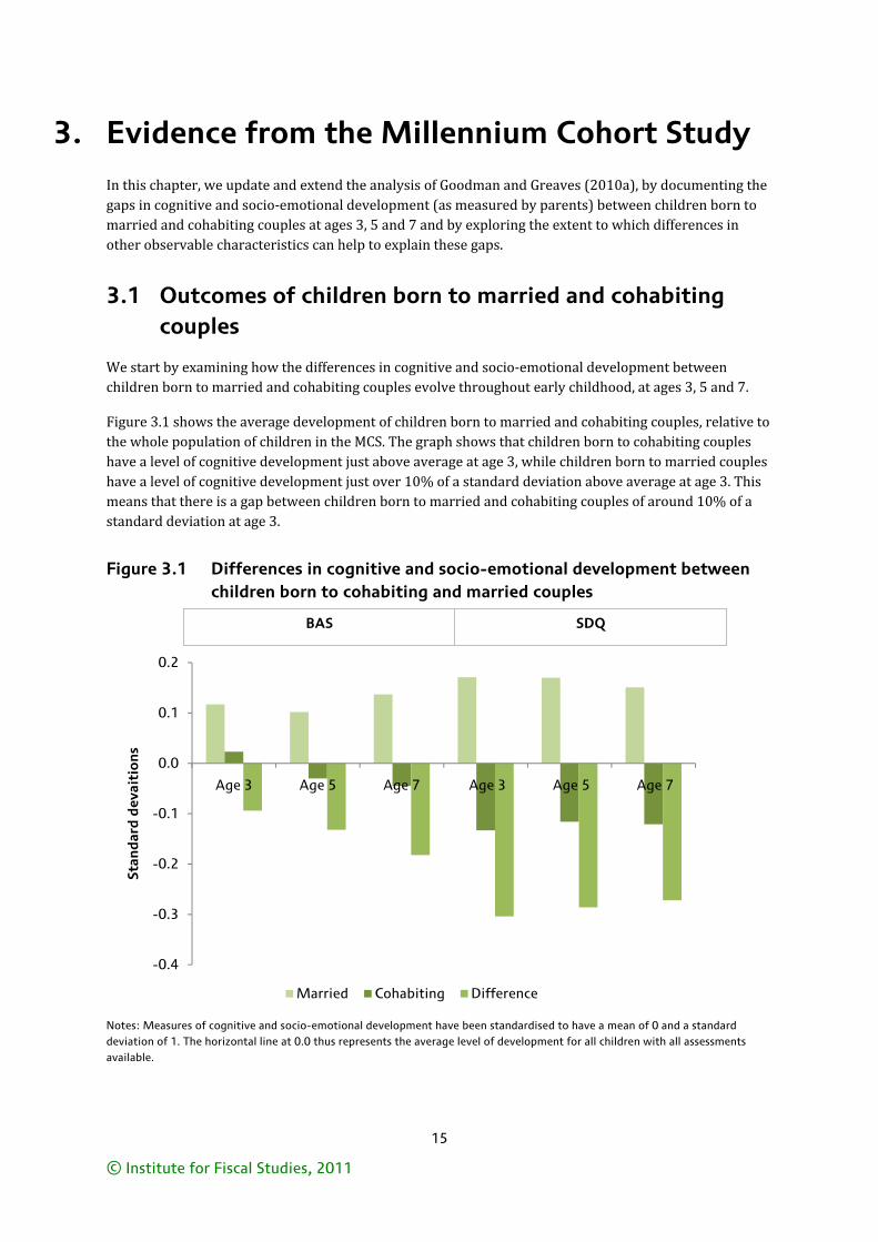
Figure 3.1 shows the average development of children born to married and cohabiting couples, relative to the whole population of children in the MCS. The graph shows that children born to cohabiting couples have a level of cognitive development just above average at age 3, while children born to married couples have a level of cognitive development just over 10% of a standard deviation above average at age 3. This means that there is a gap between children born to married and cohabiting couples of around 10% of a standard deviation at age 3.
Figure 3.1 Differences in cognitive and socio-emotional development between children born to cohabiting and married couples
Notes: Measures of cognitive and socio-emotional development have been standardised to have a mean of 0 and a standard deviation of 1. The horizontal line at 0.0 thus represents the average level of development for all children with all assessments available.
-0.4
-0.3
-0.2
-0.1
0.0
0.1
0.2
Age 3 Age 5 Age 7 Age 3 Age 5 Age 7
Stan
dar
d d
evai
tio
ns
Married Cohabiting Difference
BAS SDQ
Cohabitation, marriage, relationship stability and child outcomes: an update
16
© Institute for Fiscal Studies, 2011
Figure 3.1 also shows that children born to married parents have a level of socio-emotional development just over one-sixth of a standard deviation above average at age 3, while children born to cohabiting parents score just under one-sixth of a standard deviation below average. This implies a gap in development between children born to married and cohabiting couples of around one-third of a standard deviation at age 3, almost three times larger than the gap in cognitive development at the same age.
We can explore in more detail how these gaps evolve over time by considering Figures 3.2 and 3.3.
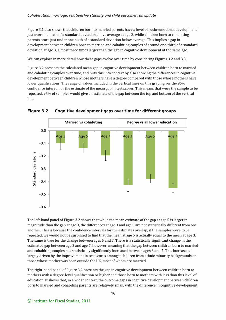
Figure 3.2 presents the calculated mean gap in cognitive development between children born to married and cohabiting couples over time, and puts this into context by also showing the differences in cognitive development between children whose mothers have a degree compared with those whose mothers have lower qualifications. The range of values included in the vertical lines on this graph gives the 95% confidence interval for the estimate of the mean gap in test scores. This means that were the sample to be repeated, 95% of samples would give an estimate of the gap between the top and bottom of the vertical line.
Figure 3.2 Cognitive development gaps over time for different groups
The left-hand panel of Figure 3.2 shows that while the mean estimate of the gap at age 5 is larger in magnitude than the gap at age 3, the differences at age 3 and age 5 are not statistically different from one another. This is because the confidence intervals for the estimates overlap; if the samples were to be repeated, we would not be surprised to find that the mean at age 5 is actually equal to the mean at age 3. The same is true for the change between ages 5 and 7. There is a statistically significant change in the estimated gap between age 3 and age 7, however, meaning that the gap between children born to married and cohabiting couples has statistically significantly increased between ages 3 and 7. This increase is largely driven by the improvement in test scores amongst children from ethnic minority backgrounds and those whose mother was born outside the UK, most of whom are married.
The right-hand panel of Figure 3.2 presents the gap in cognitive development between children born to mothers with a degree-level qualification or higher and those born to mothers with less than this level of education. It shows that, in a wider context, the outcome gaps in cognitive development between children born to married and cohabiting parents are relatively small, with the difference in cognitive development
-0.6
-0.5
-0.4
-0.3
-0.2
-0.1
0.0
Age 3 Age 5 Age 7 Age 3 Age 5 Age 7
Stan
dar
d d
evia
tio
ns
Mean Degree vs all lower education Married vs cohabiting
Evidence from the MCS
17
© Institute for Fiscal Studies, 2011
between children born to mothers with different levels of formal education just over 40% of a standard deviation at age 3, compared with under 10% of a standard deviation for the difference between children born to mothers in married and cohabiting relationships at the same age.
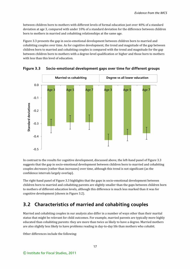
Figure 3.3 presents the gap in socio-emotional development between children born to married and cohabiting couples over time. As for cognitive development, the trend and magnitude of the gap between children born to married and cohabiting couples is compared with the trend and magnitude for the gap between children born to mothers with a degree-level qualification or higher and those born to mothers with less than this level of education.
Figure 3.3 Socio-emotional development gaps over time for different groups
In contrast to the results for cognitive development, discussed above, the left-hand panel of Figure 3.3 suggests that the gap in socio-emotional development between children born to married and cohabiting couples decreases (rather than increases) over time, although this trend is not significant (as the confidence intervals largely overlap).
The right-hand panel of Figure 3.3 highlights that the gaps in socio-emotional development between children born to married and cohabiting parents are slightly smaller than the gaps between children born to mothers of different education levels, although this difference is much less marked than it was for cognitive development (shown in Figure 3.2).
3.2 Characteristics of married and cohabiting couples
Married and cohabiting couples in our analysis also differ in a number of ways other than their marital status that might be relevant for child outcomes. For example, married parents are typically more highly educated than cohabiting parents: they are more than twice as likely to have a degree. Married mothers are also slightly less likely to have problems reading in day-to-day life than mothers who cohabit.
Other differences include the following:
-0.5
-0.4
-0.3
-0.2
-0.1
0.0
Age 3 Age 5 Age 7 Age 3 Age 5 Age 7
Stan
dar
d d
evia
tio
ns
Mean Degree vs all lower education Married vs cohabiting
Cohabitation, marriage, relationship stability and child outcomes: an update
18
© Institute for Fiscal Studies, 2011
• Fewer than 60% of mothers who are Black Caribbean are married when their child is born, compared with about 70% of mothers who are White. By contrast, almost all mothers who are Bangladeshi, Pakistani or Indian are married when their child is born.
• Mothers of all religious faiths are significantly more likely to be married than cohabiting compared with mothers of no religion.
• Married fathers are twice as likely as cohabiting fathers to have a professional occupation.
• Couples that are married typically have higher income than cohabiting couples: for example, at the time of their child’s birth, married couples are around twice as likely to be in the highest household income quintile and over three times less likely to be in the lowest household income quintile. Married couples are also more likely to own or have a mortgage for their home.
• Mothers in cohabiting couples are much more likely to have been a teenager at the time of their first child’s birth: 17% of mothers in cohabiting couples first gave birth before they were 20, compared with 4% of married mothers, while over 33% of married mothers were over 30 at the time of their first child’s birth, compared with 23% of cohabiting mothers.
• Married couples are much more likely to have lived together for a longer period of time prior to their child’s birth than cohabiting couples: over half of married couples have lived together for more than six years prior to the birth of the child in the MCS, compared with 16% of cohabiting couples. Almost 40% of cohabiting couples had lived together for less than two years, compared with only 8% of married couples.
• Mothers in married couples are much more likely to report that their pregnancy was planned; this was the case for 76% of married mothers compared with 49% of cohabiting mothers.
• There is some difference in ‘early’ relationship quality between married and cohabiting couples. When the child is 9 months old, 33% of married mothers report that their partner is usually sensitive and aware of their needs, compared with 28% of cohabiting mothers.23
It is clear from this analysis that there are large differences in observable characteristics, which are also likely to affect child development, between couples that are married and cohabiting when their child is born. In the next section, we attempt to take account of these differences in our analysis.
3.3 Regression results
In this section, we show how controlling for the differences in observable characteristics described above affects our estimates of the differences in cognitive and socio-emotional development between children born to married and cohabiting parents. Our intention in controlling for these observable characteristics is to control for selection into marriage as far as possible, without inadvertently controlling away any indirect effects of marriage on child development.
This selection of variables necessarily reflects some value judgement on our part, and we follow Goodman and Greaves (2010a) in this regard. They grouped observable characteristics into three categories:
1. fixed, or predetermined, characteristics that cannot be affected by marriage (exogenous variables); 2. characteristics that mainly reflect selection, but potentially capture causal pathways of marriage
(potentially endogenous variables); 3. characteristics that are possible causal pathways (potentially endogenous variables).
23 We refer the reader to chapter 4 of Goodman and Greaves (2010a) for further discussion of the differences in observable characteristics between couples that are married and couples that are cohabiting when their child is born.
19
© In
stit
ute
for
Fisc
al S
tudi
es, 2
01
1
Tab
le 3
.1
Dif
fere
nce
in c
og
nit
ive
and
so
cio
-em
oti
on
al d
evel
op
men
t at
ag
es 3
, 5
an
d 7
bet
wee
n c
hild
ren
bo
rn t
o c
oh
abit
ing
an
d m
arri
ed p
aren
ts
P
rede
term
ined
cha
ract
eris
tics
C
hara
cter
isti
cs m
ainl
y re
flec
ting
sel
ecti
on, b
ut p
oten
tial
ly c
aptu
ring
cau
sal p
athw
ays
A
R
aw
B
Eth
nici
ty
C
Mot
her’
s ba
ckgr
ound
D
Edu
cati
on
E
Occ
upat
ion
and
inco
me
F Fa
mily
ch
arac
teri
stic
s
G
Rel
atio
nshi
p qu
alit
y
Out
com
e va
riab
le
BA
S at
age
3
–0.0
94*
*
–0.1
37*
*
–0.0
93*
*
0.02
1
0.08
7**
0.
057
0.
061
BA
S at
age
5
–0.1
35*
*
–0.1
43*
*
–0.1
11*
*
–0.0
18
0.01
3
0.00
3
0.00
2
BA
S at
age
7
–0.1
89*
*
–0.1
70*
*
–0.1
41*
*
–0.0
36
0.00
2
0.00
3
0.00
6
SDQ
at
age
3
–0.3
14*
*
–0.3
00*
*
–0.2
70*
*
–0.1
79*
*
–0.1
13*
*
–0.0
62*
–0
.028
SDQ
at
age
5
–0.2
84*
*
–0.2
70*
*
–0.2
42*
*
–0.1
62*
*
–0.1
04*
*
–0.0
64*
–0
.026
SDQ
at
age
7
–0.2
74*
*
–0.2
64*
*
–0.2
30*
*
–0.1
54*
*
–0.0
91*
*
–0.0
38
–0.0
05
Chi
ld’s
gen
der
Y
es
Yes
Y
es
Yes
Y
es
Yes
Y
es
Chi
ld’s
yea
r a
nd
mon
th o
f b
irth
Y
es
Yes
Y
es
Yes
Y
es
Yes
Y
es
Mot
her’
s et
hnic
ity,
imm
igra
tion
sta
tus
and
rel
igio
n
No
Yes
Y
es
Yes
Y
es
Yes
Y
es
Mot
her
’s b
ack
gro
und
(ev
er in
ca
re,
pare
nts
sep
ara
ted
, pr
esen
ce o
f h
alf
- a
nd s
tep-
child
ren
whe
n th
e ch
ild is
b
orn,
hei
ght
)
No
No
Yes
Y
es
Yes
Y
es
Yes
Ed
uca
tion
N
o N
o N
o Y
es
Yes
Y
es
Yes
Fa
ther
’s o
ccup
ati
on,
hous
ehol
d
inco
me,
hou
sin
g t
enur
e a
nd p
are
nts’
w
ork
at
9 m
onth
s
No
No
No
No
Yes
Y
es
Yes
Fa
mily
str
uctu
re
No
No
No
No
No
Yes
Y
es
Rel
ati
onsh
ip q
ualit
y a
t 9
mon
ths
No
No
No
No
No
No
Yes
No.
of
obse
rva
tion
s 8
,56
2
8,5
62
8
,56
2
8,5
62
8
,56
2
8,5
62
8
,56
2
Not
es:
The
tabl
e sh
ows
reg
ress
ion
coef
fici
ents
on
a du
mm
y va
riab
le ‘b
iolo
gica
l par
ents
wer
e co
habi
ting
at
the
tim
e of
the
chi
ld’s
bir
th’;
the
om
itte
d g
roup
is t
here
fore
chi
ldre
n w
hose
bio
logi
cal p
aren
ts
wer
e m
arri
ed a
t th
e ti
me
of t
heir
bir
th. A
ll ot
her
coef
fici
ent
esti
mat
es a
re a
vaila
ble
on r
eque
st. A
co
mm
on
sam
ple
is u
sed
: th
ose
who
se b
iolo
gica
l par
ents
wer
e ei
ther
mar
ried
or
coha
biti
ng a
t th
e ti
me
of
thei
r b
irth
, and
who
are
in w
aves
1, 2
, 3 a
nd 4
of
the
MC
S an
d ha
ve n
on-m
issi
ng S
DQ
and
BA
S sc
ores
. Sta
ndar
d er
rors
are
clu
ster
ed b
y fa
mily
. * p
< 0
.05
, **
p <
0.0
1.
Cohabitation, marriage, relationship stability and child outcomes: an update
20
© Institute for Fiscal Studies, 2011
Each of these categories included up to a further four subdivisions, which allowed the authors to examine how controlling for these different sets of characteristics changed the estimated gap in development between children born to married and cohabiting couples. This approach allowed the reader to make a judgement about the extent to which the gap simply reflects ‘selection’ into marriage or is a causal effect of marriage on child development.
We follow their approach in this Commentary and we report our coefficient of interest – the ‘gap’ between children born to cohabiting and married parents – for seven model specifications, which sequentially include characteristics of the parents whose ‘exogeneity’ is increasingly questionable, because they might possibly be affected by marriage.
Our findings are based on the results from a set of simple regressions (estimated using ordinary least squares) in which the outcomes are our measures of the child’s cognitive or socio-emotional development at ages 3, 5 and 7. As all of our outcomes have been standardised, the regression coefficients are expressed in standard deviations.
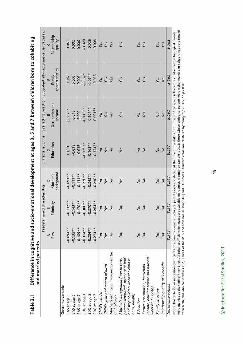
Table 3.1 shows only the estimated coefficients on the main variable of interest – a dummy variable (1–0 indicator) for whether or not the parents were cohabiting at the time of the child’s birth.24 Each row of the table shows estimated coefficients for a different outcome (e.g. cognitive development at age 3, socio-emotional development at age 5), while each column shows results from a different regression specification, when additional control variables are sequentially added to the model.
The first specification (shown in column A) includes only the dummy variable for whether the couple was married or cohabiting when the child was born, plus the child’s year and month of birth and gender. It therefore represents the ‘raw gap’ in development before we control for any observable characteristics of the parents. These gaps match those shown in Figures 3.2 and 3.325 and are all statistically significant.
The second and third specifications (columns B and C) add predetermined observable characteristics of the parents that cannot be affected by marriage, and therefore reflect only selection into marriage. Characteristics in this section include the mother’s ethnic group, religion and whether she was born outside the UK, whether the grandparents of the child were born outside the UK, and some other family history of the mother.
The fourth to seventh specifications (columns D to G) sequentially add potentially endogenous characteristics that we believe mainly reflect selection into marriage, but may also potentially capture causal pathways of marriage. These include the mother’s and father’s level of education, the father’s socio-economic classification of occupation, housing tenure, household income, employment status, the mother’s and father’s age at the birth of her/his first child, the length of the couple’s cohabitation prior to the birth of the child, whether the pregnancy was planned, and birth order of the child. The final specification (column G) includes a measure of relationship quality from wave 1 of the survey, soon after the child was born.26
In terms of cognitive development, we find that the biggest reduction in the estimated gap occurs once parental education is controlled for (see column D). In fact, the gap becomes small and statistically insignificant once we account for predetermined background characteristics of the mother and parental education. This suggests that the lower cognitive development of children born to cohabiting rather than married parents is largely accounted for by their parents’ lower education, and not by their parents’ marital status. There are many reasons why we might expect parents’ education to influence (or at least 24 Coefficient estimates for all other variables are available from the authors on request. 25 Although Figures 3.2 and 3.3 show the gap between children born to married and cohabiting couples before we control for the child’s month of birth and gender, this makes very little difference to the size of the ‘raw gap’. 26 A full description of the characteristics included in each group is given in Tables A.1 and A.2 of Appendix A.
Evidence from the MCS
21
© Institute for Fiscal Studies, 2011
be strongly correlated with) children’s development, but a full discussion of these issues is outside the scope of this Commentary. Nonetheless, we highlight three possibilities here as examples:
• Achieving a high level of education may increase access to resources or networks that could be used to improve children’s development.
• Parental education is likely to be highly correlated with cognitive ability. If we believe that cognitive ability is passed across generations either directly or indirectly, then we might expect it to be correlated with children’s development.
• Acquiring a high level of education may be a signal that the individual is willing to delay gratification to improve their later life. This characteristic may affect children’s development directly – for example, if the parent is willing to invest more in their young child – or indirectly – for example, if the parent is willing to delay having a child until they are ‘ready’.
Of course, it is possible that parental education decisions may be affected by the choice of whether or not to get married; however, it is our judgement that most people tend to have completed their education before making marriage decisions and, as such, that all of the variables included in our model at this point are largely predetermined, i.e. made before the decision to marry or cohabit. This suggests that selection plays a significant role in accounting for the difference in cognitive development between children of married and cohabiting couples, corroborating the findings of Goodman and Greaves (2010a).
In terms of socio-emotional development, the addition of controls for parental education and socio-economic status reduces (but does not entirely eliminate) the magnitude of the estimated gap between children born to married and cohabiting couples: it falls to just over half of the ‘raw’ difference once we add parental education (column D) and to around a third of the ‘raw’ difference once we add parents’ socio-economic status, occupation and income (column E). It is not until after we add controls for other characteristics of the family, including mother’s and father’s age when her/his first child was born, length of cohabitation prior to the birth of the child and whether the pregnancy was planned (column F) that the gap in socio-emotional development at age 7 (but not at ages 3 or 5) is entirely eliminated.
In column G, we additionally control for the quality of the relationship between the parents, which is self-reported by the mother when the baby is 9 months old. Our analysis reveals a strong positive association between parents’ relationship quality and children’s socio-emotional development.27 Since self-reported relationship quality is, on average, lower among cohabiting parents than among married parents, including this as a control reduces the estimated gap in socio-emotional outcomes between children born to cohabiting and married parents even further, such that it is no longer significant at any age.
Interestingly, our findings in terms of parent-reported socio-emotional development are corroborated by similar reports from teachers – see Table A.3 in Appendix A for details. This suggests that the difference observed in socio-emotional development between children born to married and cohabiting couples does not arise because these two groups of parents have different expectations about their children’s behaviour.28
It must be noted, however, that the differences in relationship quality (and other potentially endogenous variables) that we observe could arise both because happier couples make the decision to get married in the first place and because it is possible that marriage fosters a better relationship between parents. Since we cannot distinguish between these two explanations in the MCS data, we cannot be certain that by 27 See the coefficient in column 8, penultimate row, of Table A.4 in Appendix A. 28 Table A.3 also provides results for various other outcomes reported by the child’s teacher, including binary indicators for whether the child is assessed as above average in reading, writing and maths and whether the child has an emotional or behavioural difficulty, and a standardised continuous variable for their Foundation Stage Profile (FSP) score. All of these results suggest that the gap in outcomes between children born to cohabiting and married parents is driven largely by selection rather than being a causal effect of marriage itself.
Cohabitation, marriage, relationship stability and child outcomes: an update
22
© Institute for Fiscal Studies, 2011
controlling for these differences we are only removing the effects of selection from our estimates, and we therefore cannot claim to be estimating a true causal impact of marriage on child development. We return to this issue in the next chapter, which makes use of the BCS data.
3.4 Summary
Taken together, our findings confirm the broad conclusions reported in Goodman and Greaves (2010a):
• Children born to cohabiting parents exhibit a small but increasing deficit in cognitive development at ages 3, 5 and 7 compared with children born to married parents. This increasing gap in cognitive development is largely driven by the improvement in test scores amongst children from ethnic minority backgrounds and those whose mother was born outside the UK, most of whom are married.
• However, our results show that this deficit is largely accounted for by the fact that cohabiting parents have lower educational qualifications than married parents. While it is possible that the decision to be married might lead some parents to attain higher educational qualifications, this effect is likely to be small. Our judgement therefore is that the gap in cognitive development between children born to cohabiting compared with married parents is largely accounted for by their parents’ lower level of education, and is not a causal effect of their parents not being married.
• Children born to cohabiting parents exhibit a larger deficit in socio-emotional development (relative to cognitive development) at ages 3, 5 and 7 compared with children born to married parents. This gap is reduced by around two-thirds, but remains statistically significant, once differences in parental education and socio-economic status are controlled for. This suggests that the majority of the gap in socio-emotional development between children born to cohabiting as opposed to married parents is accounted for by their parents’ lower level of education and income.
• Once differences in family structure, including the likelihood of a pregnancy being unplanned and relationship quality when the child is 9 months old, are also controlled for, the gap in socio-emotional development between the children of married and cohabiting parents becomes even smaller, and is statistically insignificant.
• However, this analysis cannot perfectly distinguish the extent to which these differences reflect the sort of people who choose to marry in the first place and how much they are a positive product of marriage itself. The extent to which marriage fosters better relationship quality is perhaps the most debatable of these. This issue will be addressed in some detail in the BCS analysis in the next chapter.
23
© Institute for Fiscal Studies, 2011
4. Evidence from the British Cohort Study
The previous chapter argued that selection effects are likely to account for most or all of the differences in cognitive and socio-emotional development between children born to married and cohabiting couples. Indeed, for this not to be the case, it would need to be established that marriage leads to substantial improvements in parents’ education, occupation, income or relationship quality at the time children are 9 months old, and that this in turn leads to better outcomes for those children.
But the analysis in the previous chapter had an important limitation: the MCS data do not in general allow us to distinguish very well between factors that already differ between cohabiting and married couples when marriage decisions are made and factors that are themselves affected by marriage (except in particular cases – such as ethnicity – where characteristics are known to be predetermined). This is because the parents were first surveyed after their child was born (and hence after our marital status variable is defined). If some characteristics had already been affected by the decision of whether or not to marry, then controlling for them would necessarily involve ‘controlling away’ part of the effect of marriage. But not controlling for them would also very likely result in estimates of ‘marriage effects’ that were biased upwards due to selection.
In this chapter, we make use of a longitudinal survey, the BCS, which contains background information about one of the children’s parents from before their decision about whether to marry was taken. We can therefore be much surer that we are capturing only selection effects when such information is included in our model. In addition, we can account for things that were not available at all in the MCS data, such as parental cognitive and socio-emotional development (measured during the parent’s childhood). As we shall see, these additional factors are very important sources of selection into marriage. However, it must be remembered that the BCS data are not without their limitations: they have a relatively high attrition rate and only include children born to relatively young parents, one of whom was born in the UK, amongst other sample restrictions. Collectively, this means that it is a relatively unrepresentative sample of children in the UK. However, it is worth noting that our results do not materially change if we focus on the children of female cohort members only (whom we expect to be less affected by these restrictions).29
4.1 Outcomes of children born to married and cohabiting couples
Figure 4.1 shows the raw differences in cognitive and socio-emotional development between children born to married and cohabiting couples from the BCS.
As we would expect on the basis of the analysis of the previous chapter, Figure 4.1 shows that children born to married parents score better than children born to cohabiting parents on both measures: the gap is about 15% of a standard deviation for cognitive development and 18% of a standard deviation for socio-emotional development.30 The gap in cognitive development is similar to that found for children aged 3, 5 and 7 in the MCS, but the gap in socio-emotional development is somewhat smaller. This remains true when we compare children of a similar age, and when we restrict the MCS sample to children with at least one parent aged 27 to 31 when they were born and at least one parent born in the UK (which are conditions for inclusion in the BCS sample). See Table C.1 in Appendix C for full details of this analysis.
29 Compare the results shown in Table B.5 of Appendix B (for female cohort members only) with those shown in Table 4.2 (for all cohort members). 30 Note that there is no statistically significant difference between the parent-reported SDQ scores of children whose mother was questioned and those of children whose father was questioned. We thus report both together.
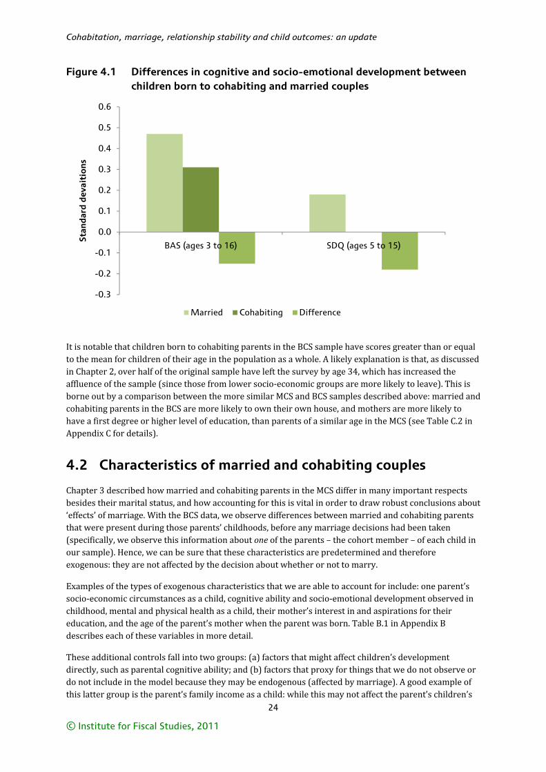
Cohabitation, marriage, relationship stability and child outcomes: an update
24
© Institute for Fiscal Studies, 2011
Figure 4.1 Differences in cognitive and socio-emotional development between children born to cohabiting and married couples
It is notable that children born to cohabiting parents in the BCS sample have scores greater than or equal to the mean for children of their age in the population as a whole. A likely explanation is that, as discussed in Chapter 2, over half of the original sample have left the survey by age 34, which has increased the affluence of the sample (since those from lower socio-economic groups are more likely to leave). This is borne out by a comparison between the more similar MCS and BCS samples described above: married and cohabiting parents in the BCS are more likely to own their own house, and mothers are more likely to have a first degree or higher level of education, than parents of a similar age in the MCS (see Table C.2 in Appendix C for details).
4.2 Characteristics of married and cohabiting couples
Chapter 3 described how married and cohabiting parents in the MCS differ in many important respects besides their marital status, and how accounting for this is vital in order to draw robust conclusions about ‘effects’ of marriage. With the BCS data, we observe differences between married and cohabiting parents that were present during those parents’ childhoods, before any marriage decisions had been taken (specifically, we observe this information about one of the parents – the cohort member – of each child in our sample). Hence, we can be sure that these characteristics are predetermined and therefore exogenous: they are not affected by the decision about whether or not to marry.
Examples of the types of exogenous characteristics that we are able to account for include: one parent’s socio-economic circumstances as a child, cognitive ability and socio-emotional development observed in childhood, mental and physical health as a child, their mother’s interest in and aspirations for their education, and the age of the parent’s mother when the parent was born. Table B.1 in Appendix B describes each of these variables in more detail.
These additional controls fall into two groups: (a) factors that might affect children’s development directly, such as parental cognitive ability; and (b) factors that proxy for things that we do not observe or do not include in the model because they may be endogenous (affected by marriage). A good example of this latter group is the parent’s family income as a child: while this may not affect the parent’s children’s
-0.3
-0.2
-0.1
0.0
0.1
0.2
0.3
0.4
0.5
0.6
BAS (ages 3 to 16) SDQ (ages 5 to 15)
Stan
dar
d d
evai
tio
ns
Married Cohabiting Difference
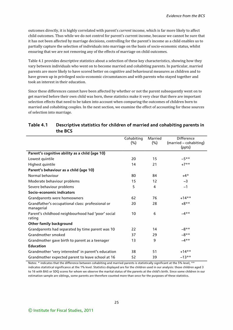
Evidence from the BCS
25
© Institute for Fiscal Studies, 2011
outcomes directly, it is highly correlated with parent’s current income, which is far more likely to affect child outcomes. Thus while we do not control for parent’s current income, because we cannot be sure that it has not been affected by marriage decisions, controlling for the parent’s income as a child enables us to partially capture the selection of individuals into marriage on the basis of socio-economic status, whilst ensuring that we are not removing any of the effects of marriage on child outcomes.
Table 4.1 provides descriptive statistics about a selection of these key characteristics, showing how they vary between individuals who went on to become married and cohabiting parents. In particular, married parents are more likely to have scored better on cognitive and behavioural measures as children and to have grown up in privileged socio-economic circumstances and with parents who stayed together and took an interest in their education.
Since these differences cannot have been affected by whether or not the parent subsequently went on to get married before their own child was born, these statistics make it very clear that there are important selection effects that need to be taken into account when comparing the outcomes of children born to married and cohabiting couples. In the next section, we examine the effect of accounting for these sources of selection into marriage.
Table 4.1 Descriptive statistics for children of married and cohabiting parents in the BCS
Cohabiting(%)
Married(%)
Difference(married – cohabiting)
(ppts)
Parent’s cognitive ability as a child (age 10)
Lowest quintile 20 15 –5**
Highest quintile 14 21 +7**
Parent’s behaviour as a child (age 10)
Normal behaviour 80 84 +4*
Moderate behaviour problems 15 12 –3
Severe behaviour problems 5 4 –1
Socio-economic indicators
Grandparents were homeowners 62 76 +14**
Grandfather’s occupational class: professional or managerial
20 28 +8**
Parent’s childhood neighbourhood had ‘poor’ social rating
10 6 –4**
Other family background
Grandparents had separated by time parent was 10 22 14 –8**
Grandmother smoked 37 29 –8**
Grandmother gave birth to parent as a teenager 13 9 –4**
Education
Grandmother ‘very interested’ in parent’s education 38 51 +14**
Grandmother expected parent to leave school at 16 52 39 –13**
Notes: * indicates that the difference between cohabiting and married parents is statistically significant at the 5% level; ** indicates statistical significance at the 1% level. Statistics displayed are for the children used in our analysis: those children aged 3 to 16 with BAS or SDQ scores for whom we observe the marital status of the parents at the child’s birth. Since some children in our estimation sample are siblings, some parents are therefore counted more than once for the purposes of these statistics.
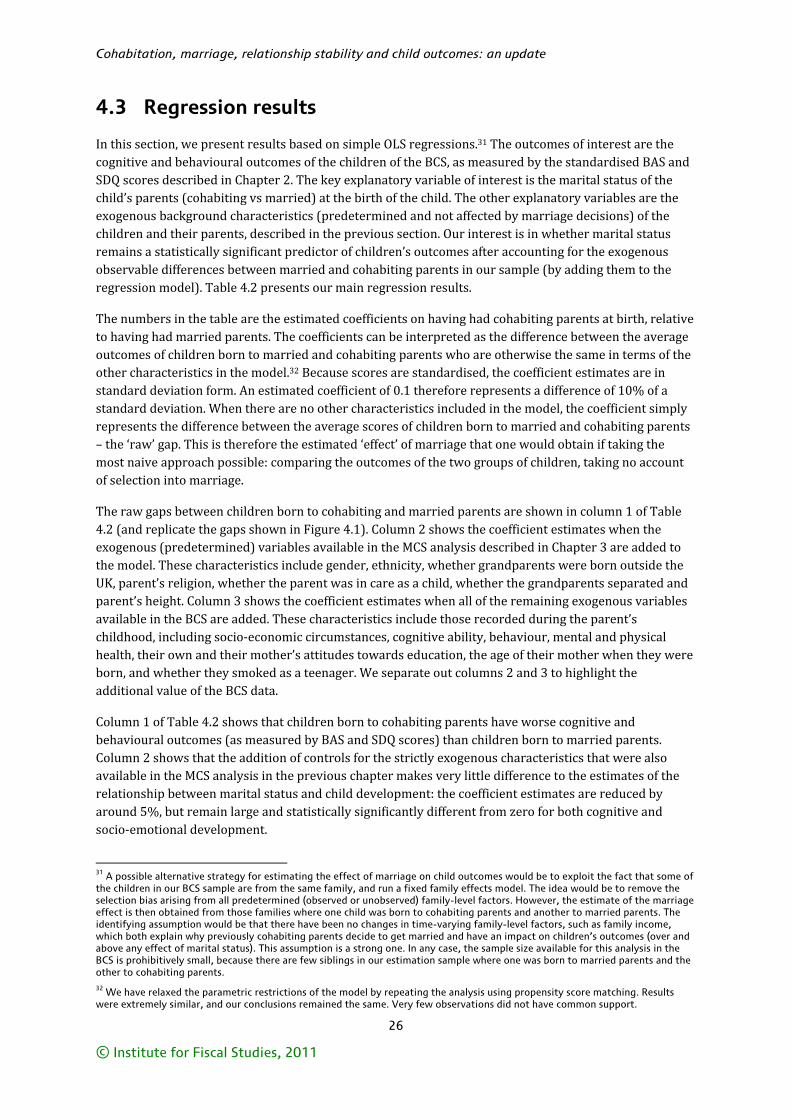
Cohabitation, marriage, relationship stability and child outcomes: an update
26
© Institute for Fiscal Studies, 2011
4.3 Regression results
In this section, we present results based on simple OLS regressions.31 The outcomes of interest are the cognitive and behavioural outcomes of the children of the BCS, as measured by the standardised BAS and SDQ scores described in Chapter 2. The key explanatory variable of interest is the marital status of the child’s parents (cohabiting vs married) at the birth of the child. The other explanatory variables are the exogenous background characteristics (predetermined and not affected by marriage decisions) of the children and their parents, described in the previous section. Our interest is in whether marital status remains a statistically significant predictor of children’s outcomes after accounting for the exogenous observable differences between married and cohabiting parents in our sample (by adding them to the regression model). Table 4.2 presents our main regression results.
The numbers in the table are the estimated coefficients on having had cohabiting parents at birth, relative to having had married parents. The coefficients can be interpreted as the difference between the average outcomes of children born to married and cohabiting parents who are otherwise the same in terms of the other characteristics in the model.32 Because scores are standardised, the coefficient estimates are in standard deviation form. An estimated coefficient of 0.1 therefore represents a difference of 10% of a standard deviation. When there are no other characteristics included in the model, the coefficient simply represents the difference between the average scores of children born to married and cohabiting parents – the ‘raw’ gap. This is therefore the estimated ‘effect’ of marriage that one would obtain if taking the most naive approach possible: comparing the outcomes of the two groups of children, taking no account of selection into marriage.
The raw gaps between children born to cohabiting and married parents are shown in column 1 of Table 4.2 (and replicate the gaps shown in Figure 4.1). Column 2 shows the coefficient estimates when the exogenous (predetermined) variables available in the MCS analysis described in Chapter 3 are added to the model. These characteristics include gender, ethnicity, whether grandparents were born outside the UK, parent’s religion, whether the parent was in care as a child, whether the grandparents separated and parent’s height. Column 3 shows the coefficient estimates when all of the remaining exogenous variables available in the BCS are added. These characteristics include those recorded during the parent’s childhood, including socio-economic circumstances, cognitive ability, behaviour, mental and physical health, their own and their mother’s attitudes towards education, the age of their mother when they were born, and whether they smoked as a teenager. We separate out columns 2 and 3 to highlight the additional value of the BCS data.
Column 1 of Table 4.2 shows that children born to cohabiting parents have worse cognitive and behavioural outcomes (as measured by BAS and SDQ scores) than children born to married parents. Column 2 shows that the addition of controls for the strictly exogenous characteristics that were also available in the MCS analysis in the previous chapter makes very little difference to the estimates of the relationship between marital status and child development: the coefficient estimates are reduced by around 5%, but remain large and statistically significantly different from zero for both cognitive and socio-emotional development.
31 A possible alternative strategy for estimating the effect of marriage on child outcomes would be to exploit the fact that some of the children in our BCS sample are from the same family, and run a fixed family effects model. The idea would be to remove the selection bias arising from all predetermined (observed or unobserved) family-level factors. However, the estimate of the marriage effect is then obtained from those families where one child was born to cohabiting parents and another to married parents. The identifying assumption would be that there have been no changes in time-varying family-level factors, such as family income, which both explain why previously cohabiting parents decide to get married and have an impact on children’s outcomes (over and above any effect of marital status). This assumption is a strong one. In any case, the sample size available for this analysis in the BCS is prohibitively small, because there are few siblings in our estimation sample where one was born to married parents and the other to cohabiting parents. 32 We have relaxed the parametric restrictions of the model by repeating the analysis using propensity score matching. Results were extremely similar, and our conclusions remained the same. Very few observations did not have common support.
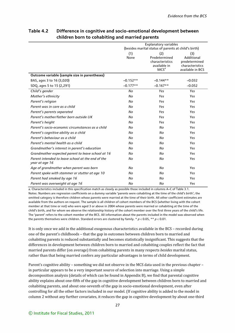
Evidence from the BCS
27
© Institute for Fiscal Studies, 2011
Table 4.2 Difference in cognitive and socio-emotional development between children born to cohabiting and married parents
Explanatory variables (besides marital status of parents at child’s birth)
(1) None
(2) Predetermined characteristics
available in MCSa
(3) Additional
predetermined characteristics
available in BCS
Outcome variable (sample size in parentheses)
BAS, ages 3 to 16 (3,020) –0.152** –0.144** –0.032
SDQ, ages 5 to 15 (2,291) –0.177** –0.167** –0.052
Child’s gender No Yes Yes
Mother’s ethnicity No Yes Yes
Parent’s religion No Yes Yes
Parent was in care as a child No Yes Yes
Parent’s parents separated No Yes Yes
Parent’s mother/father born outside UK No Yes Yes
Parent’s height No Yes Yes
Parent’s socio-economic circumstances as a child No No Yes
Parent’s cognitive ability as a child No No Yes
Parent’s behaviour as a child No No Yes
Parent’s mental health as a child No No Yes
Grandmother’s interest in parent’s education No No Yes
Grandmother expected parent to leave school at 16 No No Yes
Parent intended to leave school at the end of the year at age 16
No No Yes
Age of grandmother when parent was born No No Yes
Parent spoke with stammer or stutter at age 10 No No Yes
Parent had smoked by age 16 No No Yes
Parent was overweight at age 16 No No Yes
a. Characteristics included in this specification match as closely as possible those included in columns A–C of Table 3.1. Notes: Numbers are regression coefficients on a dummy variable ‘parents were cohabiting at the time of the child’s birth’; the omitted category is therefore children whose parents were married at the time of their birth. All other coefficient estimates are available from the authors on request. The sample is all children of cohort members of the BCS (whether living with the cohort member at that time or not) who were aged 3 or above in 2004 whose parents were married or cohabiting at the time of the child’s birth, and for whom we observe the relationship history of the cohort member over the first three years of the child’s life. The ‘parent’ refers to the cohort member of the BCS. All information about the parents included in the model was observed when the parents themselves were children. Standard errors are clustered by family. * p < 0.05, ** p < 0.01.
It is only once we add in the additional exogenous characteristics available in the BCS – recorded during one of the parent’s childhoods – that the gap in outcomes between children born to married and cohabiting parents is reduced substantially and becomes statistically insignificant. This suggests that the differences in development between children born to married and cohabiting couples reflect the fact that married parents differ (on average) from cohabiting parents in many respects besides marital status, rather than that being married confers any particular advantages in terms of child development.
Parent’s cognitive ability – something we did not observe in the MCS data used in the previous chapter – in particular appears to be a very important source of selection into marriage. Using a simple decomposition analysis (details of which can be found in Appendix B), we find that parental cognitive ability explains about one-fifth of the gap in cognitive development between children born to married and cohabiting parents, and about one-seventh of the gap in socio-emotional development, even after controlling for all the other factors included in our model. (If cognitive ability is added to the model in column 2 without any further covariates, it reduces the gap in cognitive development by about one-third
Cohabitation, marriage, relationship stability and child outcomes: an update
28
© Institute for Fiscal Studies, 2011
and the gap in socio-emotional development by about one-quarter.) For socio-emotional development, parent’s mental and physical health as a child also plays a significant role.
These results considerably strengthen the conclusions we were able to draw on the basis of the MCS analysis alone, because these characteristics are strictly exogenous – they are either fixed or were observed during the parent’s childhood, so cannot have been affected by the decision of whether or not to marry – so by including them in our model, we can be sure that we are only capturing the selection of individuals into marriage on the basis of these characteristics, while ensuring that we are not removing any of the effects of marriage on child outcomes.
It is worth noting that because the ‘effect’ of marital status on child development cannot now be distinguished from zero, there does not seem to be a need to go on to control for the types of characteristics included in columns D to G of the MCS analysis reported in Table 3.1, which could lead us to control away some of the effects of marriage on child development.
Readers interested in differences between particular subscales of the BAS cognitive tests or the SDQ measure of socio-emotional development should refer to Table B.2 in Appendix B, where we report the corresponding regression results for each of these subscales.33
4.4 Summary
The analysis in this chapter has strengthened the evidence presented in Chapter 3 that the differences in cognitive and socio-emotional development between children born to married and cohabiting parents mainly or entirely reflect selection effects, rather than effects of marital status on child development. We have been able to use information about one of the parents of the children in our sample observed during their own childhood, before marriage decisions were taken, enabling us to be sure that we are capturing selection effects rather than ‘controlling away’ any effects of marital status. After controlling for differences in other observable characteristics, we find no statistically significant difference between the cognitive and socio-emotional development of children born to married and cohabiting parents.
33 This exercise is problematic for components of the BAS scales, for the reasons outlined in footnote 22, and as such we do not discuss the results further. There are some interesting differences for different components of the SDQ scale, however, with a particularly large raw gap for conduct problems and a much smaller and insignificant gap in terms of emotional difficulties. For three out of the four components, the addition of controls for the full range of exogenous characteristics available in the BCS eliminates the vast majority of the raw gaps, suggesting that selection is playing a key role in driving these raw differences. In terms of conduct problems, however, the gap in outcomes between children born to married and cohabiting parents is substantially reduced, but remains significant, even after adding such controls. It is not clear what is driving these results.
29
© Institute for Fiscal Studies, 2011
5. Marital status, relationship stability and child outcomes
The evidence from Chapters 3 and 4 suggests that the gap in cognitive and socio-emotional development between children born to cohabiting and married couples is largely driven by selection – the fact that different types of parents choose to get married rather than cohabit – rather than being a large causal effect of marriage on child outcomes.
However, it is widely recognised that cohabiting parents are more likely to split up than married parents (Benson, 2009; Kiernan and Mensah, 2010) and that the outcomes for children whose parents separate are particularly poor. In our own previous work, we found that cohabiting parents were around four times more likely to have separated by the time the child was 3, and around three times more likely to have separated by the time the child was 5, than married parents (Goodman and Greaves, 2010b). Moreover, we found that children’s cognitive development and emotional well-being were, on average, very low among those children whose parents had split up.
In this chapter, we investigate two related issues: first, whether there is any evidence that marriage is the cause of this disparity in relationship stability (Section 5.2); and second, whether relationship breakdown amongst cohabiting couples leads to poorer outcomes for their children, compared with children of married parents, over and above the effects of differences in other observable characteristics (Section 5.3).
The approach we adopt mimics that in the previous chapters: we consider the extent to which differences in other observable characteristics between cohabiting and married parents can help to explain the gap in the likelihood of separation. We note that this type of analysis is not perfectly suited to the question at hand: relationship stability is also likely to be affected by shocks to the couple’s environment – for example, redundancy – which we would ideally model jointly with relationship separation. It also seems likely that some of the characteristics of the parents that we cannot observe – such as love and commitment – are more likely to affect the probability of separation than children’s outcomes. Nonetheless, we feel it is still useful to consider the extent to which observed differences between married and cohabiting couples can help to explain differences in the likelihood of separation.
5.1 Measuring relationship stability
In addition to classifying parents according to their marital status at birth, we are also able to classify them according to their relationship status when the child is aged 3 in both the MCS and the BCS, and additionally at ages 5 and 7 in the MCS. In the MCS, we use information available from the household grid,34 while in the BCS, we use information about relationship histories that we have constructed, based partially on the relationship histories file. In both cases, we are able to consider whether parents have separated or, for cohabiting parents only, remained cohabiting or got married during the child’s early life.
Table 5.1 shows that 24% of cohabiting parents in the MCS have experienced a period of separation before their child’s 3rd birthday, compared with 6% of married parents. These figures are slightly higher
34 The household grid contains a record of all people in the household and each person’s relationship to the child and to all other members in the household. From this, we can look at how many biological parents of the child are in the household. If two biological parents are present in the household, then we can also look at their marital status – for example, ‘spouse’ or ‘partner’. We also check our definition of household status when the child is aged 7 by corroborating with other questions in the survey. For example, some questions are asked only to main respondents with a partner in the household and some questions are only relevant to those who have got married.
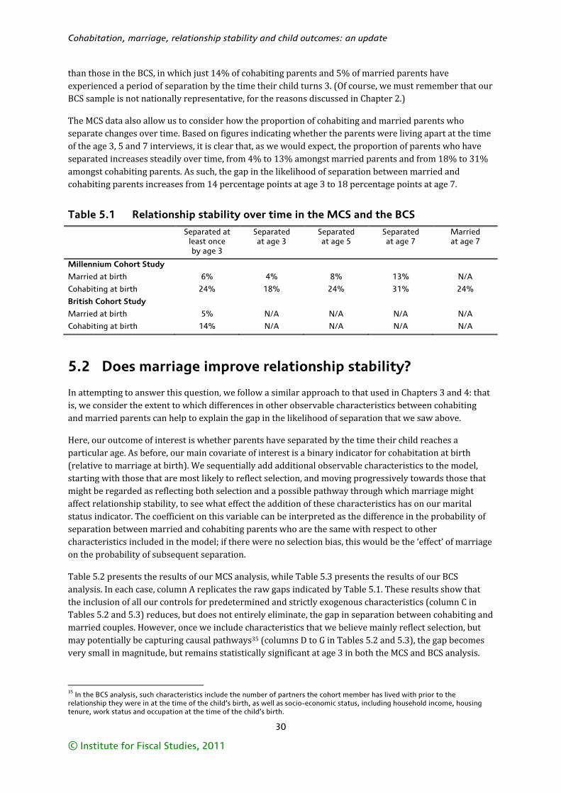
Cohabitation, marriage, relationship stability and child outcomes: an update
30
© Institute for Fiscal Studies, 2011
than those in the BCS, in which just 14% of cohabiting parents and 5% of married parents have experienced a period of separation by the time their child turns 3. (Of course, we must remember that our BCS sample is not nationally representative, for the reasons discussed in Chapter 2.)
The MCS data also allow us to consider how the proportion of cohabiting and married parents who separate changes over time. Based on figures indicating whether the parents were living apart at the time of the age 3, 5 and 7 interviews, it is clear that, as we would expect, the proportion of parents who have separated increases steadily over time, from 4% to 13% amongst married parents and from 18% to 31% amongst cohabiting parents. As such, the gap in the likelihood of separation between married and cohabiting parents increases from 14 percentage points at age 3 to 18 percentage points at age 7.
Table 5.1 Relationship stability over time in the MCS and the BCS
Separated at least once by age 3
Separated at age 3
Separated at age 5
Separated at age 7
Married at age 7
Millennium Cohort Study
Married at birth 6% 4% 8% 13% N/A
Cohabiting at birth 24% 18% 24% 31% 24%
British Cohort Study
Married at birth 5% N/A N/A N/A N/A
Cohabiting at birth 14% N/A N/A N/A N/A
5.2 Does marriage improve relationship stability?
In attempting to answer this question, we follow a similar approach to that used in Chapters 3 and 4: that is, we consider the extent to which differences in other observable characteristics between cohabiting and married parents can help to explain the gap in the likelihood of separation that we saw above.
Here, our outcome of interest is whether parents have separated by the time their child reaches a particular age. As before, our main covariate of interest is a binary indicator for cohabitation at birth (relative to marriage at birth). We sequentially add additional observable characteristics to the model, starting with those that are most likely to reflect selection, and moving progressively towards those that might be regarded as reflecting both selection and a possible pathway through which marriage might affect relationship stability, to see what effect the addition of these characteristics has on our marital status indicator. The coefficient on this variable can be interpreted as the difference in the probability of separation between married and cohabiting parents who are the same with respect to other characteristics included in the model; if there were no selection bias, this would be the ‘effect’ of marriage on the probability of subsequent separation.
Table 5.2 presents the results of our MCS analysis, while Table 5.3 presents the results of our BCS analysis. In each case, column A replicates the raw gaps indicated by Table 5.1. These results show that the inclusion of all our controls for predetermined and strictly exogenous characteristics (column C in Tables 5.2 and 5.3) reduces, but does not entirely eliminate, the gap in separation between cohabiting and married couples. However, once we include characteristics that we believe mainly reflect selection, but may potentially be capturing causal pathways35 (columns D to G in Tables 5.2 and 5.3), the gap becomes very small in magnitude, but remains statistically significant at age 3 in both the MCS and BCS analysis.
35 In the BCS analysis, such characteristics include the number of partners the cohort member has lived with prior to the relationship they were in at the time of the child’s birth, as well as socio-economic status, including household income, housing tenure, work status and occupation at the time of the child’s birth.
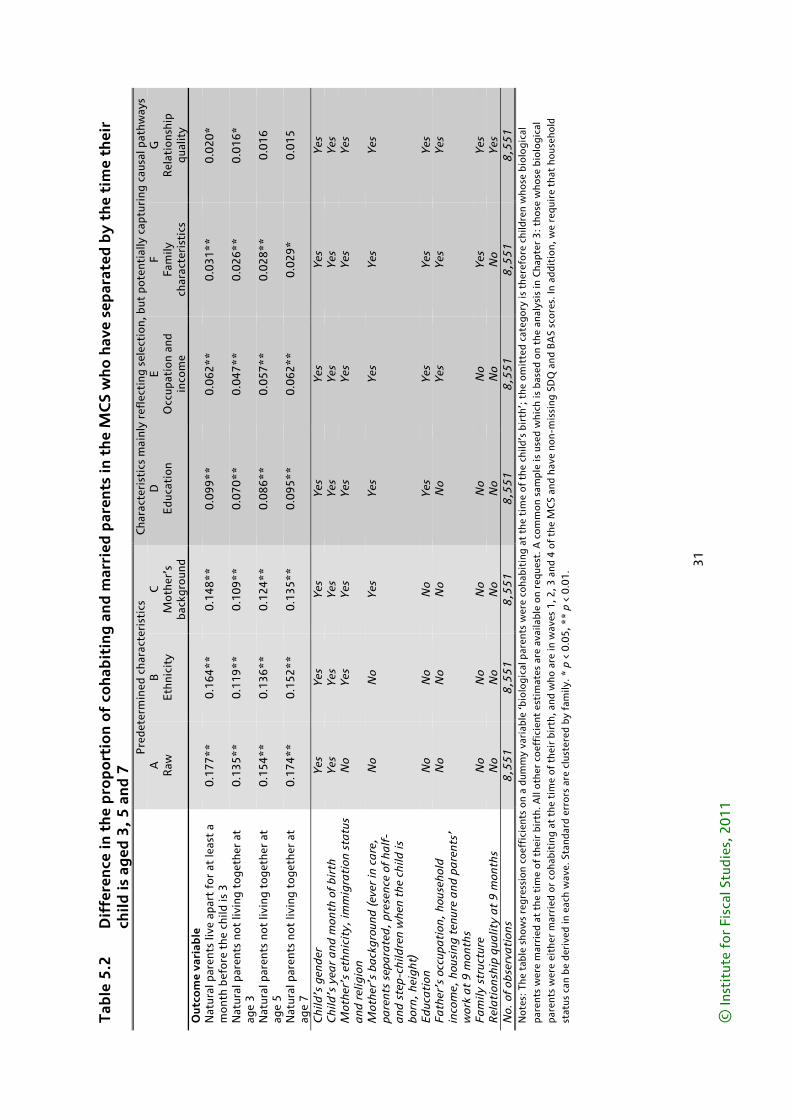
31
© In
stit
ute
for
Fisc
al S
tudi
es, 2
01
1
Tab
le 5
.2
Dif
fere
nce
in t
he
pro
po
rtio
n o
f co
hab
itin
g a
nd
mar
ried
par
ents
in t
he
MC
S w
ho
hav
e se
par
ated
by
the
tim
e th
eir
child
is a
ged
3,
5 a
nd
7
P
rede
term
ined
cha
ract
eris
tics
C
hara
cter
isti
cs m
ainl
y re
flec
ting
sel
ecti
on, b
ut p
oten
tial
ly c
aptu
ring
cau
sal p
athw
ays
A
R
aw
B
Eth
nici
ty
C
Mot
her’
s ba
ckgr
ound
D
Edu
cati
on
E
Occ
upat
ion
and
inco
me
F Fa
mily
ch
arac
teri
stic
s
G
Rel
atio
nshi
p qu
alit
y O
utco
me
vari
able
Nat
ural
par
ents
live
apa
rt f
or a
t le
ast
a m
onth
bef
ore
the
child
is 3
0.
177*
*
0.16
4**
0.
148*
*
0.09
9**
0.
062*
*
0.03
1**
0.
020*
Nat
ural
par
ents
not
livi
ng t
oget
her
at
age
3
0.13
5**
0.
119*
*
0.10
9**
0.
070*
*
0.04
7**
0.
026*
*
0.01
6*
Nat
ural
par
ents
not
livi
ng t
oget
her
at
age
5
0.15
4**
0.
136*
*
0.12
4**
0.
086*
*
0.05
7**
0.
028*
*
0.01
6
Nat
ural
par
ents
not
livi
ng t
oget
her
at
age
7
0.17
4**
0.
152*
*
0.13
5**
0.
095*
*
0.06
2**
0.
029*
0.
015
Chi
ld’s
gen
der
Y
es
Yes
Y
es
Yes
Y
es
Yes
Y
es
Chi
ld’s
yea
r a
nd
mon
th o
f b
irth
Y
es
Yes
Y
es
Yes
Y
es
Yes
Y
es
Mot
her’
s et
hnic
ity,
imm
igra
tion
sta
tus
and
rel
igio
n
No
Yes
Y
es
Yes
Y
es
Yes
Y
es
Mot
her
’s b
ack
gro
und
(ev
er in
ca
re,
pare
nts
sep
ara
ted
, pr
esen
ce o
f h
alf
- a
nd s
tep-
child
ren
whe
n th
e ch
ild is
b
orn,
hei
ght
)
No
No
Yes
Y
es
Yes
Y
es
Yes
Ed
uca
tion
N
o N
o N
o Y
es
Yes
Y
es
Yes
F
ath
er’s
occ
upa
tion
, ho
useh
old
in
com
e, h
ousi
ng
ten
ure
and
pa
rent
s’
wor
k a
t 9
mon
ths
No
No
No
No
Yes
Y
es
Yes
Fa
mily
str
uctu
re
No
No
No
No
No
Yes
Y
es
Rel
ati
onsh
ip q
ualit
y a
t 9
mon
ths
No
No
No
No
No
No
Yes
N
o. o
f ob
serv
ati
ons
8,5
51
8
,55
1
8,5
51
8
,55
1
8,5
51
8
,55
1
8,5
51
N
otes
: Th
e ta
ble
show
s re
gre
ssio
n co
effi
cien
ts o
n a
dum
my
vari
able
‘bio
logi
cal p
aren
ts w
ere
coha
biti
ng a
t th
e ti
me
of t
he c
hild
’s b
irth
’; t
he o
mit
ted
cate
gory
is t
here
fore
chi
ldre
n w
hose
bio
logi
cal
pare
nts
wer
e m
arri
ed a
t th
e ti
me
of
thei
r bi
rth.
All
oth
er c
oeff
icie
nt e
stim
ates
are
ava
ilabl
e on
req
uest
. A c
omm
on s
ampl
e is
use
d w
hich
is b
ased
on
the
anal
ysis
in C
hapt
er 3
: th
ose
who
se b
iolo
gica
l pa
rent
s w
ere
eith
er m
arri
ed o
r co
habi
ting
at
the
tim
e of
the
ir b
irth
, and
who
are
in w
aves
1, 2
, 3 a
nd 4
of
the
MC
S an
d ha
ve n
on-m
issi
ng S
DQ
and
BA
S sc
ore
s. In
add
itio
n, w
e re
qui
re t
hat
hous
ehol
d st
atus
can
be
deri
ved
in e
ach
wav
e. S
tand
ard
erro
rs a
re c
lust
ered
by
fam
ily. *
p <
0.0
5, *
* p
< 0
.01
.
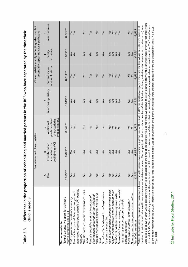
32
© In
stit
ute
for
Fisc
al S
tudi
es, 2
01
1
Tab
le 5
.3
Dif
fere
nce
in t
he
pro
po
rtio
n o
f co
hab
itin
g a
nd
mar
ried
par
ents
in t
he
BC
S w
ho
hav
e se
par
ated
by
the
tim
e th
eir
child
is a
ged
3
Not
es:
The
tabl
e sh
ows
reg
ress
ion
coef
fici
ents
on
a du
mm
y va
riab
le ‘p
aren
ts w
ere
coha
biti
ng a
t th
e ti
me
of t
he c
hild
’s b
irth
’; t
he o
mit
ted
cate
gory
is t
here
fore
chi
ldre
n w
hose
par
ents
wer
e m
arri
ed a
t th
e ti
me
of t
heir
bir
th. A
ll ot
her
coef
fici
ent
esti
mat
es a
re a
vaila
ble
on r
eque
st. T
he s
ampl
e is
all
child
ren
of c
ohor
t m
embe
rs o
f th
e B
CS
(whe
ther
livi
ng w
ith
the
coho
rt m
emb
er a
t th
at t
ime
or
not)
who
w
ere
aged
3 o
r ab
ove
in 2
00
4 w
hose
par
ents
wer
e m
arri
ed o
r co
habi
ting
at
the
tim
e o
f th
e ch
ild’s
bir
th, a
nd f
or w
hom
we
obse
rve
the
rela
tion
ship
his
tory
of
the
coho
rt m
embe
r ov
er t
he f
irst
thr
ee y
ears
of
the
chi
ld’s
life
. We
incl
ude
dum
my
vari
able
s fo
r th
e ye
ar in
whi
ch t
he c
hild
tur
ned
3 t
o ta
ke a
ccou
nt o
f th
e fa
ct t
hat
the
prob
abili
ty o
f p
aren
tal s
epar
atio
n ha
s in
crea
sed
over
tim
e. T
he ‘p
aren
t’ r
efer
s to
the
coh
ort
mem
ber
of t
he B
CS.
All
info
rmat
ion
abou
t th
e p
aren
ts in
clud
ed in
the
mo
del w
as o
bser
ved
whe
n th
e pa
rent
s th
emse
lves
wer
e ch
ildre
n. S
tand
ard
erro
rs a
re c
lust
ered
by
fam
ily. *
p <
0.0
5,
**
p <
0.0
1.
P
rede
term
ined
cha
ract
eris
tics
Cha
ract
eris
tics
mai
nly
refl
ecti
ng s
elec
tion
, but
po
tent
ially
cap
turi
ng c
ausa
l pat
hway
s
A
Raw
B
P
rede
term
ined
ch
arac
teri
stic
s av
aila
ble
in M
CS
C
Add
itio
nal
pred
eter
min
ed
char
acte
rist
ics
avai
labl
e in
BC
S
D
Rel
atio
nshi
p hi
stor
y E
C
urre
nt s
ocio
-ec
onom
ic s
tatu
s
F Fa
mily
st
ruct
ure
G
Yea
r du
mm
ies
Out
com
e va
riab
le
N
atur
al p
aren
ts li
ve a
part
for
at
leas
t a
mon
th b
efor
e th
e ch
ild is
3
0.08
9**
0.
078*
*
0.06
8**
0.
049*
*
0.03
4**
0.
033*
*
0.02
9**
Chi
ld’s
gen
der
and
mot
her’
s et
hnic
ity
No
Yes
Y
es
Yes
Y
es
Yes
Y
es
Pa
rent
’s b
ack
gro
und
(ev
er in
ca
re,
pare
nts
sepa
rate
d,
pare
nts
bor
n ou
tsid
e U
K,
heig
ht,
relig
ion)
No
No
Yes
Y
es
Yes
Y
es
Yes
Pa
rent
’s s
ocio
-eco
nom
ic c
ircu
mst
anc
es a
s a
ch
ild
No
No
Yes
Y
es
Yes
Y
es
Yes
Pa
rent
’s c
ogni
tive
and
soc
io-e
mot
iona
l d
evel
opm
ent
obse
rved
dur
ing
chi
ldho
od
No
No
Yes
Y
es
Yes
Y
es
Yes
Pa
rent
’s m
enta
l and
phy
sica
l hea
lth
as
a
child
N
o N
o Y
es
Yes
Y
es
Yes
Y
es
Gra
ndm
othe
r’s
inte
rest
in a
nd
asp
ira
tion
s fo
r pa
rent
’s e
duc
ati
on
No
No
Yes
Y
es
Yes
Y
es
Yes
Ag
e of
gra
ndm
othe
r w
hen
pare
nt w
as
bor
n
No
No
Yes
Y
es
Yes
Y
es
Yes
Le
ngth
of
coha
bit
ati
on b
efor
e b
irth
of
child
N
o N
o N
o Y
es
Yes
Y
es
Yes
N
umb
er o
f pa
rtne
rs p
revi
ousl
y liv
ed w
ith
N
o N
o N
o Y
es
Yes
Y
es
Yes
H
ouse
hold
inco
me,
hou
sing
ten
ure,
pa
rent
s’
wor
k st
atu
s a
nd
occ
upa
tion
at
bir
th,
pare
nts’
ed
uca
tion
No
No
No
No
Yes
Y
es
Yes
Bir
th o
rder
, m
ulti
ple-
bir
th in
dic
ato
r N
o N
o N
o N
o N
o Y
es
Yes
D
umm
y va
ria
ble
s fo
r ye
ar
of o
bse
rva
tion
N
o N
o N
o N
o N
o N
o Y
es
No.
of
obse
rva
tion
s 6
,92
3
6,9
23
6
,92
3
6,9
23
6
,92
3
6,9
23
6
,92
3
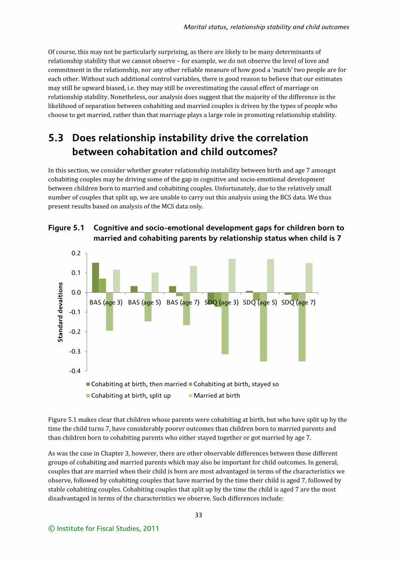
Marital status, relationship stability and child outcomes
33
© Institute for Fiscal Studies, 2011
Of course, this may not be particularly surprising, as there are likely to be many determinants of relationship stability that we cannot observe – for example, we do not observe the level of love and commitment in the relationship, nor any other reliable measure of how good a ‘match’ two people are for each other. Without such additional control variables, there is good reason to believe that our estimates may still be upward biased, i.e. they may still be overestimating the causal effect of marriage on relationship stability. Nonetheless, our analysis does suggest that the majority of the difference in the likelihood of separation between cohabiting and married couples is driven by the types of people who choose to get married, rather than that marriage plays a large role in promoting relationship stability.
5.3 Does relationship instability drive the correlation between cohabitation and child outcomes?
In this section, we consider whether greater relationship instability between birth and age 7 amongst cohabiting couples may be driving some of the gap in cognitive and socio-emotional development between children born to married and cohabiting couples. Unfortunately, due to the relatively small number of couples that split up, we are unable to carry out this analysis using the BCS data. We thus present results based on analysis of the MCS data only.
Figure 5.1 Cognitive and socio-emotional development gaps for children born to married and cohabiting parents by relationship status when child is 7
Figure 5.1 makes clear that children whose parents were cohabiting at birth, but who have split up by the time the child turns 7, have considerably poorer outcomes than children born to married parents and than children born to cohabiting parents who either stayed together or got married by age 7.
As was the case in Chapter 3, however, there are other observable differences between these different groups of cohabiting and married parents which may also be important for child outcomes. In general, couples that are married when their child is born are most advantaged in terms of the characteristics we observe, followed by cohabiting couples that have married by the time their child is aged 7, followed by stable cohabiting couples. Cohabiting couples that split up by the time the child is aged 7 are the most disadvantaged in terms of the characteristics we observe. Such differences include:
-0.4
-0.3
-0.2
-0.1
0.0
0.1
0.2
BAS (age 3) BAS (age 5) BAS (age 7) SDQ (age 3) SDQ (age 5) SDQ (age 7)
Stan
dar
d d
evai
tio
ns
Cohabiting at birth, then married Cohabiting at birth, stayed so
Cohabiting at birth, split up Married at birth
Cohabitation, marriage, relationship stability and child outcomes: an update
34
© Institute for Fiscal Studies, 2011
• Around 35% of mothers who are married when their child is born have a degree, compared with 18% of cohabiting mothers who decide to get married by the time the child is aged 7. In comparison, less than 10% of mothers who are cohabiting when the child is born but have split up from their partner by the time the child is 7 have a degree.
• Married fathers are four times as likely to have a professional occupation as cohabiting fathers who split up by the time their child is 7.
• Couples that are married at the time of their child’s birth are around four times as likely to be in the highest household income quintile as couples that are cohabiting at the time of their child’s birth and then separate by the time the child is 7.
• Nearly 27% of mothers in cohabiting couples that split up were teenagers at the time of their first child’s birth, compared with 14% of mothers in cohabiting couples that stay together and 9% of mothers in cohabiting couples that get married.
• About 17% of couples that were cohabiting when their child was born but split up by the time the child is 7 had lived together for less than 9 months before their child was born. Less than 1% of married couples had lived together for less than 9 months before their child was born.
• Mothers in married couples are much more likely to report that their pregnancy was planned; this was the case for 76% of married mothers compared with just over half of cohabiting mothers who decide to get married or remain cohabiting and for under 40% of cohabiting mothers who have split up by the time the child is 7.
• There is some difference in ‘early’ relationship quality between married and cohabiting couples in different circumstances. When the child is 9 months old, 32% of married mothers report that their partner is usually sensitive and aware of their needs, compared with fewer than 20% of cohabiting mothers who separate by the time the child is 7. Interestingly, 37% of cohabiting mothers who decide to get married agree (when the child is 9 months) that their partner is usually sensitive and aware of their needs – a higher proportion than for mothers who were married when their child was born.
A full set of descriptive characteristics is provided in Table D.1 in Appendix D.
With these differences in mind, we now move on to consider the extent to which the raw gaps in cognitive and socio-emotional development between children born to cohabiting and married parents can be explained by differences in other observable characteristics, using a simple regression framework similar to that used in Chapters 3 and 4. Here, the main coefficients of interest are indicators of whether a child’s parents were:
i) cohabiting at birth but got married by the time the child turned 7; ii) cohabiting at birth and remained so when the child turned 7; iii) cohabiting at birth but split up by the time the child turned 7.
Couples that were married when their child was born, regardless of whether they split up by the time the child is aged 7, remain the base group.36 This allows us to decompose the coefficient on the cohabiting indicator variable shown in Table 3.1 into the average effect for each of these subgroups.
36 We have also examined an alternative specification in which we restrict the base group to ‘stable married parents’, i.e. those children whose parents were married at birth and remained so by the age of 7. In this specification, we added a dummy for having married parents who had split up by the age of 7. While this approach additionally highlighted the negative association between marital breakdown and children’s outcomes, it did not substantively alter any of the findings outlined in this section. Detailed results are available on request.

35
© In
stit
ute
for
Fisc
al S
tudi
es, 2
01
1
Tab
le 5
.4
Dif
fere
nce
in c
og
nit
ive
and
so
cio
-em
oti
ona
l dev
elo
pm
ent
at a
ges
3, 5
and
7 b
etw
een
child
ren
bo
rn t
o m
arri
ed a
nd c
oh
abit
ing
par
ents
of
dif
fere
nt
mar
ital
sta
tes
wh
en t
he
child
is a
ged
7
P
rede
term
ined
cha
ract
eris
tics
C
hara
cter
isti
cs m
ainl
y re
flec
ting
sel
ecti
on, b
ut p
oten
tial
ly c
aptu
ring
ca
usal
pat
hway
s
A
R
aw
B
Eth
nici
ty
C
Mot
her’
s ba
ckgr
ound
D
Edu
cati
on
E
Occ
upat
ion
and
inco
me
F Fa
mily
ch
arac
teri
stic
s
G
Rel
atio
nshi
p qu
alit
y O
utco
me
vari
able
BA
S at
age
3:
Coh
abit
ing
at b
irth
, got
mar
ried
0.
052
–0
.003
0.
038
0.
095*
0.
111*
0.
079
0.
075
Coh
abit
ing
at b
irth
, sta
yed
so
–0.0
44
–0.0
91*
–0
.050
0.
050
0.
105*
*
0.07
0
0.07
4
C
ohab
itin
g at
bir
th, s
plit
up
–0.2
98*
*
–0.3
33*
*
–0.2
81*
*
–0.1
07*
0.
024
–0
.004
0.
008
BA
S at
age
5:
Coh
abit
ing
at b
irth
, got
mar
ried
–0
.068
–0
.087
*
–0.0
57
–0.0
01
0.00
7
0.00
3
0.00
2
C
ohab
itin
g at
bir
th, s
taye
d so
–0
.099
**
–0
.112
**
–0
.083
**
0.
002
0.
028
0.
011
0.
010
Coh
abit
ing
at b
irth
, spl
it u
p –0
.247
**
–0
.242
**
–0
.205
**
–0
.068
*
–0.0
08
–0.0
18
–0.0
18
BA
S at
age
7:
Coh
abit
ing
at b
irth
, got
mar
ried
–0
.106
**
–0
.099
**
–0
.072
–0
.010
0.
003
0.
010
0.
009
Coh
abit
ing
at b
irth
, sta
yed
so
–0.1
60*
*
–0.1
45*
*
–0.1
19*
*
–0.0
22
0.01
0
0.00
4
0.00
7
C
ohab
itin
g at
bir
th, s
plit
up
–0.3
02*
*
–0.2
72*
*
–0.2
37*
*
–0.0
83*
–0
.012
–0
.009
–0
.001
SDQ
at
age
3:
Coh
abit
ing
at b
irth
, got
mar
ried
–0
.224
**
–0
.222
**
–0
.194
**
–0
.145
**
–0
.124
**
–0
.078
–0
.092
Coh
abit
ing
at b
irth
, sta
yed
so
–0.2
55*
*
–0.2
42*
*
–0.2
15*
*
–0.1
34*
*
–0.0
79*
–0
.041
–0
.001
Coh
abit
ing
at b
irth
, spl
it u
p –0
.489
**
–0
.467
**
–0
.435
**
–0
.295
**
–0
.170
**
–0
.088
–0
.002
SDQ
at
age
5:
Coh
abit
ing
at b
irth
, got
mar
ried
–0
.162
**
–0
.162
**
–0
.135
**
–0
.091
–0
.071
–0
.040
–0
.055
Coh
abit
ing
at b
irth
, sta
yed
so
–0.2
04*
*
–0.1
95*
*
–0.1
69*
*
–0.1
00*
*
–0.0
55
–0.0
30
0.01
4
C
ohab
itin
g at
bir
th, s
plit
up
–0.5
21*
*
–0.4
96*
*
–0.4
68*
*
–0.3
53*
*
–0.2
49*
*
–0.1
94*
*
–0.1
01
SDQ
at
age
7:
Coh
abit
ing
at b
irth
, got
mar
ried
–0
.161
**
–0
.161
**
–0
.130
**
–0
.092
–0
.073
–0
.031
–0
.044
Coh
abit
ing
at b
irth
, sta
yed
so
–0.1
88*
*
–0.1
81*
*
–0.1
50*
*
–0.0
85*
–0
.034
0.
004
0.
043
Coh
abit
ing
at b
irth
, spl
it u
p –0
.503
**
–0
.486
**
–0
.449
**
–0
.338
**
–0
.224
**
–0
.151
**
–0
.070
C
hild
’s g
end
er
-Yes
-Y
es
-Yes
-Y
es
-Yes
-Y
es
-Yes
C
hild
’s y
ear
an
d m
onth
of
bir
th
-Yes
-Y
es
-Yes
-Y
es
-Yes
-Y
es
-Yes
M
othe
r’s
ethn
icit
y, im
mig
rati
on s
tatu
s a
nd r
elig
ion
-No
-Yes
-Y
es
-Yes
-Y
es
-Yes
-Y
es
Mot
her’
s b
ack
gro
und
(ev
er in
ca
re,
pare
nts
sepa
rate
d,
pres
ence
of
half
- a
nd s
tep-
child
ren
whe
n th
e ch
ild is
b
orn,
hei
ght
)
-No
-No
-Yes
-Y
es
-Yes
-Y
es
-Yes
Ed
uca
tion
-N
o -N
o -N
o -Y
es
-Yes
-Y
es
-Yes
F
ath
er’s
occ
upa
tion
, ho
useh
old
inco
me,
hou
sing
te
nure
and
pa
rent
s’ w
ork
at
9 m
onth
s -N
o -N
o -N
o -N
o -Y
es
-Yes
-Y
es
Fa
mily
str
uctu
re
-No
-No
-No
-No
-No
-Yes
-Y
es
Rel
ati
onsh
ip q
ualit
y a
t 9
mon
ths
-No
-No
-No
-No
-No
-No
-Yes
N
o. o
f ob
serv
ati
ons
8,5
62
8
,56
2
8,5
62
8
,56
2
8,5
62
8
,56
2
8,5
62
N
otes
: Th
e ta
ble
show
s re
gre
ssio
n co
effi
cien
ts o
n a
dum
my
vari
able
‘bio
logi
cal p
aren
ts w
ere
coha
biti
ng a
t th
e ti
me
of t
he c
hild
’s b
irth
’; t
he o
mit
ted
gro
up is
the
refo
re c
hild
ren
who
se b
iolo
gica
l par
ents
w
ere
mar
ried
at
the
tim
e of
the
ir b
irth
. All
othe
r co
effi
cien
t es
tim
ates
are
ava
ilabl
e on
req
uest
. A c
om
mo
n sa
mp
le is
use
d:
tho
se w
hose
bio
logi
cal p
aren
ts w
ere
eith
er m
arri
ed o
r co
habi
ting
at
the
tim
e of
the
ir b
irth
, and
who
are
in w
aves
1, 2
, 3 a
nd 4
of
the
MC
S an
d ha
ve n
on-m
issi
ng S
DQ
and
BA
S sc
ore
s. In
add
itio
n, w
e re
quir
e th
at h
ous
ehol
d st
atus
can
be
deri
ved
in e
ach
wav
e. S
tand
ard
erro
rs a
re
clus
tere
d by
fam
ily. *
p <
0.0
5, *
* p
< 0
.01
.
Cohabitation, marriage, relationship stability and child outcomes: an update
36
© Institute for Fiscal Studies, 2011
Table 5.4 presents the results of this analysis. It shows that controlling for observable characteristics (columns B–G) reveals a story very similar to that described in Chapter 3:
• All differences in cognitive development between children born to married couples and those born to cohabiting couples within each of the three subgroups identified above become small and insignificant (or, occasionally, positive and significant) once measures of parental education and socio-economic status are added into the model (columns D and E).
• Differences in socio-emotional development are reduced, but remain significant, after controlling for parental education and socio-economic status (columns D and E). They are further reduced, and become statistically insignificant, by the addition of controls for family structure and relationship quality (columns F and G). This is the case even among the subgroup of children born to cohabiting parents who subsequently split up, where the ‘raw’ outcome gaps were particularly large.
5.4 Summary
This chapter has shown the following:
• Cohabiting parents are more likely to split up by the time their child turns 3 than married parents. However, this gap is almost entirely eliminated after accounting for other observable characteristics that we believe wholly or largely reflect selection. This suggests that the vast majority of the raw gap in the likelihood of separation between cohabiting and married couples is driven by the selection of different types of people into marriage, rather than by a causal effect of marriage on relationship stability.
• Moreover, while cohabiting couples are more likely to separate than married ones, this does not appear to have a detrimental effect on their children’s cognitive or socio-emotional development, once we have taken account of the other ways in which cohabiting and married couples differ. This is the case even among the group of children born to cohabiting parents who subsequently split up, where the ‘raw’ outcome gaps are particularly large. As with the analysis in Chapters 3 and 4, this suggests that marriage does not have a causal effect on child outcomes.
37
© Institute for Fiscal Studies, 2011
6. Conclusions
The Prime Minister, David Cameron, has repeatedly expressed his desire to support marriage through the tax system. Most recently, in an article in the Sunday Telegraph on 19 June 2011, he wrote: ‘I want us to recognise marriage in the tax system so as a country we show we value commitment’.37 This desire is presumably at least partly based on a belief that such family situations are better for children along a number of dimensions.
This Commentary has considered the evidence for such beliefs, by examining the impact of marriage on relationship stability and child outcomes. It has done so using the simple regression approach adopted by Goodman and Greaves (2010a), of sequentially controlling for other ways in which married and cohabiting parents differ – starting with those that are most likely to reflect selection into marriage, and moving progressively towards those that might be regarded as reflecting both selection and a possible pathway through which marriage might have a causal effect – to see what the addition of these characteristics does to the ‘impact’ of marriage on child development.
We find the following:
• Children born to cohabiting parents exhibit a small deficit in cognitive development and a slightly larger deficit in socio-emotional development compared with children born to married parents. This is true at ages 3, 5 and 7 in the Millennium Cohort Study and over a broader span of ages in the British Cohort Study.
• Cohabiting couples are more likely to have split up by the time their child turns 7 than married parents (although this is largely driven by differences in other observable characteristics between cohabiting and married parents). The gaps in development between children born to cohabiting and married parents are much larger for the children of cohabiting parents who subsequently split up.
• These gaps in development are substantially reduced by the inclusion of predetermined (entirely exogenous) characteristics in the MCS, and entirely eliminated by the inclusion of the richer set of exogenous characteristics – including parental cognitive ability, plus various details of the parents’ own childhood, including socio-economic status, physical and mental health, and their own parents’ attitudes and aspirations – in the BCS analysis. In fact, we find that cognitive ability directly explains about one-fifth of the gap in outcomes between children born to cohabiting and married parents.
Taken together, these findings support the broad conclusions reported in Goodman and Greaves (2010a and 2010b) and suggest that the gaps in cognitive and socio-emotional development between children born to married and cohabiting parents mainly or entirely reflect the fact that different types of people choose to get married (the selection effect), rather than that marriage itself has a direct effect on relationship stability or child development.
On the basis of this evidence, therefore, there does not seem to be a strong reason in terms of child development for policymakers to encourage parents to get married before they bear children. There is, however, good reason for policymakers to continue to try to increase the educational attainment of today’s children (tomorrow’s parents) as a means of improving the outcomes of future generations of children.
37 See http://www.telegraph.co.uk/news/politics/david-cameron/8584238/David-Cameron-Dads-gift-to-me-was-his-optimism.html.
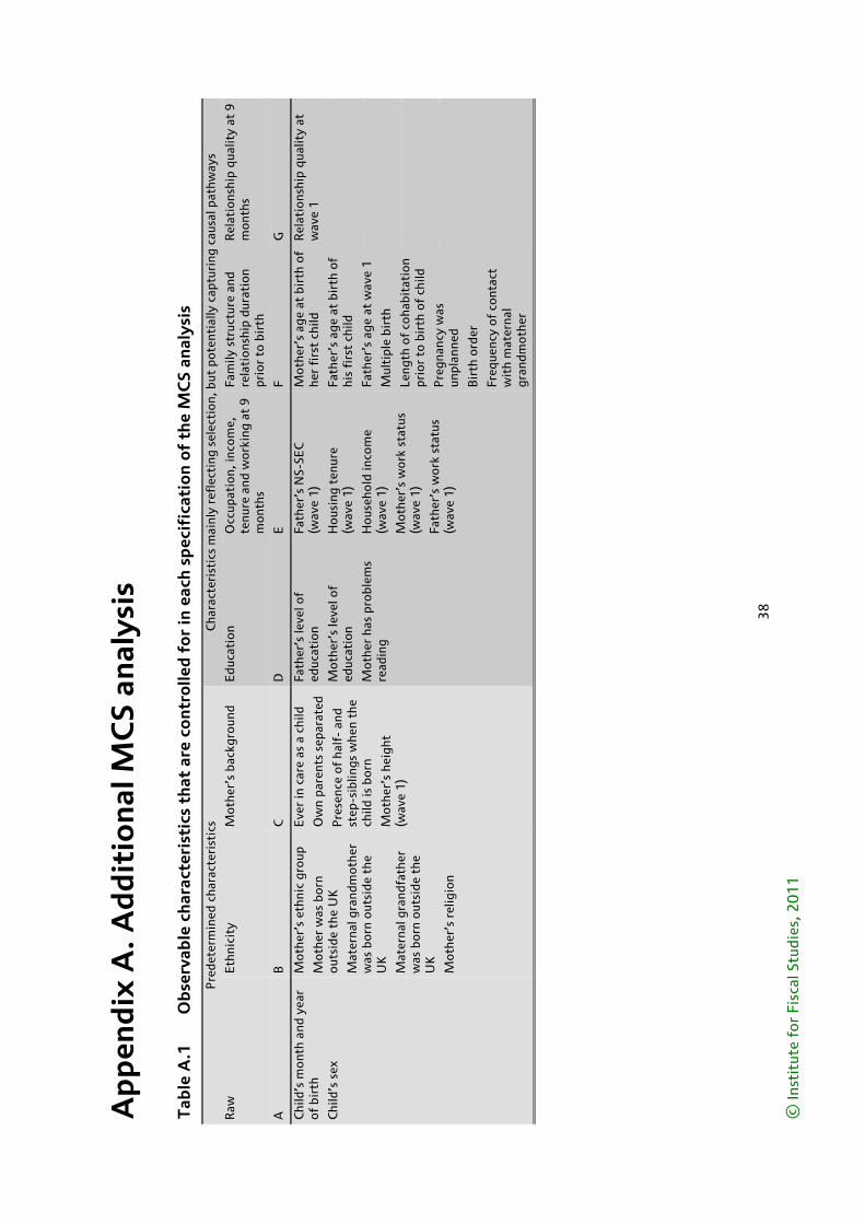
38
© In
stit
ute
for
Fisc
al S
tudi
es, 2
01
1
Ap
pen
dix
A. A
dd
itio
nal
MC
S an
alys
is
Tab
le A
.1
Ob
serv
able
ch
arac
teri
stic
s th
at a
re c
on
tro
lled
fo
r in
eac
h s
pec
ific
atio
n o
f th
e M
CS
anal
ysis
Pre
dete
rmin
ed c
hara
cter
isti
cs
Cha
ract
eris
tics
mai
nly
refl
ecti
ng s
elec
tion
, but
pot
enti
ally
cap
turi
ng c
ausa
l pat
hway
s
Raw
E
thni
city
M
othe
r’s
back
grou
nd
Edu
cati
on
Occ
upat
ion,
inco
me,
te
nure
and
wor
king
at
9
mon
ths
Fam
ily s
truc
ture
and
re
lati
onsh
ip d
urat
ion
prio
r to
bir
th
Rel
atio
nshi
p qu
alit
y at
9
mon
ths
A
B
C
D
E
F G
Chi
ld’s
mon
th a
nd y
ear
of b
irth
Chi
ld’s
sex
Mot
her’
s et
hnic
gro
up
Mot
her
was
bor
n ou
tsid
e th
e U
K
Mat
erna
l gra
ndm
othe
r w
as b
orn
outs
ide
the
UK
Mat
erna
l gra
ndfa
ther
w
as b
orn
outs
ide
the
UK
Mot
her’
s re
ligio
n
Eve
r in
car
e as
a c
hild
Ow
n pa
rent
s se
para
ted
Pre
senc
e of
hal
f- a
nd
step
-sib
lings
whe
n th
e ch
ild is
bor
n
Mot
her’
s he
ight
(w
ave
1)
Fath
er’s
leve
l of
educ
atio
n
Mot
her’
s le
vel o
f ed
ucat
ion
Mot
her
has
pro
blem
s re
adin
g
Fath
er’s
NS-
SEC
(w
ave
1)
Hou
sing
ten
ure
(wav
e 1)
Hou
seho
ld in
com
e (w
ave
1)
Mot
her’
s w
ork
stat
us
(wav
e 1)
Fath
er’s
wor
k st
atus
(w
ave
1)
Mot
her’
s ag
e at
bir
th o
f he
r fi
rst
child
Fath
er’s
age
at
birt
h of
hi
s fi
rst
child
Fath
er’s
age
at
wav
e 1
Mul
tipl
e bi
rth
Leng
th o
f co
habi
tati
on
prio
r to
bir
th o
f ch
ild
Pre
gnan
cy w
as
unpl
anne
d
Bir
th o
rder
Freq
uenc
y of
con
tact
w
ith
mat
erna
l gr
andm
othe
r
Rel
atio
nshi
p qu
alit
y at
w
ave
1
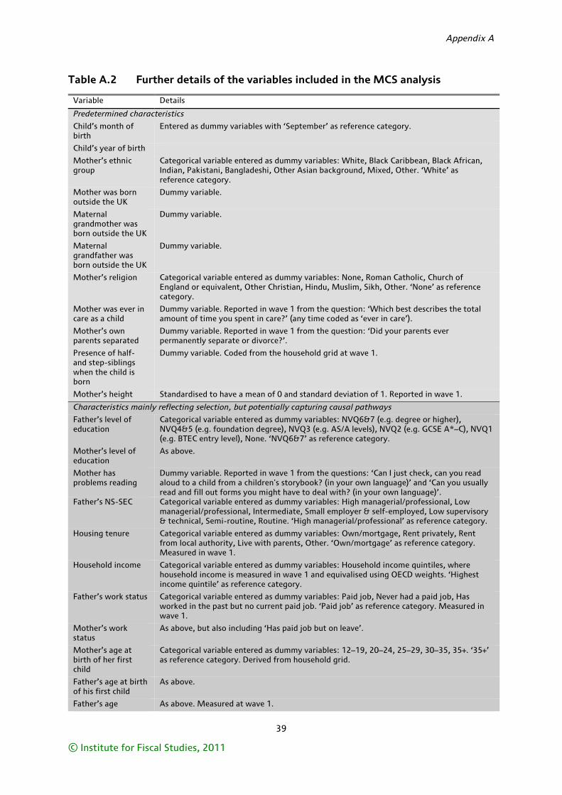
Appendix A
39
© Institute for Fiscal Studies, 2011
Table A.2 Further details of the variables included in the MCS analysis
Variable Details
Predetermined characteristics
Child’s month of birth
Entered as dummy variables with ‘September’ as reference category.
Child’s year of birth
Mother’s ethnic group
Categorical variable entered as dummy variables: White, Black Caribbean, Black African, Indian, Pakistani, Bangladeshi, Other Asian background, Mixed, Other. ‘White’ as reference category.
Mother was born outside the UK
Dummy variable.
Maternal grandmother was born outside the UK
Dummy variable.
Maternal grandfather was born outside the UK
Dummy variable.
Mother’s religion Categorical variable entered as dummy variables: None, Roman Catholic, Church of England or equivalent, Other Christian, Hindu, Muslim, Sikh, Other. ‘None’ as reference category.
Mother was ever in care as a child
Dummy variable. Reported in wave 1 from the question: ‘Which best describes the total amount of time you spent in care?’ (any time coded as ‘ever in care’).
Mother’s own parents separated
Dummy variable. Reported in wave 1 from the question: ‘Did your parents ever permanently separate or divorce?’.
Presence of half- and step-siblings when the child is born
Dummy variable. Coded from the household grid at wave 1.
Mother’s height Standardised to have a mean of 0 and standard deviation of 1. Reported in wave 1.
Characteristics mainly reflecting selection, but potentially capturing causal pathways
Father’s level of education
Categorical variable entered as dummy variables: NVQ6&7 (e.g. degree or higher), NVQ4&5 (e.g. foundation degree), NVQ3 (e.g. AS/A levels), NVQ2 (e.g. GCSE A*–C), NVQ1 (e.g. BTEC entry level), None. ‘NVQ6&7’ as reference category.
Mother’s level of education
As above.
Mother has problems reading
Dummy variable. Reported in wave 1 from the questions: ‘Can I just check, can you read aloud to a child from a children's storybook? (in your own language)’ and ‘Can you usually read and fill out forms you might have to deal with? (in your own language)’.
Father’s NS-SEC Categorical variable entered as dummy variables: High managerial/professional, Low managerial/professional, Intermediate, Small employer & self-employed, Low supervisory & technical, Semi-routine, Routine. ‘High managerial/professional’ as reference category.
Housing tenure Categorical variable entered as dummy variables: Own/mortgage, Rent privately, Rent from local authority, Live with parents, Other. ‘Own/mortgage’ as reference category. Measured in wave 1.
Household income Categorical variable entered as dummy variables: Household income quintiles, where household income is measured in wave 1 and equivalised using OECD weights. ‘Highest income quintile’ as reference category.
Father’s work status Categorical variable entered as dummy variables: Paid job, Never had a paid job, Has worked in the past but no current paid job. ‘Paid job’ as reference category. Measured in wave 1.
Mother’s work status
As above, but also including ‘Has paid job but on leave’.
Mother’s age at birth of her first child
Categorical variable entered as dummy variables: 12–19, 20–24, 25–29, 30–35, 35+. ‘35+’ as reference category. Derived from household grid.
Father’s age at birth of his first child
As above.
Father’s age As above. Measured at wave 1.
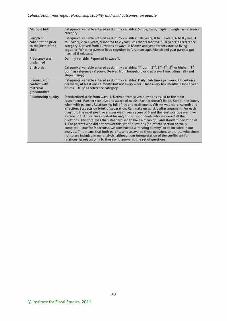
Cohabitation, marriage, relationship stability and child outcomes: an update
40
© Institute for Fiscal Studies, 2011
Multiple birth Categorical variable entered as dummy variables: Single, Twin, Triplet. ‘Single’ as reference category.
Length of cohabitation prior to the birth of the child
Categorical variable entered as dummy variables: 10+ years, 8 to 10 years, 6 to 8 years, 4 to 6 years, 2 to 4 years, 9 months to 2 years, less than 9 months. ‘10+ years’ as reference category. Derived from questions at wave 1: Month and year parents started living together, Whether parents lived together before marriage, Month and year parents got married if relevant.
Pregnancy was unplanned
Dummy variable. Reported in wave 1.
Birth order Categorical variable entered as dummy variables: 1st born, 2nd, 3rd, 4th, 5th or higher. ‘1st born’ as reference category. Derived from household grid at wave 1 (including half- and step-siblings).
Frequency of contact with maternal grandmother
Categorical variable entered as dummy variables: Daily, 3–6 times per week, Once/twice per week, At least once a month but not every week, Once every few months, Once a year or less. ‘Daily’ as reference category.
Relationship quality Standardised scale from wave 1. Derived from seven questions asked to the main respondent: Partner sensitive and aware of needs, Partner doesn’t listen, Sometimes lonely when with partner, Relationship full of joy and excitement, Wishes was more warmth and affection, Suspects on brink of separation, Can make up quickly after argument. For each question, the most positive answer was given a score of 6 and the least positive was given a score of 1. A total was created for only those respondents who answered all the questions. This total was then standardised to have a mean of 0 and standard deviation of 1. For parents who did not answer this set of questions (or left the section partially complete – true for 9 parents), we constructed a ‘missing dummy’ to be included in our analysis. This means that both parents who answered these questions and those who chose not to are included in our analysis, although our interpretation of the coefficient for relationship relates only to those who answered the set of questions.
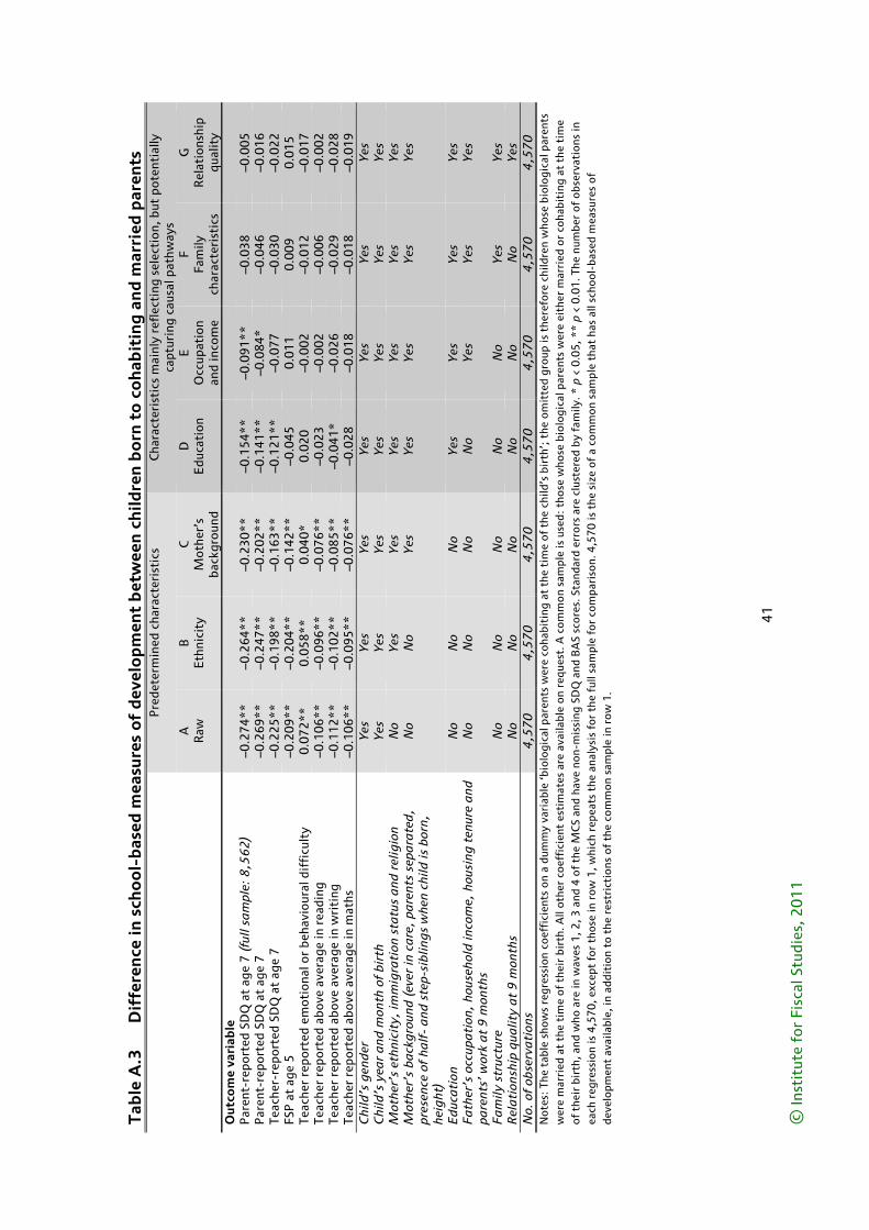
41
© In
stit
ute
for
Fisc
al S
tudi
es, 2
01
1
Tab
le A
.3
Dif
fere
nce
in s
cho
ol-
bas
ed m
easu
res
of
dev
elo
pm
ent
bet
wee
n c
hild
ren
bo
rn t
o c
oh
abit
ing
an
d m
arri
ed p
aren
ts
P
rede
term
ined
cha
ract
eris
tics
C
hara
cter
isti
cs m
ainl
y re
flec
ting
sel
ecti
on, b
ut p
oten
tial
ly
capt
urin
g ca
usal
pat
hway
s
A
R
aw
B
Eth
nici
ty
C
Mot
her’
s ba
ckgr
ound
D
Edu
cati
on
E
Occ
upat
ion
and
inco
me
F Fa
mily
ch
arac
teri
stic
s
G
Rel
atio
nshi
p qu
alit
y O
utco
me
vari
able
Par
ent-
repo
rted
SD
Q a
t ag
e 7
(ful
l sa
mpl
e: 8
,56
2)
–0.2
74*
*
–0.2
64*
*
–0.2
30*
*
–0.1
54*
*
–0.0
91*
*
–0.0
38
–0.0
05
Par
ent-
repo
rted
SD
Q a
t ag
e 7
–0
.269
**
–0
.247
**
–0
.202
**
–0
.141
**
–0
.084
*
–0.0
46
–0.0
16
Teac
her-
repo
rted
SD
Q a
t ag
e 7
–0
.225
**
–0
.198
**
–0
.163
**
–0
.121
**
–0
.077
–0
.030
–0
.022
FS
P a
t ag
e 5
–0
.209
**
–0
.204
**
–0
.142
**
–0
.045
0.
011
0.
009
0.
015
Te
ache
r re
port
ed e
mot
iona
l or
beha
viou
ral d
iffi
cult
y 0.
072*
*
0.05
8**
0.
040*
0.
020
–0
.002
–0
.012
–0
.017
Te
ache
r re
port
ed a
bove
ave
rage
in r
eadi
ng
–0.1
06*
*
–0.0
96*
*
–0.0
76*
*
–0.0
23
–0.0
02
–0.0
06
–0.0
02
Teac
her
repo
rted
abo
ve a
vera
ge in
wri
ting
–0
.112
**
–0
.102
**
–0
.085
**
–0
.041
*
–0.0
26
–0.0
29
–0.0
28
Teac
her
repo
rted
abo
ve a
vera
ge in
mat
hs
–0.1
06*
*
–0.0
95*
*
–0.0
76*
*
–0.0
28
–0.0
18
–0.0
18
–0.0
19
Chi
ld’s
gen
der
Y
es
Yes
Y
es
Yes
Y
es
Yes
Y
es
Chi
ld’s
yea
r a
nd
mon
th o
f b
irth
Y
es
Yes
Y
es
Yes
Y
es
Yes
Y
es
Mot
her’
s et
hnic
ity,
imm
igra
tion
sta
tus
and
rel
igio
n N
o Y
es
Yes
Y
es
Yes
Y
es
Yes
M
othe
r’s
ba
ckg
roun
d (
ever
in c
are
, pa
rent
s se
para
ted
, pr
esen
ce o
f ha
lf-
and
ste
p-si
blin
gs
whe
n ch
ild is
bor
n,
hei
gh
t)
No
No
Yes
Y
es
Yes
Y
es
Yes
Ed
uca
tion
N
o N
o N
o Y
es
Yes
Y
es
Yes
F
ath
er’s
occ
upa
tion
, ho
useh
old
inco
me,
hou
sing
ten
ure
an
d
pare
nts’
wor
k a
t 9
mon
ths
No
No
No
No
Yes
Y
es
Yes
Fa
mily
str
uctu
re
No
No
No
No
No
Yes
Y
es
Rel
ati
onsh
ip q
ualit
y a
t 9
mon
ths
No
No
No
No
No
No
Yes
N
o. o
f ob
serv
ati
ons
4,5
70
4
,57
0
4,5
70
4
,57
0
4,5
70
4
,57
0
4,5
70
N
otes
: Th
e ta
ble
show
s re
gre
ssio
n co
effi
cien
ts o
n a
dum
my
vari
able
‘bio
logi
cal p
aren
ts w
ere
coha
biti
ng a
t th
e ti
me
of t
he c
hild
’s b
irth
’; t
he o
mit
ted
gro
up is
the
refo
re c
hild
ren
who
se b
iolo
gica
l par
ents
w
ere
mar
ried
at
the
tim
e of
the
ir b
irth
. All
othe
r co
effi
cien
t es
tim
ates
are
ava
ilabl
e on
req
uest
. A c
om
mo
n sa
mp
le is
use
d:
tho
se w
hose
bio
logi
cal p
aren
ts w
ere
eith
er m
arri
ed o
r co
habi
ting
at
the
tim
e of
the
ir b
irth
, and
who
are
in w
aves
1, 2
, 3 a
nd 4
of
the
MC
S an
d ha
ve n
on-m
issi
ng S
DQ
and
BA
S sc
ore
s. S
tand
ard
erro
rs a
re c
lust
ered
by
fam
ily. *
p <
0.0
5, *
* p
< 0
.01
. The
num
ber
of o
bser
vati
ons
in
each
reg
ress
ion
is 4
,57
0, e
xcep
t fo
r th
ose
in r
ow 1
, whi
ch r
epea
ts t
he a
naly
sis
for
the
full
sam
ple
for
com
pari
son.
4,5
70
is t
he s
ize
of a
com
mon
sam
ple
that
has
all
scho
ol-b
ased
mea
sure
s o
f de
velo
pmen
t av
aila
ble,
in a
ddit
ion
to t
he r
estr
icti
ons
of
the
com
mo
n sa
mpl
e in
ro
w 1
.
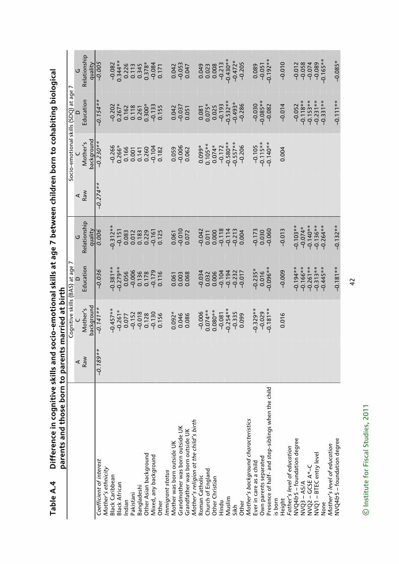
42
© In
stit
ute
for
Fisc
al S
tudi
es, 2
01
1
Tab
le A
.4
Dif
fere
nce
in c
og
nit
ive
skill
s an
d s
oci
o-e
mo
tio
nal
ski
lls a
t ag
e 7
bet
wee
n c
hild
ren
bo
rn t
o c
oh
abit
ing
bio
log
ical
p
aren
ts a
nd
th
ose
bo
rn t
o p
aren
ts m
arri
ed a
t b
irth
Cog
niti
ve s
kills
(B
AS)
at
age
7
Soci
o-em
otio
nal s
kills
(SD
Q) a
t ag
e 7
A
R
aw
C
Mot
her’
s ba
ckgr
ound
D
Edu
cati
on
G
Rel
atio
nshi
p qu
alit
y
A
Raw
C
M
othe
r’s
back
grou
nd
D
Edu
cati
on
G
Rel
atio
nshi
p qu
alit
y C
oeff
icie
nt o
f in
tere
st
–0.1
89
**
–0
.14
1*
*
–0.0
36
0
.00
6
–0.2
74
**
–0
.23
0*
*
–0.1
54
**
–0
.00
5
Mot
her’
s et
hnic
ity
Bla
ck C
arib
bean
–0.4
57*
*
–0.3
81*
*
–0.3
12*
*
–0
.266
–0
.202
–0
.082
B
lack
Afr
ican
–0.2
61*
–0
.279
**
–0
.151
0.26
6*
0.26
7*
0.34
4**
In
dian
0.07
7
0.05
6
0.08
3
0.
166
0.
162
0.
226
P
akis
tani
–0.1
52
–0.0
06
0.01
2
0.
001
0.
118
0.
113
B
angl
ades
hi
–0
.018
0.
136
0.
183
0.14
1
0.26
1
0.34
5
Oth
er A
sian
bac
kgro
und
0.
128
0.
178
0.
229
0.26
0
0.30
0*
0.37
8*
Mix
ed, a
ny b
ackg
roun
d
–0.1
30
–0.1
79
–0.1
61
–0
.104
–0
.133
–0
.084
O
ther
0.15
6
0.11
6
0.12
5
0.
182
0.
155
0.
171
Im
mig
rant
sta
tus
Mot
her
was
bor
n ou
tsid
e U
K
0.
092*
0.
061
0.
061
0.05
9
0.04
2
0.04
2
Gra
ndm
othe
r w
as b
orn
out
side
UK
0.04
6
0.00
3
–0.0
10
–0
.006
–0
.037
–0
.053
G
rand
fath
er w
as b
orn
outs
ide
UK
0.08
6
0.06
8
0.07
2
0.
062
0.
051
0.
047
M
othe
r’s
relig
ion
at
the
child
’s b
irth
R
oman
Cat
holic
–0.0
06
–0.0
34
–0.0
42
0.
099*
0.
081
0.
049
C
hurc
h o
f E
ngla
nd
0.
074*
*
0.03
2
0.01
1
0.
105*
*
0.07
5*
0.02
3
Oth
er C
hris
tian
0.08
0**
0.
006
0.
000
0.07
4*
0.02
5
0.00
8
Hin
du
–0
.081
–0
.104
–0
.118
–0.1
72
–0.1
93
–0.2
13
Mus
lim
–0
.254
**
–0
.194
–0
.114
–0.5
80*
*
–0.5
32*
*
–0.4
30*
*
Sikh
–0.3
35
–0.2
32
–0.2
13
–0
.557
**
–0
.493
*
–0.4
72*
O
ther
0.09
9
–0.0
17
0.00
4
–0
.206
–0
.286
–0
.205
M
othe
r’s
ba
ckg
roun
d c
hara
cter
isti
cs
Eve
r in
car
e as
a c
hild
–0.3
29*
*
–0.2
35*
–0
.173
–0.1
05
–0.0
30
0.08
9
Ow
n pa
rent
s se
para
ted
–0
.029
0.
016
0.
030
–0.1
15*
*
–0.0
85*
*
–0.0
51
Pre
senc
e of
hal
f- a
nd s
tep-
sibl
ings
whe
n th
e ch
ild
is b
orn
–0
.181
**
–0
.096
**
–0
.060
–0.1
40*
*
–0.0
82
–0.1
92*
*
Hei
ght
0.
016
–0
.009
–0
.013
0.00
4
–0.0
14
–0.0
10
Fa
ther
’s le
vel o
f ed
uca
tion
N
VQ
4&5
– fo
unda
tion
deg
ree
–0.1
94*
*
–0.1
03*
*
–0.0
52
–0.0
12
NV
Q3
– A
S/A
–0
.166
**
–0
.074
*
–0.1
18*
*
–0.0
58
NV
Q2
– G
CSE
A*–
C
–0.2
61*
*
–0.1
40*
*
–0.1
53*
*
–0.0
74
NV
Q1
– B
TEC
ent
ry le
vel
–0.3
13*
*
–0.1
36*
*
–0.2
31*
*
–0.0
89
Non
e
–0
.445
**
–0
.264
**
–0
.331
**
–0
.165
**
M
othe
r’s
leve
l of
educ
ati
on
NV
Q4&
5 –
foun
dati
on d
egre
e
–0
.181
**
–0
.132
**
–0
.111
**
–0
.085
*
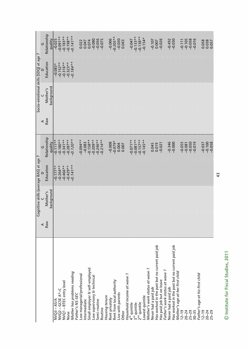
43
© In
stit
ute
for
Fisc
al S
tudi
es, 2
01
1
C
ogni
tive
ski
lls (
aver
age
BA
S) a
t ag
e 7
So
cio-
emot
iona
l ski
lls (S
DQ
) at
age
7
A
R
aw
C
Mot
her’
s ba
ckgr
ound
D
Edu
cati
on
G
Rel
atio
nshi
p qu
alit
y
A
Raw
C
M
othe
r’s
back
grou
nd
D
Edu
cati
on
G
Rel
atio
nshi
p qu
alit
y N
VQ
3 –
AS/
A
–0.1
77*
*
–0.1
11*
*
–0.0
83*
–0
.025
N
VQ
2 –
GC
SE A
*–C
–0
.264
**
–0
.180
**
–0
.152
**
–0
.091
**
N
VQ
1 –
BTE
C e
ntry
leve
l
–0
.466
**
–0
.341
**
–0
.316
**
–0
.183
**
N
one
–0.4
29*
*
–0.2
87*
*
–0.3
23*
*
–0.1
98*
*
Mot
her
has
prob
lem
s re
ad
ing
–0
.14
1*
*
–0.1
20
**
–0
.18
4*
*
–0.1
41
**
F
ath
er’s
NS-
SEC
Lo
w m
anag
eria
l/pr
ofes
sion
al
–0
.094
**
0.02
2
Inte
rmed
iate
–0.0
83
0.
047
Sm
all e
mpl
oyer
& s
elf-
empl
oyed
–0.1
58*
*
0.
074
Lo
w s
uper
viso
ry &
tec
hnic
al
–0
.209
**
–0.0
80
Sem
i-ro
utin
e
–0.2
46*
*
–0
.056
R
outi
ne
–0
.214
**
–0.0
75
Hou
sing
ten
ure
Ren
t pr
ivat
ely
–0
.008
–0.0
06
Ren
t fr
om lo
cal a
utho
rity
–0.0
79*
–0.2
05*
*
Live
wit
h pa
rent
s
0.00
4
–0
.020
O
ther
0.00
7
0.
043
H
ouse
hold
inco
me
at
wa
ve 1
4th
qui
ntile
–0.0
71*
*
–0
.047
3rd
qui
ntile
–0.0
81*
*
–0
.133
**
2nd
qui
ntile
–0.1
57*
*
–0
.138
**
Lo
wes
t qu
inti
le
–0
.145
**
–0.1
54*
M
othe
r’s
wor
k st
atu
s a
t w
ave
1
Nev
er h
ad a
pai
d jo
b
0.04
5
–0
.107
H
as w
orke
d in
the
pas
t bu
t no
cur
rent
pai
d jo
b
0.01
9
0.
007
H
as p
aid
job
but
on le
ave
–0
.021
–0.0
26
Fa
ther
’s w
ork
sta
tus
at
wa
ve 1
N
ever
had
a p
aid
job
–0
.346
–0.4
92
Has
wor
ked
in t
he p
ast
but
no c
urre
nt p
aid
job
–0
.000
–0.0
30
Mot
her’
s a
ge
at
her
firs
t ch
ild
12–1
9
–0
.055
–0.1
11
20–2
4
–0
.081
–0.1
05
25–2
9
–0
.050
–0.0
58
30–3
5
–0
.019
–0.0
16
Fa
ther
’s a
ge
at
his
firs
t ch
ild
12–1
9
–0
.037
0.05
8
20–2
4
–0
.100
0.03
8
25–2
9
–0
.058
0.05
7
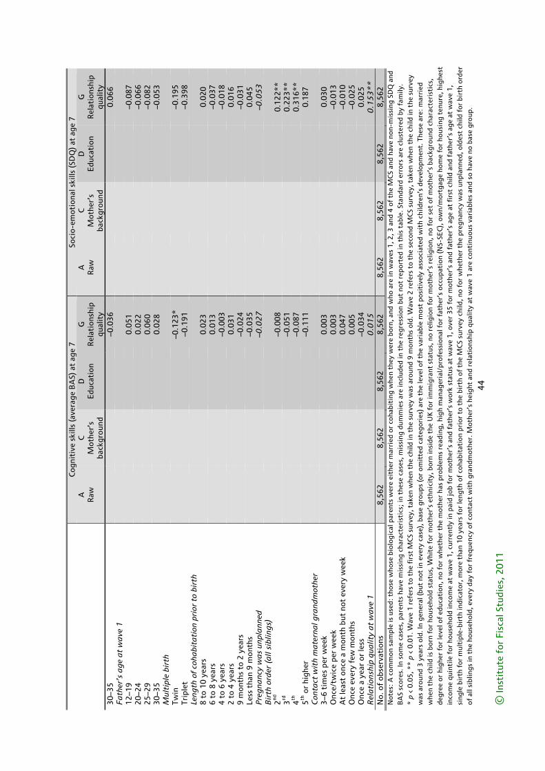
44
© In
stit
ute
for
Fisc
al S
tudi
es, 2
01
1
Not
es:
A c
omm
on
sam
ple
is u
sed
: th
ose
who
se b
iolo
gica
l par
ents
wer
e ei
ther
mar
ried
or
coha
biti
ng w
hen
they
wer
e bo
rn, a
nd w
ho a
re in
wav
es 1
, 2, 3
and
4 o
f th
e M
CS
and
have
non
-mis
sing
SD
Q a
nd
BA
S sc
ores
. In
som
e ca
ses,
par
ents
hav
e m
issi
ng c
hara
cter
isti
cs;
in t
hese
cas
es, m
issi
ng d
umm
ies
are
incl
uded
in t
he r
egre
ssio
n bu
t no
t re
port
ed in
thi
s ta
ble
. Sta
ndar
d e
rro
rs a
re c
lust
ered
by
fam
ily.
* p
< 0
.05
, **
p <
0.0
1. W
ave
1 r
efer
s to
the
fir
st M
CS
surv
ey, t
aken
whe
n th
e ch
ild in
the
sur
vey
was
aro
und
9 m
onth
s ol
d. W
ave
2 r
efer
s to
the
sec
ond
MC
S su
rvey
, tak
en w
hen
the
child
in t
he s
urve
y w
as a
roun
d 3
yea
rs o
ld. I
n ge
nera
l (bu
t no
t in
eve
ry c
ase)
, bas
e gr
oup
s (o
r om
itte
d c
ateg
orie
s) a
re t
he le
vel o
f th
e va
riab
le m
ost
posi
tive
ly a
ssoc
iate
d w
ith
child
ren’
s de
velo
pm
ent.
The
se a
re:
mar
ried
w
hen
the
child
is b
orn
for
hous
ehol
d st
atus
, Whi
te f
or
mot
her’
s et
hnic
ity,
bor
n in
side
the
UK
for
imm
igra
nt s
tatu
s, n
o re
ligio
n fo
r m
oth
er’s
rel
igio
n, n
o f
or
set
of
mot
her’
s ba
ckgr
ound
cha
ract
eris
tics
, de
gree
or
high
er f
or le
vel o
f ed
ucat
ion,
no
for
whe
ther
the
mot
her
has
prob
lem
s re
adin
g, h
igh
man
ager
ial/
pro
fess
iona
l fo
r fa
ther
’s o
ccup
atio
n (N
S-SE
C),
ow
n/m
ort
gage
ho
me
for
hous
ing
tenu
re, h
ighe
st
inco
me
quin
tile
fo
r ho
useh
old
inco
me
at w
ave
1, c
urre
ntly
in p
aid
job
for
mot
her’
s an
d fa
ther
’s w
ork
stat
us a
t w
ave
1, o
ver
35
for
mot
her’
s an
d fa
ther
’s a
ge a
t fi
rst
child
and
fat
her’
s ag
e at
wav
e 1,
si
ngle
bir
th f
or m
ulti
ple-
bir
th in
dica
tor,
mor
e th
an 1
0 y
ears
for
leng
th o
f co
habi
tati
on
pri
or t
o th
e bi
rth
of
the
MC
S su
rvey
chi
ld, n
o fo
r w
heth
er t
he p
reg
nanc
y w
as u
npla
nned
, old
est
child
for
bir
th o
rder
of
all
sibl
ings
in t
he h
ouse
hold
, eve
ry d
ay f
or f
requ
ency
of
cont
act
wit
h gr
and
mot
her.
Mot
her’
s he
ight
and
rel
atio
nshi
p qu
alit
y at
wav
e 1
are
con
tinu
ous
vari
able
s an
d so
hav
e no
bas
e gr
oup
.
C
ogni
tive
ski
lls (
aver
age
BA
S) a
t ag
e 7
So
cio-
emot
iona
l ski
lls (S
DQ
) at
age
7
A
R
aw
C
Mot
her’
s ba
ckgr
ound
D
Edu
cati
on
G
Rel
atio
nshi
p qu
alit
y
A
Raw
C
M
othe
r’s
back
grou
nd
D
Edu
cati
on
G
Rel
atio
nshi
p qu
alit
y 30
–35
–0.0
36
0.
066
F
ath
er’s
ag
e a
t w
ave
1
12–1
9
0.
051
–0.0
87
20–2
4
0.
022
–0.0
66
25–2
9
0.
060
–0.0
82
30–3
5
0.
028
–0.0
53
Mul
tipl
e b
irth
Tw
in
–0
.123
*
–0
.195
Tr
iple
t
–0.1
91
–0
.398
Le
ngth
of
coha
bit
ati
on p
rior
to
bir
th
8 t
o 1
0 y
ears
0.02
3
0.
020
6
to 8
yea
rs
0.
013
–0.0
37
4 to
6 y
ears
–0.0
03
–0
.018
2
to 4
yea
rs
0.
031
0.01
6
9 m
onth
s to
2 y
ears
–0.0
24
–0
.031
Le
ss t
han
9 m
ont
hs
–0
.035
0.04
5
Pre
gna
ncy
wa
s un
pla
nned
–0.0
27
–0.0
53
B
irth
ord
er (
all
sib
ling
s)
2nd
–0
.008
0.12
2**
3rd
–0.0
51
0.
223*
*
4th
–0
.087
0.31
6**
5th
or
high
er
–0
.111
0.18
7
Con
tact
wit
h m
ate
rna
l gra
ndm
othe
r
3–
6 ti
mes
per
wee
k
0.00
3
0.
030
O
nce/
twic
e pe
r w
eek
0.
003
–0.0
13
At
leas
t o
nce
a m
onth
but
not
eve
ry w
eek
0.
047
–0.0
10
Onc
e ev
ery
few
mon
ths
0.
005
–0.0
25
Onc
e a
year
or
less
–0.0
34
0.
025
R
ela
tion
ship
qua
lity
at
wa
ve 1
0.0
15
0.1
53
**
N
o. o
f ob
serv
atio
ns
8,56
2
8,56
2
8,56
2
8,56
2
8,56
2
8,56
2
8,56
2
8,56
2
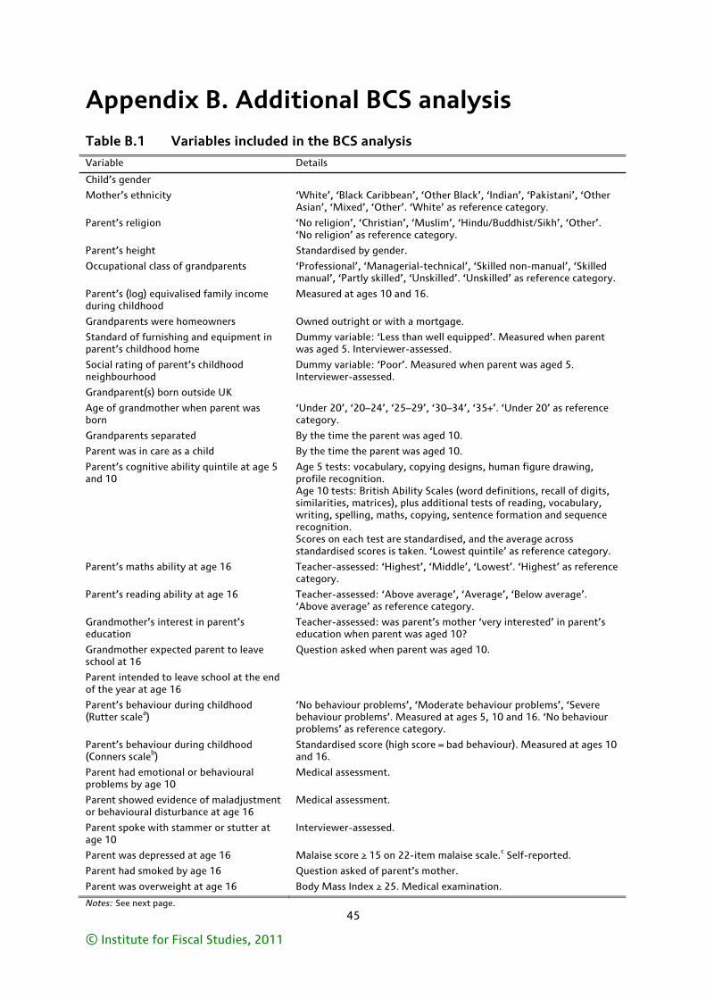
45
© Institute for Fiscal Studies, 2011
Appendix B. Additional BCS analysis
Table B.1 Variables included in the BCS analysis
Variable Details
Child’s gender
Mother’s ethnicity ‘White’, ‘Black Caribbean’, ‘Other Black’, ‘Indian’, ‘Pakistani’, ‘Other Asian’, ‘Mixed’, ‘Other’. ‘White’ as reference category.
Parent’s religion ‘No religion’, ‘Christian’, ‘Muslim’, ‘Hindu/Buddhist/Sikh’, ‘Other’. ‘No religion’ as reference category.
Parent’s height Standardised by gender.
Occupational class of grandparents ‘Professional’, ‘Managerial-technical’, ‘Skilled non-manual’, ‘Skilled manual’, ‘Partly skilled’, ‘Unskilled’. ‘Unskilled’ as reference category.
Parent’s (log) equivalised family income during childhood
Measured at ages 10 and 16.
Grandparents were homeowners Owned outright or with a mortgage.
Standard of furnishing and equipment in parent’s childhood home
Dummy variable: ‘Less than well equipped’. Measured when parent was aged 5. Interviewer-assessed.
Social rating of parent’s childhood neighbourhood
Dummy variable: ‘Poor’. Measured when parent was aged 5. Interviewer-assessed.
Grandparent(s) born outside UK
Age of grandmother when parent was born
‘Under 20’, ‘20–24’, ‘25–29’, ‘30–34’, ‘35+’. ‘Under 20’ as reference category.
Grandparents separated By the time the parent was aged 10.
Parent was in care as a child By the time the parent was aged 10.
Parent’s cognitive ability quintile at age 5 and 10
Age 5 tests: vocabulary, copying designs, human figure drawing, profile recognition. Age 10 tests: British Ability Scales (word definitions, recall of digits, similarities, matrices), plus additional tests of reading, vocabulary, writing, spelling, maths, copying, sentence formation and sequence recognition. Scores on each test are standardised, and the average across standardised scores is taken. ‘Lowest quintile’ as reference category.
Parent’s maths ability at age 16 Teacher-assessed: ‘Highest’, ‘Middle’, ‘Lowest’. ‘Highest’ as reference category.
Parent’s reading ability at age 16 Teacher-assessed: ‘Above average’, ‘Average’, ‘Below average’. ‘Above average’ as reference category.
Grandmother’s interest in parent’s education
Teacher-assessed: was parent’s mother ‘very interested’ in parent’s education when parent was aged 10?
Grandmother expected parent to leave school at 16
Question asked when parent was aged 10.
Parent intended to leave school at the end of the year at age 16
Parent’s behaviour during childhood (Rutter scalea)
‘No behaviour problems’, ‘Moderate behaviour problems’, ‘Severe behaviour problems’. Measured at ages 5, 10 and 16. ‘No behaviour problems’ as reference category.
Parent’s behaviour during childhood (Conners scaleb)
Standardised score (high score = bad behaviour). Measured at ages 10 and 16.
Parent had emotional or behavioural problems by age 10
Medical assessment.
Parent showed evidence of maladjustment or behavioural disturbance at age 16
Medical assessment.
Parent spoke with stammer or stutter at age 10
Interviewer-assessed.
Parent was depressed at age 16 Malaise score ≥ 15 on 22-item malaise scale.c Self-reported.
Parent had smoked by age 16 Question asked of parent’s mother.
Parent was overweight at age 16 Body Mass Index ≥ 25. Medical examination.
Notes: See next page.
Cohabitation, marriage, relationship stability and child outcomes: an update
46
© Institute for Fiscal Studies, 2011
Notes to Table B.1 a. See http://www.cls.ioe.ac.uk/core/documents/download.asp?id=932&log_stat=1 for details. b. See Conners (1969) for details. c. See http://www.cls.ioe.ac.uk/core/documents/download.asp?id=938&log_stat=1 for details. Notes: The ‘parent’ here refers to the cohort member of the BCS, for whom we observe a rich set of information from their own childhood. The other parent of the children in our sample is not a cohort member of the BCS, and hence we do not observe such information about them.
Table B.2 shows the results from the same regression analysis as in Chapter 4 conducted on each individual subscale of the BAS and SDQ cognitive and socio-emotional measures. Since only children of particular ages took individual BAS tests, the results shown are unlikely to be representative, because children’s age in the BCS is collinear with the age of one of their parents at birth (see Chapter 2 for further discussion of these issues).
Table B.2 Difference in cognitive and socio-emotional development between children born to cohabiting and married parents: individual BAS and SDQ scales
Explanatory variables (besides marital status of parents at child’s birth)
(1) None
(2) Predetermined characteristics
available in MCS
(3) Additional
predetermined characteristics
available in BCS Outcome variable (sample size in parentheses) BAS naming vocabulary, ages 3 to 5 (1,118) –0.026 –0.018 0.057 BAS early number concepts, ages 3 to 5 (1,108) –0.131 –0.122 –0.046 BAS word reading, ages 6 to 16 (1,902) –0.214** –0.208** –0.075 BAS number skills, ages 6 to 16 (1,896) –0.180** –0.165** –0.048 SDQ emotional score, ages 5 to 15 (2,291) –0.067 –0.076 –0.010 SDQ conduct score, ages 5 to 15 (2,291) –0.243** –0.220** –0.108* SDQ hyperactivity score, ages 5 to 15 (2,293) –0.094* –0.079 –0.009 SDQ peer relationship score, ages 5 to 15 (2,293) –0.129** –0.132** –0.042 Notes: Numbers are regression coefficients on a dummy variable ‘parents were cohabiting at the time of the child’s birth’; the omitted category is therefore children whose parents were married at the time of their birth. Sets of control variables are identical to those in the main analysis: see Table 4.2. All other coefficient estimates are available from the authors on request. Standard errors are clustered by family. * p < 0.05, ** p < 0.01.
Decomposition analysis
A decomposition analysis can be used to split the raw gap in outcomes between children born to married and cohabiting parents into various components, corresponding to that part of the gap which is explained by particular observable factors. Take parental cognitive ability as an example. The extent to which parental cognitive ability is an important source of selection into marriage depends upon two things:
1. the extent to which parental cognitive ability differs between children born to cohabiting and married parents (this is directly observable in our sample);
2. the size of the impact of parental cognitive ability on the child outcomes that we are investigating (which we have estimated in the regression models shown in column 3 of Table 4.2).
For every variable included in our model, we can therefore calculate its contribution to the ‘raw’ gap in outcomes between children born to married and cohabiting parents. This contribution is equal to the difference between the average values of that variable for children born to married and cohabiting parents, multiplied by its coefficient estimate from the regression. Two things should thus be borne in mind when interpreting these results. First, the contributions are calculated taking all other observable characteristics into account. For example, a significant contribution of parental cognitive ability to the gap
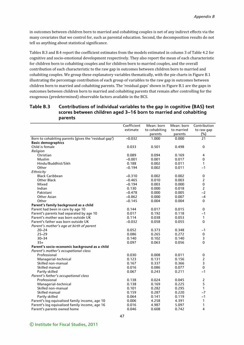
Appendix B
47
© Institute for Fiscal Studies, 2011
in outcomes between children born to married and cohabiting couples is net of any indirect effects via the many covariates that we control for, such as parental education. Second, the decomposition results do not tell us anything about statistical significance.
Tables B.3 and B.4 report the coefficient estimates from the models estimated in column 3 of Table 4.2 for cognitive and socio-emotional development respectively. They also report the mean of each characteristic for children born to cohabiting couples and for children born to married couples, and the overall contribution of each characteristic to the raw gap in outcomes between children born to married and cohabiting couples. We group these explanatory variables thematically, with the pie charts in Figure B.1 illustrating the percentage contribution of each group of variables to the raw gap in outcomes between children born to married and cohabiting parents. The ‘residual gaps’ shown in Figure B.1 are the gaps in outcomes between children born to married and cohabiting parents that remain after controlling for the exogenous (predetermined) observable factors available in the BCS.
Table B.3 Contributions of individual variables to the gap in cognitive (BAS) test scores between children aged 3–16 born to married and cohabiting parents
Coefficient estimate
Mean: born to cohabiting
parents
Mean: born to married
parents
Contribution to raw gap
(%) Born to cohabiting parents (gives the ‘residual gap’) –0.032 1.000 0.000 21 Basic demographics Child is female 0.033 0.501 0.498 0 Religion Christian 0.089 0.094 0.169 4 Muslim –0.001 0.001 0.017 0 Hindu/Buddhist/Sikh 0.188 0.002 0.011 1 Other –0.194 0.002 0.011 –1 Ethnicity Black Caribbean –0.310 0.002 0.002 0 Other Black –0.465 0.010 0.003 2 Mixed –0.194 0.003 0.000 0 Indian 0.130 0.000 0.018 2 Pakistani –0.478 0.000 0.005 –2 Other Asian –0.862 0.000 0.007 –4 Other –0.145 0.004 0.004 0 Parent’s family background as a child Parent had been in care by age 10 0.144 0.017 0.015 0 Parent’s parents had separated by age 10 0.017 0.192 0.118 –1 Parent’s mother was born outside UK 0.114 0.038 0.053 1 Parent’s father was born outside UK –0.032 0.058 0.055 0 Parent’s mother’s age at birth of parent 20–24 0.052 0.373 0.348 –1 25–29 0.086 0.265 0.272 0 30–34 0.140 0.102 0.140 3 35+ 0.097 0.063 0.056 0 Parent’s socio-economic background as a child Parent’s mother’s occupational class Professional 0.030 0.008 0.011 0 Managerial-technical 0.123 0.131 0.156 2 Skilled non-manual 0.167 0.337 0.366 3 Skilled manual 0.016 0.086 0.077 0 Partly skilled 0.067 0.243 0.211 –1 Parent’s father’s occupational class Professional 0.138 0.024 0.045 2 Managerial-technical 0.138 0.169 0.225 5 Skilled non-manual 0.101 0.282 0.295 1 Skilled manual 0.159 0.287 0.220 –7 Partly skilled 0.064 0.141 0.119 –1 Parent’s log equivalised family income, age 10 0.006 4.258 4.391 1 Parent’s log equivalised family income, age 16 0.016 4.987 5.097 1 Parent’s parents owned home 0.046 0.608 0.742 4
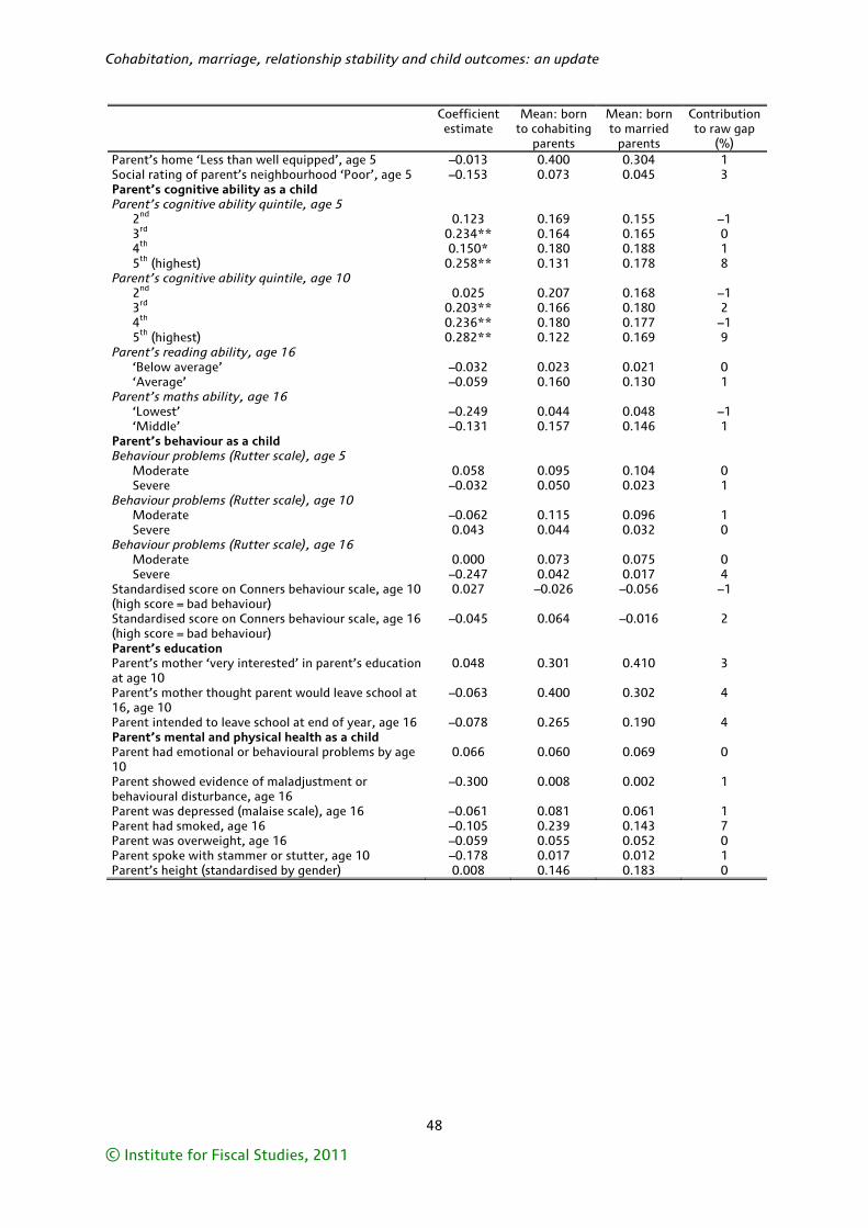
Cohabitation, marriage, relationship stability and child outcomes: an update
48
© Institute for Fiscal Studies, 2011
Coefficient estimate
Mean: born to cohabiting
parents
Mean: born to married
parents
Contribution to raw gap
(%) Parent’s home ‘Less than well equipped’, age 5 –0.013 0.400 0.304 1 Social rating of parent’s neighbourhood ‘Poor’, age 5 –0.153 0.073 0.045 3 Parent’s cognitive ability as a child Parent’s cognitive ability quintile, age 5 2nd 0.123 0.169 0.155 –1 3rd 0.234** 0.164 0.165 0 4th 0.150* 0.180 0.188 1 5th (highest) 0.258** 0.131 0.178 8 Parent’s cognitive ability quintile, age 10 2nd 0.025 0.207 0.168 –1 3rd 0.203** 0.166 0.180 2 4th 0.236** 0.180 0.177 –1 5th (highest) 0.282** 0.122 0.169 9 Parent’s reading ability, age 16 ‘Below average’ –0.032 0.023 0.021 0 ‘Average’ –0.059 0.160 0.130 1 Parent’s maths ability, age 16 ‘Lowest’ –0.249 0.044 0.048 –1 ‘Middle’ –0.131 0.157 0.146 1 Parent’s behaviour as a child Behaviour problems (Rutter scale), age 5 Moderate 0.058 0.095 0.104 0 Severe –0.032 0.050 0.023 1 Behaviour problems (Rutter scale), age 10 Moderate –0.062 0.115 0.096 1 Severe 0.043 0.044 0.032 0 Behaviour problems (Rutter scale), age 16 Moderate 0.000 0.073 0.075 0 Severe –0.247 0.042 0.017 4 Standardised score on Conners behaviour scale, age 10 (high score = bad behaviour)
0.027 –0.026 –0.056 –1
Standardised score on Conners behaviour scale, age 16 (high score = bad behaviour)
–0.045 0.064 –0.016 2
Parent’s education Parent’s mother ‘very interested’ in parent’s education at age 10
0.048 0.301 0.410 3
Parent’s mother thought parent would leave school at 16, age 10
–0.063 0.400 0.302 4
Parent intended to leave school at end of year, age 16 –0.078 0.265 0.190 4 Parent’s mental and physical health as a child Parent had emotional or behavioural problems by age 10
0.066 0.060 0.069 0
Parent showed evidence of maladjustment or behavioural disturbance, age 16
–0.300 0.008 0.002 1
Parent was depressed (malaise scale), age 16 –0.061 0.081 0.061 1 Parent had smoked, age 16 –0.105 0.239 0.143 7 Parent was overweight, age 16 –0.059 0.055 0.052 0 Parent spoke with stammer or stutter, age 10 –0.178 0.017 0.012 1 Parent’s height (standardised by gender) 0.008 0.146 0.183 0
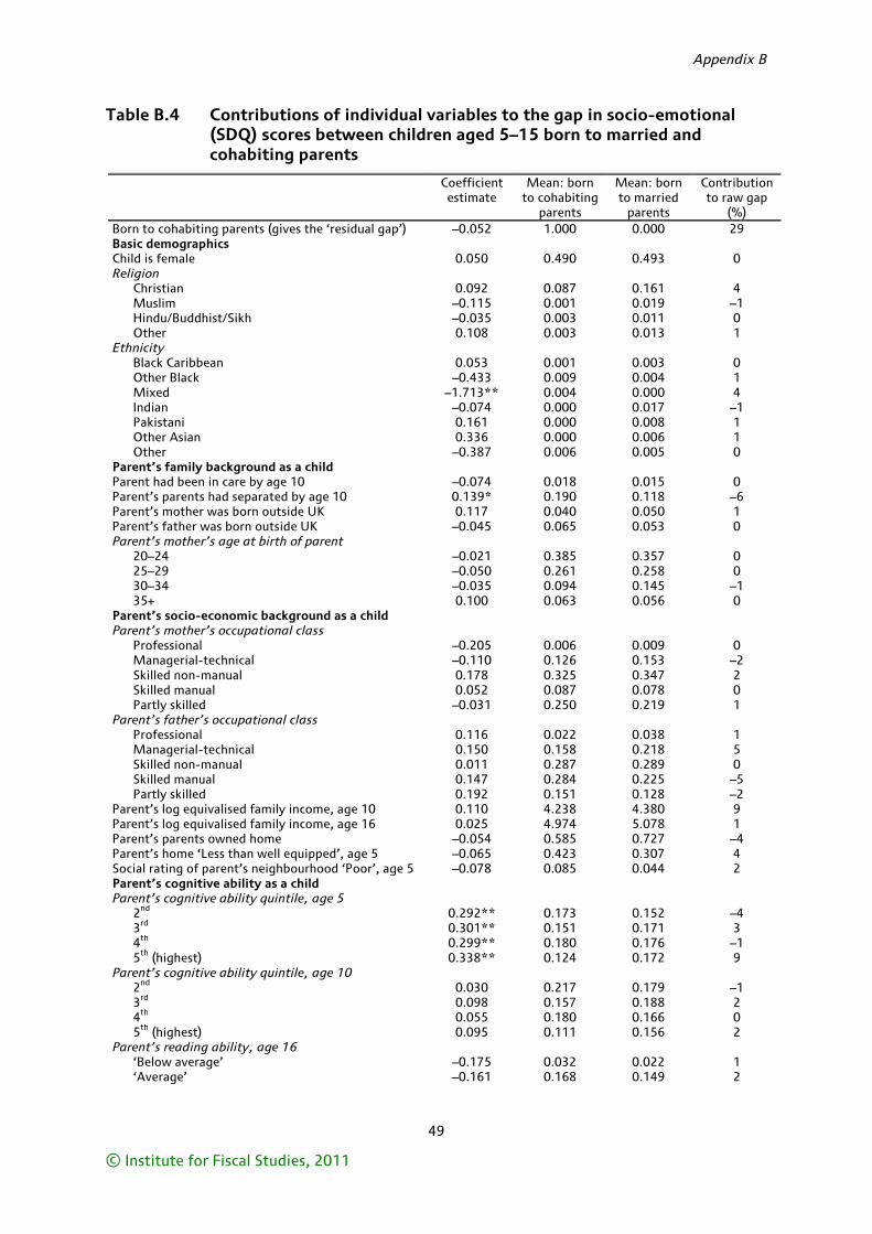
Appendix B
49
© Institute for Fiscal Studies, 2011
Table B.4 Contributions of individual variables to the gap in socio-emotional (SDQ) scores between children aged 5–15 born to married and cohabiting parents
Coefficient estimate
Mean: born to cohabiting
parents
Mean: born to married
parents
Contribution to raw gap
(%) Born to cohabiting parents (gives the ‘residual gap’) –0.052 1.000 0.000 29 Basic demographics Child is female 0.050 0.490 0.493 0 Religion Christian 0.092 0.087 0.161 4 Muslim –0.115 0.001 0.019 –1 Hindu/Buddhist/Sikh –0.035 0.003 0.011 0 Other 0.108 0.003 0.013 1 Ethnicity Black Caribbean 0.053 0.001 0.003 0 Other Black –0.433 0.009 0.004 1 Mixed –1.713** 0.004 0.000 4 Indian –0.074 0.000 0.017 –1 Pakistani 0.161 0.000 0.008 1 Other Asian 0.336 0.000 0.006 1 Other –0.387 0.006 0.005 0 Parent’s family background as a child Parent had been in care by age 10 –0.074 0.018 0.015 0 Parent’s parents had separated by age 10 0.139* 0.190 0.118 –6 Parent’s mother was born outside UK 0.117 0.040 0.050 1 Parent’s father was born outside UK –0.045 0.065 0.053 0 Parent’s mother’s age at birth of parent 20–24 –0.021 0.385 0.357 0 25–29 –0.050 0.261 0.258 0 30–34 –0.035 0.094 0.145 –1 35+ 0.100 0.063 0.056 0 Parent’s socio-economic background as a child Parent’s mother’s occupational class Professional –0.205 0.006 0.009 0 Managerial-technical –0.110 0.126 0.153 –2 Skilled non-manual 0.178 0.325 0.347 2 Skilled manual 0.052 0.087 0.078 0 Partly skilled –0.031 0.250 0.219 1 Parent’s father’s occupational class Professional 0.116 0.022 0.038 1 Managerial-technical 0.150 0.158 0.218 5 Skilled non-manual 0.011 0.287 0.289 0 Skilled manual 0.147 0.284 0.225 –5 Partly skilled 0.192 0.151 0.128 –2 Parent’s log equivalised family income, age 10 0.110 4.238 4.380 9 Parent’s log equivalised family income, age 16 0.025 4.974 5.078 1 Parent’s parents owned home –0.054 0.585 0.727 –4 Parent’s home ‘Less than well equipped’, age 5 –0.065 0.423 0.307 4 Social rating of parent’s neighbourhood ‘Poor’, age 5 –0.078 0.085 0.044 2 Parent’s cognitive ability as a child Parent’s cognitive ability quintile, age 5 2nd 0.292** 0.173 0.152 –4 3rd 0.301** 0.151 0.171 3 4th 0.299** 0.180 0.176 –1 5th (highest) 0.338** 0.124 0.172 9 Parent’s cognitive ability quintile, age 10 2nd 0.030 0.217 0.179 –1 3rd 0.098 0.157 0.188 2 4th 0.055 0.180 0.166 0 5th (highest) 0.095 0.111 0.156 2 Parent’s reading ability, age 16 ‘Below average’ –0.175 0.032 0.022 1 ‘Average’ –0.161 0.168 0.149 2
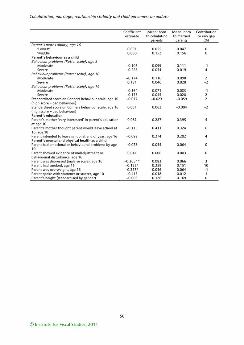
Cohabitation, marriage, relationship stability and child outcomes: an update
50
© Institute for Fiscal Studies, 2011
Coefficient estimate
Mean: born to cohabiting
parents
Mean: born to married
parents
Contribution to raw gap
(%) Parent’s maths ability, age 16 ‘Lowest’ 0.091 0.055 0.047 0 ‘Middle’ 0.030 0.152 0.156 0 Parent’s behaviour as a child Behaviour problems (Rutter scale), age 5 Moderate –0.106 0.099 0.111 –1 Severe –0.228 0.054 0.019 4 Behaviour problems (Rutter scale), age 10 Moderate –0.174 0.116 0.098 2 Severe 0.181 0.046 0.028 –2 Behaviour problems (Rutter scale), age 16 Moderate –0.164 0.071 0.083 –1 Severe –0.173 0.045 0.020 2 Standardised score on Conners behaviour scale, age 10 (high score = bad behaviour)
–0.077 –0.023 –0.059 2
Standardised score on Conners behaviour scale, age 16 (high score = bad behaviour)
0.051 0.062 –0.004 –2
Parent’s education Parent’s mother ‘very interested’ in parent’s education at age 10
0.087 0.287 0.395 5
Parent’s mother thought parent would leave school at 16, age 10
–0.113 0.411 0.324 6
Parent intended to leave school at end of year, age 16 –0.093 0.274 0.202 4 Parent’s mental and physical health as a child Parent had emotional or behavioural problems by age 10
–0.078 0.055 0.064 0
Parent showed evidence of maladjustment or behavioural disturbance, age 16
0.041 0.006 0.003 0
Parent was depressed (malaise scale), age 16 –0.365** 0.083 0.066 3 Parent had smoked, age 16 –0.155* 0.259 0.151 10 Parent was overweight, age 16 –0.227* 0.056 0.064 –1 Parent spoke with stammer or stutter, age 10 –0.415 0.018 0.012 1 Parent’s height (standardised by gender) –0.005 0.126 0.169 0
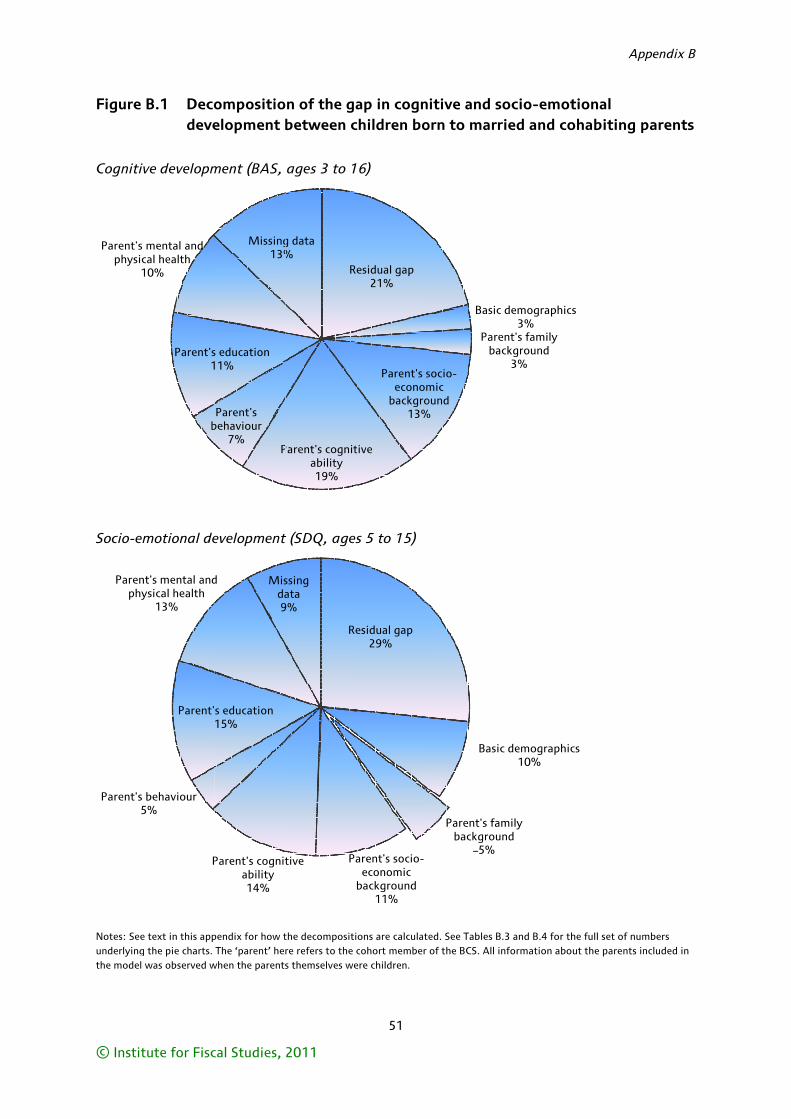
© Instit
Figure
Cogniti
Socio-em
Notes: Seeunderlyingthe model
Parent's physic
1
Parent's 5
Parenphy
tute for Fisc
B.1 Decodeve
ve developm
motional de
e text in this appg the pie charts.
was observed w
b
Parent's1
mental and cal health10%
P
behaviour5%
Parent'
nt's mental andysical health
13%
cal Studies,
ompositioelopment b
ment (BAS,
evelopment
pendix for how tThe ‘parent’ her
when the parents
P
Parent's behaviour
7%
s education11%
Missing13%
Parent's cognitability14%
s education15%
d Misda9
2011
n of the gabetween c
ages 3 to 1
t (SDQ, ages
the decompositire refers to the cs themselves we
Re
Parent's cognitability19%
g data%
Re
Pa
b
tive
ssing ata
9%
51
ap in cognhildren bo
6)
s 5 to 15)
ons are calculatecohort member ere children.
esidual gap21%
Parent's seconom
backgro13%
ive
esidual gap29%
arent's socio-economic
background11%
itive and sorn to marr
ed. See Tables Bof the BCS. All i
Basic
Pareba
socio-mic ound%
Basic
Parent's fabackgrou
–5%
socio-emotried and co
B.3 and B.4 for thnformation abo
c demographic3%
ent's family ckground
3%
c demographic10%
mily nd
Ap
tional ohabiting p
he full set of numut the parents in
s
cs
ppendix B
parents
mbers ncluded in
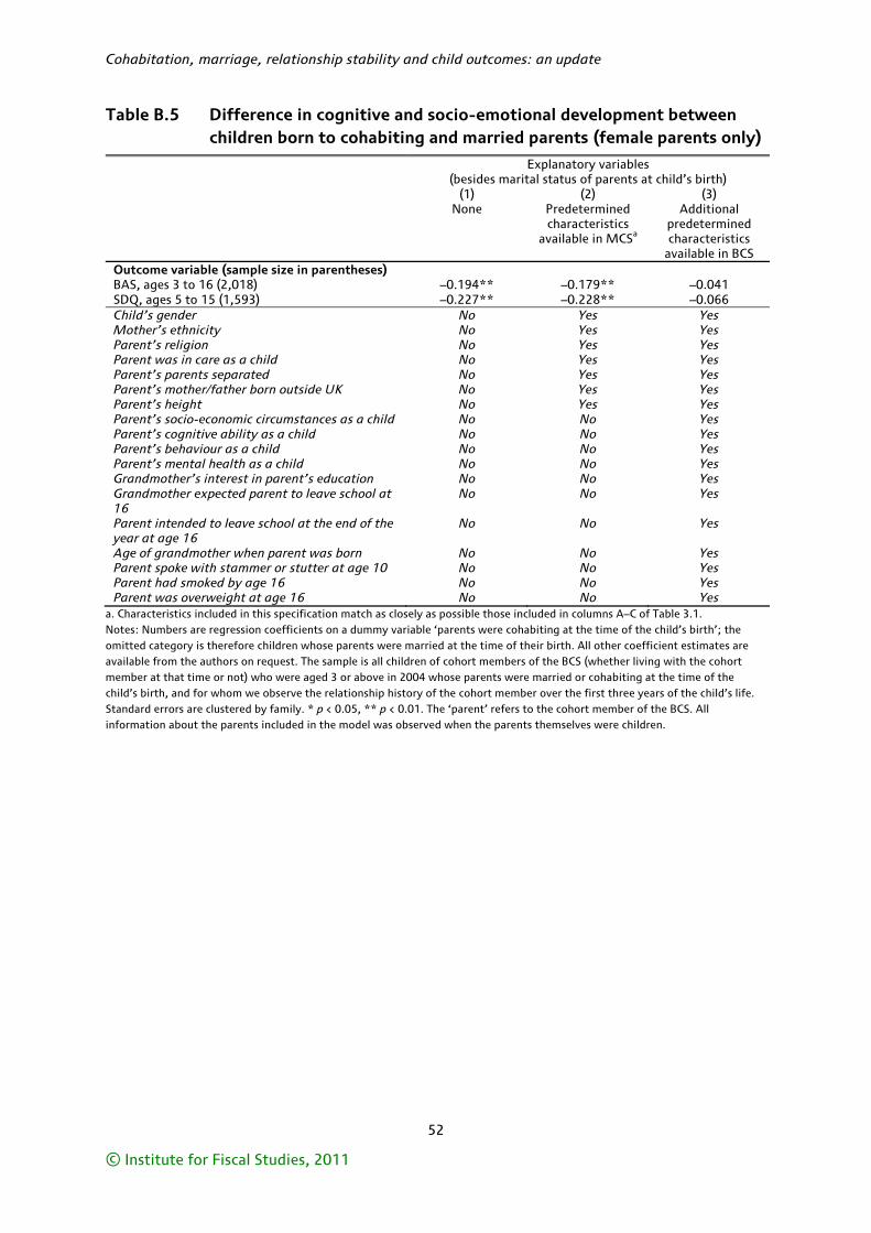
Cohabitation, marriage, relationship stability and child outcomes: an update
52
© Institute for Fiscal Studies, 2011
Table B.5 Difference in cognitive and socio-emotional development between children born to cohabiting and married parents (female parents only)
Explanatory variables (besides marital status of parents at child’s birth)
(1) None
(2) Predetermined characteristics
available in MCSa
(3) Additional
predetermined characteristics
available in BCS Outcome variable (sample size in parentheses) BAS, ages 3 to 16 (2,018) –0.194** –0.179** –0.041 SDQ, ages 5 to 15 (1,593) –0.227** –0.228** –0.066 Child’s gender No Yes Yes Mother’s ethnicity No Yes Yes Parent’s religion No Yes Yes Parent was in care as a child No Yes Yes Parent’s parents separated No Yes Yes Parent’s mother/father born outside UK No Yes Yes Parent’s height No Yes Yes Parent’s socio-economic circumstances as a child No No Yes Parent’s cognitive ability as a child No No Yes Parent’s behaviour as a child No No Yes Parent’s mental health as a child No No Yes Grandmother’s interest in parent’s education No No Yes Grandmother expected parent to leave school at 16
No No Yes
Parent intended to leave school at the end of the year at age 16
No No Yes
Age of grandmother when parent was born No No Yes Parent spoke with stammer or stutter at age 10 No No Yes Parent had smoked by age 16 No No Yes Parent was overweight at age 16 No No Yes
a. Characteristics included in this specification match as closely as possible those included in columns A–C of Table 3.1. Notes: Numbers are regression coefficients on a dummy variable ‘parents were cohabiting at the time of the child’s birth’; the omitted category is therefore children whose parents were married at the time of their birth. All other coefficient estimates are available from the authors on request. The sample is all children of cohort members of the BCS (whether living with the cohort member at that time or not) who were aged 3 or above in 2004 whose parents were married or cohabiting at the time of the child’s birth, and for whom we observe the relationship history of the cohort member over the first three years of the child’s life. Standard errors are clustered by family. * p < 0.05, ** p < 0.01. The ‘parent’ refers to the cohort member of the BCS. All information about the parents included in the model was observed when the parents themselves were children.
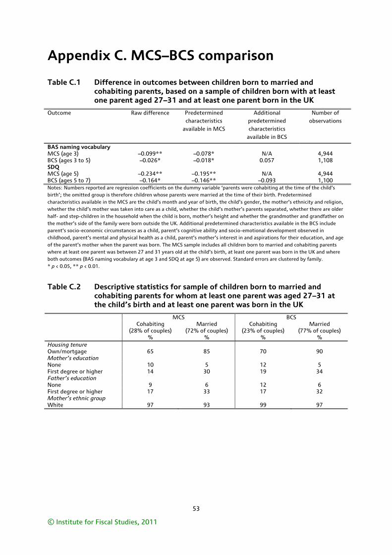
53
© Institute for Fiscal Studies, 2011
Appendix C. MCS–BCS comparison
Table C.1 Difference in outcomes between children born to married and cohabiting parents, based on a sample of children born with at least one parent aged 27–31 and at least one parent born in the UK
Outcome Raw difference Predetermined characteristics
available in MCS
Additional predetermined characteristics
available in BCS
Number of observations
BAS naming vocabulary MCS (age 3) –0.099** –0.078* N/A 4,944 BCS (ages 3 to 5) –0.026* –0.018* 0.057 1,108 SDQ MCS (age 5) –0.234** –0.195** N/A 4,944 BCS (ages 5 to 7) –0.164* –0.146** –0.093 1,100 Notes: Numbers reported are regression coefficients on the dummy variable ‘parents were cohabiting at the time of the child’s birth’; the omitted group is therefore children whose parents were married at the time of their birth. Predetermined characteristics available in the MCS are the child’s month and year of birth, the child’s gender, the mother’s ethnicity and religion, whether the child’s mother was taken into care as a child, whether the child’s mother’s parents separated, whether there are older half- and step-children in the household when the child is born, mother’s height and whether the grandmother and grandfather on the mother’s side of the family were born outside the UK. Additional predetermined characteristics available in the BCS include parent’s socio-economic circumstances as a child, parent’s cognitive ability and socio-emotional development observed in childhood, parent’s mental and physical health as a child, parent’s mother’s interest in and aspirations for their education, and age of the parent’s mother when the parent was born. The MCS sample includes all children born to married and cohabiting parents where at least one parent was between 27 and 31 years old at the child’s birth, at least one parent was born in the UK and where both outcomes (BAS naming vocabulary at age 3 and SDQ at age 5) are observed. Standard errors are clustered by family. * p < 0.05, ** p < 0.01.
Table C.2 Descriptive statistics for sample of children born to married and cohabiting parents for whom at least one parent was aged 27–31 at the child’s birth and at least one parent was born in the UK
MCS BCS Cohabiting
(28% of couples) %
Married (72% of couples)
%
Cohabiting (23% of couples)
%
Married (77% of couples)
% Housing tenure Own/mortgage 65 85 70 90 Mother’s education None 10 5 12 5 First degree or higher 14 30 19 34 Father’s education None 9 6 12 6 First degree or higher 17 33 17 32 Mother’s ethnic group White 97 93 99 97
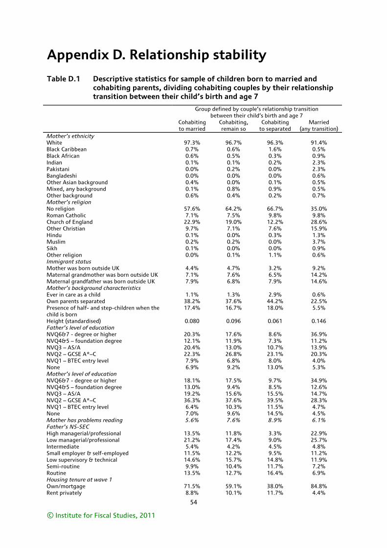
54
© Institute for Fiscal Studies, 2011
Appendix D. Relationship stability
Table D.1 Descriptive statistics for sample of children born to married and cohabiting parents, dividing cohabiting couples by their relationship transition between their child’s birth and age 7
Group defined by couple’s relationship transition between their child’s birth and age 7
Cohabiting to married
Cohabiting, remain so
Cohabiting to separated
Married (any transition)
Mother’s ethnicity White 97.3% 96.7% 96.3% 91.4% Black Caribbean 0.7% 0.6% 1.6% 0.5% Black African 0.6% 0.5% 0.3% 0.9% Indian 0.1% 0.1% 0.2% 2.3% Pakistani 0.0% 0.2% 0.0% 2.3% Bangladeshi 0.0% 0.0% 0.0% 0.6% Other Asian background 0.4% 0.0% 0.1% 0.5% Mixed, any background 0.1% 0.8% 0.9% 0.5% Other background 0.6% 0.4% 0.2% 0.7% Mother’s religion No religion 57.6% 64.2% 66.7% 35.0% Roman Catholic 7.1% 7.5% 9.8% 9.8% Church of England 22.9% 19.0% 12.2% 28.6% Other Christian 9.7% 7.1% 7.6% 15.9% Hindu 0.1% 0.0% 0.3% 1.3% Muslim 0.2% 0.2% 0.0% 3.7% Sikh 0.1% 0.0% 0.0% 0.9% Other religion 0.0% 0.1% 1.1% 0.6% Immigrant status Mother was born outside UK 4.4% 4.7% 3.2% 9.2% Maternal grandmother was born outside UK 7.1% 7.6% 6.5% 14.2% Maternal grandfather was born outside UK 7.9% 6.8% 7.9% 14.6% Mother’s background characteristics Ever in care as a child 1.1% 1.3% 2.9% 0.6% Own parents separated 38.2% 37.6% 44.2% 22.5% Presence of half- and step-children when the child is born
17.4% 16.7% 18.0% 5.5%
Height (standardised) 0.080 0.096 0.061 0.146 Father’s level of education NVQ6&7 - degree or higher 20.3% 17.6% 8.6% 36.9% NVQ4&5 – foundation degree 12.1% 11.9% 7.3% 11.2% NVQ3 – AS/A 20.4% 13.0% 10.7% 13.9% NVQ2 – GCSE A*–C 22.3% 26.8% 23.1% 20.3% NVQ1 – BTEC entry level 7.9% 6.8% 8.0% 4.0% None 6.9% 9.2% 13.0% 5.3% Mother’s level of education NVQ6&7 - degree or higher 18.1% 17.5% 9.7% 34.9% NVQ4&5 – foundation degree 13.0% 9.4% 8.5% 12.6% NVQ3 – AS/A 19.2% 15.6% 15.5% 14.7% NVQ2 – GCSE A*–C 36.3% 37.6% 39.5% 28.3% NVQ1 – BTEC entry level 6.4% 10.3% 11.5% 4.7% None 7.0% 9.6% 14.5% 4.5% Mother has problems reading 5.6% 7.6% 8.9% 6.1% Father’s NS-SEC High managerial/professional 13.5% 11.8% 3.3% 22.9% Low managerial/professional 21.2% 17.4% 9.0% 25.7% Intermediate 5.4% 4.2% 4.5% 4.8% Small employer & self-employed 11.5% 12.2% 9.5% 11.2% Low supervisory & technical 14.6% 15.7% 14.8% 11.9% Semi-routine 9.9% 10.4% 11.7% 7.2% Routine 13.5% 12.7% 16.4% 6.9% Housing tenure at wave 1 Own/mortgage 71.5% 59.1% 38.0% 84.8% Rent privately 8.8% 10.1% 11.7% 4.4%
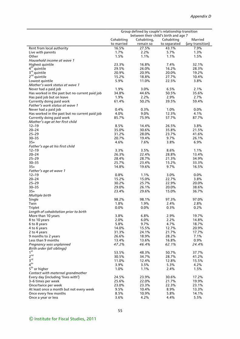
Appendix D
55
© Institute for Fiscal Studies, 2011
Group defined by couple’s relationship transition between their child’s birth and age 7
Cohabiting to married
Cohabiting, remain so
Cohabiting to separated
Married (any transition)
Rent from local authority 16.5% 27.5% 43.1% 7.9% Live with parents 1.7% 2.2% 5.7% 1.3% Other 1.5% 1.1% 1.1% 1.5% Household income at wave 1 Highest quintile 23.3% 16.8% 7.4% 32.1% 4th quintile 29.5% 26.0% 16.2% 28.3% 3rd quintile 20.9% 20.9% 20.0% 19.2% 2nd quintile 15.2% 18.8% 27.7% 10.4% Lowest quintile 5.9% 11.0% 22.5% 3.8% Mother’s work status at wave 1 Never had a paid job 1.9% 3.0% 6.5% 2.1% Has worked in the past but no current paid job 34.8% 44.6% 50.5% 35.6% Has paid job but on leave 1.9% 2.2% 2.9% 2.7% Currently doing paid work 61.4% 50.2% 39.5% 59.4% Father’s work status at wave 1 Never had a paid job 0.4% 0.3% 1.0% 0.0% Has worked in the past but no current paid job 4.0% 9.0% 12.3% 4.1% Currently doing paid work 85.7% 75.9% 57.7% 87.7% Mother’s age at her first child 12–19 8.5% 14.4% 26.5% 3.8% 20–24 35.0% 30.6% 35.8% 21.5% 25–29 31.2% 28.0% 23.7% 41.6% 30–35 20.7% 19.4% 9.7% 26.1% 35+ 4.6% 7.6% 3.8% 6.9% Father’s age at his first child 12–19 3.3% 3.5% 8.6% 1.1% 20–24 26.3% 22.4% 28.8% 13.4% 25–29 28.4% 28.7% 21.3% 34.9% 30–35 25.7% 23.4% 15.2% 33.3% 35+ 14.8% 19.6% 9.7% 16.5% Father’s age at wave 1 12–19 0.8% 1.1% 3.0% 0.0% 20–24 15.2% 15.0% 22.7% 3.8% 25–29 30.2% 25.7% 22.9% 20.0% 30–35 29.0% 26.1% 20.0% 38.6% 35+ 23.4% 29.6% 15.0% 36.7% Multiple birth Single 98.2% 98.1% 97.3% 97.0% Twin 1.8% 1.9% 2.4% 2.8% Triplet 0.0% 0.0% 0.3% 0.2% Length of cohabitation prior to birth More than 10 years 3.8% 6.8% 2.9% 19.7% 8 to 10 years 2.0% 6.0% 2.2% 14.8% 6 to 8 years 5.8% 9.7% 4.7% 18.7% 4 to 6 years 14.0% 15.5% 12.7% 20.9% 2 to 4 years 31.3% 24.1% 21.7% 17.7% 9 months to 2 years 26.6% 18.9% 28.2% 7.1% Less than 9 months 13.4% 13.6% 16.8% 0.9% Pregnancy was unplanned 47.2% 46.4% 62.1% 24.4% Birth order (all siblings) 1st 53.5% 48.3% 50.7% 37.7% 2nd 30.5% 34.7% 28.7% 41.2% 3rd 11.0% 12.4% 12.8% 15.5% 4th 3.9% 3.5% 5.3% 4.2% 5th or higher 1.0% 1.1% 2.4% 1.5% Contact with maternal grandmother Every day (including ‘lives with’) 24.5% 23.9% 30.6% 17.2% 3–6 times per week 25.6% 22.0% 21.7% 19.9% Once/twice per week 23.0% 23.3% 22.3% 23.1% At least once a month but not every week 9.5% 10.4% 8.9% 13.3% Once every few months 8.5% 10.9% 5.8% 14.1% Once a year or less 3.6% 4.2% 4.4% 5.5%
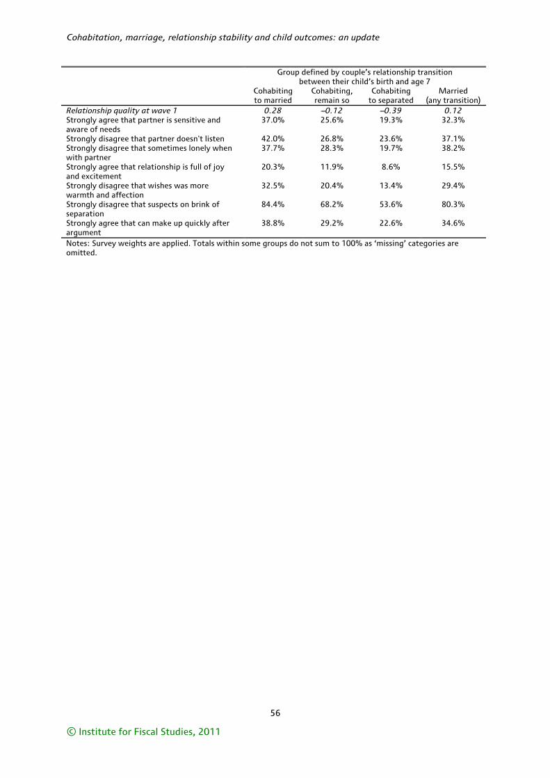
Cohabitation, marriage, relationship stability and child outcomes: an update
56
© Institute for Fiscal Studies, 2011
Group defined by couple’s relationship transition between their child’s birth and age 7
Cohabiting to married
Cohabiting, remain so
Cohabiting to separated
Married (any transition)
Relationship quality at wave 1 0.28 –0.12 –0.39 0.12 Strongly agree that partner is sensitive and aware of needs
37.0% 25.6% 19.3% 32.3%
Strongly disagree that partner doesn't listen 42.0% 26.8% 23.6% 37.1% Strongly disagree that sometimes lonely when with partner
37.7% 28.3% 19.7% 38.2%
Strongly agree that relationship is full of joy and excitement
20.3% 11.9% 8.6% 15.5%
Strongly disagree that wishes was more warmth and affection
32.5% 20.4% 13.4% 29.4%
Strongly disagree that suspects on brink of separation
84.4% 68.2% 53.6% 80.3%
Strongly agree that can make up quickly after argument
38.8% 29.2% 22.6% 34.6%
Notes: Survey weights are applied. Totals within some groups do not sum to 100% as ‘missing’ categories are omitted.
57
© Institute for Fiscal Studies, 2011
References
Acs, G. (2007), ‘Can we promote child well-being by promoting marriage?’, Journal of Marriage and Family, 69, 1326–44.
Acs, G., and S. Nelson (2002), ‘The kids are alright? Children’s well-being and the rise in cohabitation’, Urban Institute, Policy Brief / NSAF B-48.
Acs, G., and S. Nelson (2003), ‘Changes in family structure and child well-being: evidence from the 2002 National Survey of America’s Families’, Urban Institute, Research Report.
Acs, G., and S. Nelson (2004), ‘Should we get married in the morning? A profile of cohabiting couples with children’, Urban Institute, Assessing the New Federalism, Discussion Paper 04-01.
Andersson, G. (2002), ‘Children’s experience of family disruption and family formation: evidence from 16 FFS countries’, Demographic Research, 7, 343–64.
Artis, J. E. (2007), ‘Maternal cohabitation and child well-being among kindergarten children’, Journal of Marriage and the Family, 69, 222–36.
Benson, H. (2006), The Conflation of Marriage and Cohabitation in Government Statistics: A Denial of Difference Rendered Untenable by an Analysis of Outcomes, Bristol: Bristol Community Family Trust.
Benson, H. (2009), Married and Unmarried Family Breakdown: Key Statistics Explained, Bristol: Bristol Community Family Trust.
Björklund, A., D. Ginther and M. Sundström (2007), ‘Does marriage matter for children? Assessing the causal impact of legal marriage’, Institute for the Study of Labor (IZA), Discussion Paper 3189.
Brien, M. J., L. A. Lillard and S. Stern (2006), ‘Cohabitation, marriage, and divorce in a model of match quality’, International Economic Review, 47, 451–94.
Brown, S. L. (2004), ‘Family structure and child well-being: the significance of parental cohabitation’, Journal of Marriage and Family, 66, 351–67.
Bumpass, L., and H.-H. Lu (2000), ‘Trends in cohabitation and implications for children’s family contexts in the United States’, Population Studies, 54, 29–41.
Carneiro, P., C. Crawford and A. Goodman (2007), ‘The impact of early cognitive and non-cognitive skills on later outcomes’, Centre for the Economics of Education (CEE), Discussion Paper 92.
Conners, C. K. (1969), ‘A teacher rating scale for use in drug studies’, American Journal of Psychiatry, 126, 884–8.
Elliott, C. D., P. Smith and K. McCulloch (1996), British Ability Scales Second Edition (BAS II): Administration and Scoring Manual, London: NFER-Nelson.
Ermisch, J. (2005), ‘The puzzling rise of childbearing outside marriage’, in A. Heath, J. Ermisch and D. Gallie (eds), Understanding Social Change, Oxford: Oxford University Press.
Ermisch, J., and C. Pronzato (2008), ‘Intra-household allocation of resources: inferences from non-resident fathers’ child support payments’, Economic Journal, 118, 347–62.
Cohabitation, marriage, relationship stability and child outcomes: an update
58
© Institute for Fiscal Studies, 2011
Feinstein, L. (2000), ‘The relative economic importance of academic, psychological and behavioural attributes developed in childhood’, Centre for Economic Performance (CEP), Discussion Paper 443.
Fisher, H. (2010), ‘The health benefits of marriage: evidence using variation in marriage tax penalties’, work in progress (http://131.111.165.101/postgrad/hcf26/pubs/JobMarketPaperHayleyFisher.pdf).
Goodman, A., and E. Greaves (2010a), Cohabitation, Marriage and Child Outcomes, Commentary 114, London: Institute for Fiscal Studies (http://www.ifs.org.uk/publications/4823).
Goodman, A., and E. Greaves (2010b), ‘Cohabitation, marriage and relationship stability’, Institute for Fiscal Studies (IFS), Briefing Note 107 (http://www.ifs.org.uk/bns/bn107.pdf).
Graefe, D. R., and D. T. Lichter (1999), ‘Life course transitions of American children: parental cohabitation, marriage, and single motherhood’, Demography, 36, 205–17.
Heckman, J., J. Stixrud and S. Urzua (2006), ‘The effects of cognitive and noncognitive abilities on labour market outcomes and social behaviour’, Journal of Labor Economics, 24, 411–82.
Kiernan, K. (1999), ‘Childbearing outside marriage in Western Europe’, Population Trends, 98, 11–20.
Kiernan, K., and F. Mensah (2010), ‘Partnership trajectories, parent and child well-being’, in K. Hansen, H. Joshi and S. Dex (eds), Children of the 21st Century: The First Five Years, Bristol: Policy Press.
Manning, W. D. (2002), ‘The implications of cohabitation for children’s well-being’, in A. Booth and A. C. Crouter (eds), Just Living Together: Implications of Cohabitation for Children, Families, and Social Policy, Mahwah, NJ: Lawrence Erlbaum.
Manning, W. D., and S. Brown (2006), ‘Children’s economic well-being in married and cohabiting parent families’, Journal of Marriage and Family, 68, 345–62.
Manning, W. D., and K. A. Lamb (2003), ‘Adolescent well-being in cohabiting, married, and single-parent families’, Journal of Marriage and Family, 65, 876–93.
Manning, W. D., and D. T. Lichter (1996), ‘Parental cohabitation and children’s economic well-being’, Journal of Marriage and Family, 58, 998–1010.
Manning, W. D., P. J. Smock and D. Majumdar (2004), ‘The relative stability of cohabiting and marital unions for children’, Population Research and Policy Review, 23, 135–59.
McLanahan, S., and G. Sandefur (1994), Growing Up with a Single Parent: What Hurts, What Helps, Cambridge, MA: Harvard University Press.
Ribar, D. (2004), ‘What do social scientists know about the benefits of marriage? A review of quantitative methodologies’, Institute for the Study of Labor (IZA), Discussion Paper 998.
Smock, P. J., and S. Gupta (2002), ‘Cohabitation in contemporary North America’, in A. Booth and A. C. Crouter (eds), Just Living Together: Implications of Cohabitation for Children, Families, and Social Policy, Mahwah, NJ: Lawrence Erlbaum.