Coherence attribute at different spectral scales

Fangyu Li1 and Wenkai Lu2

Abstract

In general, we wish to interpret the most broadband data possible. However, broadband data do not alwaysprovide the best insight for seismic attribute analysis. Obviously, spectral bands contaminated by noise shouldbe eliminated. However, tuning gives rise to spectral bands with higher signal-to-noise ratios. To quantify geo-logic discontinuities in different scales, we combined spectral decomposition and coherence. Using spectraldecomposition, the spectral amplitudes corresponding to a given scale geologic discontinuity, as well as somesubtle features, which would otherwise be buried within the broadband seismic response, can be extracted. Weapplied this workflow to a 3D land data volume acquired over the Tarim Basin, Northwest China, where karstforms the principle reservoirs. We found that channels are better illuminated around 18 Hz, while subtle dis-continuities were better delineated around 25 Hz.

IntroductionStructural and stratigraphic discontinuities such as

channels, faults and fractures may provide lateral varia-tion in seismic expression. Seismic attributes suchas coherence delineate such lateral discontinuities, ac-celerate interpretation, and provide images of subtlefeatures that may otherwise have been overlooked.Al-Dossary and Marfurt (2006) use both long- andshort-wavelength curvature attributes from multispec-tral curvature estimation to enhance geologic featureshaving different scales. Sun et al. (2010) use discretefrequency coherence cubes in fracture detection andfind that high-frequency components can providegreater detail. Gao (2013) notices that more subtlestructural details in reservoirs are revealed using ahigher frequency wavelet as the spectral probe.

The seismic response of a given geologic feature isexpressed differently at different spectral bands. Often,a particular frequency component carries the informa-tion regarding structure and stratigraphy. Spectral de-composition methods map 1D signal into the 2D timeand frequency plane, generating amplitude and phasespectral components (Partyka et al., 1999; Castagnaet al., 2003). Extracting the spectral components at dif-ferent dominant frequencies may provide more preciseperspectives of given geologic structures. For example,the thickness of a channel and its spectral amplitude arestrongly correlated (Laughlin et al., 2002).

Time-frequency representation can be broadly di-vided into two classes: linear time-frequency and

bilinear (quadratic) time-frequency transforms. Chark-raborty and Okaya (1995) and Partyka et al. (1999) com-pute seismic spectral response using the short-timeFourier transform (STFT). Since then, other lineartime-frequency transforms, such as the continuouswavelet transform (Sinha et al., 2005) and the Stransform (Matos et al., 2005) as well as bilineartime-frequency transforms, such as the smoothedpseudo-Wigner-Ville distribution (Li and Zheng, 2008)have been introduced to improve the temporal dataanalysis and frequency resolution. Fourier transformrepresentation of the convolution between the signaland the time-frequency atom is equivalent to a suiteof narrow band-pass filters, resulting in a suite of com-plex spectra (Qian, 2002). In contrast, bilinear trans-forms based on quadratic energy do not generatephase information. Spectral magnitude of the jointtime-frequency spectrum is routinely used in reservoircharacterization (Liu and Marfurt, 2007), hydrocarbondetection (Castagna et al., 2003; Lu and Li, 2013), andmeasuring tuning and attenuation effects (Partyka et al.,1999). However, to delineate lateral stratigraphic dis-continuities (Matos et al., 2011), we need the spectralphase component of the joint time-frequency distribu-tion. Fahmy et al. (2005) apply a band-pass filter usingthe most significant frequency bandwidth of seismicdata for reservoir illumination. Hardage (2009) demon-strates that frequency-constrained seismic data can pro-vide improved images of geologic systems.

1Formerly Tsinghua University, Department of Automation, Beijing, China; presently The University of Oklahoma, ConocoPhillips School ofGeology and Geophysics, Norman, Oklahoma, USA. E-mail: fangyu.li@ou.edu.

2Tsinghua University, State Key Laboratory of Intelligent Technology and Systems, Tsinghua National Laboratory for Information Science andTechnology, Department of Automation, Beijing, China. E-mail: lwkmf@mail.tsinghua.edu.cn.

Manuscript received by the Editor 18 June 2013; revised manuscript received 19 October 2013. This paper appears in Interpretation, Vol. 2, No. 1(February 2014); p. 1–8, 10 FIGS.

http://dx.doi.org/10.1190/INT-2013-0089.1. © 2013 Society of Exploration Geophysicists and American Association of Petroleum Geologists. All rights reserved.

t

Special section: Seismic attributes

11

Estimates of seismic coherence (Bahorich andFarmer, 1995; Marfurt et al., 1998; Gerstzenkorn andMarfurt, 1999; Lu et al., 2005) measure changes in wave-form and provide a quantitative measure of geologicdiscontinuities. In general, most interpreters applycoherence to the final processed, broadbanded data

(Chopra and Marfurt, 2007). Coherence can be com-puted from the real seismic or from the analytic seismicdata (Taner et al., 1979). Using the analytic trace cansharpen discontinuities (Guo et al., 2009). For thisreason, we adopt linear rather than quadratic time-frequency analysis methods to generate complex spec-tra in our work.

In this paper, we combine spectral decomposition,which extracts complex spectral amplitudes from thefrequency bands of interest, and complex coherencecomputation to map discontinuities at different vertical

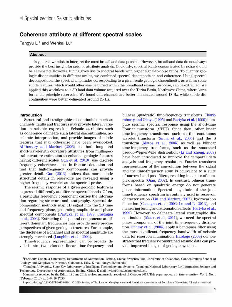
Figure 1. A seismic trace and its derived attributes: (a) themeasured seismic trace (solid line) and the instantaneousenvelope (dotted line), (b) instantaneous phase, and (c) ascaled version of the measured seismic trace (light line)and the cosine of the instantaneous phase (heavy line).

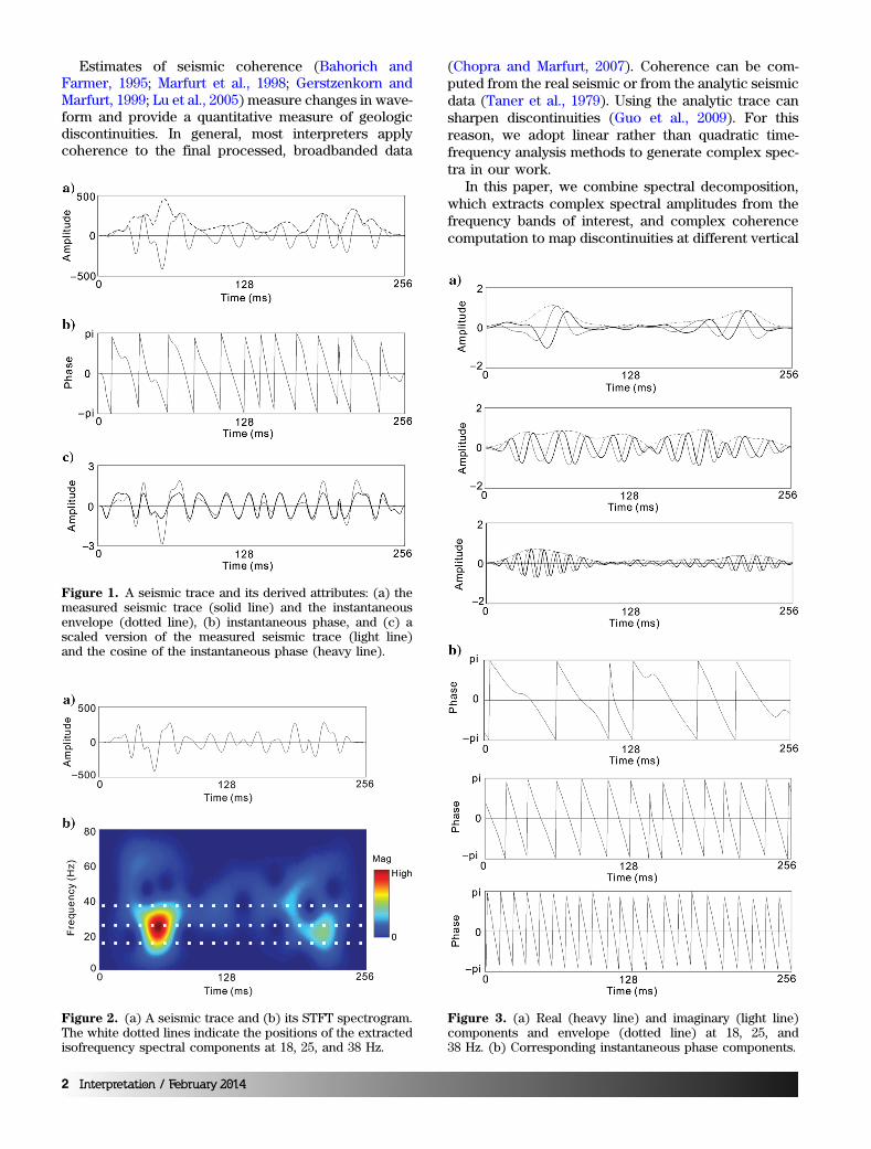
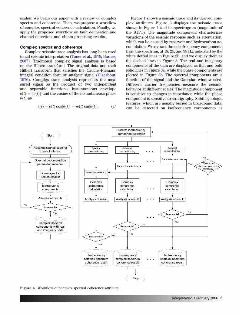
Figure 2. (a) A seismic trace and (b) its STFT spectrogram.The white dotted lines indicate the positions of the extractedisofrequency spectral components at 18, 25, and 38 Hz.

Figure 3. (a) Real (heavy line) and imaginary (light line)components and envelope (dotted line) at 18, 25, and38 Hz. (b) Corresponding instantaneous phase components.

2 Interpretation / February 2014

scales. We begin our paper with a review of complexspectra and coherence. Then, we propose a workflowof complex spectral coherence calculation. Finally, weapply the proposed workflow on fault delineation andchannel detection, and obtain promising results.

Complex spectra and coherenceComplex seismic trace analysis has long been used

to aid seismic interpretation (Taner et al., 1979; Barnes,2007). Traditional complex signal analysis is basedon the Hilbert transform. The original data and theirHilbert transform that satisfies the Cauchy-Riemannintegral condition form an analytic signal (Claerbout,1976). Complex trace analysis represents the mea-sured signal as the product of two independentand separable functions: instantaneous envelopeeðtÞ ¼ kcðtÞk and the cosine of the instantaneous phaseθðtÞ as

cðtÞ ¼ eðtÞ cos½θðtÞ� þ ieðtÞ sin½θðtÞ�: (1)

Figure 1 shows a seismic trace and its derived com-plex attributes. Figure 2 displays the seismic traceshown in Figure 1 and its spectrogram (magnitude ofthe STFT). The magnitude component characterizesvariations of the seismic response such as attenuation,which can be caused by reservoir and hydrocarbon ac-cumulation. We extract three isofrequency componentsfrom the spectrum, at 18, 25, and 38 Hz, indicated by thewhite dotted lines in Figure 2b, and we display them asthe dashed lines in Figure 3. The real and imaginarycomponents of the data are displayed as thin and boldsolid lines in Figure 3a, while the phase components areplotted in Figure 3b. The spectral components are afunction of the signal and the Gaussian window used.Different carrier frequencies measure the seismicbehavior at different scales. The magnitude componentis sensitive to changes in impedance while the phasecomponent is sensitive to stratigraphy. Subtle geologicfeatures, which are usually buried in broadband data,can be detected on isofrequency components as

Figure 4. Workflow of complex spectral coherence attribute.

Interpretation / February 2014 3

the disturbance when other frequencies have beensuppressed.

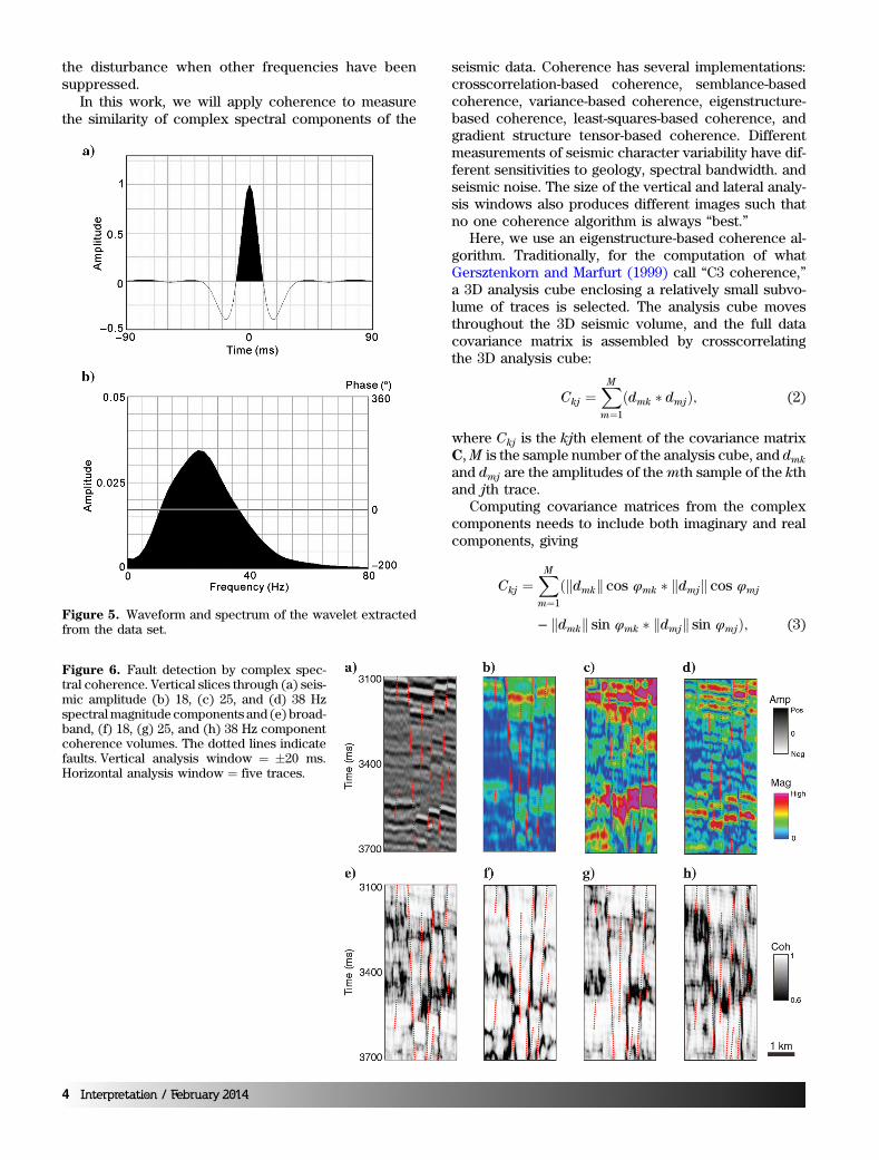
In this work, we will apply coherence to measurethe similarity of complex spectral components of the

seismic data. Coherence has several implementations:crosscorrelation-based coherence, semblance-basedcoherence, variance-based coherence, eigenstructure-based coherence, least-squares-based coherence, andgradient structure tensor-based coherence. Differentmeasurements of seismic character variability have dif-ferent sensitivities to geology, spectral bandwidth. andseismic noise. The size of the vertical and lateral analy-sis windows also produces different images such thatno one coherence algorithm is always “best.”

Here, we use an eigenstructure-based coherence al-gorithm. Traditionally, for the computation of whatGersztenkorn and Marfurt (1999) call “C3 coherence,”a 3D analysis cube enclosing a relatively small subvo-lume of traces is selected. The analysis cube movesthroughout the 3D seismic volume, and the full datacovariance matrix is assembled by crosscorrelatingthe 3D analysis cube:

Ckj ¼XM

m¼1

ðdmk � dmjÞ; (2)

where Ckj is the kjth element of the covariance matrixC,M is the sample number of the analysis cube, and dmkand dmj are the amplitudes of themth sample of the kthand jth trace.

Computing covariance matrices from the complexcomponents needs to include both imaginary and realcomponents, giving

Ckj ¼XM

m¼1

ðkdmkk cos φmk � kdmjk cos φmj

− kdmkk sin φmk � kdmjk sin φmjÞ; (3)Figure 5. Waveform and spectrum of the wavelet extractedfrom the data set.

Figure 6. Fault detection by complex spec-tral coherence. Vertical slices through (a) seis-mic amplitude (b) 18, (c) 25, and (d) 38 Hzspectralmagnitude components and (e) broad-band, (f) 18, (g) 25, and (h) 38 Hz componentcoherence volumes. The dotted lines indicatefaults. Vertical analysis window ¼ �20 ms.Horizontal analysis window ¼ five traces.

4 Interpretation / February 2014

where kdmnk is the magnitude, φmn is the phase of thecomplex spectral components, and kdmnk sinφmn andkdmnk cosφmn are the imaginary and real components,respectively. During 3D attribute computation, Gersz-tenkorn (2012) uses a similar way to facilitate the rep-resentation for matrix entries.

ApplicationThe entire workflow of complex spectral coherence

calculation is displayed in Figure 4. To obtain isofre-quency components at different frequencies, thesespectral components should be checked for both reso-lution and artifact suppression. Large windows may bemore “stable,” but they may mix stratigraphy. Smallwindows may be too small to contain a period of inter-est. After obtaining complex spectral components withboth real and imaginary parts, the selected discrete iso-frequency components are used as input to coherence.Because of thin bed tuning, some spectral componentswill illuminate geology better than others, as Fahmyet al. (2005) find with AVO analysis. Other componentsmay be dominated by noise and should be rejected, asHardage (2009) shows.

Figure 5 shows the waveform and the spectrum ofthe wavelet extracted from our well tie. This waveletis zero phase, centered at about 25 Hz, so we will illus-trate our analysis with 10, 25, and 40 Hz frequencies. In

this application, we used STFT as the linear transformand the eigenstucture-based algorithm as the coherenceattribute.

Fault DelineationFigure 6 displays a fault detection example. Figure 6a

shows seismic amplitude, Figure 6b–6d shows the cor-responding vertical slices through 10, 25, and 40 Hzspectral magnitude components, while vertical slicesthrough the coherence volumes from the original(“broadband”) shown in Figure 6e and Figure 6f–6hare the 10, 25, and 40 Hz spectral component coherenceprofiles, respectively. Red dotted lines indicate normalfaults. But, the broadband coherence result delineatesthe main fault on the right but not the one on the left. Incontrast, the low-frequency spectral coherence delin-eates both main faults most clearly, while the middle-and high-frequency spectral coherence highlightssmaller discontinuities near the faults that we interpretto be conjugate faults. The 10 Hz component of thecoherence attribute shows more continuous imagesof large scale features.

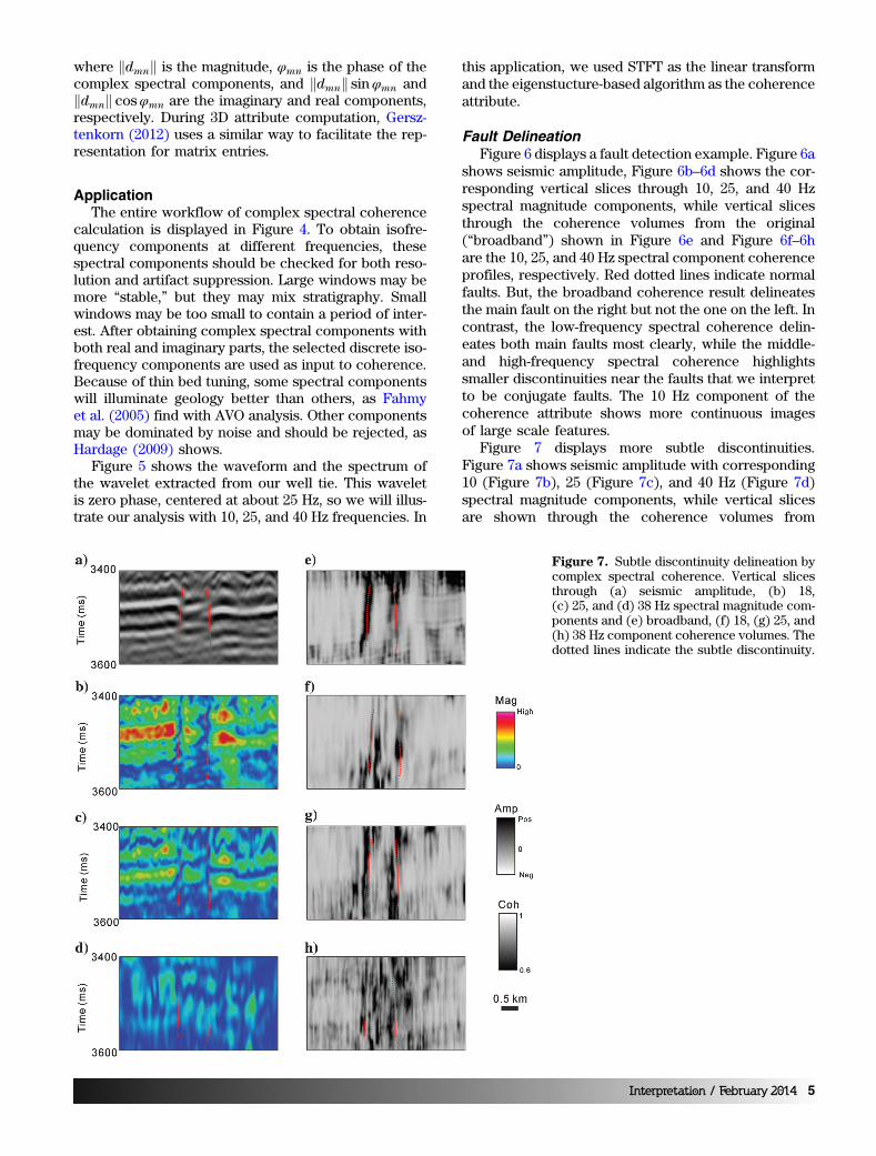
Figure 7 displays more subtle discontinuities.Figure 7a shows seismic amplitude with corresponding10 (Figure 7b), 25 (Figure 7c), and 40 Hz (Figure 7d)spectral magnitude components, while vertical slicesare shown through the coherence volumes from

Figure 7. Subtle discontinuity delineation bycomplex spectral coherence. Vertical slicesthrough (a) seismic amplitude, (b) 18,(c) 25, and (d) 38 Hz spectral magnitude com-ponents and (e) broadband, (f) 18, (g) 25, and(h) 38 Hz component coherence volumes. Thedotted lines indicate the subtle discontinuity.

Interpretation / February 2014 5

broadband (Figure 7e), 10 (Figure 7f), 25 (Figure 7g),and 40 Hz (Figure 7h) spectral components, respec-tively. The fracture lineaments in Figure 7g correlatewith textures with faulting we expect to occur withcompression.

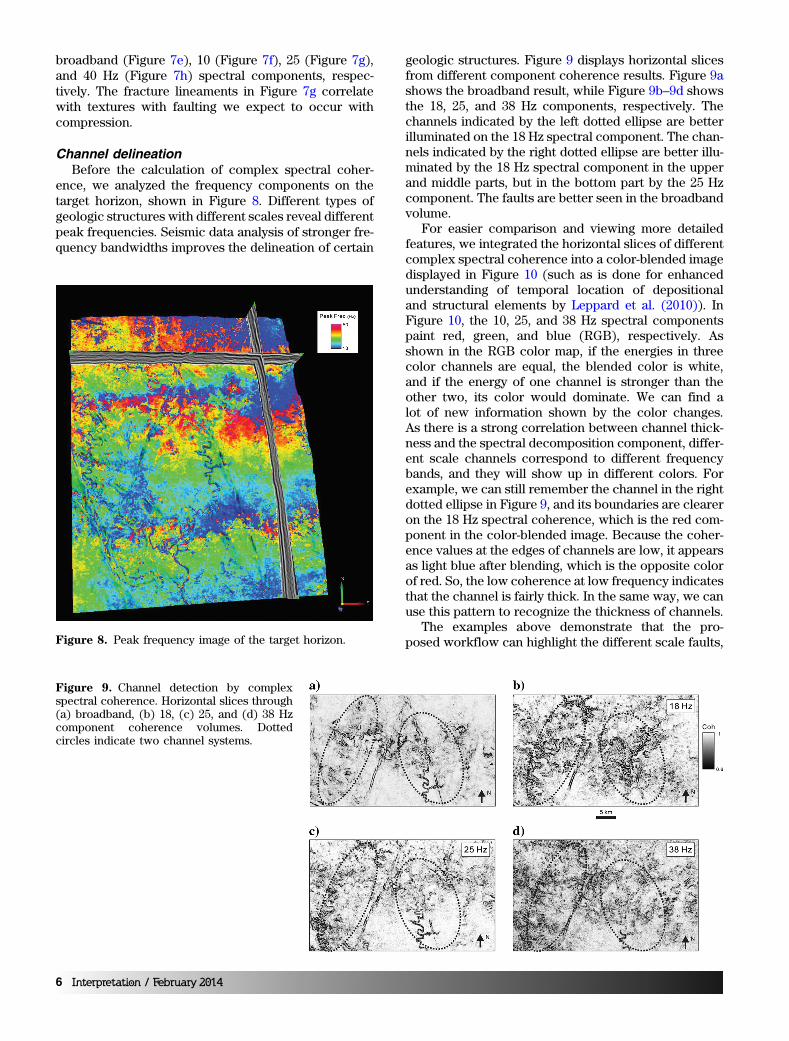
Channel delineationBefore the calculation of complex spectral coher-

ence, we analyzed the frequency components on thetarget horizon, shown in Figure 8. Different types ofgeologic structures with different scales reveal differentpeak frequencies. Seismic data analysis of stronger fre-quency bandwidths improves the delineation of certain

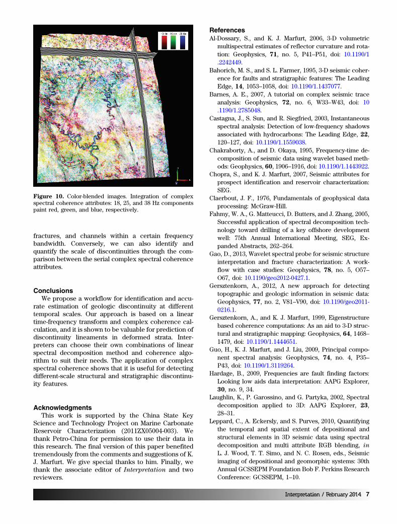
geologic structures. Figure 9 displays horizontal slicesfrom different component coherence results. Figure 9ashows the broadband result, while Figure 9b–9d showsthe 18, 25, and 38 Hz components, respectively. Thechannels indicated by the left dotted ellipse are betterilluminated on the 18 Hz spectral component. The chan-nels indicated by the right dotted ellipse are better illu-minated by the 18 Hz spectral component in the upperand middle parts, but in the bottom part by the 25 Hzcomponent. The faults are better seen in the broadbandvolume.

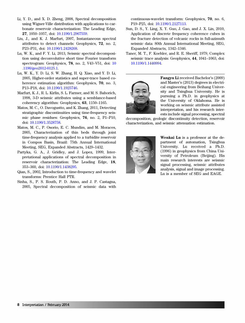
For easier comparison and viewing more detailedfeatures, we integrated the horizontal slices of differentcomplex spectral coherence into a color-blended imagedisplayed in Figure 10 (such as is done for enhancedunderstanding of temporal location of depositionaland structural elements by Leppard et al. (2010)). InFigure 10, the 10, 25, and 38 Hz spectral componentspaint red, green, and blue (RGB), respectively. Asshown in the RGB color map, if the energies in threecolor channels are equal, the blended color is white,and if the energy of one channel is stronger than theother two, its color would dominate. We can find alot of new information shown by the color changes.As there is a strong correlation between channel thick-ness and the spectral decomposition component, differ-ent scale channels correspond to different frequencybands, and they will show up in different colors. Forexample, we can still remember the channel in the rightdotted ellipse in Figure 9, and its boundaries are cleareron the 18 Hz spectral coherence, which is the red com-ponent in the color-blended image. Because the coher-ence values at the edges of channels are low, it appearsas light blue after blending, which is the opposite colorof red. So, the low coherence at low frequency indicatesthat the channel is fairly thick. In the same way, we canuse this pattern to recognize the thickness of channels.

The examples above demonstrate that the pro-posed workflow can highlight the different scale faults,Figure 8. Peak frequency image of the target horizon.

Figure 9. Channel detection by complexspectral coherence. Horizontal slices through(a) broadband, (b) 18, (c) 25, and (d) 38 Hzcomponent coherence volumes. Dottedcircles indicate two channel systems.

6 Interpretation / February 2014

fractures, and channels within a certain frequencybandwidth. Conversely, we can also identify andquantify the scale of discontinuities through the com-parison between the serial complex spectral coherenceattributes.

ConclusionsWe propose a workflow for identification and accu-

rate estimation of geologic discontinuity at differenttemporal scales. Our approach is based on a lineartime-frequency transform and complex coherence cal-culation, and it is shown to be valuable for prediction ofdiscontinuity lineaments in deformed strata. Inter-preters can choose their own combinations of linearspectral decomposition method and coherence algo-rithm to suit their needs. The application of complexspectral coherence shows that it is useful for detectingdifferent-scale structural and stratigraphic discontinu-ity features.

AcknowledgmentsThis work is supported by the China State Key

Science and Technology Project on Marine CarbonateReservoir Characterization (2011ZX05004-003). Wethank Petro-China for permission to use their data inthis research. The final version of this paper benefitedtremendously from the comments and suggestions of K.J. Marfurt. We give special thanks to him. Finally, wethank the associate editor of Interpretation and tworeviewers.

ReferencesAl-Dossary, S., and K. J. Marfurt, 2006, 3-D volumetric

multispectral estimates of reflector curvature and rota-tion: Geophysics, 71, no. 5, P41–P51, doi: 10.1190/1.2242449.

Bahorich, M. S., and S. L. Farmer, 1995, 3-D seismic coher-ence for faults and stratigraphic features: The LeadingEdge, 14, 1053–1058, doi: 10.1190/1.1437077.

Barnes, A. E., 2007, A tutorial on complex seismic traceanalysis: Geophysics, 72, no. 6, W33–W43, doi: 10.1190/1.2785048.

Castagna, J., S. Sun, and R. Siegfried, 2003, Instantaneousspectral analysis: Detection of low-frequency shadowsassociated with hydrocarbons: The Leading Edge, 22,120–127, doi: 10.1190/1.1559038.

Chakraborty, A., and D. Okaya, 1995, Frequency-time de-composition of seismic data using wavelet based meth-ods: Geophysics, 60, 1906–1916, doi: 10.1190/1.1443922.

Chopra, S., and K. J. Marfurt, 2007, Seismic attributes forprospect identification and reservoir characterization:SEG.

Claerbout, J. F., 1976, Fundamentals of geophysical dataprocessing: McGraw-Hill.

Fahmy, W. A., G. Matteucci, D. Butters, and J. Zhang, 2005,Successful application of spectral decomposition tech-nology toward drilling of a key offshore developmentwell: 75th Annual International Meeting, SEG, Ex-panded Abstracts, 262–264.

Gao, D., 2013, Wavelet spectral probe for seismic structureinterpretation and fracture characterization: A work-flow with case studies: Geophysics, 78, no. 5, O57–O67, doi: 10.1190/geo2012-0427.1.

Gersztenkorn, A., 2012, A new approach for detectingtopographic and geologic information in seismic data:Geophysics, 77, no. 2, V81–V90, doi: 10.1190/geo2011-0216.1.

Gersztenkorn, A., and K. J. Marfurt, 1999, Eigenstructurebased coherence computations: As an aid to 3-D struc-tural and stratigraphic mapping: Geophysics, 64, 1468–1479, doi: 10.1190/1.1444651.

Guo, H., K. J. Marfurt, and J. Liu, 2009, Principal compo-nent spectral analysis: Geophysics, 74, no. 4, P35–P43, doi: 10.1190/1.3119264.

Hardage, B., 2009, Frequencies are fault finding factors:Looking low aids data interpretation: AAPG Explorer,30, no. 9, 34.

Laughlin, K., P. Garossino, and G. Partyka, 2002, Spectraldecomposition applied to 3D: AAPG Explorer, 23,28–31.

Leppard, C., A. Eckersly, and S. Purves, 2010, Quantifyingthe temporal and spatial extent of depositional andstructural elements in 3D seismic data using spectraldecomposition and multi attribute RGB blending, inL. J. Wood, T. T. Simo, and N. C. Rosen, eds., Seismicimaging of depositional and geomorphic systems: 30thAnnual GCSSEPM Foundation Bob F. Perkins ResearchConference: GCSSEPM, 1–10.

Figure 10. Color-blended images. Integration of complexspectral coherence attributes: 18, 25, and 38 Hz componentspaint red, green, and blue, respectively.

Interpretation / February 2014 7

Li, Y. D., and X. D. Zheng, 2008, Spectral decompositionusing Wigner-Ville distribution with applications to car-bonate reservoir characterization: The Leading Edge,27, 1050–1057, doi: 10.1190/1.2967559.

Liu, J., and K. J. Marfurt, 2007, Instantaneous spectralattributes to detect channels: Geophysics, 72, no. 2,P23–P31, doi: 10.1190/1.2428268.

Lu, W. K., and F. Y. Li, 2013, Seismic spectral decomposi-tion using deconvolutive short time Fourier transformspectrogram: Geophysics, 78, no. 2, V43–V51, doi: 10.1190/geo2012-0125.1.

Lu, W. K., Y. D. Li, S. W. Zhang, H. Q. Xiao, and Y. D. Li,2005, Higher-order statistics and super-trace based co-herence estimation algorithm: Geophysics, 70, no. 3,P13–P18, doi: 10.1190/1.1925746.

Marfurt, K. J., R. L. Kirlin, S. L. Farmer, and M. S. Bahorich,1998, 3-D seismic attributes using a semblance-basedcoherency algorithm: Geophysics, 63, 1150–1165.

Matos, M. C., O. Davogustto, and K. Zhang, 2011, Detectingstratigraphic discontinuities using time-frequency seis-mic phase residues: Geophysics, 76, no. 2, P1–P10,doi: 10.1190/1.3528758.

Matos, M. C., P. Osorio, E. C. Mundim, and M. Moraces,2005, Characterization of thin beds through jointtime-frequency analysis applied to a turbidite reservoirin Compos Basin, Brazil: 75th Annual InternationalMeeting, SEG, Expanded Abstracts, 1429–1432.

Partyka, G. A., J. Gridley, and J. Lopez, 1999, Inter-pretational applications of spectral decomposition inreservoir characterization: The Leading Edge, 18,353–360, doi: 10.1190/1.1438295.

Qian, S., 2002, Introduction to time-frequency and wavelettransforms: Prentice Hall PTR.

Sinha, S., P. S. Routh, P. D. Anno, and J. P. Castagna,2005, Spectral decomposition of seismic data with

continuous-wavelet transform: Geophysics, 70, no. 6,P19–P25, doi: 10.1190/1.2127113.

Sun, D. S., Y. Ling, X. Y. Guo, J. Gao, and J. X. Lin, 2010,Application of discrete frequency coherence cubes inthe fracture detection of volcanic rocks in full-azimuthseismic data: 80th Annual International Meeting, SEG,Expanded Abstracts, 1342–1346.

Taner, M. T., F. Koehler, and R. E. Sheriff, 1979, Complexseismic trace analysis: Geophysics, 44, 1041–1063, doi:10.1190/1.1440994.

Fangyu Li received Bachelor’s (2009)and Master’s (2013) degrees in electri-cal engineering from Beihang Univer-sity and Tsinghua University. He ispursuing a Ph.D. in geophysics atthe University of Oklahoma. He isworking on seismic attribute assistedinterpretation, and his research inter-ests include signal processing, spectral

decomposition, geologic discontinuity detection, reservoircharacterization, and seismic attenuation estimation.

Wenkai Lu is a professor at the de-partment of automation, TsinghuaUniversity. Lu received a Ph.D.(1996) in geophysics from China Uni-versity of Petroleum (Beijing). Hismain research interests are seismicsignal processing, seismic attributesanalysis, signal and image processing.Lu is a member of SEG and EAGE.

8 Interpretation / February 2014