coherent and non-coherent ultra-wideband...
TRANSCRIPT
Ph.D. Dissertation
Coherent and Non-Coherent
Ultra-Wideband Communications
Author: Jose A. Lopez-Salcedo
Advisor: Prof. Gregori Vazquez Grau
Department of Signal Theory and CommunicationsUniversitat Politecnica de Catalunya
Barcelona, March 28th, 2007

Abstract
Short-range wireless communication has become an essential part of everyday life thanks to the
enormous growth in the deployment of wireless local and personal area networks. However,
traditional wireless technology cannot meet the requirements of upcoming wireless services that
demand high-data rates to operate. This issue has motivated an unprecedented resurgence of
ultra-wideband (UWB) technology, a transmission technique that is based on the emission of sub-
nanosecond pulses with a very low transmitted power. Because of the particular characteristics
of UWB signals, very high data rates can be provided with multipath immunity and high
penetration capabilities.
Nevertheless, formidable challenges must be faced in order to fulfill the expectations of UWB
technology. One of the most important challenges is to cope with the overwhelming distortion
introduced by the intricate propagation physics of UWB signals. In addition to this, UWB
antennas behave like direction-sensitive filters such that the signal driving the transmit antenna,
the electric far field, and the signal across the receiver load, they all may differ considerably in
wave shape. As a result, the well-known and popular concept of matched filter correlation
cannot be implemented unless high computational complexity is available for perfect waveform
estimation.
The lack of knowledge about the received waveform leads UWB receivers to be implemented
under a coherent or non-coherent approach depending on a tradeoff between waveform estimation
complexity and system performance. On the one hand, coherent receivers provide the reference
benchmark in the sense that they have ideally perfect knowledge of the end-to-end channel
response and thus, optimal performance is achieved. On the other hand, non-coherent receivers
appear as a low-cost and low-power consumption alternative since channel estimation is not
considered and thus, suboptimal performance is expected.
In the present dissertation, both coherent and non-coherent receivers for UWB communi-
cations are analyzed from a twofold perspective. In the first part of the thesis, an information
theoretic approach is adopted to understand the implications of coherent and non-coherent re-
ception. This is done by analyzing the achievable data rates for which reliable communication is
possible in the presence and in the absence of channel state information. The simulation results
i

ii Abstract
show a different behavior when evaluating spectral efficiency of coherent and non-coherent re-
ceivers under the wideband regime. For this reason, and in order to shed some light on this issue,
closed-form expressions are derived to allow an analytical study of the asymptotic behavior of
constellation-constrained capacity.
In the second part of the thesis, the emphasis is placed on the design of signal processing tech-
niques for carrying out the basic tasks of an UWB receiver. For the case of coherent receivers,
a maximum likelihood waveform estimation technique is proposed based on the exploitation of
second-order statistics. One of the key features of the proposed technique is that it establishes
a clear link between maximum likelihood waveform estimation and correlation matching tech-
niques. Moreover, the proposed method can be understood as a principal component analysis
that compresses the likelihood function with information regarding the signal subspace of the re-
ceived signal. As a result, significant reduction in the computational burden is obtained through
a tradeoff between bias and variance.
For the case of non-coherent receivers, the problems of symbol detection and signal synchro-
nization are addressed from a waveform-independent perspective. The framework of waveform-
independent symbol detection is derived for the case of correlated and uncorrelated scenar-
ios, and low-complexity implementations are proposed based on the maximization of the Jef-
freys divergence measure. As for the synchronization problem, a nondata-aided and waveform-
independent technique is proposed for the frame-timing acquisition of the received signal. Next,
a low-complexity implementation is proposed based on the multifamily likelihood ratio testing
by understanding the frame-timing acquisition of UWB signals as a problem of model order
detection.

Resumen
Las comunicaciones inalambricas de corto alcance se han convertido en una parte imprescindible
de la vida diaria gracias a la extraordinaria expansion de las redes inalambricas de area local
y personal. Sin embargo, la tecnologıa inalambrica actual no es capaz de satisfacer los req-
uisitos de alta velocidad que demandan los servicios de nueva generacion. Este problema ha
motivado la reaparicion de la tecnologıa de banda ultra-ancha o ultra-wideband (UWB), una
tecnologıa basada en la emision de pulsos de baja potencia cuya duracion temporal es infe-
rior al nanosegundo. Debido a las particulares caracterısticas de las senales UWB, es posible
conseguir velocidades de transmision muy elevadas con inmunidad al efecto multicamino y alta
penetrabilidad en materiales.
A pesar de ello, existen formidables desafıos que han de afrontarse si se pretende cumplir
con las expectativas que la tecnologıa UWB ha generado. En concreto, uno de los desafıos mas
importantes es el relacionado con la severa distorsion que introduce la propagacion de senales
de banda ultra-ancha. En este sentido, se ha comprobado que la senal que alimenta la antena de
UWB, la senal del campo electrico lejano y la senal recibida en la carga de la antena receptora,
todas ellas suelen diferir de manera considerable en su forma de onda. Como consecuencia, el
tradicional concepto de filtrado adaptado se hace inviable a no ser que se disponga de una gran
capacidad de calculo y complejidad hardware para llevar a cabo una estimacion precisa de la
forma de onda recibida.
El desconocimiento de la forma de onda recibida conduce a la implementacion de receptores
de UWB bajo una perspectiva coherente o no-coherente, dependiendo de un compromiso entre
complejidad hardware y prestaciones del sistema. Por un lado, los receptores coherentes imple-
mentan estimacion de forma de onda y por lo tanto proporcionan las mejores prestaciones al
asumir un conocimiento preciso de las condiciones de propagacion. Por otro lado, los receptores
no-coherentes aparecen como una alternativa sub-optima de bajo coste y bajo consumo al no
implementar estimacion de canal.
En la presente tesis, los receptores coherentes y no-coherentes para senales de UWB son anal-
izados desde una doble perspectiva. En la primera parte de la tesis se adopta un planteamiento
de teorıa de la informacion con el objetivo de comprender las implicaciones de la deteccion coher-
iii
iv Resumen
ente y no-coherente. Ello se consigue mediante el analisis de los lımites teoricos para los cuales es
posible una comunicacion fiable sin errores en presencia y en ausencia de informacion acerca del
estado del canal. Los resultados de simulacion muestran un comportamiento diferente entre los
receptores coherentes y no-coherentes cuando ambos son evaluados en terminos de su eficiencia
espectral bajo el regimen de banda ancha. Por esta razon, y con el objetivo con profundizar
en este problema, se proponen expresiones cerradas para el analisis teorico del comportamiento
asintotico de la capacidad de canal sujeta a una constelacion discreta de entrada.
En la segunda parte de la tesis, el enfasis se centra en el diseno de tecnicas de procesado de
senal para llevar a cabo las tareas basicas de un receptor de UWB. Para el caso de receptores
coherentes, se propone una tecnica de estimacion de forma de onda basada en estadısticos de
segundo orden. Una de las caracterısticas principales de la tecnica propuesta es que establece
una relacion clara entre el criterio de maxima verosimilitud y las tecnicas de correlation match-
ing. Ademas de ello, el metodo propuesto puede ser entendido como una tecnica de analisis de
componentes principales (PCA) que comprime la funcion de maxima verosimilitud con la infor-
macion disponible acerca del subespacio de senal. Como resultado, se obtiene una significativa
reduccion de complejidad mediante un compromiso entre sesgo y varianza.
Para el caso de receptores no-coherentes, se plantean los problemas de deteccion no-coherente
y sincronizacion no asistida. Por lo que respecta al problema de deteccion, se ha desarrollado
un marco teorico para implementar de manera optima la decision de sımbolo en escenarios
con scattering correlado o incorrelado. Se propone una implementacion de baja complejidad
basada en la maximizacion de la divergencia de Jeffreys. Por lo que respecta al problema
de sincronizacion, se propone una tecnica de adquisicion de timing de trama no asistida por
datos e independiente de la forma de onda recibida. En este caso se propone tambien una
implementacion de baja complejidad basada en el criterio de multifamily likelihood ratio testing
mediante la interpretacion de la adquisicion de timing como un problema de deteccion de orden
del modelo.

Agradecimientos
Estas primeras lıneas ponen punto y final a mis anos de doctorado, un antes y un despues en
una de las etapas de mi vida que sin duda recordare con mas carino. Una vez llegados al final,
es de justicia volver la vista atras para mostrar mi mas sincero agradecimiento y admiracion a
todos aquellos que han hecho posible que recorriera este largo pero apasionante camino.
Mi primer agradecimiento no puede ser para otra persona mas que para Gregori, copartıcipe
de esta tesis y persona excepcional alla donde las haya. Una persona de la que sigo aprendiendo
cada dıa y de la que agradezco el apoyo y confianza que ha tenido en mı tanto a nivel personal
como a nivel profesional. Mi agradecimiento tambien para Jaume por su inestimable ayuda y su
particular sentido de la intuicion. Una gran persona en el sentido mas literal de la palabra. De
manera similar, no puedo olvidar tampoco el tiempo que estuve trabajando con Xell al comienzo
de mi etapa de doctorado. De ella guardo un recuerdo muy especial y a ella le debo todo lo
que aprendı sobre codificacion. Francesc Rey y Xavi Villares tambien merecen una mencion
especial. Ellos han sido de alguna manera mis hermanos mayores durante todo este tiempo y
en ellos siempre he encontrado consejos y animos en los momentos difıciles.
Como no, quisiera tambien mostrar mi agradecimiento a los becarios de doctorado con los
que he tenido el placer de compartir esta experiencia. A los que todavıa estan ahı y a los
que ya se han ido. A todos ellos mi agradecimiento por todo lo que hemos compartido juntos.
Nombrarlos a todos serıa excesivo, pero ellos saben quienes son y por que los admiro.
Finalmente, agradecer tambien el apoyo que me han brindado siempre mi familia y Ester.
Despues de mi dedicacion a la carrera, quiero expresar mi gratitud por su compresion y paciencia
a lo largo de este nuevo ciclo de otros cinco anos de doctorado que ahora termina. Espero poderles
devolver pronto el tiempo que no les he podido dedicar durante estos casi diez anos de estudios.
Jose A. Lopez-Salcedo
7 de febrero de 2007
Este trabajo ha sido parcialmente financiado por el Ministerio de Educacion y Ciencia a traves del programa
de Formacion de Personal Investigador (F.P.I.) mediante la beca FP-2001-2639.
vii


Contents
Abstract i
Resumen iii
List of Figures xviii
List of Tables xix
Notation xxi
Acronyms xxv
1 Introduction 1
1.1 Motivation and Objectives . . . . . . . . . . . . . . . . . . . . . . . . . . . . . . 2
1.2 Thesis Outline . . . . . . . . . . . . . . . . . . . . . . . . . . . . . . . . . . . . . 2
1.3 Research Contributions . . . . . . . . . . . . . . . . . . . . . . . . . . . . . . . . 5
2 Overview of UWB Technology 9
2.1 Introduction . . . . . . . . . . . . . . . . . . . . . . . . . . . . . . . . . . . . . . . 9
2.2 A Brief Historical Review . . . . . . . . . . . . . . . . . . . . . . . . . . . . . . . 9
2.3 Regulation and Standardization of UWB Technology . . . . . . . . . . . . . . . . 11
2.3.1 Regulations on the emission limits of UWB signals . . . . . . . . . . . . . 12
2.3.2 Standardization within the IEEE . . . . . . . . . . . . . . . . . . . . . . . 14
2.3.3 Standardization controversy within industry . . . . . . . . . . . . . . . . . 15
ix

x Contents
2.4 Fundamentals of UWB Technology . . . . . . . . . . . . . . . . . . . . . . . . . . 16
2.4.1 Key features of UWB technology . . . . . . . . . . . . . . . . . . . . . . . 16
2.4.2 Signaling formats . . . . . . . . . . . . . . . . . . . . . . . . . . . . . . . . 18
2.4.3 Standardized channel modeling . . . . . . . . . . . . . . . . . . . . . . . . 19
2.4.4 Pulse distortion . . . . . . . . . . . . . . . . . . . . . . . . . . . . . . . . . 21
2.5 Applications of UWB Technology . . . . . . . . . . . . . . . . . . . . . . . . . . . 23
2.6 Challenges in UWB Technology . . . . . . . . . . . . . . . . . . . . . . . . . . . . 24
2.6.1 Hardware implementation challenges . . . . . . . . . . . . . . . . . . . . . 24
2.6.2 Signal processing challenges . . . . . . . . . . . . . . . . . . . . . . . . . . 26
3 Performance Limits of Coherent and Non-coherent Ultra-Wideband Commu-
nications 29
3.1 Introduction . . . . . . . . . . . . . . . . . . . . . . . . . . . . . . . . . . . . . . . 29
3.2 Modulation Formats for UWB Communication Systems . . . . . . . . . . . . . . 30
3.2.1 PAM or PPM modulation? . . . . . . . . . . . . . . . . . . . . . . . . . . 30
3.2.2 Signal model for PPM modulation . . . . . . . . . . . . . . . . . . . . . . 31
3.3 Review of Information Theoretic Results for Wideband Communications . . . . . 33
3.3.1 Power efficiency in the wideband regime . . . . . . . . . . . . . . . . . . . 33
3.3.2 Asymptotic performance over fading channels . . . . . . . . . . . . . . . . 34
3.3.3 Wideband optimality and minimum Eb/N0 . . . . . . . . . . . . . . . . . 35
3.3.4 First and second order analysis of spectral efficiency . . . . . . . . . . . . 36
3.3.5 Constellation-Constrained Capacity . . . . . . . . . . . . . . . . . . . . . 40
3.4 Constellation-Constrained Capacity for Coherent PPM . . . . . . . . . . . . . . . 41
3.4.1 Closed-form upper bound for orthogonal signaling . . . . . . . . . . . . . 43
3.4.2 Numerical results . . . . . . . . . . . . . . . . . . . . . . . . . . . . . . . . 46
3.5 Constellation-Constrained Capacity for Non-Coherent PPM . . . . . . . . . . . . 49
3.5.1 Upper bound for uncorrelated scattering . . . . . . . . . . . . . . . . . . . 50
3.5.2 Numerical results . . . . . . . . . . . . . . . . . . . . . . . . . . . . . . . . 51

Contents xi
3.6 Comparison of coherent and non-coherent performance . . . . . . . . . . . . . . . 53
3.A Derivation of the expectation on the form Ew
[exp
(βuTw
)]. . . . . . . . . . . . 57
4 Waveform Estimation for the Coherent Detection of UWB Signals 59
4.1 Introduction . . . . . . . . . . . . . . . . . . . . . . . . . . . . . . . . . . . . . . . 59
4.2 Signal Model . . . . . . . . . . . . . . . . . . . . . . . . . . . . . . . . . . . . . . 61
4.2.1 General signal model in scalar notation . . . . . . . . . . . . . . . . . . . 62
4.2.2 General signal model in matrix notation . . . . . . . . . . . . . . . . . . . 62
4.2.3 Receiver architecture . . . . . . . . . . . . . . . . . . . . . . . . . . . . . . 64
4.3 Waveform Estimation Framework . . . . . . . . . . . . . . . . . . . . . . . . . . . 66
4.3.1 Low-SNR Unconditional Maximum Likelihood Waveform Estimation . . 67
4.3.2 Subspace-Compressed Approach to the Waveform Estimation Problem . . 70
4.4 Proposed Waveform Estimation Technique . . . . . . . . . . . . . . . . . . . . . . 71
4.4.1 Closed-form solution . . . . . . . . . . . . . . . . . . . . . . . . . . . . . 72
4.4.2 Gradient-based solution . . . . . . . . . . . . . . . . . . . . . . . . . . . . 74
4.5 Simulation Results . . . . . . . . . . . . . . . . . . . . . . . . . . . . . . . . . . . 76
4.5.1 Simulation results for PAM with 16-QAM modulation . . . . . . . . . . . 77
4.5.2 Simulation results for UWB signals with binary APPM modulation . . . . 81
4.6 Conclusions . . . . . . . . . . . . . . . . . . . . . . . . . . . . . . . . . . . . . . . 84
4.A Derivation of the low-SNR log-likelihood UML cost function . . . . . . . . . . . . 85
4.B Derivation of the Second Order Moment of χ (r;g;x) . . . . . . . . . . . . . . . . 86
4.C Application of the vec operator to the low-SNR UML log-likelihood cost function 88
5 Non-Coherent Detection of Random UWB Signals 89
5.1 Introduction . . . . . . . . . . . . . . . . . . . . . . . . . . . . . . . . . . . . . . . 89
5.2 Signal Model and Problem Statement . . . . . . . . . . . . . . . . . . . . . . . . 91
5.2.1 Modulation format . . . . . . . . . . . . . . . . . . . . . . . . . . . . . . . 91
5.2.2 Interference signal model . . . . . . . . . . . . . . . . . . . . . . . . . . . 92
xii Contents
5.2.3 UWB channel model and operating conditions . . . . . . . . . . . . . . . 93
5.2.4 Receiver architecture . . . . . . . . . . . . . . . . . . . . . . . . . . . . . . 96
5.3 Estimation of the Unknown Channel Covariance Matrix . . . . . . . . . . . . . . 96
5.4 Optimal Symbol Decision Statistics . . . . . . . . . . . . . . . . . . . . . . . . . . 97
5.4.1 Log-GLRT for the binary-PPM decision problem . . . . . . . . . . . . . . 98
5.4.2 Relationship of the proposed log-GLRT with existing literature . . . . . . 99
5.5 Optimal Receiver under the Uncorrelated Scattering Assumption . . . . . . . . . 100
5.5.1 Log-GLRT under the assumption of known power-delay profile . . . . . . 101
5.5.2 Conditional log-GLRT . . . . . . . . . . . . . . . . . . . . . . . . . . . . . 101
5.6 Optimal Receiver under the Correlated Scattering Assumption . . . . . . . . . . 103
5.6.1 Conditional log-GLRT . . . . . . . . . . . . . . . . . . . . . . . . . . . . . 103
5.6.2 Divergence maximizing rank-1 approach . . . . . . . . . . . . . . . . . . . 104
5.6.3 Iterative solution for the divergence maximizing receiver filter . . . . . . . 108
5.7 Simulation Results . . . . . . . . . . . . . . . . . . . . . . . . . . . . . . . . . . . 110
5.7.1 Simulation results for random Gaussian waveforms . . . . . . . . . . . . . 111
5.7.2 Simulation results for the IEEE 802.15.3a/4a channel models . . . . . . . 115
5.8 Conclusions . . . . . . . . . . . . . . . . . . . . . . . . . . . . . . . . . . . . . . . 117
5.A Derivation of the Low-SNR Generalized Likelihood Ratio Test . . . . . . . . . . . 118
5.B Impact of narrowband interferences . . . . . . . . . . . . . . . . . . . . . . . . . . 120
6 Non-Coherent Frame-Timing Acquisition 121
6.1 Introduction . . . . . . . . . . . . . . . . . . . . . . . . . . . . . . . . . . . . . . . 121
6.2 Optimal Frame-Timing Acquisition in the low-SNR Regime . . . . . . . . . . . . 123
6.2.1 Signal Model in Scalar Notation . . . . . . . . . . . . . . . . . . . . . . . 123
6.2.2 Signal Model in Matrix Notation . . . . . . . . . . . . . . . . . . . . . . . 125
6.2.3 Receiver architecture . . . . . . . . . . . . . . . . . . . . . . . . . . . . . . 126
6.2.4 Unconditional Maximum Likelihood Cost Function for Frame-Timing Ac-
quisition in the low-SNR Regime . . . . . . . . . . . . . . . . . . . . . . . 126

Contents xiii
6.2.5 Analysis of the Time-Shifted Synchronous Autocorrelation Matrix . . . . 129
6.2.6 Proposed Frame-Timing Acquisition Method . . . . . . . . . . . . . . . . 132
6.2.7 Algorithm Implementation . . . . . . . . . . . . . . . . . . . . . . . . . . 133
6.2.8 Simulation Results . . . . . . . . . . . . . . . . . . . . . . . . . . . . . . . 134
6.3 Frame-Timing Acquisition via the Multifamily Likelihood Ratio Test . . . . . . . 141
6.3.1 Relationship with the optimal UML frame-timing acquisition approach . . 141
6.3.2 Synchronous overlapped cross-correlation matrix for the frame-timing ac-
quisition problem . . . . . . . . . . . . . . . . . . . . . . . . . . . . . . . . 143
6.3.3 Frame-timing acquisition and model order detection . . . . . . . . . . . . 144
6.3.4 Multifamily likelihood ratio test for frame-timing acquisition . . . . . . . 145
6.3.5 Simulation results . . . . . . . . . . . . . . . . . . . . . . . . . . . . . . . 146
6.4 Conclusions . . . . . . . . . . . . . . . . . . . . . . . . . . . . . . . . . . . . . . . 147
6.A Derivation of the First Order Moment of χ (r; τ ; t;x) with Respect to x . . . . . 149
6.B Derivation of the Second Order Moment of χ (r; τ ; t;x) with Respect to x . . . . 150
7 Conclusions and Future Work 151
Bibliography

xiv Contents

List of Figures
1.1 Schematic overview of the topics covered within the present dissertation. . . . . . 3
2.1 FCC UWB spectral masks corresponding to indoor (left) and outdoor (right)
emissions for communication and measurement equipments. . . . . . . . . . . . . 13
2.2 The WiMedia Alliance multiband-OFDM frequency plan [Kol04]. . . . . . . . . . 16
3.1 Schematic representation of the shaping matrix H for the case of P = 4. . . . . . 32
3.2 Examples of different capacity curves for illustrating the concepts of first and
second order optimality. . . . . . . . . . . . . . . . . . . . . . . . . . . . . . . . . 38
3.3 Spectral efficiency (i.e. capacity as a function of Eb/N0) for the AWGN channel
with Gaussian inputs, BPSK and QPSK modulation. . . . . . . . . . . . . . . . . 39
3.4 Constellation-constrained capacity for UWB PPM coherent receivers. . . . . . . . 47
3.5 Spectral efficiency for UWB PPM coherent receivers. . . . . . . . . . . . . . . . . 49
3.6 Constellation-constrained capacity for UWB PPM non-coherent receivers. . . . . 52
3.7 Spectral efficiency for UWB PPM non-coherent receivers. . . . . . . . . . . . . . 53
3.8 Constellation-constrained capacity for UWB PPM coherent and non-coherent re-
ceivers. . . . . . . . . . . . . . . . . . . . . . . . . . . . . . . . . . . . . . . . . . . 54
3.9 Spectral efficiency for UWB PPM coherent and non-coherent receivers. . . . . . . 55
3.10 Achievable data rates for coherent and non-coherent communications with W = 1
GHz. . . . . . . . . . . . . . . . . . . . . . . . . . . . . . . . . . . . . . . . . . . . 56
xv

xvi List of figures
4.1 Structure of the shaping matrix Ap(g) with p = 0 for both time division multi-
ple access (TDMA) and single-carrier per channel (SCPC) transmissions. Since
SCPC involves a continuous transmission, the observation interval at the receiver
is always a time-interval of the whole transmission record. Consequently, the
shaping matrix becomes truncated (right). . . . . . . . . . . . . . . . . . . . . . . 63
4.2 Block diagram of the receiver architecture to be considered in this chapter. . . . 65
4.3 Performance comparison between the closed-form and iterative implementations
of the proposed waveform estimation technique for a typical simulation scenario
with an observation interval of 250 symbols. . . . . . . . . . . . . . . . . . . . . . 76
4.4 NMSE as a function of the Es/N0 with different criteria for estimating the di-
mension of the signal subspace. . . . . . . . . . . . . . . . . . . . . . . . . . . . . 78
4.5 NMSE as a function of the Es/N0 for all the possible dimensions of the signal
subspace. . . . . . . . . . . . . . . . . . . . . . . . . . . . . . . . . . . . . . . . . 78
4.6 NMSE as a function of the observation interval with different criteria for estimat-
ing the dimension of the signal subspace. . . . . . . . . . . . . . . . . . . . . . . . 79
4.7 NMSE as a function of the Es/N0 for all the possible dimensions of the signal
subspace. . . . . . . . . . . . . . . . . . . . . . . . . . . . . . . . . . . . . . . . . 80
4.8 Cumulative distribution function (CDF) of the NMSE for Es/N0 = {0, 4, 8} dB. . 81
4.9 Incremental cumulative distribution of the NMSE from Es/N0 = 0 dB to Es/N0 =
4 dB (left) and from Es/N0 = 4 dB to Es/N0 = 8 dB (right). . . . . . . . . . . . 82
4.10 Example of waveform estimates for nonorthogonal binary-APPM transmission
and 10 different noise realizations. The channel realization is fixed and generated
from the channel model CM1 proposed by Intel [Foe03]. . . . . . . . . . . . . . . 83
4.11 Cumulative distribution function (CDF) of the NMSE for different Ef/N0 values. 84
5.1 Histogram of received waveforms at the sample bins k = {10, 50, 150} under the
channel model IEEE 802.15.3a CM3 (non-line-of-sight) . . . . . . . . . . . . . . . 95
5.2 Histogram of received waveforms at the sample bins k = {10, 50, 150} under the
channel model IEEE 802.15.4 CM8 (industrial non-line-of-sight) . . . . . . . . . . 95
5.3 Block diagram of the receiver architecture to be considered in this chapter. . . . 96
5.4 Optimal detector for random binary-PPM signals with uncorrelated scattering
when the PDP is a priori known. . . . . . . . . . . . . . . . . . . . . . . . . . . . 101
5.5 Optimal rank-1 detector for random binary-PPM signals with correlated scattering.104

List of figures xvii
5.6 Normalized J-divergence as a function of the PPM time-shift N∆ for different
channel models. Sampling time 250 ps. . . . . . . . . . . . . . . . . . . . . . . . . 106
5.7 Evolution of the rank-1 J-divergence measure as a function of the PPM time-shift
N∆ for the IEEE802.15.3a channel model CM1 (line-of-sight). . . . . . . . . . . . 107
5.8 Evolution of the rank-1 J-divergence measure as a function of the PPM time-shift
N∆ for the IEEE802.15.4a channel model CM8 (industrial non line-of-sight) . . . 107
5.9 Best deterministic receiver filter for the IEEE 802.15.4a CM8 channel model ac-
cording to the proposed iterative rank-1 J-divergence optimization. The estimated
filter at the end of 100 iterations is shown in the top left hand side corner whereas
the exact filter is shown in the bottom left hand side corner. . . . . . . . . . . . . 109
5.10 Extension of the rank-1 optimal detector in Figure 5.5 to the case d = d0 with
d0 > 1. . . . . . . . . . . . . . . . . . . . . . . . . . . . . . . . . . . . . . . . . . . 110
5.11 1000 realizations of the Gaussian random received waveforms with uncorrelated
samples (top) and correlated samples (bottom). The power delay profile is expo-
nentially decaying with an average delay spread of 100 samples. For correlated
samples, the time-lags of the autocorrelation are also exponentially decaying with
an average spread of 200 samples. . . . . . . . . . . . . . . . . . . . . . . . . . . . 111
5.12 BER performance for random Gaussian UWB signals with uncorrelated scattering.112
5.13 BER performance for random Gaussian UWB signals with correlated scattering. 113
5.14 BER performance for random Gaussian UWB signals in the presence of narrow-
band interference. . . . . . . . . . . . . . . . . . . . . . . . . . . . . . . . . . . . . 114
5.15 BER performance for the IEEE 802.15.3a CM1 channel model (line-of-sight) and
the IEEE 802.15.3a CM3 channel model (non line-of-sight). . . . . . . . . . . . . 116
5.16 BER performance for the IEEE 802.15.4a CM8 channel model (industrial non
line-of-sight) and the IEEE 802.15.4a BAN channel model (body area network). . 116
6.1 Block diagram of the receiver architecture to be considered in this chapter. . . . 126
6.2 Structure of the received signal when some time delay is present. Note that each
vector of received samples rn is composed by an upper and lower part, b(n) and
a(n) respectively, which correspond to segments of two consecutive transmitted
templates. . . . . . . . . . . . . . . . . . . . . . . . . . . . . . . . . . . . . . . . . 130

xviii List of figures
6.3 Illustration of the sliding matrix ΠT (m)R2Π(m) (thick line) when R2 is com-
puted from received samples with perfectly acquired timing (left) or with some
timing error τ (right). . . . . . . . . . . . . . . . . . . . . . . . . . . . . . . . . . 133
6.4 When the sliding matrix ΠT (m−1)R2Π(m−1) is shifted to ΠT (m)R2Π(m), the
backward and the forward regions appear which allow an optimized computation
of the Frobenius norm for ΠT (m)R2Π(m). . . . . . . . . . . . . . . . . . . . . . 134
6.5 BER due to mistiming for an observation interval comprising L = 100 symbols
with random Gaussian waveforms. . . . . . . . . . . . . . . . . . . . . . . . . . . 137
6.6 Probability of correct frame acquisition as a function of the observation interval
L with random Gaussian waveforms. . . . . . . . . . . . . . . . . . . . . . . . . . 137
6.7 Impact of inter-frame interference on the probability of correct frame acquisition
with L = 100 symbols and random Gaussian waveforms. . . . . . . . . . . . . . . 138
6.8 BER due to mistiming for an observation interval comprising L = 100 symbols
with channel model CM1 from IEEE 802.15.3a. . . . . . . . . . . . . . . . . . . . 139
6.9 BER due to mistiming for an observation interval comprising L = 200 symbols
with channel model CM1 from IEEE 802.15.3a. . . . . . . . . . . . . . . . . . . . 139
6.10 Es/N0 loss (dB) due to mistiming with respect to perfect frame acquisition for
channel CM1 from IEEE 802.15.3a. . . . . . . . . . . . . . . . . . . . . . . . . . . 140
6.11 Probability of correct frame acquisition as a function of Es/N0 with channel model
CM1 from IEEE 802.15.3a. . . . . . . . . . . . . . . . . . . . . . . . . . . . . . . 141
6.12 Set of R(i) matrices resulting from the frame-cell vech-stacking of R1(0,−1).
This example assumes Nǫ = 4. . . . . . . . . . . . . . . . . . . . . . . . . . . . . 145
6.13 BER as a function of Es/N0 for an observation interval of L = 128 symbols. . . . 147
6.14 Probability of correct frame-acquisition as a function of Es/N0 for an observation
interval of L = 128 symbols. . . . . . . . . . . . . . . . . . . . . . . . . . . . . . . 148
7.1 Schematic overview of the topics covered within the present dissertation. . . . . . 152

List of Tables
2.1 Channel models for different propagation scenarios within the IEEE 802.15.3a. . 20
2.2 Channel models for different propagation scenarios within the IEEE 802.15.4. . . 21
3.1 Convergence rate analysis of capacity as a function of the channel knowledge and
peakiness constraints. . . . . . . . . . . . . . . . . . . . . . . . . . . . . . . . . . 39
4.1 Relationship between the basic signal model parameters. . . . . . . . . . . . . . . 71
4.2 Description of the proposed low-SNR UML waveform estimation technique. . . . 73
6.1 Procedure for the low-SNR UML frame-timing acquisition method. . . . . . . . . 135
6.2 Procedure for the proposed frame-timing acquisition method based on the multi-
family likelihood ratio test (MLRT). . . . . . . . . . . . . . . . . . . . . . . . . . 146

xx List of tables

Notation
In the sequel, matrices are indicated by uppercase boldface letters, vectors are indicated by
lowercase boldface letters, and scalars are indicated by italics letters. Other specific notation
has been introduced as follows:
|a| Absolute value of a.
≈ Approximately equal to.
A∗, AT , AH Complex conjugate, transpose, and conjugate transpose (Hermitian) of matrix
A, respectively.
δij Kronecker delta. That is, δij =
{1, i = j
0, otherwise.
f ′(x0) Derivative of function f(x) evaluated at x = x0.
L′(r) Simplified version of the log-likelihood L(r) where all irrelevant constant terms
have been removed..= Defined as.
det (A) Determinant of matrix A.
diag (x) Returns a diagonal matrix formed from the elements of vector x.
diag (X) Returns a vector formed from the elements in the main diagonal of matrix X.
[A]i,j The (i, j) entry of matrix A.
= Equal to.
6= Not equal to.
∝ Equal up to a constant factor.
a Estimate of vector a.
xxi

xxii Notation
E [· ] Statistical expectation. A subscript may be used to indicate the random vari-
able considered in the expectation.
exp (x) Exponential function. That is, ex.
∇af (a) The gradient of function f (a) with respect to vector a.
∇2af (a) The Hessian of function f (a) with respect to vector a.
⇔ If and only if.
max {a, b} The largest of a and b.
min {a, b} The smallest of a and b.
log (· ) Natural logarithm.
log2 (· ) Logarithm in base 2.
‖a‖ Euclidean norm of vector a. That is, ‖a‖ =√
aHa.
‖A‖F Frobenius norm of the m×n matrix A. That is, ‖A‖F =√∑m
i=1
∑nj=1 [A]i,j .
N (m,C) Multivariate Normal (i.e. Gaussian) distribution with mean m and covariance
matrix C.
A • B Inner product of matrices. That is, A • B = Tr(ATB
)
A ⊗ B Kronecker product of matrices. That is,
A ⊗ B =
[A]1,1 B · · · [A]1,n B...
...
[A]m,1 B · · · [A]m,n B
(1)
where A is a m × n matrix.
A ⊙ B Schur-Hadamard (i.e. element-wise) product of matrices. That is,
[A ⊙ B]i,j = [A]i,j [B]i,j .
a < b a smaller than b.
a > b a greater than b.
a ≪ b a much smaller than b.
a ≫ b a much greater than b.
a ≤ b a smaller or equal to b.

Notation xxiii
a ≥ b a greater or equal to b.
Rm×n, Cm×n The set of m × n matrices with real and complex valued entries, respectively
Re [· ] , Im [· ] Real and imaginary parts, respectively.
Tr (A) Trace of matrix A.
A Truncated matrix obtained by removing some of the first rows and some of
the last rows of matrix A.
vec (A) Vec operator or column-wise stacking of matrix A.
vech (A) Vech operator or column-wise stacking of matrix A by removing the terms
above the main diagonal of A.


Acronyms
ADC Analog-to-Digital Converter
APPM Amplitude Pulse Position Modulation
ASK Amplitude Shift Keying
AWGN Additive White Gaussian Noise
BAN Body Area Network
BER Bit Error Rate
BPSK Binary Phase Shift Keying
CDMA Code Division Multiple Access
CDF Cumulative Density Function
CEPT European Conference of Postal and Telecommunications Administrations
CM Correlation Matching
CMA Constant Modulus Algorithm
CS Correlated Scattering
DA Data-aided
DARPA Defense Advanced Research Projects Agency
DPPM Differential PPM
DSL Digital Subscriber Line
DT Dirty Template
Eb/N0 Energy-per-bit to noise spectral density
Ef/N0 Energy-per-frame to noise spectral density
ECC Electronics Communication Committe
ED Energy Detector
ETSI European Telecommunications Standards Institute
xxv

xxvi Acronyms
EU European Union
FCC Federal Communications Commission
GLRT Generalized Likelihood Ratio Test
GPS Global Positioning System
GTD General Theory of Diffraction
IEEE Institute of Electrical and Electronics Engineers
LAN Local Area Network
LNA Low Noise Amplifier
LOS Line-Of-Sight
LPF Low-Pass Filter
MB-OFDM Multiband OFDM
MF Matched Filter
ML Maximum Likelihood
MLRP Maximum Likelihood Receiver with Partial channel knowledge
MLRT Multifamily Likelihood Ratio Test
MPPM Multipulse PPM
NDA Nondata-aided
NLOS Non-Line-Of-Sight
NMSE Normalized Mean Square Error
OFDM Orthogonal Frequency Division Multiplex
OOK On-Off Keying
OPPM Overlapping PPM
PAM Pulse Amplitude Modulation
PCA Principal Component Analysis
PCB Printed Circuit Board
PDP Power Delay Profile
PPM Pulse Position Modulation
PSK Phase Shift Keying
QAM Quadrature Amplitude Modulation
QPSK Quadrature Phase Shift Keying

Acronyms xxvii
RQI Rayleigh Quotient Iteration
Rx Receiver
SCPC Single Channel Per Carrier
SNR Signal-to-Noise-Ratio
SOCC Synchronous Overlapped Cross-Correlation
SS Subspace
S-V Saleh-Valenzuela
TDMA Time Division Multiple Access
TH Time Hopping
TR Transmitted Reference
Tx Transmitter
UML Unconditional Maximum Likelihood
USB Universal Serial Bus
UTD Uniform Theory of Diffraction
US Uncorrelated Scattering
UWB Ultra-wideband
WLAN Wireless Local Area Network
WPAN Wireless Personal Area Network
WSS Wide Sense Stationary


Chapter 1
Introduction
In the recent years, both the wireless and the wired transmissions have experienced an amazing
growth due to the rapid advances in semiconductor research and the increasingly demand for
high-data rate services. This fact has paved the way for the advent of the so-called next genera-
tion communication systems, among which, future short-range wireless systems are experiencing
an unprecedented transformation.
Short-range wireless connectivity has become an essential part of everyday life thanks to
the enormous growth in the deployment of wireless local area networks (WLAN) and wireless
personal area networks (WPAN). However, today’s WLAN and WPAN cannot meet the re-
quirements of upcoming wireless services that demand high-data rates to operate. This issue
has motivated the resurgence of ultra-wideband (UWB) technology, certainly the oldest form of
radio communication ever created, whose origins date back to the late 19th century.
Ultra-wideband technology is based on the emission of extremely-short pulses with a spectral
occupancy on the order of several GHz. This is in contrast with traditional narrowband and
wideband communication systems, whose transmitted bandwidth is on the order of some kHz
and some MHz, respectively. As a result of this huge spectral occupancy, UWB technology can
provide unique and attractive features. For instance, this accounts for ultra-high-speed data
rates, ultra-fine time resolution for precise positioning and ranging, multipath immunity and
low probability of interception due to the low power spectral density. Because of this great
potential, UWB technology is being considered for the physical layer of next generation short-
range wireless communications, radar, ad-hoc networking, sounding and positioning systems.
Nevertheless, formidable challenges must be faced in order to fulfill the expectations of UWB
technology. One of the most important challenges is to cope with the overwhelming distortion
introduced by the intricate propagation physics of UWB signals. This will be the central part
of the present dissertation. In particular, special attention will be devoted to the design of
1

2 Chapter 1. Introduction
robust receivers for UWB communications both in the presence and in the absence of channel
state information. In the sequel, this will lead to the consideration of coherent and non-coherent
receivers, respectively.
1.1 Motivation and Objectives
So far, little attention has been paid to the actual propagation conditions of UWB signals. As
a result, this ignorance has led to the design of UWB communication systems that are just a
straightforward extension of traditional spread-spectrum systems. Reality, however, is rather
different, and recent measurement campaigns show that the unconventional propagation physics
of UWB signals must be taken into consideration in the receiver design.
In this context, the basic motivation of this dissertation is to optimally design the basic tasks
of a digital UWB receiver by taking into consideration the physical constraints of actual UWB
received signals. As it will be discussed later on in Section 2.4, unknown signal distortion and
very low signal-to-noise ratios are certainly the two major issues encountered at the receiver.
These impairments are the key elements in the present dissertation and they lead to the following
research lines:
• Evaluation of the incurred performance loss when the received waveform is unknown to
the receiver.
• Design of waveform estimation techniques to resolve the uncertainty about the unknown
received signal.
• Design of robust non-coherent receivers to cope with the absence of instantaneous waveform
state information.
• Design of non-coherent and non-assisted timing synchronization techniques.
An individual chapter is dedicated to each of the above research lines and a brief summary
of these chapters is presented in Section 1.2.
1.2 Thesis Outline
This section provides an outline of the present dissertation with a brief summary of the material
presented in each chapter. A schematic presentation is also depicted in Figure 1.1.

1.2. Thesis Outline 3
Figure 1.1: Schematic overview of the topics covered within the present dissertation.
Chapter 2
This chapter presents a general overview of UWB technology from both a historical and a
technical point of view. First of all, this section investigates the origins of UWB technology
through a historical review of the most relevant contributions in the field of impulse radio.
Next, the evolution of UWB technology until the present day is reviewed and some aspects
related to current spectral regulations are discussed. However, the main purpose of this section
is to understand the fundamentals of UWB technology. To this end, the key features of UWB
signals are presented. This includes a review of the mostly adopted modulation formats, some
important remarks about the propagation physics of UWB signals, and the impact they have
onto the receiver design. Finally, this chapter also provides a brief presentation on the open
challenges in the design of UWB receivers for reliable communication.
Chapter 3
This chapter analyzes the performance limits of UWB technology from an information theoretic
point of view. The emphasis is placed on understanding the conditions for which reliable com-
munication is possible with UWB systems. To this end, the notion of constellation-constrained
capacity is adopted all through this chapter as an upper bound on the achievable data rate of any
4 Chapter 1. Introduction
UWB system. Two different approaches are distinguished in this chapter depending on whether
channel state information is perfectly known at the receiver or not. As a result, this leads to
the analysis of coherent and non-coherent receivers, respectively. Both approaches result in a
tradeoff between implementation complexity and achievable performance, and both theoretical
and numerical results are provided to illustrate this issue.
Chapter 4
This chapter concentrates on the recovery of channel state information for enabling the imple-
mentation of coherent UWB receivers. This is a very important problem in UWB communica-
tions since the shape of the propagating pulse cannot be a-priori known at the receiver. This is
due to the intricate propagation physics of UWB signals that cause a severe frequency-selective
behavior but also a path- and angle-dependent distortion in the received signal. As a result, a
single transmitted pulse arrives in the form of a series of delayed and distorted waveforms that
cannot be properly represented by the traditional tapped-delay line model. Because of the un-
conventional propagation physics of UWB signals, this chapter proposes a waveform estimation
framework where the aggregated channel response, and not the individual paths and amplitudes,
is estimated. The proposed waveform estimation technique is derived under the unconditional
maximum likelihood criterion and, similarly to previous chapters, special emphasis is devoted
to application in the low-SNR regime. Finally, a nondata-aided approach is considered where
no training nor pilot symbols are required for the waveform estimation.
Chapter 5
This chapter focuses on the problem of non-coherent detection of random UWB signals. The
problem of non-coherent detection arises in those working scenarios with random and rapid
fluctuations of the propagation environment. In these circumstances, it is unfeasible to obtain
instantaneous channel state information for implementing a coherent receiver. Therefore, there is
no choice but to resort to non-coherent receivers in order to exploit the statistical characterization
of the propagation channel. Based on the above premise, this chapter formulates the optimal
decision metrics for the non-coherent detection of random UWB signals. Both correlated and
uncorrelated scattering scenarios are considered, and a low-complexity implementation of non-
coherent receivers is proposed.
Chapter 6
This chapter deals with the problem of frame-timing acquisition for non-coherent UWB receivers.
Frame-timing acquisition is an important topic in UWB communication systems since both co-

1.3. Research Contributions 5
herent and non-coherent receivers require frame-timing acquisition to determine the starting
point of each information-bearing symbol. For the case of coherent receivers, timing acquisition
is rather simple and it is based on correlating the incoming signal with the available reference
waveform, similarly to what occurs with traditional spread-spectrum communication systems.
However, timing acquisition for non-coherent receivers is much more difficult because no refer-
ence waveform is available at the receiver. This chapter sheds lights on this topic by formulating
the optimal frame-timing acquisition method when neither the received waveform nor the trans-
mitted symbols are available at the receiver. The mathematical derivation is based on the
unconditional maximum likelihood criterion and a low-complexity implementation is proposed
based on the multifamily likelihood ratio test.
1.3 Research Contributions
The work conducted within the present thesis resulted in the publication of several contributions
in technical journals and international conferences. These contributions are listed herein and
they are related to the corresponding chapter of the dissertation.
Chapter 3
The main result of this chapter is the analysis of the performance limits of UWB communications
when either coherent or non-coherent receivers are adopted. The results in this chapter are
summarized in the following papers:
• J. A. Lopez-Salcedo and G. Vazquez, ”Closed-Form Upper Bounds for the Constellation-
Constrained Capacity of UWB Communications”, IEEE International Conference on
Acoustics, Speech and Signal Processing (ICASSP), Honolulu, Hawaii, USA, 15-20 April
2007.
• J. A. Lopez-Salcedo and G. Vazquez, ”Performance Limits for Coherent and Non-Coherent
UWB Communications”, submitted to IEEE Journal of Selected Topics in Signal Process-
ing, special issue on Performance Limits of Ultra-Wideband.
Chapter 4
The main result of this chapter is the formulation of a unified framework for the waveform
estimation problem under the unconditional maximum likelihood criterion. Special emphasis is
devoted to obtain a closed-form solution for application to the low-SNR scenarios where UWB
6 Chapter 1. Introduction
communication systems are likely to operate. The results in this chapter have been published
in one conference paper and are currently under review in one journal paper:
• J. A. Lopez-Salcedo and G. Vazquez, ”NDA Waveform Estimation in the Low-SNR
Regime”, submitted to IEEE Transactions on Signal Processing, January 2007.
• J. A. Lopez-Salcedo and G. Vazquez, ”NDA Maximum-Likelihood Waveform Identifica-
tion by Model Order Selection in Digital Modulations”, Proc. 6th IEEE International
Workshop on Signal Processing Advances in Wireless Communications (SPAWC), pags.
385-389, New York City, NY, USA, 5-8 June 2005.
Preliminary results in the topic of waveform estimation were initially obtained based on an
iterative algorithm in the frequency domain. This algorithm is not included in the present
dissertation but the resulting contribution can be found in two conference papers:
• J. A. Lopez-Salcedo and G. Vazquez, ”Frequency Domain Iterative Pulse Shape Esti-
mation Based on Second-Order Statistics”, Proc. 5th IEEE International Workshop on
Signal Processing Advances in Wireless Communications (SPAWC), pags. 92-96, Lisbon,
Portugal, 11-14 July 2004.
• J. A. Lopez-Salcedo and G. Vazquez, ”Stochastic Approach to NDA Synchronization and
Pulse Shape Estimation”, Proc. 8th International Workshop on Signal Processing for Space
Communications (SPSC), European Space Agency (ESA), Calabria, Italy, September 2003.
Chapter 5
The main result of this chapter is the formulation of the optimal decision metrics for the detection
of random UWB signals with non-coherent receivers. The results in this chapter are summarized
in one submitted journal paper:
• J. A. Lopez-Salcedo and G. Vazquez, ”Detection of UWB Random Signals”, submitted to
IEEE Transactions on Signal Processing, May 2006.
Chapter 6
The main result of this chapter is the derivation of an optimal frame-timing acquisition method
for the low-SNR regime. The material of this chapter has been published in the form of one
journal paper and two conference papers:

1.3. Research Contributions 7
• J. A. Lopez-Salcedo and G. Vazquez, ”Waveform-Independent Frame-Timing Acquisition
for UWB Signals”, IEEE Transactions on Signal Processing, vol. 55, no. 1, pags. 279-289,
January 2007.
• J. A. Lopez-Salcedo and G. Vazquez, ”Frame-Timing Acquisition for UWB Signals via the
Multifamily Likelihood Ratio Test”, Proc. 7th IEEE International Workshop on Signal
Processing Advances in Wireless Communications (SPAWC), Cannes, France, 2-5 July
2006.
• J. A. Lopez-Salcedo and G. Vazquez, ”NDA Maximum-Likelihood Acquisition of UWB
Signals”, Proc. 6th IEEE International Workshop on Signal Processing Advances in Wire-
less Communications (SPAWC), pags. 206-210, New York City, NY, USA, 5-8 June 2005.
Other contributions not directly related with this dissertation
Apart from the topic of UWB communications, other research topics have been addressed during
the period of PhD studies. Some of these topics were related with research projects for private
industry and public administrations, and the most relevant publications are listed below.
⋆ Research in synchronization for digital receivers:
• J. A. Lopez-Salcedo and G. Vazquez, ”Asymptotic Equivalence Between the Un-
conditional Maximum-Likelihood and the Square-Law Nonlinearity Symbol Timing
Estimation”, IEEE Transactions on Signal Processing, vol. 54, no. 1, pags. 244-257,
January 2006.
• J. A. Lopez-Salcedo and G. Vazquez, ”Cyclostationary Joint Phase and Timing
Estimation for Staggered Modulations”, Proc. IEEE International Conference on
Acoustics, Speech and Signal Processing (ICASSP), vol. 4, pags. 833-836, Montreal,
Canada, 17-21 May 2004.
• J. A. Lopez-Salcedo and G. Vazquez, ”Stochastic Approach to Square Timing Esti-
mation with Frequency Uncertainty”, Proc. IEEE International Conference on Com-
munications (ICC), vol. 5, pags. 3555-3559, Anchorage, AK, USA, 11-15 May 2003.
• J. A. Lopez-Salcedo and G. Vazquez, ”Second-order Cyclostationary Approach to
NDA ML Square Timing Estimation with Frequency Uncertainty”, Proc. IEEE In-
ternational Conference on on Acoustics, Speech and Signal Processing (ICASSP), vol.
4, pags. 572-575, Hong Kong, China, 6-10 April 2003.
8 Chapter 1. Introduction
⋆ Research in space-time turbo decoding:
• J. A. Lopez-Salcedo and M. Lamarca, ”A New Metric for BER Evaluation in APP
Decoders with Space Diversity”, Proc. 5th IEEE International Workshop on Signal
Processing Advances in Wireless Communications (SPAWC), pags. 54-58, Lisbon,
Portugal, 11-14 July 2004.
• M. Lamarca and J. A. Lopez-Salcedo, ”Decoding Algorithms for Reconfigurable
Space-Time Turbo Codes”, Proc. IEEE International Conference on on Acoustics,
Speech and Signal Processing (ICASSP), vol. 5, pags. 129-132, Hong Kong, China,
6-10 April 2003.

Chapter 2
Overview of UWB Technology
2.1 Introduction
The purpose of this chapter is to present a general overview from the very first steps of ultra-
wideband (UWB) technology to the most recent advances, applications and regulatory issues.
To this end, Section 2.2 presents a brief historical review with the most significant events in
the development of UWB technology. Since recent advances in UWB technology are closely
related with the advent of spectral regulations, Section 2.3 presents the current requirements
that regulatory bodies demand for the safe operation of commercial UWB devices. Next, the
fundamentals of UWB technology are introduced in Section 2.4. Special emphasis is devoted to
the signaling format, channel modeling and pulse distortion at the receiver. Finally, applications
of UWB technology are listed in Section 2.5 and current challenges in UWB technology are
discussed in Section 2.6.
2.2 A Brief Historical Review
The concept of ultra-wideband communication (also known as impulse radio) dates back from the
early days of radio communications, in the transition from the 19th to the 20th century. Probably
the first experiments on impulse radio were conducted by Heinrich Hertz in 1887, who used
spark gaps and arc discharges between carbon electrodes to generate impulsive electromagnetic
waves. Seven years later, while vacationing in the Alps, Guglielmo Marconi read a journal
article by Hertz and abruptly came to his mind the vision of applying impulse radio for wireless
telegraphy. Some time later, the Marconi spark gap Morse transmitter was found to succeed
and it established the beginning of wireless radio communications and the widely adoption of
spark gap technology.
9
10 Chapter 2. Overview of UWB Technology
However, one of the major drawbacks of spark gap transmissions was that the instantaneous
bandwidth of the radiated signals vastly exceeded their information rate. As a result, there was
a huge spectrum occupancy for a single user transmission, and multiple access to other users
could not be efficiently managed. Since the impulse radio technology of that time did not offer
a practical answer to the problem of spectral sharing, research efforts were conducted toward
the development of modulated sinusoidal carriers, more suitable for the government regulation.
Carrier-based communications were successfully introduced at the beginning of the 20th cen-
tury and they were proven to be better for voice communication than the rudimentary spark
gap technology of Hertz and Marconi. The successful deployment of carrier-based communica-
tions and the interfering issues of impulsive radio made the communications world to abandon
wideband in favor of narrowband transmissions. In fact, the adoption of narrowband technology
has been so dominating until the recent days that the viability of short-pulse systems often has
been greeted with skepticism.
Impulse radios were forbidden in amateur radio bands by 1924 due to their unregulated emis-
sions that were disruptive to narrowband, carrier-based radios. However, sparks continued to be
used in the maritime service and during the World War II [Bel94]. Indeed, military applications
were the ones that kept UWB communications alive. In the 1940s, several pulse communication
systems were developed for military purposes with the aim of reducing interference or jamming
and enhancing the secrecy of communications. Later on, some patents appeared for the appli-
cation of UWB technology to non-communication systems such as radar or ground penetrating
sounding. In that sense, probably the very first reference to an UWB system can be found
from the patent that De Rosa obtained in 1954 for an early UWB system [Ros54]. However,
by some years later when Hoeppner patented a representation of its pulsed communications
system [Hoe61], there were no secrets about UWB technology and all the essential elements of
an impulse radio transmission system were already known to the scientific community.
Contributions to the modern development of UWB systems started in the 1960s with the
pioneering work by Harmuth at the Catholic University of America, who published the basic
design rules for UWB transmitters and receivers. The contributions by Harmuth were focused on
the carrier-free nature and the huge spectral occupancy of UWB signals. His work culminated
with many publications on the topic of nonsinusoidal functions for communication systems
[Har69b], [Har68], [Har69a]. This topic led to confrontations with many researchers of that time
which were very skeptical about the use of carrier-free signals and very large bandwidths. The
arguments can be found in a series of comments and replies to many publications in that topic.
See for instance [Dav79] and [Har79], but also [Bar00] and [And05] for a historical perspective.
Almost simultaneously to Harmuth, Ross and Robins at the Sperry Rand Co. obtained the
patents for the use of UWB in communications and radar applications with coding schemes
[Ros73]. Later on, Van Etten at the United States Air Force (USAF) Rome Air Development

2.3. Regulation and Standardization of UWB Technology 11
Center provided some empirical testing of UWB radar systems which resulted in the development
of basic system design and antenna concepts [Ett77]. Notwithstanding, it is interesting to note
that, apart from radar applications, UWB technology was also applied to geoscience for ground
characterization by penetrating sounding, which became a commercial success [Mof76].
One of the most important issues of UWB techniques has always been its relatively simple
implementation. The fact that UWB was initially a carrierless modulation scheme rapidly
promoted the construction of low-cost commercial hand-held radar receivers. As an example, a
simple UWB receiver could be built at 1978 by purchasing the basic parts from the Tektronix
Inc. catalogs, and using the published schematics for a UWB radar design by Benett & Ross
[Ben78]. The generation of extremely short pulses (also known as monopulses) was produced
by means of solid state devices such as avalanche transistors [Mor74], [Ros86] or tunnel diodes,
providing a minimum rise time of approximately 25 picoseconds. Once the implementation of
UWB systems was not a problem, the emphasis was placed on the improvement of existent
technology, and understanding the implications of transmitting wideband pulses in a world
plenty of non-interfering radio-frequency communications.
The step forward from radar and point-to-point communications to wireless multi-user net-
works was established by Scholtz in a landmark paper where each user was assigned a unique
time-hopping code for transmission [Sch93]. With a viable way of introducing multiple access,
UWB technology became a promising candidate for future wireless networks. Significant re-
search efforts started to be dedicated and many small companies were set up in the mid 1990s to
develop commercial UWB systems. For instance, Multi-Spectral Solutions, Time Domain Co.,
AetherWire, X-treme Spectrum, Pulse-Link Inc, Fantasma Networks and many others, were
the pioneers in developing high-data rate and carrierless commercial products. However, no
regulations on the emission limits of UWB signals were available at that moment. The definite
push into the commercial deployment of UWB technology was due to the American Federal
Communication Commission (FCC) in 2002, which for the first time, established the emission
limits for the safe operation of UWB devices [FCC02].
2.3 Regulation and Standardization of UWB Technology
Many terms have been adopted for ultra-wideband communications since the very first exper-
iments by Hertz and Marconi. For instance, this includes ”impulse”, ”short-pulse”, ”nonsinu-
soidal”, ”carrierless”, ”monopulse” or ”baseband” communications. However, the first to have
started to use the unifying term ultra-wideband is believed to be the United States Department
of Defense through its Defense Advanced Research Projects Agency (DARPA) [Gha04]. This is
an example on how official and governmental bodies have played a major role in the develop-
ment, unification and regulation of UWB technology during the recent years. In this section,

12 Chapter 2. Overview of UWB Technology
this issue is reviewed. Special emphasis is placed on spectral regulations and current approaches
within industry for the deployment of UWB technology.
2.3.1 Regulations on the emission limits of UWB signals
2.3.1.1 Regulations in the United States of America
The first definition for a signal to be qualified as ultra-wideband is due to the United States
DARPA in 1990 which adopted the measure of fractional bandwidth for this purpose [DAR90].
The fractional bandwidth of a signal can be determined as
Wfrac = 2fH − fL
fH + fL(2.1)
with fH and fL the upper and the lower frequency, respectively, measured at the −3dB spectrum.
This first definition of UWB signal stated that a signal can be classified as UWB when the
fractional bandwidth Wfrac is greater than 0.25.
The DARPA definition of UWB signals led to the development of purely carrierless commu-
nications systems, and several companies such as AetherWire, Time Domain Co., Multi-Spectral
Solutions Inc., X-treme Spectrum or Pulse-Link Inc. were the pioneers in developing high-data
rate and carrierless commercial products. No spectral regulations on the UWB emission limits
were available at that moment, although the carrierless nature of UWB technology was later
demonstrated to produce potential interference to GPS positioning systems [Luo00], [Car01],
[hop01]. Thus, a specific regulation for UWB emission was required by the industry for a suc-
cessful coexistence with existing spectrum allocation.
After discussion of more than 1000 comments, studies and analysis, the expected regulation
came out in February 2002 when the Federal Communications Commission (FCC) issued the
preliminary First Report and Order (R&O) on UWB technology. Taking into consideration the
potential interference with existing governmental systems such as GPS, navigation radars and
emergency services, the FCC R&O on UWB technology restricted the unlicensed use of UWB
systems to the frequency band within 3.1 GHz to 10.6 GHz. The final report was issued in April
2002 and it introduced four different categories for the allowed UWB applications as well as a set
of spectral masks to be accomplished [FCC02]. The masks for communication and measurement
applications are shown in Figure 2.1 for the case of indoor and outdoor emissions.
Apart from emission restrictions, the final report of the FCC R&O introduced a slight
modification in the definition of UWB signals from the one originally adopted by the DARPA.
In particular, the required fractional bandwidth was reduced to 0.20 and the upper and lower
frequencies were now placed at the −10 dB spectrum. In addition to this, a signal was also
considered to be UWB if the signal bandwidth is equal or greater than 500 MHz.

2.3. Regulation and Standardization of UWB Technology 13
Figure 2.1: FCC UWB spectral masks corresponding to indoor (left) and outdoor (right) emis-
sions for communication and measurement equipments.
An important issue to be taken into consideration is that the FCC R&O provides spectral
masks to be accomplished but does not restrict users to adopt any specific modulation format.
As a result, there are currently a plenty of proposals both from industry and academia that
promote different modulation schemes for future UWB systems. This topic will be discussed
later on in Section 2.3.3 and Section 2.4.2.
2.3.1.2 Regulations in Europe
The European Commission is the responsible for adopting technical measures to ensure har-
monised conditions with regard to the availability and efficient use of the radio spectrum in
the European Union internal market. In order to develop the technical requirements of such
measures, in March 2004 the Commission required the European Conference of Postal and
Telecommunications Administrations (CEPT) to identify the technical and operational criteria
for the harmonised introduction of UWB-based applications. Similarly, the European Telecom-
munications Standards Institute (ETSI) established the Task Group ERM TG31 to develop a
set of standards for short-range devices using UWB technology.
In February 2005, the Electronics Communication Committee (ECC) of the CEPT issued the
Report 64 with the proposed technical recommendations for the safe operation of UWB devices
in the EU [ECC05]. The main results stated that at least 10 or 20 dB more of attenuation
were required in some bands in comparison with the American FCC regulation. The reason
was claimed to be the avoidance of harmful interference of unlicensed UWB devices to sensitive
14 Chapter 2. Overview of UWB Technology
equipments such as meteorological and military radars, according to European experimental
tests.
Later on, in March 2006, some minor changes were introduced to Report 64 and a decision
was made to permit unlicensed UWB operation within the band from 6 to 8.5 GHz, in contrast
with the 3.1 to 10.6 GHz in the American regulation [CEP06]. The reason is claimed to be
the reservation of the band below 5 GHz for the future development of cellular networks and to
preserve military radars operating in the band from 8.5 to 9 GHz. This regulation has created
significant controversy in industry and is now under revision after a call for comments in April
2006. Therefore, some changes may still be introduced until a definite regulation is issued.
2.3.2 Standardization within the IEEE
Without any doubt, one of the leading developers of technology standardization is the Insti-
tute of Electrical and Electronics Engineers Standards Association (IEEE-SA), with nearly 1300
standards in both traditional and emerging fields. This accounts for telecommunications, infor-
mation technology, power generation and biomedical and healthcare. In addition to producing
the prominent 802r standards for local and metropolitan area network wireless and wired,
IEEE-SA is also undertaking the definition of a new physical layer concept for short-range, high
data rate communication applications. To this end, two different working groups have been
created:
• The IEEE 802.15.3a study group is working to define a higher speed physical layer
for applications which involve imaging and multimedia in wireless personal area networks
(WPAN). The minimum data rate is set to 100 Mbps within a range of 10 meters and
480 Mbps within 2 meters. Although not specifically intended to be an UWB standards
group, the technical requirements lend themselves to the use of UWB technology. In this
sense, the work of this group includes the analysis of the radio channel model to be used
in the evaluation of UWB systems [Foe03].
• The IEEE 802.15.4 study group is working to define a new physical layer for low-
complexity and low-data rate applications. It is intended to operate in unlicensed, in-
ternational frequency bands. One of the main objectives is to address new applications
that require not only moderate data throughput, but also long battery life. For this rea-
son, this working group is focusing upon low data rate WPAN, sensor networks, interactive
toys, smart badges, remote controls and home automation. The work of this group also
includes the analysis of the radio channel model to be used in the proposed UWB system
evaluation, with special emphasis on the particular issues and working conditions of low
data rate devices [Mol04].

2.3. Regulation and Standardization of UWB Technology 15
2.3.3 Standardization controversy within industry
Despite the standardization efforts within the IEEE, it has been unable to reach consensus with
industrial partners to adopt a common specification for UWB technology. The reason can be
found in the fact that IEEE began its standardization attempt when companies had already
begun serious design work for chips based on proprietary UWB technology. Now, an agreement
is almost impossible since most vendors are currently preparing to release commercial products
by the end of 2006. According to some analysts [Sch06], global UWB hardware shipments will
reach 300 millions by 2011 and thus, being the first to be in the market will make the difference.
A change in the underlying specifications of each vendor’s UWB technology would incur in
significant financial losses for all the engineering work already done in nearly the last decade.
Currently, there are two different approaches to UWB technology within industry:
• A DS-UWB approach (i.e direct-sequence UWB) is being adopted by
the UWB Forum, originally led by Freescale (former Motorola Semicon-
ductor) with 220 members amongst international telecommunication
vendors and service providers such as Fujitsu, Siemens or Vodafone.
The Forum promotes a purely impulse radio scheme where multiple
access is achieved by binary amplitude modulating the transmitted
pulses, similarly to traditional CDMA spread spectrum systems. In
April 2006, Freescale abandoned the UWB Forum to concentrate on
Cable-Free, its own proposal for the next generation of wireless univer-
sal serial bus (USB) and wireless IEEE 1394 (FireWire).
• An MB-OFDM approach (i.e. multiband OFDM) is being adopted
by the WiMedia Alliance, led by Intel Corporation with 214 mem-
bers amongst PC and consumer electronics vendors such as Hewlett-
Packard, Sony, Nokia, Texas Instruments or Microsoft. The Alliance
promotes a carrier-based multiband scheme where the available band-
width is split into many bands with a minimum bandwidth of 500 MHz,
as shown in Figure 2.2. The multiband approach is similar to tradi-
tional OFDM techniques widely adopted in xDSL and high data rate
WLAN systems such as the IEEE 802.11g. The Alliance is focused on
using UWB for computer, consumer electronics and mobile-phone con-
nectivity as a common physical layer for supporting next generation
USB, IEEE 1394 and Bluetooth applications [Int04], [Int05a], [Int05b].
Proponents of each approach are trying to get as many manufacturers as possible to use their
technology and thus, establish a strong market position so that a de facto standard is finally

16 Chapter 2. Overview of UWB Technology
reached. However, this is still unclear, and probably, both approaches will coexist in different
kind of applications [Gee06]. In this dissertation, however, we will focus on the original flavor
of UWB technology. Thus, the carrierless implementation will be adopted and purely impulse
radio will be considered.
Figure 2.2: The WiMedia Alliance multiband-OFDM frequency plan [Kol04].
2.4 Fundamentals of UWB Technology
Apart from the different industrial approaches to UWB technology, there are many features
that are common to the UWB nature of the transmitted signal. These features are presented in
Section 2.4.1 and they are the ones that make UWB technology a unique candidate for future
wireless short range applications. Next, Section 2.4.2 discusses the mostly adopted modulation
formats for enabling UWB signals to convey information from transmitter to receiver. Finally,
since transmitted signals are sent over a rather hostile propagation environment, Section 2.4.3
introduces the major impairments that UWB signals suffer in their way to the receiver end.
Moreover, the proposed channel models by the standardization bodies are also overviewed.
2.4.1 Key features of UWB technology
UWB technology is based on the emission of extremely-short pulses on the order of subnanosec-
onds with a very low power spectral density. As a result of these particular characteristics, UWB
has several features that differentiate it from conventional narrowband systems. Some of these
key features are the following:
• High data rate for short- and medium-range. This is achieved by transmitting
extremely-short pulses on the order of sub-nanoseconds (also known as monocycles) and
by using fast switching and precise synchronization at the receiver.
• Low-complexity and low-cost equipment. For the original flavor of UWB technology,
baseband impulse radio is considered by directly modulating onto the antenna without any
prior RF mixing stage [Yao04]. Apart from not requiring any RF mixing stage, impulse

2.4. Fundamentals of UWB Technology 17
radio systems can be implemented in CMOS platforms that are superior in both power
consumption and cost to SiGe platforms adopted in implementations with RF elements
[Yan04b]. As a result, carrierless UWB allows simple and cheap transceivers for application
to sensor, tracking or positioning networks [Rab04b], [Sto04].
• Low transmit power and noise-like spectrum. The very low power spectral density,
the very large spectral occupancy, and the pseudo-random time-position of the transmit-
ted pulses, they all make UWB to appear as a noise-like signal to narrowband systems.
Consequently, UWB signals provide a low probability of interception. That was one of
the main reasons for which UWB technology was widely adopted for military applications
during the last five decades [Tay94].
• Multipath and interference immunity. Because of the very large bandwidth of the
transmitted signal, very high multipath resolution is achieved. In addition, the large
bandwidth also provides a large frequency diversity that, together with low duty cycle
transmissions, makes UWB signals to be resilient to multipath and interference or jamming.
• High penetration capability. Since UWB signals expand over a very wide range of
frequencies, low material penetration losses are incurred. This is particularly true for the
low frequencies of UWB signals, which have good penetration properties through different
materials and improve the coverage of UWB systems [Lee04].
• Unique pulse distortion. Unlike traditional narrowband communications systems,
UWB signals suffer from significant degradations in their way from transmitter to receiver.
The main reason is that the end-to-end channel response exhibits a severe frequency- and
path-dependent distortion due to the unique propagation physics of UWB signals [Qiu02],
[Kon05]. Moreover, antennas are also found to introduce pulse dispersion that may change
with elevation and azimuth angles [Ben06], [And05]. In particular, antennas behave like
direction-sensitive filters such that the signal driving the transmitting antenna, the electric
far field, and the signal across the receiver load may differ considerably in waveshape and
spectral content. As a result, matched filter correlation is difficult to be implemented at
the receiver unless high computational complexity is dedicated for obtaining perfect wave-
shape estimation [Sch05a]. Thus, UWB receivers can be implemented under a coherent or
non-coherent approach depending on a tradeoff between complexity and performance.
It is interesting to note that, among the above key features of UWB technology, this disser-
tation focuses on the last topic, the one related with the pulse distortion at the receiver. The
reason is that, although an important issue in the design and implementation of UWB receivers,
little attention has been devoted to the problem of not knowing the shape of the received wave-
form. Indeed, there are many contributions in the recent literature that still formulate the UWB
receiver in terms of the traditional matched filter correlation (see for instance [Gez04], [Chu04],

18 Chapter 2. Overview of UWB Technology
[Oh05] or [Tan05a] among many other). Contrary to this unrealistic approach, the present work
pretends to analyze the problem of unknown received waveform and the impact it has on the
symbol detection and signal synchronization at the receiver.
2.4.2 Signaling formats
The mostly adopted modulation formats for UWB technology are the following:
• Pulse-amplitude modulation (PAM). This is a modulation scheme where the informa-
tion is conveyed by the amplitude of the transmitted pulse. While PAM is widely adopted
in many narrowband communication systems, it has not been until the recent years that
PAM has been used with UWB signals. So far, the major problem was related with the
difficulty in manipulating the amplitude of the transmitted subnanosecond pulses. How-
ever, the recent advances in low-cost and high-speed CMOS and SiGe integrated circuits
have paved the way for an easier implementation of PAM UWB transceivers. Similarly
to direct-sequence spread-spectrum, the amplitude modulation of UWB pulses is usually
restricted to binary signaling leading to a binary-phase shift keying (BPSK) scheme.
A major drawback of PAM modulation is that channel state information (CSI) is required
for resolving the ambiguity introduced by the fading multipath channel. Accurate CSI
can be obtained by using optimal or near-optimal channel estimation techniques for UWB
signals. Alternatively, noisy CSI can be obtained by using transmitted reference (TR)
signaling, an old concept which is based on the transmission of a reference pulse prior to
each data modulated pulse [Rus64], [Hoc02]. The efficiency loss caused by unmodulated
pulses comes at the expense of avoiding channel estimation at the receiver. Then, since the
reference pulse is an unmodulated pulse, the receiver can implement a coherent detection
by taking this reference pulse as a noisy estimate or template of the end-to-end channel
response [Yan04c]. However, irrespective of the quality of CSI (i.e. either perfect CSI or
noisy templates), coherent receivers are always required for demodulating PAM.
• Pulse-position modulation (PPM). This is a classical modulation scheme where the
information is conveyed by the time interval in which the pulse is transmitted. For the
case of P -ary PPM, with P = 2b and b the number of bits per symbol, the symbol duration
T is typically divided into P disjoint (i.e. orthogonal) time-slots where the transmitted
pulse can be located1. It is important to note that, historically, PPM was adopted because
of the difficulty in implementing polarity inversion of transmitted pulses. However, PPM
is still adopted today in many UWB systems because its orthogonal implementation can
achieve an arbitrarily small bit error probability provided that P → ∞ [Pro94, p.498], and
1Overlap between time slots provides a higher data rate at the expense of a performance degradation.
2.4. Fundamentals of UWB Technology 19
it allows non-coherent detection. A detailed and rigorous analysis of PPM modulation can
be found in [Woz65, p.623] as well as an interesting discussion on the PPM threshold.
Depending on the single-band or multi-band implementation of UWB communication sys-
tems, a given modulation format is preferred. For the case of single-band UWB (e.g. impulse
radio adopted by the UWB Forum), the real-valued baseband nature of the carrierless trans-
mission is exploited for implementing either binary-PAM or PPM modulation. Moreover, this
is done by directly modulating onto the transmit antenna. Multiple access is usually achieved
in single-band UWB by using traditional concepts of time-hopping (TH) and pseudorandom
direct-sequence (DS) spread spectrum.
For the case of multi-band UWB (e.g. MB-OFDM adopted by the WiMedia Alliance), the
information is modulated onto a carrier and thus, the low-pass equivalent signal is found to
be complex. In this case, PAM modulation is considered with complex information-bearing
symbols, and usually, QPSK constellation is adopted [Aie03]. Multiple access in multi-band
UWB is achieved by allocating each user a group of carriers. This is feasible because, unlike
traditional OFDM techniques, the multi-band UWB spectrum is allowed to have gaps between
carriers.
2.4.3 Standardized channel modeling
The propagation physics of UWB signals are rather intricate and many in-depth contributions
have been published in the recent years about this topic. It is not the purpose of this section to
provide a detailed analysis on the characterization of UWB channels, since the reader may find
valuable references in the literature. For instance, this accounts for the IEEE 802.15.3a channel
models in [Foe03], the IEEE 802.15.4 channel models in [Mol04], and some important papers
such as [Cra02], [Qiu02], [Qiu05], [Kon05] and [Sch05a], among many other. A very detailed
and complete review of UWB propagation channels can also be found in [Ben06, Ch. 2].
In particular, the IEEE 802.15.3a/4 channel models are widely adopted in the UWB engi-
neering community when trying to simulate realistic propagation conditions. The first to be
released was the IEEE 802.15.3a channel characterization for high data rate applications. This
channel analysis is based on the tapped-delay line model introduced by Saleh and Valenzuela
(S-V) [Sal87] with some minor modifications. For instance, the IEEE 802.15.3a recommends
to substitute the Rayleigh distribution for the multipath gain magnitudes in the S-V model by
a lognormal distribution. In addition, independent fading is assumed for each cluster and for
each ray within the cluster. Depending on the particular values assigned to each of the different
parameters of the IEEE 802.15.3a channel characterization (e.g. cluster arrival rate, ray decay
factor, standard deviation for lognormal fading, etc.), a total of four different scenarios can be
simulated for line-of-sight (LOS) and non-line-of-sight (NLOS) conditions [Foe03]. A summary
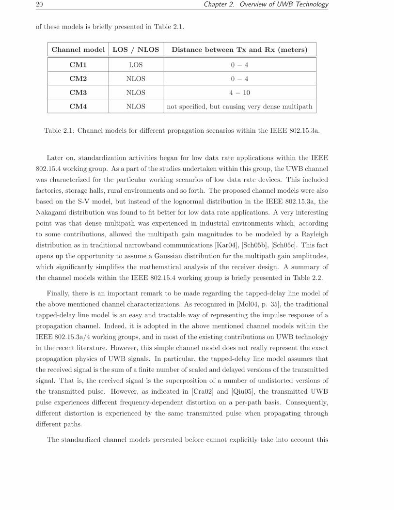
20 Chapter 2. Overview of UWB Technology
of these models is briefly presented in Table 2.1.
Channel model LOS / NLOS Distance between Tx and Rx (meters)
CM1 LOS 0 − 4
CM2 NLOS 0 − 4
CM3 NLOS 4 − 10
CM4 NLOS not specified, but causing very dense multipath
Table 2.1: Channel models for different propagation scenarios within the IEEE 802.15.3a.
Later on, standardization activities began for low data rate applications within the IEEE
802.15.4 working group. As a part of the studies undertaken within this group, the UWB channel
was characterized for the particular working scenarios of low data rate devices. This included
factories, storage halls, rural environments and so forth. The proposed channel models were also
based on the S-V model, but instead of the lognormal distribution in the IEEE 802.15.3a, the
Nakagami distribution was found to fit better for low data rate applications. A very interesting
point was that dense multipath was experienced in industrial environments which, according
to some contributions, allowed the multipath gain magnitudes to be modeled by a Rayleigh
distribution as in traditional narrowband communications [Kar04], [Sch05b], [Sch05c]. This fact
opens up the opportunity to assume a Gaussian distribution for the multipath gain amplitudes,
which significantly simplifies the mathematical analysis of the receiver design. A summary of
the channel models within the IEEE 802.15.4 working group is briefly presented in Table 2.2.
Finally, there is an important remark to be made regarding the tapped-delay line model of
the above mentioned channel characterizations. As recognized in [Mol04, p. 35], the traditional
tapped-delay line model is an easy and tractable way of representing the impulse response of a
propagation channel. Indeed, it is adopted in the above mentioned channel models within the
IEEE 802.15.3a/4 working groups, and in most of the existing contributions on UWB technology
in the recent literature. However, this simple channel model does not really represent the exact
propagation physics of UWB signals. In particular, the tapped-delay line model assumes that
the received signal is the sum of a finite number of scaled and delayed versions of the transmitted
signal. That is, the received signal is the superposition of a number of undistorted versions of
the transmitted pulse. However, as indicated in [Cra02] and [Qiu05], the transmitted UWB
pulse experiences different frequency-dependent distortion on a per-path basis. Consequently,
different distortion is experienced by the same transmitted pulse when propagating through
different paths.
The standardized channel models presented before cannot explicitly take into account this

2.4. Fundamentals of UWB Technology 21
Channel model LOS / NLOS Propagation environment
CM1 LOS Residential
CM2 NLOS Residential
CM3 LOS Office
CM4 NLOS Office
CM5 LOS Outdoor
CM6 NLOS Outdoor
CM7 LOS Industrial
CM8 NLOS Industrial
BAN NLOS† Body-Area-Networks
† Because of the diffraction around the body [For06].
Table 2.2: Channel models for different propagation scenarios within the IEEE 802.15.4.
path-dependent distortion because they are all based on a tapped-delay line model. However,
they do reflect this path-dependent distortion in an implicit manner by introducing phantom
paths [Ben06]. These paths are not real but just an artifact to represent the different pulse
distortion among real paths. Consequently, care must be taken when interpreting the proposed
models. This is because each path in the model does not necessarily represent a separate
independent path in reality, so that the fading coefficients of different delay bins need not be
independent.
As a result of the above considerations, the main conclusion is that the channel model
for UWB signals must be regarded more as a black box than as a real representation of the
propagation physics. Therefore, the proposed channel models are intended to evaluate the
performance of UWB systems in terms of statistical parameters such as delay spread, temporal
correlation, etc. rather than in terms of detailed temporal characteristics such as, for instance,
the required number of fingers in a Rake receiver.
2.4.4 Pulse distortion
Pulse distortion is certainly the major reason of this dissertation. Contrary to traditional nar-
rowband communication systems, pulse distortion is one of the unique characteristics of UWB
systems and it requires a completely different approach for the receiver design. Consequently,
new opportunities arise for developing a theoretical framework in which one of the key elements
is the lack of knowledge about the received wave shape.

22 Chapter 2. Overview of UWB Technology
Pulse distortion has been under investigation since the early 1900s in the context of diffraction
at a half-plane for sound pulses [Som01], [Lam10]. Later on, military investigations were carried
out for transient wave pulses originated from nuclear detonations. However, it was not until
the 1990s that initial studies for the pulse distortion of UWB signals started to be developed
[Sch93]. Up to now, there are many important contributions on this topic. In particular, special
emphasis should be given to the work by R. C. Qiu, one of the major contributors to the
pulse distortion theory of UWB signals [Qiu95], [Qiu96], [Qiu02], [Qiu04], [Qiu05]. The work
by Qiu is based on the geometric and the uniform theories of diffraction (GTD/UTD), which
can be viewed as an asymptotic theory (i.e. frequency f → ∞) of the solution to Maxwell’s
equations. As a result of the studies by Qiu, a clear conclusion can be drawn. For the case
of UWB channels, diffraction and dispersion leads to different frequency-dependent distortion
for each echo. In that sense, exact and approximate formulations based on GTD/UTD allow
a modification of the classical tapped-delay line model such that the impulsive response in a
multipath environment can be expressed as the sum of differently distorted, scaled and delayed
pulses (for details, see [Ben06, Section 2.3]). However this is still a rather complex model and
the state of the art in approximating per-path impulse responses is very primitive. For this
reason the modeling of the per-path distortion is usually combined in a statistical manner with
the traditional tapped-delay line. This is the case, for instance, of the phantom paths already
mentioned in Section 2.4.3.
Apart from diffraction and reflection, the radiating antenna is another important cause
of pulse distortion. Basically, this is due to frequency-dependent variations in the antenna
impedance and radiation pattern [Kon05]. As a result of the impedance variation, the spectrum
of the radiated signal is modified and signal distortion is experienced. In turn, the radiation
pattern variation causes radiation at a given frequency to be concentrated on a certain part of
the antenna. This causes the antenna frequency response to vary for different angles in both
elevation and azimuth. An important point to be highlighted is that, since the pulse shape
produced by the antenna is different for different angles, the notion of a single pulse shape
channel modeling is again problematic. Detailed measurements on this topic have been carried
out by [Bue04]. Finally, signal distortion is also introduced because different signal frequency
components may travel different distances and thus, all frequency components do not reach the
receiver at the same time [Har04].
In front of this complex scenario where the received pulse shape may vary from different
paths and different angles, a typical approximation in practice is to assume that the line-of-
sight pulse is the transmitted pulse shape. This pulse shape is often adopted for matched filter
correlation or to create the discrete tap impulse response channel when analyzing experimental
data. However, care must be taken when making this assumption. On the one hand, matched
filtering with the incorrect pulse shape leads to a significant loss in correlation energy. On the
other hand, using a single pulse for channel modeling will require the generation of additional

2.5. Applications of UWB Technology 23
multipath components for representing the pulse distortion of actual paths. Clearly, this is a
rather loose approximation, and one of the main objectives of this dissertation is to address the
problem of random and time varying pulse shape in a more rigorous manner.
2.5 Applications of UWB Technology
During the last five decades, the unprecedented large bandwidth of UWB signals has been
mainly exploited for radar and ground penetrating sounding [Tay94]. However, the release of
the DARPA report on UWB technology in 1990 and the FCC R&O in 2002 have attracted
significant research efforts for extending UWB technology to commercial applications. This fact
has also been accelerated when the research community realized that UWB systems could be
almost inexpensively implemented with standard CMOS technology.
As already mentioned in Section 2.3.2, two working groups have been created within the
IEEE for defining new physical layers for next generation wireless personal area networks. This
includes both high and low data rate applications, some of which are indicated below:
• High data rate applications:
– Wireless Personal Area Networks (WPAN) for ad-hoc networking between comput-
ers, peripherals and wearable computing. This includes the next generation wireless
universal serial bus (USB) for which both the UWB Forum and the WiMedia Al-
liance are almost to release the first products. Moreover, UWB technology is being
considered as the universal physical layer to support the next generation of Bluetooth
and IEEE 1394 FireWire [Int04], [Int05a], [Int05b].
– Home and professional media networking (digital cameras, DVDs, digital TV, etc.).
– Fourth generation (4G) wireless systems [Chu05].
– Search and rescue imaging systems. This application is intended for police, fire and
rescue services to locate persons hidden behind a wall or under debris in building
collapses.
– Medical applications such as radar monitoring of physiologic functions. Because of
the extremely time resolution of UWB signals, a low-cost and effective monitoring
of internal organs is possible without the need for direct skin contact. Moreover,
ongoing research projects are being conducted for analyzing the backscattered signal
from UWB pulses to detect cancer [Li05], [Con06].
• Low data rate applications:
– Sensor networks with tracking and positioning capabilities [Gez05].
24 Chapter 2. Overview of UWB Technology
– Identification tags for mobile inventory, personnel and asset tracking.
– Location-aware communication systems, a hybrid of radar and data communications
that uses UWB pulses to precisely track the 2-D and 3-D position of an item as well
as transmitting information about the item to a centralized database system.
– Vehicular radar systems for avoiding front and rear collisions.
– Positioning systems for providing real time indoor and outdoor precision tracking.
Some potential uses include locator beacons for emergency services and precision
navigation capabilities for vehicles, industrial and agricultural equipment.
2.6 Challenges in UWB Technology
The most important challenges in UWB technology can be classified into two major groups. On
the one hand, the very large bandwidth of UWB signals results in serious hardware difficulties
for transmitting, receiving and digitally representing such signals. On the other hand, advanced
signal processing techniques must be devised both at the transmitter and receiver in order to
cope with the unique features of UWB signals. For instance, this includes optimal pulse shaping
for fulfilling the FCC spectral masks, data detection in the presence of pulse distortion and
robust synchronization to handle the extremely high time resolution of UWB signals. In this
section, the most challenging issues of these two groups will be discussed.
2.6.1 Hardware implementation challenges
The very large bandwidth of UWB signals poses many difficulties in the implementation of
practical and low-cost UWB devices. The two major hardware implementation problems are
related with the pulse distortion introduced by the radiating antennas and the performance of
ultra-high speed analog-to-digital converters (ADC).
• Antenna distortion. One of the major challenges in the implementation of UWB sys-
tems is the development of suitable antennas that provide minimum pulse distortion at
the receiver. Antennas for UWB signals require to cover a signal bandwidth on the or-
der of several GHz and current research efforts are being pursued in achieving antenna
impedances and radiation patterns that are constant for such a range of frequencies. In
addition, this must be done by using simple manufacturing procedures, low-cost materials
and small geometrical antenna structures for easy integration into small devices.
Since traditional wideband antennas cannot be adopted for UWB applications, specific
designs for UWB antennas are required. Some UWB antennas have been already proposed
in the existing literature. See for instance the planar antenna proposed in [Yaz04], [Yaz05]

2.6. Challenges in UWB Technology 25
or [Brz06], the low-cost Cobra antenna in [Yin04] or the printed-circuit board (PCB)
antennas proposed in [Low05] and [Gue05]. However, all the above proposals provide a
constant behavior just for a portion of the UWB spectrum specified by the FCC. Further
research is still required to provide a more stable behavior for the whole spectrum.
• Analog-to-digital conversion. Another important challenge in the hardware imple-
mentation of UWB systems is related with the analog-to-digital conversion at the receiver.
Because of the very large bandwidth of UWB signals, a sampling rate on the order of a few
gigasamples per second (Gsps) is required, according to the Nyquist criterion. Certainly,
this is an ultra-high speed requirement for the analog-to-digital converter (ADC) and it
becomes the bottleneck of fully digital implementations of UWB receivers.
Currently, there are several approaches to overcome the ultra-high speed requirements of
ADCs for UWB applications. For instance, some authors propose to reduce the sampling
rate by dividing the whole bandwidth into several sub-bands and adopting a parallel
architecture where each ADC operates with a fraction of the required sampling frequency
[Nam03], [Hoy04]. However, the major drawback of this approach is that there appear
many issues related with mismatches between different sub-bands and it requires extra
complexity for integrating multiple signals.
Another very popular alternative is to reduce the sampling rate down to frame-rate or
symbol-rate. This is done by implementing the matched filter operation in the analog do-
main and then sampling its output at the desired rate (see for instance, [Gez04], [Tan05b],
[Tia02] or [Tia05a], among many other). Unfortunately, there are two major drawbacks
for this popular approach. First, the correlation required in the matched filter operation
must be performed in the analog domain. Consequently, many circuit mismatches and in-
stabilities may be encountered in the analog implementation. Second, the received signal
must be perfectly known for implementing the matched filter, and this is not a realistic
assumption in practical UWB receivers.
Finally, a simple approach is being proposed by some authors based on a single ADC
for digitizing the whole bandwidth of the received UWB signal. This is done by taking
advantage of the tradeoff between sampling rate and number of bits per sample [Wal99].
In this sense, high sampling rates can be achieved by ADCs at the expense of reducing
the number of bits per sample. For instance, high-speed single-bit ADCs are proposed in
[Hoy03] and [Hoy05] to implement fully digital UWB receivers. This single-bit approach
seems reasonable since the noise-like spectrum of UWB signals is similar to the one claimed
in traditional spread-spectrum systems for adopting just one bit for the analog-to-digital
conversion at the receiver. However, there is a significant degradation loss in single-bit
receivers when the input signal has a large dynamic range (e.g. because of the presence
of a strong interfering signal). In that case, more bits per sample are required and the
26 Chapter 2. Overview of UWB Technology
available sampling rate dramatically falls down [Le05].
This last approach based on a single ADC for covering the whole UWB frequency range is
the most flexible and appropriate for a fully digital implementation of the signal processing
techniques at the receiver. Commercial ADCs with sampling rates on the order of 1−3
Gsps are already available. Moreover, the rapid advances in VLSI technology are making
possible the commercial release of ADCs with sampling rates over 20 Gsps in the short-term
[Nos04]. Therefore, the adoption of ultra-high speed ADCs for implementing a fully digital
UWB receiver is now possible, and this will be the approach assumed in this dissertation.
2.6.2 Signal processing challenges
Current challenges in signal processing techniques for UWB systems are related to the accom-
plishment of the severe spectral regulations and how to reliably detect the transmitted informa-
tion in the presence of unknown pulse distortion at the receiver. Some of the ongoing research
efforts are briefly summarized herein.
• Optimal pulse shaping. The carrierless nature of original UWB signals is a key feature
that allows simple and low-cost hardware implementation. However, this comes at the
expense of limiting the emissions in order to avoid any possible harmful interference with
existing wireless services. To this end, spectral regulations have been issued and the result
is a set of spectral masks that any UWB device must accomplish for safe operation with
neighboring narrowband equipments.
Spontaneously generated UWB pulses do not in general accomplish the required spectral
masks unless some kind of pre-processing is applied. As a result, it turns out that optimal
pulse shapes for UWB signals must be carefully designed to achieve two basic objectives.
First, to accomplish the required spectral masks. Second, to maximize the signal-to-noise
ratio at the receiver. To this end, several proposals can be found in the literature. For
instance, pulses satisfying the FCC spectral mask are presented in [Par03]. However,
these proposed pulses do not optimally exploit the allowable bandwidth and transmit
power. Another alternative is the adoption of orthogonal pulses as proposed in [Wu04]
which satisfy the FCC spectral mask and allow multiple sub-band allocation.
• Channel estimation. The unique features of UWB signals make channel estimation to
significantly differ from the approaches adopted in traditional narrowband and/or spread
spectrum communication systems.
On the one hand, most of the known channel estimation techniques for narrowband com-
munications are based on deterministic properties of cyclostationary modulations (see for
instance, [Liu94], [Ton94], [Hua96b], [Mou95], [Lou00]). As a result, high signal-to-noise

2.6. Challenges in UWB Technology 27
ratios are required for these techniques to succeed. However, the very low-power of UWB
signals results in a very low signal-to-noise ratio (SNR) at the receiver. Thus, specific
channel estimation techniques are required for UWB signals by taking into consideration
the very low SNR of practical UWB working scenarios.
On the other hand, traditional channel estimation techniques focus on the estimation of the
impulse response of the propagation channel. For the case of UWB signals, this may involve
hundreds of delays and amplitudes to be estimated requiring an incredible sampling rate for
resolving independent multipaths. Some contributions based on this approach can be found
in the literature, for instance, the iterative method proposed in [Lot00]. However, it is
always recommended to avoid such a huge computational complexity. To this end, research
efforts in channel estimation for UWB systems should be directed toward the estimation
of the aggregate channel response given by the transmitted pulse and the propagation
channel itself. This is an unstructured approach in which the paths of the propagation
channel are completely disregarded and the received waveform is just considered as a whole
[Car03]. In addition, a closed-form solution is also appreciated to avoid iterative solutions
that may require high computational complexity and may suffer from divergence issues in
the presence of low-SNR abnormals. A solution to these issues is proposed in Chapter 4.
• Timing synchronization. Timing synchronization has received significant attention in
the last decades in the context of narrowband carrier-based linear modulations [Gar88],
[Men97], [Vaz00]. However, the carrierless nature of UWB signals, their very low duty
cycle operation, and the pulse distortion caused by the propagation channel and radiating
elements, they all make the timing synchronization a completely different problem for the
case of UWB systems. In addition to this, UWB systems employ extremely-short pulses
with very low-power. Consequently, timing requirements are stringent because even minor
timing misalignments result in lack of energy capture which may render symbol detection
impossible [Tia05b], [Tia05c].
The most challenging issue in the timing synchronization of UWB signals is concerned
with the pulse distortion of the received signal. The reason is that the unknown shape
of the received pulses prevents the implementation of traditional correlation-based timing
detectors. Some methods have been proposed in the recent literature to cope with this
problem. For instance, data-aided techniques for the timing recovery of UWB signals
have been proposed in [Tia05d], [Tia05e] based on the generalized likelihood ratio test. In
[Yan03b], a data-aided technique is also proposed to recover the timing error by correlation
with successive pieces of received signal and data-aided joint timing and channel estimation
is proposed in [Car06b].
Although data-aided techniques provide the best possible performance, a significant draw-
back is that they require some kind of pre-alignment to match the incoming data with the

28 Chapter 2. Overview of UWB Technology
local replica of the training sequence. Therefore, some kind of prior pre-synchronization
is required and this involves extra complexity to the system design. In order to avoid
this problem, nondata-aided techniques for the timing recovery of UWB signals are be-
ing pursued. The advantage is that no prior pre-alignment is required and thus timing
synchronization can be switched on at any time. Moreover, since no training sequence
is transmitted, the effective throughput is maximized and the mean transmitted power is
minimized.
Many nondata-aided timing recovery techniques have been proposed in the literature based
on the concept of dirty template [Yan04a], [Yan05]. The idea behind dirty templates is
to use part of the received signal as the correlation template. This is similar to the
transmitted-reference (TR) approach where an unmodulated pulse is transmitted prior
to each modulated pulse. In that way, the receiver can always take the unmodulated
pulse as the reference pulse for correlation [Rus64], [Hoc02], [Cha03]. However, the major
drawback of timing recovery based on dirty templates is that a relatively high-SNR is
required. Therefore, optimal nondata-aided timing recovery for low-SNR scenarios is still
a pending issue in the timing synchronization of UWB signals. This problem will be
addressed in Chapter 6.
• Data detection in the absence of CSI. Because of the unknown pulse distortion
at the receiver, reliable data detection for UWB systems becomes a challenging task.
When no channel state information is available at the receiver, noncoherent receivers are
the simplest and most cost-effective alternative to the much more complex approach of
estimating the channel and then implementing a coherent receiver. Noncoherent receivers
for UWB signals have been proposed in [Yan04c] and [Yan06], again, based on the concept
of dirty template, and in [Car06a] for the case of orthogonal PPM modulation. However,
further research is still required to determine the optimal data detection strategy. Two
major issues are of special interest. First, the case in which there is waveform overlapping
because of the excessive delay spread of the multipath channel. Second, the case in which
the received waveform exhibits random time variations because of the path-dependent
distortion introduced by relative movements between transmitter and receiver or by moving
objects in-between. These issues will be addressed in Chapter 5.
Chapter 3
Performance Limits of Coherent and
Non-coherent Ultra-Wideband
Communications
3.1 Introduction
In this chapter, the asymptotic performance of UWB communication systems is analyzed from
an information theoretic point of view. To this end, the conditions for which an arbitrarily small
error probability can be achieved are evaluated, and the emphasis is placed on both coherent
and non-coherent receivers operating over multipath fading channels.
On the one hand, coherent receivers are optimal in the sense that they exploit the perfect
knowledge of the end-to-end channel response. This channel state information is usually ob-
tained by using some kind of channel estimation technique prior to the symbol detection stage.
With proper channel knowledge, coherent receivers consist of a traditional correlator-based ar-
chitecture where a replica of the transmitted pulse is used to implement a matched filtering
or Rake receiver [Win98], [Zha03]. On the other hand, non-coherent receivers do not perform
channel estimation and thus, they can be seen as a low-cost and low-power alternative to the
more complex and computationally demanding coherent receivers [Car06a]. The save in hard-
ware complexity is especially important because channel estimation is usually found to require
about 60 % of the total number of gates in the hardware implementation of an UWB coherent
receiver [Yan04b].
A fair decision on whether to use coherent or non-coherent receivers is a question that
basically depends on the signal-to-noise ratio, the transmitted bandwidth and the modulation
format. The interplay between these parameters will be analyzed in this chapter and some
29

30 Chapter 3. Performance Limits of UWB Communications
performance metrics will be provided to shed light on the decision to be made.
The structure of this chapter is the following. The mostly adopted modulation formats
for UWB communication systems are first presented in Section 3.2. This is an important topic
because the ultimate performance of any communication system directly depends on the way the
information is conveyed by the transmitted signal. Next, Section 3.3 reviews some information
theoretic aspects related to the channel capacity and the achievable data rates in the wideband
regime. Note that the wideband regime is of interest for the case under study due to the very
large spectral occupancy of UWB signals. The limits for reliable communication are presented
in Sections 3.4 and 3.5 for coherent and non-coherent UWB receivers, respectively. Finally, a
comparison between these two approaches is presented in Section 3.6.
3.2 Modulation Formats for UWB Communication Systems
3.2.1 PAM or PPM modulation?
The achievable data rate of any communication system is intimately related to the way the
information is conveyed by the transmitted signal. For this reason, before addressing the per-
formance evaluation of UWB communication systems, it is first mandatory to analyze the most
convenient modulation format for reliable communication with UWB signals.
As already mentioned in Section 2.4, the mostly adopted modulation formats for UWB signals
are pulse-amplitude modulation (PAM) and pulse-position modulation (PPM). PAM modulation
requires perfect channel state information in order to resolve the ambiguity introduced by the
channel in the amplitude of the received signal. In contrast, PPM modulation can be either
adopted in the presence or in the absence of channel state information. That is, PPM modulation
can be adopted by either coherent or non-coherent receivers. This is a very important issue
because non-coherent detection is essential in most realistic UWB systems. This is due to
the severe distortion experienced by transmitted pulses when propagating through the UWB
multipath channel. It is found that the received pulses have very little resemblance with the
transmitted ones [Qiu02], [Qiu05], but most importantly, the pulse distortion is found to be
direction-dependent so that it varies when the receiver looks at the transmit antenna from
different directions [Cra02], [Sch05a]. In addition to this, the very large multipath resolution of
UWB signals makes the computation of fast and accurate channel estimates a challenging and
computationally demanding task. Consequently, the possibility of avoiding channel estimation,
and thus implementing low-complexity and non-coherent detection, is certainly appreciated.
Apart from traditional PPM modulation, there are several variations including multipulse
PPM (MPPM), overlapping PPM (OPPM) and differential PPM (DPPM), among other. Inter-
estingly, they all can be regarded as a constrained version of a more general pulse modulation

3.2. Modulation Formats for UWB Communication Systems 31
method called on-off keying (OOK) modulation. In OOK modulation a single bit is transmitted
per channel use. That is, a pulse is transmitted within the symbol duration for representing ”1”
and no pulse is transmitted for representing ”0”. An important point to be taken into consid-
eration is that, since PPM, MPPM, OPPM and DPPM are each a constrained version of OOK
modulation, the capacity of unconstrained OOK becomes the upper bound on the capacity of
these pulse-position modulation formats. As it is shown in [Ham04], the capacity of PPM is
found to be near that of OOK for the low-SNR regime. Consequently, and for the low-SNR
regime, no other constrained version of OOK modulation (e.g. MPPM, OPPM or DPPM) can
offer a significant improvement over traditional PPM. Since one of the emphases of this work is
to focus on the low-SNR regime, we will not consider MPPM, OPPM nor DPPM hereafter but
only the standard and traditional PPM modulation as a reference benchmark.
In the sequel, only PPM modulation will be considered for analyzing the performance limits
of UWB communication systems. The reason to focus on PPM modulation is that it allows either
coherent or non-coherent reception so that a more general overview of UWB communications
can be obtained. On the contrary, PAM modulation is only of interest when perfect channel
state information is available and thus, the potential interest of PAM in hostile propagation
environments is very limited.
3.2.2 Signal model for PPM modulation
Since the performance analysis of UWB systems will be based on PPM modulation, the signal
model for this modulation format is presented herein. Let us consider the following discrete-time
model for the received signal corresponding to a single transmitted PPM symbol,
y = Hxi + w (3.1)
where y ∈ RNss×1 is the vector of received samples with Nss the number of samples per symbol.
The vector w ∈ RNss×1 incorporates the Gaussian contribution from both the thermal noise and
possible multiple access interference with Cw.= E
[wwT
]. The (P × 1) vector xi corresponds to
the i-th PPM symbol from the PPM codebook X : {x0,x1, . . . ,xP−1}. Only the i-th entry in xi
is active. That is, [xi]i = 1 and [xi]j = 0 for all j 6= i. Thus, a PPM modulator can be understood
as an encoder producing P = 2b codewords of a (2b, b) orthogonal code. The shaping matrix
H ∈ RNss×P incorporates the end-to-end channel response between transmitter and receiver.
The columns of the shaping matrix H are indicated by hi with H = [h0,h1, . . . ,hP−1] and they
contain time-shifted replicas of the end-to-end channel response with the time-shift equal to N∆
samples, as illustrated in Figure 3.1.
From the observation of Figure 3.1, the end-to-end channel response has a maximum length
of Ng samples. Then, by taking into consideration the maximum delay spread of the channel
and the maximum PPM time-shift, a guard interval is introduced in order to avoid intersymbol
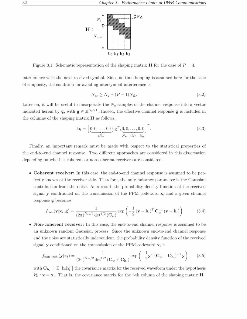
32 Chapter 3. Performance Limits of UWB Communications
Figure 3.1: Schematic representation of the shaping matrix H for the case of P = 4.
interference with the next received symbol. Since no time-hopping is assumed here for the sake
of simplicity, the condition for avoiding intersymbol interference is
Nss ≥ Ng + (P − 1)N∆. (3.2)
Later on, it will be useful to incorporate the Ng samples of the channel response into a vector
indicated herein by g, with g ∈ RNg×1. Indeed, the effective channel response g is included in
the columns of the shaping matrix H as follows,
hi =[0, 0, . . . , 0, 0︸ ︷︷ ︸
iN∆
,gT , 0, 0, . . . , 0, 0︸ ︷︷ ︸Nss−iN∆−Ng
]T. (3.3)
Finally, an important remark must be made with respect to the statistical properties of
the end-to-end channel response. Two different approaches are considered in this dissertation
depending on whether coherent or non-coherent receivers are considered.
• Coherent receiver: In this case, the end-to-end channel response is assumed to be per-
fectly known at the receiver side. Therefore, the only nuisance parameter is the Gaussian
contribution from the noise. As a result, the probability density function of the received
signal y conditioned on the transmission of the PPM codeword xi and a given channel
response g becomes
fcoh (y|xi,g) =1
(2π)Nss/2 det1/2 (Cw)exp
(−1
2(y − hi)
T C−1w (y − hi)
). (3.4)
• Non-coherent receiver: In this case, the end-to-end channel response is assumed to be
an unknown random Gaussian process. Since the unknown end-to-end channel response
and the noise are statistically independent, the probability density function of the received
signal y conditioned on the transmission of the PPM codeword xi is
fnon−coh (y|xi) =1
(2π)Nss/2 det1/2 (Cw + Chi)exp
(−1
2yT (Cw + Chi
)−1 y
)(3.5)
with Chi
.= E
[hih
Ti
]the covariance matrix for the received waveform under the hypothesis
Hi : x = xi. That is, the covariance matrix for the i-th column of the shaping matrix H.

3.3. Review of Information Theoretic Results for Wideband Communications 33
In the sequel, the probability density functions presented in (3.4) and (3.5) will be adopted
for obtaining the performance limits of both coherent and non-coherent communication.
3.3 Review of Information Theoretic Results for Wideband
Communications
3.3.1 Power efficiency in the wideband regime
Power efficiency is, without any doubt, the most important issue in the design of communication
systems where power consumption is the limiting factor. An example of these communication
systems can be found in wireless, deep space and sensor networks devices, among other. In
particular, UWB systems can also be incorporated into this group of low power operating de-
vices. The reason for the low power operation of UWB systems is not only power consumption
but also coexistence and interference avoidance with other systems. In this sense, the Federal
Communications Commission restricts the radiation emissions of UWB systems in order to avoid
possible interference with existing wireless services. For instance, the power spectral density of
UWB signals must be smaller than -41 dBm/Mhz in the [3.1 − 10.6] GHz band and smaller than
-75 dBm/Mhz in the GPS band [FCC02].
Related with the above considerations, a topic that will receive significant attention within
this chapter is the interplay between the low signal-to-noise ratio (SNR) regime and the wideband
regime. The relationship can be found in the fact that the limit of zero SNR is equivalent to
the limit of infinite bandwidth, assuming the transmitted power to be constant. The proof is
straightforward from the definition of the signal-to-noise ratio,
SNR.=
PS
PN=
PS
N0W(3.6)
with PS the signal power, PN the noise power, N02 the double-sided noise spectral density and
W the transmitted bandwidth. Then, for constant signal power, the limit of zero signal-to-noise
ratio can be driven by the limit of infinite bandwidth. That is,
limW→∞
SNR = limW→∞
PS
N0W= 0. (3.7)
For this reason, the low-SNR regime and the infinite-bandwidth regime are often used indistin-
guishably in many contributions in the field of information theory [Por05].
Coming back to the power efficiency requirement, it is interesting to note that a measure for
power efficiency can be obtained from the notion of channel capacity. For a given signal-to-noise
ratio, channel capacity indicates the maximum data rate for which reliable communication is
possible, understanding reliable as having an arbitrarily small error probability. Thus, achieving

34 Chapter 3. Performance Limits of UWB Communications
capacity can be understood as the optimal use of the available power resources. In [Sha48], Shan-
non showed that the capacity of an ideal bandlimited additive white Gaussian noise (AWGN)
channel is given by
C = W log2
(1 +
PS
WN0
)(bits/s). (3.8)
For the case of the infinite-bandwidth, i.e. W → ∞, the capacity results in
C∞.= lim
W→∞C =
PS
N0log2 e (bits/s). (3.9)
That is, the channel capacity depends linearly on the signal power PS when operating under
the wideband (i.e. low-SNR) regime. This is an important feature of the wideband or low-SNR
regime, and it is in contrast with the behavior exhibited for limited bandwidth or medium to
high SNR, where the capacity depends much more slowly on the signal power because of the
logarithmic function in (3.8).
An important issue to be taken into consideration is that channel capacity is a theoretical
upper bound on the error-free performance of a communication system. In that sense, two major
remarks should be made. First, the upper bound behavior implies that no reliable communica-
tion is possible for a data rate greater than capacity. Second, capacity is a theoretical bound and
thus, no specific guidelines are provided on how to design capacity achieving communication sys-
tems. However, it is a known result that the AWGN wideband capacity in (3.9) can be achieved
by certain communication systems. For instance, [Gol49] showed that wideband capacity can
be achieved by using PPM modulation with vanishing duty cycle. That is, when the fraction of
time used for transmission tends to zero. Equivalently this means that wideband capacity can
be achieved by using M -ary orthogonal signaling as long as M → ∞ [Tur59]. Consequently,
there is not much to worry about since achieving capacity is found to be a feasible goal.
3.3.2 Asymptotic performance over fading channels
A step forward can be done by considering fading communication channels. Here, a striking
result was noted by [Ken69] in the sense that channel capacity for the AWGN is not affected by
the presence of fading as long as the bandwidth is large enough. That is,
CAWGN∞ = C
fading∞ . (3.10)
The result in (3.10) was also noted by [Gal68] and it was initially conceived for the case of
Rayleigh fading channels. However, an extension was presented by [Tel00] to show that wideband
capacity for the AWGN channel is indeed a rather general result that coincides with wideband
capacity for a general class of fading channel models. In addition, the result in (3.10) assumes
the absence of channel state information at the transmitter, but it holds regardless of whether
channel state information is available at the receiver or not.

3.3. Review of Information Theoretic Results for Wideband Communications 35
The wideband capacity identity in (3.10) has important consequences in our study of coherent
and non-coherent UWB communications. In particular, the result in (3.10) claims that the same
achievable data rates can be achieved in the presence of fading regardless of whether coherent
or non-coherent receivers are adopted. However, this is a rather daring assumption and some
fine analysis will be required in order to determine the conditions for this to occur. In any case,
it is interesting to question ourselves how the wideband capacity can be achieved by practical
communication systems over fading channels. Some answers can be found in [Jac63] and [Pie66],
where the wideband capacity over Rayleigh fading was found to be achieved by using M -ary
orthogonal frequency shift keying (FSK) with vanishing duty cycle and non-coherent detection.
This result was extended by [Luo02] to show that FSK with vanishing duty cycle can achieve
capacity on ultra-wideband channels even with limits on bandwidth and peak power.
Among all the results for capacity achieving communication systems, a common charac-
teristic is the peakiness of the transmitted signals either in time or frequency. This fact is
confirmed in [Ver02b] where a formal proof is presented to show that peaky- or flash-signaling
on-off schemes are required to achieve capacity when there is no channel knowledge at the re-
ceiver. Consequently the impulsive nature of UWB signals seems to be inherently designed to
achieve capacity with non-coherent receivers. However there are some drawbacks associated with
peaky signaling. The optimal input signals for non-coherent receivers are increasingly peaky as
the SNR diminishes and thus, communication systems with some kind of peakiness constraint
(i.e. peak-to-average power) experience a severe degradation in the low-SNR regime. Peaki-
ness constraints and their impact on second and fourth order moments of the input signal are
addressed in [Gur05a]. The results in [Gur05a] show that communication systems with aver-
age power and peak-to-average power constraints require infinite energy per bit in the limit of
infinite bandwidth when no channel state information is available at the receiver.
Unfortunately, the conclusion from the above statement is that practical peaky signaling
schemes are not likely to achieve wideband capacity when peakiness constraints are imposed
due to spectral regulations. Thus, we now see that achieving wideband capacity may not be an
attainable goal for certain communication systems. Even though, a pending issue is to determine
how close the ultimate performance can be to that limit.
3.3.3 Wideband optimality and minimum Eb/N0
Most information theoretic studies for wideband channels are based on extrapolating the results
obtained under the hypothesis of infinite bandwidth. Based on this assumption, the following
statements are usually claimed,
• Wideband capacity is not affected by fading.

36 Chapter 3. Performance Limits of UWB Communications
• Channel state information does not alter wideband capacity.
• On-off signaling is wideband optimal.
However, the above claims suffer from some inaccuracies when ignoring the real effect of finite
bandwidth and peakiness constraints on the behavior of channel capacity. Indeed, little attention
is usually paid to the convergence rate at which wideband capacity is achieved as a function of
bandwidth. In that case, it would be found that on-off signaling is no longer optimal since it
requires six times the minimum bandwidth to achieve capacity [Ver02a]. This example illustrates
the importance of considering the convergence rate of spectral efficiency as a crucial measure
for determining optimality.
In the analysis of capacity, one of the most important parameters to be considered is the
convergence rate as a function of energy-per-bit to noise spectral density, Eb/N0, where
Eb
N0=
W
RSNR =
SNR
RW
(3.11)
with R the data rate in bits/s. In particular, it is found that achieving capacity with infinite
bandwidth is equivalent to achieving minimum Eb/N0. That is,(
Eb
N0
)
min
≡(
Eb
N0
)
|R=C∞
=SNR
C∞
W
= log 2 = −1.59 dB. (3.12)
Consequently, achieving the minimum energy per bit has also been adopted as a synonym of
asymptotic optimality in the wideband regime. Due to the interplay between wideband regime
(i.e. W → ∞) and vanishing SNR (i.e SNR → 0), the minimum energy per bit in (3.12) can also
be expressed as(
Eb
N0
)
min
= limW→∞
SNR
RW
= limSNR→0
SNR
C(SNR)(3.13)
where C(SNR) = RW is now the capacity in bits/s/Hz.
The identity in (3.13) is particularly interesting because it clearly indicates that minimum
energy per bit is defined in the limit of SNR → 0. Since capacity is a positive concave and
monotically decreasing function for decreasing SNR, we have that limSNR→0 C(SNR) = 0. Then,
minimum energy per bit is indeed defined in the limit of C → 0. This is a very subtle aspect now,
but it will become a key issue in the convergence analysis of wideband capacity to be presented
later on.
3.3.4 First and second order analysis of spectral efficiency
The topic of spectral efficiency, that is, the capacity behavior as a function of Eb/N0, is analyzed
in [Ver02b] based on the second order Taylor expansion of the channel capacity,
C(SNR) = C′(0)SNR +
1
2C′′(0)SNR
2 + o(SNR
2)
(3.14)
3.3. Review of Information Theoretic Results for Wideband Communications 37
with C′(0) and C′′(0) the first and the second derivatives of the channel capacity evaluated at
SNR = 0. One of major contributions of [Ver02b] is that it establishes a clear link between
spectral efficiency and the derivatives of the channel capacity in the wideband regime.
• Role of C′(0): The first derivative of channel capacity at SNR = 0, C′(0), is intimately
related with the minimum required bit energy for reliable communication. In particular,
[Ver02b] shows that (Eb
N0
)
min
=1
C′(0). (3.15)
The result in (3.15) can easily be proved by substituting the Taylor expansion (3.14)
into (3.13). For the AWGN and Rayleigh or Rice fading channels with channel state
information, the first derivative results in C′(0) = 1log 2 so that the minimum required
(Eb/N0) for reliable communication becomes the well-known value of (Eb/N0)min = log 2 =
−1.59 dB.
Furthermore, communication systems achieving the limit of (Eb/N0)min are defined as
first order optimal. First order optimality is ensured for coherent receivers and it is also
achieved by non-coherent receivers as long as unconstrained peaky signaling is allowed in
the wideband regime.
• Role of C′′(0): The second derivative of channel capacity at SNR = 0, C′′(0), is related
with the rate of convergence at which (Eb/N0)min is achieved. That is, C′′(0) is related
with the slope of the channel capacity versus Eb/N0 curve at SNR = 0. This slope is
indicated by S0 and it is referred to as the wideband slope. In [Ver02b], the wideband
slope is expressed as
S0 = −2[C′(0)]2
C′′(0)(bits/s/Hz/3 dB) (3.16)
and it is defined as the increase in bits/s/Hz that is experienced when increasing 3 dB in
the energy per bit from (Eb/N0)min.
It is interesting to note that the wideband slope depends crucially on the receiver knowledge
of the channel. For a general class of fading channels, the second derivative C′′(0) is a finite
nonzero value when channel state information is available at the receiver. Consequently,
a finite nonzero value is obtained for the wideband slope of coherent receivers. However,
C′′(0) = −∞ when the channel is unknown to the receiver. Thus, the wideband slope for
non-coherent receivers is found to be S0 = 0 and wideband capacity is achieved much more
slowly than for the coherent case.
Finally, communication systems achieving both the wideband slope and (Eb/N0)min are
defined as second order optimal.

38 Chapter 3. Performance Limits of UWB Communications
From the above considerations, the convergence rate analysis of capacity is intimately related
with channel knowledge at the receiver and peakiness constraints. For the sake of clarity, some
examples of capacity curves with first and second order optimality are depicted in Figure 3.2.
Figure 3.2: Examples of different capacity curves for illustrating the concepts of first and second
order optimality.
A brief presentation of the different working scenarios to be considered is presented in Table
3.1. The most important conclusion to be drawn from this table is that the absence of channel
knowledge (i.e. non-coherent receivers) results in the wideband slope to be S0 = 0. This is in
contrast with AWGN channels (i.e. coherent receivers) where the wideband slope is S0 = 2. As
a result, non-coherent receivers can be seen to be trapped in the region of C → 0 because a large
increase in bit energy is required to achieve the non-null capacity region when departing from
the limit of C → 0. That is, a zero wideband slope indicates that even when the bit energy is
increased in 3 dB, the resulting capacity is still zero. In contrast, a 3 dB increase in bit energy
for coherent receivers results in capacity to move from C = 0 to C = 2 bits/s/Hz, as observed in
Figure 3.3 for the AWGN channel when optimal Gaussian inputs are considered.
Another important remark to be made is the one regarding the infinite minimum bit energy
required by non-coherent receivers under peakiness constraints. As shown in [Gur05b], when the
channel is unknown but no peaky-signaling is allowed because of peak constraints, then C′(0) = 0
and infinite minimum bit energy is required when C → 0. That is, non-coherent receivers
converge much more slowly to the wideband capacity because of the difficulty in escaping from
the C → 0 region. This also means that operating at very low SNR (i.e. SNR → 0 and thus,
C → 0) is power inefficient and the practical (i.e. the effective) minimum bit energy is achieved
for a nonzero value of capacity. This is in contrast with traditional AWGN channels, where
minimum bit energy is always achieved at C = 0.
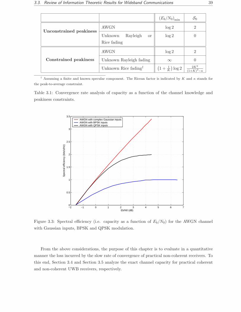
3.3. Review of Information Theoretic Results for Wideband Communications 39
(Eb/N0)min S0
Unconstrained peakinessAWGN log 2 2
Unknown Rayleigh or
Rice fading
log 2 0
Constrained peakiness
AWGN log 2 2
Unknown Rayleigh fading ∞ 0
Unknown Rice fading†(1 + 1
K
)log 2 2K2
(1+K)2−κ
† Assuming a finite and known specular component. The Ricean factor is indicated by K and κ stands for
the peak-to-average constraint.
Table 3.1: Convergence rate analysis of capacity as a function of the channel knowledge and
peakiness constraints.
−2 −1 0 1 2 3 4 5 6 70
0.5
1
1.5
2
2.5
3
3.5
Eb/N0 (dB)
Spe
ctra
l effi
cien
cy (
bits
/s/H
z)
AWGN with complex Gaussian inputsAWGN with BPSK inputsAWGN with QPSK inputs
Figure 3.3: Spectral efficiency (i.e. capacity as a function of Eb/N0) for the AWGN channel
with Gaussian inputs, BPSK and QPSK modulation.
From the above considerations, the purpose of this chapter is to evaluate in a quantitative
manner the loss incurred by the slow rate of convergence of practical non-coherent receivers. To
this end, Section 3.4 and Section 3.5 analyze the exact channel capacity for practical coherent
and non-coherent UWB receivers, respectively.
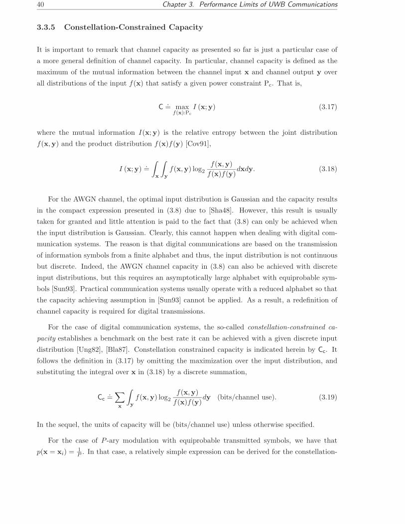
40 Chapter 3. Performance Limits of UWB Communications
3.3.5 Constellation-Constrained Capacity
It is important to remark that channel capacity as presented so far is just a particular case of
a more general definition of channel capacity. In particular, channel capacity is defined as the
maximum of the mutual information between the channel input x and channel output y over
all distributions of the input f(x) that satisfy a given power constraint Pc. That is,
C.= max
f(x):Pc
I (x;y) (3.17)
where the mutual information I(x;y) is the relative entropy between the joint distribution
f(x,y) and the product distribution f(x)f(y) [Cov91],
I (x;y).=
∫
x
∫
y
f(x,y) log2
f(x,y)
f(x)f(y)dxdy. (3.18)
For the AWGN channel, the optimal input distribution is Gaussian and the capacity results
in the compact expression presented in (3.8) due to [Sha48]. However, this result is usually
taken for granted and little attention is paid to the fact that (3.8) can only be achieved when
the input distribution is Gaussian. Clearly, this cannot happen when dealing with digital com-
munication systems. The reason is that digital communications are based on the transmission
of information symbols from a finite alphabet and thus, the input distribution is not continuous
but discrete. Indeed, the AWGN channel capacity in (3.8) can also be achieved with discrete
input distributions, but this requires an asymptotically large alphabet with equiprobable sym-
bols [Sun93]. Practical communication systems usually operate with a reduced alphabet so that
the capacity achieving assumption in [Sun93] cannot be applied. As a result, a redefinition of
channel capacity is required for digital transmissions.
For the case of digital communication systems, the so-called constellation-constrained ca-
pacity establishes a benchmark on the best rate it can be achieved with a given discrete input
distribution [Ung82], [Bla87]. Constellation constrained capacity is indicated herein by Cc. It
follows the definition in (3.17) by omitting the maximization over the input distribution, and
substituting the integral over x in (3.18) by a discrete summation,
Cc
.=
∑
x
∫
y
f(x,y) log2
f(x,y)
f(x)f(y)dy (bits/channel use). (3.19)
In the sequel, the units of capacity will be (bits/channel use) unless otherwise specified.
For the case of P -ary modulation with equiprobable transmitted symbols, we have that
p(x = xi) = 1P . In that case, a relatively simple expression can be derived for the constellation-

3.4. Constellation-Constrained Capacity for Coherent PPM 41
constrained capacity. That is,
Cc =∑
xi
∫
y
f (y|x = xi) p(x = xi) log2
f (y|x = xi)∑xj
f (y|x = xj) p(x = xj)dy (3.20)
=1
P
∑
xi
∫
y
f (y|x = xi) log2
f (y|x = xi)1P
∑xj
f (y|x = xj)dy (3.21)
=1
P
∑
xi
∫
y
f (y|x = xi) log2 Pdy − 1
P
∑
xi
∫
y
f (y|x = xi) log2
∑xj
f (y|x = xj)
f (y|x = xi)dy
= log2 P − 1
P
∑
xi
∫
y
f (y|x = xi) log2
∑xj
f (y|x = xj)
f (y|x = xi)dy (3.22)
so that the constellation-capacity can be expressed as
Cc = log2 P − 1
P
P−1∑
i=0
Ey|xi
log2
P−1∑
j=0
f (y|x = xj)
f (y|x = xi)
. (3.23)
The final result in (3.23) provides a valuable interpretation of the notion of channel capacity. In
particular, note that the argument of the log2(·) operator is indeed a sum of likelihood ratios.
That is, the quotientf(y|x=xj)f(y|x=xi)
in the right hand side of (3.23) is the likelihood ratio for deciding
between the hypothesis Hi : x = xi and the hypothesis Hj : x = xj . Let us indicate the
likelihood ratio by Λj,i(y) as follows,
Λj,i(y).=
f (y|x = xj)
f (y|x = xi). (3.24)
In this way, the constellation-constrained capacity for equiprobable discrete inputs can be ex-
pressed in a more insightful manner as
Cc = log2 P − 1
P
P−1∑
i=0
Ey|xi
log2
P−1∑
j=0
Λj,i(y)
. (3.25)
In the sequel, the constellation-constrained capacity in (3.25) will be evaluated for coherent
and non-coherent UWB receivers. PPM modulation will be adopted since it is widely adopted
in UWB communication systems and it allows for both coherent and non-coherent reception.
Special emphasis will be devoted to spectral efficiency in the wideband regime, where coherent
and non-coherent receivers are expected to exhibit rather different convergence rates.
3.4 Constellation-Constrained Capacity for Coherent PPM
In order to evaluate the constellation-constrained capacity in (3.25), let us first concentrate on
the expression of the likelihood ratio Λj,i defined in (3.24). For the case of coherent communi-
cation, channel state information is available at the receiver. Therefore the input distribution

42 Chapter 3. Performance Limits of UWB Communications
conditioned on a given transmitted symbol xi corresponds to the probability density function
presented in (3.4). With the above considerations, the likelihood ratio Λj,i(y) in (3.25) can be
further manipulated to result in
Λj,i(y,g) =exp
(−1
2 (y − hj)T C−1
w (y − hj))
exp(−1
2 (y − hi)T C−1
w (y − hi)) (3.26)
= exp
(1
2Tr
(C−1
w
[2y (hj − hi)
T + hihTi − hjh
Tj
])). (3.27)
According to the signal model in Section 3.2.2, the likelihood ratio for coherent detection
depends on the particular realization of the end-to-end channel response g within hi, the i-th
column of the channel shaping matrix. The fact is that the channel response is perfectly known
for a given transmission but due to the specific propagation physics of UWB signals, the channel
response may vary from transmission to transmission, and so does the capacity. As a result,
capacity becomes random in the presence of unknown fading variations between consecutive
symbol transmissions. In this situation a meaningful measure for channel capacity must resort
to the expectation of the mutual information I(x;y) over the channel statistics. To this end the
so-called ergodic capacity is defined as
Cc | coh = Eg [I (x;y)] . (3.28)
For the sake of simplicity, the noise contribution is assumed to be white herein. Despite of
the very large bandwidth of UWB signals and the coexistence with many existing narrowband
wireless systems, the white assumption for the noise contribution is commonly adopted in most
of the analysis for UWB communications (see for instance [Ben06] and the references therein).
This assumption is well justified by the low duty cycle of UWB transmissions and the adoption
of time hopping mechanisms for multiple access. In that case,
Cc | coh = (3.29)
log2 P − 1
P
P−1∑
i=0
Eg, y|xi
log2
P−1∑
j=0
exp
(1
2σ2w
Tr(2y (hj − hi)
T + hihTi − hjh
Tj
)) .
In order to further simplify the expression in (3.29), let us substitute the received signal y
by the model y = hi + w. This can be done because the conditioned expectation Ey|xi[·] is to
be performed, and this assumes the transmission of the codeword x = xi and thus the reception

3.4. Constellation-Constrained Capacity for Coherent PPM 43
of the waveform hi. By doing so, we have
Cc | coh = (3.30)
log2 P − 1
P
P−1∑
i=0
Eg, w
log2
P−1∑
j=0
exp
(1
2σ2w
Tr(2 (hi + w) (hj − hi)
T + hihTi − hjh
Tj
))
= log2 P − 1
P
P−1∑
i=0
Eg, w
log2
P−1∑
j=0
exp
( −1
2σ2w
[hT
i hi − 2hTi hj + hT
j hj
])exp
(1
σ2w
(hi − hj)T w
)
= log2 P − 1
P
P−1∑
i=0
Eg, w
log2
P−1∑
j=0
exp
(− 1
2σ2w
‖hi − hj‖2
)exp
(1
σ2w
(hi − hj)T w
) . (3.31)
A closed-form expression for (3.31) is still very difficult to find. One of the main difficulties
is due to the discrete nature of the input alphabet. Discrete input alphabets make the argument
of the log2(·) operator to consist on the sum of likelihood ratios, and this makes difficult to
approximate the nonlinear behavior of the log2(·) with simple linear expansions. The problem
of finding a simple expression for the logarithm of a sum of exponential terms is also a recurrent
problem, for instance, in the field of turbo decoding. In particular, the so-called max-log MAP
algorithm for turbo decoding is based on the approximation log (∑
i exp zi) ≈ maxi xi [Woo00].
However, the max operator is still a nonlinear operator which does not help in providing a
closed-form expression for (3.31).
Since a closed-form expression for (3.31) is still an open problem, Section 3.4.1 provides some
mathematical derivations with the aim of upper bounding the constellation-constrained capacity
in (3.31). To this end, orthogonal signaling is assumed. Once the upper bound is presented, the
goodness of this bound is evaluated by computer simulations.
3.4.1 Closed-form upper bound for orthogonal signaling
Interestingly, a closed-form upper bound for the constellation-constrained capacity in (3.31) can
be obtained when orthogonal PPM signaling is considered. Orthogonal signaling can directly be
obtained by properly designing the transmitted signal such that non-overlapping time intervals
are assigned to different PPM symbols. However, even when some overlapping exists, the ran-
domness of the propagation channel makes the cross-correlation between received waveforms for
different PPM symbols to be almost negligible. That is, the noise-like structure of the received
waveforms contributes to reasonably validate the orthogonal signaling assumption, as confirmed
by the simulation results to be presented later on.
The first important consequence of assuming orthogonal signaling is that the Euclidean
distance in (3.31) turns out to depend on the energy of the received waveform only. That is,
‖hi −hj‖2 = 2Es for i 6= j with Es = ‖g‖2 the energy of the received waveform or, equivalently,
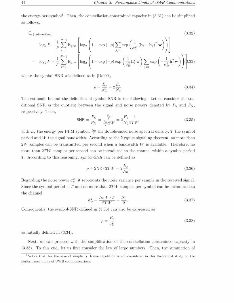
44 Chapter 3. Performance Limits of UWB Communications
the energy-per-symbol1. Then, the constellation-constrained capacity in (3.31) can be simplified
as follows,
Cc | coh+orthog = (3.32)
log2 P − 1
P
P−1∑
i=0
Eg,w
log2
1 + exp (−ρ)
∑
j 6=i
exp
(1
σ2w
(hi − hj)T w
)
= log2 P − 1
P
P−1∑
i=0
Eg,w
log2
1 + exp (−ρ) exp
(1
σ2w
hTi w
) ∑
j 6=i
exp
(− 1
σ2w
hTj w
)
(3.33)
where the symbol-SNR ρ is defined as in [Dol00],
ρ.=
Es
σ2w
= 2Es
N0. (3.34)
The rationale behind the definition of symbol-SNR is the following. Let us consider the tra-
ditional SNR as the quotient between the signal and noise powers denoted by PS and PN ,
respectively. Then,
SNR =PS
PN=
Es
TN02 2W
= 2Es
N0
1
2TW(3.35)
with Es the energy per PPM symbol, N02 the double-sided noise spectral density, T the symbol
period and W the signal bandwidth. According to the Nyquist signaling theorem, no more than
2W samples can be transmitted per second when a bandwidth W is available. Therefore, no
more than 2TW samples per second can be introduced to the channel within a symbol period
T . According to this reasoning, symbol-SNR can be defined as
ρ.= SNR · 2TW = 2
Es
N0. (3.36)
Regarding the noise power σ2w, it represents the noise variance per sample in the received signal.
Since the symbol period is T and no more than 2TW samples per symbol can be introduced to
the channel,
σ2w =
N0W · T2TW
=N0
2. (3.37)
Consequently, the symbol-SNR defined in (3.36) can also be expressed as
ρ =Es
σ2w
(3.38)
as initially defined in (3.34).
Next, we can proceed with the simplification of the constellation-constrained capacity in
(3.33). To this end, let us first consider the law of large numbers. Then, the summation of
1Notice that, for the sake of simplicity, frame repetition is not considered in this theoretical study on the
performance limits of UWB communications.

3.4. Constellation-Constrained Capacity for Coherent PPM 45
exponentials in (3.33) can be assumed to converge to the sum of individual mean values. That
is,∑
j 6=i
exp
(− 1
σ2w
hTj w
)→ (P − 1)Ew
[exp
(− 1
σ2w
hTj w
)]. (3.39)
The assumption above can be reasonably adopted provided that P is sufficiently large and
taking into consideration that the product hTj w does not vary significantly for different j =
{0, 1, . . . , P − 1}. Moreover, the reason for the expectation in the right hand side of (3.39) to be
carried out over the noise w is the following. The length of waveform g within hj is usually very
short compared to the total length of hj . That is, hj is usually sparse. Then, it is reasonable to
assume that moving j makes the short waveform g to correlate with different samples of noise.
Equivalently, the summation in the left hand side of (3.39) is indeed generating different noise
realizations for different values of j.
According to the mathematical derivations in Appendix 3.A, the required expectation is
given by
Ew
[exp
(− 1
σ2w
hTj w
)]= exp
(1
2σ2w
‖hj‖2
)= exp
(1
2ρ
). (3.40)
Note that the result in (3.40) is indeed an exact result. No approximations were made at this
point. Then, by substituting the result in (3.40) into the constellation-constrained capacity in
(3.33) the result is
Cc | coh+orthog ≈ log2 P − 1
P
P−1∑
i=0
Eg,w
[log2
(1 + (P − 1) exp
(−1
2ρ
)exp
(1
σ2w
hTi w
))]. (3.41)
The expression in (3.41) is an approximation of the true constellation-constrained capacity since
the partial result in (3.39) required P to be sufficiently large. Moreover, numerical evaluation
is still required. However, a simple and closed-form expression can be obtained by introducing
the Jensen’s inequality. To this end, let us define the function
g (hi,w).= log2
(1 + (P − 1) exp
(−1
2ρ
)exp
(1
σ2w
hTi w
)). (3.42)
The function g(hi,w) is a convex ∪ function. Consequently, the Jensen’s inequality results in
Ew [g (hi,w)] ≥ g (hi, Ew [w]) = log2
(1 + (P − 1) exp
(−1
2ρ
))(3.43)
because of the zero mean of the Gaussian noise contribution, Ew [w] = 0.
Finally, substitution of the Jensen’s inequality results in the following closed-form upper-
bound for the constellation-constrained capacity of orthogonal PPM signaling with coherent
reception,
Cc | coh+orthog ≤ log2 P − log2
(1 + (P − 1) exp
(−1
2ρ
)). (3.44)

46 Chapter 3. Performance Limits of UWB Communications
3.4.2 Numerical results
In this section, the exact constellation-constrained capacity in (3.31) is evaluated for UWB
signals propagating through the IEEE 802.15.3a and the IEEE 802.15.4a channel models in
[Foe03] and [Mol04], respectively. Since an exact and closed-form expression for (3.31) is very
difficult to be obtained, there is no choice but to evaluate (3.31) in a numerical manner via
Monte-Carlo simulations. These numerical results will be compared with the analytical results
obtained with the closed-form upper bound proposed in (3.44). The advantage of (3.44) is that
it provides a simple and closed-form expression to upper bound capacity. However, (3.44) was
derived assuming orthogonal PPM and thus, it is just a particular case of the more general result
in (3.31).
In order to identify how close we are to the real capacity of orthogonal signaling, and thus,
how valid the proposed upper bound in (3.44) can be, the capacity for coherent orthogonal
signaling is also considered in this study. This expression was derived in [Dol00] and it is
revisited here for the sake of clarity,
Cc | coh+orthog ≈ log2 P − Ev1|x1
[log2 (1 + (P − 1) exp (ρ/2) exp (−√
ρv1))]
(3.45)
with v1 ∼ N(√
ρ, 1). Note that the expression (3.45) derived in [Dol00] requires numerical
evaluation, similarly to what happens with our exact result in (3.31). However, the result in
(3.31) is more general because it encompasses both orthogonal and non-orthogonal coherent
PPM. It is also interesting to point out that the expression in (3.45) was also adopted in [Zha01]
to show the superior performance of UWB PPM systems in comparison with traditional direct-
sequence spread spectrum (DS-SS) for P > 4 in the wideband regime.
Coming back to the simulation results to be presented in this section, the channel models
CM1 and CM2 from the IEEE 802.15.3a working group and the channel model CM8 from the
IEEE802.15.4a working group are considered here. On the one hand, both the CM1 and CM2
channel models assume a distance between transmitter and receiver from 0 to 4 meters. However,
the channel model CM1 considers line-of-sight (LOS) propagation whereas the channel model
CM2 considers non line-of-sight (NLOS) propagation. On the other hand, the CM8 channel
model assumes a distance between transmitter and receiver from 2 to 8 meters with NLOS
propagation in an industrial environment.
The sampling time is set here to Ts = 0.5 ns. The symbol interval is T = 1.5 µs and for
the sake of simplicity, there is only one transmitted pulse per symbol. That is, there is no pulse
repetition within the symbol interval. The PPM time-shift is equal to T∆ = 15 ns. The delay
spread is approximately 25 ns for the CM1 channel model, 50 ns for the CM2 channel model and
100 ns for the CM8 channel model. Since the PPM time-shift is just 15 ns, there is overlapping
between the received waveforms for adjacent hypothesis.
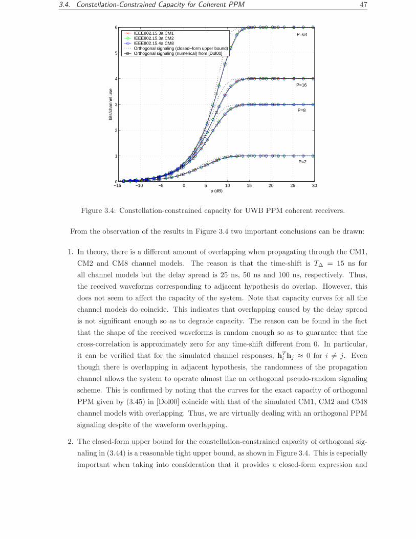
3.4. Constellation-Constrained Capacity for Coherent PPM 47
−15 −10 −5 0 5 10 15 20 25 300
1
2
3
4
5
6
ρ (dB)
bits
/cha
nnel
use
IEEE802.15.3a CM1IEEE802.15.3a CM2IEEE802.15.4a CM8Orthogonal signaling (closed−form upper bound)Orthogonal signaling (numerical) from [Dol00]
P=64
P=16
P=8
P=2
Figure 3.4: Constellation-constrained capacity for UWB PPM coherent receivers.
From the observation of the results in Figure 3.4 two important conclusions can be drawn:
1. In theory, there is a different amount of overlapping when propagating through the CM1,
CM2 and CM8 channel models. The reason is that the time-shift is T∆ = 15 ns for
all channel models but the delay spread is 25 ns, 50 ns and 100 ns, respectively. Thus,
the received waveforms corresponding to adjacent hypothesis do overlap. However, this
does not seem to affect the capacity of the system. Note that capacity curves for all the
channel models do coincide. This indicates that overlapping caused by the delay spread
is not significant enough so as to degrade capacity. The reason can be found in the fact
that the shape of the received waveforms is random enough so as to guarantee that the
cross-correlation is approximately zero for any time-shift different from 0. In particular,
it can be verified that for the simulated channel responses, hTi hj ≈ 0 for i 6= j. Even
though there is overlapping in adjacent hypothesis, the randomness of the propagation
channel allows the system to operate almost like an orthogonal pseudo-random signaling
scheme. This is confirmed by noting that the curves for the exact capacity of orthogonal
PPM given by (3.45) in [Dol00] coincide with that of the simulated CM1, CM2 and CM8
channel models with overlapping. Thus, we are virtually dealing with an orthogonal PPM
signaling despite of the waveform overlapping.
2. The closed-form upper bound for the constellation-constrained capacity of orthogonal sig-
naling in (3.44) is a reasonable tight upper bound, as shown in Figure 3.4. This is especially
important when taking into consideration that it provides a closed-form expression and
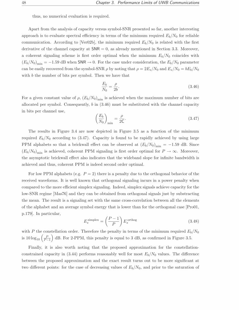
48 Chapter 3. Performance Limits of UWB Communications
thus, no numerical evaluation is required.
Apart from the analysis of capacity versus symbol-SNR presented so far, another interesting
approach is to evaluate spectral efficiency in terms of the minimum required Eb/N0 for reliable
communication. According to [Ver02b], the minimum required Eb/N0 is related with the first
derivative of the channel capacity at SNR = 0, as already mentioned in Section 3.3. Moreover,
a coherent signaling scheme is first order optimal when the minimum Eb/N0 coincides with
(Eb/N0)min = −1.59 dB when SNR → 0. For the case under consideration, the Eb/N0 parameter
can be easily recovered from the symbol-SNR ρ by noting that ρ = 2Es/N0 and Es/N0 = bEb/N0
with b the number of bits per symbol. Then we have that
Eb
N0=
ρ
2b. (3.46)
For a given constant value of ρ, (Eb/N0)min is achieved when the maximum number of bits are
allocated per symbol. Consequently, b in (3.46) must be substituted with the channel capacity
in bits per channel use, (Eb
N0
)
min
=ρ
2C. (3.47)
The results in Figure 3.4 are now depicted in Figure 3.5 as a function of the minimum
required Eb/N0 according to (3.47). Capacity is found to be rapidly achieved by using large
PPM alphabets so that a brickwall effect can be observed at (Eb/N0)min = −1.59 dB. Since
(Eb/N0)min is achieved, coherent PPM signaling is first order optimal for P → ∞. Moreover,
the asymptotic brickwall effect also indicates that the wideband slope for infinite bandwidth is
achieved and thus, coherent PPM is indeed second order optimal.
For low PPM alphabets (e.g. P = 2) there is a penalty due to the orthogonal behavior of the
received waveforms. It is well known that orthogonal signaling incurs in a power penalty when
compared to the more efficient simplex signaling. Indeed, simplex signals achieve capacity for the
low-SNR regime [Mas76] and they can be obtained from orthogonal signals just by substracting
the mean. The result is a signaling set with the same cross-correlation between all the elements
of the alphabet and an average symbol energy that is lower than for the orthogonal case [Pro01,
p.179]. In particular,
E simplexs =
(P − 1
P
)E orthog
s (3.48)
with P the constellation order. Therefore the penalty in terms of the minimum required Eb/N0
is 10 log10
(P
P−1
)dB. For 2-PPM, this penalty is equal to 3 dB, as confirmed in Figure 3.5.
Finally, it is also worth noting that the proposed approximation for the constellation-
constrained capacity in (3.44) performs reasonably well for most Eb/N0 values. The difference
between the proposed approximation and the exact result turns out to be more significant at
two different points: for the case of decreasing values of Eb/N0, and prior to the saturation of
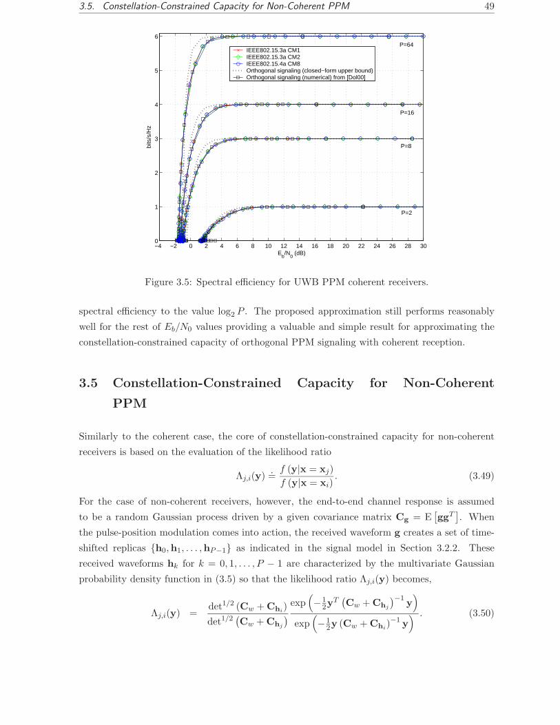
3.5. Constellation-Constrained Capacity for Non-Coherent PPM 49
−4 −2 0 2 4 6 8 10 12 14 16 18 20 22 24 26 28 300
1
2
3
4
5
6
Eb/N
0 (dB)
bits
/s/H
z
IEEE802.15.3a CM1IEEE802.15.3a CM2IEEE802.15.4a CM8Orthogonal signaling (closed−form upper bound)Orthogonal signaling (numerical) from [Dol00]
P=64
P=16
P=8
P=2
Figure 3.5: Spectral efficiency for UWB PPM coherent receivers.
spectral efficiency to the value log2 P . The proposed approximation still performs reasonably
well for the rest of Eb/N0 values providing a valuable and simple result for approximating the
constellation-constrained capacity of orthogonal PPM signaling with coherent reception.
3.5 Constellation-Constrained Capacity for Non-Coherent
PPM
Similarly to the coherent case, the core of constellation-constrained capacity for non-coherent
receivers is based on the evaluation of the likelihood ratio
Λj,i(y).=
f (y|x = xj)
f (y|x = xi). (3.49)
For the case of non-coherent receivers, however, the end-to-end channel response is assumed
to be a random Gaussian process driven by a given covariance matrix Cg = E[ggT
]. When
the pulse-position modulation comes into action, the received waveform g creates a set of time-
shifted replicas {h0,h1, . . . ,hP−1} as indicated in the signal model in Section 3.2.2. These
received waveforms hk for k = 0, 1, . . . , P − 1 are characterized by the multivariate Gaussian
probability density function in (3.5) so that the likelihood ratio Λj,i(y) becomes,
Λj,i(y) =det1/2 (Cw + Chi
)
det1/2(Cw + Chj
)exp
(−1
2yT
(Cw + Chj
)−1y)
exp(−1
2y (Cw + Chi)−1 y
) . (3.50)

50 Chapter 3. Performance Limits of UWB Communications
The expression above can be simplified for the case of AWGN noise, Cw = σ2wI. In this case,
the determinant det (Cw + Chi) in (3.50) turns out to be independent of i and thus
det (Cw + Chi) = det
(Cw + Chj
)(3.51)
for any {i, j}. This statement can easily be proved by noting that σ2wI+Chi
can be understood
as a block partitioned matrix. According to the properties of block partitioned matrices [Har00,
p.185],
det(σ2
wI + Chi
)= det
σ2
wINg + Cg 0
0 σ2wINss−Ng
= det
(σ2
wINg + Cg
)σ
2(Nss−Ng)w .
(3.52)
Since the right hand side of (3.52) does not depend on the time position of the transmitted PPM
symbol, the likelihood ratio simplifies to
Λj,i(y) = exp
(1
2yT
[(σ2
wI + Chi
)−1 −(σ2
wI + Chj
)−1]y
)(3.53)
and constellation-constrained capacity becomes
Cc | no−coh = (3.54)
log2 P − 1
P
P−1∑
i=0
Eg, y|xi
log2
P−1∑
j=0
exp
(1
2yT
[(σ2
wI + Chi
)−1 −(σ2
wI + Chj
)−1]y
) .
It is interesting to note that constellation-constrained capacity for non-coherent receivers in
(3.54) depends on the second-order moments of the received signal. This is in contrast with
the constellation-constrained capacity for coherent receivers in (3.31), where just the first order
moment of the received signal was required. Second-order moments are required for non-coherent
receivers because the absence of channel state information makes the received waveform to be
considered an unknown random Gaussian process with zero-mean. Therefore, the detection
process must resort to second-order statistics in order to distinguish the received signal from
the background noise. The shift from first to second order moments is an important difference
in the constellation-constrained capacity for coherent and non-coherent receivers, and it is the
responsible for the different rate of convergence of spectral efficiency in the wideband regime.
This issue will be discussed in more detail in Section 3.6.
3.5.1 Upper bound for uncorrelated scattering
Similarly to what occurred in Section 3.4 for the case of coherent receivers, the resulting likeli-
hood ratio for non-coherent receivers makes very difficult to obtain a closed-form expression for
capacity in (3.54). In order to circumvent this limitation, a closed-form upper bound will be

3.5. Constellation-Constrained Capacity for Non-Coherent PPM 51
derived herein based on the Jensen’s inequality already applied in Section 3.4.1. By doing so,
the following upper bound is obtained,
Cc | no−coh = (3.55)
log2 P − 1
P
P−1∑
i=0
Eg, y|xi
log2
P−1∑
j=0
exp
(1
2Tr
([(σ2
wI + Chi
)−1 −(σ2
wI + Chj
)−1]yyT
))
≤ log2 P − 1
P
P−1∑
i=0
log2
P−1∑
j=0
exp
(1
2Tr
([(σ2
wI + Chi
)−1 −(σ2
wI + Chj
)−1] (
σ2wI + Chi
)))(3.56)
= log2 P − 1
P
P−1∑
i=0
log2
P−1∑
j=0
exp
(1
2
[Nss − Tr
((σ2
wI + Chj
)−1 (σ2
wI + Chi
))])(3.57)
with yyT the random variable where the Jensen’s inequality is applied. That is,
Eg, y|xi
[Cc | no−coh
(yyT
)]≤ Cc | no−coh
(Eg, y|xi
[yyT
])(3.58)
= Cc | no−coh
(σ2
wI + Chi
). (3.59)
Received waveforms with uncorrelated scattering (US) are obtained when adopting most of
the channel models in the IEEE802.15.3a/4a specifications. In these situations, the covariance
matrices Chifor the received waveforms turn out to be diagonal and significant simplifications
can be done in (3.57). After some straightforward manipulations, the upper bound for the
constellation-constrained capacity of non-coherent receivers with uncorrelated received samples
is given by
C USc | no−coh ≤ log2 P − 1
P
P−1∑
i=0
log2
P−1∑
j=0
exp
(−1
2
Nss−1∑
k=0
γi(k) − γj(k)
σ2w + γj(k)
)(3.60)
with γi(k) = [Chi]k,k the k-th entry of the power delay profile (PDP) of the received waveform
under the hypothesis Hi : x = xi.
3.5.2 Numerical results
In this section, the exact constellation-constrained capacity in (3.54) is evaluated for UWB
signals propagating through the IEEE 802.15.4a channel model CM8 [Mol04]. The reason to
focus on this channel model is that it assumes an industrial environment with NLOS propaga-
tion where the small-scale fading statistics are found to be modeled by the traditional Rayleigh
distribution [Kar04], [Sch05b], [Sch05c]. This is in contrast with the IEEE 802.15.3a channel
models, where the small-scale fading statistics were found to be closer to Nakagami and lognor-
mal distributions, and thus, a rather intricate mathematical treatment is required. For the case
of the Rayleigh distribution encountered in the IEEE 802.15.4a CM8 channel model, a simple
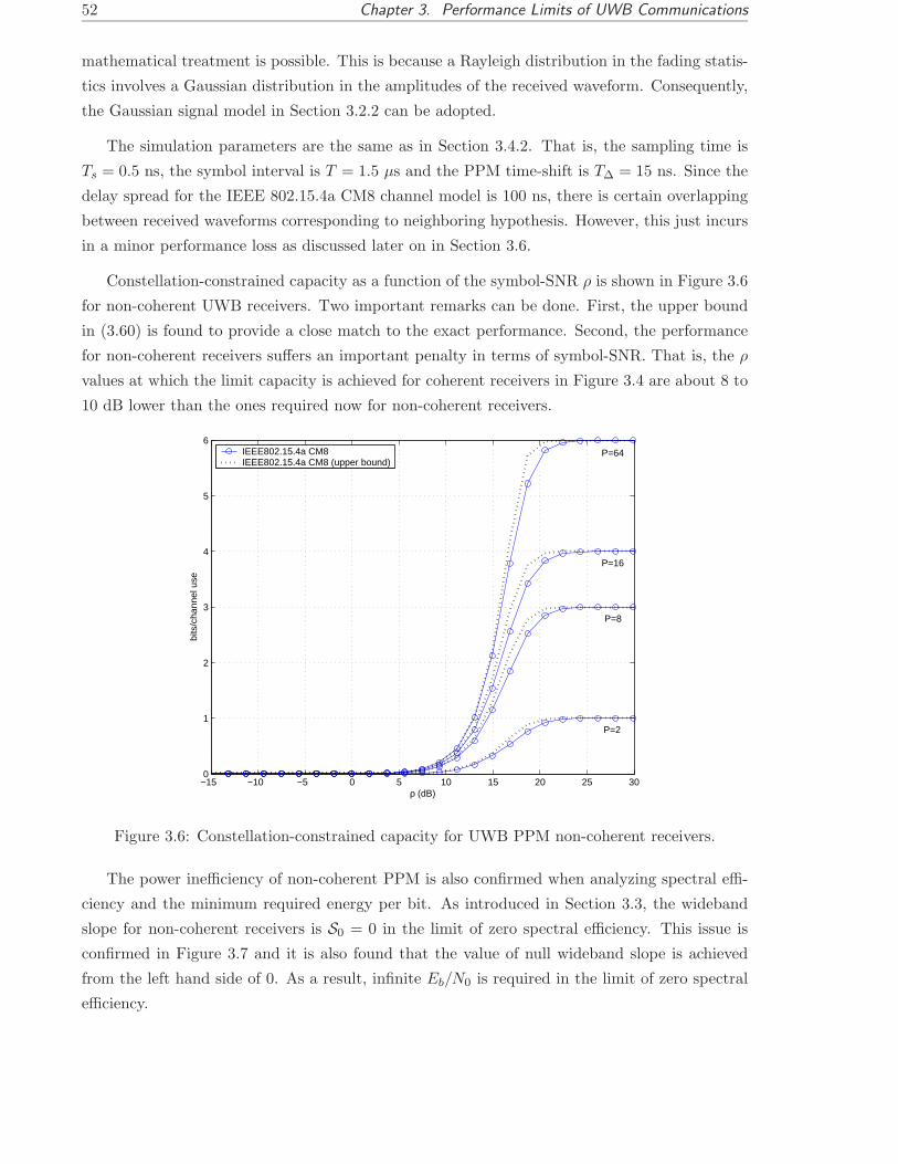
52 Chapter 3. Performance Limits of UWB Communications
mathematical treatment is possible. This is because a Rayleigh distribution in the fading statis-
tics involves a Gaussian distribution in the amplitudes of the received waveform. Consequently,
the Gaussian signal model in Section 3.2.2 can be adopted.
The simulation parameters are the same as in Section 3.4.2. That is, the sampling time is
Ts = 0.5 ns, the symbol interval is T = 1.5 µs and the PPM time-shift is T∆ = 15 ns. Since the
delay spread for the IEEE 802.15.4a CM8 channel model is 100 ns, there is certain overlapping
between received waveforms corresponding to neighboring hypothesis. However, this just incurs
in a minor performance loss as discussed later on in Section 3.6.
Constellation-constrained capacity as a function of the symbol-SNR ρ is shown in Figure 3.6
for non-coherent UWB receivers. Two important remarks can be done. First, the upper bound
in (3.60) is found to provide a close match to the exact performance. Second, the performance
for non-coherent receivers suffers an important penalty in terms of symbol-SNR. That is, the ρ
values at which the limit capacity is achieved for coherent receivers in Figure 3.4 are about 8 to
10 dB lower than the ones required now for non-coherent receivers.
−15 −10 −5 0 5 10 15 20 25 300
1
2
3
4
5
6
ρ (dB)
bits
/cha
nnel
use
IEEE802.15.4a CM8IEEE802.15.4a CM8 (upper bound)
P=64
P=16
P=8
P=2
Figure 3.6: Constellation-constrained capacity for UWB PPM non-coherent receivers.
The power inefficiency of non-coherent PPM is also confirmed when analyzing spectral effi-
ciency and the minimum required energy per bit. As introduced in Section 3.3, the wideband
slope for non-coherent receivers is S0 = 0 in the limit of zero spectral efficiency. This issue is
confirmed in Figure 3.7 and it is also found that the value of null wideband slope is achieved
from the left hand side of 0. As a result, infinite Eb/N0 is required in the limit of zero spectral
efficiency.

3.6. Comparison of coherent and non-coherent performance 53
−5 0 5 10 15 20 25 300
1
2
3
4
5
6
Eb/N
0 (dB)
bits
/s/H
z
IEEE802.15.4a CM8IEEE802.15.4a CM8 (upper bound)
P=64
P=16
P=8
P=2
Figure 3.7: Spectral efficiency for UWB PPM non-coherent receivers.
The power inefficiency of non-coherent receivers is an important result that will receive
further attention in Section 3.6.
3.6 Comparison of coherent and non-coherent performance
The numerical results obtained in Section 3.4 and Section 3.5 will be compared herein for the
case of coherent and non-coherent communication through the IEEE 802.15.4a CM8 channel
model. The comparison will be made for three different information theoretic measures:
• Constellation-constrained capacity.
• Spectral efficiency.
• Achievable data rates for a given transmission bandwidth.
First, exact constellation-constrained capacity as a function of symbol-SNR ρ is depicted in
Figure 3.8. For the non-coherent case, capacity is also evaluated for the case of using a PPM
time-shift with T∆ = 75 ns. This value of T∆ for the CM8 channel model avoids the possible
performance loss caused by overlapping of received waveforms. With T∆ = 75 ns almost 96
% of the received energy is captured without overlapping. With this parameter, the results
indicate that there is almost an 8 dB loss in terms of signal-to-noise ratio due to the adoption
of a non-coherent receiver.

54 Chapter 3. Performance Limits of UWB Communications
−15 −10 −5 0 5 10 15 20 25 300
1
2
3
4
5
6
ρ (dB)
bits
/cha
nnel
use
IEEE802.15.4a CM8 (coherent)IEEE802.15.4a CM8 (non−coherent) T∆=15 ns.
IEEE802.15.4a CM8 (non−coherent) T∆=75 ns.
P=64
P=16
P=8
P=2
Figure 3.8: Constellation-constrained capacity for UWB PPM coherent and non-coherent re-
ceivers.
Spectral efficiency, that is, constellation-constrained capacity as a function of Eb/N0, is
depicted in Figure 3.9. From the observation of this figure, two important conclusions can be
drawn.
1. Coherent PPM is second order optimal for increasing constellation P . However, special
care must be taken when analyzing the results for non-coherent PPM. First of all, it should
be noted that no peaky signaling is simulated herein. Thus, the simulated signal can be
understood to be generated in the presence of peakiness constraints. With this remark
in mind, note that the results for the simulated non-coherent PPM achieve second order
optimality. That is, (Eb/N0)min → ∞ and S0 = 0 as indicated in Table 3.1 for the case
of non-coherent receivers with peakiness constraints. However, this notion of second-order
optimality is not practical in the sense that the required minimum Eb/N0 tends to infinity.
For practical purposes, the effective minimum Eb/N0 can be defined as the true minimum
value of Eb/N0. For the results in Fig. 3.9, this effective minimum Eb/N0 is approximately
equal to 8 dB for the case of non-coherent PPM with P = 64, and it is still far away from
the optimal value of (Eb/N0)min = −1.59 dB for the case of non-coherent PPM with
unconstrained peakiness.
2. The difference between (Eb/N0)min for coherent and non-coherent PPM is on the order of
9 to 10 dB for practical constellation orders. This confirms that in the absence of peaky
signaling, non-coherent PPM is power inefficient from the spectral efficiency point of view.
3.6. Comparison of coherent and non-coherent performance 55
−5 0 5 10 15 20 25 300
1
2
3
4
5
6
7
Eb/N
0 (dB)
bits
/s/H
z
IEEE802.15.4a CM8 (coherent)IEEE802.15.4a CM8 (non−coherent) T∆=15 ns.
IEEE802.15.4a CM8 (non−coherent) T∆=75 ns.
P=64
P=16
P=8
P=2
Figure 3.9: Spectral efficiency for UWB PPM coherent and non-coherent receivers.
However, this penalty can be compensated by the very large bandwidth of UWB signals
which still can provide reasonably high data rates for the low-SNR regime, as shown next
in Figure 3.10.
Achievable data rates for coherent and non-coherent UWB receivers are analyzed for the
symbol period T = 1.5 µs considered in previous simulation results. Then, achievable data rates
in (bits/s) are obtained as
Cc(bits/s) =1
T· Cc(bits/channel use) (3.61)
since one channel use or transmission corresponds to one symbol period of T seconds. The
results for the achievable data rates in (bits/s) are depicted in Figure 3.10 for coherent and
non-coherent UWB receivers under the IEEE 802.15.4a channel model CM8. Figure 3.10 also
incorporates the achievable data rates for the infinite-bandwidth regime C∞ presented in (3.9).
The latter capacity is indeed an upper bound on the achievable data rate of practical coherent
and non-coherent receiver.
The main conclusion by observing Figure 3.10 is that coherent PPM with increasing con-
stellation order is optimal in the sense that it achieves the infinite-bandwidth capacity. This
issue was already pointed out in Figure 3.9 where coherent PPM receivers were found to be
second order optimal. For the case of non-coherent PPM receivers, their power inefficiency in
the low-SNR regime creates a significant gap between their achievable data rates and that of
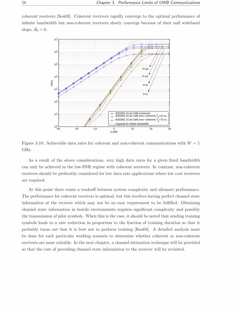
56 Chapter 3. Performance Limits of UWB Communications
coherent receivers [Sou03]. Coherent receivers rapidly converge to the optimal performance of
infinite bandwidth but non-coherent receivers slowly converge because of their null wideband
slope, S0 = 0.
−30 −20 −10 0 10 20 3010
0
101
102
103
104
105
106
107
ρ (dB)
bits
/s
IEEE802.15.4a CM8 (coherent)IEEE802.15.4a CM8 (non−coherent) T∆=15 ns.
IEEE802.15.4a CM8 (non−coherent) T∆=75 ns.
Capacity for infinite bandwidth
P=64
P=16
P=8
P=2
Figure 3.10: Achievable data rates for coherent and non-coherent communications with W = 1
GHz.
As a result of the above considerations, very high data rates for a given fixed bandwidth
can only be achieved in the low-SNR regime with coherent receivers. In contrast, non-coherent
receivers should be preferably considered for low data rate applications where low cost receivers
are required.
At this point there exists a tradeoff between system complexity and ultimate performance.
The performance for coherent receivers is optimal, but this involves having perfect channel state
information at the receiver which may not be an easy requirement to be fulfilled. Obtaining
channel state information in hostile environments requires significant complexity and possibly
the transmission of pilot symbols. When this is the case, it should be noted that sending training
symbols leads to a rate reduction in proportion to the fraction of training duration so that it
probably turns out that it is best not to perform training [Rao04]. A detailed analysis must
be done for each particular working scenario to determine whether coherent or non-coherent
receivers are most suitable. In the next chapter, a channel estimation technique will be provided
so that the cost of providing channel state information to the receiver will be revisited.
3.A Derivation of the expectation on the form Ew
[exp
(βuTw
)]57
Appendix 3.A Derivation of the expectation on the form
Ew
[exp
(βuTw
)]
The purpose of this Appendix is to derive the expectation on the form Ew
[exp
(βuTw
)]with
β a constant scalar, u ∈ RNss×1 a constant vector, and w ∈ R
Nss×1 ∼ N(0, σ2
wI). That is, w is
a zero-mean random Gaussian vector with covariance matrix Ew
[wwT
]= σ2
wI and probability
density function
fw (w) =1
(2πσ2w)Nss/2
exp
(− 1
2σ2w
‖w‖2
). (3.62)
The first step is to expand the expectation operator into its integral form,
Ew
[exp
(βuTw
)]
=
∫
w
exp(βuTw
)fw (w) dw (3.63)
=
∫
w
exp(βuTw
) 1
(2πσ2w)Nss/2
exp
(− 1
2σ2w
‖w‖2
)dw (3.64)
=
∫
w
1
(2πσ2w)Nss/2
Nss−1∏
m=0
exp (β [u]m [w]m) exp
(− 1
2σ2w
[w]2m
)dw (3.65)
=
∫
w
1
(2πσ2w)Nss/2
Nss−1∏
m=0
exp
(− 1
2σ2w
[[w]2m − 2σ2
wβ [u]m [w]m
])dw. (3.66)
Next, it is interesting to complete the quadratic argument of the exponential in (3.66) so as
to make appear the probability density function of a Gaussian distributed vector with some
non-zero mean. To this end note that
exp
(− 1
2σ2w
[[w]2m − 2σ2
wβ [u]m [w]m
])
= exp
(− 1
2σ2w
[[w]2m − 2σ2
wβ [u]m [w]m + σ4wβ2 [u]2m
])exp
(1
2σ2w
σ4wβ2 [u]2m
). (3.67)
Therefore, by substituting (3.67) into (3.66) we have,
Ew
[exp
(βuTw
)](3.68)
=
Nss−1∏
m=0
exp
(σ2
w
2β2 [u]2m
)×
∫
w
1
(2πσ2w)Nss/2
Nss−1∏
m=0
exp
(− 1
2σ2w
[[w]2m − 2σ2
wβ [u]m [w]m + σ4wβ2 [u]2m
])dw
=
Nss−1∏
m=0
exp
(σ2
w
2β2 [u]2m
) ∫
w
1
(2πσ2w)Nss/2
Nss−1∏
m=0
exp
(− 1
2σ2w
([w]m − σ2
wβ [u]m)2
)dw(3.69)
= exp
(σ2
w
2β2‖u‖2
) ∫
w
1
(2πσ2w)Nss/2
exp
(− 1
2σ2w
‖w − σ2wβu‖2
)dw. (3.70)
58 Chapter 3. Performance Limits of UWB Communications
Note that the argument of the integral in (3.70) is indeed the probability density function of a
Gaussian random vector with non-zero mean. Then, since a probability density function is to
be integrated, the result of this integral is found to be equal to 1.
Finally, and with the above considerations, the expectation we are looking for is given by
Ew
[exp
(βuTw
)]= exp
(σ2
w
2β2‖u‖2
). (3.71)

Chapter 4
Waveform Estimation for the
Coherent Detection of UWB Signals
4.1 Introduction
Coherent detection in digital communication systems aims at inferring the presence of a known
deterministic signal and deciding the most probable transmitted message from an a-priori known
set. In the above statement, it is very important to remark that coherent detection assumes
the received signals to be a-priori known at the receiver. As a result, the detection problem
is rather simple and the optimal solution in the presence of white Gaussian noise leads to the
well-known matched filter detector [Kay98, Ch. 4]. Even for the case of correlated Gaussian
noise, the matched filter optimality can be preserved by whitening the received data with the
inverse covariance matrix of the noise.
The popular matched filter detector is based on correlating the incoming data with the ex-
pected and a-priori known signal. For this reason, the matched filter detector is also referred
to as the replica-correlator or the correlator-based receiver. This architecture has been widely
adopted in a vast range of narrowband and spread-spectrum communication systems. For in-
stance, this was the case of the landmark paper by Scholtz [Sch93] where the basis for multiuser
UWB communication systems was established. In [Sch93], a simple correlation architecture was
adopted since the UWB received pulse was assumed to be a-priori known and to be equal to the
pulse radiated by the transmitter.
In practice, however, the UWB received signal hardly ever resembles the original transmitted
pulse. This was already noticed by Scholtz in [Win00], where the received pulses were also
assumed to be known at the receiver but this time they were explicitly recognized to be different
from the transmitted ones. This issue was confirmed in the channel measurements conducted
59
60 Chapter 4. Waveform Estimation for Coherent Detection
by [Cra98a], [Cra98b], [Cra02] and [Cas02a], among many others, where the UWB propagation
channel was found to exhibit a severe frequency-selective behavior with both angle- and path-
dependent distortion. According to these measurement campaigns, the major conclusion is that
coherent detection of UWB signals cannot be implemented by itself unless precise channel state
information is available at the receiver. That is, channel estimation is indispensable for enabling
the coherent detection of UWB signals, and this constitutes the main motivation of this Chapter.
Channel estimation techniques for UWB signals usually adopt a tapped-delay line model for
representing the impulse response of the propagation channel. As a result, the received signal is
modeled by a set of replicas of a single distorted pulse with different time delays and different
amplitude values. However, it is important to note that this is a rather simplified and not realistic
model. The reason is that a tapped-delay line model assumes that the same pulse is replicated
in time. Therefore, it does not take into account the path-dependent distortion observed in
experimental measurements with UWB signals. Nevertheless, this simplified approach has been
widely adopted in the literature and many contributions have been proposed in this direction.
See for instance [Win97], [Cas02b], [She03] or [Mie03]. The above references are all based on
the Rake receiver, that is, the extension of the matched filter principle for the case of multiple
and resolvable replicas of a deterministic signal [Pri58], [Pro94, p. 840]. The Rake architecture
is composed by a bank of correlators with different time delays for capturing the energy of
the known signal over different propagation paths. Finally, all the correlation outputs are
conveniently weighted before symbol decision.
When adopting the traditional Rake approach for the coherent detection of UWB signals,
another major drawback is that the assumed tapped-delay line model may require hundreds of
delays and amplitudes to be estimated. This involves an incredible computational and hardware
complexity for resolving such a huge amount of paths and for implementing the corresponding
correlators. For this reason, several approaches have emerged to reduce this computational
burden. Most authors propose to reduce the total number of paths to just a small set that
includes the most dominant ones. For instance, the contribution in [Car04b] proposes to localize
clusters of received pulses in order to reduce the search time for finding the most dominant
paths. Similarly, [Ara03] proposes a method for choosing the most dominant paths by taking
into consideration the distortion of the received pulse.
Without resorting to the traditional Rake architecture, the main goal of this chapter is to
solve the two major problems encountered in channel estimation for UWB receivers.
• First, a simple receiver architecture is envisaged where the aggregated channel response,
and not the individual paths and amplitudes, is estimated. This constitutes an unstruc-
tured approach where the paths of the propagation channel are completely disregarded and
the received waveform for a single transmitted pulse is considered as a whole. As a result,

4.2. Signal Model 61
it must be remarked that the focus is placed on the waveform estimation problem instead
of the traditional channel estimation problem. That is, the whole received waveform is
now the parameter of interest. By doing so a single correlator is required at the receiver.
Moreover the intricate path-dependent pulse distortions are inherently incorporated in
the estimated waveform and thus, a more realistic representation of the real propagation
conditions is achieved.
• Second, special attention is devoted to the very low-SNR working conditions of UWB
signals. To this end the low-SNR formulation is adopted herein as an optimizing criterion
exhibiting a robust behavior in front of the noise [Vaz00]. This is an important issue since
most of the existing channel estimation techniques require a medium- to high-SNR to
operate. For instance, about 20 to 30 dB are required in many popular channel estimation
techniques such as the ones in [Ton94], [Mou95] or [Xu95]. Consequently, their application
in the context of UWB communications is doubtful.
Finally, a nondata-aided approach is adopted which avoids the insertion of training symbols.
As a result, the effective throughput is maximized, the mean transmitted power is minimized,
and hardware complexity is reduced since no pre-alignment with the incoming signal is required.
Based on the above considerations, the structure of this chapter is the following. The signal
model for the waveform estimation problem is introduced in Section 4.2. Different modulation
formats are considered in a general signal model that it is not intended to be exclusively restricted
to UWB systems. As a result, the proposed waveform estimator is derived in a general manner
such that it can also be applied to traditional carrier-based narrowband systems. Next, the
waveform estimation framework is presented in Section 4.3 where the unconditional maximum
likelihood approach is considered. Based on the low-SNR approximation, an optimal waveform
estimation technique is proposed in Section 4.4 allowing for both closed-form and iterative
implementations. Finally, simulation results are discussed in Section 4.5 and conclusions are
drawn in Section 4.6.
4.2 Signal Model
The signal model to be considered in this chapter encompasses different modulation schemes
such as pulse-amplitude modulation (PAM), pulse-position modulation (PPM) and amplitude-
pulse-position modulation (APPM). Both the families of PAM and A/PPM modulations can
be jointly considered because PPM can always be expressed as a sum of parallel independent
PAM signals [Mar00]. As a result, the waveform estimation framework for PAM modulation can
easily be extended to cover PPM and APPM modulations in a simple manner, and vice versa.
It is important to remark that the signal model considered in this chapter is rather general

62 Chapter 4. Waveform Estimation for Coherent Detection
and it is not exclusively intended for UWB systems. That is, the proposed waveform estimation
technique can be applied to a wide range of communication systems other than UWB. The only
requirement is the system to be based on one of the above mentioned modulation formats. In
this way, the waveform estimation framework will be derived herein in a general manner. At the
end, the results will be particularized to the case of interest of UWB receivers and simulation
results will be provided for this case.
4.2.1 General signal model in scalar notation
The signal model is based on a received waveform that suffers from an unknown distortion caused
by the radiating elements and/or the frequency-selective and dispersive behavior of the propa-
gation channel. In discrete-time representation, this end-to-end unknown received waveform is
denoted by g(k), and in general, it is assumed to be a complex-valued waveform1. Furthermore,
the unknown waveform g(k) has a maximum time support of Ng samples with k ∈ [0, Ng − 1],
and for Ng > Nss (e.g. in PAM modulation), Ng is assumed to be an integer multiple of the
number of samples per symbol, Nss. Note that this is a more general condition than the one pre-
viously considered in (3.2). Finally, the unknown received waveform g(k) is assumed to remain
constant over the whole observation interval.
With the above considerations, the discrete-time baseband received signal becomes,
r(k) =+∞∑
n=−∞
sng (k − dnN∆ − nNss) + w (k) (4.1)
where the sequence of amplitude modulating symbols is indicated by sn and the sequence of
pulse-position modulating symbols is indicated by dn. The time resolution of the pulse-position
modulation is N∆ samples and it is assumed that dn = {0, 1, . . . , P − 1}. Finally, w(k) is the
additive white Gaussian noise with zero mean and variance σ2w.
4.2.2 General signal model in matrix notation
Let us consider an observation interval comprising a total of N samples, with N a multiple
value of the number of samples per symbol Nss. Then, the received samples r(k) in (4.1) can be
stacked in an (N × 1) vector r as follows, r.= [r(0), r(1), . . . , r(N − 1)]T . As a result, the signal
model in matrix notation can be expressed as2,
r =P−1∑
p=0
Ap(g)xp + w. (4.2)
1This assumption corresponds to a general working scenario. For the case of carrierless UWB signals, the
received waveform would be assumed to be real-valued.2The output of the communication channel (i.e. the received signal) is denoted by r hereafter. This is in
contrast with Chapter 3, where the notation y was adopted, as usual in information theory.

4.2. Signal Model 63
The signal model in (4.2) represents the general signal model for a set of P parallel and indepen-
dent linearly modulated signals. For the p-th signal, the waveform shaping is achieved through
the (N ×L) matrix Ap(g) whose columns are Nss-samples time-shifted replicas of the unknown
waveform g, with g.= [g(0), g(1), . . . , g(Ng − 1)]T . The parameter L is the number of symbols
within the observation interval of N samples, and it can be decomposed in a symmetric manner
as L = 2K + 1 for some positive integer K. Finally, the transmitted symbols for the p-th linear
modulation are included in the (L×1) vector xp and the noise samples are contained within the
(N × 1) vector w.
The signal model in (4.2) is rather general and it serves to either PAM, PPM or APPM
modulations. On the one hand, and for the case of transmitting a traditional PAM modulation,
the number of parallel independent PAM modulations P must be set to P = 1. As a result, there
is only one vector of transmitted symbols x0 = [s0, s1, . . . , sL−1]T that may represent in general
either ASK, PSK or QAM symbols. By doing so, the traditional linear model r = A(g)x0 + w
is obtained. On the other hand, and for case of transmitting M-ary PPM or APPM modulation,
the number of parallel independent PAM modulations P must be set to P = log2(M). In that
case, let’s assume the transmission of the p-th PPM position during the n-th symbol. Then,
since only one pulse-position can be active for a given transmitted symbol, [xp]i 6= 0 if and only
if i = n. In general, the transmitted symbols xp are assumed to be zero mean, Ex [xp] = 0
for any p, and to have a covariance matrix given by Ex
[xpx
Tq
]= 1
P ILδpq, with In the (n × n)
identity matrix and δij the Kronecker delta. For PPM modulation, the hypothesis of zero mean
symbols implies that polarity randomization codes are adopted. This is consistent with the
common approach in many PPM-based UWB systems, where polarity randomization codes are
introduced to avoid the existence of spectral lines that may violate spectral regulations [Nak03].
Figure 4.1: Structure of the shaping matrix Ap(g) with p = 0 for both time division multiple
access (TDMA) and single-carrier per channel (SCPC) transmissions. Since SCPC involves a
continuous transmission, the observation interval at the receiver is always a time-interval of the
whole transmission record. Consequently, the shaping matrix becomes truncated (right).
Finally, let us concentrate on the structure of the shaping matrix Ap(g) since it plays a major
role in the problem of waveform identification to be addressed herein. Note that the shaping

64 Chapter 4. Waveform Estimation for Coherent Detection
matrix Ap(g) has a particular structure where each column is a Nss-samples time-shifted replica
of the unknown waveform g. That is,
Ap(g).= [a−K,p(g),a−K+1,p(g), . . . ,aK,p(g)] , (4.3)
where the n-th column of Ap(g) is given by
an,p(g).= Kn,pg, (4.4)
with Kn,p an (N ×Ng) Nss-samples shift matrix. The set of time-shift matrices Kn,p is defined
from the product of a square (N × N) Nss-samples shift matrix JNss , an (N × N) N∆-samples
shift matrix JN∆, and an (N × Ng) zero-padding matrix Π as follows,
Kn,p.= Jn
NssJp
N∆Π. (4.5)
The general expression for the set of m-samples shift matrices Jm, for any 0 ≤ m ≤ N − 1, and
for the selection matrix Π is given respectively by
[Jm]i,j =
1 : (j − i) = m
0 : (j − i) 6= m, (4.6)
Π.=
[0T
(N−Ng)/2×Ng, INg ,0
T(N−Ng)/2×Ng
]T. (4.7)
Once the signal model for the time-shifted replication of the unknown waveform g has been
defined, the signal model in (4.2) can alternatively be expressed as,
r =P−1∑
p=0
K∑
n=−K
xn,pKn,pg + w (4.8)
with xn,p the n-th entry in xp. The advantage of the formulation in (4.8) is that it clearly
shows the linear dependence of the unknown waveform g with the received signal r. This linear
relationship through the set of matrices Kn,p will be the basis for the derivation of the proposed
waveform estimation technique.
4.2.3 Receiver architecture
The system architecture to be considered in this chapter is represented in the block diagram of
Figure 4.2. It corresponds to a coherent receiver where the key element to be analyzed is the
nondata-aided waveform estimation module. This module is the central part of the coherent
receiver and it is the responsible for providing the channel or waveform state information to
implement the matched-filtering detection and synchronization
Important attention should be paid to the radiofrequency (RF) front end. This accounts for
the low-noise amplifier (LNA), the antialiasing low-pass filtering (LPF) and analog-to-digital

4.2. Signal Model 65
Figure 4.2: Block diagram of the receiver architecture to be considered in this chapter.
conversion (ADC). These are basic elements in any RF front end, and a detailed analysis is out
of the scope of this dissertation. For the case of UWB receivers, the interested reader may found
valuable the contribution in [Wan05] and the references therein.
The key point in the system architecture of Figure 4.2 is that Nyquist rate sampling is
considered. This requires a significant hardware complexity from the ADC point of view, but
it allows a fully digital implementation of the whole receiver. Reduced sampling rate receivers
have been proposed in the recent literature, but they come at the expense of assuming some
kind of a-priori known template for matched filtering in the analog domain. Then, digital
conversion is done at the output of the analog correlation at one sample per frame or one
sample per symbol. However, when the actual received signal is completely unknown, no realistic
template can be assumed for matched filtering and rate reduction. In such a situation, there are
two main options. First, implement a transmitted reference (TR) scheme where unmodulated
pulses are transmitted to serve as noisy templates at the receiver. Second, adopt a fully digital
implementation with Nyquist rate sampling and formulate the optimal detection problem in the
digital domain. The latter will be the approach to be considered herein.
Fully digital implementations offer significant advantages over analog and mixed ana-
log/digital implementations. The robustness, accuracy and stability of digital signal processing
techniques are important advantages that justify the extra complexity of the required ADC. As
indicated in Section 2.6.1, ADC chipsets with sampling rates on the order of 20 Gsps are about
to be released to the market. These sampling rates are beyond the minimum requirements for
Nyquist rate sampling of UWB signals, and they become a fundamental improvement for the
design and implementation of robust UWB receivers.
On the opposite direction, correlation-based receivers can be implemented when the wave-
form estimate is available. In that case, frame synchronization and decision statistics can be ob-
tained by properly processing of the frame-level matched filter outputs. The tasks of correlation-
based synchronization and symbol detection are quite standard in traditional coherent receivers.
For this reason, these tasks will not be addressed in the present dissertation since significant
information can be found in the literature.
66 Chapter 4. Waveform Estimation for Coherent Detection
4.3 Waveform Estimation Framework
Channel estimation techniques usually adopt either a data-aided (DA) or training-based scheme,
or a nondata-aided (NDA) or blind3 approach. When a data-aided approach is adopted, the re-
ceiver uses the knowledge of the training symbols to estimate the channel. Data-aided strategies
provide the best possible performance, but they require the insertion of training symbols and
the pre-alignment of the receiver with the piece of incoming data where the training symbols
are located. In contrast, when a nondata-aided approach is adopted, the transmitted symbols
are assumed to be unknown at the receiver and channel estimation must rely on the struc-
ture and statistical properties of the received signal. Since no training symbols are inserted,
nondata-aided techniques maximize the effective throughput and they avoid the requirement of
any pre-alignment with the incoming data.
The waveform estimation framework to be developed herein concentrates on the nondata-
aided approach and it is based on the seminal work on channel estimation by Tong, Xu and
Kailath in [Ton91] and [Ton94]. In their contributions, Tong et al. showed that by sampling
at a rate greater than the symbol rate, the received signal becomes cyclostationary and blind
channel estimation is possible from second-order statistics4. Since the advent of second-order
blind channel estimation techniques, several methods have been proposed including subspace
decomposition [Lou00], [Mou95], least-squares [Xu95], iterative methods [Hua96a], [Slo94] or
moment matching techniques [Gia97]. An excellent review of these methods can be found in
[Liu96] and [Ton98], and the analysis of the asymptotic performance and limitations in [Zen97a].
Nevertheless, one the main problems of nondata-aided channel or waveform estimation is
the severe impact of the so-called outliers or abnormals when working under practical SNR
conditions. This is especially dramatic when dealing with UWB signals, since the stringent
emission limits force the receiver to operate near the noise floor. For this reason, the application
of traditional channel or waveform estimation techniques is limited in real systems. Basically,
this is caused by the deterministic approach in the analytical formulation of these methods,
which results in a suboptimal performance in the presence of severe noise.
Because of the high-SNR requirements of existing channel and waveform estimation tech-
niques, the main goal of this section is to provide the mathematical framework for the derivation
of optimal waveform estimators to operate in the low-SNR regime. To this end, the low-SNR
formulation is adopted herein as an optimizing criterion exhibiting a robust behaviour in front
of the noise. Notice that the low-SNR approximation is a classical approach both in estimation
and detection theory, and some representative examples can be found in [Kay93], [Men97] or
3The terms ”nondata-aided” and ”blind” are indistinguishably used in this dissertation and they both refer to
estimation techniques that do not require the insertion of training symbols.4This is one of the reasons for adopting Nyquist rate sampling in digital UWB receivers.

4.3. Waveform Estimation Framework 67
[Vaz00]. However, it is indeed a realistic approach when dealing with UWB systems. Finally, it
is also important to remark that the low-SNR assumption does not necessarily imply that the
SNR must be particularly low to guarantee that the estimator will work. In fact, most low-SNR
techniques still perform quite well for a rather wide range of SNR values.
4.3.1 Low-SNR Unconditional Maximum Likelihood Waveform Estimation
The maximum likelihood (ML) criterion is certainly one of the most popular methods in estima-
tion theory since it provides a systematic way for deriving asymptotically unbiased and efficient
estimators [Kay93]. For the problem under consideration, the ML estimate for the waveform g
is the solution to the maximization problem
gML = arg maxg
Λ (r|g;x) (4.9)
where Λ (r|g;x) is the likelihood function of the received data r conditioned on the unknown
waveform g and the transmitted symbols x.
Clearly, the solution to (4.9) depends on the statistical knowledge of the transmitted sym-
bols x. In the case of data-aided or training-based schemes, this leads to a conventional least
squares error (LS) problem. However, a more complex scenario corresponds to the nondata-aided
estimation problem. In that case, the transmitted symbols are unknown and they become a nui-
sance parameter in the ML formulation. To circumvent this limitation, the so-called stochastic
or unconditional maximum likelihood estimation considers the nuisances as unknown random
parameters with a known statistical distribution [Ott93]. Then, the marginal likelihood function
is evaluated with respect to these unknowns, and the UML estimate becomes
gUML = arg maxg
Λ (r|g) = arg maxg
Ex [Λ (r|g;x)] . (4.10)
In general, the expectation Ex [·] in (4.10) poses insurmountable obstacles or leads to a com-
plicated cost function. Consequently, a closed-form solution is difficult to be obtained and the
maximization problem in (4.10) must be solved in a numerical manner by using either a grid
search or iterative/gradient methods [Gia97], [Hua02], [LS04]. In order to circumvent this lim-
itation, the low-SNR approximation is adopted herein as a strategy to reduce the difficulty in
obtaining a closed-form solution to the optimization problem in (4.10). In the sequel, most of
the mathematical derivations for the low-SNR UML criterion are omitted for clarity reasons.
However, they are all given in Appendix 4.A, 4.B and 4.C. The reader is also referred to [Vaz00]
for a more general presentation about the application of the low-SNR approximation to UML
estimation problems.
For the problem at hand, the likelihood function Λ (r|g;x) is based on the Gaussian noise

68 Chapter 4. Waveform Estimation for Coherent Detection
probability density function as follows,
Λ (r|g;x) = C0 exp
− 1
σ2w
∥∥∥r −P−1∑
p=0
A(g)xp
∥∥∥2
(4.11)
with C0 an irrelevant positive constant. Then, by expanding the quadratic norm in (4.11) and
just taking into consideration those terms which depend on the unknown g, we have
Λ (r|g;x) = C1 exp
(2
σ2w
χ (r;g;x)
), (4.12)
χ (r;g;x).=
P−1∑
p=0
Re[xH
p AHp r
]− 1
2
P−1∑
p=0
P−1∑
q=0
xHq AH
q Apxp, (4.13)
with the constant C1.= C0 exp
(−rHr/σ2
w
). Moreover, note that the dependence of A on g is
omitted for the sake of simplicity.
At this point, the low-SNR approach is considered. Under the low-SNR regime, the approx-
imation 2χ (r;g;x) /σ2w ≪ 1 is reasonable and the Taylor series expansion can be applied to
(4.12). Then, the problem of performing the expectation Ex [Λ (r|g;x)] on the Gaussian noise
probability density function is now converted into the problem of performing the expectation
on a Taylor series expansion.
Proceeding in this way, Appendix 4.A shows that the low-SNR UML cost function is given
by
L′ (r|g) = Tr(M
[R − σ2
wINr
])+
1
2‖M‖2
F (4.14)
with M the (Nr × Nr) matrix given by
M.=
Lp−1∑
p=0
Kr∑
n=−Kr
Kn,pggHKHn,p, (4.15)
where a truncated observation interval of Nr samples is now considered. In (4.15), Kr stands
for the one-sided number of Nss-samples shifted replicas of g contained within the observation
interval of Nr samples. Similarly, Lp stands for the number of N∆-samples shifted replicas of g
contained within the same observation interval of Nr samples. Further details will be provided
later on for the parameters Kr and Lp. Moreover, the matrix Kn,p in (4.15) is the (Nr × Ng)
truncated version of the (N × Ng) matrix Kn,p defined in (4.5). That is, in Matlab notation,
Kn,p.= Kn,p (1 : Nr, :). Finally, R is the (Nr × Nr) synchronous autocorrelation matrix of the
received data defined as
R.= lim
L→∞
1
L
L−1∑
n=0
rnrHn (4.16)
with rn.= [r(nNss), r(nNss + 1), . . . , r(nNss + Nr − 1)]T .

4.3. Waveform Estimation Framework 69
It is important to note that the truncated observation interval of Nr samples in (4.14) is fixed
according to the rule Nr = max {Ng, Nss}. As indicated in Appendix 4.A, the truncation of the
observation interval from N samples to Nr samples provides a more intuitive and comprehensive
interpretation of the waveform identification problem. In addition, significant computational
complexity is saved because the matrices involved in (4.14) do not depend on the length of
the observation interval but just on the fixed values of Ng or Nss. Moreover, by choosing
Nr = max {Ng, Nss} we always guarantee that at least one of the waveform replicas completely
falls within the observation interval of Nr samples (see Fig. 4.1).
Once the low-SNR UML cost function has been introduced in (4.14), two important remarks
must be made. First, note that for the observation interval of Nr samples, the signal subspace is
now the linear space spanned by M. Thus, the first term in (4.14) is projecting the synchronous
autocorrelation matrix of the received signal, R, onto the signal subspace. There is an important
detail in this projection, and it is that the contribution of the noise must be first removed from R
by substracting the noise covariance Cw = σ2wINr , as indicated in (4.14). This implies that the
noise power σ2w must be known at the receiver. However, this is not a problem for most modern
communication systems since the knowledge of the noise power is also required in other stages
of the receiver. For instance, it is required by many synchronization and detection techniques
but also by iterative decoding. For this reason it seems reasonable to assume that the noise
power will be available. Otherwise it can be estimated from the eigendecomposition of R to
be considered in Section 4.3.2. Nevertheless, the projection of R onto the signal subspace is
one of the major features of the resulting low-SNR UML cost function. Note that this is in
contrast with many of the existing blind channel/waveform estimation techniques, which are
usually based on the exploitation of the noise subspace [Mou95], [Xu03a], [Zar05]. However, it
seems more convenient to exploit the signal subspace of the received signal rather than the noise
subspace, especially when working in the low-SNR regime. This is because the signal subspace
presents a more robust behavior in front of the noise and possible ill-conditioning than the noise
subspace. Therefore, a more robust performance is expected by using the signal subspace.
The second important remark is that the low-SNR UML cost function in (4.14) incorporates
in a natural manner a second-order constraint for the waveform estimation problem. This
constraint is given by the term ‖M‖2F , and together with the signal subspace projection, both
can be thought to be the waveform dependent terms of a correlation matching problem. This will
be illustrated in more detail in Section 4.4, where the solution to the low-SNR UML cost function
in (4.14) is found to be given by the solution to a least squares problem on the second-order
statistics of the received signal.

70 Chapter 4. Waveform Estimation for Coherent Detection
4.3.2 Subspace-Compressed Approach to the Waveform Estimation Problem
One of the major drawbacks of ML methods is that a closed-form solution is usually difficult to
be obtained. In addition, and for the problem of channel or waveform identification, the adoption
of ML methods is further complicated by the possible existence of local minima [Ton98]. This
is the case of (4.14), where a nonlinear optimization with respect to g is required. However,
a valuable help is given when the information regarding the signal subspace is available. This
is because the subspace-constraint helps the ML estimator to restrict the solution space to a
neighborhood around the true waveform. Thus, a valid estimate for the unknown channel or
waveform is still possible even when close to unidentifiable [Zen97b].
In this sense the purpose of this section is to present a subspace constraint for the low-
SNR UML cost function presented in (4.14). To this end, let R be the (Nr × Nr) synchronous
autocorrelation matrix defined in (4.16). Thus, it is easy to prove that R is asymptotically given
by
R = M + σ2wINr . (4.17)
Moreover, the synchronous autocorrelation matrix R can be decomposed as
R = UsDsUHs + UnDnU
Hn , (4.18)
where Ds = diag(λ1 + σ2w, . . . , λd + σ2
w) contains the d largest signal-subspace eigenvalues of R,
with λ1 ≥ λ2 ≥ . . . ≥ λd, and the (Nr×d) matrix Us contains the corresponding signal-subspace
eigenvectors. Similarly, Dn = diag(λd+1, λd+2, . . . , λNr) contains the Nr − d noise-subspace
eigenvalues with λd+1 = λd+2 = . . . = λNr = σ2w, and the (Nr × (Nr − d)) matrix Un contains
the corresponding noise-subspace eigenvectors.
From (4.17) and (4.18), the signal subspace of the synchronous autocorrelation matrix R
is the linear space spanned by the columns of M, since range{M
}= range {Us}. Then the
dimension of the signal subspace is given by the number of linearly independent columns in M.
In order to make clear the relationship between the signal subspace dimension and the structure
of the received signal, let us define the following parameters. For the case of PAM modulations,
let Lr.= 2Kr +1, for some positive integer Kr, be the number of replicas with a time-shift of Nss
samples contained within the observation interval of Nr samples. Similarly, and for the case of
PPM and APPM modulations, let Lp be the number of replicas with a time-shift of N∆ samples
contained within the observation interval of Nr samples. Then, the relationship between the
parameters Nr, Ng, Lr, Lp and the signal subspace dimension d, is described in Table 4.1.
From the above considerations, and since range{M
}= range {Us}, the most important
point is that the unknown waveform g must be a linear combination of the signal-subspace
eigenvectors. That is,
g = Usα (4.19)

4.4. Proposed Waveform Estimation Technique 71
Observation interval for computing R: Nr = max {Ng, Nss}
Nr Lr Kr Lp d
if Ng ≤ Nss (with PAM) Nss 1 0 0 Lr
if Ng ≤ Nss (with PPM or APPM) Nss 1 0 P Lp
if Ng > Nss (only occurs in PAM) Ng 2⌈
Ng
Nss
⌉− 1 Lr−1
2 0 Lr
Table 4.1: Relationship between the basic signal model parameters.
for some (d×1) vector α such that αH
α = 1. Note that the vector α contains the coordinates of
the unknown waveform with respect to the basis of signal eigenvectors. Moreover, it is important
to remark that the unknown waveform g is an (Ng ×1) vector whereas the vector of coordinates
α in (4.19) is (d×1). The key point is that by sampling at a rate equal or greater than twice the
symbol rate, the maximum dimension of the signal subspace d is guaranteed to be always smaller
than the maximum finite time support of the unknown waveform, Ng. Thus, by projecting the
received signal onto the signal subspace, the total number of unknowns is reduced from Ng to
just d, for the same amount of received data. This can be seen by noting that for the largest
value of d,
dmax = Lr = 2
⌈Nr
Nss
⌉− 1, (4.20)
with Nr.= max {Ng, Nss}, and thus,
dmax < Ng ⇔ Nss ≥ 2. (4.21)
Since the number of subspace coordinates d is smaller than the number of unknown waveform
samples Ng, there is a gain in the effective SNR and a more robust performance in front of the
noise is obtained.
4.4 Proposed Waveform Estimation Technique
The key element for the derivation of the proposed waveform estimation technique is the adoption
of the vec operator. The vec operator stacks the columns of any (M × N) matrix in the form
of an (MN × 1) vector and it is a useful mathematical tool that allows us to obtain a simple
and insightful solution to the low-SNR UML cost function in (4.14). An extended version of
the vec operator, termed vech operator, may also be useful. The vech operator is especially
devoted to dealing with any (M × M) symmetric matrix and it ignores the elements that are
above the diagonal. Consequently, the vech operator eliminates the redundancy of symmetric
matrices and reduces the overall computational burden. However, for the sake of clarity, only

72 Chapter 4. Waveform Estimation for Coherent Detection
the standard vec operator will be considered henceforth. For more details about the vec and
the vech operator, the reader is referred to [Har00, Ch. 16].
By adopting the vec operator, the low-SNR UML cost function in (4.14) is shown in Appendix
4.C to be given by
L′ (r|g) = αHv QH rv +
1
2α
Hv QHQαv (4.22)
where
rv.= vec
(R − σ2
wINr
), (4.23)
Q.=
Kr∑
n=−Kr
Lp−1∑
p=0
(Kn,pU
∗s
)⊗
(Kn,pUs
), (4.24)
αv.= vec
(αα
H). (4.25)
The expression in (4.22) is the basis for the proposed waveform estimation approach. Note
that by using the vec operator a very simple and insightful expression is obtained. In fact the
expression in (4.22) is a quadratic equation with a quadratic unknown αv, since αv = vec(αα
H)
with α the coordinates of the unknown waveform in the basis of the signal eigenvectors. The
key point is to notice that the optimization of (4.22) is equivalent to the optimization of a least
squares problem. That is,
maxαv
L′ (r|g) = maxαv
{α
Hv QH rv +
1
2α
Hv QHQαv
}= min
αv
‖rv − Qαv‖2. (4.26)
Therefore, the low-SNR UML criterion for the waveform estimation problem is equivalent to a
least squares problem but on the second-order statistics of the received signal. This is because
rv = vec (R) contains the samples of the synchronous autocorrelation of the received signal.
For this reason, the expression for the low-SNR UML cost function can be understood as a
correlation matching (CM) method. Based on heuristic reasonings, CM methods have been
previously proposed in the literature for channel estimation problems. However, solving this
problem involves a nonlinear optimization which usually requires numerical evaluation [Zen97b],
[Ton98], [LS04]. In contrast, the low-SNR UML approach presented in this dissertation results
in a simple CM problem with a closed-form solution.
4.4.1 Closed-form solution
Based on the equivalence between the low-SNR UML criterion and the least squares problem in
(4.26), the optimal solution for this particular correlation matching problem is given by
αv = γ(QHQ
)−1QH rv (4.27)
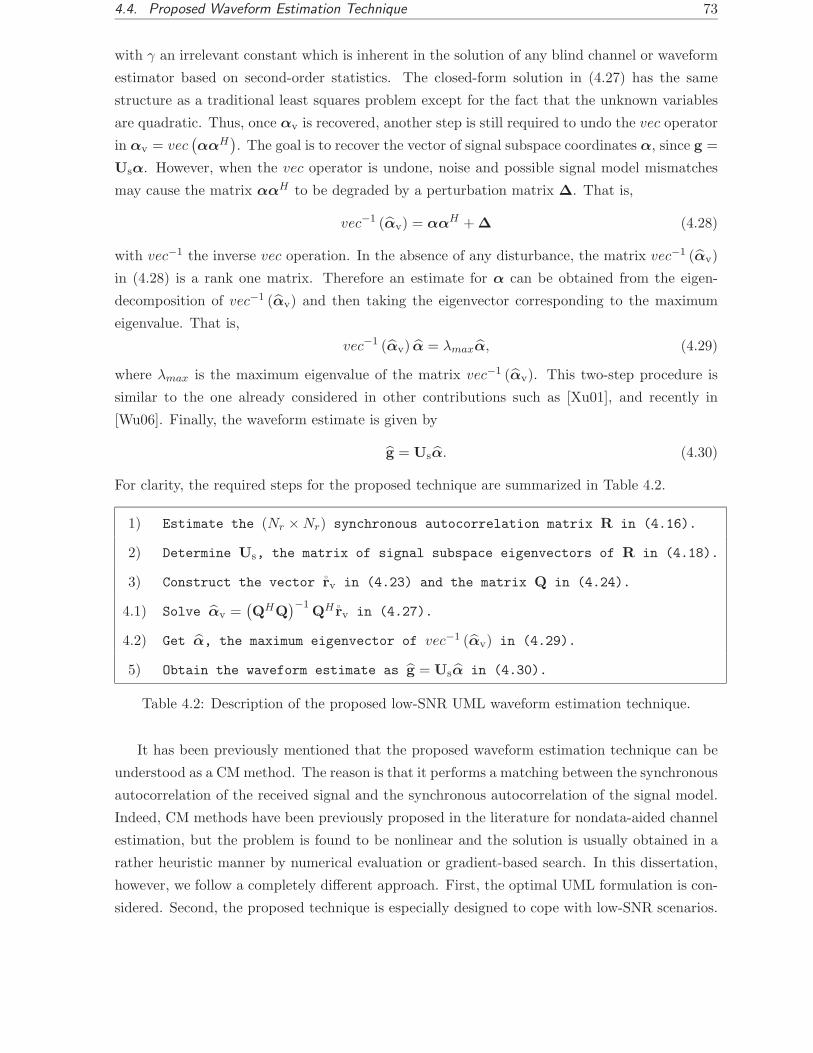
4.4. Proposed Waveform Estimation Technique 73
with γ an irrelevant constant which is inherent in the solution of any blind channel or waveform
estimator based on second-order statistics. The closed-form solution in (4.27) has the same
structure as a traditional least squares problem except for the fact that the unknown variables
are quadratic. Thus, once αv is recovered, another step is still required to undo the vec operator
in αv = vec(αα
H). The goal is to recover the vector of signal subspace coordinates α, since g =
Usα. However, when the vec operator is undone, noise and possible signal model mismatches
may cause the matrix ααH to be degraded by a perturbation matrix ∆. That is,
vec−1 (αv) = ααH + ∆ (4.28)
with vec−1 the inverse vec operation. In the absence of any disturbance, the matrix vec−1 (αv)
in (4.28) is a rank one matrix. Therefore an estimate for α can be obtained from the eigen-
decomposition of vec−1 (αv) and then taking the eigenvector corresponding to the maximum
eigenvalue. That is,
vec−1 (αv) α = λmaxα, (4.29)
where λmax is the maximum eigenvalue of the matrix vec−1 (αv). This two-step procedure is
similar to the one already considered in other contributions such as [Xu01], and recently in
[Wu06]. Finally, the waveform estimate is given by
g = Usα. (4.30)
For clarity, the required steps for the proposed technique are summarized in Table 4.2.
1) Estimate the (Nr × Nr) synchronous autocorrelation matrix R in (4.16).
2) Determine Us, the matrix of signal subspace eigenvectors of R in (4.18).
3) Construct the vector rv in (4.23) and the matrix Q in (4.24).
4.1) Solve αv =(QHQ
)−1QH rv in (4.27).
4.2) Get α, the maximum eigenvector of vec−1 (αv) in (4.29).
5) Obtain the waveform estimate as g = Usα in (4.30).
Table 4.2: Description of the proposed low-SNR UML waveform estimation technique.
It has been previously mentioned that the proposed waveform estimation technique can be
understood as a CM method. The reason is that it performs a matching between the synchronous
autocorrelation of the received signal and the synchronous autocorrelation of the signal model.
Indeed, CM methods have been previously proposed in the literature for nondata-aided channel
estimation, but the problem is found to be nonlinear and the solution is usually obtained in a
rather heuristic manner by numerical evaluation or gradient-based search. In this dissertation,
however, we follow a completely different approach. First, the optimal UML formulation is con-
sidered. Second, the proposed technique is especially designed to cope with low-SNR scenarios.

74 Chapter 4. Waveform Estimation for Coherent Detection
Third, the likelihood function is compressed with the information regarding the signal subspace
instead of using the noise subspace. Fourth, a closed-form solution is provided.
Apart from the above considerations it is also important to remark that, since the proposed
technique can be understood as a CM method, it benefits from the well-known asymptotic
performance of these methods. A detailed analysis on the performance of CM methods was
presented in [Gia97] and [Zen97a]. One of the main contributions was the derivation of a lower
bound for the performance of any CM method, the so-called asymptotic normalized mean square
error (ANMSE), which showed the superior performance of moment-based estimators (e.g. CM
methods) in comparison with traditional eigenstructure-based estimators.
Discussion on the identifiability of the proposed technique
According to the structure of the proposed waveform estimation technique in Table 4.2, the
necessary condition for the waveform g to be uniquely recovered is that the (N2r ×L2
r) matrix Q
in (4.24) must be a full column rank matrix. The reason is that when Q is a full column rank
matrix, there exists a unique solution to the least squares problem J(αv) = ‖rv −Qαv‖2. Once
the solution to αv in (4.27) is found to be unique, then the solution to α, and thus, the solution
to g, are all unique because the relationship between αv, α and g is linear. However, a formal
proof that guarantees the full column rank condition of matrix Q is difficult to be obtained and
it is still under investigation. Meanwhile, it has been heuristically found that the matrix Q is
a full column rank matrix for all the tested waveforms by the authors. This can be seen in
the cumulative results shown in Section 4.5 where the robustness of the proposed technique is
evaluated for randomly generated unknown waveforms.
4.4.2 Gradient-based solution
Apart from the closed-form solution presented in Section 4.4.1, a gradient-based procedure can
also be implemented for obtaining the low-SNR UML estimate for the unknown waveform. At
first glance, there should be no interest in deriving a gradient-based or iterative solution for
the waveform estimation problem since a systematic and straightforward closed-form solution is
available. However, the problem under consideration allows an iterative solution that, in some
circumstances, may provide a slightly better performance than the one provided by the proposed
closed-form implementation.
The reason for the potential performance gain of a gradient-based solution is the avoidance
of the rank one constraint in the recovery of α from the matrix vec−1 (αv) = ααH + ∆ in
(4.28). The matrix vec−1 (αv) is virtually a rank one matrix when ∆ = 0, and thus, with a
single dominant eigenvector. However, noise and possible disturbances result in ∆ 6= 0 which

4.4. Proposed Waveform Estimation Technique 75
may cause the number of significant eigenvectors to be greater than one. In that case recovering
α just by taking the most dominant eigenvector, as proposed in the closed-form implementation
of Section 4.4.1, may introduce certain degradation. In order to circumvent this limitation, and
taking into consideration the properties of the vec operator, a gradient-based solution can be
implemented by using the identity
αv = α∗ ⊗ α (4.31)
and solving the waveform estimation problem for α instead of αv. This could not be done in
the closed-form approach since the resulting mathematical formulation was extremely intricate.
If α is assumed to be the parameter of interest, the estimate for α can be directly obtained
by maximizing the low-SNR UML likelihood cost function in (4.22). That is,
α = arg maxα
L′ (r|g = Usα) (4.32)
= arg maxα
{(α∗ ⊗ α)H QH rv +
1
2(α∗ ⊗ α)H QHQ (α∗ ⊗ α)
}(4.33)
where αv has been substituted by (α∗ ⊗ α) in (4.33). Then, a gradient-based scheme such as
the Newton-Raphson iteration can be implemented as follows,
α(k+1) = α
(k) −[∇2
αL′ (r|g = Usα)]−1 [
∇αL′ (r|g = Usα)]∣∣α=α
(k) (4.34)
where the gradient of the low-SNR UML cost function and the Hessian are given respectively
by
∇αL′ (r|g = Usα) = −(α
T ⊗ I)QH (rv − Q (α∗ ⊗ α)) , (4.35)
∇2αL′ (r|g = Usα) =
(α
T ⊗ I)QHQ (α∗ ⊗ I) . (4.36)
Nevertheless, the performance gain of the proposed iterative implementation is found to be
very small for the typical simulation scenarios considered in this dissertation. For instance, this
can be seen in Figure 4.3 for a simple simulation scenario of an UWB receiver operating with
binary-PAM at Es/N0 = 2 dB with unknown random Gaussian waveforms. The advantage of
the iterative implementation is just about 0.2 dB, in terms of normalized mean square error
for the estimated waveform when compared to the result provided by the closed-form solution.
Moreover, this small advantage requires about 50 iterations to be appreciated. Since the iterative
implementation requires a higher computational complexity than the closed-form solution, the
similar results provided by both techniques make the simple closed-form implementation to be
preferred. As a result, the closed-form implementation will only be considered in the simulation
results to be presented next in Section 4.5.

76 Chapter 4. Waveform Estimation for Coherent Detection
0 10 20 30 40 50 60 70 80 90 100−7
−6
−5
−4
−3
−2
−1
0
1
Number of iterations
NM
SE
(dB
)
Newton−Raphson iterative implementationClosed−form implementation
Figure 4.3: Performance comparison between the closed-form and iterative implementations of
the proposed waveform estimation technique for a typical simulation scenario with an observation
interval of 250 symbols.
4.5 Simulation Results
Computer simulations have been carried out to validate the proposed waveform estimator and
to compare the performance with other closed-form and second-order statistics based methods.
To this end, the well-known subspace approach (SS) in [Lou00] is considered and the figure of
merit for the simulation results is the normalized mean square error (NMSE) which is defined
here as,
NMSE(g) =1
Nsim
Nsim∑
n=1
‖g − gn‖2
‖g‖2(4.37)
with Nsim the total number of Monte Carlo runs and gn the waveform estimate for the n-th trial
run.
The simulation results can be classified into two different groups. First, simulation results
for the case of traditional PAM modulation with 16-QAM constellation symbols are considered.
In this case, the unknown received waveform is considered to be a particular complex-valued
waveform that is selected at random from a multivariate Gaussian distribution. Second, simu-
lations results for UWB signals with binary APPM modulation are presented. In this case, and
according to the real nature of carrierless UWB signals, the unknown waveform is considered
to be a real-valued waveform obtained from the UWB propagation channel model proposed by
Intel [Foe03].
4.5. Simulation Results 77
4.5.1 Simulation results for PAM with 16-QAM modulation
The unknown waveform is selected at random from a Gaussian distribution and the maximum
finite time support of the waveform is Ng = 8 samples. The oversampling factor is Nss = 2 and
thus, according to Table 4.1, the reduced observation interval is Nr = Ng so that the required
(Nr × Nr) synchronous autocorrelation matrix R is an (8 × 8) matrix.
Experiment 1A- NMSE performance as a function of Es/N0. The results in Figures 4.4-4.5
show the NMSE as a function of the Es/N0 for an observation interval comprising a total of
L = 250 symbols (left-hand side plots) and L = 1000 symbols (right-hand side plots).
The difference between Figure 4.4 and Figure 4.5 is the way the dimension of the signal sub-
space is determined. It is important to recall that the knowledge of the signal subspace provides
a valuable information to the proposed waveform estimation technique, since this knowledge
restricts the solution space and concentrates on a neighborhood around the true waveform.
However, for the low-SNR regime, it is not trivial to determine which is the optimal signal
subspace dimension that provides the minimum NMSE (i.e. the best tradeoff between bias and
variance). In Figure 4.4, the dimension of the signal subspace d is determined from three differ-
ent criteria. The first criterion is indicated by dMAX and it is based on choosing the maximum
dimension of the signal subspace, which is given by dMAX = Lr = 2⌈ Nr
Nss⌉ − 1. The second
criterion is indicated by dMAP and it is based on applying the MAP model order detection rule
[Dju98]. For the problem under consideration, the MAP rule is given by
dMAP = arg minm
‖rv − Q(m)α
(m)v ‖2 + ln |Q(m)T
Q(m)|. (4.38)
Finally, the last criterion is indicated by dopt and it corresponds to the evaluation of the NMSE
for all the signal subspace dimensions d = {1, 2, . . . , Lr} and then selecting the minimum NMSE.
This can be considered as a lower bound for the NMSE performance of the proposed waveform
estimation technique.
In contrast, the performance results in Figure 4.5 are depicted for each individual signal
subspace dimension d. In this sense, Figure 4.5 shows the NMSE when one particular value
for d is fixed. Note that for the randomly selected waveform under consideration, there is a
significant performance degradation when d < 4 because of the large estimation bias. However,
for d = 4 or d = 5, the performance of the proposed technique clearly outperforms the SS
approach in [Lou00].

78 Chapter 4. Waveform Estimation for Coherent Detection
0 2 4 6 8 10 12 14 16 18 20−26
−24
−22
−20
−18
−16
−14
−12
−10
−8
−6
−4
−2
0
2
4
Es/N0 (dB)
NM
SE
(g)
(dB
)
L=250 symbols
SSUML @ d
maxUML @ d
MAPUML @ d
opt
0 2 4 6 8 10 12 14 16 18 20−26
−24
−22
−20
−18
−16
−14
−12
−10
−8
−6
−4
−2
0
2
4
Es/N0 (dB)
NM
SE
(g)
(dB
)
L=1000 symbols
SSUML @ d
maxUML @ d
MAPUML @ d
opt
Figure 4.4: NMSE as a function of the Es/N0 with different criteria for estimating the dimension
of the signal subspace.
0 2 4 6 8 10 12 14 16 18 20−26
−24
−22
−20
−18
−16
−14
−12
−10
−8
−6
−4
−2
0
2
4
Es/N0 (dB)
NM
SE
(g)
(dB
)
L=250 symbols
SSUML @ d=1UML @ d=2UML @ d=3UML @ d=4UML @ d=5
0 2 4 6 8 10 12 14 16 18 20−26
−24
−22
−20
−18
−16
−14
−12
−10
−8
−6
−4
−2
0
2
4
Es/N0 (dB)
NM
SE
(g)
(dB
)
L=1000 symbols
SSUML @ d=1UML @ d=2UML @ d=3UML @ d=4UML @ d=5
Figure 4.5: NMSE as a function of the Es/N0 for all the possible dimensions of the signal
subspace.

4.5. Simulation Results 79
Several important remarks must be made from the observation of Figures 4.4-4.5. First,
note that a large gain is obtained by using the proposed technique for the low-SNR regime.
This is especially true for the range from Es/N0 = 0 dB up to Es/N0 = 10 − 12 dB. On the
contrary, a relatively high Es/N0 is required by the SS approach to succeed. This is because
the subspace approach in [Lou00] is an eigenstructure technique that exploits the deterministic
properties of the shaping matrix. As expected, the SS approach outperforms the proposed low-
SNR waveform estimation technique only when the Es/N0 is beyond 14 or 18 dB, depending
on the observation interval. The second important remark to be made is the floor effect in the
proposed method when operating under high Es/N0 values. This is a common behavior of most
low-SNR estimators, since they are designed for optimal operation under the low-SNR regime
and thus, they exhibit self-noise for the high-SNR regime. Finally, note that for the proposed
technique, the slope of the NMSE in the low-SNR regime coincides with the slope of the NMSE
for the subspace approach in the high-SNR regime. This confirms the optimal behavior of the
proposed method for the low-SNR regime.
Experiment 2A- NMSE performance as a function of the observation interval. For the same
simulation parameters as in Experiment 1A, the NMSE is now evaluated as a function of the
number of symbols in the received data record. The performance evaluation is presented in
Figures 4.6-4.7. Clearly, the most remarkable result can be observed in the right-hand side plot
of Figure 4.6, where the NMSE is depicted for different observation intervals with Es/N0 = 4
200 400 600 800 1000 1200−26
−24
−22
−20
−18
−16
−14
−12
−10
−8
−6
−4
−2
0
2
4
L (symbols)
NM
SE
(g)
(dB
)
Es/N
0=0dB
SSUML @ d
maxUML @ d
MAPUML @ d
opt
200 400 600 800 1000 1200−26
−24
−22
−20
−18
−16
−14
−12
−10
−8
−6
−4
−2
0
2
4
L (symbols)
NM
SE
(g)
(dB
)
Es/N
0=4dB
SSUML @ d
maxUML @ d
MAPUML @ d
opt
Figure 4.6: NMSE as a function of the observation interval with different criteria for estimating
the dimension of the signal subspace.
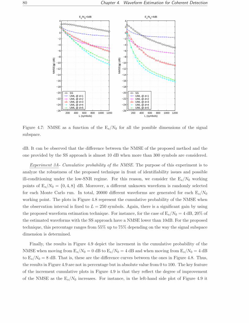
80 Chapter 4. Waveform Estimation for Coherent Detection
200 400 600 800 1000 1200−26
−24
−22
−20
−18
−16
−14
−12
−10
−8
−6
−4
−2
0
2
4
L (symbols)
NM
SE
(g)
(dB
)
Es/N
0=0dB
SSUML @ d=1UML @ d=2UML @ d=3UML @ d=4UML @ d=5
200 400 600 800 1000 1200−26
−24
−22
−20
−18
−16
−14
−12
−10
−8
−6
−4
−2
0
2
4
L (symbols)N
MS
E(g
) (d
B)
Es/N
0=4dB
SSUML @ d=1UML @ d=2UML @ d=3UML @ d=4UML @ d=5
Figure 4.7: NMSE as a function of the Es/N0 for all the possible dimensions of the signal
subspace.
dB. It can be observed that the difference between the NMSE of the proposed method and the
one provided by the SS approach is almost 10 dB when more than 300 symbols are considered.
Experiment 3A- Cumulative probability of the NMSE. The purpose of this experiment is to
analyze the robustness of the proposed technique in front of identifiability issues and possible
ill-conditioning under the low-SNR regime. For this reason, we consider the Es/N0 working
points of Es/N0 = {0, 4, 8} dB. Moreover, a different unknown waveform is randomly selected
for each Monte Carlo run. In total, 20000 different waveforms are generated for each Es/N0
working point. The plots in Figure 4.8 represent the cumulative probability of the NMSE when
the observation interval is fixed to L = 250 symbols. Again, there is a significant gain by using
the proposed waveform estimation technique. For instance, for the case of Es/N0 = 4 dB, 20% of
the estimated waveforms with the SS approach have a NMSE lower than 10dB. For the proposed
technique, this percentage ranges from 55% up to 75% depending on the way the signal subspace
dimension is determined.
Finally, the results in Figure 4.9 depict the increment in the cumulative probability of the
NMSE when moving from Es/N0 = 0 dB to Es/N0 = 4 dB and when moving from Es/N0 = 4 dB
to Es/N0 = 8 dB. That is, these are the difference curves between the ones in Figure 4.8. Thus,
the results in Figure 4.9 are not in percentage but in absolute value from 0 to 100. The key feature
of the increment cumulative plots in Figure 4.9 is that they reflect the degree of improvement
of the NMSE as the Es/N0 increases. For instance, in the left-hand side plot of Figure 4.9 it

4.5. Simulation Results 81
−24−20−16−12 −8 −4 0 40
10
20
30
40
50
60
70
80
90
100
NMSE (dB)
Cum
ulat
ive
prob
abili
ty (
% )
Es/N
0 = 0 dB
−24−20−16−12 −8 −4 0 40
10
20
30
40
50
60
70
80
90
100
NMSE (dB)
Cum
ulat
ive
prob
abili
ty (
% )
Es/N
0 = 4 dB
−24−20−16−12 −8 −4 0 40
10
20
30
40
50
60
70
80
90
100
NMSE (dB)
Cum
ulat
ive
prob
abili
ty (
% )
Es/N
0 = 8 dB
SSUML @ d
maxUML @ d
MAPUML @ d
opt
SSUML @ d
maxUML @ d
MAPUML @ d
opt
SSUML @ d
maxUML @ d
MAPUML @ d
opt
Figure 4.8: Cumulative distribution function (CDF) of the NMSE for Es/N0 = {0, 4, 8} dB.
is shown that the greatest improvement in NMSE is achieved by the population of waveform
estimates with NMSE=-10 dB. In contrast, and for the SS approach, the greatest improvement
in terms of NMSE is achieved by the population of waveform estimates with NMSE=-5 dB. This
corresponds to the position of the peaks for the Gaussian-like curves appearing in Figure 4.9.
4.5.2 Simulation results for UWB signals with binary APPM modulation
The proposed waveform estimation technique is of special interest for application to coherent
receivers with UWB signals, since they require robust channel state information for reliable
symbol detection. The closed-form solution and the estimation of the whole received waveform
(instead of just the propagation path delays and amplitudes) are the main features of the pro-
posed technique with respect to previous contributions in channel estimation for UWB signals.
Some valuable contributions can be found in [Lot00], [Car03], [Xu03b] or [Wil03], among
many other. However, most of these contributions do assume that the shape of the received
pulse is known (e.g. [Lot00], [Xu03b], [Wil03]) and thus, channel estimation is restricted to
the estimation of the time delays and amplitudes of the multipath rays through an iterative
optimization (e.g. [Lot00], [Car03]). As already mentioned in Section 4.1, the assumption of
known received pulse and a tapped-delay line model is not reasonable in practical UWB systems.
Many studies on the propagation of UWB signals conclude that the severe frequency-selective
and dispersive channel makes not possible for the receiver to know the shape of the received pulse

82 Chapter 4. Waveform Estimation for Coherent Detection
−24 −20 −16 −12 −8 −4 0 40
10
20
30
40
50
60
70
80
90
100
NMSE (dB)
∆ C
umul
ativ
e pr
obab
ility
−24 −20 −16 −12 −8 −4 0 40
10
20
30
40
50
60
70
80
90
100
NMSE (dB)
∆ C
umul
ativ
e pr
obab
ility
SSUML @ d
maxUML @ d
MAPUML @ d
opt
SSUML @ d
maxUML @ d
MAPUML @ d
opt
( Es/N
0=0dB → E
s/N
0=4dB ) ( E
s/N
0=4dB → E
s/N
0=8dB )
Figure 4.9: Incremental cumulative distribution of the NMSE from Es/N0 = 0 dB to Es/N0 = 4
dB (left) and from Es/N0 = 4 dB to Es/N0 = 8 dB (right).
in advance [Qiu02]. In addition to this, most approaches to channel estimation for UWB signals
do not assume the received signal to incur in interframe interference. For many techniques,
overlapping is not desired at the receiver, and thus, they space consecutive transmitted pulses
such that the maximum delay spread of the channel does not incur in overlapping (e.g. [Lot00],
[Car03]). In contrast, our closed-form approach to the waveform estimation problem allows the
received waveforms to be overlapped with each other within the symbol interval, which in turn,
determines the dimension of the signal subspace constraint.
In the simulation results to be presented herein, the simulation set-up comprises the trans-
mission of ultra-short pulses corresponding to the second derivative of the Gaussian pulse with
a total duration of 4 ns and modulated with binary APPM. The UWB channel is randomly
generated according to the channel model CM1 proposed by Intel [Foe03] whose power pro-
file is truncated to make the maximum delay spread of the multipath channel equal to 72 ns.
The pulse-position modulation involves a time-shift of 8 ns and the frame duration is set to 94
ns. The transmission of a single information bearing symbol is carried out by the repetition of
Nf = 64 frame intervals, and finally, the sampling period to Ts = 2 ns and the MAP model
order rule is adopted for determining the signal subspace dimension.
Experiment 1B- Mean estimated waveform for different noise realizations. For a randomly
selected received waveform, the results in Figure 4.10 depict the estimated waveform for 10
different noise realizations. For the sampling period and the channel model under consideration,

4.5. Simulation Results 83
the maximum finite time support of the unknown received waveform is Ng = 49 samples. As
shown in Figure 4.10, the estimates for the unknown waveform are pretty good for those initial
samples with significant SNR. However, the last samples of the selected unknown waveform are
close to zero, and thus, these samples are more difficult to estimate. A larger estimation variance
is exhibited in this null-region since there is no signal but only noise.
0 5 10 15 20 25 30 35 40 45 50−0.5
0
0.5
Samples
No
rma
lize
d a
mp
litu
de
0 5 10 15 20 25 30 35 40 45 50−0.5
0
0.5
Samples
No
rma
lize
d a
mp
litu
de
Mean estimated waveformTrue waveform
Estimated waveformTrue waveform
Figure 4.10: Example of waveform estimates for nonorthogonal binary-APPM transmission and
10 different noise realizations. The channel realization is fixed and generated from the channel
model CM1 proposed by Intel [Foe03].
Experiment 2B- Cumulative probability of the NMSE. For the case of Ng = 49 samples as
in Experiment 1B, the results in Figure 4.11 show the cumulative probability of the NMSE for
a total of 10000 randomly selected waveforms from the channel model in [Foe03]. Note that
the energy-per-frame to noise spectral density parameter Ef/N0 is adopted, since the waveform
estimation is performed on a frame-level basis (i.e. Nr = Nsf , with Nsf the number of samples
per frame). Because of the frame repetition structure of UWB signals, Ef/N0 = 1Nf
Es/N0,
so that the Ef/N0 coincides with the Es/N0 when there is no repetition and Nf = 1. The
evaluation of the NMSE is performed for different Ef/N0 values from 0 to 5 dB. Again, the
robustness of the proposed waveform estimation technique can be observed by noting that for
Ef/N0 = 5 dB, 90 % of the received waveform estimates have a NMSE ≤ -20 dB.

84 Chapter 4. Waveform Estimation for Coherent Detection
−30 −25 −20 −15 −10 −5 0 50
10
20
30
40
50
60
70
80
90
100
NMSE (dB)
Cum
ulat
ive
prob
abili
ty (
%)
Ef/N
0=5 dB
Ef/N
0=4 dB
Ef/N
0=3 dB
Ef/N
0=2 dB
Ef/N
0=1 dB
Ef/N
0=0 dB
Figure 4.11: Cumulative distribution function (CDF) of the NMSE for different Ef/N0 values.
4.6 Conclusions
A closed-form waveform estimation technique has been proposed based on the low-SNR UML cri-
terion. By introducing a signal subspace constraint and the vec operator, a subspace-compressed
low-SNR likelihood function is obtained which converts the nonlinear optimization problem
into a linear least-squares problem on the second-order statistics of the received signal. The
subspace-compressed approach can be understood as a principal component analysis, and thus,
a significant reduction in the computational burden is obtained through a tradeoff between bias
and variance. Another advantage of the subspace constraint is that it restricts the solution space
and hence, it avoids many of the effects of ill-conditioning and local-maxima of traditional ML
channel and waveform estimators. Finally, and for the low-SNR scenarios, simulation results
show the superior performance of the proposed technique with respect to existing closed-form
methods that are based on second-order statistics.
4.A Derivation of the low-SNR log-likelihood UML cost function 85
Appendix 4.A Derivation of the low-SNR log-likelihood UML
cost function
Under the low-SNR assumption, the likelihood function in (4.12) can be approximated by its
Taylor series expansion
Λ (r|g;x) ≈ C1
[1 +
2
σ2w
χ (r;g;x) +2
σ4w
χ2 (r;g;x)
](4.39)
with χ (r;g;x).=
∑P−1p=0 Re
[xH
p AHp r
]− 1
2
∑P−1p=0
∑P−1q=0 xH
q AHq Apxp. Next, since the transmitted
symbols are assumed to be all random, the symbol-independent likelihood function Λ (r|g) is
obtained as Λ (r|g) = Ex [Λ (r|g;x)]. Thus, the expectations Ex [χ (r;g;x)] and Ex
[χ2 (r;g;x)
]
are required. The first order moment of χ (r;g;x) is rather simple to calculate,
Ex [χ (r;g;x)] =P−1∑
p=0
Re[Ex
[xH
p
]AH
p r]− 1
2
P−1∑
p=0
P−1∑
q=0
Tr(AH
q ApEx
[xpx
Hq
])(4.40)
= − 1
2PTr (M) (4.41)
where, for the sake of simplicity, the new matrix M is defined as
M.=
P−1∑
p=0
ApAHp =
P−1∑
p=0
L−1∑
n=0
Kn,pggHKHn,p. (4.42)
In the derivation of the first order moment of χ (r;g;x) in (4.41) it has been taken into consider-
ation that Ex [xp] = 0 and Ex
[xpx
Hq
]= 1
P ILδpq. As for the second order moment of χ (r;g;x),
this requires further manipulation. As it is shown in Appendix 4.B, the second order moment
of χ (r;g;x) is found to be given by
Ex
[χ2 (r;g;x)
]=
1
2PrHMr +
1
4P‖M‖2
F +ζ
4, (4.43)
with ζ a constant term. Then, the low-SNR UML likelihood function results in
Λ (r|g) ≈ C1
[1 +
1
σ4wP
[−σ2
wTr (M) + rHMr +1
2‖M‖2
F +ζ
2P
]](4.44)
= C1
[1 +
1
σ4wP
[Tr
(M
[rrH − σ2
wIN
])+
1
2‖M‖2
F +ζ
2P
]]. (4.45)
Alternatively, the log-likelihood function L (r|g).= lnΛ (r|g) can be adopted. This is just a
formal consideration but it will allow us to relate the likelihood function in (4.45) with the
information criteria for determining the dimension of the signal subspace of the received data.
Thus, by taking into consideration that ln (1 + x) ≈ x when x → 0, the low-SNR UML log-
likelihood function can be expressed as
L (r|g) ≈ C2 +1
σ4wP
[Tr
(M
[rrH − σ2
wIN
])+
1
2‖M‖2
F +ζ
2P
], (4.46)
86 Chapter 4. Waveform Estimation for Coherent Detection
where C2 = lnC1. For an asymptotically large observation interval, let us decompose the (N×1)
vector of received samples r into a set of small (Nr × 1) and Nss-samples shifted vectors rn,
with rn.= [r(nNss), r(nNss + 1), . . . , r(nNss + Nr − 1)]T and Nr = max {Ng, Nss}. Note that
by setting the reduced observation interval to Nr = max {Ng, Nss}, a significant computational
complexity is saved while preserving the information regarding the unknown waveform. This
is because with Nr = max {Ng, Nss}, we guarantee that, at least, one of the waveform replicas
within the observation interval is not truncated. Finally, removing all the irrelevant constant
terms in (4.46) results in an equivalent low-SNR UML log-likelihood function, namely L′ (r|g),
which is defined as follows,
L′ (r|g) = Tr(M
[R − σ2
wINr
])+
1
2‖M‖2
F . (4.47)
with M the (Nr × Nr) truncated version of matrix M in (4.42). That is,
M.=
Lp−1∑
p=0
Kr∑
n=−Kr
Kn,pggHKHn,p (4.48)
with Kr the one-sided number of Nss-samples shifted replicas of g, and Lp the number of N∆-
samples shifted replicas of g, both within an observation interval of Nr samples. In addition, Kn,p
is the (Nr × Ng) truncated version of matrix Kn,p. In Matlab notation, Kn,p.= Kn,p (1 : Nr, :).
Note that in (4.47), the initial observation interval of N samples has been asymptotically (L →∞) folded into a smaller observation interval of Nr samples. Consequently, the (N ×N) sample
covariance matrix rrH in (4.46) is converted into the (Nr × Nr) synchronous autocorrelation
matrix R. Thus, the second-order statistics of the received signal become the sufficient statistics
for the problem under consideration.
Appendix 4.B Derivation of the Second Order Moment of
χ (r;g;x)
From the definition of χ (r;g;x) in (4.13) it can be found that,
χ2 (r;g;x) =
P−1∑
p=0
Re[xH
p AHp r
]
2
︸ ︷︷ ︸B1
−
P−1∑
p=0
Re[xH
p AHp r
]
P−1∑
p=0
P−1∑
q=0
xHq AH
q Apxp
︸ ︷︷ ︸B2
(4.49)
+1
4
P−1∑
p=0
P−1∑
q=0
xHq AH
q Apxp
2
︸ ︷︷ ︸B3
. (4.50)
Therefore, the evaluation of Ex
[χ2 (r;g;x)
]involves the expectation of B1, B2 and B3 in (4.50).
4.B Derivation of the Second Order Moment of χ (r;g;x) 87
B1: This quadratic term can be first expanded, and then, by taking into consideration that
Ex
[xpx
Hq
]= 1
P ILδpq it is found that,
Ex
P−1∑
p=0
Re[xH
p AHp r
]
2 =
1
2PrHMr (4.51)
with M defined in (4.42).
B2: This term vanishes because it depends on the odd moments of the transmitted symbols.
B3: This term should be first expanded as,
P−1∑
p=0
P−1∑
q=0
xHq AH
q Apxp
2
=P−1∑
p=0
P−1∑
q=0
P−1∑
m=0
P−1∑
n=0
Tr(AH
p AqxqxHmAH
mAnxnxHp
)(4.52)
= vecT(x∗
mxTq AT
q A∗p
)vec
(AH
mAnxnxHp
), (4.53)
where it has been used the property Tr (BC) = vecT(BT
)vec (C) for any (n× q) matrix
B and any (q × p) matrix C. In addition, and for any (m × n) matrix A, it is found that
vec (ABC) =(CT ⊗ A
)vec (B) with ⊗ the Kronecker product [Har00, p.342]. Therefore,
P−1∑
p=0
P−1∑
q=0
xHq AH
q Apxp
2
= vecT(x∗
mxTq
) [(AT
q A∗p
)⊗ IL
] [IL ⊗
(AH
mAn
)]vec
(xnx
Hp
)
= vecH(xmxH
q
) [(AT
q A∗p
)⊗
(AH
mAn
)]vec
(xnx
Hp
)(4.54)
= Tr([(
ATq A∗
p
)⊗
(AH
mAn
)]vec
(xnx
Hp
)vecH
(xmxH
q
)).(4.55)
At this point, the expectation with respect to the transmitted symbols can be intro-
duced in (4.55). Then, the main focus of interest is the computation of the term
Ex
[vec
(xnx
Hp
)vecH
(xmxH
q
)]. The result for the particular case in which n = p = m = q
can be found in [Vil05], and with this help, the general expression can be found after te-
dious algebraic manipulations. As a result, the expectation with respect to the transmitted
symbols of (4.55) can be summarized as follows,
Ex
P−1∑
p=0
P−1∑
q=0
xHq AH
q Apxp
2 =
1
P‖M‖2
F + ζ (4.56)
with ζ a term that is asymptotically constant for large data records, and it just depends
on the energy of the received waveform. In the derivation of (4.56) it has been taken into
consideration that for P > 1 (i.e. with PPM and APPM modulations) there is enough
separation between consecutive pulses so as to avoid intersymbol interference, that is,
Ng ≤ Nss. Then, the product of matrices in the form AHq Ap results in a diagonal matrix
for any value of {p, q}.

88 Chapter 4. Waveform Estimation for Coherent Detection
From the above considerations, we finally have that
Ex
[χ2 (r;g;x)
]=
1
2PrHMr +
1
4P‖M‖2
F +ζ
4. (4.57)
Appendix 4.C Application of the vec operator to the low-SNR
UML log-likelihood cost function
By using the vec operator, the low-SNR UML cost function in (4.47) can be recast as,
L′ (r|g) = vecT(M∗
)vec
(R − σ2
wINr
)+
1
2vecT
(M∗
)vec
(M
)(4.58)
with (·)∗ the complex conjugate. Let us further manipulate the terms involving vec(M
)by
taking into consideration the subspace-constraint in (4.19) and the relationship vec (ABC) =(CT ⊗ A
)vec (B),
vec(M
)= vec
Kr∑
n=−Kr
Lp−1∑
p=0
Kn,pggHKHn,p
=
Kr∑
n=−Kr
Lp−1∑
p=0
vec(Kn,pUsαα
HUHs KH
n,p
)
=
Kr∑
n=−Kr
Lp−1∑
p=0
(Kn,pU
∗s
)⊗
(Kn,pUs
) vec
(αα
H). (4.59)
Next, let us define the (N2r × 1) vector rv, the (N2
r × d2) matrix Q and the (d2 × 1) vector αv
as,
rv.= vec
(R − σ2
wINr
), (4.60)
Q.=
Kr∑
n=−Kr
Lp−1∑
p=0
(Kn,pU
∗s
)⊗
(Kn,pUs
), (4.61)
αv.= vec
(αα
H). (4.62)
Then, the low-SNR UML cost function in (4.58) results in
L′ (r|g) = αHv QH rv +
1
2α
Hv QHQαv. (4.63)

Chapter 5
Non-Coherent Detection of Random
UWB Signals
5.1 Introduction
One of the main problems with the transmission of UWB signals is that the received waveform
has very little resemblance with the original transmitted pulse. As already mentioned in Section
2.4, some of the reasons for this behavior are the following. First, the solid state pulse generating
devices exhibit implementation imperfections such as random timing jitter or asymmetric polar-
ity rising times that prevent the transmitted pulses to be all exactly the same [Win02]. Second,
the radiating elements are found to differentiate the transmitted pulse [Zio92], [Mir01] and a
different distortion is experienced depending on the angle of radiation [Kon05], [Wan05]. Third,
the propagation physics of UWB signals make the channel response to be terribly frequency-
dependent and this causes a severe pulse distortion at the receiver [Qiu02], [Qiu05]. Fourth,
experimental results show that the pulse distortion is also path-dependent and thus, different
pulse distortions are experienced when propagating through different paths and through differ-
ent materials [Cra02]. As a result of all these degradations, the end-to-end channel response can
reasonably be assumed to be time-varying. This is particularly true when the propagation paths
change as a result of the relative movement between transmitter and receiver. In addition, the
paths can also change as a result of moving scatterers like moving persons in indoor scenarios
[Sch05b] and thus it is reasonable to assume the received waveform as random.
Because of the above considerations, the adoption of coherent receivers (i.e the assumption
of channel state information) is restricted to those applications where slow channel variations
are experienced and significant computational complexity is available at the receiver. This is
due to the fact that the large multipath resolution of UWB signals makes the computation of
fast and accurate channel estimates a challenging and computationally demanding task. When
89

90 Chapter 5. Non-Coherent Detection
such a computational burden is not available, there is no choice but to resort to non-coherent
receivers [Car06a].
At this point, note that many of the traditional signal processing techniques for narrowband
communication systems cannot be adopted anymore. In particular, the popular receiver based
on a filter matched to the transmitted pulse can no longer be considered since the received
pulse has no resemblance with the transmitted one. However, many contributions on UWB
communication systems ignore this problem and they still formulate the optimal receiver by
applying the well-known matched filter principle to all the propagation paths (see, for instance,
[Gez04], [Chu04], [Oh05] or [Tan05a] among many other).
Symbol detection for UWB signals when no channel state information is available is also
considered in [D’A05], [Car06a] or [Fen03], among many other. Nevertheless, an unknown de-
terministic approach is considered where the received waveform is assumed to be unknown but
constant during all the observation interval. Other approaches consider the problem of waveform
time-variation by adopting transmitted reference (TR) signaling, which is based on the transmis-
sion of a reference pulse prior to each data modulated pulse [Rus64], [Hoc02], [Fra03], [Cha05].
In that way, noisy channel state information is provided by the received unmodulated pulses
themselves. However, this comes at the expense of an efficiency loss due to the transmission of
unmodulated pulses and at the end, a coherent receiver is required once again.
Contrary to the deterministic approach, herein the emphasis is placed on treating the re-
ceived signal as random. Since no channel state information is assumed at the receiver, coherent
detection cannot be applied and non-coherent techniques must be adopted based on the under-
lying statistics of the received data. Clearly, this is a problem of random signal detection, a topic
that has received significant attention in the last decades with many important contributions in
RADAR and SONAR applications [Van03], [Kay98], among many other.
In this sense, the goal of this chapter is to address the optimal non-coherent symbol detection
problem of PPM modulated UWB signals when the received waveforms are assumed to be all
random. For the sake of clarity, binary-PPM is considered but the extension to higher order
constellations can be done in a straightforward manner. In particular, the symbol detection
problem is formulated here within the framework of likelihood ratio testing for the low-SNR
regime. The low-SNR assumption is an important part of this study since it can be considered
as a realistic hypothesis to the real operating conditions of UWB systems. Once the optimal
symbol decision statistics are derived, different practical cases of interest are further analyzed.
For instance, an information theoretic based receiver is proposed as a tradeoff between perfor-
mance and implementation complexity in the presence of correlated scattering. The result is a
gradient based scheme which provides the best and simplest receiver filter for maximizing the
divergence measure of the symbol decision problem. Simulation results are provided to evalu-
ate the performance of the proposed receivers and insightful links are established with existing

5.2. Signal Model and Problem Statement 91
contributions in the recent literature.
The chapter is organized as follows. The signal model and the problem statement are in-
troduced in Section 5.2. The determination of the actual propagation conditions is presented
in Section 5.3 by estimating the covariance matrix of the unknown random channel. Next, the
optimal non-coherent symbol decision rule is derived in Section 5.4 for the low-SNR regime.
The particularization of this symbol decision strategy to the case of uncorrelated and correlated
scattering is analyzed in Section 5.5 and Section 5.6, respectively. Finally, simulation results are
discussed in Section 5.7 and conclusions are drawn in Section 5.8.
5.2 Signal Model and Problem Statement
5.2.1 Modulation format
The signal model to be considered in this chapter assumes the transmission of ultra-short pulses
with binary pulse-position modulation (2-PPM). It is important to recall that PAM cannot be
considered since it does not allow non-coherent detection.
As it is standard in most UWB communication systems, the transmission of every single
information bearing symbol is implemented by the repetition of Nf low-power pulses. Each
of these pulses is confined within a frame duration of Nsf samples that must be long enough
so as to avoid interframe interference between consecutive frames. Consequently, the frame
duration must encompass the maximum delay spread of the channel and the maximum time-
shift introduced by the PPM modulation and the time-hopping (TH) sequence. In this chapter,
however, no TH sequence is assumed. The reason is that, since we focus on the symbol decision
problem, the TH sequence is assumed to have been previously acquired in a prior stage of the
receiver.
At the receiver, the transmitted pulses arrive in the form of distorted waveforms. The
degradation is caused by the inherent distortion produced by the wideband radiating elements,
but especially, because of the propagation physics of UWB signals. In this sense, and similarly to
[Car06b], an unstructured approach is adopted for modeling the propagation of the transmitted
signal. That is, we completely disregard the paths of the propagation channel and we just
consider the received waveform as a whole. This received waveform is denoted by the discrete-
time notation g(k), and the received signal can be expressed as,
r(k) =∞∑
n=−∞
cn
Nf−1∑
i=0
gn,i (k − dnN∆ − iNsf − nNss) + n(k) (5.1)
with N∆ the number of samples for the PPM time-shift, Nsf the number of samples per frame
(i.e. the frame duration) and Nss the number of samples per symbol (i.e. the symbol duration).

92 Chapter 5. Non-Coherent Detection
Because of the frame repetition within the symbol duration, the number of samples per symbol is
Nss.= NfNsf . Since binary PPM is adopted, pulse-position symbols are restricted to dn = {0, 1}.
Moreover, the sequence cn = {−1, 1} accounts for the polarity randomization code that is
introduced in order to avoid the existence of spectral lines that may violate spectral regulations
[Nak03]. Finally, n(k) includes the contribution of both the thermal noise and the interference
signal. That is, n(k) = w(k) + i(k) with w(k) the zero-mean Gaussian samples of the thermal
noise with variance σ2w and i(k) the interference signal to be described in Section 5.2.2.
Regarding the received waveform, note that gn,i(k) in (5.1) stands for the received waveform
corresponding to the n-th symbol and the i-th frame. The received waveforms gn,i(k) have a
maximum finite time support of Ng samples and the indexation {n, i} is consistent with the fact
that the received waveform may differ from frame to frame. For instance, this variation of the
received waveforms may be caused by the relative movement between transmitter and receiver
but also because of moving scatterers like moving persons [Sch05b]. Moreover, the signal model
in (5.1) assumes that the coarse frame-timing error has been previously acquired, a topic to be
discussed in Chapter 6. As a result, the starting time of the symbol period is known up to a
fraction of the frame duration and this frame-level residual timing error is incorporated in the
shape of the unknown waveform.
At this point, let us express the signal model in (5.1) into a more compact matrix notation.
To this end, let us divide the observation interval into a total of L segments rn, each with a length
equal to the symbol duration Nss. Thus, the observation interval assumes the transmission of
L binary-PPM symbols. Similarly, let us divide each received symbol vector rn into a total
of Nf segments rn,i corresponding to the Nf frames within a symbol duration. That is, rn =[rTn,0, r
Tn,1, . . . , r
Tn,Nf−1
]Twith rn,i a (Nsf × 1) vector with the samples of the i-the frame of the
n-th symbol. According to the structure of binary pulse position modulation, the received signal
for each frame interval can be expressed as follows,
rn,i =
cnΠgn,i + nn,i : dn = 0
cnJN∆Πgn,i + nn,i : dn = 1 .
(5.2)
Matrices Π and JN∆in (5.2) are a (Nsf × Ng) zero-padding matrix and a (Nsf × Nsf ) N∆-
samples time-shift matrix, respectively. Finally, the (Ng × 1) vector gn,i incorporates the Ng
samples of the received waveform for the n-th symbol and i-th frame, and nn,i the corresponding
samples of the noise and interference contribution.
5.2.2 Interference signal model
The two major characteristics of UWB communication systems are their very large spectral
occupancy and their very low power spectral density. The spectral occupancy of UWB signals
5.2. Signal Model and Problem Statement 93
is on the order of a few GHz and this forces UWB signals to coexist with most of the existing
wireless communication systems. However, the very large spectral occupancy of UWB signals
makes current wireless communication systems to be perceived as narrowband interferences
by a UWB receiver. Since spectral regulations restrict the radiation of UWB signals within
the band from 3 GHz to 10 GHz, it turns out that the most significant source of interference
are IEEE 802.11a WLAN devices, whose central frequency is located around 5 GHz and the
transmitted bandwidth is about 20 MHz. Moreover, these WLAN interference sources can also
be considered to be high-power sources compared to UWB signals [Sah05]. For instance, the
maximum transmitted power for IEEE 802.11a devices is about 17dBm/Mhz. For the case of
UWB signals, the maximum allowed transmitted power is -41.3dB/MHz according to the FCC
spectral regulations. Therefore, an IEEE 802.11a system with 20 MHz of bandwidth results
in a total transmitted power of PIEEE802.11amax = 30 dBm. In contrast, an UWB system with a
maximum bandwidth of 7 GHz results in a total transmitted power of PUWBmax = −2.85 dBm.
That is, the transmitted power of an IEEE 802.11a device is more than 30 dB higher than that
of an UWB system.
In order to model the interfering signals arriving to an UWB receiver, the Gaussian signal
model is assumed herein. Similarly to [Chu04] or [Ber02], the interference signals are assumed to
be discrete-time zero-mean passband Gaussian random processes whose spectral density SI(f)
is characterized by the central frequency fI and the bandwidth occupancy BWI as follows,
SI(f) =
{NI2 , fI − BWI
2 ≤ |f | ≤ fI + BWI2
0, otherwise.(5.3)
Consequently the interference i(k) for n(k) = w(k)+i(k) in (5.1) is characterized by a covariance
matrix CI whose (i, j) entries are given by
[CI]i,j = PIsinc (BWI (i − j)) cos (2πfI (i − j)) (5.4)
with PI = NI · BWI the interference power.
5.2.3 UWB channel model and operating conditions
The optimal design of a communication system must take into consideration the propagation
conditions of the transmitted signal in the way to the receiver. However many issues related
with the propagation conditions of UWB signals are still under study. The main reason is
that, although UWB technology has been around since the 60s, most channel measurement
campaigns are being performed in the recent years. Thus, there is still a lot to be learned
about the propagation characteristics of UWB signals and more measurement campaigns are
still required [Mol05].

94 Chapter 5. Non-Coherent Detection
The most common characteristic of UWB transmissions is the extremely frequency-, path-
, and angle-dependent transfer function. From a stochastic point of the view, some authors
indicate that the statistical modeling of the measured small-scale fading is related to the Nak-
agami distribution (e.g. [Cas02a]), or to the lognormal distribution (e.g. [Foe03]). These results
are indeed included in the IEEE 802.15.3a channel models which are especially devoted to high
data-rate UWB systems operating in residential and office environments [Foe03]. However, UWB
channels measured by other authors are found to be not so different from traditional channels.
Measurement campaigns were carried out with both moving and fixed terminals in open space
environments such as a lobby (e.g. [Sch05b], [Sch05c]) and in industrial environments (e.g.
[Kar04]). For these propagation environments, the small-scale fading statistics of the received
waveforms were found to be closer to the traditional Rayleigh and Rice distributions rather than
to the Nakagami and lognormal distributions assumed in the IEEE 802.15.3a channel models.
Similarly to traditional wideband channels, the Rayleigh distribution was found to apply with
moving terminals whereas the Rice distribution was found to apply with static terminals. This
is somehow surprising because the very large bandwidth of UWB signals is often argued for
not assuming the traditional Gaussian assumption for the tap amplitudes. These new results
were included in the IEEE 802.15.4a channel models [Mol04] which were intended to cover the
gap left by the IEEE 802.15.3a channel models and to focus on low data-rate applications that
usually operate in industrial, outdoor or rural environments. See Figure 5.1 and Figure 5.2 to
notice the difference between the statistical characterization of non-line-of-sight channels within
the IEEE 802.15.3a/4 standards.
In the sequel, the Gaussian approach suggested by [Sch05b], [Sch05c] or [Kar04] is adopted
for mathematical tractability. Consequently, the samples of the received waveforms are modeled
by a zero-mean random Gaussian process driven by a (Ng × Ng) covariance matrix Cg.
According to the signal model in Section 5.2, let us indicate the hypothesis of transmitting
dn = 1 by H+ and the hypothesis of transmitting dn = 0 by H−. Under the hypothesis H+, the
conditional probability density function for the n-th received symbol is given by the multivariate
Gaussian probability density function as follows,
f (rn|H+;Cg) =
Nf−1∏
i=0
1
(2π)Nsf /2 det1/2 (C+ + CN)exp
(−1
2rTn,i (C+ + CN)−1 rn,i
)(5.5)
with C+.= ΠCgΠ
T the covariance matrix for the signal received under H+ and CN.= σ2
wI +
CI the covariance matrix for the Gaussian contribution of both the thermal noise and the
narrowband interference. Similarly, the probability density function under the hypothesis H−
is found by substituting C+ with C−.= JN∆
ΠCgΠTJT
N∆in (5.5).

5.2. Signal Model and Problem Statement 95
−15 −10 −5 0 5 10 150
5000
10000Histogram for IEEE 802.15.3a CM3
rn,i
(10)
−15 −10 −5 0 5 10 150
2000
4000
6000
8000rn,i
(50)
−15 −10 −5 0 5 10 150
2000
4000
6000rn,i
(150)
Figure 5.1: Histogram of received waveforms at the sample bins k = {10, 50, 150} under the
channel model IEEE 802.15.3a CM3 (non-line-of-sight) .
−15 −10 −5 0 5 10 150
200
400
600
800Histogram for IEEE 802.15.4a CM8
rn,i
(10)
−15 −10 −5 0 5 10 150
200
400
600
800rn,i
(50)
−15 −10 −5 0 5 10 150
500
1000rn,i
(150)
Figure 5.2: Histogram of received waveforms at the sample bins k = {10, 50, 150} under the
channel model IEEE 802.15.4 CM8 (industrial non-line-of-sight) .

96 Chapter 5. Non-Coherent Detection
It is important to note that the probability density function in (5.5) is conditioned on the
covariance matrix Cg. This covariance matrix Cg is unknown since it conveys the information
regarding the second-order statistics of the actual received waveforms, which are usually un-
known and depend on the particular transmission/reception set-up and propagation conditions.
Therefore the covariance matrix Cg can be regarded as a nuisance parameter that has to be
estimated. Replacing Cg with a suitable estimate leads to a compressed or conditional approach
where the symbol decision statistics do not depend on Cg anymore. This conditional approach
is presented in Section 5.5 and Section 5.6 whereas the estimate for Cg is to be presented next
in Section 5.3.
5.2.4 Receiver architecture
The system architecture to be considered in this chapter is represented in the block diagram
of Figure 5.3. It represents a fully digital non-coherent receiver where the incoming signal is
synchronized at the frame-level in a non-coherent fashion. The purpose to include the frame-
synchronization as the first step of this receiver is due to the fact that, for the subsequent
analysis within this chapter, the signal to be considered for the symbol detection is assumed to
be frame-synchronized. Frame-synchronization is possible to be performed prior to the chan-
nel characterization since the proposed non-coherent frame synchronization method is able to
succeed in the absence of any channel knowledge. This will be discussed in more detailed in
Chapter 6.
Figure 5.3: Block diagram of the receiver architecture to be considered in this chapter.
5.3 Estimation of the Unknown Channel Covariance Matrix
As a result of the unknown distortion suffered by the transmitted pulse, the covariance matrix
Cg for the Gaussian random received waveform model is also unknown. However, this covariance
matrix is ultimately required for the evaluation of the symbol decision statistics and it must be
estimated from the received data. To this end, an estimate for Cg is presented herein which is
based on the least-squares principle. The key point is to exploit the structure of the frame-level
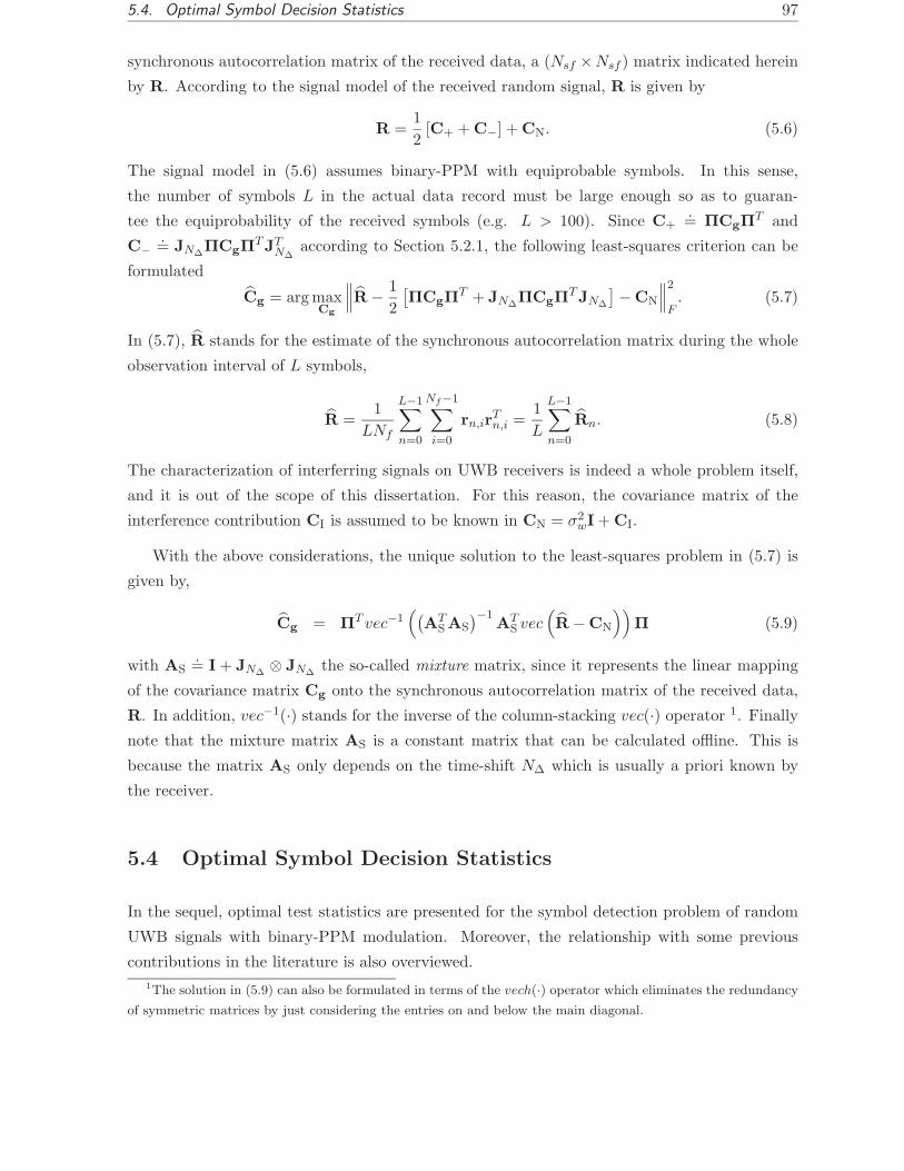
5.4. Optimal Symbol Decision Statistics 97
synchronous autocorrelation matrix of the received data, a (Nsf ×Nsf ) matrix indicated herein
by R. According to the signal model of the received random signal, R is given by
R =1
2[C+ + C−] + CN. (5.6)
The signal model in (5.6) assumes binary-PPM with equiprobable symbols. In this sense,
the number of symbols L in the actual data record must be large enough so as to guaran-
tee the equiprobability of the received symbols (e.g. L > 100). Since C+.= ΠCgΠ
T and
C−.= JN∆
ΠCgΠTJT
N∆according to Section 5.2.1, the following least-squares criterion can be
formulated
Cg = arg maxCg
∥∥∥R − 1
2
[ΠCgΠ
T + JN∆ΠCgΠ
TJN∆
]− CN
∥∥∥2
F. (5.7)
In (5.7), R stands for the estimate of the synchronous autocorrelation matrix during the whole
observation interval of L symbols,
R =1
LNf
L−1∑
n=0
Nf−1∑
i=0
rn,irTn,i =
1
L
L−1∑
n=0
Rn. (5.8)
The characterization of interferring signals on UWB receivers is indeed a whole problem itself,
and it is out of the scope of this dissertation. For this reason, the covariance matrix of the
interference contribution CI is assumed to be known in CN = σ2wI + CI.
With the above considerations, the unique solution to the least-squares problem in (5.7) is
given by,
Cg = ΠT vec−1((
ATS AS
)−1AT
S vec(R − CN
))Π (5.9)
with AS.= I + JN∆
⊗ JN∆the so-called mixture matrix, since it represents the linear mapping
of the covariance matrix Cg onto the synchronous autocorrelation matrix of the received data,
R. In addition, vec−1(·) stands for the inverse of the column-stacking vec(·) operator 1. Finally
note that the mixture matrix AS is a constant matrix that can be calculated offline. This is
because the matrix AS only depends on the time-shift N∆ which is usually a priori known by
the receiver.
5.4 Optimal Symbol Decision Statistics
In the sequel, optimal test statistics are presented for the symbol detection problem of random
UWB signals with binary-PPM modulation. Moreover, the relationship with some previous
contributions in the literature is also overviewed.
1The solution in (5.9) can also be formulated in terms of the vech(·) operator which eliminates the redundancy
of symmetric matrices by just considering the entries on and below the main diagonal.

98 Chapter 5. Non-Coherent Detection
5.4.1 Log-GLRT for the binary-PPM decision problem
Since the received waveforms are assumed to be all random, the symbol detection problem must
rely on the statistical properties of the received waveforms rather than on their particular shape.
The optimal symbol decision statistics will be derived based on the generalized likelihood ratio
test (GLRT) which maximizes the probability of detection for a given probability of false alarm
[Kay98]. The GLRT just requires the knowledge of the probability density function of the signal
hypothesis to be considered, and for the problem under consideration, two hypothesis must be
decided depending on whether dn = 1 or dn = 0. Thus, the GLRT is obtained by evaluating the
ratio
Λ(rn|Cg).=
f (rn|H+;Cg)
f (rn|H−;Cg)(5.10)
with f (rn|H+;Cg) defined in (5.5), and deciding dn = 1 when Λ(rn|Cg) > 1 or dn = 0 when
Λ(rn|Cg) < 1. Alternatively, the logarithm can be taken in both sides of (5.10) resulting in the
log-GLRT,
L (rn|Cg).= log Λ(rn|Cg) (5.11)
= logf (rn|H+;Cg)
f (rn|H−;Cg)(5.12)
from which a simple and compact decision metric can be obtained.
At this point, two important assumptions are considered. First, the low power of UWB
signals allows us to assume that both the noise and the interference signals can be considered
high power sources. Second, the very large bandwidth of UWB signals allows us to assume
that existing wireless transmission systems are narrowband interferences. This second assump-
tion is reasonable since the bandwidth of UWB signals is on the order of a few GHz whereas
the bandwidth of existing wideband wireless systems is on the order of 10 to 20 MHz (e.g.
IEEE802.11a/b/g wireless LAN devices).
With the above considerations, the optimal decision metric for random UWB signals with
binary-PPM modulation is given by the log-GLRT,
L′(rn|Cg) = Tr([
C+ − C−
]Rn
)(5.13)
where {C+,C−} are the frame-level covariance matrices for the signal model under the hypoth-
esis {H+,H−}, and Rn is the estimate of the frame-level synchronous autocorrelation matrix
during the n-th received symbol duration. That is,
Rn.=
1
Nf
Nf−1∑
i=0
rn,irTn,i. (5.14)
Moreover, L′ (rn|Cg) in (5.13) is obtained from L (rn|Cg) in (5.12) by omitting all the irrelevant
constant terms. All the analytic derivations to obtain (5.13) are omitted for clarity reasons but
they are all given in Appendix 5.A and Appendix 5.B.

5.4. Optimal Symbol Decision Statistics 99
Finally, and with the above considerations, the symbol decision rule can be implemented as
dn =1
2
[1 + sign
{L′(rn|Cg)
}]. (5.15)
An important point with respect to the result in (5.13) is that the log-GLRT in (5.13) depends
on the covariance matrix of the random end-to-end channel response Cg. This is due to the fact
that both C+ and C− are based on Cg according to Section 5.2.3. Since the covariance matrix
Cg is unknown, it must be first estimated from the incoming data in order to evaluate the
log-GLRT. At this point, the estimate for Cg already presented in (5.9) can be incorporated.
By doing so, the log-GLRT is compressed with the information regarding the actual channel
conditions, and this results in the contributions to be presented later on in Section 5.5 and
Section 5.6 for the case of uncorrelated and correlated scattering, respectively.
5.4.2 Relationship of the proposed log-GLRT with existing literature
The log-GLRT presented in (5.13) is a rather general result for the symbol detection problem of
binary-PPM UWB signals under the assumptions of low signal-to-noise ratio and low signal-to-
interference ratio. In this sense, it is interesting to note that many of the receivers heuristically
proposed in the existing literature are indeed particular cases of the more general result in (5.13).
First of all, the log-GLRT can be understood as a balanced second-order matched filter. Let
us denote the difference matrix C+ − C− in (5.13) by P, that is, P.= C+ − C−. Thus, matrix
P becomes a correlation template for deciding between the hypothesis H+ and H−, similarly
to what occurs for the binary symbol detection problem with deterministic signals. In fact, for
the case of deterministic signals, the coherent receiver is based on a correlation template with
impulse response p(k) = g(k) − g(k − N∆), being g(k) the transmitted pulse [Win00]. This is
indeed the coherent scalar version of the non-coherent second-order template P.
Another important point to be highlighted is that no matrices are required to be inverted
in the test statistics in (5.13). This is in contrast with traditional detectors for random signals,
where the inverse of the involved covariance matrices is usually required [Van03]. In fact, this
matrix inversion can be understood as a way of emphasizing the noise subspace since most of
the traditional detectors are based on exploiting the deterministic structure of this subspace.
Contrary to this approach, it is important to remark that the result obtained in (5.13) is indeed
exploiting the signal subspace by projecting the received data onto the space defined by the
signal covariance matrices. This is a consequence of the low SNR approach adopted herein and
it is expected to provide a more robust performance in front of the noise at the expense of a
limiting floor effect for the high SNR scenarios. This floor effect phenomenon is explained as
the degradation resulting from the noise introduced by the algorithm itself [Gar80] and it is
commonly exhibited by most low-SNR techniques.

100 Chapter 5. Non-Coherent Detection
As it will be shown later on, the result in (5.13) includes the energy-detector receiver
[Rab04a], [Wei04]. This is a suboptimal receiver that can be obtained from (5.13) by forc-
ing uncorrelated scattering with a constant power delay profile. The eigen-based receiver in
[Zha05b] can also be obtained from (5.13) by taking just the principal eigenvector of P, which is
found to be the best deterministic template for linear filtering the random received data. Finally,
the test statistic in (5.13) under the assumption of uncorrelated scattering will be shown to in-
clude the receiver proposed in [Wei05] where the power delay profile of the channel is assumed
to be known.
5.5 Optimal Receiver under the Uncorrelated Scattering As-
sumption
In the presence of uncorrelated scattering (US) the covariance matrix of the received waveforms
simplifies to a diagonal matrix. That is2,
Cg = diag (γ) (5.16)
with
γ = [γ(0), γ(1), . . . , γ(Ng − 1)]T (5.17)
the power-delay profile (PDP) of the end-to-end channel response (i.e. the PDP of the received
waveforms). Consequently the frame-level covariance matrices for the hypothesis {H+,H−}become
C+ = diag (γ) , (5.18)
C− = diag (JN∆γ) , (5.19)
respectively. Note that γ.= Πγ is the (Nsf ×1) zero-padded version of the (Ng ×1) power-delay
profile indicated by γ in (5.16).
It is first interesting to keep in mind the expression of the log-GLRT in (5.13) and assume
for a while that the power-delay profile is a priori known at the receiver. By doing so, Section
5.5.1 provides insightful relationships with existing contributions in the current literature. In
Section 5.5.2, however, the power-delay profile will be assumed to be unknown. In that case,
a conditional log-GLRT will be presented by compressing the unknown parameter with the
information available from the incoming data.
2diag(X), when X is a matrix, returns a vector formed from the elements of the main diagonal of X. Similarly,
diag(x), when x is a vector, returns a diagonal matrix formed from the elements of x.

5.5. Optimal Receiver under the Uncorrelated Scattering Assumption 101
5.5.1 Log-GLRT under the assumption of known power-delay profile
Initially, let us assume that the power-delay profile is a priori known at the receiver. Then, the
log-GLRT in (5.13) results in
L′(rn) = Tr(diag (γ − JN∆
γ) Rn
)= Tr
(diag(w)Rn
)(5.20)
=
Nsf−1∑
k=0
w(k)
Nf−1∑
i=0
r2n,i(k) (5.21)
where the optimal correlation template w is defined as w.= γ − JN∆
γ and rn,i(k) stands for
the k-th sample within vector rn,i. That is, rn,i(k).= [rn,i]k. The receiver implementation for
the test statistics in (5.21) is shown in Figure 5.4.
Figure 5.4: Optimal detector for random binary-PPM signals with uncorrelated scattering when
the PDP is a priori known.
Next, the following relationships with existing contributions can be established. Firstly, the
structure in (5.21) is similar to the MLRP receiver in [Wei05] where the received waveform was
modeled as a continuous-time random process given by the product of a white Gaussian noise
and a low-pass signal. However, the weighting function w(k) for the MLRP receiver is found to
depend on the inverse of the noise power and thus, it may be significantly more unstable. On
the contrary, the result in (5.21) shows that the weighting function w(k) does not depend on the
noise power but just on the power-delay profile and thus, a more robust and stable performance
is expected.
Secondly, the PDP-receiver proposed in (5.21) particularizes to the well-known energy-
detector receiver [Rab04a] when the power-delay profile is constant. In this case, γ = γ1Ng
for some positive constant γ and 1n an all ones (n × 1) vector3. Then the weighting function
w(k) becomes the difference of two noncoherent integrations of received samples.
5.5.2 Conditional log-GLRT
A possible approach when the power-delay profile γ is not a priori known is to consider that
it is an unknown deterministic nuisance parameter that has to be estimated. In this sense, an
3When omitted, the dimensions of the all ones vector 1 and the identity matrix I are (Nsf ×1) and (Nsf ×Nsf ),
respectively, with Nsf the number of samples per frame.

102 Chapter 5. Non-Coherent Detection
estimate for the zero-padded power-delay profile γ is proposed here based on the least-squares
criterion introduced in (5.7). For the case of uncorrelated scattering the cost function in (5.7)
simplifies to
γ = arg maxγ
∥∥∥diag(R) − 1
2(I + JN∆
) γ −(σ2
w + PI
)1∥∥∥
2. (5.22)
Therefore, the least-squares estimate for the zero-padded power-delay profile γ is given by
γ =(BT
S BS
)−1BT
S diag(R −
(σ2
w + PI
)I)
(5.23)
with BS.= I+JN∆
the mixture matrix representing the linear mapping of the power-delay profile
onto the synchronous autocorrelation of the received data. Next, (5.23) is substituted into the
log-GLRT in (5.13). As a result, and by taking into consideration the diagonal structure of Rn
under the US assumption, the test statistics are given by
L′(rn) =(γ − JN∆
γ)T
diag(Rn
)= γT
(I − JN∆)T diag
(Rn
)(5.24)
= diagT(R −
(σ2
w + PI
)I)BS
(BT
S BS
)−1BT
Ddiag(Rn
)(5.25)
with BD.= I − JN∆
the separation matrix representing the linear mapping of the power-delay
profile onto the weighting function w in (5.20). Since the mixture matrix BS is full rank then(BT
S BS
)−1= B−1
S
(BT
S
)−1and the log-GLRT in (5.25) can be recast as
L′(rn) = diagT(R −
(σ2
w + PI
)I) (
BTS
)−1BT
D︸ ︷︷ ︸
hypothesis testing template
diag(Rn
). (5.26)
At this point it is important to remark that, as indicated in (5.8), R is the estimate of the
synchronous autocorrelation matrix during the whole observation interval of L symbols whereas
Rn is the estimate restricted to a single symbol duration (i.e. the n-th symbol).
Another important remark is to note that the log-GLRT in (5.26) can be understood as a
three-step procedure. First, the signal contributions corresponding to the H+ and H− hypothesis
are extracted from the estimate of the synchronous autocorrelation matrix R. This is done by
projecting the term diag(R −
(σ2
w + PI
)I)
onto the inverse of the mixture matrix BS. Second,
the result of this projection is used to built the hypothesis testing template. This is done by
projecting onto the separation matrix BD. Finally, the test statistics for the n-th received
symbol are obtained by correlating the resulting hypothesis testing template with the data
corresponding to the n-th symbol synchronous autocorrelation matrix Rn. Note that both BS
and BD are a-priori known at the receiver since they only depend on the time-shift N∆. Thus,
the matrix product(BT
S
)−1BT
D in (5.26) can be calculated offline.

5.6. Optimal Receiver under the Correlated Scattering Assumption 103
5.6 Optimal Receiver under the Correlated Scattering Assump-
tion
For the case of correlated scattering (CS), the only reasonable assumption that can be made is
that the covariance matrix Cg is a symmetric positive semidefinite matrix with decreasing entries
along the diagonals4. In Section 5.6.1, the conditional decision statistics for the CS assumption
are first provided based on the compression of the log-GLRT with the full-rank estimation of Cg.
Later on, Section 5.6.2 presents a simplification of this decision rule that is based on selecting
a single eigenmode of the covariance matrix Cg so as to implement a low-complexity rank-1
detector.
5.6.1 Conditional log-GLRT
In order to evaluate the symbol decision rule, the log-GLRT in (5.13) must be first compressed
with the information regarding the unknown channel response. To this end, let us express the
log-GLRT explicitly as a function of Cg. Using the signal model in Section 5.2 we have that
L′ (rn|Cg) = Tr([
ΠCgΠT − JN∆
ΠCgΠTJT
N∆
]Rn
)(5.27)
= vecT(ΠCgΠ
T)AT
Dvec Rn. (5.28)
Similarly to the US assumption, the separation matrix AD in (5.28) is defined as AD.= I −
JN∆⊗JN∆
. Next, let us substitute the covariance matrix Cg with the estimate Cg proposed in
(5.9). By doing so the log-GLRT results in
L′ (rn) = vecT(R − CN
)AS
(AT
S AS
)−1AT
Dvec Rn. (5.29)
Since the mixture matrix AS is a full-rank matrix, then(AT
S AS
)−1= A−1
S
(AT
S
)−1and the
log-GLRT in (5.29) can be equivalently expressed as
L′ (rn) = vecT(R − CN
) (AT
S
)−1AT
D︸ ︷︷ ︸hypothesis testing template
vec Rn. (5.30)
Similarly to (5.26), the log-GLRT in (5.30) can be also understood as a three-step procedure.
First, the signal contributions corresponding to the H+ and H− hypothesis are extracted from
the estimate of the synchronous autocorrelation matrix R. This is done by projecting the
term vec(R − CN
)onto the inverse of the mixture matrix AS. Second, the result of this
projection is used to built the hypothesis testing template. This is done by projecting onto
4Note that the Toeplitz structure does not apply to this covariance matrix since the path-loss results in non-
WSS random Gaussian waveforms.
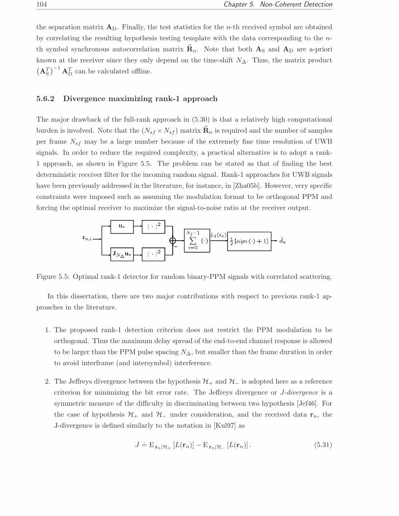
104 Chapter 5. Non-Coherent Detection
the separation matrix AD. Finally, the test statistics for the n-th received symbol are obtained
by correlating the resulting hypothesis testing template with the data corresponding to the n-
th symbol synchronous autocorrelation matrix Rn. Note that both AS and AD are a-priori
known at the receiver since they only depend on the time-shift N∆. Thus, the matrix product(AT
S
)−1AT
D can be calculated offline.
5.6.2 Divergence maximizing rank-1 approach
The major drawback of the full-rank approach in (5.30) is that a relatively high computational
burden is involved. Note that the (Nsf ×Nsf ) matrix Rn is required and the number of samples
per frame Nsf may be a large number because of the extremely fine time resolution of UWB
signals. In order to reduce the required complexity, a practical alternative is to adopt a rank-
1 approach, as shown in Figure 5.5. The problem can be stated as that of finding the best
deterministic receiver filter for the incoming random signal. Rank-1 approaches for UWB signals
have been previously addressed in the literature, for instance, in [Zha05b]. However, very specific
constraints were imposed such as assuming the modulation format to be orthogonal PPM and
forcing the optimal receiver to maximize the signal-to-noise ratio at the receiver output.
Figure 5.5: Optimal rank-1 detector for random binary-PPM signals with correlated scattering.
In this dissertation, there are two major contributions with respect to previous rank-1 ap-
proaches in the literature.
1. The proposed rank-1 detection criterion does not restrict the PPM modulation to be
orthogonal. Thus the maximum delay spread of the end-to-end channel response is allowed
to be larger than the PPM pulse spacing N∆, but smaller than the frame duration in order
to avoid interframe (and intersymbol) interference.
2. The Jeffreys divergence between the hypothesis H+ and H− is adopted here as a reference
criterion for minimizing the bit error rate. The Jeffreys divergence or J-divergence is a
symmetric measure of the difficulty in discriminating between two hypothesis [Jef46]. For
the case of hypothesis H+ and H− under consideration, and the received data rn, the
J-divergence is defined similarly to the notation in [Kul97] as
J.= E rn|H+
[L(rn)] − E rn|H−[L(rn)] . (5.31)

5.6. Optimal Receiver under the Correlated Scattering Assumption 105
An interesting property of the J-divergence measure in (5.31) is that it is closely related
with the Kullback-Leibler pseudo-distance as follows,
J = D (H+‖H−) + D (H−‖H+) (5.32)
with D (H+‖H−) the Kullback-Leibler pseudo-distance between the probability density
function for hypothesis H+ and the probability density function for hypothesis H−. That
is5,
D (H+‖H−).=
∫
rn
f (rn|H+) logf (rn|H+)
f (rn|H−)drn. (5.33)
Note that, according to the GLRT definition in (5.12), the Kullback-Leibler pseudo-
distance can also be expressed as
D (H+‖H−) =
∫
rn
f (rn|H+) log Λ (rn) drn (5.34)
=
∫
rn
f (rn|H+)L (rn) drn (5.35)
= E rn|H+[L(rn)] . (5.36)
Similarly for the converse D (H−‖H+),
D (H−‖H+) =
∫
rn
f (rn|H−) logf (rn|H−)
f (rn|H+)drn (5.37)
= −∫
rn
f (rn|H−) log Λ (rn) drn (5.38)
= −∫
rn
f (rn|H−)L (rn) drn (5.39)
= −E rn|H−[L(rn)] . (5.40)
Finally, we have that
J.= E rn|H+
[L(rn)] − E rn|H−[L(rn)] = D (H+‖H−) + D (H−‖H+) . (5.41)
With the above considerations, it seems reasonable to design the optimal low-rank detector
by selecting those eigenmodes from Cg that maximize the J-divergence. By doing so, and from
the interpretation in terms of Kullback-Leibler pseudo-distance, we are indeed maximizing the
distance between hypothesis H+ and hypothesis H−. Consequently, the substitution with the
log-GLRT test in (5.13) results in the J-divergence for the problem at hand to be given by
J ∝ Tr([
C+ − C−
] [Ern|H+
[Rn
]− Ern|H−
[Rn
]])(5.42)
= Tr([
C+ − C−
][C+ + CN − (C− + CN)]
)(5.43)
= ‖C+ − C−‖2F (5.44)
5In the formal definition of the J-divergence and the Kullback-Leibler pseudo-distance, the dependence with
the unknown waveform covariance matrix Cg is omitted for clarity.

106 Chapter 5. Non-Coherent Detection
where all the irrelevant constant terms have been omitted for simplicity.
The result in (5.44) indicates that the difficulty in discriminating between H+ and H− is
given by the distance between the corresponding signal covariance matrices {C+,C−}. This is a
very important result since it can be used to evaluate the impact of the pulse-spacing N∆ in the
discrimination between H+ and H−. An example is shown in Figure 5.6 for different channel
models of the IEEE 802.15.3a/4a standards.
1 100 200 300 400 500 600 7000
0.1
0.2
0.3
0.4
0.5
0.6
0.7
0.8
0.9
1
Time shift (samples)
Div
erge
nce
full−rank J−divergence
IEEE 802.11.15.3a CM1IEEE 802.11.15.3a CM3IEEE 802.11.15.4a CM8
Figure 5.6: Normalized J-divergence as a function of the PPM time-shift N∆ for different channel
models. Sampling time 250 ps.
The rank-1 approach aims to provide the best deterministic receiving filter that maximizes
the J-divergence in (5.44). To this end, let us express the signal covariance matrix under H+ as
C+ = UDUT , with the (Nsf×Nsf ) matrix U =[u0,u1, . . . ,uNsf−1
]containing the eigenvectors
of C+ and the diagonal matrix D = diag (λ0, λ1, . . . , λNsf−1) containing the corresponding
eigenvalues. In this way, the log-GLRT in (5.13) and the J-divergence in (5.44) can equivalently
be expressed as,
L′d(rn|Cg) =
1
Nf
d−1∑
m=0
Nf−1∑
i=0
λm
[‖uT
mrn,i‖2 − ‖uTmJT
N∆rn,i‖2
](5.45)
Jd =2
Nf
d−1∑
p=0
d−1∑
q=0
λpλq
[1 −
(uT
p JN∆uq
)2]
(5.46)
with d the dimension of the signal subspace, i.e., the number of significant eigenvalues. For the
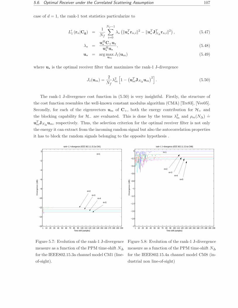
5.6. Optimal Receiver under the Correlated Scattering Assumption 107
case of d = 1, the rank-1 test statistics particularize to
L′1 (rn|Cg) =
1
Nf
Nf−1∑
i=0
λ⋆
(‖uT
⋆ rn,i‖2 − ‖uT⋆ JT
N∆rn,i‖2
), (5.47)
λ⋆ =uH
⋆ C+u⋆
uH⋆ u⋆
, (5.48)
u⋆ = arg maxum
J1(um) (5.49)
where u⋆ is the optimal receiver filter that maximizes the rank-1 J-divergence
J1(um) =2
Nfλ2
m
[1 −
(uT
mJN∆um
)2]. (5.50)
The rank-1 J-divergence cost function in (5.50) is very insightful. Firstly, the structure of
the cost function resembles the well-known constant modulus algorithm (CMA) [Tre83], [Vee05].
Secondly, for each of the eigenvectors um of C+, both the energy contribution for H+ and
the blocking capability for H− are evaluated. This is done by the terms λ2m and ρm(N∆)
.=
uTmJN∆
um, respectively. Thus, the selection criterion for the optimal receiver filter is not only
the energy it can extract from the incoming random signal but also the autocorrelation properties
it has to block the random signals belonging to the opposite hypothesis .
1 10 20 30 40 50 60 70 80 90 100 110 120 130 140 150 160 170 180 190 200−16
−14
−12
−10
−8
−6
−4
−2
0
Time shift (samples)
Div
erg
en
ce
(d
B)
rank−1 J−divergence (IEEE 802.11.15.3a CM1)
m=1
m=2
m=3 m=4
m=5
Figure 5.7: Evolution of the rank-1 J-divergence
measure as a function of the PPM time-shift N∆
for the IEEE802.15.3a channel model CM1 (line-
of-sight).
1 10 20 30 40 50 60 70 80 90 100 110 120 130 140 150 160 170 180 190 200−2
−1.8
−1.6
−1.4
−1.2
−1
−0.8
−0.6
−0.4
−0.2
0
Time shift (samples)
Div
erg
en
ce
(d
B)
rank−1 J−divergence (IEEE 802.11.15.4a CM8)
m=1
m=5
m=4 m=3
m=2
Figure 5.8: Evolution of the rank-1 J-divergence
measure as a function of the PPM time-shift N∆
for the IEEE802.15.4a channel model CM8 (in-
dustrial non line-of-sight)

108 Chapter 5. Non-Coherent Detection
5.6.3 Iterative solution for the divergence maximizing receiver filter
In this section an iterative procedure is proposed to circumvent the computationally demanding
task of the complete eigendecomposition of Cg within C+. Apart from the computational
savings, the iterative approach provides a more flexible design criterion where transitions between
different propagation scenarios can be optimally tracked with an appropriate memory factor.
This can be done by properly updating the estimated synchronous autocorrelation matrix R
and feeding this information to the iterative criterion.
In the sequel the stochastic gradient descent method is adopted for addressing the iterative
optimization in (5.49)-(5.50). The recursion is considered here to be given by
u(k+1)⋆ = u
(k)⋆ + µ [∇um log J1(um)]∣∣um=u
(k)⋆
(5.51)
∇um log J1(um) =[ (
1 − ρ2m(N∆)
)(C+ − λmI) − λmρm(N∆)JN∆
]um. (5.52)
with µ a fixed step size. Note that the gradient descent method in (5.51) is applied to the
logarithm of the rank-1 divergence cost function. By doing so, the optimal solution remains the
same but the expression for the gradient is simpler. Finally, the gradient in (5.52) is evaluated
assuming that the eigenvalue λm and the autocorrelation ρm(N∆) are defined as
λm.=
uTmC+um
uTmum
(5.53)
ρm(N∆).= uT
mJN∆um. (5.54)
In practice, an estimate for C+ can be obtained in a straightforward manner by properly zero-
padding the estimate Cg proposed in (5.9).
An example of the resulting waveform for the best deterministic rank-1 receiver filter u⋆ is
shown in Figure 5.9 for the case of the IEEE 802.15.4a CM8 channel model with a sampling
time of Ts = 0.25 ns, a PPM time-shift of N∆ = 100 samples and a frame-interval of Nsf = 1000
samples. The optimal receiving filter is shown on the bottom left hand side of Figure 5.9 whereas
the receiving filter obtained by using the gradient descent method in (5.51)-(5.52) is shown on
the top left hand side. The resulting value of the rank-1 J-divergence is also depicted on the
right hand side of Figure 5.9 as a function of the number of iterations.
It is important to remark that the proposed iterative approach resembles the well-known
Rayleigh quotient iteration (RQI) which provides the maximum eigenvalue and the correspond-
ing eigenvector of any symmetric matrix [Gol96]. The resemblance with the RQI is clear when
orthogonal PPM is considered. In that case we have ρm(n) = 0 for all m when n ≥ N∆ as a
result of the orthogonal transmission. Thus the gradient in (5.52) simplifies to
∇um log J1(um)∣∣orthogonal 2−PPM= [C+ − λmI]um (5.55)

5.6. Optimal Receiver under the Correlated Scattering Assumption 109
0 200 400 600 800 1000
−0.4
−0.3
−0.2
−0.1
0
0.1
0.2
0.3
0 200 400 600 800 1000
−0.4
−0.3
−0.2
−0.1
0
0.1
0.2
0.3
Time (samples)
Am
plit
ud
e
0 10 20 30 40 50 60 70 80 90 1000
5
10
15
20
25
30
35
40
Number of iteration (steeepest descent)
Rank−1 J−divergence
Estimated receiver filterOptimal receiver filter
Figure 5.9: Best deterministic receiver filter for the IEEE 802.15.4a CM8 channel model accord-
ing to the proposed iterative rank-1 J-divergence optimization. The estimated filter at the end
of 100 iterations is shown in the top left hand side corner whereas the exact filter is shown in
the bottom left hand side corner.
which coincides with the gradient of the RQI [Gol96]. Therefore, the best deterministic receiver
filter for orthogonal PPM corresponds to the well-known result of being the maximum eigenvec-
tor of Cg (i.e. C+). This solution is also found to provide the maximum signal-to-noise ratio at
the receiver output. For non-orthogonal PPM, however, the solution is not trivial and it must
be determined based on the maximization of the rank-1 J-divergence cost function proposed in
(5.50).
Finally, note that the proposed rank-1 receiver in Figure 5.5 can be extended to the case where
a set of d0 > 1 eigenmodes are considered. In that situation the receiver architecture can be
generalized to the rank-d0 architecture depicted in Figure 5.10. The receiver filters u⋆|d in Figure
5.10 are obtained in a sequential manner starting from u⋆|d=1 and using (5.51). Once u⋆|d=1 is
obtained, the covariance matrix C+ must be updated as follows, C+|d = C+|d−1 − u⋆|d−1uT⋆|d−1
and the iterative procedure in (5.51) must be started again with the new covariance matrix.
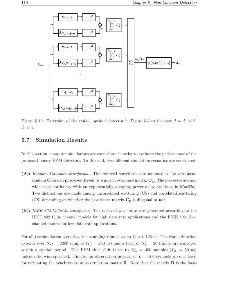
110 Chapter 5. Non-Coherent Detection
Figure 5.10: Extension of the rank-1 optimal detector in Figure 5.5 to the case d = d0 with
d0 > 1.
5.7 Simulation Results
In this section, computer simulations are carried out in order to evaluate the performance of the
proposed binary-PPM detectors. To this end, two different simulation scenarios are considered:
(A): Random Gaussian waveforms. The received waveforms are assumed to be zero-mean
random Gaussian processes driven by a given covariance matrix Cg. The processes are non
wide-sense stationary with an exponentially decaying power delay profile as in [Cas02a].
Two distinctions are made among uncorrelated scattering (US) and correlated scattering
(CS) depending on whether the covariance matrix Cg is diagonal or not.
(B): IEEE 802.15.3a/4a waveforms. The received waveforms are generated according to the
IEEE 802.15.3a channel models for high data rate applications and the IEEE 802.15.4a
channel models for low data rate applications.
For all the simulation scenarios, the sampling time is set to Ts = 0.125 ns. The frame duration
extends over Nsf = 2000 samples (Tf = 250 ns) and a total of Nf = 20 frames are conveyed
within a symbol period. The PPM time shift is set to N∆ = 400 samples (T∆ = 50 ns)
unless otherwise specified. Finally, an observation interval of L = 500 symbols is considered
for estimating the synchronous autocorrelation matrix R. Note that the matrix R is the basis

5.7. Simulation Results 111
for estimating the covariance matrices Cg or C+ as indicated in Section 5.3. The performance
results for the proposed receivers are compared with the performance of the well-known energy-
detector receiver (ED) [Rab04a], [Wei04] which is a simple but suboptimal receiver that assumes
the power delay profile of the channel to be constant. For the simulation results with the ED
receiver, the integration length is set to be equal to the time-shift N∆.
0 200 400 600 800 1000 1200 1400 1600 1800 2000−10
−5
0
5
10
Time (samples)
Am
plit
ud
e
0 200 400 600 800 1000 1200 1400 1600 1800 2000−10
−5
0
5
10
Time (samples)
Am
plit
ud
e
Uncorrelated samples
Correlated samples
Figure 5.11: 1000 realizations of the Gaussian random received waveforms with uncorrelated
samples (top) and correlated samples (bottom). The power delay profile is exponentially decay-
ing with an average delay spread of 100 samples. For correlated samples, the time-lags of the
autocorrelation are also exponentially decaying with an average spread of 200 samples.
5.7.1 Simulation results for random Gaussian waveforms
Experiment 1: Random waveforms with US. In this experiment the received waveforms are mod-
eled as zero-mean Gaussian random processes with uncorrelated samples. The power-delay pro-
file is exponentially decaying with an average delay spread of 100 samples (12.5 ns). A total of
1000 waveforms are depicted at the top of Figure 5.11 for illustrating the shape of the received
waveforms. For this simulation set-up, two different PPM time-shifts are considered: N∆ = 30
samples (3.75 ns) and N∆ = 400 samples (50 ns).
The receiver performance is analyzed in terms of bit error rate (BER) and it is shown in
Figure 5.12 as a function of the energy-per-symbol to noise spectral density Es/N0. As it
is expected, the full-rank detector based on (5.30) and the PDP detector based on (5.26) do

112 Chapter 5. Non-Coherent Detection
coincide. Note that the PDP detector just considers the main diagonal of the covariance matrix
Cg whereas the full-rank detector estimates the whole covariance matrix Cg and compresses this
information into the likelihood ratio test statistics. However, in the presence of US scattering,
Cg is diagonal and thus the full-rank detector is indeed a PDP detector.
6 8 10 12 14 16 18 20 22 24 26 2810
−4
10−3
10−2
10−1
100
Es/N
0 (dB)
BE
R
N∆=30 samples
ED detectorPDP detectorrank−1 detectorfull−rank detectorTR signal + TR detectorTR signal + full−rank detector
6 8 10 12 14 16 18 20 22 24 26 2810
−4
10−3
10−2
10−1
100
Es/N
0 (dB)
BE
R
N∆=400 samples
Figure 5.12: BER performance for random Gaussian UWB signals with uncorrelated scattering.
Contrary to the full-rank and the PDP detectors, the rank-1 detector provides the worst
performance. This is because the uncorrelateness of the received samples expands the number
of significant eigenmodes in the covariance matrix Cg. As a result, the contribution of a rank-1
approximation is almost negligible compared with the large amount of significant eigenvalues.
Finally, the results in Figure 5.12 also incorporate the performance of a transmitted-reference
(TR) scheme where an unmodulated pulse is transmitted prior to each data modulated pulse.
In order to model rapid time variations of the propagation environment, the end-to-end channel
response is assumed to change from frame to frame. As shown in Figure 5.12, this causes a severe
degradation of the TR scheme. The reason is that each unmodulated pulse can only be used for
one modulated pulse and thus, no coherent integration can be performed across multiple frames
to combat the severe noise contribution. However, a significant improvement can be obtained
when the TR signal is processed by the full rank detector. In that way, the optimal receiver for
time-varying channels is adopted and there is just about 3 dB of performance loss due to the
transmission of unmodulated pulses.
Experiment 2: Random waveforms with correlated samples. In this experiment, the received
waveforms are modeled as Gaussian random processes with correlated samples. The power delay
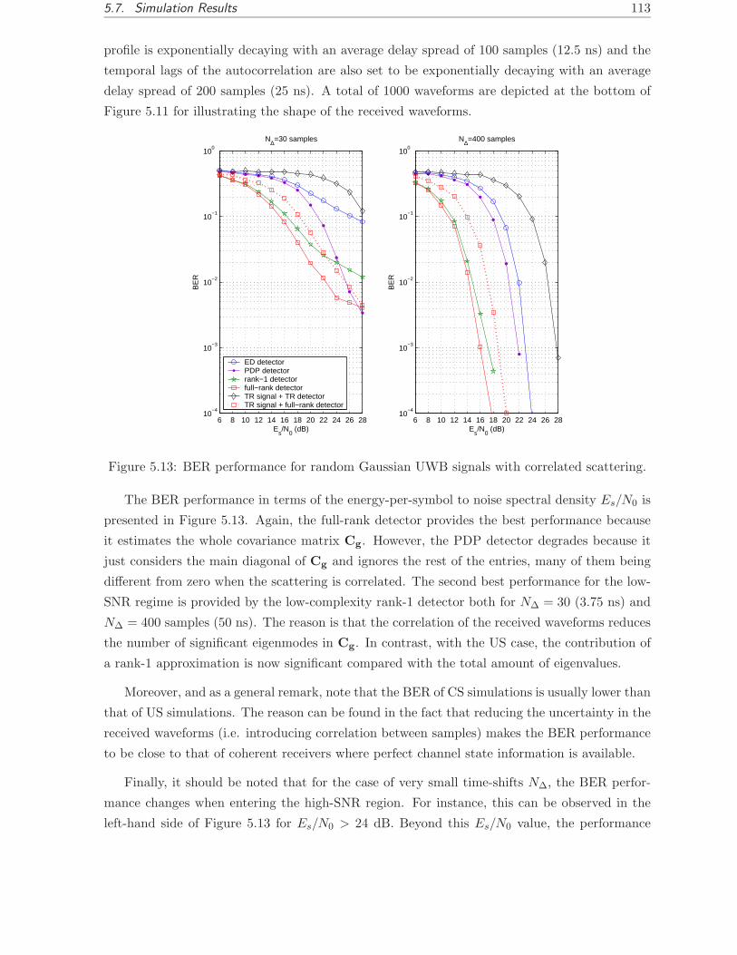
5.7. Simulation Results 113
profile is exponentially decaying with an average delay spread of 100 samples (12.5 ns) and the
temporal lags of the autocorrelation are also set to be exponentially decaying with an average
delay spread of 200 samples (25 ns). A total of 1000 waveforms are depicted at the bottom of
Figure 5.11 for illustrating the shape of the received waveforms.
6 8 10 12 14 16 18 20 22 24 26 2810
−4
10−3
10−2
10−1
100
Es/N
0 (dB)
BE
R
N∆=30 samples
ED detectorPDP detectorrank−1 detectorfull−rank detectorTR signal + TR detectorTR signal + full−rank detector
6 8 10 12 14 16 18 20 22 24 26 2810
−4
10−3
10−2
10−1
100
Es/N
0 (dB)
BE
R
N∆=400 samples
Figure 5.13: BER performance for random Gaussian UWB signals with correlated scattering.
The BER performance in terms of the energy-per-symbol to noise spectral density Es/N0 is
presented in Figure 5.13. Again, the full-rank detector provides the best performance because
it estimates the whole covariance matrix Cg. However, the PDP detector degrades because it
just considers the main diagonal of Cg and ignores the rest of the entries, many of them being
different from zero when the scattering is correlated. The second best performance for the low-
SNR regime is provided by the low-complexity rank-1 detector both for N∆ = 30 (3.75 ns) and
N∆ = 400 samples (50 ns). The reason is that the correlation of the received waveforms reduces
the number of significant eigenmodes in Cg. In contrast, with the US case, the contribution of
a rank-1 approximation is now significant compared with the total amount of eigenvalues.
Moreover, and as a general remark, note that the BER of CS simulations is usually lower than
that of US simulations. The reason can be found in the fact that reducing the uncertainty in the
received waveforms (i.e. introducing correlation between samples) makes the BER performance
to be close to that of coherent receivers where perfect channel state information is available.
Finally, it should be noted that for the case of very small time-shifts N∆, the BER perfor-
mance changes when entering the high-SNR region. For instance, this can be observed in the
left-hand side of Figure 5.13 for Es/N0 > 24 dB. Beyond this Es/N0 value, the performance
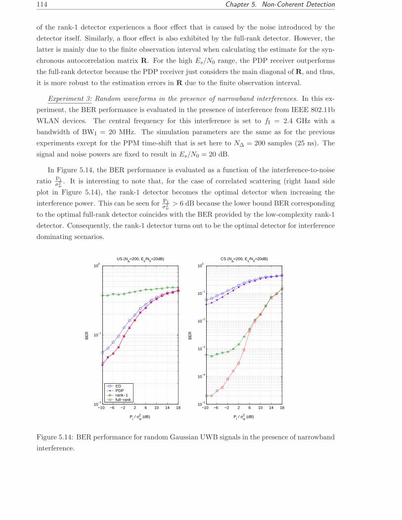
114 Chapter 5. Non-Coherent Detection
of the rank-1 detector experiences a floor effect that is caused by the noise introduced by the
detector itself. Similarly, a floor effect is also exhibited by the full-rank detector. However, the
latter is mainly due to the finite observation interval when calculating the estimate for the syn-
chronous autocorrelation matrix R. For the high Es/N0 range, the PDP receiver outperforms
the full-rank detector because the PDP receiver just considers the main diagonal of R, and thus,
it is more robust to the estimation errors in R due to the finite observation interval.
Experiment 3: Random waveforms in the presence of narrowband interferences. In this ex-
periment, the BER performance is evaluated in the presence of interference from IEEE 802.11b
WLAN devices. The central frequency for this interference is set to fI = 2.4 GHz with a
bandwidth of BWI = 20 MHz. The simulation parameters are the same as for the previous
experiments except for the PPM time-shift that is set here to N∆ = 200 samples (25 ns). The
signal and noise powers are fixed to result in Es/N0 = 20 dB.
In Figure 5.14, the BER performance is evaluated as a function of the interference-to-noise
ratio PIσ2
w. It is interesting to note that, for the case of correlated scattering (right hand side
plot in Figure 5.14), the rank-1 detector becomes the optimal detector when increasing the
interference power. This can be seen for PIσ2
w> 6 dB because the lower bound BER corresponding
to the optimal full-rank detector coincides with the BER provided by the low-complexity rank-1
detector. Consequently, the rank-1 detector turns out to be the optimal detector for interference
dominating scenarios.
−10 −6 −2 2 6 10 14 1810
−2
10−1
100
PI / σ
w2 (dB)
BE
R
US (N∆=200, Es/N
0=20dB)
−10 −6 −2 2 6 10 14 1810
−5
10−4
10−3
10−2
10−1
100
PI / σ
w2 (dB)
BE
R
CS (N∆=200, Es/N
0=20dB)
EDPDPrank−1full−rank
Figure 5.14: BER performance for random Gaussian UWB signals in the presence of narrowband
interference.
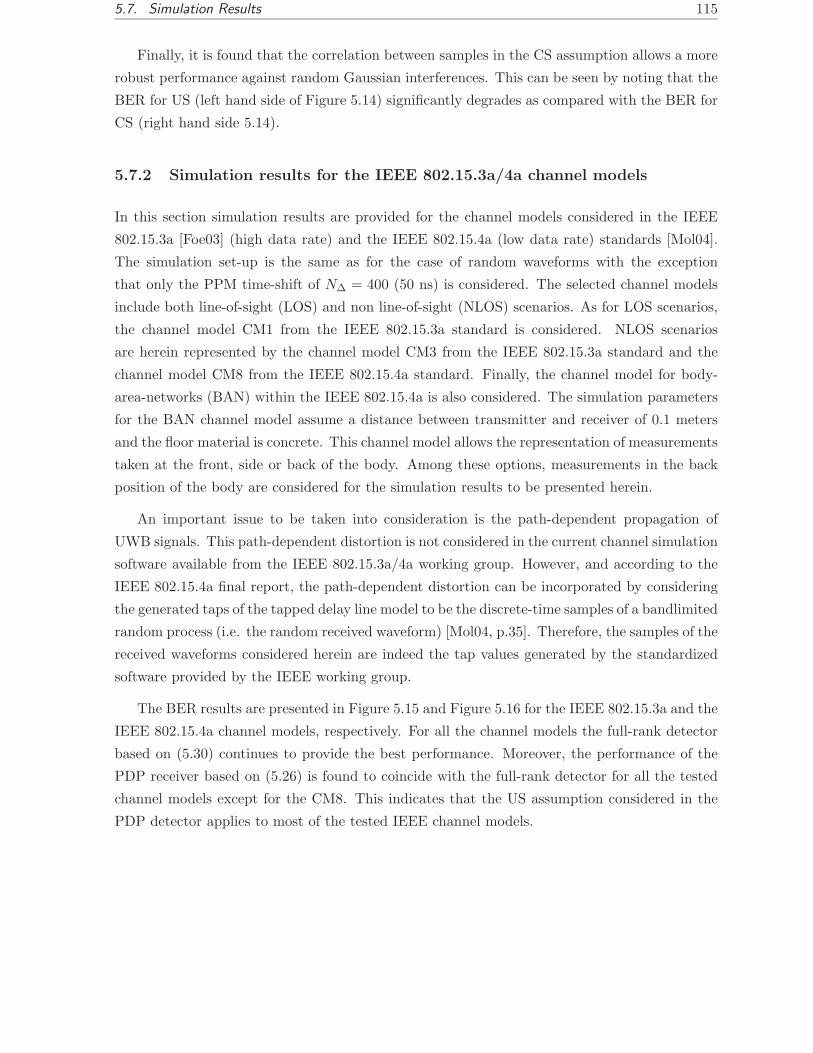
5.7. Simulation Results 115
Finally, it is found that the correlation between samples in the CS assumption allows a more
robust performance against random Gaussian interferences. This can be seen by noting that the
BER for US (left hand side of Figure 5.14) significantly degrades as compared with the BER for
CS (right hand side 5.14).
5.7.2 Simulation results for the IEEE 802.15.3a/4a channel models
In this section simulation results are provided for the channel models considered in the IEEE
802.15.3a [Foe03] (high data rate) and the IEEE 802.15.4a (low data rate) standards [Mol04].
The simulation set-up is the same as for the case of random waveforms with the exception
that only the PPM time-shift of N∆ = 400 (50 ns) is considered. The selected channel models
include both line-of-sight (LOS) and non line-of-sight (NLOS) scenarios. As for LOS scenarios,
the channel model CM1 from the IEEE 802.15.3a standard is considered. NLOS scenarios
are herein represented by the channel model CM3 from the IEEE 802.15.3a standard and the
channel model CM8 from the IEEE 802.15.4a standard. Finally, the channel model for body-
area-networks (BAN) within the IEEE 802.15.4a is also considered. The simulation parameters
for the BAN channel model assume a distance between transmitter and receiver of 0.1 meters
and the floor material is concrete. This channel model allows the representation of measurements
taken at the front, side or back of the body. Among these options, measurements in the back
position of the body are considered for the simulation results to be presented herein.
An important issue to be taken into consideration is the path-dependent propagation of
UWB signals. This path-dependent distortion is not considered in the current channel simulation
software available from the IEEE 802.15.3a/4a working group. However, and according to the
IEEE 802.15.4a final report, the path-dependent distortion can be incorporated by considering
the generated taps of the tapped delay line model to be the discrete-time samples of a bandlimited
random process (i.e. the random received waveform) [Mol04, p.35]. Therefore, the samples of the
received waveforms considered herein are indeed the tap values generated by the standardized
software provided by the IEEE working group.
The BER results are presented in Figure 5.15 and Figure 5.16 for the IEEE 802.15.3a and the
IEEE 802.15.4a channel models, respectively. For all the channel models the full-rank detector
based on (5.30) continues to provide the best performance. Moreover, the performance of the
PDP receiver based on (5.26) is found to coincide with the full-rank detector for all the tested
channel models except for the CM8. This indicates that the US assumption considered in the
PDP detector applies to most of the tested IEEE channel models.
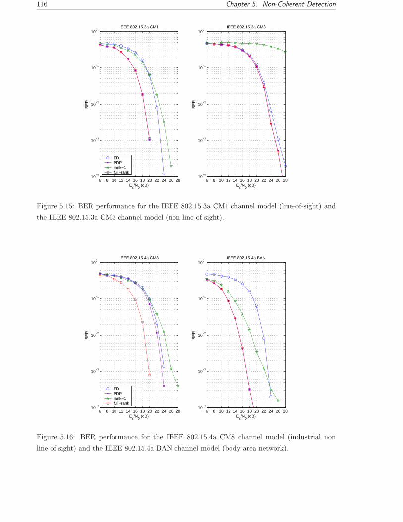
116 Chapter 5. Non-Coherent Detection
6 8 10 12 14 16 18 20 22 24 26 2810
−4
10−3
10−2
10−1
100
Es/N
0 (dB)
BE
R
IEEE 802.15.3a CM1
EDPDPrank−1full−rank
6 8 10 12 14 16 18 20 22 24 26 2810
−4
10−3
10−2
10−1
100
Es/N
0 (dB)
BE
R
IEEE 802.15.3a CM3
Figure 5.15: BER performance for the IEEE 802.15.3a CM1 channel model (line-of-sight) and
the IEEE 802.15.3a CM3 channel model (non line-of-sight).
6 8 10 12 14 16 18 20 22 24 26 2810
−4
10−3
10−2
10−1
100
Es/N
0 (dB)
BE
R
IEEE 802.15.4a CM8
EDPDPrank−1full−rank
6 8 10 12 14 16 18 20 22 24 26 2810
−4
10−3
10−2
10−1
100
Es/N
0 (dB)
BE
R
IEEE 802.15.4a BAN
Figure 5.16: BER performance for the IEEE 802.15.4a CM8 channel model (industrial non
line-of-sight) and the IEEE 802.15.4a BAN channel model (body area network).

5.8. Conclusions 117
Related with the above remark, note that the rank-1 detector usually provides the worst
performance except for the BAN channel. This is due to the fact that the rank-1 detector is
devoted to propagation environments where the amplitudes of the received samples (not the
absolute values) are correlated and thus, the channel energy is only spread over a small number
of eigenmodes.
The requirement of correlated received samples is not fulfilled in most of the considered
channel models, as indicated in [Saa04], [Men05]. Thus the performance of the rank-1 detector
seriously degrades. For the BAN channel, however, the reasonable performance of the rank-1
detector is in line with the correlated scattering results found in [For06].
5.8 Conclusions
The optimal framework for the symbol decision problem of binary-PPM with random UWB
signals has been presented. The optimal symbol decision statistics are provided and the rela-
tionship with previous contributions in the current literature has been revised. Two different
analyses for the symbol decision problem have been presented depending on whether the am-
plitudes of the received waveforms are correlated or not. The correlated scenario is of special
interest since it is found to allow a low cost implementation of the optimal symbol detector. In
this sense, an iterative algorithm is proposed for the design of the optimal receiver filter which
is based on information-theoretic criteria and allow us to minimize the bit error probability.

118 Chapter 5. Non-Coherent Detection
Appendix 5.A Derivation of the Low-SNR Generalized Likelihood
Ratio Test
The GLRT provides the optimal decision rule for deciding between the hypothesis H+ : dn = 1
and H− : dn = 0 based on the probability density function of the received data conditioned on
the hypothesis to be tested. According to the channel model in Section 5.2, the conditioned
probability density function for the n-th received symbol under H+ is given by the multivariate
Gaussian probability density function,
f (rn|H+;Cg) =
Nf−1∏
i=0
1
(2π)Nsf /2 det1/2 (C+ + CN)exp
(−1
2rTn,i (C+ + CN)−1 rn,i
)(5.56)
with C+.= ΠCgΠ
T the covariance matrix for the signal received under H+ and CN.= σ2
wI +
CI the covariance matrix for the Gaussian contribution of both the thermal noise and the
narrowband interference.
Similarly to (5.56), the conditioned probability density function under the hypothesis H− is
found by substituting C+ in (5.56) with C−.= JN∆
ΠCgΠTJN∆
. When both f(rn|H+;Cg) and
f(rn|H−;Cg) are available, the GLRT results in
Λ(rn|Cg) =det1/2 (C− + CN)
det1/2 (C+ + CN)
Nf−1∏
i=0
exp(−1
2rTn,i (C+ + CN)−1 rn,i
)
exp(−1
2rTn,i (C− + CN)−1 rn,i
) . (5.57)
The GLRT in (5.57) can be significantly simplified when both the noise and the interference are
high-power sources compared with the UWB transmitter. The following assumptions can be
done:
(AS1) Assumption 1:det (C− + CN)
det (C+ + CN)≈ 1. (5.58)
Proof. Let us first expand the determinant det (C+ + CN) as follows,
det (C+ + CN) = det(C+ + σ2
wI + CI
)= det
(σ2
w
[σ−2
w C+ + I + σ−2w CI
])(5.59)
= σ2Nsfw det
(σ−2
w C+ + I + σ−2w CI
). (5.60)
Since the noise is considered a high-power source compared to the UWB signal, it is reasonable
to assume that σ−2w C+ ≈ 0. Note that the same approximation cannot be applied to the
term σ−2w CI since both the noise and the interference may have powers on the same order.
Consequently,
det (C+ + CN) ≈ σ2Nsfw det
(I + σ−2
w CI
). (5.61)
The key point is to notice that the approximation in (5.61) does not depend on the sig-
nal covariance matrix C+. The same conclusion applies when expanding the determinant
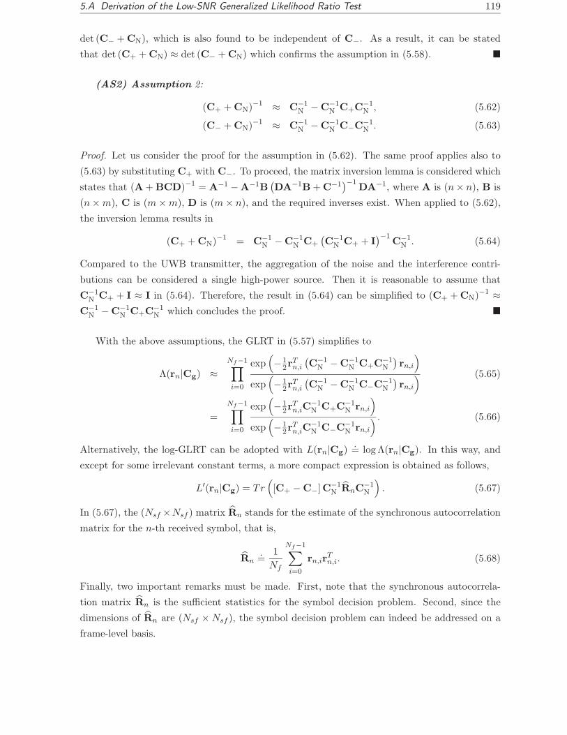
5.A Derivation of the Low-SNR Generalized Likelihood Ratio Test 119
det (C− + CN), which is also found to be independent of C−. As a result, it can be stated
that det (C+ + CN) ≈ det (C− + CN) which confirms the assumption in (5.58). ¥
(AS2) Assumption 2:
(C+ + CN)−1 ≈ C−1N − C−1
N C+C−1N , (5.62)
(C− + CN)−1 ≈ C−1N − C−1
N C−C−1N . (5.63)
Proof. Let us consider the proof for the assumption in (5.62). The same proof applies also to
(5.63) by substituting C+ with C−. To proceed, the matrix inversion lemma is considered which
states that (A + BCD)−1 = A−1 −A−1B(DA−1B + C−1
)−1DA−1, where A is (n× n), B is
(n × m), C is (m × m), D is (m × n), and the required inverses exist. When applied to (5.62),
the inversion lemma results in
(C+ + CN)−1 = C−1N − C−1
N C+
(C−1
N C+ + I)−1
C−1N . (5.64)
Compared to the UWB transmitter, the aggregation of the noise and the interference contri-
butions can be considered a single high-power source. Then it is reasonable to assume that
C−1N C+ + I ≈ I in (5.64). Therefore, the result in (5.64) can be simplified to (C+ + CN)−1 ≈
C−1N − C−1
N C+C−1N which concludes the proof. ¥
With the above assumptions, the GLRT in (5.57) simplifies to
Λ(rn|Cg) ≈Nf−1∏
i=0
exp(−1
2rTn,i
(C−1
N − C−1N C+C−1
N
)rn,i
)
exp(−1
2rTn,i
(C−1
N − C−1N C−C−1
N
)rn,i
) (5.65)
=
Nf−1∏
i=0
exp(−1
2rTn,iC
−1N C+C−1
N rn,i
)
exp(−1
2rTn,iC
−1N C−C−1
N rn,i
) . (5.66)
Alternatively, the log-GLRT can be adopted with L(rn|Cg).= log Λ(rn|Cg). In this way, and
except for some irrelevant constant terms, a more compact expression is obtained as follows,
L′(rn|Cg) = Tr([C+ − C−]C−1
N RnC−1N
). (5.67)
In (5.67), the (Nsf ×Nsf ) matrix Rn stands for the estimate of the synchronous autocorrelation
matrix for the n-th received symbol, that is,
Rn.=
1
Nf
Nf−1∑
i=0
rn,irTn,i. (5.68)
Finally, two important remarks must be made. First, note that the synchronous autocorrela-
tion matrix Rn is the sufficient statistics for the symbol decision problem. Second, since the
dimensions of Rn are (Nsf × Nsf ), the symbol decision problem can indeed be addressed on a
frame-level basis.
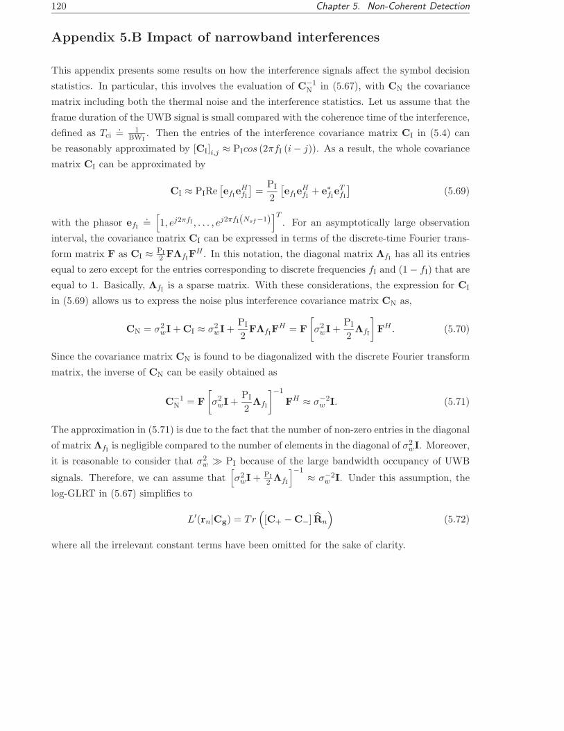
120 Chapter 5. Non-Coherent Detection
Appendix 5.B Impact of narrowband interferences
This appendix presents some results on how the interference signals affect the symbol decision
statistics. In particular, this involves the evaluation of C−1N in (5.67), with CN the covariance
matrix including both the thermal noise and the interference statistics. Let us assume that the
frame duration of the UWB signal is small compared with the coherence time of the interference,
defined as Tci.= 1
BWI. Then the entries of the interference covariance matrix CI in (5.4) can
be reasonably approximated by [CI]i,j ≈ PIcos (2πfI (i − j)). As a result, the whole covariance
matrix CI can be approximated by
CI ≈ PIRe[efI
eHfI
]=
PI
2
[efI
eHfI
+ e∗fIeT
fI
](5.69)
with the phasor efI
.=
[1, ej2πfI , . . . , ej2πfI(Nsf−1)
]T. For an asymptotically large observation
interval, the covariance matrix CI can be expressed in terms of the discrete-time Fourier trans-
form matrix F as CI ≈ PI2 FΛfI
FH . In this notation, the diagonal matrix ΛfIhas all its entries
equal to zero except for the entries corresponding to discrete frequencies fI and (1 − fI) that are
equal to 1. Basically, ΛfIis a sparse matrix. With these considerations, the expression for CI
in (5.69) allows us to express the noise plus interference covariance matrix CN as,
CN = σ2wI + CI ≈ σ2
wI +PI
2FΛfI
FH = F
[σ2
wI +PI
2ΛfI
]FH . (5.70)
Since the covariance matrix CN is found to be diagonalized with the discrete Fourier transform
matrix, the inverse of CN can be easily obtained as
C−1N = F
[σ2
wI +PI
2ΛfI
]−1
FH ≈ σ−2w I. (5.71)
The approximation in (5.71) is due to the fact that the number of non-zero entries in the diagonal
of matrix ΛfIis negligible compared to the number of elements in the diagonal of σ2
wI. Moreover,
it is reasonable to consider that σ2w ≫ PI because of the large bandwidth occupancy of UWB
signals. Therefore, we can assume that[σ2
wI + PI2 ΛfI
]−1≈ σ−2
w I. Under this assumption, the
log-GLRT in (5.67) simplifies to
L′(rn|Cg) = Tr([C+ − C−] Rn
)(5.72)
where all the irrelevant constant terms have been omitted for the sake of clarity.
Chapter 6
Non-Coherent Frame-Timing
Acquisition
6.1 Introduction
The attractive features of UWB technology are based on its particular transmission format based
on the emission of extremely-short and low-power pulses. However, although UWB technology
has been around since the 1960s, it has been mainly used in the past for low data rate and
non-communications applications because of the great difficulty in efficiently handling such a
stream of sub-nanosecond pulses. It has not been until the recent years that the implementation
of high data rate and reliable UWB communication systems has become feasible.
Nowadays, one of the most challenging issues is still concerned with the synchronization of
UWB signals [Yan04b]. In particular, timing recovery becomes a critical issue because of the
extremely-short time duration of the transmitted pulses. For both coherent and non-coherent
receivers, timing recovery is required at the frame level to determine the starting point of each
information-bearing symbol. For coherent receivers, timing recovery is also required at the
pulse level to find where the pulse is located within the frame period. In that way, the optimal
sampling time instant can be selected when correlating the received signal with the local replica
of the received pulses [Win97], [Mir01]. In any case, proper alignment of the received signal is
found to be essential for reliable communication.
In this chapter the problem of timing acquisition for UWB signals focuses on three major
aspects:
• Non-coherent receiver. The non-coherent approach is inherited from Chapter 5 and it is
motivated by the complex propagation physics of UWB signals that make fast and accurate
channel estimation a challenging and computationally demanding task [Cra02], [Qiu02],
121
122 Chapter 6. Non-Coherent Frame-Timing Acquisition
[Qiu05]. In these circumstances it is reasonable to assume that neither the transmitted
pulse nor the channel response are known at the receiver. For this reason, the received
waveform is considered here to be an unknown parameter in the mathematical formulation.
Thus, the proposed techniques in this chapter can be thought of as waveform-independent
techniques. By waveform-independent we mean that no effort is placed on estimating the
channel response.
• Nondata-aided synchronization. The timing recovery is addressed under a nondata-
aided perspective. In that way, the transmitted symbols are assumed to be unknown.
Since no pilot symbols are required, nondata-aided techniques can operate with any piece of
modulated data without any prior prealignment. In addition, by adopting a nondata-aided
strategy, the effective transmitted throughput is maximized and the mean transmitted
power is minimized.
• Frame-level timing. Similarly to traditional spread-spectrum communication systems,
the timing recovery for UWB signals can be decomposed into two stages. Firstly, frame-
level timing acquisition (i.e. coarse acquisition). Secondly, pulse-level timing acquisition
(i.e. fine acquisition). This chapter focuses on the first stage of the timing recovery, that
is, frame-timing acquisition. The second stage is not considered since the notion of fine
timing error is always related to some reference pulse. Since a non-coherent receiver is
adopted and thus, the received waveform is assumed to be unknown, the fine timing error
is undefined and it is considered to be part of the shape of the unknown waveform.
Many contributions in the recent literature do address the problem of timing recovery for
UWB signals. However, some kind of a priori knowledge is usually assumed at the receiver
such as training symbols (e.g. [Yan03a], [Tia05d], [Tia05e], [Car06b]), or perfect channel state
information. As for the latter, the frame-timing acquisition problem is often addressed in a
rather heuristic or ad-hoc manner by adopting some kind of correlator-based receiver. That
is, coherent receivers are adopted and a replica of the received waveform is assumed to be
available at the receiver for matched filtering [Win98], [Zha03],[Bla03]. Usually, the output
statistics are processed either by exploiting the cyclostationary properties of the transmitted
signal [Tia02], by adopting search algorithms [Gez02], [Hom02] or by using parallel architectures
[Lov02]. Interestingly, significant efforts are also being placed on addressing the acquisition
problem under a more rigorous approach. To this end, the maximum likelihood formulation has
already been proposed, for instance, in some valuable contributions such as the ones in [Lot00]
and [Car04a].
Regarding the non-coherent approach to the problem, it is important to mention that recent
contributions in the field of UWB timing acquisition are aware of the necessity to make the
acquisition process a waveform-independent procedure. This is especially important in low

6.2. Optimal Frame-Timing Acquisition in the low-SNR Regime 123
cost sensor networks, where energy collection is usually adopted as a simple and effective way
to implement low-cost non-coherent receivers [Che05]. Another possible alternative to avoid
channel estimation is to use a piece of the received signal as the correlating pattern. This is the
idea behind the concept of dirty template which is presented in [Yan04a], [Yan05] and related
to transmitted reference approaches in [Rus64], [Hoc02], [Cha03]. However, the main drawback
of this approach is that a relatively high signal-to-noise ratio (SNR) is required for obtaining a
valid timing estimate when dealing with modulated data. Other approaches can also be found
in the literature such as transmitting nonzero mean amplitude modulating symbols [Luo05]. In
this way, the received signal can be averaged on a symbol-by-symbol basis so as to obtain the
received waveform at the expense of a degradation in spectral efficiency.
The work to be presented herein differs from previous contributions related to the timing
acquisition of UWB signals. The reason is that the problem is addressed in a systematic and ana-
lytic manner under the well-known unconditional maximum likelihood criterion [Ott93], [Vaz00].
By adopting a general nondata-aided approach, it is shown that optimal frame-level timing esti-
mation is possible when neither the transmitted symbols nor the received waveform are known
at the receiver. Indeed, the resulting estimator is reminiscent of the energy detection approach
adopted in many radar signal detection techniques [Rab04a]. Finally, it is worth noting that
the proposed method is not restricted to the modulation format of UWB signals and it can be
applied to other spread spectrum communication systems.
The chapter is structured as follows. The optimal frame-timing acquisition approach is
presented in Section 6.2 within the framework of unconditional maximum likelihood estima-
tion. Because of the particular working conditions of UWB communication systems, particular
emphasis is placed on the acquisition problem for the low-SNR regime. The derivation of the
optimal frame-timing acquisition method is introduced in Section 6.2.4, the proposed implemen-
tation is presented in Section 6.2.6 and Section 6.2.7, and some simulation results are analyzed
in Section 6.2.8. Moreover, a low complexity implementation of the proposed frame-timing ac-
quisition approach is presented in Section 6.3 as a solution to a model-order detection problem.
The proposed low-cost implementation is discussed in Section 6.3.4 and simulation results are
also enclosed in Section 6.3.5. Finally, conclusions are drawn in Section 6.4.
6.2 Optimal Frame-Timing Acquisition in the low-SNR Regime
6.2.1 Signal Model in Scalar Notation
The signal model to be considered in this chapter assumes the transmission of ultra-short pulses
with pulse-position modulation (PPM), pulse-amplitude modulation (PAM), or possibly both,

124 Chapter 6. Non-Coherent Frame-Timing Acquisition
the so-called amplitude-pulse-position modulation (APPM)1. The discrete-time representation
of the received signal is given by
r(k) =+∞∑
n=−∞
sngT (k − dnN∆ − nNss − τ) + w(k) (6.1)
with dn the pulse-position modulating symbols, N∆ the PPM time-shift in samples, Nss the
number of samples per symbol (i.e. the symbol period), τ the symbol timing error and w(k)
the Gaussian contribution from the thermal noise and possible multiple user interference. The
amplitude values represented by sn have two different goals depending on whether amplitude
modulation is implemented or not. On the one hand, sn represents the amplitude modulating
information-bearing symbols when PAM or APPM modulation is considered. On the other
hand, sn = {−1, +1} represents a simple symbol-by-symbol polarity randomization code for
avoiding the existence of spectral lines caused by PPM modulation [Nak03]. Thus, the sign of
sn is ignored by non-coherent PPM receivers since it does not bear any information.
The major difference between the signal model in (6.1) and the one adopted in Chapter 5
is the adoption of the template waveform gT (k) as the basis for the frame-timing acquisition
problem. The template waveform collects the set of Nf repeated pulses that represent the
transmission of a single information-bearing symbol, and it is given by
gT (k).=
Nf−1∑
i=0
g(k − iNsf − uiNsc) (6.2)
with Nsf the number of samples per frame (i.e. the frame duration) and ui = {0, 1, . . . , Nc − 1}the time-hopping (TH) code with time resolution Nsc samples2. The length of the template
waveform is Nss = NfNsf and the frame duration is assumed to be large enough so as to
avoid interframe interference due to the channel delay spread, pulse-position modulation and
time-hopping. Similarly to [Yan04a], the TH code is assumed to be periodic within the symbol
duration. In contrast with Chapter 5, the received waveforms g(k) in (6.2) are assumed to
be unknown but not time-varying for the sake of simplicity. However, time-varying random
waveforms can indeed be supported by the proposed timing acquisition technique as long as the
coherence time is larger than the symbol period.
Finally, the symbol timing error τ is constrained within τ ∈ [0, Nss), and it can be decom-
posed as
τ = NǫNsf + ǫ (6.3)
1The combination of both PPM and PAM is an approach that has also been adopted in [Li00], [Zha05a], or in
[Tan05a] for application to transmitted-reference systems.2The problem of TH code acquisition is not considered here since it is a whole problem itself and shares
many similarities with the problem of code acquisition for traditional spread-spectrum communication systems.
However, some references about this topic can be found in [Hom02], [Gez02] and [Reg05], among many others.
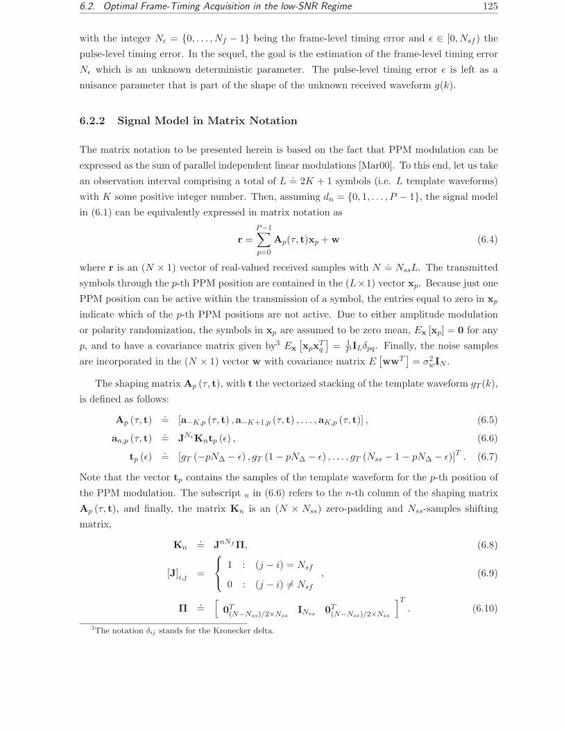
6.2. Optimal Frame-Timing Acquisition in the low-SNR Regime 125
with the integer Nǫ = {0, . . . , Nf − 1} being the frame-level timing error and ǫ ∈ [0, Nsf ) the
pulse-level timing error. In the sequel, the goal is the estimation of the frame-level timing error
Nǫ which is an unknown deterministic parameter. The pulse-level timing error ǫ is left as a
nuisance parameter that is part of the shape of the unknown received waveform g(k).
6.2.2 Signal Model in Matrix Notation
The matrix notation to be presented herein is based on the fact that PPM modulation can be
expressed as the sum of parallel independent linear modulations [Mar00]. To this end, let us take
an observation interval comprising a total of L.= 2K + 1 symbols (i.e. L template waveforms)
with K some positive integer number. Then, assuming dn = {0, 1, . . . , P − 1}, the signal model
in (6.1) can be equivalently expressed in matrix notation as
r =P−1∑
p=0
Ap(τ, t)xp + w (6.4)
where r is an (N × 1) vector of real-valued received samples with N.= NssL. The transmitted
symbols through the p-th PPM position are contained in the (L×1) vector xp. Because just one
PPM position can be active within the transmission of a symbol, the entries equal to zero in xp
indicate which of the p-th PPM positions are not active. Due to either amplitude modulation
or polarity randomization, the symbols in xp are assumed to be zero mean, Ex [xp] = 0 for any
p, and to have a covariance matrix given by3 Ex
[xpx
Tq
]= 1
P ILδpq. Finally, the noise samples
are incorporated in the (N × 1) vector w with covariance matrix E[wwT
]= σ2
wIN .
The shaping matrix Ap (τ, t), with t the vectorized stacking of the template waveform gT (k),
is defined as follows:
Ap (τ, t).= [a−K,p (τ, t) ,a−K+1,p (τ, t) , . . . ,aK,p (τ, t)] , (6.5)
an,p (τ, t).= JNǫKntp (ǫ) , (6.6)
tp (ǫ).= [gT (−pN∆ − ǫ) , gT (1 − pN∆ − ǫ) , . . . , gT (Nss − 1 − pN∆ − ǫ)]T . (6.7)
Note that the vector tp contains the samples of the template waveform for the p-th position of
the PPM modulation. The subscript n in (6.6) refers to the n-th column of the shaping matrix
Ap (τ, t), and finally, the matrix Kn is an (N × Nss) zero-padding and Nss-samples shifting
matrix,
Kn.= JnNf Π, (6.8)
[J]i,j =
1 : (j − i) = Nsf
0 : (j − i) 6= Nsf
, (6.9)
Π.=
[0T
(N−Nss)/2×NssINss 0T
(N−Nss)/2×Nss
]T
. (6.10)
3The notation δij stands for the Kronecker delta.
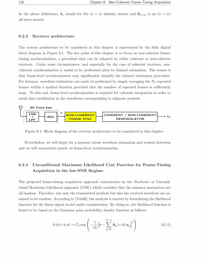
126 Chapter 6. Non-Coherent Frame-Timing Acquisition
In the above definitions, In stands for the (n × n) identity matrix and 0n×m is an (n × m)
all-zeros matrix.
6.2.3 Receiver architecture
The system architecture to be considered in this chapter is represented by the fully digital
block diagram in Figure 6.1. The key point of this chapter is to focus on non-coherent frame-
timing synchronization, a procedure that can be adopted by either coherent or non-coherent
receivers. Under some circumstances, and especially for the case of coherent receivers, non-
coherent synchronization is useful to be performed prior to channel estimation. The reason is
that frame-level synchronization may significantly simplify the channel estimation procedure.
For instance, waveform estimation can easily be performed by simply averaging the Nf repeated
frames within a symbol duration provided that the number of repeated frames is sufficiently
large. To this end, frame-level synchronization is required for coherent integration in order to
avoid data modulation in the waveforms corresponding to adjacent symbols.
Figure 6.1: Block diagram of the receiver architecture to be considered in this chapter.
Nevertheless, we will forget for a moment about waveform estimation and symbol detection
and we will concentrate purely on frame-level synchronization.
6.2.4 Unconditional Maximum Likelihood Cost Function for Frame-Timing
Acquisition in the low-SNR Regime
The proposed frame-timing acquisition approach concentrates on the Stochastic or Uncondi-
tional Maximum Likelihood approach (UML) which considers that the nuisance parameters are
all random. Therefore, not only the transmitted symbols but also the received waveform are as-
sumed to be random. According to [Vaz00], the analysis is started by formulating the likelihood
function for the linear signal model under consideration. By doing so, the likelihood function is
found to be based on the Gaussian noise probability density function as follows:
Λ (r|τ ; t;x) = C0 exp
− 1
σ2w
∥∥∥r −P−1∑
p=0
Ap (τ, t)xp
∥∥∥2
(6.11)

6.2. Optimal Frame-Timing Acquisition in the low-SNR Regime 127
with C0 an irrelevant positive constant. By expanding the quadratic norm in (6.11) and taking
into consideration just those terms which depend on the parameters of interest, we have
Λ (r|τ ; t;x) = C1 exp
(2
σ2w
χ (r; τ ; t;x)
), (6.12)
χ (r; τ ; t;x).=
P−1∑
p=0
xTp AT
p r − 1
2
P−1∑
p=0
P−1∑
q=0
xTp AT
p Aqxq, (6.13)
with C1 = C0 exp(−rT r/σ2
w
)and where the dependence of Ap on (τ ; t) is omitted for the sake
of simplicity. Assuming the SNR to be sufficiently low, the likelihood function presented so far
can be importantly simplified. This is the reason why the low-SNR assumption is traditionally
adopted in the derivation of many blind synchronizers within the ML estimation framework
[Men97]. For the case of UWB signals, the application of the low-SNR assumption is completely
justified by the extremely low power radiating conditions of the UWB transmission. A low-SNR
analysis not only provides an easier manipulation of the likelihood function but also a realistic
approach to the real working conditions. Under the low-SNR assumption, the likelihood function
in (6.12)-(6.13) can be approximated by its second order Taylor series expansion as follows,
Λ (r|τ ; t;x) ≈ C1
[1 +
2
σ2w
χ (r; τ ; t;x) +2
σ4w
χ2 (r; τ ; t;x)
]. (6.14)
In order to obtain a likelihood function which does not depend on neither the transmitted
symbols nor the received waveform, the next step is to eliminate the dependence on the set of
nuisance parameters {t;x} from (6.14).
6.2.4.1 Marginal likelihood function with respect of the transmitted symbols
The dependence on the transmitted symbols can be avoided by adopting the marginal likelihood
function
Λ (r|τ ; t) = Ex [Λ (r|τ ; t;x)] . (6.15)
Therefore, and according to the results in Appendix 6.A and Appendix 6.B, it is found that
Ex [χ (r; τ ; t;x)] = γa (t) , (6.16)
Ex
[χ2 (r; τ ; t;x)
]=
P−1∑
p=0
rTApATp r + γb (t) , (6.17)
with {γa (t) , γb (t)} two constant terms with respect to the symbol timing error τ but with
dependence on the template waveform t. With these considerations, the likelihood function in
(6.15) can be expressed as
Λ (r|τ ; t) ≈ C1
1 +
2γa (t)
σ2w
+2γb (t)
σ4w
+2
σ4w
P−1∑
p=0
rTApATp r
. (6.18)

128 Chapter 6. Non-Coherent Frame-Timing Acquisition
Next, the expression of the shaping matrix Ap in (6.5)-(6.7) can be substituted into (6.18)
resulting in
Λ (r|τ ; t) ≈ C1
1 +
2γa (t)
σ2w
+2γb (t)
σ4w
+2
σ4w
P−1∑
p=0
K∑
n=−K
Tr(tp (ǫ) tT
p (ǫ)KTnJ−NǫrrTJNǫKn
)
= C1
[1 +
2γa (t)
σ2w
+2γb (t)
σ4w
+2LP
σ4w
Tr (T(ǫ)R(Nǫ))
], (6.19)
with
T (ǫ).=
1
P
P−1∑
p=0
tp (ǫ) tp (ǫ) = Ex
[t (ǫ) tT (ǫ)
], (6.20)
R (Nǫ) =K∑
n=−K
KTnJ−NǫrrTJNǫKn. (6.21)
Note that R(Nǫ) is the (Nss × Nss) synchronous autocorrelation matrix of the received signal
when a time shift correction of NǫNsf samples is applied on it. In this sense, the time-shifted
synchronous autocorrelation matrix is defined as
R (m).= lim
L→∞
1
L
L−1∑
n=0
rn (m) rTn (m) (6.22)
with
rn (m).= [r(nNss + mNsf ), r(nNss + mNsf + 1), . . . , r(nNss + mNsf + Nss − 1)]T . (6.23)
6.2.4.2 Marginal likelihood function with respect of the template waveform
In the current approach to the timing estimation problem for UWB signals, the received template
waveform is assumed to be unknown. For this reason, the template waveform is considered a
nuisance parameter in the subsequent formulation. Similarly, the residual pulse-level timing
error ǫ can also be considered a nuisance parameter as well. This is similar to what happens in
traditional timing estimation for non-coherent receivers at the output of an unknown frequency-
selective channel [Git92, p.434]. In that case, the pulse-level timing error is not properly defined
because it is always related to some reference pulse. Since the reference pulse is not available
in non-coherent receivers, the pulse-level timing error is unknown and it can be incorporated as
part of the shape of the unknown received waveform.
Since both the received waveform and the pulse-level timing error are assumed to be nuisance
parameters, the marginal likelihood function from (6.15) depends only on the frame-level timing
error Nǫ,
Et,ǫ [Λ (r|τ ; t)] = Λ (r|Nǫ) . (6.24)
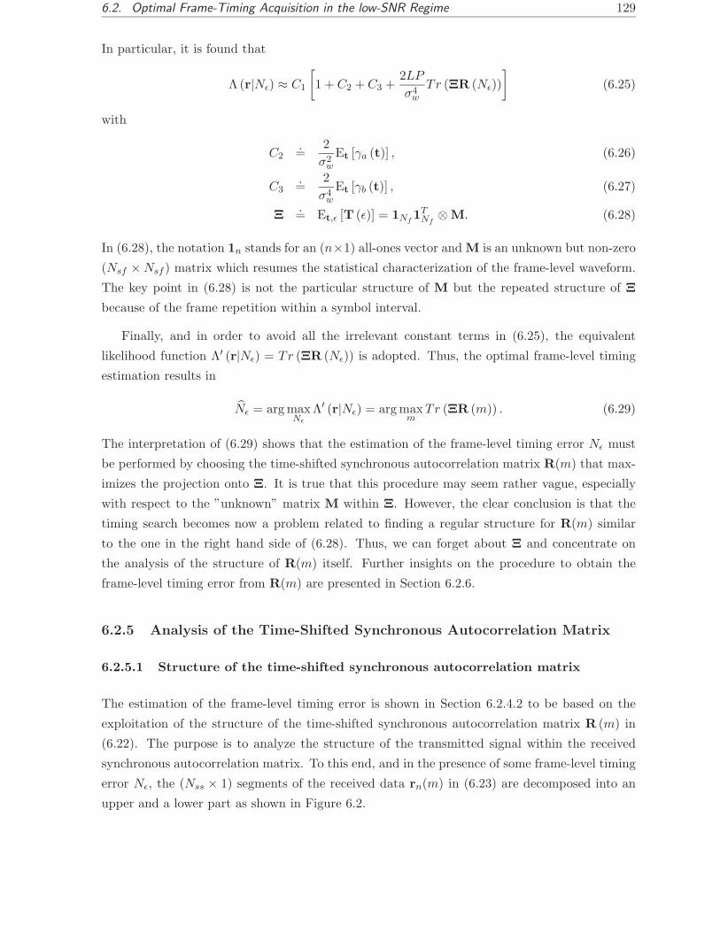
6.2. Optimal Frame-Timing Acquisition in the low-SNR Regime 129
In particular, it is found that
Λ (r|Nǫ) ≈ C1
[1 + C2 + C3 +
2LP
σ4w
Tr (ΞR (Nǫ))
](6.25)
with
C2.=
2
σ2w
Et [γa (t)] , (6.26)
C3.=
2
σ4w
Et [γb (t)] , (6.27)
Ξ.= Et,ǫ [T (ǫ)] = 1Nf
1TNf
⊗ M. (6.28)
In (6.28), the notation 1n stands for an (n×1) all-ones vector and M is an unknown but non-zero
(Nsf × Nsf ) matrix which resumes the statistical characterization of the frame-level waveform.
The key point in (6.28) is not the particular structure of M but the repeated structure of Ξ
because of the frame repetition within a symbol interval.
Finally, and in order to avoid all the irrelevant constant terms in (6.25), the equivalent
likelihood function Λ′ (r|Nǫ) = Tr (ΞR (Nǫ)) is adopted. Thus, the optimal frame-level timing
estimation results in
Nǫ = arg maxNǫ
Λ′ (r|Nǫ) = arg maxm
Tr (ΞR (m)) . (6.29)
The interpretation of (6.29) shows that the estimation of the frame-level timing error Nǫ must
be performed by choosing the time-shifted synchronous autocorrelation matrix R(m) that max-
imizes the projection onto Ξ. It is true that this procedure may seem rather vague, especially
with respect to the ”unknown” matrix M within Ξ. However, the clear conclusion is that the
timing search becomes now a problem related to finding a regular structure for R(m) similar
to the one in the right hand side of (6.28). Thus, we can forget about Ξ and concentrate on
the analysis of the structure of R(m) itself. Further insights on the procedure to obtain the
frame-level timing error from R(m) are presented in Section 6.2.6.
6.2.5 Analysis of the Time-Shifted Synchronous Autocorrelation Matrix
6.2.5.1 Structure of the time-shifted synchronous autocorrelation matrix
The estimation of the frame-level timing error is shown in Section 6.2.4.2 to be based on the
exploitation of the structure of the time-shifted synchronous autocorrelation matrix R (m) in
(6.22). The purpose is to analyze the structure of the transmitted signal within the received
synchronous autocorrelation matrix. To this end, and in the presence of some frame-level timing
error Nǫ, the (Nss × 1) segments of the received data rn(m) in (6.23) are decomposed into an
upper and a lower part as shown in Figure 6.2.

130 Chapter 6. Non-Coherent Frame-Timing Acquisition
Figure 6.2: Structure of the received signal when some time delay is present. Note that each
vector of received samples rn is composed by an upper and lower part, b(n) and a(n) respectively,
which correspond to segments of two consecutive transmitted templates.
More specifically, the lower part of rn corresponds to the transmission of the current symbol.
This lower part is indicated by an ((Nss − (Nǫ − m)Nsf ) × 1) vector of samples an. Similarly,
the upper part of rn corresponds to the transmission of the previous symbol. This upper part is
indicated by an ((Nǫ − m)Nsf × 1) vector of samples bn−1. According to these considerations,
rn(m) =
sn−1bn−1
snan
+ wn (m) (6.30)
with
wn (m).= [w(nNss + mNsf ), w(nNss + mNsf + 1), . . . , w(nNss + mNsf + Nss − 1)]T . (6.31)
Note that the amplitude modulating symbols {sn−1, sn} are explicitly indicated in (6.30) whereas
the possible position modulating symbols are implicitly incorporated within bn−1 and an. More-
over, note that for m = Nǫ, the received signal is synchronized and thus rn(Nǫ) = snan + wn
according to (6.30).
Then, by taking into consideration that E [sisj ] = δij , the time-shifted synchronous autocor-
relation matrix results in
R (m)|Nǫ=i =
Tb(i) 0P (m;i)×Q(m;i)
0Q(m;i)×P (m;i) Ta(i)
+ σ2
wINss (6.32)
with P (m; i).= (i − m) Nsf and Q(m; i)
.= (Nss − (i − m) Nsf ). Matrices Ta and Tb come from
the definition of T in (6.20) but in its block-partitioned form,
T =
Ta(i) TT
c (i)
Tc(i) Tb(i)
(6.33)
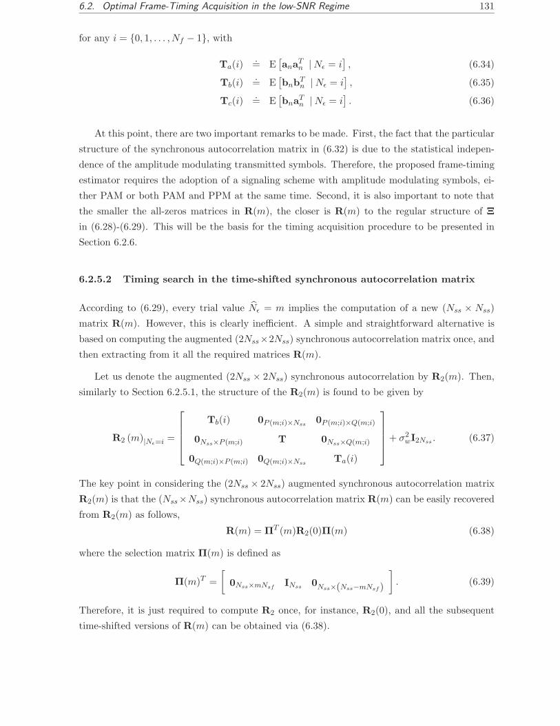
6.2. Optimal Frame-Timing Acquisition in the low-SNR Regime 131
for any i = {0, 1, . . . , Nf − 1}, with
Ta(i).= E
[ana
Tn | Nǫ = i
], (6.34)
Tb(i).= E
[bnb
Tn | Nǫ = i
], (6.35)
Tc(i).= E
[bna
Tn | Nǫ = i
]. (6.36)
At this point, there are two important remarks to be made. First, the fact that the particular
structure of the synchronous autocorrelation matrix in (6.32) is due to the statistical indepen-
dence of the amplitude modulating transmitted symbols. Therefore, the proposed frame-timing
estimator requires the adoption of a signaling scheme with amplitude modulating symbols, ei-
ther PAM or both PAM and PPM at the same time. Second, it is also important to note that
the smaller the all-zeros matrices in R(m), the closer is R(m) to the regular structure of Ξ
in (6.28)-(6.29). This will be the basis for the timing acquisition procedure to be presented in
Section 6.2.6.
6.2.5.2 Timing search in the time-shifted synchronous autocorrelation matrix
According to (6.29), every trial value Nǫ = m implies the computation of a new (Nss × Nss)
matrix R(m). However, this is clearly inefficient. A simple and straightforward alternative is
based on computing the augmented (2Nss×2Nss) synchronous autocorrelation matrix once, and
then extracting from it all the required matrices R(m).
Let us denote the augmented (2Nss × 2Nss) synchronous autocorrelation by R2(m). Then,
similarly to Section 6.2.5.1, the structure of the R2(m) is found to be given by
R2 (m)|Nǫ=i =
Tb(i) 0P (m;i)×Nss0P (m;i)×Q(m;i)
0Nss×P (m;i) T 0Nss×Q(m;i)
0Q(m;i)×P (m;i) 0Q(m;i)×NssTa(i)
+ σ2
wI2Nss . (6.37)
The key point in considering the (2Nss × 2Nss) augmented synchronous autocorrelation matrix
R2(m) is that the (Nss×Nss) synchronous autocorrelation matrix R(m) can be easily recovered
from R2(m) as follows,
R(m) = ΠT (m)R2(0)Π(m) (6.38)
where the selection matrix Π(m) is defined as
Π(m)T =
[0Nss×mNsf
INss 0Nss×(Nss−mNsf)
]. (6.39)
Therefore, it is just required to compute R2 once, for instance, R2(0), and all the subsequent
time-shifted versions of R(m) can be obtained via (6.38).
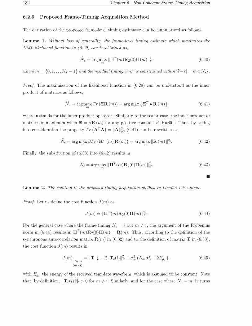
132 Chapter 6. Non-Coherent Frame-Timing Acquisition
6.2.6 Proposed Frame-Timing Acquisition Method
The derivation of the proposed frame-level timing estimator can be summarized as follows.
Lemma 1. Without loss of generality, the frame-level timing estimate which maximizes the
UML likelihood function in (6.29) can be obtained as,
Nǫ = arg maxm
‖ΠT (m)R2(0)Π(m)‖2F (6.40)
where m = {0, 1, . . . Nf − 1} and the residual timing error is constrained within |τ−τ | = ǫ < Nsf .
Proof. The maximization of the likelihood function in (6.29) can be understood as the inner
product of matrices as follows,
Nǫ = arg maxm
Tr (ΞR (m)) = arg maxm
{ΞT • R (m)
}(6.41)
where • stands for the inner product operator. Similarly to the scalar case, the inner product of
matrices is maximum when Ξ = βR (m) for any positive constant β [Har00]. Thus, by taking
into consideration the property Tr(ATA
)= ‖A‖2
F , (6.41) can be rewritten as,
Nǫ = arg maxm
βTr(RT (m)R (m)
)= arg max
m‖R (m) ‖2
F . (6.42)
Finally, the substitution of (6.38) into (6.42) results in
Nǫ = arg maxm
‖ΠT (m)R2(0)Π(m)‖2F . (6.43)
¥
Lemma 2. The solution to the proposed timing acquisition method in Lemma 1 is unique.
Proof. Let us define the cost function J(m) as
J(m).= ‖ΠT (m)R2(0)Π(m)‖2
F . (6.44)
For the general case where the frame-timing Nǫ = i but m 6= i, the argument of the Frobenius
norm in (6.44) results in ΠT (m)R2(0)Π(m) = R(m). Thus, according to the definition of the
synchronous autocorrelation matrix R(m) in (6.32) and to the definition of matrix T in (6.33),
the cost function J(m) results in
J(m) ∣∣Nǫ=i
(m6=i)
= ‖T‖2F − 2‖Tc(i)‖2
F + σ2w
(Nssσ
2w + 2EgT
), (6.45)
with EgTthe energy of the received template waveform, which is assumed to be constant. Note
that, by definition, ‖Tc(i)‖2F > 0 for m 6= i. Similarly, and for the case where Nǫ = m, it turns

6.2. Optimal Frame-Timing Acquisition in the low-SNR Regime 133
out that ΠT (m)R2(0)Π(m) = R(Nǫ) = T + σ2wINss . Therefore, the cost function J(m) results
in
J(m)|Nǫ=m = ‖T‖2F + σ2
w
(Nssσ
2w + 2EgT
)(6.46)
From the results in (6.45) and (6.46), it is found that
J(m)|Nǫ=m > J(m)|Nǫ 6=m (6.47)
which guarantees the uniqueness of the solution to (6.40). ¥
It is important to note that the proposed frame-level timing estimation method in (6.40) is
based on a frame-level search over the synchronous autocorrelation matrix of the received signal.
This can be shown in Figure 6.3 both when timing error is absent or present.
Figure 6.3: Illustration of the sliding matrix ΠT (m)R2Π(m) (thick line) when R2 is computed
from received samples with perfectly acquired timing (left) or with some timing error τ (right).
From the above considerations, the synchronous autocorrelation matrix becomes the suffi-
cient statistics for the problem at hand. Contrary to [Yan04a], where a non-coherent integration
of the noise is performed, an important advantage of the proposed method is that a coherent
integration is addressed in the off-diagonal entries of the synchronous autocorrelation matrix.
As a result, the proposed method is expected to be more robust to low signal-to-noise ratio
scenarios than the one in [Yan04a].
6.2.7 Algorithm Implementation
An important issue when implementing the proposed method in Section 6.2.6 is to realize that
it is not necessary to compute the Frobenius norm for every trial value m in (6.40). The reason
is that, from Nǫ = m − 1 to Nǫ = m, most of the entries in the associated Frobenius norm are
the same, so they can be reused as indicated in Figure 6.4.
As a result, the Frobenius norm for Nǫ = m can be computed from the Frobenius norm for
Nǫ = m − 1, resulting in the procedure shown in Table 6.1. In the algorithm description of

134 Chapter 6. Non-Coherent Frame-Timing Acquisition
Figure 6.4: When the sliding matrix ΠT (m − 1)R2Π(m − 1) is shifted to ΠT (m)R2Π(m),
the backward and the forward regions appear which allow an optimized computation of the
Frobenius norm for ΠT (m)R2Π(m).
Table 6.1, the Matlabr notation R2 (a : b, c : d) has been used to denote the elements of matrix
R2 contained within the a-th to b-th rows and within the c-th to d-th columns, with a < b and
c < d. That is, the entries contained within the rectangular region which is bounded by the
upper left hand corner (a, c) and the lower right hand corner (b, d).
Regarding the computational complexity, most of the required computational burden of the
proposed algorithm is due to the computation of the (2Nss ×2Nss) synchronous autocorrelation
matrix in Step 1 of Table 6.1. In particular, the overall complexity of the proposed algorithm
can be roughly approximated to 8N2f LN2
sf flops (floating point operations). Note that the
complexity of the proposed algorithm is quadratic on the number of samples per frame Nsf . This
is in contrast with the timing acquisition algorithm in [Yan04a] which is adopted for comparison
in the simulation results of Section 6.2.8. The algorithm in [Yan04a] is quite simple and it
just requires approximately N2f LNsf flops. Thus, it has a linear dependence on the number of
samples per frame Nsf in contrast with the quadratic dependence of the proposed algorithm.
However, the increase in complexity for the proposed method comes at the expense of a
better performance. This can be observed in Section 6.2.8 where the proposed frame-timing
acquisition method is found to clearly outperform the one in [Yan04a] for the low signal-to-noise
ratio scenarios typically encountered in UWB communication systems.
6.2.8 Simulation Results
In this section, computer simulations are carried out to compare the performance of the proposed
frame-timing acquisition method with existing techniques in the literature. To this end, only
binary PAM modulation is considered for the sake of simplicity and two distinct simulation
scenarios are evaluated:
(A): Random Gaussian waveforms. The received waveforms are considered to be zero-mean
random Gaussian processes under the uncorrelated scattering (US) assumption. The re-
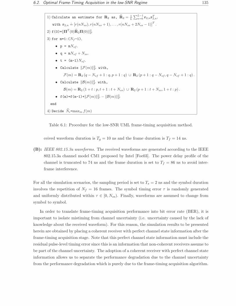
6.2. Optimal Frame-Timing Acquisition in the low-SNR Regime 135
1) Calculate an estimate for R2 as, R2 = 1L
∑L−1n=0 r2,nrT
2,n,
with r2,n.= [r(nNss), r(nNss + 1), . . . , r(nNss + 2Nss − 1)]
T.
2) f(0)=‖ΠT (0)R2Π(0)‖2F
3) for m=1:(Nf-1),
• p = mNsf .
• q = mNsf + Nss.
• t = (m-1)Nsf .
• Calculate ‖F(m)‖2F with,
F(m) = R2 (q − Nsf + 1 : q, p + 1 : q) ∪ R2 (p + 1 : q − Nsf , q − Nsf + 1 : q) .
• Calculate ‖B(m)‖2F with,
B(m) = R2 (1 + t : p, t + 1 : t + Nss) ∪ R2 (p + 1 : t + Nss, 1 + t : p) .
• f(m)=f(m-1)+‖F(m)‖2F − ‖B(m)‖2
F
end
4) Decide Nǫ=maxm f(m)
Table 6.1: Procedure for the low-SNR UML frame-timing acquisition method.
ceived waveform duration is Tg = 10 ns and the frame duration is Tf = 14 ns.
(B): IEEE 802.15.3a waveforms. The received waveforms are generated according to the IEEE
802.15.3a channel model CM1 proposed by Intel [Foe03]. The power delay profile of the
channel is truncated to 74 ns and the frame duration is set to Tf = 86 ns to avoid inter-
frame interference.
For all the simulation scenarios, the sampling period is set to Ts = 2 ns and the symbol duration
involves the repetition of Nf = 16 frames. The symbol timing error τ is randomly generated
and uniformly distributed within τ ∈ [0, Nss). Finally, waveforms are assumed to change from
symbol to symbol.
In order to translate frame-timing acquisition performance into bit error rate (BER), it is
important to isolate mistiming from channel uncertainty (i.e. uncertainty caused by the lack of
knowledge about the received waveform). For this reason, the simulation results to be presented
herein are obtained by placing a coherent receiver with perfect channel state information after the
frame-timing acquisition stage. Note that this perfect channel state information must include the
residual pulse-level timing error since this is an information that non-coherent receivers assume to
be part of the channel uncertainty. The adoption of a coherent receiver with perfect channel state
information allows us to separate the performance degradation due to the channel uncertainty
from the performance degradation which is purely due to the frame-timing acquisition algorithm.

136 Chapter 6. Non-Coherent Frame-Timing Acquisition
Finally, the results of the method proposed in Section 6.2.6 and Section 6.2.7 are compared
with the popular dirty template (DT) method proposed in [Yan04a].
6.2.8.1 Simulation results for random Gaussian waveforms
Experiment 1: BER Performance as a function of Es/N0. Figure 6.5 shows the BER results
for an observation interval of L = 100 symbols. Note that almost an error-free performance
in terms of BER is experienced for Es/N0 > 5 dB, which is indeed a really low Es/N0 value.
This is in contrast with the dirty template (DT) method, which requires a significantly higher
Es/N0 for reliable frame-timing acquisition. As it was already mentioned, the poor low-SNR
performance of the DT is caused by the non-coherent integration of the noise when evaluating
the DT cost function in [Yan04a, Eq. (14)]. In that sense, the advantage of the proposed
method is that a coherent integration of the noise terms is addressed in the off-diagonal entries
of the synchronous autocorrelation matrix. As it is well-known in statistical estimation theory,
the noise contribution in coherent integration converges faster to zero than when non-coherent
integration is performed [Kay98, p. 251]. As a result, the proposed method is found to be more
robust to low-SNR scenarios than the DT.
Experiment 2: Probability of correct frame acquisition. The results in Figure 6.6 show the
probability of correct frame acquisition as a function of the observation interval L in symbols.
The observation interval is important for the proposed method in the sense that enough data
must be processed so as to obtain a reasonable estimate for the synchronous autocorrelation
matrix of the received signals, which is the sufficient statistics for the problem at hand. For
the proposed method, the simulation results indicate that the probability of correct acquisition
rapidly improves as the observation interval increases. As a result, almost an error-free perfor-
mance is achieved for L > 80 symbols at Es/N0 = 7 dB whereas the DT method fails 50 % of
the times for the same working conditions.

6.2. Optimal Frame-Timing Acquisition in the low-SNR Regime 137
0 1 2 3 4 5 6 7 8 9 10 1110
−6
10−5
10−4
10−3
10−2
10−1
100
Es/N
0 (dB)
BE
R
Perfect timing acq.Without timing acq.Dirty templateProposed method
Figure 6.5: BER due to mistiming for an observation interval comprising L = 100 symbols with
random Gaussian waveforms.
20 40 60 80 100 120 140 160 180 200 220 240 260 280 3000.1
0.2
0.3
0.4
0.5
0.6
0.7
0.8
0.9
1
L (symbols)
Pro
b. C
orre
ct A
cqui
sitio
n
Dirty templateProposed method
Es/N
0=8dB
Es/N
0=7dB
Es/N
0=6dB
Es/N
0=8dB
Es/N
0=7dB
Es/N
0=6dB
Figure 6.6: Probability of correct frame acquisition as a function of the observation interval L
with random Gaussian waveforms.
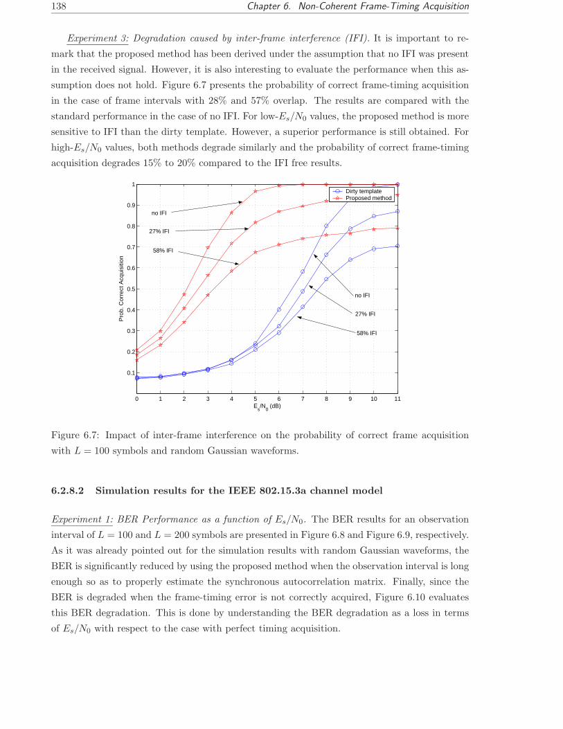
138 Chapter 6. Non-Coherent Frame-Timing Acquisition
Experiment 3: Degradation caused by inter-frame interference (IFI). It is important to re-
mark that the proposed method has been derived under the assumption that no IFI was present
in the received signal. However, it is also interesting to evaluate the performance when this as-
sumption does not hold. Figure 6.7 presents the probability of correct frame-timing acquisition
in the case of frame intervals with 28% and 57% overlap. The results are compared with the
standard performance in the case of no IFI. For low-Es/N0 values, the proposed method is more
sensitive to IFI than the dirty template. However, a superior performance is still obtained. For
high-Es/N0 values, both methods degrade similarly and the probability of correct frame-timing
acquisition degrades 15% to 20% compared to the IFI free results.
0 1 2 3 4 5 6 7 8 9 10 11
0.1
0.2
0.3
0.4
0.5
0.6
0.7
0.8
0.9
1
Es/N
0 (dB)
Pro
b. C
orre
ct A
cqui
sitio
n
Dirty templateProposed method
no IFI
27% IFI
58% IFI
58% IFI
27% IFI
no IFI
Figure 6.7: Impact of inter-frame interference on the probability of correct frame acquisition
with L = 100 symbols and random Gaussian waveforms.
6.2.8.2 Simulation results for the IEEE 802.15.3a channel model
Experiment 1: BER Performance as a function of Es/N0. The BER results for an observation
interval of L = 100 and L = 200 symbols are presented in Figure 6.8 and Figure 6.9, respectively.
As it was already pointed out for the simulation results with random Gaussian waveforms, the
BER is significantly reduced by using the proposed method when the observation interval is long
enough so as to properly estimate the synchronous autocorrelation matrix. Finally, since the
BER is degraded when the frame-timing error is not correctly acquired, Figure 6.10 evaluates
this BER degradation. This is done by understanding the BER degradation as a loss in terms
of Es/N0 with respect to the case with perfect timing acquisition.

6.2. Optimal Frame-Timing Acquisition in the low-SNR Regime 139
0 1 2 3 4 5 6 7 8 9 10 11 1210
−7
10−6
10−5
10−4
10−3
10−2
10−1
100
Es/N
0 (dB)
BE
R
Perfect timing acq.Without timing acq.Dirty templateProposed method
Figure 6.8: BER due to mistiming for an observation interval comprising L = 100 symbols with
channel model CM1 from IEEE 802.15.3a.
0 1 2 3 4 5 6 7 8 9 10 11 1210
−7
10−6
10−5
10−4
10−3
10−2
10−1
100
Es/N
0 (dB)
BE
R
Perfect timing acq.Without timing acq.Dirty templateProposed method
Figure 6.9: BER due to mistiming for an observation interval comprising L = 200 symbols with
channel model CM1 from IEEE 802.15.3a.

140 Chapter 6. Non-Coherent Frame-Timing Acquisition
0 1 2 3 4 5 6 7 8 9 10 110
1
2
3
4
5
6
7
8
9
Es/N
0 (dB)
ES/N
0 loss
(dB
)
Dirty templateProposed method
L=100
L=200
L=300
L=100
L=200
L=300
Figure 6.10: Es/N0 loss (dB) due to mistiming with respect to perfect frame acquisition for
channel CM1 from IEEE 802.15.3a.
Experiment 2: Probability of correct frame acquisition. Figure 6.11 depicts the probability of
correct frame-timing acquisition as a function of Es/N0. As for the case with random Gaussian
waveforms, the proposed method is found to provide a significantly higher probability of correct
frame-timing acquisition than the dirty template with the same simulation parameters. For the
same number of transmitted symbols L, the coherent integration of the noise allows the proposed
method to provide a more robust behavior in the low-SNR regime.
Moreover, the gain when increasing the observation interval is more significant in the pro-
posed method. For instance, for all the working conditions in Figure 6.11, the most significant
improvement in probability of correct frame acquisition is experienced at Es/N0 = 6 dB when
increasing the observation interval from L = 100 to L = 200 for the proposed method. In this
case, the probability of correct acquisition moves from 0.47 to 0.82 (almost improves 100%). In
contrast, the most significant improvement for the DT method is at Es/N0 = 10 dB (4 dB later
than for the proposed method) where the probability of correct frame acquisition moves from
0.44 to 0.65 (just 50%).
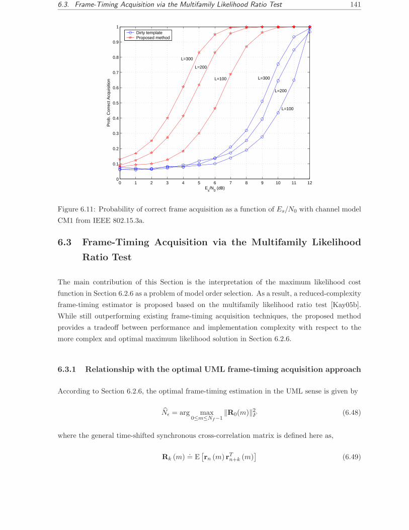
6.3. Frame-Timing Acquisition via the Multifamily Likelihood Ratio Test 141
0 1 2 3 4 5 6 7 8 9 10 11 120
0.1
0.2
0.3
0.4
0.5
0.6
0.7
0.8
0.9
1
Es/N
0 (dB)
Pro
b. C
orre
ct A
cqui
sitio
n
Dirty templateProposed method
L=300
L=200
L=100
L=100
L=200
L=300
Figure 6.11: Probability of correct frame acquisition as a function of Es/N0 with channel model
CM1 from IEEE 802.15.3a.
6.3 Frame-Timing Acquisition via the Multifamily Likelihood
Ratio Test
The main contribution of this Section is the interpretation of the maximum likelihood cost
function in Section 6.2.6 as a problem of model order selection. As a result, a reduced-complexity
frame-timing estimator is proposed based on the multifamily likelihood ratio test [Kay05b].
While still outperforming existing frame-timing acquisition techniques, the proposed method
provides a tradeoff between performance and implementation complexity with respect to the
more complex and optimal maximum likelihood solution in Section 6.2.6.
6.3.1 Relationship with the optimal UML frame-timing acquisition approach
According to Section 6.2.6, the optimal frame-timing estimation in the UML sense is given by
Nǫ = arg max0≤m≤Nf−1
‖R0(m)‖2F (6.48)
where the general time-shifted synchronous cross-correlation matrix is defined here as,
Rk (m).= E
[rn (m) rT
n+k (m)]
(6.49)
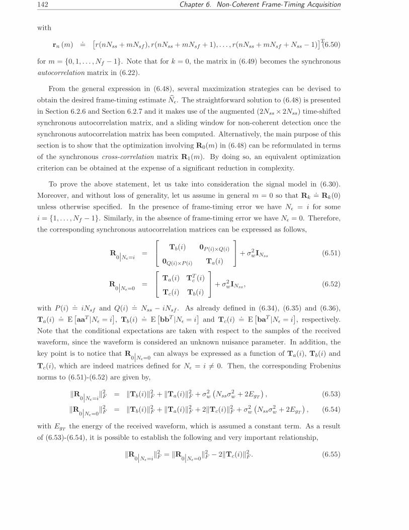
142 Chapter 6. Non-Coherent Frame-Timing Acquisition
with
rn (m).=
[r(nNss + mNsf ), r(nNss + mNsf + 1), . . . , r(nNss + mNsf + Nss − 1)
]T(6.50)
for m = {0, 1, . . . , Nf − 1}. Note that for k = 0, the matrix in (6.49) becomes the synchronous
autocorrelation matrix in (6.22).
From the general expression in (6.48), several maximization strategies can be devised to
obtain the desired frame-timing estimate Nǫ. The straightforward solution to (6.48) is presented
in Section 6.2.6 and Section 6.2.7 and it makes use of the augmented (2Nss × 2Nss) time-shifted
synchronous autocorrelation matrix, and a sliding window for non-coherent detection once the
synchronous autocorrelation matrix has been computed. Alternatively, the main purpose of this
section is to show that the optimization involving R0(m) in (6.48) can be reformulated in terms
of the synchronous cross-correlation matrix R1(m). By doing so, an equivalent optimization
criterion can be obtained at the expense of a significant reduction in complexity.
To prove the above statement, let us take into consideration the signal model in (6.30).
Moreover, and without loss of generality, let us assume in general m = 0 so that Rk.= Rk(0)
unless otherwise specified. In the presence of frame-timing error we have Nǫ = i for some
i = {1, . . . , Nf − 1}. Similarly, in the absence of frame-timing error we have Nǫ = 0. Therefore,
the corresponding synchronous autocorrelation matrices can be expressed as follows,
R0∣∣Nǫ=i
=
Tb(i) 0P (i)×Q(i)
0Q(i)×P (i) Ta(i)
+ σ2
wINss (6.51)
R0∣∣Nǫ=0
=
Ta(i) TT
c (i)
Tc(i) Tb(i)
+ σ2
wINss , (6.52)
with P (i).= iNsf and Q(i)
.= Nss − iNsf . As already defined in (6.34), (6.35) and (6.36),
Ta(i).= E
[aaT |Nǫ = i
], Tb(i)
.= E
[bbT |Nǫ = i
]and Tc(i)
.= E
[baT |Nǫ = i
], respectively.
Note that the conditional expectations are taken with respect to the samples of the received
waveform, since the waveform is considered an unknown nuisance parameter. In addition, the
key point is to notice that R0∣∣Nǫ=0
can always be expressed as a function of Ta(i), Tb(i) and
Tc(i), which are indeed matrices defined for Nǫ = i 6= 0. Then, the corresponding Frobenius
norms to (6.51)-(6.52) are given by,
‖R0∣∣Nǫ=i
‖2F = ‖Tb(i)‖2
F + ‖Ta(i)‖2F + σ2
w
(Nssσ
2w + 2EgT
), (6.53)
‖R0∣∣Nǫ=0
‖2F = ‖Tb(i)‖2
F + ‖Ta(i)‖2F + 2‖Tc(i)‖2
F + σ2w
(Nssσ
2w + 2EgT
), (6.54)
with EgTthe energy of the received waveform, which is assumed a constant term. As a result
of (6.53)-(6.54), it is possible to establish the following and very important relationship,
‖R0∣∣Nǫ=i
‖2F = ‖R
0∣∣Nǫ=0
‖2F − 2‖Tc(i)‖2
F . (6.55)

6.3. Frame-Timing Acquisition via the Multifamily Likelihood Ratio Test 143
The first important point is to notice that ‖R0∣∣Nǫ=0
‖2F is by definition, a constant term which
depends on the energy of the received waveform but not on the frame-timing error. This is
because R0∣∣Nǫ=0
assumes by definition no frame-timing error. Therefore, the information re-
garding the frame-timing error must be contained within the matrix Tc(i), according to (6.55).
The second important point is to notice that the structure of the synchronous cross-correlation
matrix is,
R1∣∣Nǫ=i
=
0P (i)×P (i) 0P (i)×Q(i)
Tc(i) 0Q(i)×Q(i)
. (6.56)
That is, the synchronous cross-correlation matrix of the received signal is based on the matrix
Tc(i), which indeed contains the information regarding the frame-timing error. Thus, R1 is
a sufficient statistic for the recovery of the frame-timing error. In fact, the dimensions of the
unknown but non-zero matrix Tc(i) are Q(i) × P (i), so they are directly related to the frame-
timing error Nǫ = i. Consequently, the optimization criterion in (6.48) can be recast as,
Nǫ = arg max0≤m≤Nf−1
‖R0(m)‖2F ≡ arg min
0≤m≤Nf−1‖R1(m)‖2
F . (6.57)
Based on (6.57), the synchronous cross-correlation matrix R1 allows an alternative strategy
for the frame-timing error acquisition. The advantage of this approach is that it makes use of
the (Nss × Nss) matrix R1 instead of the augmented (2Nss × 2Nss) matrix R0 used in Section
6.2.6. As a result, the computational burden is significantly reduced, especially by taking into
consideration that the number of samples per symbol may be a very large number when dealing
with UWB signals.
However, it should be pointed out that it is not straightforward to determine the dimensions
of the matrix Tc(i) from R1. Since the matrix Tc(i) exists only when Nǫ = i 6= 0, the detection
of the case in which Nǫ = 0 should be done by evaluating a signal detection threshold. When
the threshold is exceeded, the dimensions of Tc(i) would be determined to get the frame-timing
error. When the threshold is not exceeded, then the frame-timing error would be directly set
to Nǫ = 0. This strategy is very unpleasant, since it involves a two-step procedure and the
signal detection threshold depends on the working point of the scenario under consideration.
In order to circumvent this limitation, a simpler approach is proposed next by considering the
synchronous overlapped cross-correlation matrix.
6.3.2 Synchronous overlapped cross-correlation matrix for the frame-timing
acquisition problem
The synchronous overlapped cross-correlation (SOCC) matrix is a particular case of the gener-
alized cross-correlation matrix in (6.49) and it is defined as,
Rk (m, l).= E
[rn (m) rT
n+k (m + l)]
(6.58)
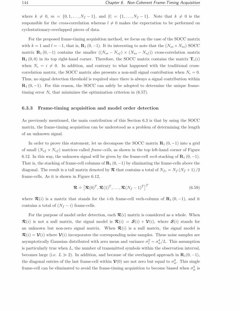
144 Chapter 6. Non-Coherent Frame-Timing Acquisition
where k 6= 0, m = {0, 1, . . . , Nf − 1}, and |l| = {1, . . . , Nf − 1}. Note that k 6= 0 is the
responsible for the cross-correlation whereas l 6= 0 makes the expectation to be performed on
cyclostationary-overlapped pieces of data.
For the proposed frame-timing acquisition method, we focus on the case of the SOCC matrix
with k = 1 and l = −1, that is, R1 (0,−1). It its interesting to note that the (Nss ×Nss) SOCC
matrix R1 (0,−1) contains the smaller ((Nss − Nsf ) × (Nss − Nsf )) cross-correlation matrix
R1 (0, 0) in its top right-hand corner. Therefore, the SOCC matrix contains the matrix Tc(i)
when Nǫ = i 6= 0. In addition, and contrary to what happened with the traditional cross-
correlation matrix, the SOCC matrix also presents a non-null signal contribution when Nǫ = 0.
Thus, no signal detection threshold is required since there is always a signal contribution within
R1 (0,−1). For this reason, the SOCC can safely be adopted to determine the unique frame-
timing error Nǫ that minimizes the optimization criterion in (6.57).
6.3.3 Frame-timing acquisition and model order detection
As previously mentioned, the main contribution of this Section 6.3 is that by using the SOCC
matrix, the frame-timing acquisition can be understood as a problem of determining the length
of an unknown signal.
In order to prove this statement, let us decompose the SOCC matrix R1 (0,−1) into a grid
of small (Nsf ×Nsf ) matrices called frame-cells, as shown in the top left-hand corner of Figure
6.12. In this way, the unknown signal will be given by the frame-cell vech stacking of R1 (0,−1).
That is, the stacking of frame-cell columns of R1 (0,−1) by eliminating the frame-cells above the
diagonal. The result is a tall matrix denoted by R that contains a total of Nfc = Nf (Nf + 1) /2
frame-cells. As it is shown in Figure 6.12,
R.=
[R(0)T , R(1)T , . . . ,R(Nf − 1)T
]T(6.59)
where R(i) is a matrix that stands for the i-th frame-cell vech-column of R1 (0,−1), and it
contains a total of (Nf − i) frame-cells.
For the purpose of model order detection, each R(i) matrix is considered as a whole. When
R(i) is not a null matrix, the signal model is R(i) = S(i) + V(i), where S(i) stands for
an unknown but non-zero signal matrix. When R(i) is a null matrix, the signal model is
R(i) = V(i) where V(i) incorporates the corresponding noise samples. These noise samples are
asymptotically Gaussian distributed with zero mean and variance σ2v = σ4
w/L. This assumption
is particularly true when L, the number of transmitted symbols within the observation interval,
becomes large (i.e. L ≫ 2). In addition, and because of the overlapped approach in R1(0,−1),
the diagonal entries of the last frame-cell within V(0) are not zero but equal to σ2w. This single
frame-cell can be eliminated to avoid the frame-timing acquisition to become biased when σ2w is
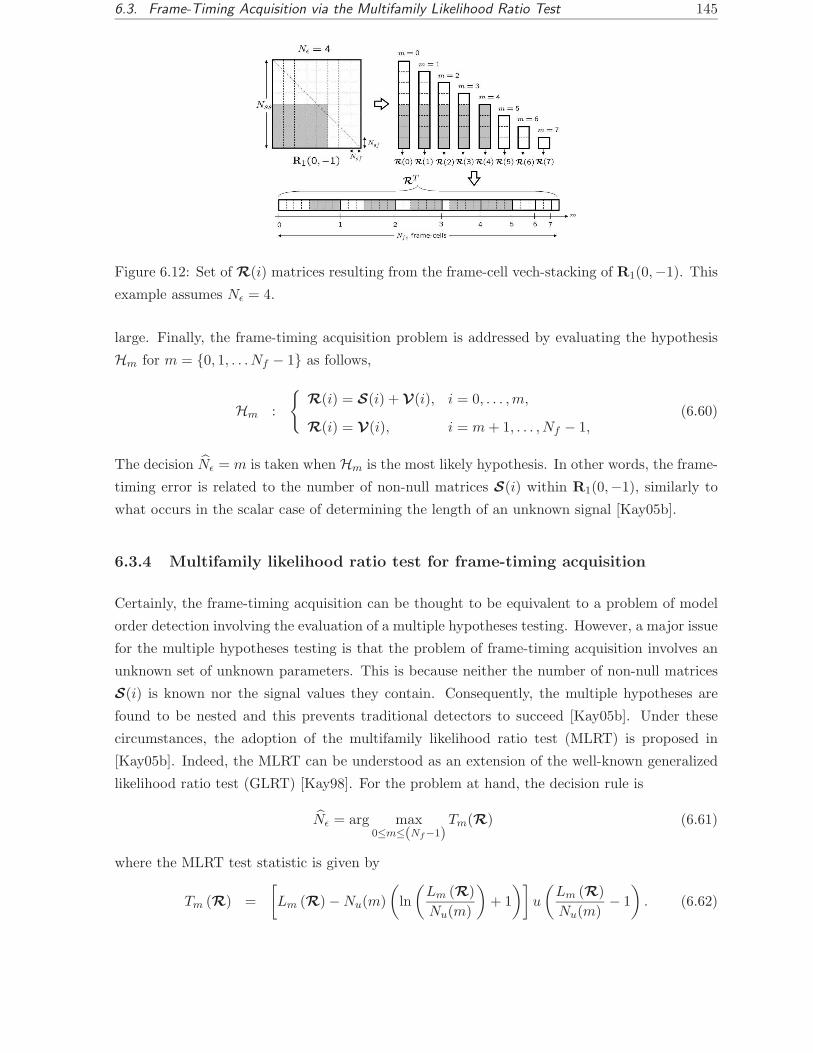
6.3. Frame-Timing Acquisition via the Multifamily Likelihood Ratio Test 145
Figure 6.12: Set of R(i) matrices resulting from the frame-cell vech-stacking of R1(0,−1). This
example assumes Nǫ = 4.
large. Finally, the frame-timing acquisition problem is addressed by evaluating the hypothesis
Hm for m = {0, 1, . . . Nf − 1} as follows,
Hm :
{R(i) = S(i) + V(i), i = 0, . . . , m,
R(i) = V(i), i = m + 1, . . . , Nf − 1,(6.60)
The decision Nǫ = m is taken when Hm is the most likely hypothesis. In other words, the frame-
timing error is related to the number of non-null matrices S(i) within R1(0,−1), similarly to
what occurs in the scalar case of determining the length of an unknown signal [Kay05b].
6.3.4 Multifamily likelihood ratio test for frame-timing acquisition
Certainly, the frame-timing acquisition can be thought to be equivalent to a problem of model
order detection involving the evaluation of a multiple hypotheses testing. However, a major issue
for the multiple hypotheses testing is that the problem of frame-timing acquisition involves an
unknown set of unknown parameters. This is because neither the number of non-null matrices
S(i) is known nor the signal values they contain. Consequently, the multiple hypotheses are
found to be nested and this prevents traditional detectors to succeed [Kay05b]. Under these
circumstances, the adoption of the multifamily likelihood ratio test (MLRT) is proposed in
[Kay05b]. Indeed, the MLRT can be understood as an extension of the well-known generalized
likelihood ratio test (GLRT) [Kay98]. For the problem at hand, the decision rule is
Nǫ = arg max0≤m≤(Nf−1)
Tm(R) (6.61)
where the MLRT test statistic is given by
Tm (R) =
[Lm (R) − Nu(m)
(ln
(Lm (R)
Nu(m)
)+ 1
)]u
(Lm (R)
Nu(m)− 1
). (6.62)

146 Chapter 6. Non-Coherent Frame-Timing Acquisition
1) Calculate an estimate for the SOCC matrix R1(0,−1) as,
R1(0,−1) = 1L
∑L−1n=0 rn(0)rn+1(−1)
with rn (m).=
[r(nNss + mNsf ), r(nNss + mNsf + 1), . . . , r(nNss + mNsf + Nss − 1)
]T.
2) for m = 0 : (Nf − 1),
• Evaluate the GLRT for the problem at hand,
Lm (R) = 1σ2
v
∑m
n=0 ‖R(n)‖2F
• Calculate the total number of samples (unknowns) considered in Lm (R)
Nu(m) = (m + 1)(Nf − m
2
)
• Evaluate the MLRT test statistic Tm (R) according to (6.62).
Tm (R) =
[Lm (R) − Nu(m)
(ln
(Lm(R)Nu(m)
)+ 1
)]u
(Lm(R)Nu(m) − 1
).
end
4) Decide Nǫ=arg maxm Tm (R)
Table 6.2: Procedure for the proposed frame-timing acquisition method based on the multifamily
likelihood ratio test (MLRT).
In (6.62), the term Nu(m) stands for the total number of unknowns when Hm is evaluated,
whereas u(x) denotes the unit step function. It is important to note that Lm (R) is the GLRT
under the hypothesis Hm, that is, by assuming that Nǫ = m. Therefore, the MLRT first
computes the GLRT for each hypothesis and then it applies a nonlinear transformation that
penalizes the GLRT as the model order increases. As a consequence, the MLRT provides a
better performance than the simple GLRT and is able to implement a detector/estimator scheme
in the presence of nested signal models. For a more detailed and comprehensive presentation of
the MLRT, the reader is referred to [Kay05b] and [Kay05a].
From the above considerations, the procedure in Table 6.2 is proposed to determine the
frame-timing error by evaluating the MLRT test statistic.
6.3.5 Simulation results
Computer simulations have been carried out to validate the performance of the proposed frame-
timing acquisition method. The results are compared with the dirty template (DT) technique
in [Yan04a] and the low-SNR unconditional maximum likelihood (lowSNR-UML) technique in
Section 6.2.6 - 6.2.7. The simulated scenario considers the transmission of ultra-short pulses
corresponding to the second derivative of the Gaussian pulse with a total duration of 4ns. The
UWB channel is randomly generated according to the channel model CM1 proposed by Intel
[Foe03] whose maximum delay spread is set to be in the order of 78ns. To test the robustness
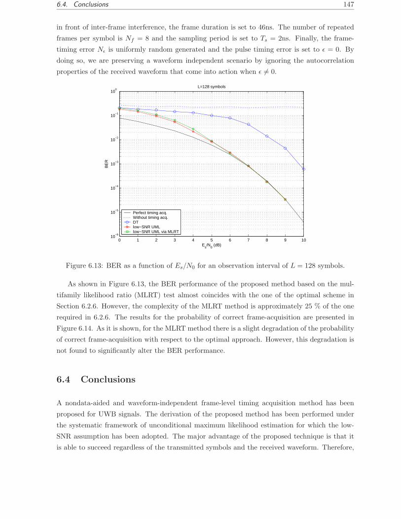
6.4. Conclusions 147
in front of inter-frame interference, the frame duration is set to 46ns. The number of repeated
frames per symbol is Nf = 8 and the sampling period is set to Ts = 2ns. Finally, the frame-
timing error Nǫ is uniformly random generated and the pulse timing error is set to ǫ = 0. By
doing so, we are preserving a waveform independent scenario by ignoring the autocorrelation
properties of the received waveform that come into action when ǫ 6= 0.
0 1 2 3 4 5 6 7 8 9 1010
−6
10−5
10−4
10−3
10−2
10−1
100
Es/N
0 (dB)
BE
R
L=128 symbols
Perfect timing acq.Without timing acq.DTlow−SNR UMLlow−SNR UML via MLRT
Figure 6.13: BER as a function of Es/N0 for an observation interval of L = 128 symbols.
As shown in Figure 6.13, the BER performance of the proposed method based on the mul-
tifamily likelihood ratio (MLRT) test almost coincides with the one of the optimal scheme in
Section 6.2.6. However, the complexity of the MLRT method is approximately 25 % of the one
required in 6.2.6. The results for the probability of correct frame-acquisition are presented in
Figure 6.14. As it is shown, for the MLRT method there is a slight degradation of the probability
of correct frame-acquisition with respect to the optimal approach. However, this degradation is
not found to significantly alter the BER performance.
6.4 Conclusions
A nondata-aided and waveform-independent frame-level timing acquisition method has been
proposed for UWB signals. The derivation of the proposed method has been performed under
the systematic framework of unconditional maximum likelihood estimation for which the low-
SNR assumption has been adopted. The major advantage of the proposed technique is that it
is able to succeed regardless of the transmitted symbols and the received waveform. Therefore,
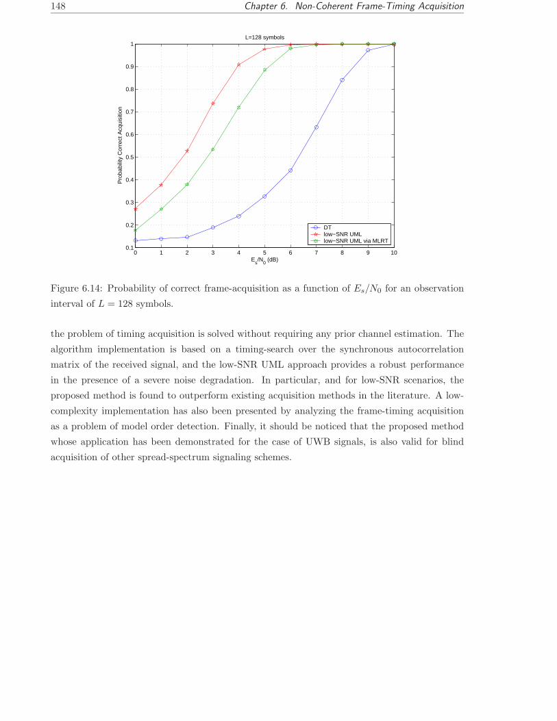
148 Chapter 6. Non-Coherent Frame-Timing Acquisition
0 1 2 3 4 5 6 7 8 9 100.1
0.2
0.3
0.4
0.5
0.6
0.7
0.8
0.9
1
Es/N
0 (dB)
Pro
babi
lity
Cor
rect
Acq
uisi
tion
L=128 symbols
DTlow−SNR UMLlow−SNR UML via MLRT
Figure 6.14: Probability of correct frame-acquisition as a function of Es/N0 for an observation
interval of L = 128 symbols.
the problem of timing acquisition is solved without requiring any prior channel estimation. The
algorithm implementation is based on a timing-search over the synchronous autocorrelation
matrix of the received signal, and the low-SNR UML approach provides a robust performance
in the presence of a severe noise degradation. In particular, and for low-SNR scenarios, the
proposed method is found to outperform existing acquisition methods in the literature. A low-
complexity implementation has also been presented by analyzing the frame-timing acquisition
as a problem of model order detection. Finally, it should be noticed that the proposed method
whose application has been demonstrated for the case of UWB signals, is also valid for blind
acquisition of other spread-spectrum signaling schemes.

6.A Derivation of the First Order Moment of χ (r; τ ; t;x) with Respect to x 149
Appendix 6.A Derivation of the First Order Moment of χ (r; τ ; t;x)
with Respect to x
This appendix is devoted to the derivation of Ex [χ (r; τ ; t;x)] as required in (6.15). For this
purpose, and from the definition of χ (r; τ ; t;x) in (6.13) we have,
Ex [χ (r; τ ; t;x)] =P−1∑
p=0
Ex
[xT
p
]AT
p r − 1
2
P−1∑
p=0
P−1∑
q=0
Ex
[xT
p ATp Aqxq
](6.63)
= −1
2
P−1∑
p=0
P−1∑
q=0
Tr(AT
p AqEx
[xqx
Tp
])(6.64)
= − 1
2P
P−1∑
p=0
Tr(AT
p Ap
)(6.65)
= − 1
2P
P−1∑
p=0
K∑
n=−K
aTn,pan,p (6.66)
= −L
2Et
.= γa (t) . (6.67)
As indicated in Section 6.2.1, the fact that Ex [xp] = 0 for any p, and Ex
[xpx
Tq
]= 1
P Iδpq, has
been used in (6.64) and (6.65) respectively. Moreover, it is important to note that the first order
moment of χ (r; τ ; t;x) with respect to x does not depend on the timing error τ but just on the
energy of the template waveform Et.= ‖an,p‖2 = ‖t‖2, which is a constant term.
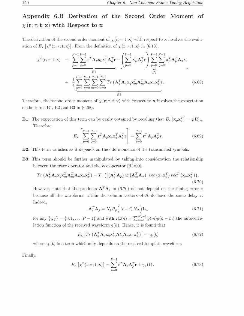
150 Chapter 6. Non-Coherent Frame-Timing Acquisition
Appendix 6.B Derivation of the Second Order Moment of
χ (r; τ ; t;x) with Respect to x
The derivation of the second order moment of χ (r; τ ; t;x) with respect to x involves the evalu-
ation of Ex
[χ2 (r; τ ; t;x)
]. From the definition of χ (r; τ ; t;x) in (6.13),
χ2 (r; τ ; t;x) =P−1∑
p=0
P−1∑
q=0
rTApxpxTq AT
q r
︸ ︷︷ ︸B1
−
P−1∑
p=0
xTp AT
p r
P−1∑
p=0
P−1∑
q=0
xTp AT
p Aqxq
︸ ︷︷ ︸B2
+1
4
P−1∑
p=0
P−1∑
q=0
P−1∑
m=0
P−1∑
n=0
Tr(AT
p AqxqxTmAT
mAnxnxTp
)
︸ ︷︷ ︸B3
. (6.68)
Therefore, the second order moment of χ (r; τ ; t;x) with respect to x involves the expectation
of the terms B1, B2 and B3 in (6.68).
B1: The expectation of this term can be easily obtained by recalling that Ex
[xpx
Tq
]= 1
P Iδpq.
Therefore,
Ex
P−1∑
p=0
P−1∑
q=0
rTApxpxTq AT
q r
=
P−1∑
p=0
rTApATp r. (6.69)
B2: This term vanishes as it depends on the odd moments of the transmitted symbols.
B3: This term should be further manipulated by taking into consideration the relationship
between the trace operator and the vec operator [Har00],
Tr(AT
p AqxqxTmAT
mAnxnxTp
)= Tr
([(AT
q Ap
)⊗
(AT
mAn
)]vec
(xnx
Tp
)vecT
(xmxT
q
)).
(6.70)
However, note that the products ATi Aj in (6.70) do not depend on the timing error τ
because all the waveforms within the column vectors of A do have the same delay τ .
Indeed,
ATi Aj = NfRg
((i − j) N∆
)IL, (6.71)
for any {i, j} = {0, 1, . . . , P − 1} and with Rg(n) =∑Ng−1
m=0 g(m)g(n − m) the autocorre-
lation function of the received waveform g(k). Hence, it is found that
Ex
[Tr
(AT
p AqxqxTmAT
mAnxnxTp
)]= γb (t) (6.72)
where γb (t) is a term which only depends on the received template waveform.
Finally,
Ex
[χ2 (r; τ ; t;x)
]=
P−1∑
p=0
rTApATp r + γb (t) . (6.73)
Chapter 7
Conclusions and Future Work
This thesis has analyzed the problem of coherent and non-coherent communication based on
ultra-wideband signaling. Because of the very large bandwidth occupancy of UWB signals,
the topic addressed in this dissertation has been placed within the framework of communication
under the wideband regime. However, and under a given fixed power constraint, wideband regime
has been shown to be equivalent to low-SNR working conditions. Thus, both wideband regime
and low-SNR have become the key elements in our analysis of digital ultra-wideband receivers.
This can be shown in Figure 7.1, where wideband regime and low-SNR are the starting points of
the subsequent discussions. The topics where contributions have been presented are highlighted
in this figure for the sake of clarity.
Let us first consider the topic of communication under the wideband regime. This topic has
been shown to result in the distinction between coherent and non-coherent receivers depending
on whether channel state information is available or not. This is an important issue because,
unlike traditional narrowband communication systems, the severe propagation conditions of
UWB signals involve a high complexity at the receiver side when coherent reception is adopted.
In this way, the goal of Chapter 3 has been to determine the performance bounds for both
coherent and non-coherent receivers so that the expected performance loss incurred by non-
coherent receivers can be evaluated. This has constituted the first part of this dissertation.
Once the theoretical analysis of coherent and non-coherent receivers has been addressed, the
next step has been to move forward into the receiver design. This has constituted the second
part of this dissertation. The basic tasks to be considered at the receiver are signal synchroniza-
tion, symbol detection and channel estimation (when required). For the case of coherent UWB
receivers, Chapter 4 has shown that the major problem is related with waveform estimation.
However, once the received waveform is identified, both synchronization and symbol detection
can be done in a standard manner as for traditional narrowband receivers. For this reason only
waveform estimation has been addressed when referring to the receiver design for coherent com-
151

152 Chapter 7. Conclusions and Future Work
munications. For the case of non-coherent UWB receivers, second-order cyclostationarity has
been shown to be essential to compensate the lack of knowledge about the received waveform.
With the aid of second-order statistics, Chapter 5 and Chapter 6 have dealt with the symbol
detection strategy and synchronization techniques, respectively.
Figure 7.1: Schematic overview of the topics covered within the present dissertation.
Next, we summarize the contributions and future research lines for each of the topics ad-
dressed in this dissertation.
Coherent vs. Non-Coherent Communications
The discussion on coherent versus non-coherent receivers is addressed in Chapter 3 under an
information theoretic approach. The main goal has been to characterize in an analytical manner
the asymptotic behavior when operating under the wideband regime. To this end, the notion of
constellation-constrained capacity provides an insightful measure on the achievable data rates
for an arbitrarily small error probability. Contrary to the traditional measure of capacity,
constellation-constrained capacity has been adopted to model the fact that we are dealing with
digital communication systems. That is, to model the fact that we are dealing with discrete
input distributions.
In the recent literature, most of the results dealing with achievable data rates for UWB

153
systems are based on numerical evaluations to overcome the difficulty in providing a closed-form
expression for capacity. In this part of the dissertation, however, one of the most important
contributions is that closed-form expressions are provided to upper-bound the constellation-
constrained capacity for both coherent and non-coherent UWB systems. The proposed closed-
form upper bounds have been compared with the exact (i.e. numerically evaluated) results and
a tight match has been found.
In a second step, the analysis of the results for constellation-constrained capacity of UWB
systems has led to an important conclusion. There exists the traditional belief that capacity
in the AWGN channel can also be achieved in the presence of unknown fading provided that
bandwidth is sufficiently large. This statement led to the assumption that UWB systems (i.e.
very large bandwidth signaling) would achieve the same capacity as in the AWGN channel when
propagating in the presence of unknown multipath fading channels. This was expected to be a
very attractive result since it suggests that channel estimation would not be necessary for UWB
systems. However, one of the most important results from the theory of spectral efficiency
in the wideband regime is that capacity for the AWGN cannot be achieved in the presence
of unknown fading when bandwidth is very large but finite, and when peakiness constraints
are introduced. Peakiness constraints become necessary because UWB systems must co-exist
with existing wireless communication systems and thus, harmful interference must be avoided.
However, peakiness constraints come at the expense of a degradation loss in the achievable data
rates of non-coherent receivers when compared to coherent receivers.
When operating under the wideband regime, capacity results shown in Figure 3.8 suggest a
performance degradation from 9 to 10 dB. This degradation is experienced in terms of Eb/N0
when non-coherent UWB reception is implemented instead of coherent UWB reception. How-
ever, high data rates can still be provided due to the very large bandwidth of UWB signals.
This has been shown in Figure 3.9, where the achievable data rates for non-coherent UWB sys-
tems are also found to be more sensitive to changes in Eb/N0 than the achievable data rates for
coherent UWB systems.
Some of the topics that have not been addressed in this dissertation but may be subject to
further investigation are the following:
• It would be interesting to extend the capacity analysis presented herein to the case where
cognitive radio is implemented. Cognitive radio is an attractive paradigm for UWB com-
munications since it allows to dynamically adapt the transmission and radiation param-
eters so as to exploit available spectral resources without interfering licensed users1. In
that way, it is possible to exceed the allowable radiation limits of standard UWB systems
by shaping the spectrum so as to incorporate inactive frequency bands. That is, by using
1The interested reader may found an excellent presentation on cognitive radio in [Hay05].

154 Chapter 7. Conclusions and Future Work
frequency bands of licensed users when these users are not inactive. The analysis of this
new approach would involve the assumption of colored noise in our signal model. With
some prior information about the licensed services that are supposed to be operated in
a specific time and geographical location, the noise spectral mask of the received data
provides information on active and not active users and services. This information can be
represented in terms of a given noise correlation matrix whose impact in terms of capacity
should be evaluated.
• A pending issue to be further analyzed is the relationship between capacity and likelihood
ratio testing according to Eq. (3.23). This is an important issue since the meaning of
Eq. (3.23) suggests that a clear link may be established between information theory and
detection theory.
• Closed-form expressions have been provided for upper-bounding the constellation-
constrained capacity of both coherent and non-coherent UWB communications. However,
it would be interesting to further analyze the behavior of these upper-bounds in the limit of
infinite bandwidth and to compare the results with the exact infinite-bandwidth capacity
of Gaussian inputs in Eq. (3.9).
• Since tight upper-bounds have been derived for constellation-constrained capacity, tight
lower-bounds are also required to restrict the region where capacity may range.
• In a context of random time variations of the propagation channel, and because of the
particular signaling structure of UWB communication systems, it is reasonable to consider
the transmission of random waveforms from a given waveform distribution. In that case,
it is important to determine the optimal waveform distribution to maximize capacity
for a given characterization of the propagation channel. Note that this approach is in
contrast with the traditional implementation of UWB systems, where a deterministic pulse
is usually transmitted.
• Possible extensions of the work presented herein includes the adoption of multiple-input
multiple-output schemes and the impact of multi-user interference.
Waveform Estimation for Coherent Receivers
Coherent receivers assume perfect knowledge of the propagation conditions between transmitter
and receiver. As indicated in Figure 7.1, coherent receivers require side information in the
form of waveform or channel state information in order to proceed with their basic tasks (e.g.
synchronization and symbol detection). The provision of channel state information has been
shown to be a critical and computationally demanding problem in UWB receivers due to the
severe and unique distortion of the UWB propagation channel.

155
In this dissertation, the waveform estimation problem has been approached from the low-
SNR perspective. In this sense, the second-order statistics of the received signal have been
shown to become the sufficient statistics for the problem at hand. As already indicated in the
pioneering work by Tong et al., channel estimation is possible from second-order statistics when
more than one sample per symbol is considered. Following this approach, the proposed waveform
estimation technique is aimed at exploiting the cyclostationary properties of the second-order
statistics of the received UWB signal. This has been shown to be possible by considering the
synchronous autocorrelation matrix of the received signal, and by properly defining a precise
signal model to represent the finite-length structure of the UWB received signal. Based on the
above considerations, a waveform estimation technique has been derived in Chapter 4 which
differs in many aspects with traditional approaches. Some of the most important features of the
proposed method are listed below:
1. The aggregated channel response and not the individual paths and amplitudes is pro-
posed to be estimated. This constitutes an unstructured approach where the paths of the
propagation channel are completely disregarded and the received waveform for a single
transmitted pulse is considered as a whole.
2. The unconditional maximum likelihood criterion is considered. As a result, the uncon-
ditional approach leads to a nondata-aided implementation of the waveform estimation
technique whereas the maximum likelihood perspective allows an asymptotically unbiased
and efficient performance.
3. The low-SNR approximation of the unconditional maximum likelihood criterion is adopted.
Therefore, the resulting estimator is especially designed to cope with the low-SNR condi-
tions of actual UWB receivers.
4. The likelihood criterion is compressed with information regarding the signal subspace.
This restricts the solution space around the true value in order to avoid any possible ill-
conditioning or local-maxima. This subspace-compressed approach can be understood as
a principal component analysis, and thus, a significant reduction in the computational
burden is obtained through a tradeoff between bias and variance.
5. The proposed solution can be understood as a correlation matching method. That is, it
performs a matching between the synchronous autocorrelation of the received signal and
the synchronous autocorrelation of the signal model. Indeed, correlation matching methods
have been previously proposed in the literature for nondata-aided channel estimation, but
the problem has been found to be nonlinear and the solution is usually obtained in a rather
heuristic manner by numerical evaluation or gradient-based search.
6. Contrary to most of the traditional approaches, a closed-form expression for the proposed
waveform estimator is provided. This is done by converting the nonlinear optimization
156 Chapter 7. Conclusions and Future Work
problem into a linear least-squares problem on the second-order statistics of the received
signal.
Simulation results have been obtained for the proposed waveform estimation technique and
a superior performance is observed when compared to existing methods based on second-order
statistics. However, there are still some pending issues to be further investigated,
• Some research is still required to determine the identifiability conditions for the proposed
closed-form waveform estimation technique. This issue was already discussed in Section
4.4.1 and the main problem was to find a formal proof to guarantee the full column rank
condition of matrix Q in (4.24). This matrix can be thought to be the system matrix in
a traditional least squares problem and thus, its full column rank condition is essential to
guarantee the uniqueness of the solution.
• Extensive simulation results should also be obtained with different channel models within
the IEEE 802.15.3a/4 standards. This would provide a more robust characterization of
the proposed waveform estimation technique under different working conditions.
• Since a wide range of channel estimation methods have already been proposed in the liter-
ature, it is interesting to perform a more exhaustive comparison to assess the performance
of the proposed technique.
• Finally, another pending issue is the one related with the extension of the current formu-
lation to accommodate multi-user scenarios.
Symbol Detection for Non-Coherent Receivers
It has been shown that the adoption of coherent receivers (i.e the assumption of perfect channel
state information) is restricted to those applications where slow channel variations are experi-
enced and significant computational complexity is available at the receiver. This is due to the
fact that the large multipath resolution of UWB signals makes the computation of fast and
accurate channel estimates a challenging and computationally demanding task. When such a
computational burden is not available, there is no choice but to resort to non-coherent receivers.
Non-coherent receivers have been previously addressed in the literature. However, most of
the times an unknown deterministic approach is considered by assuming the received waveform
to be unknown but constant during all the observation interval. Alternatively, other approaches
consider the problem of waveform time-variation by adopting transmitted reference (TR) signal-
ing, which is based on the transmission of a reference pulse prior to each data modulated pulse.
In that way, noisy channel state information is provided by the received unmodulated pulses
157
themselves. However, this comes at the expense of an efficiency loss due to the transmission of
unmodulated pulses and at the end, a coherent receiver is required once again.
Contrary to previous contributions, the problem of symbol detection for non-coherent re-
ceivers has been addressed in this dissertation by assuming the received signal to be random.
The low-SNR maximum likelihood criterion has also been adopted for deriving the optimal
framework for the symbol detection problem of binary-PPM. Two different analyses for this
problem have been presented depending on whether the amplitudes of the received waveforms
are correlated or not. For uncorrelated scenarios, the optimal symbol detector has been shown to
be based on the exploitation of the power delay profile of the channel. For correlated scenarios,
the optimal symbol detector has been found to result in a rather intricate expression. In that
case, however, significant simplifications can be introduced by allowing the implementation of a
rank-1 receiver. This low cost alternative can be implemented by adopting an information theo-
retic criterion for deciding the optimal deterministic linear receiver to be selected among the set
of signal subspace eigenvectors. In particular, this criterion has been shown to be based on the
minimization of the system bit error rate through the maximization of the Jeffreys’ divergence
between the two symbol hypotheses to be decided.
Some of the topics that have not been addressed in this dissertation but may be subject to
further investigation are the following:
• As already mentioned in Chapter 5, the proposed symbol detection techniques are based
on the assumption that the received signal is Gaussian distributed. This allows the symbol
detection problem to be mathematically tractable but, fortunately, it also corresponds to
some realistic scenarios such as the one encountered in the propagation of UWB signals
in industrial environments [Sch05b], [Sch05c]. For other scenarios such as office or resi-
dential environments, the statistics of UWB received signals cannot be properly modeled
as Gaussian. Instead, Nakagami or log-normal distributions are found to provide a closer
match. Consequently, it would be interesting to evaluate the performance of the proposed
detectors in those scenarios where the received statistics are not Gaussian.
• A practical issue to be considered is the one related with reducing the complexity of the
proposed detectors. As shown in Chapter 5, a relatively high computational burden is
required to obtain the optimal symbol decision statistics. This is especially true for the
case of correlated scattering scenarios where a simple rank one approach was suggested
to alleviate the required complexity. However, suboptimal approaches to the problem of
symbol detection in non-coherent receivers should be investigated.
• Again, and similarly to the waveform estimation problem, another pending issue is the one
related with the extension of the current formulation to accommodate multi-user scenarios.

158 Chapter 7. Conclusions and Future Work
Synchronization for Non-Coherent Receivers
In the absence of any prior knowledge about the propagation conditions, the synchronization
problem for non-coherent receivers has been addressed through the exploitation of the cyclosta-
tionary properties of the received signal. The formal procedure is similar to the one adopted for
the non-coherent detection of UWB signals in the sense that the proposed method is based on
the analysis of the synchronous autocorrelation of the received signal. Moreover, since carrierless
UWB is considered along the present dissertation, synchronization reduces to timing acquisition.
As indicated in Chapter 6, synchronization of UWB receivers is similar to what happens
in traditional spread-spectrum communication systems. That is, timing acquisition is divided
into two different stages. First, coarse timing acquisition (i.e. frame-timing acquisition) and
second, fine timing acquisition (i.e. pulse-timing acquisition). The second stage has not been
considered for the case of non-coherent receivers because the notion of fine timing error is always
related to a reference pulse. Since no channel information is available in non-coherent receivers,
the reference waveform is unknown and thus fine timing error becomes part of the unknown
waveform.
There are two main contributions to be highlighted in the topic of timing synchronization of
UWB signals.
1. The problem of frame-timing acquisition has been formulated in a rigorous and analytical
manner by using the low-SNR approximation of the unconditional maximum likelihood
criterion. This is in contrast with many of the existing contributions on this topic, where
most of the techniques are obtained in a rather ad-hoc or heuristic manner. The major ad-
vantage of the proposed technique is that it is able to succeed regardless of the transmitted
symbols and the received waveform. Therefore, the problem of frame-timing acquisition
can be solved in the absence of pilot symbols and without requiring any prior channel
estimation. Finally, it has been shown that the optimal formulation of the problem leads
to a simple strategy where frame-timing error is obtained as a result of an energy detection
search over the synchronous autocorrelation matrix of the received signal.
2. A reduced complexity implementation has been proposed based on the principle of mul-
tifamily likelihood ratio testing. By doing so, the synchronization problem can be under-
stood as a model order detection problem. Compared to the optimal approach, the major
advantage of this low-cost solution is that at least 75 % of the computational complexity
can be saved at no cost in terms of performance.
In both cases, the performance results of the proposed frame-timing acquisition techniques
outperform existing contributions in the literature. However, some of the research lines that
still remain open are the following:
159
• The proposed frame-timing acquisition methods are based on the assumption that the
transmitted symbols are amplitude modulated. It would be interesting to extend the
results to the case where no amplitude modulation but only pulse position modulation is
being transmitted.
• Similarly to the symbol detection problem, low complexity receivers are strongly required
for UWB systems. For this reason, one of the pending issues in this part of the dissertation
is the investigation of suboptimal techniques that involve low-complexity and provide rapid
acquisition.


Bibliography
[Aie03] G. R. Aiello, G. D. Rogerson, “Ultra-Wideband Wireless Systems”, IEEE Microwave,Vol. 4, no 2, pags. 36–47, June 2003.
[And05] C. R. Anderson, A. Annamalai et al., Introduction to Ultra Wideband Communica-tion Systems, Prentice Hall Communications Engineering and Emerging TechnologiesSeries, Prentice Hall, 2005.
[Ara03] F. E. Aranda, N. Brown, H. Arslan, “RAKE Receiver Finger Assignment for Ultra-Wideband Radio”, Proc. 4th IEEE Workshop on Signal Processing Advances in Wire-less Communications (SPAWC), pags. 239–243, 15-18 June 2003.
[Bar00] T. W. Barrett, “History of UltraWideband (UWB) Radar & Communications: Pio-neers and Innovators”, Proc. Progress in Electromagnetics Symposium, 2000.
[Bel94] J. S. Belrose, “The Sounds of a Spark Transmitter: Telegraphy andTelephony”, Radioscientist , 22 December 1994, available online at:http://www.physics.otago.ac.nz/ursi/belrose/spark.html.
[Ben78] C. L. Benett, G. F. Ross, “Time-Domain Electromagnetics and Its Application”, Pro-ceedings of the IEEE , Vol. 66, pags. 299–318, 1978.
[Ben06] M. Di Benedetto, T. Kaiser, A. F. Molisch, I. Oppermann, C. Politano, D. Porcino(eds.), UWB Communication Systems. A Comprehensive Overview , EURASIP BookSeries on Signal Processing and Communications, Hindawi Publising Corporation,2006.
[Ber02] I. Bergel, E. Fishler, H. Messer, “Narrow-band Interference Suppression in Time-Hopping Impulse-Radio Systems”, Proc. IEEE Conference on Ultra Wideband Systemsand Technologies, pags. 303–308, 2002.
[Bla03] R. Blazquez, P. Newaskar, A. Chandrakasan, “Coarse Acquisition for Ultra WidebandDigital Receivers”, Proc. IEEE International Conference on Acoustics, Speech andSignal Processing (ICASSP), Vol. 4, pags. 137–140, 6-10 April 2003.
[Bla87] R. E. Blahut, Principles and Practice of Information Theory , Addison-Wesley, 1987.
[Brz06] G. Brzezina, L. Roy, L. MacEachern, “Planar Antennas in LTCC Technology withTransceiver Integration Capability for Ultra-Wideband Applications”, IEEE Trans.Microwave Theory Tech., Vol. 54, no 6, pags. 2830–2839, June 2006, part 2.
[Bue04] R. M. Buehrer, W. A. Davis, A. Safaai-Jazi, D. Sweeney, “Ultra-WidebandPropagation Measurements and Modeling - Final Report to DARPA NETEX
i

ii Bibliography
Program”, Tech. rep., Virginia Tech. Antenna Group, 2004, Available at:http://www.mprg.org/people/buehrer/ultra/darpa%5Fnetex.shtml.
[Car01] M. Cardoza, et al., Final Report Data Collection Campaign for Measuring UWB/GPSCompatibility Effects, Center for Ultra-Wideband Research and Engineering, Univer-sity of Austin Texas, TL-SG-01-01, 26 February 2001.
[Car03] C. Carbonelli, U. Mengali, U. Mitra, “Synchronization and Channel Estimation forUWB Signals”, Proc. IEEE Global Conference on Communications (GLOBECOM),Vol. 2, pags. 764–768, 1-5 December 2003.
[Car04a] C. Carbonelli, S. Franz, U. Mengali, U. Mitra, “Semi-Blind ML Synchronization forUWB Transmitted Reference Systems”, Conference Record of the Thirty-Eigth Asilo-mar Conference on Signals, Systems and Computers, Vol. 2, pags. 1491–1495, 7-10November 2004.
[Car04b] C. Carbonelli, U. Mitra, “Clustered Channel Estimation for UWB Signals”, Proc.International Conference on Communications (ICC), Vol. 4, pags. 2432–2436, 20-24June 2004.
[Car06a] C. Carbonelli, U. Mengali, “M-PPM Noncoherent Receivers for UWB Applications”,IEEE Trans. Wireless Commun., Vol. 5, no 8, pags. 2285 – 2294, August 2006.
[Car06b] C. Carbonelli, U. Mengali, “Synchronization Algorithms for UWB Signals”, IEEETrans. Commun., Vol. 54, no 2, pags. 329–338, February 2006.
[Cas02a] D. Cassioli, M. Z. Win, A. F. Molisch, “The Ultra-Wide Bandwidth Indoor Channel:From Statistical Model to Simulations”, IEEE J. Select. Areas Commun., Vol. 20,no 6, pags. 1247–1257, August 2002.
[Cas02b] D. Cassioli, M. Z. Win, F. Vatalaro, A. F. Molisch, “Performance of Low-ComplexityRAKE Reception in a Realistic UWB channel”, Proc. IEEE International Conferenceon Communications, Vol. 2, pags. 763–767, 28 April - 2 May 2002.
[CEP06] ECC Decision of 24 March 2006 on the harmonised conditions for devices us-ing Ultra-Wideband (UWB) technology iin bands below 10.6 GHz , 24 March 2006,eCC/DEC/(06)04.
[Cha03] Y. Chao, R. A. Scholtz, “Optimal and Suboptimal Receivers for Ultra-WidebandTransmitted Reference Systems”, IEEE Global Conference on Communications(GLOBECOM), Vol. 2, pags. 759–763, 1-5 December 2003.
[Cha05] Y.-L. Chao, R. A. Scholtz, “Ultra-wideband transmitted reference systems”, IEEETrans. Veh. Commun., Vol. 54, no 5, pags. 1556–1569, September 2005.
[Che05] P. Cheong, A. Rabbachin, J.-P. Montillet, K. Yu, I. Opperman, “Synchronization,TOA and Position Estimation for Low-Complexity LDR UWB Devices”, IEEE Inter-national Conference on Ultra-Wideband , pags. 480–484, 2005.
[Chu04] X. Chu, R. D. Murch, “The Effect of NBI on UWB Time-Hopping Systems”, IEEETrans. Wireless Commun., Vol. 3, no 5, pags. 1431–1436, September 2004.
Bibliography iii
[Chu05] W. C. Chung, N. J. August, D. S. Ha, “Signaling and Multiple Access Techniquesfor Ultra Wideband 4G Wireless Communication Systems”, IEEE Wireless Commun.Mag., Vol. 12, no 2, pags. 46–55, April 2005.
[Con06] M. Converse, E. J. Bond, B. D. Veen, S. C. Hagness, “A Computational Studyof Ultra-Wideband versus Narrowband Microwave Hyperthermia for Breast CancerTreatment”, IEEE Trans. Microwave Theory Tech., Vol. 54, no 5, pags. 2169–2180,May 2006.
[Cov91] T. M. Cover, J. A. Thomas, Elements of Information Theory , John Wiley & Sons,1991.
[Cra98a] R. J.-M. Cramer, M. Z. Win, R. A. Scholtz, “Evaluation of the Multipath Charac-teristics of the Impulse Radio Channel”, Proc. 9th IEEE International Symposium onPersonal, Indoor and Mobile Radio Communications, Vol. 2, pags. 864–868, 8 - 11September 1998.
[Cra98b] R. J.-M. Cramer, M. Z. Win, R. A. Scholtz, “Impulse Radio Multipath Characteristicsand Diversity Reception”, Proc. IEEE International Conference on Communications(ICC), Vol. 3, pags. 1650–1654, 7-11 June 1998.
[Cra02] R. J.-M. Cramer, R. A.Scholtz, M. Z. Win, “Evaluation of an Ultra-Wide-Band Prop-agation Channel”, IEEE Trans. Antennas Propagat., Vol. 50, pags. 561–570, May2002.
[D’A05] A. A. D’Amico, U. Mengali, “GLRT Receivers for UWB Systems”, IEEE Commun.Lett., Vol. 9, no 6, pags. 487–489, June 2005.
[DAR90] Assessment of Ultra-Wideband (UWB) Technology , 13 July 1990, OSD/DARPA Ultra-Wideband Radar Review Panel, Battelle Tactical Technology Center, Contract No.DAAH01-88-C-0131, ARPA Order 6049.
[Dav79] J. R. Davis, D. J. Baker, J. P. Shelton, W. S. Ament, “Some Physical Constraints onthe Use of ”Carrier-Free” Waveforms in Radio-Wave Transmission Systems”, Proc.IEEE , Vol. 67, no 6, pags. 884–890, June 1979.
[Dju98] P. Djuric, “Asymptotic MAP Criteria for Model Selection”, IEEE Trans. Signal Pro-cessing , Vol. 46, pags. 2726–2735, October 1998.
[Dol00] S. Dolinar, D. Divsalar, J. Hamkins, F. Pollara, “Capacity of Pulse-Position Modula-tion (PPM) on Gaussian and Webb Channels”, Tech. rep., Jet Propulsion Laboratory(JPL), National Aeronautics and Space Administration (NASA), 2000, LPL TMOProgress Report.
[ECC05] The Protection Requirements of Radiocommunications Systems Below 10.6 GHz fromGeneric UWB Applications, February 2005, Electronics Communication Committee(ECC), CEPT, Report 64.
[Ett77] P. Van Etten, “The Present Technology of Impulse Radars”, Proc. International RadarConference, pags. 535–539, October 1977.
[FCC02] First Report and Order, Revision of Part 15 of the Commission’s Rules RegardingUltra-Wideband Transmission Systems, April 2002, FCC, Washington, DC. ET Docket98-153, FCC 02-48.

iv Bibliography
[Fen03] L. Feng, W. Namgoong, “Joint Estimation and Detection of UWB Signals with TimingOffset Error and Unknown Channel”, Proc. IEEE Conference on Ultra WidebandSystems and Technologies, pags. 152–156, 16-19 November 2003.
[Foe03] J. Foerster, Channel Modeling Sub-Committee Report (Final), IEEE P802.15 WorkingGroup for Wireless Personal Area Networks (WPANs), February 2003.
[For06] A. Fort, J. Ryckaert, C. Desset, P. De Doncker, P. Wambacq, L. Van Biesen, “Ultra-Wideband Channel Model for Communications Around the Human Body”, IEEE J.Select. Areas Commun., Vol. 24, no 4, pags. 927–933, April 2006.
[Fra03] S. Franz, U. Mitra, “On Optimal Data Detection for UWB Transmitted ReferenceSystems”, Proceedings IEEE Global Conference on Communications (GLOBECOM),Vol. 2, pags. 744–748, 1-5 December 2003.
[Gal68] R. G. Gallager, Information Theory and Reliable Communication, John Wiley andSons, New York, NY, 1968.
[Gar80] F. M. Gardner, “Self-Noise in Synchronizers”, IEEE Trans. Commun., Vol. 28,pags. 1159–1163, August 1980.
[Gar88] F. M. Gardner, Demodulator Reference Recovery Techniques Suited for Digital Im-plementation, Final Report: ESTEC Contract No. 6847/86/NL/DG, European SpaceAgency, 1988.
[Gee06] D. Geer, “UWB Standardization Efforts Ends in Controversy”, IEEE Computer ,Vol. 39, no 7, pags. 13–16, July 2006.
[Gez02] S. Gezici, E. Fishler, H. Kobayashi, H. V. Poor, A. F. Molisch, “A Rapid AcquisitionTechnique for Impulse Radio”, Proc. Pacific Communications, Computers and SignalProcessing , Vol. 2, pags. 627–630, 28-30 August 2002.
[Gez04] S. Gezici, H. Kobayashi, H. V. Poor, A. F. Molisch, “Optimal and Suboptimal LinearReceivers for Time-Hopping Impulse Radio Systems”, Proc. International Workshopon Ultra Wideband Systems (IWUWBS) Joint with Conference on Ultra WidebandSystems and Technologies (UWBST), pags. 11–15, 18-21 May 2004.
[Gez05] S. Gezici, Z. Tian, G. B. Giannakis, H. Kobayashi, A. F. Molisch, H. V. Poor,Z. Sahinoglu, “Localization via Ultra-Wideband Radios: A Look at Positioning As-pects for Future Sensor Networks”, IEEE Signal Processing Mag., Vol. 22, no 4,pags. 70–84, July 2005.
[Gha04] M. Ghavami, L. B. Michael, R. Kohno, Ultra Wideband Signals and Systems in Com-munication Engineering , John Wiley & Sons, 2004.
[Gia97] G. B. Giannakis, S. D. Halford, “Asymptotically Optimal Blind Fractionally SpacedChannel Estimation and Performance Analysis”, IEEE Trans. Signal Processing ,Vol. 45, pags. 1815–1830, July 1997.
[Git92] R. D. Gitlin, J. F. Hayes, S. B. Weinstein, Data Communications Principles, PlenumPress, 1992.
[Gol49] M. J. Golay, “Note on the Theoretical Efficiency of Information Reception with PPM”,Proceedings of the IRE , Vol. 37, pags. 1031, 1949.
Bibliography v
[Gol96] G. H. Golub, C. F. Van Loan, Matrix Computations, Johns Hopkins University Press,1996.
[Gue05] E. Gueguen, F. Thudor, P. Chambelin, “A Low Cost UWB Printed Dipole Antennawith High Performance”, Proc. IEEE International Conference on Ultra-Wideband ,pags. 89–92, 5-8 September 2005.
[Gur05a] M. C. Gursoy, H. V. Poor, S. Verdu, “The Noncoherent Rician Fading Channel. Part I:Structure of the Capacity-Achieving Input”, IEEE Trans. Wireless Commun., Vol. 4,no 5, pags. 2193–2206, September 2005.
[Gur05b] M. C. Gursoy, H. V. Poor, S. Verdu, “The Noncoherent Rician Fading Channel. PartII: Spectral Efficiency in the Low-Power Regime”, IEEE Trans. Wireless Commun.,Vol. 4, no 5, pags. 2207–2221, September 2005.
[Ham04] J. Hamkins, B. Moision, “Selection of Modulation and Codes for Deep Space Opti-cal Communications”, Proc. of SPIE, Free-Space Laser Communication TechnologiesXIV , Vol. 5338, pags. 123–130, 2004.
[Har68] H. F: Harmuth, “A generalized concept of frequency and some applications”, IEEETrans. Inform. Theory , Vol. 14, no 3, pags. 375–381, May 1968.
[Har69a] H. F. Harmuth, “Applications of Walsh Functions in Communications”, IEEE Spectr.,pags. 82–91, November 1969.
[Har69b] H. F. Harmuth, Transmission of Information by Orthogonal Functions, Springer Ver-lag, 1969.
[Har79] H. F. Harmuth, “Comments on ”Some Physical Constraints on the Use of ”Carrier-Free” Waveforms in Radio-Wave Transmission Systems””, Proc. IEEE , Vol. 67, no 6,pags. 890–891, June 1979.
[Har00] D. A. Harville, Matrix Algebra from a Statistician’s Perspective, Springer, 2000.
[Har04] R. Harjani, J. Harvey, R. Sainati, “Analog/RF Physical Layer Issues for UWB Sys-tems”, Proc. 17th International Conference on VLSI Design, pags. 941–948, 2004.
[Hay05] S. Haykin, “Cognitive Radio: Brain-Empowered Wireless Communications”, IEEE J.Select. Areas Commun., Vol. 23, no 2, pags. 201–220, February 2005.
[Hoc02] R. T. Hoctor, H. W. Tomlinson, An Overview of Delay-Hopped, Transmitted-ReferenceRF Communications, January 2002, G. E. Research and Development Center, Tech-nical Information Series, pp. 1-29.
[Hoe61] C. H. Hoeppner, Pulse Communication System, 5 September 1961, U.S. Patent2.999.128.
[Hom02] E. A. Homier, R. A. Scholtz, “Rapid Acquisition of Ultra-Wideband Signals in theDense Multipath Channel”, Proc. IEEE Conf. on Ultra Wideband Systems and Tech-nologies, pags. 105–109, 21-23 May 2002.
[hop01] “Final Report, UWB-GPS Compatibility Analysis Project”, 8 March 2001, John Hop-kins University, Applied Physics Laboratory.

vi Bibliography
[Hoy03] S. Hoyos, B. M. Sadler, G. R. Arce, “Dithering and Sigma-Delta Modulation in Mono-bit Digital Receivers for Ultra-Wideband Communications”, Proc. IEEE Conf. onUltra Wideband Systems and Technologies, pags. 71–75, 16-19 November 2003.
[Hoy04] S. Hoyos, B. Sadler, G. R. Arce, “High-Speed A/D Conversion for Ultra-WidebandSignals Based on Signal Projection over Basis Functions”, Proc. IEEE InternationalConference on Acoustics, Speech and Signal Processing (ICASSP), Vol. 4, pags. 537–540, 17-21 May 2004.
[Hoy05] S. Hoyos, B. Sadler, G. R. Arce, “Monobit Digital Receivers for Ultrawideband Com-munications”, IEEE Trans. Wireless Commun., Vol. 4, no 4, pags. 1337–1344, July2005.
[Hua96a] Y. Hua, “Fast Maximum Likelihood for Blind Identification of Multiple FIR Chan-nels”, IEEE Trans. Signal Processing , Vol. 44, no 3, pags. 661–672, March 1996.
[Hua96b] Y. Hua, M. Waz, “Strict Identifiability of Multiple FIR Channels Driven by an Un-known Arbitrary Sequence”, IEEE Trans. Signal Processing , Vol. 44, no 3, pags. 756–759, March 1996.
[Hua02] Y. Huang, J. Benesty, “Adaptive Blind Channel Identification: Multi-Channel LeastMean Square and Newton Algorithms”, Proc. International Conference on Acoustics,Speech and Signal Processing (ICASSP), Vol. 2, pags. 1637–1640, 2002.
[Int04] Intel, Ultra-Wideband (UWB Technology). Enabling High-Speed Wire-less Personal Area Networks, Intel Corporation, 2004, Available at:http://www.intel.com/technology/ultrawideband/downloads/Ultra-Wideband.pdf.
[Int05a] Intel, Ultra-Wideband (UWB Technology). One Step Closerto Wireless Freedom, Intel Corporation, 2005, Available at:http://www.intel.com/technology/comms/uwb/download/wireless%5Fpb.pdf.
[Int05b] Intel, Wireless USB. The First High-Speed Personal Wire-less Interconnect , Intel Corporation, 2005, Available at:http://www.intel.com/technology/comms/wusb/download/wirelessUSB.pdf.
[Jac63] I. Jacobs, “The Asymptotic Behavior of Incoherent M-ary Communication Systems”,Proceedings of the IRE , Vol. 51, no 1, pags. 251–252, 1963.
[Jef46] H. Jeffreys, “An Invariant Form for the Prior Probability in Estimation Problems”,Proc. Roy. Soc. Lon., A, pags. 453–461, 1946.
[Kar04] J. Karedal, S. Wyne, P. Almers, F. Tufvesson, A. F. Molisch, “Statistical Analysis ofthe UWB Channel in an Industrial Environment”, Proc. IEEE Vehicular TechnologyConference (VTC-Fall), pags. 81–85, 2004.
[Kay93] S. M. Kay, Fundamentals of Statistical Signal Processing. Estimation Theory , Vol. I,Prentice Hall, 1993.
[Kay98] S. M. Kay, Fundamentals of Statistical Signal Processing. Detection Theory , Vol. II,Prentice Hall, 1998.

Bibliography vii
[Kay05a] S. M. Kay, “Exponentially Embedded Families-New Approaches to Model Order Es-timation”, IEEE Trans. Aerosp. Electron. Syst., Vol. 41, no 1, pags. 333–345, January2005.
[Kay05b] S. M. Kay, “The Multifamily Likelihood Ratio Test for Multiple Signal Model Detec-tion”, IEEE Signal Processing Lett., Vol. 12, no 5, pags. 369–371, May 2005.
[Ken69] R. S. Kennedy, Fading Dispersive Communication Channels, John Wiley and Sons,New York, NY, 1969.
[Kol04] R. Kolic, “Ultra Wideband - The Next-Generation Wireless Connection”, Tech-nology @ Intel Magazine, pags. 1–6, February/March 2004, Available at:http://www.intel.com/technology/magazine/communications/wi02042.pdf.
[Kon05] W. Kong, Y. Zhu, G. Wang, “Effects of Pulse Distortion in UWB Radiation on UWBImpulse Communications”, Proc. International Conference on Wireless Communica-tions, Networking and Mobile Computing (WCNM), Vol. 1, pags. 344–347, Sept. 23-262005.
[Kul97] S. Kullback, Information Theory and Statistics, Dover Publications, 1997.
[Lam10] H. Lamb, “The Diffraction of a Solitary Wave”, Proceedings of the London Mathemat-ical Society , Vol. 2, no 8, pags. 422–437, 1910.
[Le05] B. Le, T. W. Rondeau, J. H. Reed, C. W. Bostian, “Analog-to-Digital Converters”,IEEE Signal Processing Mag., Vol. 22, no 6, pags. 69–77, November 2005.
[Lee04] J.-Y. Lee, S. Choi, “Through-Material Propagation Characteristic and Time Reso-lution of UWB Signal”, Proc. International Workshop on Ultra Wideband Systems(IWUWBS) Joint with Conference on Ultra Wideband Systems and Technologies(UWBST), pags. 71–75, 18-21 May 2004.
[Li00] Y. Li, X. Huang, “The Spectral Evaluation and Comparison for Ultra-Wideband Sig-nals with Different Modulation Schemes”, Proc. World Multiconf. on Systemics, Cy-bernetics and Informatics (SCI), pags. 277–282, July 2000.
[Li05] X. Li, E. J. Bond, B. D. Veen, C. S. Hagness, “An overview of ultra-wideband mi-crowave imaging via space-time beamforming for early-stage breast-cancer detection”,IEEE Antennas Propagat. Mag., Vol. 47, no 1, pags. 19–34, February 2005.
[Liu94] H. Liu, G. Xu, L. Tong, “A Deterministic Approach to Blind Identification of Mul-tichannel FIR Systems”, Proc. IEEE International Conference on Acoustics, Speechand Signal Processing (ICASSP), Vol. IV, pags. 581–584, 19-22 April 1994.
[Liu96] H. Liu, G. Xu, L. Tong, T. Kailath, “Recent Developments in Blind Channel Equal-ization: From Cyclostationarity to Subspaces”, Signal Processing, Elsevier , Vol. 50,pags. 83–99, 1996.
[Lot00] V. Lottici, A. D’Andrea, U. Mengali, “Channel estimation for ultra-wideband commu-nications”, IEEE J. Select. Areas Commun., Vol. 20, no 9, pags. 1638–1645, December2000.

viii Bibliography
[Lou00] P. Loubaton, E. Moulines, P. Regalia, Signal Processing Advances in Wireles andMobile Communications, Vol. 1, Prentice-Hall, 2000, Chapter 3: Subspace Methodfor Blind Identification and Deconvolution.
[Lov02] W. M. Lovelace, J. K. Townsend, “The Effects of Timing Jitter and Tracking onthe Performance of Impulse Radio”, IEEE J. Select. Areas Commun., Vol. 20, no 9,pags. 1646–1651, December 2002.
[Low05] Z. N. Low, J. H. Cheong, C. L. Law, “Low-Cost PCB Antenna for UWB Applications”,IEEE Antennas Wireless Propagat. Lett., Vol. 4, pags. 237–239, 2005.
[LS04] J. A. Lopez-Salcedo, G. Vazquez, “Frequency Domain Iterative Pulse Shape Estima-tion Based on Second Order Statistics”, Proc. 5th IEEE Workshop on Signal Process-ing Advances in Wireless Communications (SPAWC), Lisbon, Portugal, 11-14 July2004.
[Luo00] M. Luo, D. Akos, S. Pullen, P. Enge, Potential Interference to GPS from UWB Trans-mitters, Test Results. Phase 1A: Accuracy and Loss-of-Lock Testing for Aviation Re-ceivers, Stanford University, 26 October 2000.
[Luo02] C. Luo, M. Medard, “Frequency-Shift Keying for Ultrawideband. Achieving Rates onthe Order of Capacity”, Proc. 40th Annual Allerton Conference on Communication,Control and Computing , Monticello, Illinois (USA), October 2002.
[Luo05] X. Luo, G. B. Giannakis, “Blind Timing Acquisition for Ultra-Wideband Multi-UserAd-Hoc Access”, Proc. IEEE International Conference on Acoustics, Speech and Sig-nal Processing (ICASSP), Vol. III, pags. 313–316, 18-23 March 2005.
[Mar00] C. J. Le Martret, G. B. Giannakis, “All-Digital PAM Impulse Radio for Multiple-Access Through Frequency-Selective Multipath”, IEEE Global Conference on Com-munications (GLOBECOM), Vol. 1, pags. 77–81, 27 Nov. - 1 Dec. 2000.
[Mas76] J. L. Massey, “All Signal Sets Centered About the Origin are Optimal at Low Energy-to-Noise Ratios on the AWGN Channel”, Proc. IEEE International Symposium onInformation Theory (ISIT), pags. 80–81, June 1976.
[Men97] U. Mengali, A. N. D’Andrea, Synchronization Techniques for Digital Receivers,Plenum Press, 1997.
[Men05] A. Menouni, R. Knopp, R. Saadane, “Subspace Analysis of Indoor UWB Channels”,EURASIP Journal on Applied Signal Processing , Vol. 3, pags. 287–295, 2005.
[Mie03] B. Mielczarek, M. O. Wessman, A. Svensson, “Performance of Coherent UWB RAKEReceivers with Channel Estimators”, Proc. IEEE Vehicular Technology ConferenceFall , Vol. 3, pags. 1880–1884, 6-9 October 2003.
[Mir01] F. Ramirez Mireles, “On the Performance of Ultra-Wide-Band Signals in GaussianNoise and Dense Multipath”, IEEE Trans. Veh. Technol., Vol. 50, no 1, pags. 244–249, January 2001.
[Mof76] D. L. Moffatt, R. J. Puskar, “A Subsurface Electromagnetic Pulse Radar”, Geophysics,, no 41, pags. 506–518, 1976.
Bibliography ix
[Mol04] A. F. Molisch, IEEE 802.15.4a Channel Model Final Report , IEEE P802.15 WorkingGroup for Wireless Personal Area Networks (WPANs), November 2004.
[Mol05] A. F. Molisch, “Ultrawideband Propagation Channels-Theory, Measurement and Mod-eling”, IEEE Trans. Veh. Technol., Vol. 54, no 5, pags. 1528–1545, September 2005.
[Mor74] R. N. Moray, Geophysical Survey System Employing Electromagnetic Pulses, April1974, U.S. Patent 3.806.795.
[Mou95] E. Moulines, P. Duhamel, J.-F. Cardoso, S. Mayrargue, “Subspace Methods for theBlind Identification of Multichannel FIR Filters”, IEEE Trans. Signal Processing ,Vol. 43, no 2, pags. 516–525, February 1995.
[Nak03] Y.-P. Nakache, A. F. Molisch, “Spectral Shape of UWB Signals - Influence of Modula-tion Format, Multiple Access Scheme and Pulse Shape”, Proc. 57th IEEE SemiannualConference on Vehicular Technology (VTC-Spring), Vol. 4, pags. 2510–2514, 22-25April 2003.
[Nam03] W. Namgoong, “A Channelized Digital Ultrawideband Receiver”, IEEE Trans. Wire-less Commun., Vol. 2, no 3, pags. 502–510, May 2003.
[Nos04] H. Nosaka, M. Nakamura, M. Ida, K. Kurishima, T. Shibata, M. Tokumitsu,M. Muraguchi, “A 24-Gsps 3-bit Nyquist ADC using InP HBTs for Electronic Disper-sion Compensation”, Proc. IEEE MTT-S International Microwave Symposium, Vol. 1,pags. 101–104, 6-11 June 2004.
[Oh05] M.-K. Oh, B. Jung, R. Harjani, D.J. Park, “A New Noncoherent UWB Impulse RadioReceiver”, IEEE Commun. Lett., Vol. 9, no 2, pags. 151–153, February 2005.
[Ott93] B. Ottersten, M. Viberg, P. Stoica, A. Nehorai, Radar Array Processing , Springer-Verlag, 1993, Chapter 4: Maximum Likelihood Techniques for Parameter Estimation.
[Par03] B. Parr, B. Cho, K. Wallace, Z. Ding, “A Novel Ultra-Wideband Pulse Design Algo-rithm”, IEEE Commun. Lett., Vol. 7, no 4, pags. 219–221, Mayy 2003.
[Pie66] J. R. Pierce, “Ultimate Performance of M-ary Transmissions on Fading Channels”,IEEE Trans. Inform. Theory , Vol. 12, no 1, pags. 2–5, 1966.
[Por05] D. Porrat, “Information Theory of Wideband Communications. A Tutorial”, 2005,http://www.cs.huji.ac.il/ dporrat/WidebandTutorial.pdf.
[Pri58] R. Price, P. E. Green, “A Communication Technique for Multipath Channels”, Pro-ceedings of the IRE , Vol. 46, pags. 555–570, March 1958.
[Pro94] J. G. Proakis, M. Salehi, Communication Systems Engineering , Prentice-Hall Inter-national Editions, 1994.
[Pro01] J. G. Proakis, Digital Communications, McGraw-Hill, 4th Edition, international edi-tion ed., 2001.
[Qiu95] R. C. Qiu, Time/Frequency Dispersion of Digital Transmission Media, PhD Thesis,Polytechnic University, Brooklyn, New York, 1995.

x Bibliography
[Qiu96] R. C. Qiu, “Wideband Wireless Multipath Channel Modeling with Path Frequency De-pendence”, Proc. IEEE International Conference on Communications (ICC), Vol. 1,pags. 277–281, Dallas, Texas, USA, 23-27 June 1996.
[Qiu02] R. C. Qiu, “A Study of the Ultra-Wideband Wireless Propagation Channel andOptimum UWB Receiver Design”, IEEE J. Select. Areas Commun., Vol. 20, no 9,pags. 1628–1637, December 2002.
[Qiu04] R. C. Qiu, “A Generalized Time Domain Multipath Channel and Optimal ReceiverDesign - Part II: Physics-Based System Analysis”, IEEE Trans. Wireless Commun.,Vol. 3, no 6, pags. 2312–2324, November 2004.
[Qiu05] R. C. Qiu, C. Zhou, Q. Liu, “Physics-Based Pulse Distortion for Ultra-WidebandSignals”, IEEE Trans. Veh. Technol., Vol. 54, no 5, pags. 1546–1555, September 2005.
[Rab04a] A. Rabbachin, I. Oppermann, “Synchronization Analysis for UWB Systems with aLow-Complexity Energy Collection Receiver”, 2004 International Workshop on UltraWideband Systems (IWUWBS) Joint with Conference on Ultra Wideband Systems andTechnologies (UWBST), pags. 288–292, Kyoto, Japan, May 2004.
[Rab04b] A. Rabbachin, L. Stoica, S. Tiuraniemi, I. Oppermann, “A Low Cost, Low PowerUWB Based Sensor Network”, Proc. International Workshop on Wireless Ad-HocNetworks, pags. 84–88, 31 May - 3 June 2004.
[Rao04] C. Rao, B. Hassibi, “Analysis of Multiple-Antenna Wireless Links at Low SNR”, IEEETrans. Inform. Theory , Vol. 50, no 9, pags. 2123–2130, September 2004.
[Reg05] L. Reggiani, G. M. Maggio, “Rapid Search Algorithms for Code Acquisition in UWBImpulse Radio Communications”, IEEE J. Select. Areas Commun., Vol. 23, no 5,pags. 898–908, May 2005.
[Ros54] L. A. De Rosa, Random Impulse System, 9 March 1954, U.S. Patent 2.671.896.
[Ros73] G. F. Ross, K. W. Robbins, Base-Band Radiation and Reception System, 12 June1973, U.S. Patent 3.739.392.
[Ros86] G. F. Ross, Early Developments and Motivations for Time-Domain Analysis and Ap-plications. Time-Domain Measurements in Electromagnetics, Van Nostrand Reinhold,1986.
[Rus64] C. K. Rushforth, “Transmitted-Reference Techniques for Random or Unknown Chan-nels”, IEEE Trans. Inform. Theory , Vol. 10, no 1, pags. 39–42, January 1964.
[Saa04] R. Saadane, A. Menouni, R. Knopp, D. Aboutajdine, “Empirical Eigenanalysis ofIndoor UWB Propagation Channels”, Proc. IEEE Global Conference on Communica-tions (GLOBECOM), pags. 3215–3219, December 2004.
[Sah05] M. E. Sahin, H. Arslan, “Narrowband Interference Identification Approach for UWBSystems”, Proc. IEEE Military Communications Conference (MILCOM), Vol. 3, pags.1404–1408, 17-20 October 2005.
[Sal87] A. Saleh, R. Valenzuela, “A Statistical Model for Indoor Multipath Propagation”,IEEE J. Select. Areas Commun., Vol. 5, no 2, pags. 128–137, February 1987.
Bibliography xi
[Sch93] R. A. Scholtz, “Multiple Access with Time-Hopping Impulse Modulation”, Proc. IEEEConference on Military Communications (MILCOM), Vol. 2, pags. 447–450, October1993.
[Sch05a] R. A. Scholtz, D. M. Pozar, W. Namgoong, “Ultra-Wideband Radio”, EURASIPJournal on Applied Signal Processing , Vol. 2005, no 3, pags. 252–272, 2005.
[Sch05b] U. G. Schuster, H. Bolcskei, “How Different are UWB Channels from ConventionalWideband Channels?”, Proc. International Workshop on Convergent Technologies,Oulu, Finland, June 2005.
[Sch05c] U. G. Schuster, H. Bolcskei, “Ultra-Wideband Channel Modeling on the Basis ofInformation-Theoretic Criteria”, Proc. International Symposium on Information The-ory (ISIT), pags. 97–101, 4-9 September 2005.
[Sch06] B. Schechner, Ultrawideband Shipments to Reach Nearly 300 Million in 2011Despite Apparent Barriers, ABI Research, 15 May 2006, Available at:http://www.abiresearch.com/abiprdisplay.jsp?pressid=648.
[Sha48] C. E. Shannon, “A Mathematical Theory of Communication”, Bell Syst. Tech. J.,Vol. 27, July-Oct. 1948.
[She03] H. Sheng, A. M. Haimovich, A. F. Molisch, J. Zhang, “Optimum Combining for TimeHopping Impulse Radio UWB RAKE Receivers”, Proc. IEEE Conference on UltraWideband Systems and Technologies, pags. 224–228, 16-19 November 2003.
[Slo94] D. Slock, “Blind Factionally-Spaced Equalization, Perfect Reconstruction, Filter-banks, and Multilinear Prediction”, Proc. IEEE International Conference on Acous-tics, Speech and Signal Processing (ICASSP), Vol. 4, pags. 585–588, April 1994.
[Som01] A. Sommerfield, “Theoretisches Uber die Beugung der Roentgenstrahlen”, Zeitschriftfur Mathematik und Physik , Vol. 46, pags. 11–97, 1901.
[Sou03] Y. Souilmi, R. Knopp, “On the Achievable Rates of Ultra-Wideband PPM with Non-Coherent Detection in Multipath Environments”, Proc. IEEE International Confer-ence on Communications (ICC), Vol. 5, pags. 3530–3534, Anchorage, Alaska, USA,11-15 May 2003.
[Sto04] L. Stoica, S. Tiuraniemi, H. Repo, A. Rabbachin, I. Oppermann, “Low Complex-ity UWB Circuit Transceiver Architecture for Low Cost Sensor Tag Systems”, Proc.IEEE International Symposium on Personal, Indoor and Mobile Radio Communica-tions (PIMRC), Vol. 1, pags. 196–200, 5-8 September 2004.
[Sun93] F. W. Sun, H. C. Van Tilborg, “Approaching Capacity by Equiprobable Signalingon the Gaussian Channel”, IEEE Trans. Inform. Theory , Vol. 39, pags. 1714–1716,September 1993.
[Tan05a] J. Tang, Z. Xu, “A Novel Modulation Diversity Assisted Ultra-Wideband Communi-cation System”, Proc. IEEE International Conference on Acoustics, Speech and SignalProcessing (ICASSP), Vol. 3, pags. 309–312, Philadelphia, USA, March 2005.
[Tan05b] J. Tang, Z. Xu, B. M. Sadler, “Digital Receiver for TR-UWB Systems with Inter-PulseInterference”, Proc. 6th IEEE Workshop on Signal Processing Advances in WirelessCommunications (SPAWC), pags. 420–424, 5-8 June 2005.

xii Bibliography
[Tay94] J. D. Taylor, Introduction to Ultra-Wideband Radar Systems, CRC Press, 1994.
[Tel00] I. E. Telatar, D. N. Tse, “Capacity and Mutual Information of Wideband MultipathFading Channels”, IEEE Trans. Inform. Theory , Vol. 46, no 4, pags. 1384–1400, 2000.
[Tia02] Z. Tian, L. Yang, G. B. Giannakis, “Symbol Timing Estimation in Ultra WidebandCommunications”, Proc. 36th Asilomar Conference on Signals, Systems and Comput-ers, Vol. 2, pags. 1924–1928, Pacific Grove, California, USA, 3-6 November 2002.
[Tia05a] Z. Tian, H. Ge, L. L. Scharf, “Low-Complexity Multiuser Detection and Reduced-Rank Wiener Filters for Ultra-Wideband Multiple Access”, Proc. IEEE InternationalConference on Acoustics, Speech and Signal Processing (ICASSP), Vol. 3, pags. 621–624, 18-23 March 2005.
[Tia05b] Z. Tian, G. B. Giannakis, “BER Sensitivity to Mistiming in Ultra-Wideband ImpulseRadios - Part I: Nonrandom Channels”, IEEE Trans. Signal Processing , Vol. 53, no 4,pags. 1550–1560, April 2005.
[Tia05c] Z. Tian, G. B. Giannakis, “BER Sensitivity to Mistiming in Ultra-Wideband ImpulseRadios - Part II: Fading Channels”, IEEE Trans. Signal Processing , Vol. 53, no 5,pags. 1897–1907, May 2005.
[Tia05d] Z. Tian, G. B. Giannakis, “A GLRT Approach to Data-Aided Timing Acquisition inUWB Radios - Part I: Algorithms”, IEEE Trans. Wireless Commun., Vol. 4, no 6,pags. 2956–2967, November 2005.
[Tia05e] Z. Tian, G. B. Giannakis, “A GLRT Approach to Data-Aided Timing Acquisition inUWB Radios - Part II: Training Sequence Design”, IEEE Trans. Wireless Commun.,Vol. 4, no 6, pags. 2994–3004, November 2005.
[Ton91] L. Tong, G. Xu, T. Kailath, “A New Approach to Blind Identification and Equalizationof Multipath Channels”, Proc. 25th Asilomar Conference on Signals, Systems andComputers, Vol. 2, pags. 856–860, Pacific Grove, California, USA, 4-6 November 1991.
[Ton94] L. Tong, G. Xu, T. Kailath, “Blind Identification and Equalization Based on Second-order Statistics: A Time Domain Approach”, IEEE Trans. Inform. Theory , Vol. 40,no 2, pags. 340–349, March 1994.
[Ton98] L. Tong, S. Perreau, “Multichannel Blind Identification: From Subspace Methods toMaximum Likelihood Methods”, Proc. IEEE , Vol. 86, no 10, pags. 1951–1968, October1998.
[Tre83] J. R. Treichler, B. G. Agee, “A New Approach to Multipath Correction of ConstantModulus Signals”, IEEE Trans. Acoust., Speech, Signal Processing , Vol. 31, pags. 459–472, April 1983.
[Tur59] G. L. Turin, “The Asymptotic Behavior of Ideal M-ary Systems”, Proceedings of theIRE , Vol. 47, pags. 93–94, 1959.
[Ung82] G. Ungerboeck, “Channel Coding with Multilevel/Phase Signals”, IEEE Trans. In-form. Theory , Vol. 28, no 1, pags. 55–67, January 1982.
[Van03] H. L. VanTrees, Detection, Estimation, and Modulation Theory , Vol. I, John Wileyand Sons, 2001-2003.

Bibliography xiii
[Vee05] A. J. van der Veen, A. Leshem, Robust Adaptive Beamforming , Wiley Interscience,2005, Chapter 6: Constant Modulus Beamforming.
[Ver02a] S. Verdu, “Recent Results on the Capacity of Wideband Channels in the Low-PowerRegime”, IEEE Wireless Commun. Mag., Vol. 9, no 4, pags. 40–45, August 2002.
[Ver02b] S. Verdu, “Spectral Efficiency in the Wideband Regime”, IEEE Trans. Inform. The-ory , Vol. 48, no 6, pags. 1319–1343, June 2002.
[Vil05] J. Villares, G. Vazquez, “Second-Order Parameter Estimation”, IEEE Trans. SignalProcessing , Vol. 53, pags. 2408–2420, July 2005.
[Vaz00] G. Vazquez, J. Riba, Signal Processing Advances in Wireless and Mobile Communi-cations, Vol. 2, Prentice-Hall, 2000, Chapter 9: Non-Data-Aided Digital Synchroniza-tion.
[Wal99] R. H. Walden, “Analog-to-digital converter survey and analysis”, IEEE J. Select.Areas Commun., Vol. 17, no 4, pags. 539–550, April 1999.
[Wan05] S. B.-T. Wang, Design of Ultra-Wideband RF Front-End , PhDThesis, University of California, Berkeley, 2005, Available at:http://bwrc.eecs.berkeley.edu/Publications/2005/THESES/S. Wang/S. BoTingWang Thesis.pdf.
[Wei04] M. Weisenhorn, W. Hirt, “Robust Noncoherent Receiver Exploiting UWB ChannelProperties”, Proc. International Workshop on Ultra Wideband Systems (IWUWBS)Joint with Conference on Ultra Wideband Systems and Technologies (UWBST), pags.156–160, Kyoto, Japan, May 2004 2004.
[Wei05] M. Weisenhorn, W. Hirt, “ML Receiver for Pulsed UWB Signals and Partial ChannelState Information”, Proc. IEEE International Conference on Ultra-Wideband , pags.180–185, 5-8 September 2005.
[Wil03] R. D. Wilson, R. A. Scholtz, “Template Estimation in Ultra-Wideband Radio”, Proc.37th Asilomar Conference on Signals, Systems and Computers, Vol. 2, pags. 1244–1248, 9-12 November 2003.
[Win97] M. Z. Win, R. A. Scholtz, “Energy Capture vs. Correlator Resources in Ultra-WideBandwidth Indoor Wireless Communications Systems”, Proc. IEEE Conference onMilitary Communications (MILCOM), Vol. 3, pags. 1277–1281, 2-5 November 1997.
[Win98] M. Z. Win, R. A. Scholtz, “Impulse Radio: How It Works”, IEEE Commun. Lett.,Vol. 2, no 2, pags. 36–38, February 1998.
[Win00] M. Z. Win, R. A. Scholtz, “Ultra-Wide Bandwidth Time-Hopping Spread-SpectrumImpulse Radio for Wireless Multiple-Access Communications”, IEEE Trans. Com-mun., Vol. 48, no 4, pags. 679–691, April 2000.
[Win02] M. Z. Win, “Spectral Density of Random UWB Signals”, IEEE Commun. Lett., Vol. 6,no 12, pags. 526–528, December 2002.
[Woo00] J. P. Woodard, “Comparative Study of Turbo Decoding Techniques: An Overview”,IEEE Trans. Veh. Commun., Vol. 49, no 6, pags. 2208–2233, November 2000.

xiv Bibliography
[Woz65] J. M. Wozencraft, I. M. Jacobs, Principles of Communications Engineering , WavelandPress, 1965.
[Wu04] X. Wu, Z. Tian, T. N. Davidson, G. B. Giannakis, “Orthogonal waveform design foruwb radios”, Proc. 5th IEEE Workshop on Signal Processing Advances in WirelessCommunications (SPAWC), pags. 150–154, 11-14 July 2004.
[Wu06] J.-Y. Wu, T.-S. Lee, “Periodic-Modulation-Based Blind Channel Identification forSingle-Carrier Block Transmission with Frequency-Domain Equalization”, IEEETrans. Signal Processing , Vol. 54, no 3, pags. 1114–1130, March 2006.
[Xu95] G. Xu, H. Liu, L. Tong, T. Kailath, “A Least-Squares Approach to the Blind Chan-nel Identification”, IEEE Trans. Signal Processing , Vol. 43, no 12, pags. 2982–2993,December 1995.
[Xu01] Z. Xu, “Asymptotically Near-Optimal Blind Estimation of Multipath CDMA Chan-nels”, IEEE Trans. Signal Processing , Vol. 49, no 9, pags. 2003–2017, September 2001.
[Xu03a] Z. Xu, “Blind Channel Estimation via Subspace Approximation”, Proc. 37th Asilo-mar Conference on Signals, Systems and Computers, Vol. 2, pags. 1653–1657, 9-12November 2003.
[Xu03b] Z. Xu, J. Tang, P. Liu, “Blind Channel Estimation for Multiple Access UWB Com-munications Based on Periodic Time Hopping and Pulse-Rate Modeling”, Proc. IEEETopical Conference on Wireless Communication Technology , pags. 453–454, 15-17 Oc-tober 2003.
[Yan03a] L. Yang, G. B. Giannakis, “Low-Complexity Training for Rapid Timing Acquisitionin Ultra Wideband Communications”, Proc. IEEE Global Conference on Communi-cations (GLOBECOM), Vol. 2, pags. 769–773, 1-5 December 2003.
[Yan03b] L. Yang, Z. Tian, G. B. Giannakis, “Non-Data Aided Timing Acquisition of Ultra-Wideband Transmissions Using Cyclostationarity”, Proc. International Conference onAcoustics, Speech and Signal Processing , Vol. 4, pags. 121–124, 6-10 April 2003.
[Yan04a] L. Yang, G. B. Giannakis, “Blind UWB Timing with a Dirty Template”, Proc.IEEE International Conference on Acoustics, Speech and Signal Processing (ICASSP),Vol. IV, pags. 509–512, Montreal (Canada), 17-21 May 2004.
[Yan04b] L. Yang, G. B. Giannakis, “Ultra-Wideband Communications: An Idea Whose TimeHas Come”, IEEE Signal Processing Mag., Vol. 21, no 6, pags. 26–54, November 2004.
[Yan04c] L. Yang, G. B. Giannakis, A. Swami, “Noncoherent Ultra-Wideband Radios”, Proc.IEEE Conference on Military Communications (MILCOM), Vol. 2, pags. 786–791,Monterey, California, USA, 31 October - 3 November 2004.
[Yan05] L. Yang, G. B. Giannakis, “Timing Ultra-Wideband Signals with Dirty Templates”,IEEE Trans. Commun., Vol. 53, no 11, pags. 1952–1963, November 2005.
[Yan06] L. Yang, A. Swami, “Noncoherent Demodulator for PPM-UWB Radios”, Proc.IEEE International Conference on Acoustics, Speech and Signal Processing (ICASSP),Vol. 4, pags. 501–504, 14-19 May 2006.
Bibliography xv
[Yao04] W. Yao, Y. Wang, “Direct Antenna Modulation - A Promise for Ultra-Wideband(UWB) Transmitting”, Proc. IEEE MTT-S International Microwave Symposium,Vol. 2, pags. 1273–1276, 6-11 June 2004.
[Yaz04] K. Y. Yazdandoost, R. Kohno, “Ultra Wideband Antenna”, IEEE Commun. Mag.,Vol. 42, no 6, pags. 29–32, June 2004.
[Yaz05] K. Y. Yazdandoost, R. Kohno, “Slot Antenna for Ultra Wideband System”, Proc.IEEE/ACES International Conference on Wireless Communications and AppliedComputational Electromagnetics, pags. 212–216, 3-7 April 2005.
[Yin04] Z. Ying, J. Andersson, “An Ultra Wideband ”Cobra” Patch Antenna”, IEE Pro-ceedings in Microwaves, Antennas and Propagation, Vol. 151, no 6, pags. 486–490,December 2004.
[Zar05] K. Zarifi, A. B. Gershman, “Enhanced Blind Subspace-Based Signature WaveformEstimation in CDMA Systems with Circular Noise”, Proc. IEEE International Con-ference on Acoustics, Speech and Signal Processing (ICASSP), Vol. 3, pags. 937–940,18-23 March 2005.
[Zen97a] H. H. Zeng, L. Tong, “Blind Channel Estimation Using the Second-Order Statistics:Asymptotic Performance and Limitations”, IEEE Trans. Signal Processing , Vol. 45,no 8, pags. 2060–2071, August 1997.
[Zen97b] H. H. Zeng, L. Tong, “Blind Channel Estimation Using the Second-Order Statistics:Algorithms”, IEEE Trans. Signal Processing , Vol. 45, no 8, pags. 1919–1930, August1997.
[Zha01] L. Zhao, A. M. Haimovich, “Capacity of M-ary PPM Ultra-Wideband Communica-tions over AWGN Channels”, Proc. IEEE Vehicular Technology Conference (VTC),Vol. 2, pags. 1191–1195, 2001.
[Zha03] J. Zhang, T. D. Abhayapala, R. A. Kennedy, “Performance of Ultra-Wideband Cor-relator Receiver Using Gaussian Monocycles”, Proc. IEEE International Conferenceon Communications (ICC), Vol. 3, pags. 2192–2196, Anchorage, Alaska (USA), 11-15May 2003.
[Zha05a] H. Zhang, W. Li, T. A. Gulliver, “Pulse Position Amplitude Modulation for Time-Hopping Multiple-Access UWB Communications”, IEEE Trans. Commun., Vol. 53,no 8, pags. 1269–1273, August 2005.
[Zha05b] Q. T. Zhang, S. H. Song, “UWB Signal Detection Using Eigen-Based Receiver”, Proc.IEEE International Conference on Communications (ICC), Vol. 5, pags. 2867–2871,16-20 May 2005.
[Zio92] R. W. Ziolkowski, “Properties of Electromagnetic Beams Generated by Ultra-WideBandwidth Pulse-Driven Arrays”, IEEE Trans. Antennas Propagat., Vol. 40, no 8,pags. 888–905, August 1992.