1

Coin Detector CS7495/4495 Term Project

Dong-Shin Kim(gtg901p) CS7495

Young Gyun Yun(gte257z) CS4495

You-Kyung Cha(gte440y) CS4495

1. Introduction

Our problem is object recognition, particularly, coin recognition in the natural images. In

the given natural input image, there may be coins or just circles in it, and our task is detecting

only coins in novel input image. There are several approaches to obtain the purpose of the

task. Using known edge detection techniques may be one possible way to get our purpose,

and using Hough transform also may be another possible way to accomplish our purpose. But

these techniques only detect boundary information of target objects, so we consider more

essential ways to detect coins in the novel image. Color can be one of essential property of

coins, but in that case, if the given image is gray scale image, then it cannot be the unique

property of coins anymore.

Textures on the surface of coins can be unique property of coins, besides, texton refers to

fundamental micro-structures in generic natural images and the basic elements in early visual

perception[5]. Our problem is composed of three parts, the first stage is edge detection stage,

the second stage is Hough transform stage, and the last stage is texton classification stage. In

section 2, we will discuss briefly on edge detection technique that is used in this paper, and in

the following section, Hough transform technique will be introduced, and the last section,

texton classifier is going to be discussed.

2. Edge detection

Edge detection is detecting the edges in a natural image. Natural image is a set of pixels

that have different values for R, G, B. That is not the proper input image for Hough

Transform for simplicity. Because Hough Transform uses grey images, and it uses each pixel

to detect lines and curves for rectangles and circles, using edge-detected image is very useful.

Noises on images or surfaces of objects are not necessary rather it reduce the performance of

Hough Transform. In this project, Sobel operator in OpenCV is used to detect edges. Before

running Sobel operation, some steps are needed to be preprocessed. At first, RGB input

2

image is needed to change grey scale image. The grey image is filter by Gaussian operation to

reduce noise. Then, the grey less-noisy image is ready to be run on Sobel operation. Sobel

operation which is one of edge detection filter is very easy to implements but the detected

lines are very thick. If the detected lines are not single line, it’s still not useful for Hough

Transform. So, the detected thick lines are needed to be suppressed. The way to suppressing

is to choose the best matched line between the neighbor’s pixel values. Now, input image is

ready for Hough Transform and the followings are some inputs and their outputs.

Fig 1.1 color input image Fig 1.2 thick edges detected Fig 1.3 edges suppressed

Fig 1.4 color input image Fig 1.5 thick edges detected Fig 1.6 edges suppressed

3

3. Hough Transform

The Hough Transform is a very useful tool to find a pattern in an image such as lines and

curves. By transforming a point into a parameter space, it recognizes local patterns easily.

Especially it is good for noisy and sparsely digitized images. First, a point in an image which

is edge-detected makes a curve in the parameter space, a 2-D for lines and a 3-D for circles.

Whenever a point of the image is defined a valid candidate for a line or a circle, a curve in

parameter space is updated.

3.1.1 Line Detect From an image, the Hough Transform finds edges that make straight lines without using

connected or proximate edge points. Many points are obtained on the boundary when edge

detection process is completed, and it enables you to figure out lines, avoiding false ones, in

the image. The figured outlines are then superimposed on the original image. The following

equation is used for Hough Transform for lines, and a 2-D accumulator array is created for r

and .

ryx =+ θθ sincos

The relative big peaks in the accumulator array are defined as a line and back to the

original image. The Fig 3.3 and Fig 3.6 used 60% threshold of the maximum peak.

Fig 3.1 input image Fig 3.2 Hough image Fig 3.3 reconstructed image

Fig 3.4 input image Fig 3.5 Hough image Fig 3.6 reconstructed image

4

3.1.2 Circle Detect The curves are detected in a same way as lines are detected in an image but by using

different parameterization. In detecting circles, the following equation is used 222 )()( rbyax =−+−

where the a and b are the center of a circle and r is the radius. A 3-D accumulator array is

created and the relative big peaks are treated as a circle.

Fig. 3.7 color input image Fig. 3.8 Hough image Fig. 3.9 reconstructed image

3.2 Back Mapping One big problem applying a simple Hough Transform to an image is that it produces too

many information including false data. The back mapping technique is a good skill to

eliminate irrelevant data without adjusting thresholds. After a Hough Transform is performed,

and the accumulator array is completed, the accumulator array is adjusted before

reconstructing an image including lines and circles. A point of the original image is

contributing only one line or one circle which is the best fitting. When the point of the

original image lies on a curve of the parameter space, the only highest peak on the curve is

counted and the rest cells of the curve is ignored, that is, set to zero. By performing this back

mapping through the whole image, only relevant information survives and the false positive

rates are dramatically decreased.

5

Fig 3.7 use 60% threshold Fig 3.8 Back Mapped Fig 3.9 use 60% threshold Hough Image from Fig 3.7 and back mapping from Fig 3.7

Fig. 3.10 Fig. 3.11 Fig. 3.12

The Fig 3.10 is same image of Fig 3.6 and the Fig 3.11 is an image using 30% threshold and

the Fig. 3.12 is back mapped image from Fig. 3.11. As shown in the Fig. 3.12, more line

segments are recognized than in the Fig. 3.10. Moreover, the lines recognized are more

accurate than the lines in Fig. 3.10. Back mapping is a beneficial to construct precious images

from Fig. 3.11.

4. Texton

Textons are defined as fundamental micro-structures of natural images. Every natural

images consist of those micro-structures, and they are smallest elements that human can

recognize or discriminate; therefore, if we can find universal textons that can generate every

textures in the natural world like alphabet in English, then we can build more rigid rules that

can be used as segmenting, classifying, and even synthesizing images.

Recently, Leung and Malik[4] made an important innovation in giving an operational

definition of texton. They defined a texton as a cluster center in filter response space. This is

6

not only enabled textons to be generated automatically from an image, but also opened up the

possibility of a universal set of textons for all images. Our project adopts the method to get

textons of Leung and Malik, since they well defined automatic way of getting textons and the

proposed method is considered as being worth to try to our problem, Coin Detector.

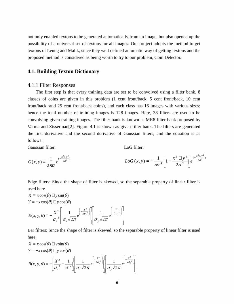
4.1. Building Texton Dictionary 4.1.1 Filter Responses

The first step is that every training data are set to be convolved using a filter bank. 8

classes of coins are given in this problem (1 cent front/back, 5 cent front/back, 10 cent

front/back, and 25 cent front/back coins), and each class has 16 images with various sizes;

hence the total number of training images is 128 images. Here, 38 filters are used to be

convolving given training images. The filter bank is known as MR8 filter bank proposed by

Varma and Zisserman[2]. Figure 4.1 is shown as given filter bank. The filters are generated

the first derivative and the second derivative of Gaussian filters, and the equation is as

follows:

Gaussian filter:

)2

(2

22

2

1),( σ

πσ

yx

eyxG+−

=

LoG filter:

)2

(

2

22

4

2

22

21

1),( σ

σπσ

yx

eyx

yxLoG+

−

��

���

� +−−=

Edge filters: Since the shape of filter is skewed, so the separable property of linear filter is

used here.

���

�

�

���

�

�

��

�

�

��

�

�−=

+−=+=

��

�

�

�−

��

�

�

�− 2

2

2

2

22

2

2

2

1

2

1),,(

)cos()cos(

)sin()cos(

yx

Y

y

X

xx

eeX

yxE

yxY

yxX

σσ

πσπσσθ

θθθθ

Bar filters: Since the shape of filter is skewed, so the separable property of linear filter is used

here.

���

�

�

���

�

�

��

�

�

��

�

�

��

���

�−−=

+−=+=

��

�

�

�−

��

�

�

�− 2

2

2

2

22

24

2

2

1

2

11),,(

)cos()cos(

)sin()cos(

yx

Y

y

X

xxx

eeX

yxB

yxY

yxX

σσ

πσπσσσθ

θθθθ

7

Bar filters:

Edge filters:

LoG filter and Gaussian filter:

Figure 4.1. MR8 Filter Bank

The MR8 filter bank consists of 38 filters but only 8 filter responses. The filters include a

Gaussian and a Laplacian of a Gaussian filter both at scale, 3=σ , and edge filter at 6

orientations and 3 scales and a bar filter also at 6 orientations and the same 3 scales

)}6,2(),3,1(),5.1,5.0{ (),( =yx σσ . The responses of the isotropic filters are used directly, but

the responses of the oriented filters are “collapsed” at each scale by using only the maximum

filter responses across all orientations. Figure 4.2 is a diagram of processing of getting MR8

filter responses.

4.1.2 K-Means Clustering The second step is that using given filter responses, the cluster centers are obtained using

vector quantization algorithm, and in this problem K-means algorithm is used. Since if the

size of given image is 100x100, and we have 8 filter responses, then total 10000 8-vectors

representing only one given image. Therefore, it is expensive and we need to somewhat

reduce the data representation. Leung and Malik[4] noticed that the filter responses are not

totally different at each pixel over the texture, and there should be several distinct filter

response vectors and all others are noisy variations of them. Therefore, K-means approach

can obtain small set of prototype filter responses and the centers of clusters are considered as

representing vector of associated with them. They are called “ textons”.

Variation of classic K-means algorithm used in this problem as follows:

1. Assign k-random cluster centers to the given filter response vectors

2. Assign each pixel to the nearest center. (“nearest” doesn’t mean the physical

distance between the pixel and the center. It means the minimum SSD between

two pixels)

8

3. Re-compute a mean vector of a cluster and set a nearest center to that mean

vector.

4. Iterate 2-3 until it converges.

Figure 4.3 shows the processing of K-means clustering in this problem.

Figure 4.2. MR8 Filter responses

Figure 4.3. Processing of K-means algorithm, K=5 (The small red points are the cluster centers)

9

Those filter responses are all related images, so they are concatenated and clustered to

get K cluster centers, so called textons. In this paper, each class has 16 images, then, total 80

textons will be generated, and these textons are clustered again using K-means to build 5

textons per class; therefore, we have total 40 textons in the dictionary. Now, using these

texton, the statistical learning model is going to be generated. Next section, the detail about

learning models is explained.

4.2. Modeling Statistical Histogram Each class has 4 learning images under various illuminating conditions. They are used to

build one histogram. We have 8 classes, so that 8 probability density histograms will be

generated. In the modeling stage, each pixel of given image is mapped to the nearest texton in

the dictionary we built; hence, each pixel is labeled exactly one texton number, and the

histogram is normalized to build probability density function(PDF). Figure 4.4 shows the

examples of built histogram models.

Figure 4.4. PDFs for learning models

Interesting result is that all histogram graphs of statistical models are similar to each

other, and non-coins’ PDFs are obviously different with them; therefore, we can classify coin

and non-coin images by just comparing two histograms using 2χ distances.

Figure 4.5 shows the examples of PDFs for non-coin images obtained false positive

circles from Hough transform image.

10

Figure 4.5. Non-coin PDF examples

In the next section, we will discuss about classification stage in detail with the

experiment descriptions and results with ROC curve.

4.3. Experiments and Result of Texton Classifier 98 coin images and 88 non-coin images are used in the classification stage. The same

method is applied to those testing images: Each testing image is labeled to the texton number

and normalized the frequency histogram to build PDF, then, this PDF is compared to all

PDFs of 8 classes. If the minimum distance among the 8 PDFs and the testing PDF is less

than a given threshold, then it may be considered as coin, or non-coin image, otherwise. The

following equation explains the classification process.

( )

image.coin of PDF theas considered is then , if

classes) ofnumber (the 8,,1for ,)()(

)()(

1

2

hM

jihih

ihihMINM

N

i j

j

θ<

=��

�

�

�

+−

= =

�

To see the classifier performance, we will use ROC curve along with variation of

threshold θ . The x-axis is false detection rate, and y-axis is correct detection rate with

various thresholds. The following equation is simply representing false rate and correct rate.

set testingin the coins-non ofnumber totalTheclassifier by the determined coins ofnumber The

ratedetection False =

set testingin the coins ofnumber totalTheclassifier by the determined coins ofnumber The

ratedetection Correct =

As we can see Figure 4.6, the best correct rate is about 83% with 15% false detection rate.

We will discuss more about the problems on the result in the next section.

11

Figure 4.6. The ROC curve for the coin classifier of total of 186 testing set with 32 learning images

4.4. Discussion on the Texton Classifier The biggest problem of texton classifier is scale problem as first issued by Varma and

Zisserman[2]. If the sizes of the testing set are significantly different with the sizes of the

learning set, then the correct rate is decreased. And in this paper, we used only one scale

learning images, so the false detection rate might be relatively high as we can see the above

ROC curve. The possible solution for the scale problem is that we can add more learning

images with various scales, but in that case, we have to consider that the statistical learning

model may become various so that correct detection rate can be decreased. The testing

images in this paper are selected from natural images without any scale restrictions, and for

non-coin images, we arbitrary cut circles on parts of testing images to get possible false

positives resulted from the Hough transform. If the scales of images are restricted, then the

performance will be better. We will see the complete output of the restricted images which

are usually seen from the nature in the following section.

The next problem is that the texton classifier needs detail spatial features on testing

images. Because the learning images here have fully detailed spatial structure property, if the

testing images do not have clean texture property, then the classifier tends to not detect those

images.

12

The last problem is that in the natural image, there are relatively many non-coin images

having the same spatial property of coins. Because the texton classifier does not depend on

the color property of coins, the non-coin images with face or small words in them may be

detected as coins.

4.5. Future work for texton classifier Adding more learning images and testing images will help build general statistical model

for coins. To do this, we first have to figure out the problem of scaled images on the texton

classifier.

Bill also has texture property, so it can be expanded to detect bills in the natural images.

5. Final Output

Fig. 5.1 color input image Fig. 5.2 edge image

13

Fig. 5.3 reconstructed from Hough image Fig. 5.4 texton classification applied to Fig. 5.3

6. Contribution

Edge detector: You-Kyung Cha

Hough transform: Young Gyun Yun

Texton classifier: Dong-Shin Kim

Integration and Evaluation: All members

7. References

1. G. Gerig "Linking Image-Space and Accumulator-Space : A New Approach For Object-

Recognition"

2. M. Varma and A. Zisserman. Classifying Images of Materials : Achieving Viewpoint and

Illumination Independence. In Proc. ECCV, volume 3, pages 255-271. Springer-Verlag, 2002

3. Richard O. Duda and Peter E. Hart "Use of the Hough Transformation To Detect Lines

and Curves in Pictures"

4. T. Leung and J. Malik. Representing and recognizing the visual appearance of materials

using three-dimensional textons. IJCV, Dec 1999.

5. S.C. Zhu, C. Guo, Y. Wu, and Y. Wang. What are textons? ECCV, pages 793-807. Springer-

Verlag, 2002