coincidences in the bible and in biblical hebrew (new and ...shor/coincidences in the bible and in...

Coincidences in the Bible and in Biblical Hebrew (New and Old) and

Their Statistical Analysis

Prof. Haim Shore

November, 2011

Copyright © 2011 by Haim Shore

ABSTARCT

An ancient tradition, expressed in numerous examples scattered throughout

various Jewish scholarly works, convey that numerical values of Hebrew words

often represent major physical characteristics associated with the objects that the

words stand for. Simple examples are ―Shanah‖, Hebrew for year, and

―Herayon‖, Hebrew for pregnancy, which have numerical values equal to those of

the duration (in days) of the lunar-based Hebrew year and human pregnancy,

respectively. These examples and many others, all linked to ―counts‖ data, may

be perceived as mere anecdotes. However, recent statistical analysis applied to

a much larger set of examples, comprising subsets of related words with a

common physical trait (measured on a continuous scale), seems to suggest that

there might be more to this tradition than meets the naked eye.

We expound the underlying statistical approach that drove the statistical

analyses introduced in this paper and present some results. Possible criticism is

addressed and discussed.

Keywords: Biblical Hebrew, Chazal, linear transformation, linear regression,

Midrash Rabbah, statistical textual analysis

2

1. INTRODUCTION

An ancient Jewish tradition assumes the existence of hidden linkages between

physical properties of ―entities‖ of the real world and respective biblical verses or

biblical Hebrew words, related to these entities. This conviction is expressed not

merely by general assertions, like ―Bezaleel knew how to assemble letters with

which heaven and Earth had been created‖ (Talmud, Berachot, 55a), but also in

various detailed examples, often reflecting efforts to extract real (occasionally

useful) information about the physical world from analysis of the structure and the

numerical values of related words, or verses, in the Hebrew Bible. For example,

the numerical value of the Hebrew ―Heraion‖ (pregnancy; Hoshea 9:11)

represents the expected duration of human pregnancy (271 days; Midrash

Rabbah, Bereshit, 20). Also therein, Rabbi Shmuel relates to a verse from the

Bible: ―Harbeh arbeh itzvonech ve-heronech‖ (―I will greatly multiply the pain of

thy child bearing‖, Gen. 2:16). Since ―Harbeh‖ (―greatly‖) is numerically equivalent

to 212, an embryo surviving 212 days, thus Rabbi Shmuel, will probably survive

the whole pregnancy.

Some further examples, relating to ―counts‖ data, are given in Table 1.

Insert Table 1 about here

While these examples and many others may be perceived as a collection of

anecdotes (―cherry picking‖, in statistical parlance), recent statistical analysis

conducted on a much wider scale, referring to data measured on continuous

scales, seems to suggest that this tradition may have deeper roots in reality than

initially and intuitively suggested by the documented Jewish oral and written

tradition.

A first serious attempt to subject these ―facts‖ of tradition and faith to serious

statistical analysis had been carried out in Shore1, where various sets of related

words, bound together by a shared physical trait (or traits), were analyzed. These

included, for instance, primary colors and their respective spectral frequencies,

metals and their atomic weights and specific heat capacity of the three phases of

water (ice, liquid water and steam; refer to Section 3.3). Some of these examples

3

were made public in an interview given by the author to the Israeli daily The

Jerusalem Post (December, 4, 20092).

An innovative aspect of the examples assembled in Shore1 is the introduction of

statistics and statistical hypothesis testing to establish in a rigorous scientifically

acceptable fashion existence of a relationship between the numerical values of a

set of inter-related biblical Hebrew words and a major physical property shared

by all objects that these words stand for. As explained in detail later, existence of

a statistically significant linear relationship (either on the original scale of the

physical trait or on a log scale) may indicate that the numerical values of the

words in the set deliver same information as the scientifically proven physical

measure (even though the latter is given on a different scale).

In this article, we first explain in Section 2, via a parable, why a linear relationship

between two sets of observations, collected by two measuring devices possibly

operating on different scales, indicate that the two sets of observations deliver

identical information. While this may seem self-evident and redundant to readers

trained in the exact sciences, it may not be so for other readers. Therefore a

numerical example is introduced, given in the form of a parable. In Section 3 we

present four simple preliminary examples for the existence of linear relationships

between numerical values of inter-related biblical Hebrew words and a related

physical trait. A computer simulation study examines, for one example, how

probable are the results obtained if the respective Hebrew words were generated

randomly by the computer. Section 4 expounds the major example of this paper,

which focus on the nine planets (including Pluto, which has recently been deleted

from the list of recognized planets). All biblical Hebrew words that indisputably

relate to celestial objects are examined in relation to three physical traits of the

planets: diameter, mass and orbital angular momentum (OAM). ‎The main reason

for selecting this example is the large number of points in the set (nine). Aligning

nine points on a straight line accidentally is highly improbable, and renders it

extremely hard to relate to this phenomenon as mere coincidence. This example

is followed, in Section 5, by new findings obtained after publication of the book1,

either by us or via comments and suggestions received by e-mail from readers

4

exposed to the book1 or to the interview in the Jerusalem Post2. Section 6

addresses possible criticism of the validity of the phenomenon presented here

and its statistical analysis.

To assist the reader, who may wish to monitor more closely how the numerical

examples in this paper have been analyzed, Table 2 presents a list of Hebrew

letters and their traditional numerical values.


2. A PARABLE (all facts imaginary; conclusions valid)

At the beginning of the twentieth century, an archeological excavating expedition

arrived to the Holy Land to carry out some research in the vicinity of the city of

Jericho. A while into the beginning of the excavation, a papyrus was exposed

that contained a series of twenty numbers. These are given in Table 3a (denoted

―First set‖).

Insert Table 3a about here

No caption explained what the numbers meant so the mysterious papyrus was

stored in a secured place and excavation continued. A while later, a second

papyrus was revealed, with a second list of numbers (of same size as before;

refer to Table 3b).

Insert Table 3b about here

However, this time the caption gave exact details of the nature of these numbers

and when they were collected. It read: ―Temperatures measured at this site for

twenty consecutive days in the year 150 BC‖. Researchers were delighted and

they had no doubt that this is an authentic document; however they were still at

loss explaining the numbers in the first document, even after consulting the best

available statisticians of the time. Several months later, a young archeologist

from the expedition came up with a brilliant idea: Perhaps the numbers in the first

document are measurements of same temperatures as specified in the second

document. After some scholarly arguments and mutual convincing, the team

decided to test this hypothesis statistically.

5

How could the new hypothesis be tested?

Figure 1 plots the two sets.

Insert Fig. 1 about here

A linear relationship is obvious. Linear regression analysis gave the following

equation (F- Fahrenheit, C- Celsius):

F = 32 + 1.8 C

Data analysis indeed validated the young archeologist’s choice of method to

resolve the mystery surrounding the first set of numbers.

3. FOUR PRELIMINARY EXAMPLES

In this section we introduce four examples (subsections 3.1-3.4), all sharing two

important characteristics: each example addresses a set of three biblical words

for which no controversy exists about their true meanings, and nearly all words in

these examples are unique in the sense that there are no synonyms in biblical

Hebrew that may substitute these words.

In subsection 3.5 we present a computer simulation study, relating to one of the

examples, that examines how likely it is for a trio of Hebrew words, generated

randomly by the computer, to be aligned in a linear configuration close to that

shown in the example.

The appendix details calculation of the numerical values of Hebrew words that

appear in the first three examples of this section.

3.1 Cyclic Time-periods: Day, Month, Year (“Yom”, “Yerach”, “Shanah”)

―Periodicity‖ is a major physical property that differentiates between the time-

periods that the words above stand for. To check whether numerical values of

Hebrew words represent periodicity affiliated to these words, one has to express

periodicity (or frequency) by a common measurement unit. For example, if we

chose ―Cycles per year‖, then the periodicity of ―Day‖ would be: (29.53059*12) =

354.37 (the lunar month, on which the Hebrew calendar is based, is on average

29.53059 days); the periodicity of ―month‖ will be 12 and that of ―year‖ 1. If ―Day‖

6

served as the measurement unit, then the frequency of ―Year‖ will be 1/354.37

cycles per day. In this example we adopt a unit commonly used in science and

engineering to denote frequency of cyclic phenomena, namely, Hertz (1 Hertz is

one cycle per second). Note, that in regard to the results derived from the

statistical analysis, the actual unit selected is inconsequential provided use of this

unit is consistent throughout the statistical analysis.

Table 4 displays numerical values of the words in the set and the frequency (in

Hz) associated with the ―object‖ that each word stands for.


The reader should be reminded that a numerical value can be represented by

any system, for example, the decimal system. Alternatively, a number may be

expressed as a power value. Thus, "7" can be represented in two modes: 7 =

100.8451. The number 0.8451 is denoted ―the log of 7 to the base of 10.‖ In fact,

when numerical values in a sample of observations span several orders of

magnitude, it is customary in science and engineering to represent these

observations, for statistical modeling, by their log values. This is implemented

with respect to nearly all examples in this paper (with Example 3 in Section 3.3

as the sole exception, due to the proximity of the values of the response

variable).

Figure 2 displays the three points whose values are displayed in Table 4. On the

horizontal axis numerical values of the Hebrew words are registered (Duration

Numerical Values, or DNV), and the vertical axis displays the respective values

of frequency, on a natural log scale (log scale to the basis of ―e‖).


We realize that the points align themselves on a straight line with a linear

correlation of -0.9992 (a value of -1 would have been expected for an exact

(mathematical) decreasing linear relationship). The actual statistical significance

level is 2.5%, below the commonly accepted threshold value of 5%.

3.2 Diameters of Moon, Earth, Sun (“Yareach”, “Eretz”, “Shemesh”)

7

This example examines whether the Hebrew moon, Earth and sun bear any

relationship to a major physical trait of these celestial bodies, namely, their

equatorial diameters. As in the earlier example, due to variation in orders of

magnitude of the diameters they will be registered in the plot on a log scale.

Table 5 introduces the data (diameters taken from NASA site), and Figure 3

displays the data, with numerical values of the Hebrew words (Object Numerical

Value, or ONV) on the horizontal axis and the respective diameters, on a log

scale, on the vertical axis.



The phenomenon evidenced in the earlier example is repeated: the three points

align themselves on a straight line with a linear correlation of 0.999 (a value of 1

would have been expected for an exact (mathematical) increasing linear

relationship). The actual significance level obtained is comparable to that of the

former example (2.9% vs. 2.5% for the first example). Note that significance

values obtained for larger data sets are expected to be smaller, as indeed we

may find out in Section 4 (with sample size n=9).

3.3 Specific Heat Capacity of the Three Phases of Water: Ice, liquid water,

steam (“Kerach”, “Mayim”, “Kitor”)

Heat capacity, or thermal capacity, is the ability of matter to store heat. The heat

capacity of a certain amount of matter is the quantity of heat (measured in joules)

required to raise its temperature by one Kelvin. SI denotes the International

System of Units. The SI unit for heat capacity is J/K (joule per Kelvin).

Specific heat capacity (SHC) of a substance is defined as heat capacity per unit

mass. It is commonly denoted by symbols like c or s, and occasionally called just

specific heat.

The SI unit for SHC is joule per kilogram Kelvin, J·kg-1·K-1, or J/(kg·K). This is the

amount of energy (heat) required to raise the temperature of one kilogram of the

substance by one degree Kelvin.

8

The symbol cp is often used to denote SHC at constant pressure.

Substances with low SHC, such as metals, require less input energy to increase

their temperature. Substances with high SHC, such as water, require much more

energy to increase their temperature. The specific heat can also be interpreted

as a measure of how well a substance preserves its temperature (i.e., ―stores‖

heat—hence the term ―heat capacity‖).

Water is often used as a basic standard relative to which SHC values are

compared. However, the water’s SHC depends on which state it is in. Frozen

water (that is, ice), liquid water, and gaseous water (that is, steam) have different

SHCs. In fact, this is the major physical trait that differentiates between the three.

Table 6 displays SHC at constant atmospheric pressure for all three states of

water, measured in J/(kg·K). SHC for ice and steam were naturally recorded at

transition temperature from one phase to another.



The biblical Hebrew words for the three water phases are ―kerach‖ (ice), ―mayim‖

(water) and ―kitor‖ (steam). Their numerical values also appear in Table 6 as

WNV (Water Numerical Values; refer to the appendix for how these were

calculated).

Linear regression analysis was applied with water’s SHC values as the response

(the dependent variable) and WNV values as the regressor (the independent

variable).

For sample size n=3, the linear correlation coefficient is 0.9995. The model F-

ratio is 917, which at the 5% level is significant (p<0.0210).

The original observations with the fitted regression equation and 95% confidence

limits are shown in Figure 4. For easy identification, the WNV value is given atop

each observation. Predicted values may be easily calculated from the regression

equation included in the plot’s caption.

9

3.4 Velocities

In this subsection we address two sets of Hebrew words, each comprising three

words, that are associated with velocities. The first trio of words is {Light, Sound,

Standstill}, the second {Rainbow, Thunder, Silence}. Curiously, the last word in

the two sets is represented in Hebrew by a single word that delivers both

meanings (namely, standstill and silence). Table 7 presents the two sets, with

their associated numerical values (VNV-Velocity Numerical Value) and the

associated actual velocities (V, in meter/second). For sound (and thunder) we

took the standard sound speed in air at normal atmospheric pressure and 25C.

Other values (suitable for other conditions) can be taken without practically

affecting the results of the statistical analysis (since the latter is conducted on

response values measured on a log-scale). For standstill (silence) we took

velocity to be 1, so that on the log-scale, in which the statistical analysis is

conducted, we obtain for log-V a value of 0.

Figures 5 and 6 show the fitted linear regression models, with the associated

95% confidence intervals. Figure 7 displays plots of the joined points in each set,

for both sets. It is indeed unexpected that both sets converge at the same

Hebrew word ("Dmamah").


Insert Figs. 5-7 about here

3.5 A Computerized Simulation Experiment

In this subsection we examine how likely it is for a trio of Hebrew words to be

arranged on a straight line, given the velocities of the previous example. To

assess that probability, we used computerized simulation, where ten thousands

sets of three words had been randomly generated. In each set the first word

comprised four letters (as in Dmamah) and the other two words comprised three

letters each. Letters were selected with probabilities proportional to the relative

frequencies of the letters in the Hebrew Bible. Also, if a word comprised three or

more repetitions of same letter it was discarded and another random word

10

generated (it is impossible to have a Hebrew word of three or four letters that

comprises 3-4 repetitions of same letter). The response variable (the measure

subjected to statistical analysis) was the ratio of the slopes (SR) of the two lines

that connect two adjacent points, namely:

3 2 3 2

2 1 2 1

( ) / ( )

( ) / ( )

Y Y X XSR

Y Y X X,

where Yj (j=1,2,3) is the value on the vertical axis of the j-th point and Xj is the

value on the horizontal axis of the j-th point (j=1,2,3). It is assumed that the points

are sorted according to their Y values in an ascending order. Thus, generated

word that represents Dmamah is the first point (j=1) and so on.

Obviously for three points that are arranged on a single line (whether the line has

positive or negative slope) we will have (ideally) SR=1. For three-point sets that

are arranged near a straight line we will have SR values around 1.

It can be easily established from Table 7 that for the two sets discussed in

subsection 3.5 we obtain:

SR1 =1.550 for {Or, Kol, Dmamah}

SR2 = 1.056 for {Keshet, Raam, Dmamah}.

Analyzing the sample (N=10000 sets of three words each), we obtain for SR:

Mean = -1.6725 ; Standard Deviation = 69.16

Figure 8 displays a histogram of the sample.

Insert Figure 8 about here

The figure shows that SR is indeed normally distributed. Assuming this

distribution, we obtain, with the above estimates of the mean and standard

deviation:

Pr[0.4<SR<1.6]= 0.006917 ; Pr[0.9<SR<1.1]= 0.001153 ;

(intervals were selected to be symmetrical around SR=1 and to include SR1 and

SR2)

11

Thus, the probability that a randomly generated set of three Hebrew words, with

configuration similar to that used in the example, will fall in the intervals specified

(where we have obtained SR1 and SR2) is less than 1% for both sets of words.

Furthermore, these probabilities were calculated without filtering out (excluding)

sets of words that do not have any Hebrew meaning. If this would have been

done (a prohibitive undertaking for a sample that large) the probabilities would

have been even smaller.

4. PRIMARY EXAMPLE: THE PLANETS

4.1 Planetary Diameters

This example examines existence of a possible link between names for celestial

objects that appear in the Bible and known diameters of the planets. This is an

outrageous and hard to prove (let alone believe) proposition on two counts. First,

the Bible never refers to any particular planet (apart from Earth, which for

obvious reasons is never considered in the Bible to be one of a set of planets).

Secondly, why should one even conceive of biblical sky-related names to be

associated with planets’ diameters? Furthermore, given that there is no allusion

to planets, how would one link a particular biblical name to a particular planet?

We are unaware of any scholarly interpretation that attributes apparently celestial

biblical names to specific planets. However, certain names are traditionally

interpreted to be associated with groups of stars or just representing a planet (no

attribution attempted). Examples are Ash, Aish, Ksil and Kimah (we will refer to

these shortly). The most commonly accepted Even-Shoshan Hebrew

concordance4 interprets Ash to be one of the planets, Aish to be a group of non-

moving stars (―Kochvei-Shevet‖), Ksil to be the group of stars called Orion, and

Kimah as ―A group of radiating stars of the sign Taurus‖.

We now discard these traditional interpretations, and make an initial assumption

that all references to celestial objects in biblical Hebrew relate to planets

(excluding the sun and the moon, which are also celestial objects denoted by

specific Hebrew words). There are five such names: Kimah (Amos 5:8; Job 9:9,

38:31), Ksil (Isa.13:10; Amos 5:8; Job 9:9, 38:31), Ash (Job 9:9, occasionally

12

also Aish, Job 38:32) and Teman (Job 9:9). The latter means in biblical Hebrew

also south, but from the general context of the verse where it appears Teman

obviously relates to a celestial object and so it is interpreted by Jewish biblical

scholars. We add to this set Kochav, which in biblical Hebrew simply means star.

Kochav is assumed here to relate also to an unknown planet, though in most

places in the Bible it appears in the plural to signify all stars or any star. Such

developments, where a specific meaning is later generalized, is often

encountered in the evolution of languages (relate, for example, to the words ―to

xerox‖ or ―fridge‖). We assume that same destiny befell Kochav.

Two other names added to the set are Mazar (only the plural, Mazarot or

Mezarim, appear in the Bible, at Job, 38:32 and Job 38:9, respectively), and

―Shachar‖. The first (Mazar) is interpreted in Even-Shoshan4 as Mazal (a planet,

in both ancient and modern Hebrew). The second is often interpreted by Jewish

scholars as ―a morning star‖ (relate, for example, to SofS. 6:10, and how Jewish

commentators interpret it). As elaborated on at some length in Shore1, these

names probably represented originally the two most luminary stars in the sky,

after the sun and the moon, namely, Venus (probably named Mazar in Hebrew)

and Jupiter (probably named Shachar in Hebrew). As we shall later demonstrate,

the statistical analysis indeed corroborates this interpretation for the two names.

We now have nine biblical names for celestial objects (including Earth). Apart

from the latter, which planets do these names possibly allude to?

For no obvious alternative method to assign names to planets, we sort in an

ascending order the numerical values of the biblical Hebrew names (denoted

ONV for ―Object Numerical Values‖), and likewise for the nine planets’ equatorial

diameters (as given by NASA site, including also Pluto that had recently being

omitted from the list of planets). Table 8 displays the results.


The most surprising finding in this table is that the words Mazar and Shachar

indeed occupies in the sorted list same ordinal positions as the very same

planets that these names have formerly been attributed to from altogether non-

13

statistical arguments (refer to Shore1, sections 8.3.4 and 8.3.5). Also Earth

occupies same positions in both of the sorted lists. We conclude that this

convergence to identical ordinal positions, emanating from two different modes of

analysis, corroborates the validity of the analysis on which this table rests.

Plotting the planets’ diameters on the vertical axis and ONV values on the

horizontal axis, Figure 9 is obtained.


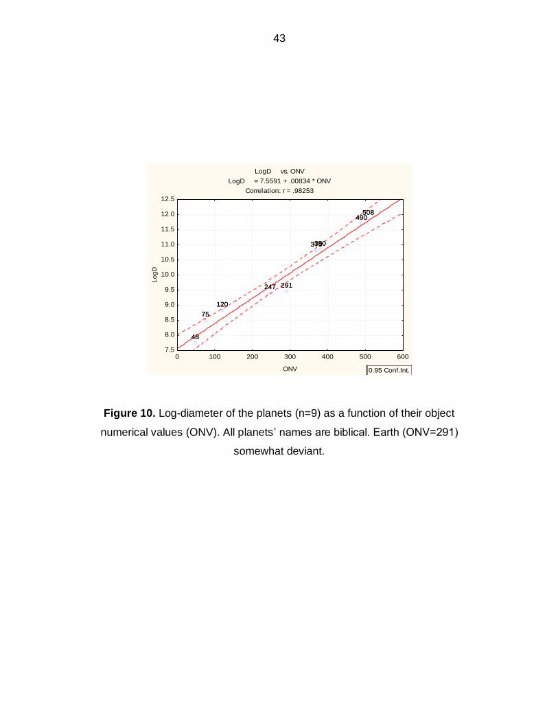
A nonlinear relationship is evidenced by the plotted points. Proceeding as in the

previous example (namely, plotting diameters on a log scale) we obtain Figure

10.


A linear relationship surfaces, unexpectedly and with no logical explanation.

Statistical linear regression analysis was applied to the entire sample of nine

points to ascertain whether the linear relationship is significant. For the present

analysis (n=9), we have obtained a correlation value of 0.9825. The model F-ratio

is 195.2, which is highly significant (p<0.000002).

Confidence interval limits (at 95% confidence) are also plotted in Figure 10. We

realize that Earth (ONV=291) resides somewhat below the lower confidence limit.

Therefore the previous analysis is re-run, excluding Earth. Results are plotted in

Figure 11.


With n=8, the R value is now 0.9919, the model F-ratio has jumped to 367

(formerly 195.2), which is highly significant (p<0.000001).

4.2 Planets’ Orbital Angular Momentum (OAM)

The idea for this analysis was forwarded to me by Dr. Howard Sharpe of Canada.

Assembling of data and analyses performed are the author’s.

One of the most significant characteristics of a planet’s orbit is its orbital angular

momentum (OAM). The latter is defined as the product of the planet’s mass

14

times the planet’s average distance from the sun times the planet’s average

orbital speed:

L = M*R*V = M(2R2) / T

where M is the planet’s mass (kg), R its average orbital radius (meters), V its

orbital linear speed (meters per second) and T its orbital period (in seconds).

Table 9 displays Hebrew words’ numerical values (ONVs, as in Table 8) together

with planets’ OAM values (kg*m2/sec; m is ―meter‖), both in their original and their

log values.


On comparison of Tables 8 and 9 we realize that only Neptune and Uranius

could not have maintained their original ordinal positions (as given in Table 8) if

sorted according to their OAM values. The mass density of Neptune (1.76 g/cm3)

is larger than that of Uranius (1.30 g/cm3), however the equatorial radius of the

latter (25,559 km) is larger than that of the former (24,764 km). Both equatorial

radius and mass density affect OAM (as evidenced by the formula above). It is

therefore not necessary that nearly all planets in Table 9 (with Uranius and

Neptune excepted) should have preserved their sorted positions both with

respect to equatorial diameter and to OAM. Due to the proximity in both size and

OAM of Neptune and Uranius we have decided to preserve in Table 9 same

ordinal positions for all planets as given in Table 8.

Figure 12 displays the results (the vertical axis presents log-OAM).


We realize that all nine points align themselves on a straight line. The adjusted -

squared ( is correlation) is 0.958. The model F-ratio is 181.8, which, for n=9, is

highly significant (p<0.000003). Since Earth point is somewhat deviant (below the

confidence interval lower limit) it is removed from the sample, and linear

regression analysis is re-run for a sample of n=8. The adjusted -squared is

0.977. The model F-ratio is 294.3, which, for n=8, is highly significant

(p<0.000003). The results are presented (with Earth excluded) in Figure 13.

15


4.3 Planets’ Mass

Planets’ diameters and planets’ masses, both measured on a log scale, should

be linearly inter-related if their mass densities were equal. However, we know

that average mass densities of planets differ (relate to Table 8). Therefore,

values of planets’ masses are added to Table 9, and we explore the relationship

between ONV values and the respective planetary mass for all nine planets.

Figure 14 displays the results.


A linear relationship is evidenced by the plot. Applying linear regression analysis,

the adjusted -squared is 0.953. The model F-ratio is 161.8, which, for n=9, is

highly significant (p<0.000004).

5. SOME FURTHER NUMERICAL EXAMPLES

Examples in this section, though numerical, are not accompanied by statistical

analysis. Since they lend support to the main claim of this article, they are added

here as further instances for the realization of the characterization delineated in

the Introduction.

5.1 How Long is Human Pregnancy?

The data below were forwarded to me by an American Obstetrician/Gynecologist,

living and working in Mali, West Africa. Permission was granted to publicize

excerpts from his e-mails, as given below. However he preferred to remain

anonymous and therefore we will refer to him as Dr. X.

His e-mail to me regards the duration of human pregnancy. In my book I quote

the numerical value of 271 days for ―Herayon‖ (pregnancy), as indicative of

expected duration of human pregnancy (Shore1, p.49). However I quote two

commonly accepted methods to calculate duration of human pregnancy: ―One

method is to measure human pregnancy from fertilization time, which is

commonly accepted to be, on average, 266 days. Another method is to measure

16

human pregnancy from the last menstrual period, which is commonly accepted

as 280 days. The simple average (midpoint) between these two figures is 273

days (about nine months).‖

Thus write Dr. X in his e-mail:

―Dr Nagele, a physician in the 1850’s or so, created a rule for estimating the due

date of a human pregnancy based on the first day of the last menstrual period.

At this point, no one even knew that ovulation and therefore conception was

taking place at approximately day 14 of the ovulatory cycle, so the only fixed

point was the first day of the last menstrual cycle, and of course, one is not

pregnant at this point, as one is actively sloughing the endometrial contents.

Nevertheless, this is the one fixed point by which to date a pregnancy, and in his

study of patients, he determined that the due date is 280 days after the first day

of the woman’s last menstrual cycle. He invented a rule by which to estimate this

for patients. It is still used today ─ Nagele’s rule5. Take the first day of the last

cycle and then subtract three calendar months and add 7 days─ the resulting day

(about 280 days later) will be the patient’s approximate due date.

Later, in the 1930’s or 40’s it was determined6 that ovulation, and therefore

conception, was taking place approximately 14 days after the first day of the last

menstrual period. Thus the classic length of human gestation of 266 days after

ovulation (and therefore conception, plus or minus one day, as both the sperm

and the egg can live in the female genital tract for about one day in the

unfertilized state, before dying) was established.

These two numbers have been used ever since, and you refer to them in your

book. However, in 1990, Dr Robert Mittendorf et al. published a comprehensive

study of estimated delivery dates of American women7. As far as I know, this is

the most recent scholarship done on this question. Interestingly he found that for

women who had never had a child before, the average length of pregnancy was

274 days after conception, while for women who have had at least one baby

before, the average length of gestation was 269 days. I find it fascinating that the

17

average of these two is 271.5!! It is remarkable to me that 271 is found to be so

near the center of the distribution by the most recent scholarship.

Thus Dr Mittendorf’s data show average gestation to be about 5 days longer on

average than Dr Nagele’s data, and this only serves to further tighten the biblical

evidence for 271. I suspect a true picture of the data would show a bell shaped

curve centered directly on 271.‖

5.2 What Percentage of Human Blood is Cellular?

In the same message, Dr. X refers to the fact that blood in Hebrew (―Dam‖) is

numerically equivalent to 44. I refer to this fact in my book, drawing attention that

whenever a numerical value of a biblical Hebrew word amounts to a repeated

appearance of a single digit (like ―Sheleg‖, snow, equaling 333), this number

indicates a major physical property of the object that the word refers to. Relating

to human blood, I have interpreted the repeated ―4‖ as signaling the number of

human blood varieties that exist (Shore1, p. 61 and 146). Dr. X believes that the

number ―44‖ conveys an even deeper meaning, signaling the proportion of

cellular blood (all the rest is liquid) in the human blood:

―One other thing that strengthens your case is the fact that one standard

measure of human blood is called the hematocrit. This is the percentage of

blood that is cellular (the rest being liquid- the plasma). The hematocrit normal

values vary between males and females, but normally they are cited to be 42 -

50% for men and between 35 - 47% for women. Consult any laboratory manual

and you will see that the norms cited for male and female hemoglobins always

contain the number 44 for both, and a simple average of the male and female

norms will always center around 44!!! I looked at several different limits of

normal according to different texts and sites, and found my averages to always

be between 42.5 and 45. So…this is astounding, eh?? 44 is definite ly a key

number for human blood.‖

18

6. POSSIBLE CRITICISM AND A DISCUSSION

In this paper we have demonstrated a certain phenomenon, rooted in Jewish

culture and tradition, namely, that traditional numerical values of Hebrew words

store information that directly relates to a major physical trait of the objects that

the words are linked to. Few of the examples given here are a subset of a wider

sample given in Shore1, though with no statistical detail as expounded here. In

this section we elaborate on some possible criticism that may be raised regarding

the main claim of the paper, both in terms of the plausibility of the claim and the

supportive evidence.

A first argument is that human language, being human, cannot include

information unknown to generations past, and therefore this phenomenon is a

mirage. People of faith would respond that not all human languages are of

human origin, and if Hebrew, the original language of the Old Testament, is of

divine origin─ then this phenomenon is possible. Attempting to avoid arguments

of a religious nature, we believe that such debate should be averted and only the

data, supported by adequate statistical analysis, should be the basis for a proper

assessment of the phenomenon addressed in this article.

A second argument relates to the fact that not all Hebrew words succumb to the

characterization given in this article, namely, they are not all connected to some

related major physical trait. A good example is the link between colors ’ names

and color wave frequencies, an analysis that was addressed in the Jerusalem

Post interview (alluded to earlier). In this example, I have shown that biblical

Hebrew names of a subset of five colors have sorted numerical values that

preserve same order as their respective wave frequencies, a finding that has low

probability (1/120) of occurring by chance. In my book I enumerate 24 names of

colors in the Hebrew language, most of which appear also in the Bible. Why were

only five colors selected? The answer is twofold: first, with a single exception

only primary colors were selected for the sample (explanation why only primary

colors could be analyzed and why an exception to this rule was included in the

analysis is given in Shore1); of the seven primary colors only four are mentioned

19

in the Bible and they were all included in the sample. Secondly, Hebrew being an

ancient language, not all words in the Bible have meanings that are known to us

today or that cannot be debated. Therefore, only words that have obvious and

unchallenged meanings could be included in the sample. Considerations like

these may apply to other analyses. Another argument raised is that the

phenomenon addressed in this article (and in my book) is not all-inclusive,

namely, a linear relationship cannot be established for all sets of Hebrew words

with a common physical trait. The response to this argument is that human

languages evolve overtime and in the process they absorb words from other

languages, where the phenomenon simply does not exist. Furthermore, one

cannot impose his, or her, desire on how pervasive the studied phenomenon

should be. One should accept this phenomenon as it is and make do, regarding

its validity, with the extremely small probability of its occurring randomly (as

shown in this article and elsewhere). No theoretical argument can condition the

reality of an observed phenomenon on its being all inclusive, ―or else it does not

exist‖.

A third argument relates to the examples as ―cherry picking‖. This argument is

serious and cannot be dismissed. To repudiate it, a certain critical mass of

examples, with a large enough sample size (as shown in Section 4) and

corroborated by proper statistical analysis, should exist that provides ample

cumulative evidence that renders the phenomenon real even to the eye of the

most skeptic.

We believe that such a threshold has been surpassed. Others may disagree.

REFERENCES

[1] Shore, H. (2007). Coincidences in the Bible and in Biblical Hebrew. iUniverse,

NE. USA

[2] Author’s interview at the Jerusalem Post (Dec., 4th, 2009; Accessible also via

the book’s Amazon USA site): Author's interview for the Jerusalem Post

http://fr.jpost.com/servlet/Satellite?cid=1259831450363&pagename=JPost%2FJPArticle%2FShowFull

20

[3] Shore, H. (2009). Is there hidden information in biblical Hebrew? Free

download from author’s personal web-site at:http://www.bgu.ac.il/~shor/index.htm

[4] Even-Shoshan (1988), A. New Concordance for Torah, Neviim, and Ketuvim.

Revised edition. Jerusalem: Kiriat-Sefer.

[5] The information about Dr Naegele is available on Wikipedia under the

heading of Naegele's Rule.

[6] O'Dowd M, Phillip E (1994). The History of Obstetrics and Gynecology.

Parthenon Publishing Group, , p. 259

[7] Mittendorf R, Williams MA, Berkey CS, Cotter PF. The Length of

Uncomplicated Human Gestation. Obstet Gynecol 1990;75:929-32. PMID

2342739.

http://www.bgu.ac.il/~shor/index.htm

http://www.ncbi.nlm.nih.gov/pubmed/2342739

http://www.ncbi.nlm.nih.gov/pubmed/2342739

21

Appendix

Calculation of numerical values of Hebrew words for the examples in Section 3.

Example 1 (Section 3.1): Values of DNV (Table 4)

Yom (day):

66( = 01 = ם( + )6 = ו( + )01 = י)

Yerach (month):

008( = 8 = ח( + )011 = ר( + )01 = י)

Shanah (year):

066( = 6 = ה( + )61 = נ( + )011 = ש)

Example 2 (Section 3.2): Values of ONV (Table 5)

Yareach (moon):

008( = 8 = ח( + )011 = ר( + )01 = י)

Eretz (Earth):

000( = 01 = ץ( + )011 = ר( + )0 = א)

Shemesh (sun):

601( = 011 = ש( + )01 = מ( + )011 = ש)

Example 3 (Section 3.3): Values of WNV (Table 6)

Kerach (ice)

018( = 8 = ח( + )011 = ר( + )011 = ק)

Mayim (water)

90( = 01= ם ( + )01= י ( + )01= מ )

Kitor (steam)

006= (011 = ר) + (6 = ו) + (0 = ט) + (01 = י) + (011 = ק)

22

List of Tables

Table 1. Numerical examples (with ―counts‖ data) for matches between

numerical values of biblical Hebrew words and corresponding values of related

major physical traits

Table 2. Hebrew letters and their traditional numerical values (letters in brackets

appear only at the end of the word and occasionally given different numerical

values; not here).

Table 3. Two sets of measurements reported by the excavation delegation

(Section 2).

Table 4. Data for analysis of frequencies (in Hz, cycle per second)

for ―day, month, year‖.

Table 5. Actual and predicted diameters of the moon, Earth and the sun (based

on ONV, the numerical value of the Hebrew names).

Table 6. Specific heat capacity, Cp (at constant atmospheric pressure) for water

in its various phases (in joule per kilogram per 1 degree Kelvin) with respective

numerical values of the biblical Hebrew names, WNV (water numerical values).

Table 7. Data for two sets of Hebrew words: {Or, Kol, Dmamah} (light, sound,

standstill) and {Keshet, Raam, Dmamah} (Rainbow, thunder, silence). Response

variable is velocity (in meter/second, on a log scale), associated with these

words. For "Dmamah" a value of 1 is selected so that it becomes zero on the log-

scale.

Table 8. Data for equatorial diameters and mass densities of planets with their

assumed biblical names and their numerical values (―Object Numerical Values‖-

ONV)

Table 9. Data for planetary orbital angular momentum (OAM) with assumed

biblical names and their numerical values (ONV).

23

Table 1. Numerical examples (with ―counts‖ data) for matches between

numerical values of biblical Hebrew words and corresponding values of related

major physical traits

* These examples are a small set from a larger sample; however, not all names

in biblical Hebrew succumb to this linkage, mainly because only rarely does a

single number of chromosomes characterize all branches of a given species.

No.

Biblical Hebrew

word (English)

Num. value of Hebrew word

Associated physical

trait

Num. Value of physical Trait

Source Example quoted

in:

"ה.נ.ש" 1

(―Shanah‖, Year)

355 Duration (number of

days) of lunar-based

year

29.530589X12= 354.3671

Average lunar month (from NASA

site)

Ref. 1,

p. 241

"ד.י" 2

(―Yad‖,hand)

14 Number of bones in

human hand

14 Common knowledge

Ref. 1,

p.149

"ן.ו.י.ר.ה" 3

(―Heraion‖, pregnancy)

271 Duration (number of

days) of Human

Pregnancy

273 or 271.5 Refer to

Section 6.1

in this paper

Midrash Rabbah (Ref. 1, p. 49)

"ם.ד.א" *4

(―Adam‖, human being)

45 Number of chromosomes common to

all human beings

45

(23 pairs, one sex chrom. different for male and female)

Common knowledge

No prior referenc

e

"ל.מ.ג" *5

(―Gamal‖, camel)

73 Number of chromosomes common to

all camels

73

(37 pairs, possibly one sex chrom. different for male and female)

Site: Answer.com

No prior referenc

e

"ד.ל.ח" *6

(―Choled‖, rat)

42 Number of chromosome

s

42

(21 pairs)

Site:

wikipedia.org

No prior referenc

e

http://en.wikipedia.org/wiki/

http://en.wikipedia.org/wiki/

24

Table 2. Hebrew letters and their traditional numerical values (letters in brackets

appear only at the end of the word and occasionally given different numerical

values; not here).

Letter Numerical value

Name (English)

Name (Hebrew)

Pronounced as

A אלף alef 1 א

B or V בית bet 2 ב

G גימל gimmel 3 ג

D דלת dalet 4 ד

H הא hei 5 ה

V וו vav 6 ו

Z זין zayin 7 ז

German Ch חית chet 8 ח

T טית tet 9 ט

Y (I) יוד yod 10 י

(ך ) כ 20 kaf כף K or German Ch

L למד lamed 30 ל

(ם ) מ 40 mem מם M

(ן )נ 50 nun נון N

S סמך samech 60 ס

A עין ayin 70 ע

(ף ) פ 80 peh פה P, Ph or F

(ץ ) צ 90 tzadi צדי Tz

K or Q קוף kof 100 ק

R ריש resh 200 ר

Sh or S שין shin 300 ש

T תו tav 400 ת

25

Table 3. Two sets of measurements reported by the excavation delegation

(Section 2).

3a. First set

3b. Second set

1 2 3 4 5 6 7 8 9 10

80.6 87.8 68 57.2 62.6 78.8 50 57.2 80.6 55.4

11 12 13 14 15 16 17 18 19 20

62.6 71.6 80.6 93.2 59 53.6 62.6 71.6 86 91.4

Temperatures measured at this site for 20 days in the year 150 BC

No. 1 2 3 4 5 6 7 8 9 10

Tem. 27 31 20 14 17 26 10 14 27 13

No. 11 12 13 14 15 16 17 18 19 20

Tem. 17 22 27 31 15 12 17 22 31 33

26

Table 4. Data for analysis of frequencies (in Hz, cycle per second)

for ―day, month, year‖.

Name DNV Frequency Log frequency

Day (“Yom”) 56 1.1574E-05 –11.3667

Month (“Yerach”) 218 3.9194E-07 –14.7521

Year (“Shanah”) 355 3.2661E-08 –17.2371

27

Table 5. Actual and predicted diameters of the moon, Earth and the sun (based

on ONV, the numerical value of the Hebrew names).

Name Diameter

(actual, km) Log-diameter

ONV

(Object Numerical Value)

Diameter

(predicted)

Error

(%)

Moon 3474.8 8.153292 218 3946.75 13.6

Earth 12756.28 9.453779 291 10935.84 –14.3

Sun 1 391 000 14.14553 640 1 428 577.8 2.70

28

Table 6. Specific heat capacity, Cp (at constant atmospheric pressure) for water

in its various phases (in joule per kilogram per 1 degree Kelvin) with respective

numerical values of the biblical Hebrew names, WNV (water numerical values).

Source: http://www.engineeringtoolbox.com/

Phase

Heat capacity

J / (kg-Kelvin) WNV

Ice (“Kerach”) at 0C 2050 308

Water (“Mayim”) at 25C 4181 90

Steam (“Kitor”) at 100C 1970 325

29

Table 7. Data for two sets of Hebrew words: {Or, Kol, Dmamah} (light, sound,

standstill) and {Keshet, Raam, Dmamah} (Rainbow, thunder, silence). Response

variable is velocity (in meter/second, on a log scale), associated with these

words. For "Dmamah" a value of 1 is selected so that it becomes zero on the log-

scale.

Hebrew

(English)

VNV

(V Numer. Val.)

V

Velocity (m/sec.) Log-V

Or

(Light) 207 299792458 19.52

Keshet

(Rainbow) 800 299792458 19.52

Kol

(Sound) 136 343 5.84

Raam

(Thunder) 310 343 5.84

Dmamah

(Silence, Standstill) 89 1 0

30

Table 8. Data for equatorial diameters and mass densities of planets with their

assumed biblical names and their numerical values (―Object Numerical Values‖-

ONV)

* Source: http://solarsystem.jpl.nasa.gov/planets/charchart.cfm

Name Hebrew name

ONV

Equatorial

Diameter*

(km)

Log(diameter) Mass Density*

(g/cm3)

Pluto Kochav 48 2302 7.7415 2.00

Mercury Kimah 75 4879 8.4928 5.43

Mars Ksil 120 6794 8.8238 3.94

Venus Mazar 247 12104 9.4013 5.24

Earth Eretz 291 12756 9.4538 5.51

Neptune Ash 370 49528 10.8103 1.76

Uranus Aish 380 51118 10.8419 1.30

Saturn Teman 490 120536 11.6997 0.70

Jupiter Shachar 508 142984 11.8705 1.33

http://solarsystem.jpl.nasa.gov/planets/charchart.cfm

31

Table 9. Data for planetary orbital angular momentum (OAM) with assumed

biblical names and their numerical values (ONV).

* Ordinal positions of these two planets were determined in Table 7 according to

their equatorial diameters; these positions are preserved here even though

sorting according to OAM or M should lead to swapping of these positions.

Name Hebrew

name

Object

Numerica

l Value

(ONV)

Angular

Orbital

Momentum

(OAM;

kg*m/sec)

Log(OAM) Mass

(M; kg) Log(M)

Pluto Kochav 43 3.6E+38 88.78 1.310E22 50.89589

Mercury Kimah 75 9.1E+38 89.71 3.302E23 54.15338

Mars Ksil 120 3.5E+39 91.05 6.418E23 54.81888

Venus Mazar 247 1.8E+40 92.69 4.868E24 56.84514

Earth Eretz 291 2.7E+40 93.10 5.974E24 57.04879

Neptune* Ash 370 2.5E+42 97.62 1.024E26 59.88702

Uranus* Aish 380 1.7E+42 97.24 8.685E25 59.72565

Saturn Teman 490 7.8E+42 98.76 5.685E26 61.60416

Jupiter Shachar 508 1.9E+43 99.65 1.899E27 62.81165

32

Coincidences in the Bible and in Biblical Hebrew (New and Old) and

Their Statistical Analysis

Haim Shore

List of Figures

Figure 1. Temperatures measurements in F as function of C

Figure 2. Frequencies of time-unit durations (on a log-frequency scale) as

function of DNV (duration numerical values)

Figure 3. Diameters of moon, Earth, and sun (on a log scale) as function of their

celestial ONV (object numerical values)

Figure 4. Specific heat capacity for the three phases of water (water, ice, steam)

as function of their Hebrew names’ WNV (water numerical values).

Figure 5. Velocity (on log scale) for {Or, Kol, Dmamah} (light, sound, standstill or

silence) as function of their Hebrew names’ VNV (velocity numerical values).

Figure 6. Velocity (on log scale) for {Keshet, Raam, Dmamah} (Rainbow,

thunder, standstill or silence) as function of their Hebrew names’ VNV (velocity

numerical values).

Figure 7. Observations of Figs. 5 and 6, with points in a shared set joined by

lines.

Figure 8. Distribution of 10000 values of slopes-ratio (SR) obtained by computer

simulation. Hebrew letters randomly selected in accordance with their relative

frequency of appearance in biblical Hebrew.

Figure 9. The data points for the planets (n=9, on the original scale).

Figure 10. Log-diameter of the planets (n=9) as a function of their object

numerical values (ONV). All planets’ names are biblical. Earth (ONV=291)

somewhat deviant.

Figure 11. Log-diameter of the planets as a function of their ONV (n=8, excluding

Earth)

33

Figure 12. Planetary log orbital angular momentum (log-OAM, n=9) as function

of ONV.

Figure 13. Planetary log-OAM (log orbital angular momentum) as function of

ONV (n=8, with Earth excluded).

Figure 14. Planetary log-M (Mass, in Kg; n=9) as function of ONV

34

Figure 1. Temperature measurements in F as function of C

T2 vs. T1

T2 = 32.000 + 1.8000 * T1

Correlation: r = 1.0000

5 10 15 20 25 30 35 40

T1

40

50

60

70

80

90

100

T2

0.95 Conf.Int.

35

Figure 2. Frequencies of time-unit durations (on a log-frequency scale) as

function of DNV (duration numerical values)

Log frequency vs. DNV

Log frequency = -10.33 - .0197 * DNV

Correlation: r = -.9992

-11.3667

-14.7521

-17.2371

0 50 100 150 200 250 300 350 400

DNV (Yom, Yerach, Shanah)

-18

-17

-16

-15

-14

-13

-12

-11

-10

Lo

g f

req

ue

nc

y

95% confidence

36

Figure 3. Diameters of moon, Earth, and sun (on a log scale) as function of their

celestial ONV (object numerical values)

Log-Diameter vs. ONV

Log-Diameter = 5.2371 + .01396 * ONV

Correlation: r = .99898

8.1533

9.4538

14.1455

200 300 400 500 600 700

ONV (Object Numerical Value)

7

8

9

10

11

12

13

14

15

Log-D

iam

ete

r

8.1533

9.4538

14.1455

95% confidence

37

Figure 4. Specific heat capacity for the three phases of water (water, ice, steam)

as a function of their Hebrew names’ WNV (water numerical values).

Heat Capacity vs. WNV

Heat Capacity = 5038.7 - 9.564 * WNV

Correlation: r = -.9995

308

90

325

80 100 120 140 160 180 200 220 240 260 280 300 320 340

WNV

1800

2000

2200

2400

2600

2800

3000

3200

3400

3600

3800

4000

4200

4400

Heat

Capacity

308

90

325

0.95 Conf.Int.

38

Log-V vs. VNV ("Or", "Kol", "Demamah")

Log-V = -15.68 + .16762 * VNV


80 100 120 140 160 180 200 220

VNV

-2

0

2

4

6

8

10

12

14

16

18

20

22

Lo

g-V

0.95 Conf.Int. Figure 5. Velocity (on log scale) for {Or, Kol, Dmamah} (light, sound, standstill or

silence) as function of their Hebrew names’ VNV (velocity numerical values).

39

Log-V vs. VNV ("Keshet", "Raam", "Demamah")

Log-V = -2.550 + .02753 * VNV


0 100 200 300 400 500 600 700 800 900

VNV

-2

0

2

4

6

8

10

12

14

16

18

20

22

Lo

g-V

0.95 Conf.Int.

Figure 6. Velocity (on log scale) for {Keshet, Raam, Dmamah} (Rainbow,

thunder, standstill or silence) as function of their Hebrew names’ VNV (velocity

numerical values).

40

Figure 7. Observations of Figs. 5 and 6, with points in a shared set joined by

lines.

200 400 600 800VNV

5

10

15

Log VThe two sets combined

41

Figure 8. Distribution of 10000 values of slopes-ratio (SR) obtained by computer

simulation. Hebrew letters randomly selected in accordance with their relative

frequency of appearance in biblical Hebrew.

42

Figure 9. The data points for the planets (n=9, on original scale).

Diameter vs. ONV

D = -313E2 + 271.07 * ONV


75 120247 291

370380

490

508

48

0 100 200 300 400 500 600

ONV

-20000

0

20000

40000

60000

80000

1E5

1.2E5

1.4E5

1.6E5

Dia

mete

r (D

)

75 120247 291

370380

490

508

48

0.95 Conf.Int.

43

Figure 10. Log-diameter of the planets (n=9) as a function of their object

numerical values (ONV). All planets’ names are biblical. Earth (ONV=291)

somewhat deviant.

LogD vs. ONV

LogD = 7.5591 + .00834 * ONV


75

120

247 291

370380

490508

48

0 100 200 300 400 500 600

ONV

7.5

8.0

8.5

9.0

9.5

10.0

10.5

11.0

11.5

12.0

12.5

Log

D

75

120

247 291

370380

490508

48

0.95 Conf.Int.

44

Figure 11. Log-diameter of the planets as a function of their ONV (n=8, excluding

Earth)

LogD vs. ONV

LogD = 7.6187 + .00837 * ONV


75

120

247

370380

490508

48

0 100 200 300 400 500 600

ONV

7.5

8.0

8.5

9.0

9.5

10.0

10.5

11.0

11.5

12.0

12.5

LogD

75

120

247

370380

490508

48

0.95 Conf.Int.

(Earth excluded)

45

Figure 12. Planetary log orbital angular momentum (log-OAM, n=9) as function

of ONV.

Log-OAM vs. ONV

LnOAM = 87.766 + .02326 * ONV


75

120

247291

370380

490

508

43

0 100 200 300 400 500 600

ONV

88

90

92

94

96

98

100

102

Log-O

AM

75

120

247291

370380

490

508

43

0.95 Conf .Int.

46

Figure 13. Planetary log-OAM (log orbital angular momentum) as function of

ONV (n=8, with Earth excluded)

Log-OAM vs. ONV

LnOAM = 87.926 + .02333 * ONV


75

120

247

370380

490

508

43

0 100 200 300 400 500 600

ONV

88

90

92

94

96

98

100

102

Log-O

AM

75

120

247

370380

490

508

43

0.95 Conf .Int.

47

Figure 14. Planetary log-M (Mass, in Kg; n=9) as function of ONV

log M vs. ONV

lnM = 51.425 + .02178 * ONV


75120

247 291

370380

490

508

43

0 100 200 300 400 500 600

ONV

50

52

54

56

58

60

62

64lo

g M

75120

247 291

370380

490

508

43

0.95 Conf .Int.

coincidences in the bible and in biblical hebrew (new and ...shor/coincidences in the bible and in...

Documents