cointegration article

8/8/2019 Cointegration Article

http://slidepdf.com/reader/full/cointegration-article 1/28

JOURNAL OF

EconometricsELSEVIER Journal of Econometrics 70 (1996) 99- 126

Residual-based tests for cointegration in models

with regime shifts

Allan W. Gregory”, Bruce E. Hansen*qb*c

’ Department of‘Economics,ueen ‘s University, Kingston. Ont. K7L _&W, Canada

h Department of Economics. Boston College, Chestnut Hill, MA 02167-3806, USA

‘Department of Economics, University of Rochester, Rochester, NY 14627. USA

Abstract

In this paper we examine tests for cointegration which allow for the possibility of regime

shifts. We propose ADF-, Z,-, and Z,-type tests designed to test the null of no cointegration

against the alternative of cointegration in the presence of a possible regime shift. In

particular we consider cases where the intercept and/or slope coefficients have a single

break of unknown timing. A formal proof is provided for the limiting distributions of thevarious tests for the regime shift model (both a level and slope change). Critical values are

calculated for the tests by simulation methods and a simple Monte Carlo experiment is

conducted to evaluate finite-sample performance. In the limited set of experiments, we find

that the tests can detect cointegrating relations when there is a break in the intercept and/or

slope coefficient. For these same experiments, the power of the conventional ADF test

with no allowance for regime shifts falls sharply. As an illustration we test for structural

breaks in the U.S. long-run money-demand equation using annual and quarterly data.

Key words: Level shift; Regime shift; Cointegration; Brownian motion

JEL class$carion: Cl2; Cl 5; C22; C52

1. Introduction

It is now routine for researchers to test for cointegration when working with

multivariate time series. The most widely applied tests are residual-based ones in

*Corresponding author.

We thank Gregor Smith for helpful comments and Kim Cook for excellent research assistance. We

also thank the co-editors Jean-Marie Dufour and Eric Ghysels and two referees for helpful

comments which improved the presentation of our results. The first author acknowledges financial

support from the Social Sciences and Humanities Research Council of Canada. The second author

thanks the National Science Foundation for financial support.

0304-4076/96/$15.00 ,(’ 1996 Elsevier Science S.A. All rights reserved

SSDI 03044076941685 S



100 A. W. Gregory, B.E. Hansen / Journal of Econometrics 70 (1996) 99-126

which the null hypothesis of no cointegration is tested against the alternative

that the relation is cointegrated in the sense of Engle and Granger (1987)

meaning that a linear combination of the integrated variables has a stationary

distribution. A large sample distribution theory for this class of tests has been

studied by Phillips and Ouliaris (1990). Rejection of the null hypothesis in this

context implies the strong result that the variables are cointegrated. Acceptance

of the null hypothesis is often taken as evidence of the lack of cointegration.

While these tests and the associated distributional theory are appropriate for

the precise question of no cointegration versus cointegration, there are many

related questions which may appear quite similar, but actually require a differ-

ent set of tests and distributional theory. In this paper we are concerned with the

possibility of a more general type of cointegration, where the cointegrating

vector is allowed to change at a single unknown time during the sample period.

While our null hypothesis (no cointegration) is the same, our alternative hypo-

thesis is different than the conventional tests. Indeed, we extend the class of

models under consideration, since our alternative hypothesis contains the

Engle-Granger model as a special subcase.

The motivation for the class of tests considered here derives from the conven-

tional notion of regime change. In some empirical exercises, a researcher may

wish to entertain the possibility that the series are cointegrated, in the sense that

a linear combination of the nonstationary variables is stationary, but that this

linear combination (the cointegrating vector) has shifted at one unknown point

in the sample. In this context, the standard tests for cointegration are not

appropriate, since they presume that the cointegrating vector is time-invariant

under the alternative hypothesis. A class of residual-based tests for cointegration

are needed which include in the alternative hypothesis the models considered

here.

Specifically, we propose extensions of the ADF, Z,, and Z, tests for cointegra-

tion. Our tests allow for a regime shift in either the intercept alone or the entire

coefficient vector, and are noninformative with respect to the timing of the

regime shift. This prevents informal data analysis (such as the visual examina-

tion of time series plots) from contaminating the choice of breakpoint. The tests

of this paper can be viewed as multivariate extensions of the univariate tests of

Perron (1989) Banerjee, Lumsdaine, and Stock (1992) Perron and Vogelsang

(1992) and Zivot and Andrews (1992). These papers tested the null of a unit root

in a univariate time series against the alternative of stationarity, while allowing

for a structural break in the deterministic component of the series. In fact, some

results of these papers can be viewed as special cases of our results, when the

number of stochastic regressors is taken to be zero.

The asymptotic distributions of the test statistics are derived. We find that the

asymptotic distributions of the proposed test statistics are free of nuisance

parameter dependencies, other than the number of stochastic and deterministic

regressors. The distributional theory is more involved than the theory for the



A. W. Gregory, B.E. Hansen / Journal of Econometrics 70 (1996) 99-1.X 101

conventional cointegration model (see Phillips and Ouliaris, 1990) due to the

inclusion of dummy variables and the explicit minimization over the set of

possible breakpoints. It should be emphasized that our results are more general

than the other results which have appeared in the literature on breaking trends

and unit roots. Zivot and Andrews (1992) provided a rigorous proof for the

simple Dickey-Fuller statistic in the univariate case, under the assumption of

iid innovations. In contrast, we examine the more cumbersome Phillips Z,

and Z, tests in the multivariate case, while allowing for general forms of

serial correlation in the innovations through the use of mixing conditions. (We

do not, however, examine the most difficult test - the Augmented Dickey-Fuller

statistic.)

Since there are no closed-formed solutions for the limiting distributions,

critical values for up to four regressors are calculated for the tests by simulation

methods. Also, since the computational requirements from recursive calcu-

lations are extremely high, preventing simulations with large sample sizes, we

follow MacKinnon (1991) and estimate response surfaces to approximate the

appropriate critical values. We evaluate the finite-sample performance of the

tests using Monte Carlo methods based upon the experimental design of Engle

and Granger (1987). In a limited set of experiments, we find the tests can detect

cointegrating relations when there is a break in the intercept and/or slope

coefficient. For these same experiments, the power of the conventional ADF test

with no allowance for regime shifts falls sharply.

The tests of the present paper are clearly useful in helping lead an applied

researcher to a correct model specification. Many researchers start a cointegra-

tion analysis with the usual augmented Dickey-Fuller (ADF) test, and proceed

only if the statistic rejects the null of no cointegration. If the model is indeed

cointegrated with a one-time regime shift in the cointegrating vector, the

standard ADF test may not reject the null and the researcher will falsely

conclude that there is no long-run relationship. Indeed, Gregory, Nason, and

Watt (1994) have shown that the power of the conventional ADF test falls

sharply in the presence of a structural break. In contrast, if the tests of the

present paper are employed, there is a better chance of rejecting the null

hypothesis, leading to a correct model formulation.

The tests of this paper are complementary to those of Hansen (1992a) and

Quintos and Phillips (1993). These papers developed tests of the hypothesis

of time invariance of the coefficients of a cointegrating relation. Their null

hypothesis is Engle-Granger cointegration, while our null hypothesis is no

cointegration. The tests of Hansen and Quintos-Phillips are best viewed as

specification tests for the Engle-Granger cointegration model. In contrast, the

tests of this paper are tests for cointegration, and are therefore best viewed as

pre-tests akin to the conventional residual-based cointegration tests.

As an illustration of the techniques, we test for structural breaks in the U.S.

long-run money-demand equation using annual and quarterly data. Our results




are consistent with those of Gregory and Nason (1992) who found some

evidence of instability in the long-run relationship.

The organization of the paper is as follows. In Section 2 we develop several

single-equation regression models which allow for cointegration with structuralchange. In Section 3 we describe various tests for the null of no cointegration

with power against the structural change alternatives outlined in Section 2.

Section 4 contains the asymptotic distribution theory for the tests. Critical

values are calculated using simulation methods. Section 5 assess the finite-

sample properties of the structural change tests in a simple Monte Carlo

experiment, and Section 6 examines an illustrative empirical example based

upon money demand. Finally, in Section 7 we close with some concluding

remarks.

2. Model

In this section we develop single-equation regression models which allow for

cointegration with structural change. The observed data is y, = (yl,, yz,), where

y,, is real-valued and yzl is an m-vector. We commence with the standard model

of cointegration with no structural change.

Model I: Standard cointegration

yl t = P + aT~2 t + e, , t = 1, . . ..n. (2.1)

where yZt is Z(1) and e, is Z(0). In this model the parameters p and LYescribe the

m-dimensional hyperplane towards which the vector process yt tends over time.

Engle and Granger (1987) describe cointegration as a useful model for ‘long-run

equilibrium’.

In many cases, if model 1 is to capture a long-run relationship, we will want to

consider p and 01 s time-invariant. But in other applications, it may be desirableto think of cointegration as holding over some (fairly long) period of time, and

then shifting to a new ‘long-run’ relationship. We treat the timing of this shift as

unknown . The structural change would be reflected in changes in the intercept

p and/or changes to the slope ~1.

To model structural change, it is useful to define the dummy variable:

i

0

% =

if t < [nz],

1 if t > [nz],

where the unknown parameter r E (0, 1) denotes the (relative) timing of the

change point, and [ ] denotes integer part.

Structural change can take several forms, of which three are discussed here.

A simple case is that there is a level shift in the cointegrating relationship, which



A. W . Gregory B.E. Han sen / Journal of Econom etrics 70 (1996) 99-126 103

can be modeled as a change in the intercept p, while the slope coefficients c( are

held constant. This implies that the equilibrium equation has shifted in a parallel

fashion. We call this a level sh$t model denoted by C.

Model 2: Level shift (C)

Ylt = PI + lb% + uTy2, e,, t = 1, . . . ) n. (2.2)

In this parameterization p1 represents the intercept before the shift, and p2 rep-

resents the change in the intercept at the time of the shift. We can also introduce

a time trend into the level shift model.

Model 3: Level shift with trend (C/T)

Y 11 = PI + P2 G + Bt + aTyzt + e,, t = 1, . . ..n. (2.2)

Another possible structural change allows the slope vector to shift as well.

This permits the equilibrium relation to rotate as well as shift parallel. We call

this the regime shift model.

Model 4: Regime shift (C/S)

Ylt = PI + p2% + 4y2, + dy2t~t tr + e,, t = 1, . . ..n. (2.3)

In this case p1 and p2 are as in the level shift model, c(~denotes the cointegrating

slope coefficients before the regime shift, and a, denotes the change in the slope

coefficients.

The standard methods to test the null hypothesis of no cointegration (derived

in the context of model 1) are residual-based. The candidate cointegrating

relation is estimated by ordinary least squares (OLS), and a unit root test is

applied to the regression errors. In principle the same approach could be used

for testing models 2-4, if the timing of the regime shift r were known a priori. We

take the view that such break points are unlikely to be known in practice

without some appeal to the data. Indeed much of the debate about whether

there was a regime shift in U.S. GNP around 1929 (as identified in Perron, 1989)

can only be resolved conditional on the data (see Banerjee, Lumsdaine, and

Stock, 1992; Christiano, 1992; Zivot and Andrews, 1992). Similar problems

occur in testing for regime shifts in cointegrated models and so we develop tests

procedures that do not require information regarding the timing of or indeed the

occurrence of a break.

This completes the description of the structural change models under cointeg-

ration. In the next section we analyze some tests designed to detect cointegration

in the possible presence of such breaks.




3. Testing the null of no cointegration

Hansen (1992a) constructed tests of model 1 against the alternative of model

4. A statistically significant test statistic in this context would be taken as

evidence against the standard cointegration model in favor of the regime shift

model. However, before calculating such a test, an applied econometrician

might wish to apply a conventional test for cointegration, such as the ADF test,

in the context of model 1. If the true process is represented by model 4, and not

model 1, the distributional theory used to assess the significance of the ADF test

statistic is not same. In this section we develop such tests of the null of no

cointegration against the alternatives in models 2-4.

Define the innovation vector U, = dy,, its cumulative process S, = I:= 1 ui

(so y, = y0 + S,), and its long-run variance Q = lim, n-l ES,S,T. When U, is

covariance-stationary, 52 s proportional to the spectral density matrix evaluated

at the zero frequency.

Our null hypothesis is that model 1 holds with e, = Z(1) . This implies that

Q > 0. We include this aspect of the null hypothesis in the following regularity

conditions:

Assumptions:

(a) {ut> is mean-zero and strong mixing with mixing coefficients of size-p/?/(p-/3),andElu,lP< 00 forsomep>/3>3.

(b) The matrix Q exists with finite elements and 52 > 0.

(c) y, is a random vector with Ely,l < co.

The solution we adopt to handling regime shifts is similar to that of Banerjee,

Lumsdaine, and Stock (1992) and Zivot and Andrews (1992). We compute the

cointegration test statistic for each possible regime shift z E T, and take the

smallest value (the largest negative value) across all possible break points. In

principle the set T can be any compact subset of (0, 1). In practice, it will need to

be small enough so that all of the statistics discussed here can be calculated. For

example T = (0.15,0.85) seems a reasonable suggestion, following the earlier

literature. Although T contains an uncountable number of points, all the

statistics that we consider are step functions on T, taking jumps only on the

points {i/n, i integer). For computational purposes, the test statistic is computed

for each break point in the interval ([O.l5n], [0.85n]).

We now describe the computation of the test statistics. For each T, esti-

mate one of the models 24 (depending upon the alternative hypothesis under

consideration) by OLS, yielding the residual &. The subscript z on the

residuals denotes the fact that the residual sequence depends on the choice

of change point z. From these residuals, calculate the first-order serial



A. W. Gregory, 3.E. Hansen / Journal of Econometrics 1 0 (1996) 99- I26 105

correlation coefficient

n-1

I-l

$7= 1 &$+1r c &1=1 t=1

The Phillips (1987) test statistics are formed using a bias-corrected version of

the first-order serial correlation coefficient. Define the second-stage residuals

The correction involves the following estimate of a weighted sum of

autocovariances:

where

and M = M(n) is the bandwidth number selected so that M + cc and

~/~s = O(1). This latter requirement may be stronger than necessary, but

simplifies our proof, and should not be taken as a serious implication asa practical selection guideline. We allow the kernel weights w(h) to satisfy the

standard conditions for spectral density estimators. The estimate of the long-run

variance of 9,, is

6,” = Q,(O)+ 2&

In this paper the long-run variance is estimated using a prewhitened quadratic

spectral kernel with a first-order autoregression for the prewhitening and an

automatic bandwidth estimator (see Andrews, 1991; Andrews and Monahan,

1992; for details).The bias-corrected first-order serial correlation coefhcient estimate is given by

The Phillips test statistics can be written as

Z,(t) = n(Pr* - I),

The final statistic we discuss is the augmented Dickey-Fuller (ADF) statistic.

This is calculated by regressing d & upon &r 1 and A $ - Ir, . . . , A dt -g, for some



1 0 6 A. W. Gregory, B.E. Hansen / Journal of Econometrics 70 (1996) 99-126

suitably chosen lag truncation K. The ADF statistic is the t-statistic for the1

regressor e,_ rr. We denote this by

ADF(r) = tstat(& 13.

These test statistics are now standard tools for the analysis of cointegrating

regressions without regime shifts. Our statistics of interest, however, are the

smallest values of the above statistics, across all values oft E T.We examine the

smallest values since small values of the test statistics constitute evidence against

the null hypothesis. These test statistics are

Z,* = inf Z,(r),?GT

(3.1)

2: = inf Z,(r), (3.2)Z ET

ADF* =z;ADF(r). (3.3)

4. symptotic distributions

We follow much of the recent literature and give asymptotic distributions for

the test statistics which are expressed as functionals of Brownian motions. This

gives simple expressions for the limit distributions. Since they are not given in

closed-form, however, we use simulation methods to obtain critical values.

The theorem we give below applies to the models discussed in Section 2,

although our formal proof is for a specialized case to minimize space. We also

examine formally only the Z,* and Z: tests, since these are more straightforward

to analyze. We expect that the limiting distribution of ADF* s identical to Z:.

The proof of the theorem is contained in the Appendix. Some comments on

the proof method are warranted. If we were fixing r a priori, then the proof

would be a fairly straightforward extension of Phillips and Ouliaris (1990). Our

statistics, however, are a function of every pointwise test statistic, considered as

a function of r. This requires the distributional results to hold uniformly over r.

This difficulty was rigorously addressed by Zivot and Andrews (1992) in the

context of testing for an autoregressive unit root. They handled the problem

by considering the test statistics as functions of the indicator function Pi,. Since

the latter is discontinuous (even asymptotically), this required that they avoid

the uniform metric, which complicated their analysis. Their approach also made

the handling of serial correlation (and the appropriate corrections) more diffi-

cult, so their proof only dealt with iid error terms. As an alternative to the

Zivot-Andrews proof method, we construct our proof in such a way as to avoid

reference to the discontinuous function Pan, allowing the use of the uniform



A. W. Gregory, BE. Hansen / Journal o_fconometrks0 (1996) 99-126 107

metric, and allowing for general forms of serial correlation (and the appropriate

corrections).

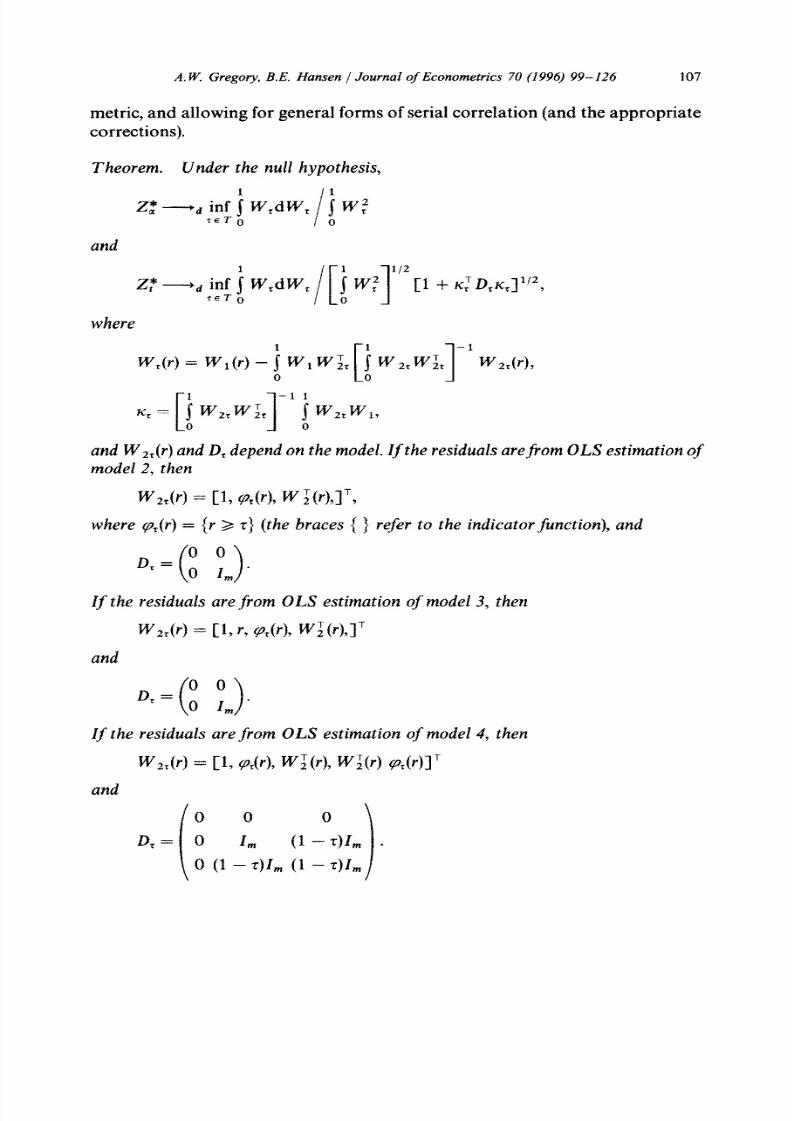
Theorem. Under the null hypothesis,

z,* ---+d inf j W,dW,rcl- 0

j Wf/ 0

and

2: -d inf i W,dW,reT0

where

and W ,,(r) and D, depend on the model. Z f the residuals arefrom OLS estimat ion of

model 2, then

W2,W = CL w?), W IOUT,

w here p&r) = (r 2 z f (the braces ( > refer to the indicator~nct ion), and

If t he residuals are from OLS estima tion of model 3, then

W 2,(rI = CL r, p&9, Wi(W

and

If t he residuals are from OLS estimat ion of model 4, then

W2,W = CL p&h W,‘(r),C(r) dr)l’

and




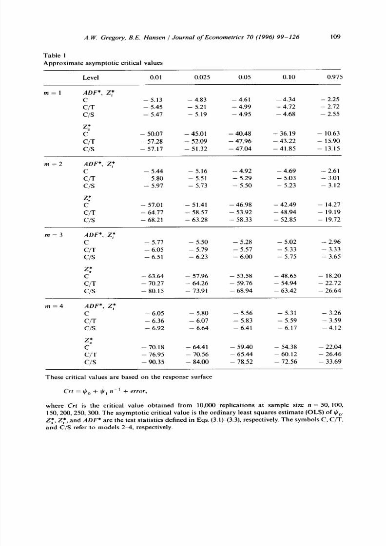
Calculating critical values

One standard way in which critical values have been obtained in situa-

tions where no closed-form expressions exist is to simulate a test statistic for a

large sample size for a large number of replications. In the present example, we

are unable to use large sample sizes since the recursive calculations which are

required over the sample are particularly time-consuming on even fast

computers. For instance, with n = 300 and 10,000 replications it took a

GATEWAY2000 486/33C over a week to do the relevant calculations for

the one regressor case (m = 1). To reduce the computational requirements we

adopt a procedure due to MacKinnon (1991). Using 10,000 replications for

each of the sample sizes n = 50, 100, 150,200,250, and 300 we obtain critical

values, Crt(n, p, m), where p is the percent quantile and m is the number of

regressors in the equation (excluding a constant and/or trend). We then estimate

by ordinary least squares for each p and m the response surface

Crt(n, p, m) = Ii/o + I i/In-1 + error.

Various other functional relations were tried (involving n-l”, L2, n-3’2) but

this one appeared to have the best fit (R2’s were generally over 0.98). The

asymptotic critical value is taken to be the OLS estimate 5,. While this

specification of the critical values seemed best overall, estimates of tiO changedon occasion by a factor of 2 under alternative specifications. Results for

p = 0.01,0.025,0.05,0.10, and 0.975 and m = 1,2,3,4 are presented in Table 1.

The symbols C, C/T, and C/S refer to breaks in the constant (C) and slope

coefficient (S) as defined in models 24.

5. A simple Monte Carlo experiment

In order to gauge the finite-sample properties of the proposed test, we conducta simple Monte Carlo experiment based upon the design of Granger and Engle

(1987) and also used in Banerjee, Dolado, Hendry, and Smith (1986). The model

in the absence of structural change is

yl, = 1 + 2 y2t + E,, st = PE,- 1 + St, S,- NID(0, l),

Yl, = Y2l + vt, rlt = Q-I + m,, o,-NID(O, I),

where yZt is scalar (m = 1). We first consider the size of the various tests with

p = 1, so that the null of no cointegration is true. In Table 2 we report the

rejection frequencies in 2500 replications at the 5% level of significance (we also

did 1% and lo%, and these are available upon request) using critical values

from Table 1. Two sample sizes (n = 50 and 100) are considered. Z,*, Z:, and

ADF* are the test statistics defined in Eqs. (3.1)-(3.3) respectively, and ADF is



A. W. Gregory. B.E. Hansen / Journal of Econometrics 70 (1996) 99-126

Table 1

Approximate asymptotic critical values

109

Level 0.01 0.025 0.05 0.10 0.975

m=l ADF*, Z:

C - 5.13 - 4.83 - 4.61 - 4.34 - 2.25

C/T - 5.45 - 5.21 - 4.99 - 4.72 - 2.12

CIS - 5.41 - 5.19 - 4.95 - 4.68 - 2.55

2:C - 50.07 - 45.01 - 40.48 - 36.19 - 10.63

C/T - 57.28 - 52.09 - 41.96 - 43.22 - 15.90

C/S - 57.17 - 51.32 - 47.04 - 41.85 - 13.15

m=2 ADF*, Z:

C - 5.44 - 5.16 - 4.92 - 4.69 - 2.61

C/T - 5.80 - 5.51 - 5.29 - 5.03 - 3.01

CIS - 5.91 - 5.13 - 5.50 - 5.23 - 3.12

2;C - 57.01 - 51.41 - 46.98 - 42.49 - 14.21

C/T - 64.77 - 58.57 - 53.92 - 48.94 - 19.19

CI S - 68.21 - 63.28 - 58.33 - 52.85 - 19.72

m=3 ADF*, Z:C - 5.71 - 5.50 - 5.28 - 5.02 - 2.96

C/ T - 6.05 - 5.19 - 5.57 - 5.33 - 3.33

CI S - 6.51 - 6.23 - 6.00 - 5.15 - 3.65

Z:C - 63.64 - 51.96 - 53.58 - 48.65 - 18.20

C/T - 70.27 - 64.26 - 59.76 - 54.94 - 22.12

c/s - 80.15 - 73.91 - 68.94 - 63.42 - 26.64

m=4 ADF*, Z:

C - 6.05 - 5.80 - 5.56 - 5.31 - 3.26

C/ T - 6.36 - 6.01 - 5.83 - 5.59 - 3.59

c / s - 6.92 - 6.64 - 6.41 - 6.17 - 4.12

Z:C - 70.18 - 64.41 - 59.40 - 54.38 - 22.04

C/T - 76.95 - 70.56 - 65.44 - 60.12 - 26.46

CIS - 90.35 - 84.00 - 78.52 - 12.56 - 33.69

These critical values are based on the response surface

where Crt is the critical value obtained from 10,000 replications at sample size n = 50, 100,

150,200,250,300. The asymptotic critical value is the ordinary least squares estimate (OLS) of $,.

Z:, Z:, and ADF* are the test statistics defined in Eqs. (3.13-(3.3), respectively. The symbols C, C/T.

and C/S refer to models 24, respectively.




the usual augmented Dickey-Fuller statistic (z = 1). The symbols C and C/T for

the usual ADF refer to regressions with a constant and a constant and a trend.

For ADF* and ADF the lag length K is selected on the basis of a t-test following

a procedure similar to Perron and Vogelsang (1992). We set K,,, to 6 and then

test downward (reducing K) until the last lag of the first difference included is

significant at the 5% level using normal critical values. Typically over all the

experiments including those with regime shifts, K was 0 or 1 but on occasion this

procedure led to lags of 6 being chosen.

From the size experiments (p = l), we see that the ADF*, Z:, and the

standard ADF tests are all biased away from the null. On the other hand, Z, is

biased towards the null, particularly at sample size n = 50. Also the size

distortion is larger for the ADF* compared to the standard ADF. In light of the

different size properties of the tests, in the remaining experiments where the

variables are cointegrated (with possible breaks), we calculate both nominal and

size-adjusted (in parentheses in the tables) power. The size adjustments are made

on the basis of the p = 1 results of Table 2.

Turning to power in the usual cointegration setting (model 1) we let p = 0 and

p = 0.5 (Table 2). With p = 0, the Z: and Z,* have highest size-adjusted power

with the standard ADF and the ADF* being roughly comparable and much

lower. Typically, the addition of the dummy variables lowered the lag length

chosen in these tests. Clearly from the perspective of power, faulty inclusion (i.e.,

including unnecessary regressors to capture breaks that do not exist) is not

a problem. As we would expect, all tests have lower power at sample size n = 50

when the error in the cointegrating regression is serially correlated (see Gregory,

1994). Interestingly with p = 0.5, the power (both nominal and size-adjusted) are

close for all the tests with the exception of the much smaller nominal power for

Z, at n = 50. There is also the tendency with more serial correlation for the

relative power decline to be larger at the smaller sample size for the structural

break tests for cointegration than the standard ADF tests.

We postulate a simple structural break for the intercept and then just the

slope (Table 3),

p, = pl, a, = a1 if t d [r n],

= p2, = tx2 if t > [r n],

E, = 0.5&,-i + s,,

YlI = Y2r + %? %=?t-l+w

The two errors LJt nd ot are uncorrelated and distributed as NID(O,l). Since in

applied work the errors are likely to be serially correlated, we make the break

experiments similar in structure to those in Table 2 with p = 0.5. A break point

occurs at z = 0.25, 0.5, and 0.75.



A. W . Gregory, B.E. Hansen /Journal of Econometrics 70 (1996) 99-126 111

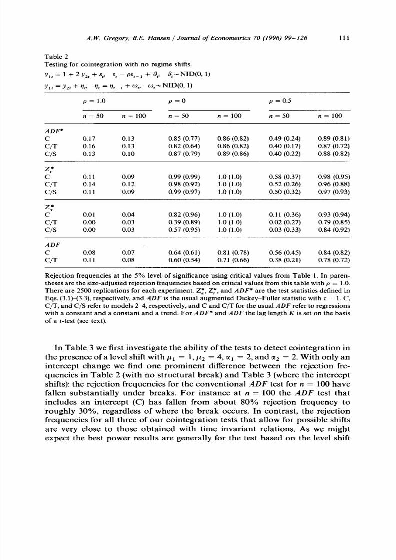
Table 2

Testing for cointegration with no regime shifts

~i,=l +~Y,,+E~, E,=P E,_~ +8,, 9,-NID(O,l)

~1, = ~2, + r/r> VI= nl-i + a,, w,-NID(0, )

p= 1.0 p=o p = 0.5

n = 50 n = 100 n = 50 n=lOO n = 50 n=lOO

ADF*

C 0.17 0.13 0.85 (0.77) 0.86 (0.82) 0.49 (0.24) 0.89 (0.81)

C/T 0.16 0.13 0.82 (0.64) 0.86 (0.82) 0.40 (0.17) 0.87 (0.72)

CP 0.13 0.10 0.87 (0.79) 0.89 (0.86) 0.40 (0.22) 0.88 (0.82)

=:C 0.11 0.09 0.99 (0.99) 1.0 (1.0) 0.58 (0.37) 0.98 (0.95)

C/T 0.14 0.12 0.98 (0.92) 1.0 (1.0) 0.52 (0.26) 0.96 (0.88)

CIS 0.11 0.09 0.99 (0.97) 1.0 (1.0) 0.50 (0.32) 0.97 (0.93)

=:C 0.01 0.04 0.82 (0.96) 1.0 (1.0) 0.11 (0.36) 0.93 (0.94)

C/T 0.00 0.03 0.39 (0.89) 1.0 (1.0) 0.02 (0.27) 0.79 (0.85)

CP 0.00 0.03 0.57 (0.95) 1.0 (1.0) 0.03 (0.33) 0.84 (0.92)

ADF

C 0.08 0.07 0.64 (0.61) 0.81 (0.78) 0.56 (0.45) 0.84 (0.82)

C/T 0.11 0.08 0.60 (0.54) 0.71 (0.66) 0.38 (0.21) 0.78 (0.72)

Rejection frequencies at the 5% level of significance using critical values from Table 1. In paren-

theses are the size-adjusted rejection frequencies based on critical values from this table with p = 1.0.

There are 2500 replications for each experiment. Zz, Z:, and ADF* are the test statistics defined in

Eqs. (3.1H3.3), respectively, and ADF is the usual augmented Dickey-Fuller statistic with r = 1. C,

C/T, and C/S refer to models 24, respectively, and C and C/T for the usual ADF refer to regressions

with a constant and a constant and a trend. For ADF* and ADF the lag length K is set on the basis

of a r-test (see text).

In Table 3 we first investigate the ability of the tests to detect cointegration in

the presence of a level shift with p1 = 1, p2 = 4, ctl = 2, and a2 = 2. With only an

intercept change we find one prominent difference between the rejection fre-

quencies in Table 2 (with no structural break) and Table 3 (where the intercept

shifts): the rejection frequencies for the conventional ADF test for n = 100 have

fallen substantially under breaks. For instance at n = 100 the ADF test that

includes an intercept (C) has fallen from about 80% rejection frequency to

roughly 30%, regardless of where the break occurs. In contrast, the rejection

frequencies for all three of our cointegration tests that allow for possible shifts

are very close to those obtained with time invariant relations. As we might

expect the best power results are generally for the test based on the level shift



T

e

3

S

u

ua

be

n

h

nec

a

so

a=

05

_

+

?

9

NID(01

Y

=

~

<+

v

V

=

~

+

QJ

o

NID(01

r

p=

p

=

a=

a=

p

=

1

pL=

1

f

=

2

a

=

n=

5

n

OO

n=

5

f=OO

02

05

07

02

05

07

02

05

07

02

05

07

A

F

C

04

01

04

02

05

02

CT

03

01

04

01

04

02

CS

03

01

03

01

03

02

2 &

0505

03

(02

0505

03

(02

0505

03

(03

CS

04

02

04

03

04

03

09

08

09

08

09

08

02

00

03

01

04

01

03

02

05

03

07

06

08

06

08

07

08

07

02

00

02

00

04

01

03

01

04

03

07

05

08

07

08

07

08

08

03

01

03

01

03

01

09

08

08

07

08

07

09

09

09

09

09

09

03

01

03

01

04

02

05

04

06

04

09

08

09

08

09

08

09

09

03

00

03

00

05

01

04

03

06

04

08

07

09

08

09

08

09

09

04

02

04

02

04

02

09

09

09

09

09

09

2C 01

03

01

03

01

03

09

09

09

09

09

09

00

01

00

00

03

04

08

08

CT

(02

(03

(03

(04

00

02

00

02

00

03

07

(08

07

08

08

08

00

01

00

01

00

02

02

02

03

CS

(04

06

07

00

03

00

03

00

03

07

(08

08

08

08

09

00

03

00

03

00

03

08

09

08

08

08

08

ADF

C

04

03

01

01

01

00

03

02

02

02

02

02

01

01

03

02

02

04

CT

03

(01

02

01

03

01

(05

(00

(00

(01

(02

(04

04

03

05

06

05

(01

01

00

01

00

03

01

01

01

02

02

05

05

R

e

o

e

e

a

h

5% e

o

sg

c

u

n

c

c

v

u

om T

e

1

n

2

e

c

o

n

p

e

h

ae

h

sz

a

u

e

ee

o

fe

e

b

o

c

c

v

u

om T

e

2wih

=

1O.S

T

e

2

o

dn

o

o

symb

s



A. W. Gregory, B.E. Hansen / Journal of Econometrics 70 (1996) 99-126 113

model 2 (C). Also power appears to be unaffected by the location of the break in

the sample.

In the same table we report results when the slope changes but the intercept is

fixed over the sample: pi = 1, p2 = 1, a1 = 2, and a2 = 4. As before the best

power results are obtained for those tests that allow for a shift in the slope (C/S).

Compared to the tests with no structural break (Table 2), the rejection frequen-

cies (both nominal and size-adjusted) for the (C) and (C/T) have fallen consider-

ably when z = 0.25 or 0.5. For this experiment, power rises as the breakpoint

occurs later in the sample. In a series of experiments we increased cr9relative to

(T,. As might be expected power falls as o9 rises relative to oo. Finally we note

that the standard ADF tests reject the null far less frequently compared to tests

which account for breaks especially if the slope break is in the earlier part of the

sample.

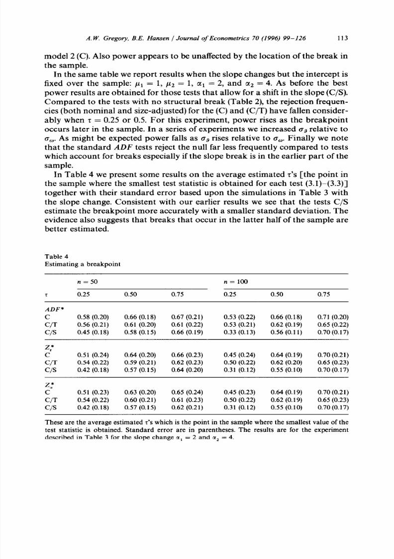
In Table 4 we present some results on the average estimated t’s [the point in

the sample where the smallest test statistic is obtained for each test (3.1)-(3.3)]

together with their standard error based upon the simulations in Table 3 with

the slope change. Consistent with our earlier results we see that the tests C/S

estimate the breakpoint more accurately with a smaller standard deviation. The

evidence also suggests that breaks that occur in the latter half of the sample are

better estimated.

Table 4

Estimating a breakpoint

n = 50 n=lOO

7 0.25 0.50 0.75 0.25 0.50 0.75

ADF*

C 0.58 (0.20) 0.66 (0.18) 0.67 (0.21) 0.53 (0.22) 0.66 (0.18) 0.71 (0.20)

C/T 0.56 (0.21) 0.61 (0.20) 0.61 (0.22) 0.53 (0.21) 0.62 (0.19) 0.65 (0.22)CIS 0.45 (0.18) 0.58 (0.15) 0.66 (0.19) 0.33 (0.13) 0.56 (0.11) 0.70 (0.17)

z:C 0.51 (0.24) 0.64 (0.20) 0.66 (0.23) 0.45 (0.24) 0.64 (0.19) 0.70 (0.21)

C/T 0.54 (0.22) 0.59 (0.21) 0.62 (0.23) 0.50 (0.22) 0.62 (0.20) 0.65 (0.23)

CIS 0.42 (0.18) 0.57 (0.15) 0.64 (0.20) 0.31 (0.12) 0.55 (0.10) 0.70 (0.17)

z:C 0.51 (0.23) 0.63 (0.20) 0.65 (0.24) 0.45 (0.23) 0.64 (0.19) 0.70 (0.21)

C/T 0.54 (0.22) 0.60 (0.2 1) 0.61 (0.23) 0.50 (0.22) 0.62 (0.19) 0.65 (0.23)

C/S 0.42 (0.18) 0.57 (0.15) 0.62 (0.21) 0.31 (0.12) 0.55 (0.10) 0.70 (0.17)

These are the average estimated 7’s which is the point in the sample where the smallest value of the

test statistic is obtained. Standard error are in parentheses. The results are for the experiment

described in Table 3 for the slope change OL,= 2 and a, = 4.



114 A. W. Gregory B.E. Hansen / Journal of Econometrics 70 (1996) 99-126

Overall the results with 2: appear to be the best in terms of size and power.

However, as we have seen this test is biased away from the null which can lead to

large gaps between nominal and size-adjusted power.

6. An illustrative example

The question of whether the long-run money-demand equation is stable has

received ample attention over the years. Two recent discussions are Lucas (1988)

and Stock and Watson (1993). As a practical example, we consider this question

in the context of our new tests using annual data (1901-1985) and quarterly data

(1960: l-1990:4). The long-run money-demand relation with no structural

breaks may be written as

ln(m,) - In@,) = fi + ~1~n(y,) + ff,r, + e,.

The annual data are from Lucas (1988) and m is Ml, p is the implicit price

deflator, y is the real net national product, and Y is the six-month commercial

paper rate. The quarterly data are from the CITIBASE tape; the series used are

GMPY, FXGM3, GMPY82, FMl, GNNP, GNNP82, and are seasonally

adjusted. This specification is identical to Lucas (1988) and Stock and Watson

(1991).

With this same data, Gregory, Nason, and Watt (1994) found that some of

Hansen’s (1992~) tests for structural breaks detected a break and that the

conventional ADF tests indicated that the null of no cointegration could be

rejected for the annual data but not for the quarterly. In Table 5 we report the

test statistics for our tests as well as the estimated breakpoint (in parentheses). In

addition, we calculate the test statistic for the conventional ADF test. For the

conventional ADF test the lag length for K (again selected on the basis of a t-test

as outlined in the Section 5) is 1 (annual) and 6 (quarterly) for both the C and

C/T tests. The lags selected for ADF* tests for the C, C/T, and C/S are (2,2,0) for

the annual and (0,0&i) or the quarterly data, respectively.

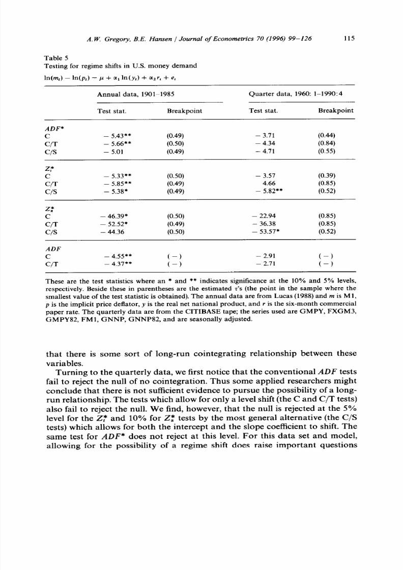
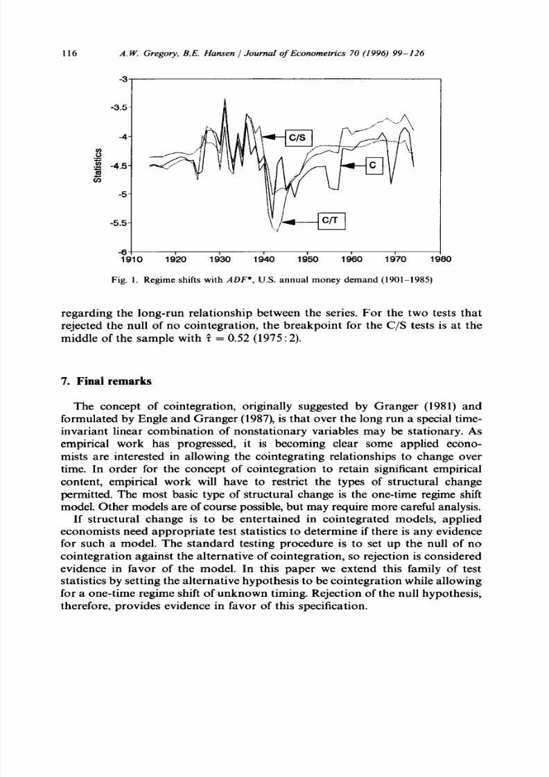
examining first the annual data, we find that the null hypothesis of no

cointegration is rejected (at the 5% level) by our new tests using the C and C/T

type formulations, but not using the C/S formulation. The smallest test statistic

occurred roughly at half of the sample (1944), and in Fig. 1 we graph the ADF(z)

using the annual data for C, C/T, and C/S over the truncated sample. Clearly

there is a well-defined single minimum for all three of these tests. Since the

conventional ADF test rejects the same null, it would be inappropriate to

conclude from this piece of information alone that there is a structural

break, since a conventional cointegrated system could produce this same

set of results. In fact, the point estimates for the second half of the sample (not

reported here) are economically meaningless, lending support to the view that

there is no structural break. On balance we believe that the evidence suggests



A. W. Gregory, B.E. Hansen 1 Journal of Econometrics 70 (1996) 99-126

Table 5

Testing for regime shifts in U.S. money demand

In(m) - ln(p,) = p + tll ln(y,) + azrt + e,

115

Annual data, 1901-1985 Quarter data, 1960: l-1990:4

Test stat. Breakpoint Test stat. Breakpoint

ADF*

C - 5.43** (0.49) - 3.71 (0.44)

C/T - 5.66** (0.50) - 4.34 (0.84)

CIS - 5.01 (0.49) - 4.71 (0.55)

z:C - 5.33** (0.50) - 3.57 (0.39)

C/T - 5.85** (0.49) - 4.66 (0.85)

CIS - 5.38: (0.49) - 5.82** (0.52)

-2C - 46.39* (0.50) - 22.94 (0.85)

C/T - 52.52* (0.49) - 36.38 (0.85)

CIS - 44.36 (0.50) - 53.57* (0.52)

ADF

C - 4.55** (-) - 2.91 (-)

C/T - 4.37** (-) - 2.71 (-)

These are the test statistics where an * and ** indicates significance at the 10% and 5% levels,

respectively. Beside these in parentheses are the estimated r’s (the point in the sample where the

smallest value of the test statistic is obtained). The annual data are from Lucas (1988) and m is Ml,

p is the implicit price deflator, y is the real net national product, and r is the six-month commercial

paper rate. The quarterly data are from the CITIBASE tape; the series used are GMPY, FXGM3,

GMPY82, FMl, GNNP, GNNP82, and are seasonally adjusted.

that there is some sort of long-run cointegrating relationship between these

variables.

Turning to the quarterly data, we first notice that the conventional ADF tests

fail to reject the null of no cointegration. Thus some applied researchers might

conclude that there is not sufficient evidence to pursue the possibility of a long-

run relationship. The tests which allow for only a level shift (the C and C/T tests)

also fail to reject the null. We find, however, that the null is rejected at the 5%

level for the Z: and 10% for Z,* tests by the most general alternative (the C/S

tests) which allows for both the intercept and the slope coefficient to shift. The

same test for ADF* does not reject at this level. For this data set and model,

allowing for the possibility of a regime shift does raise important questions



116 A. W. Gregory. B.E. Hansen 1 Journal of Econometrics 70 (1996) 99-126

‘I

-3.5-

r-l /\

-4-

8-

.g -4.5-(L1Ci

-5

-5.5-

-6 I1 9 1 0 1 9 2 0 1 9 3 0 1 9 4 0 1 9 5 0 1 9 6 0 1 9 7 0 l !

Fig. 1. Regime shifts with ADF*, U.S. annual money demand (1901-1985)

80

regarding the long-run relationship between the series. For the two tests that

rejected the null of no cointegration, the breakpoint for the C/S tests is at the

middle of the sample with ? = 0.52 (1975 :2).

7. Final remarks

The concept of cointegration, originally suggested by Granger (1981) and

formulated by Engle and Granger (1987), is that over the long run a special time-

invariant linear combination of nonstationary variables may be stationary. As

empirical work has progressed, it is becoming clear some applied econo-

mists are interested in allowing the cointegrating relationships to change over

time. In order for the concept of cointegration to retain significant empirical

content, empirical work will have to restrict the types of structural change

permitted. The most basic type of structural change is the one-time regime shift

model. Other models are of course possible, but may require more careful analysis.

If structural change is to be entertained in cointegrated models, applied

economists need appropriate test statistics to determine if there is any evidence

for such a model. The standard testing procedure is to set up the null of no

cointegration against the alternative of cointegration, so rejection is considered

evidence in favor of the model. In this paper we extend this family of test

statistics by setting the alternative hypothesis to be cointegration while allowing

for a one-time regime shift of unknown timing. Rejection of the null hypothesis,

therefore, provides evidence in favor of this specification.



A. W. Gregory, B.E. Hansen / Journal of Econometrics 70 (1996) 99-126 117

It is important to note, however, that this type of hypothesis test does not

provide much evidence concerning the question of whether or not there was

a regime shift, since the alternative hypothesis contains as a special case the

standard model of cointegration with no regime shift. The naive alternative of

examining the individual or joint significance of the dummy variables is danger-

ously flawed for two reasons. First, OLS estimation is not efficient, and test

statistics do not generally have asymptotic standard distributions under the

hypothesis of cointegration. Second, under the hypothesis of no regime shift, the

date of the break is not identified, so even efficient test statistics have non-

standard distributions. Appropriate statistics and their asymptotic distributions

for testing the hypothesis of no regime shift against the alternative of a regime

shift are given in Hansen (1992a) and Quintos and Phillips (1993). The test

statistics of the present paper complement these tests, and both types of test

statistics are potentially useful.

As illustrated in our analysis of the money-demand relationship in the

previous section, we believe that empirical investigations will be best served by

using a number of complementary statistical tests. One difficult task for the

applied researcher is to juggle these separate pieces of the puzzle, but we can

offer a few suggestions. The standard ADF statistic and our ADF* statistics both

test the null of no cointegration, so rejection by either statistic implies that there

is some long-run relationship in the data. If the standard ADF statistic does not

reject, but the ADF* does, this implies that structural change in the cointegrating

vector may be important. If both the ADF and the ADF* reject, no inference that

structural change has occurred is warranted from this piece of information alone,

since the ADF* statistic is powerful against conventional cointegration. In this

event, the tests of Hansen (1992a) are useful to determine whether the cointegrat-

ing relationship has been subject to a regime shift. Unfortunately at this stage we

have little guidance as to how to control for Type I error under such procedures

which suggests that additional Monte Carlo work would be worthwhile.

The analysis of this paper has been confined to the question of developing

residual-based tests for cointegration in the presence of a regime shift. We have

not addressed the issues of efficient testing or efficient estimation, and leave these

subjects for future research. For example, it would be interesting and useful to

develop an analogous set of test statistics using the likelihood ratio approach

advocated by Johansen (1988, 1991). Some progress along these lines has been

recently initiated by H. Hansen and Johansen (1993).

Appendix: P roof of the theorem

We will rigorously prove the Theorem for a simplified setting in which the test

statistic is constructed from residuals from the following regression model:

ylf = 4 yzt + 4 yztcptr + et, (A.l)




which is the same as model 4, except that there is no intercept or level shift. See

our working paper version, Gregory and Hansen (1992) for a complete proof for

model 4. To simplify the presentation we assume that y, = 0.

A. 1, Fundam ental convergence resul t s

Throughout the proof, * denotes weak convergence of the associated

probability measures with respect to the uniform metric over r E [O,l] or r E T,

where appropriate, and f-1 denotes the indicator function. Let S, = xi= 1 ai

be the cummulative sum of the innovations, and partition S, = (S,,, S,TJT in

conformity with u,. Set Sltr = Szt P,~ where ptr = {t > [nr] }, and set X,, =

(ST, S:,JT. It will be convenient to also define the subvector XZtr = (Si,, Si,)‘,as these are the regressors in our model (A.l).

The starting point for the asymptotic analysis is the multivariate invariance

principle

n - 1’2 f&] * B(z ), 64.2)

where B(z) is a vector Brownian motion with covariance matrix Q. This was

shown by Herrndorf (1984) (see Phillips and Durlauf, 1986, for the extension

to the vector case). Partition B(r) = (B, B:)T in confo~ity with St, define

B,,(r) = B,(r) q+(r) and X,(r) = (B(r)T, Btr(r)‘)’ where PJr) = (r >, z>, anddefine the subvector X,,(r) = (B2(r)T, B2,(r)T)T.

Our proof method involves explicitly writing out all test statistics as functions

of partial sums of functions of the data, in contrast to the proof method of Zivot

and Andrews (1992) who write the test statistics as explicit functions of the

indicator function &. Our method is more cumbersome notationally, but is

more convenient in terms of proving uniformity over the breakpoint r. The key

to our approach rests on the joint weak convergence of

(A-3)

-i BdBT + (1 - r)/t,f

(A-4)

where the weak convergence in (A.3) and (A.4) is with respect to the uniform

metric over r E [O, 11, and n = lim, (l/n) c:= 1E(S,u:+ i). (A.3) follows from (A.2)

and the continuous mapping theorem (CMT, see Billingsley, 1968, Thm. 5.1)

since si BBT is continuous with respect to r. (A.4) is proved under our assump-

tions by Hansen (1992b, Thm. 4.1). Note that the latter result is stronger than the

pointwise convergence theorems of Chan and Wei (1988) and Phillips (1988). To

ensure that there is no confusion with mere pointwise convergence, for the



A. W. Gregory, B.E. Hansen / Journal of Econometrics 70 (I 996) 99-126 119

remainder of the proof we will refer to results such as (A-3) and (A.4) as holding

‘uniformly over r’. The remainder of the proof is largely a series of repeated

applications of the CMT to (A.3), (A.4), and functions of these sample moments.

A.2 Least squares coeSficient process

(A.4) implies

(A.3

= dxrx:,

uniformly over r E [O,l).

Define kt = (a:, 6:) as the least-squares estimator of (A.1) for each z, and set

& = (1, - 62:)‘. It follows from (AS) and the CMT that

uniformIy over r E T. Note that we need to restrict z to a compact subset of (OJ)

since X2,, is multicolinear when r = 0 or r = 1.

A.3. Convergence to the stochastic integral process

Partition A and s2 in conformity with S,:

A=(;:: :::), 61=(;;; ;;;),



120 A. W. Gregory, B.E. Hansen / Journal qf Econometrics 70 (1996) 99-126

and set AZ. = (AZ1 Az2) and k2 = (LIT, n:JT. (AS) implies that

(A.7)

uniformly over r E [0, 11.

The process SZtr has differences

AS,,, = ASzt~7rr+ Sz,--lA%, (A4

where Ap t,, = plr - pt -lr = {t = [m ]}. Note that q+,Aq~~+~, = 0. To derive the

large-sample counterpart we need to define the differential dpI. Since pJr) is a step

function with a jump at r, dpr is naturally defined as the dirac function with the

property that for all functions f(.) with left-limits and ail a < z < 6,

lLfdpr = lim,,,f(z). Note that CJI~q+ = 0 since the left-limit of pz at t is 0. We then

define the differential d&,(r) = pro,(r) &(r) + B,(r) dq@), giving the relationships

; BdB;, = i BdB; + B(t)B2(r)T (A.9)0 r

and

i B,,dB:, = i B,,dB;.0 r

Using (A.@, (A.9), and (A.lO),

(A.lO)

LAS;,, Ir =

I

=+ (A.1 1)

i BdB: + (1 - t)k2 + B(r)B,(r)Tr

i B,dB; + (1 - s)&T I

=iX,dB:,+(l -r) ;,: ,

’[ 1



A. W. Gregory, 3.E. Hansen / Journal of Econometrics 70 (1996) 99-126 121

where the convergence is uniform over r E [0, 11. Setting dXJ = (dBT, dB:,)l,

then (A.7) and (A. 11) yield

t ,$ :,AX:+ ,r = ; ,iI X,J S:+ I 9 ; jl &A S:t+z)

=z. (A.12)

i X, dX: + A,,0

uniformly over r, where

n, = [

n (1 - +I.*

11 - $4.2 (1 - r)L& .A.4. Serial correlat ion coejk ient estim at e

Note that $, = ;l:X,, so by (A.2), (A.3), and the CMT,

* (A.13)

6 j. Xx-% = i x:*,

uniformli over r E 7’: where X,*(r) = B,(r) - (~~B,X ~,)(j~ X2rX~r)-‘X2,(r) is

the stochastic process in (r,z) obtained by projecting B,(r) orthogonal to X,,(r).

Define c = [fill - Q1251;~G&J112, and set W ,(r) = opl[B1 - G?1252;~B2(r)J

and W ,(r) = SL1,;“*B,fr), so that Wr 5 BM(1) is independent of W2 = BM(Z,).

By standard projection arguments, X:(r) = oW ,(r), where W ,(r) = W ,(r) -

(S~W ,WI,)(f~W ,,W :,)-’ W2,( ), and W,,(r) = [W:(r), W;(r) pJr)]‘. Thus

(A. 13) becomes

uniformly over r E T.

Similarly using (A.12) and the CMT,

”

(A. 14)

(A.15)

qr’ J!,dX: + A, yl, = o* 3 W , d W , + q: A ,tjt ,0 > 0



122 A.W. Gregory B.E. Hansen / Journal of Econometrics 70 (1996) 99-126

uniformly over z E T. (A.14) (A.13, and the CMT yield

uniformly over 7.~ T. The limit in (A.16) exists for T E T since 1: W,’ > 0 as. by

Lemma A.2 of Phillips and Hansen (1990).

A.5. Bias correction

The Phillips’ statistics are constructed using the statistic 2, = cy=l w(j/M)

x (l/n) 1, tt_izGrt where ir,, = SC,, fi$_ Ir = d& - (jr - l)e*,_ Ir. For brevity,

denote w(j/M) by Wj. Now by the triangle inequality and Holder’s inequality,

uniformly in z, since MI,,& --t 0 and sup, In(/?, - 1)I = O,( 1) by (A-16). Sim-

ilarly, we can replace d&,-jr with ir_jr to show that

uniformly in T. Now note that

(A-17)

(A-18)

In Hansen (1992c, Thm. 1), it was shown under our assumptions that

f wji _i Ut-jU:+pA,j=l I-l+j



A. W. Gregory, B.E. Hansen 1 Journal of Econometrics 70 (1996) 99-126 123

which gives the asymptotic behavior of the upper-left element of (A.18). A slight

modification of the proof in Hansen (1992~) yields the stronger result

jt, wjt,:?+jt-jU:+pTA, (A. 19)

uniformly in z E [0, 11. This is possible since Theorem 1 in Hansen (1992~) is

based on a moment inequality which can be strengthened to a maximal inequal-

ity via Lemma 2 of Hansen (1991).

Now using (A.8) we can obtain the asymptotic behavior of the lower-left

element of (A.18):

=j$lw.iiM

UZt-jrU: + C Wj'St 3 [ n r l + j j=l

n Z[nr]- l"&]+j

+,(I - w2,

uniformly in r E [0, l] by (A.19) and the fact that

(A.20)

where the final inequality follows from Markov’s inequality and

"?I:: ii.:

2

wj"t+j = O(l),

3-l

which is an application of Corollary 3 of Hansen (1991).Similar analysis for the upper-right and lower-right elements of (A.18), com-

bined with (A.19) and (A.20), yield the complete result

(A.21)

uniformly in r E [0, 11. Finally, (A.17) (A.21), the fact that A& = $4X,,, and

(A.3) yield

M

Jr=?: C Wj~~AXt-jrAXL$r + op(l)*~:A~r,j=l t

uniformly over z E T.

(A.22)



124 A. W. Gregoty, B.E. Hansen 1 Journal of Econometrics 70 (1996) 99-126

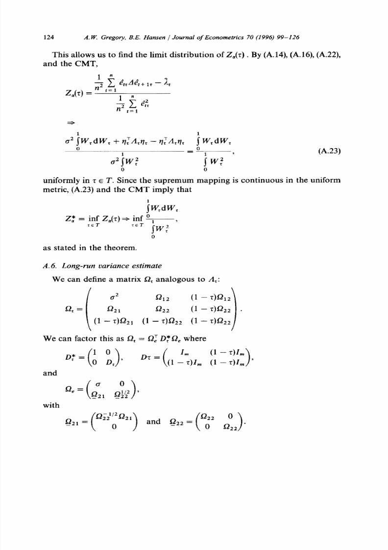
This allows us to find the limit distribution of Z,(z) . By (A.14), (A.16), (A.22),

and the CMT,

g2 jW,dW, + r:&ul, - $41, j- W,dW,0 0

rizjW,z

=

iw: ’

(A.23)

0

uniformly in 7 E T. Since the supremum mapping is continuous in the uniform

metric, (A.23) and the CMT imply that

jW,dW,

2: = inf Z,(z) * inf +----,ZET

reT iw:

as stated in the theorem.

A. 6. Long-run variance estimate

We can define a matrix L&analogous to A,:

O2 5212

52, =

i

a21 sz

(1 -z)& (1 - :;Q22

We can factor this as 4 = St,’Dyf2, where

and

with



A.W.Gregory, B.E. Hansen /Journal of Econometrics 70 (1996) 99-126

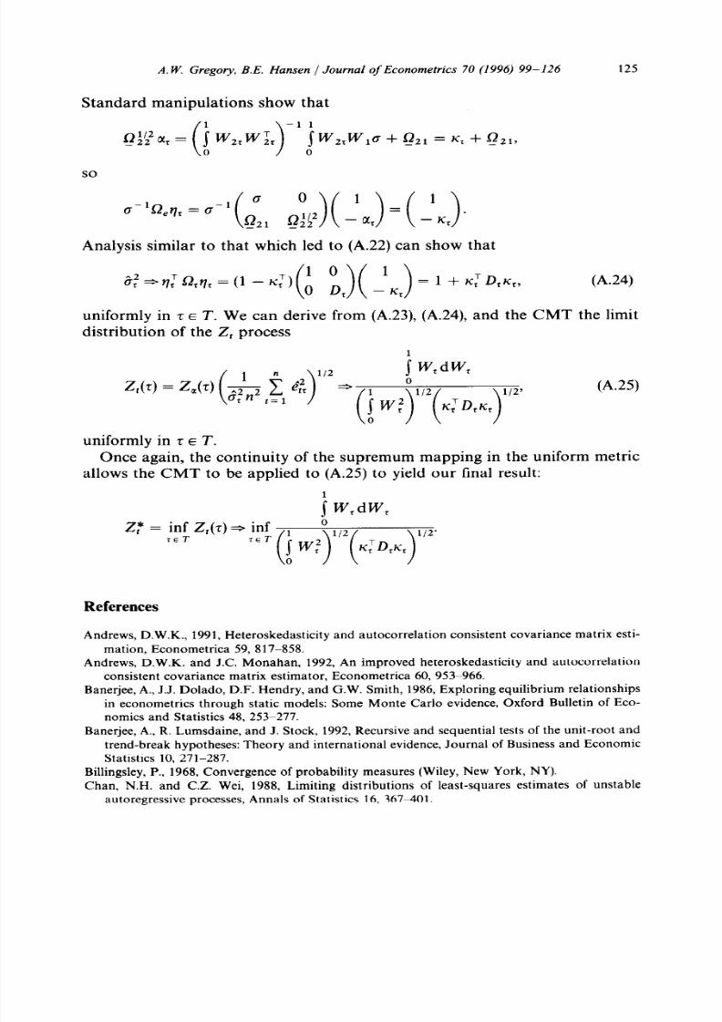
Standard manipulations show that

SO

a-‘Q,& = 0-l (Ll !‘)(l4) -‘G)’Analysis similar to that which led to (A.22) can show that

125

uniformly in z E T. We can derive from (A.23), (A.24), and the CMT the limit

distribution of the Z, process

(A.25)

uniformly in r E T.Once again, the continuity of the supremum mapping in the uniform metric

allows the CMT to be applied to (A.29 to yield our final result:

z: = nf x7) );f (i wijl,2(K;D.Kr)1,2.TET

References

Andrews, D.W.K., 1991, Heteroskedasticity and autocorrelation consistent covariance matrix esti-

mation, Econometrica 59, 817-858.

Andrews, D.W.K. and J.C. Monahan, 1992, An improved heteroskedasticity and autocorrelation

consistent covariance matrix estimator, Econometrica 60, 953-966.

Banerjee, A., J.J. Dolado, D.F. Hendry, and G.W. Smith, 1986, Exploring equilibrium relationships

in econometrics through static models: Some Monte Carlo evidence, Oxford Bulletin of Eco-

nomics and Statistics 48, 2533277.

Banerjee, A., R. Lumsdaine, and J. Stock, 1992, Recursive and sequential tests of the unit-root and

trend-break hypotheses: Theory and international evidence, Journal of Business and Economic

Statistics 10, 271-287.

Billingsley, P., 1968, Convergence of probability measures (Wiley, New York, NY).

Chan, N.H. and C.Z. Wei, 1988, Limiting distributions of least-squares estimates of unstable

autoregressive processes, Annals of Statistics 16, 367401.



126 A. W. Gregory, B.E. Hansen 1 Journal of Econometrics 70 (1996) 99-126

Christiano, L.J., 1992, Searching for a break in GNP, Journal of Business and Economic Statistics

10, 237-250.

Engle, R.F. and C.W.J. &anger, 1987, Cointegration and error correction: Representation, estima-

tion, and testing, Econometrica 55, 251-276.&anger, C.W.J., 1981, Some properties of time series data and their use in econometric model

specification, Journal of Econometrics, 121-130.

Gregory, A.W., 1994, Testing for cointegration in linear quadratic models, Journal of Business and

Economic Statistics 2, 347-360.

Gregory, A.W., J.M. Nason, and D. Watt, 1994, Testing for structural breaks in cointegrated

relationships, Journal of Econometrics, forthcoming.

Hansen, B.E., 1991, Strong laws for dependent heterogeneous processes, Econometric Theory 7,

213-221.

Hansen, B.E., 1992a, Tests for parameter instability in regressions with I( 1) processes, Journal of

Business and Economic Statistics 10, 321-335.

Hansen, B.E., 1992b, Convergence to stochastic integrals for dependent heterogeneous processes,Econometric Theory 8,489-500.

Hansen, B.E., 1992c, Consistent covariance matrix estimation for dependent heterogeneous pro-

cesses, Econometrica 60, 967-972.

Hansen, H. and S. Johansen, 1993, Recursive estimation in cointegrated VAR models, Unpublished

manuscript (University of Copenhagen, Copenhagen).

Herrndorf, N., 1984, A functional central limit theorem for weakly dependent sequences of random

variables, Annals of Probability 12, 829-839.

Johansen, S., 1988, Statistical analysis of cointegrating vectors, Journal of Economic Dynamics and

Control 12, 231-254.

Johansen, S., 1991, Estimation and hypothesis testing of cointegration vectors in the presence of

linear trend, Econometrica 59, 1551-1580.

Lucas, R.E., 1988, Money demand in the United States: A quantitative review, Carnegie-Rochester

Conference Series on Public Policy 29, 137-168.

MacKinnon, J.G., 1991, Critical values for cointegration tests, in: R.F. Engle and C.W.J. Granger,

eds., Long-run economic relationships: Readings in cointegration (Oxford Press, Oxford)

267-276.

Perron, P., 1989, The great crash, the oil price shock, and the unit root hypothesis, Econometrica 57,

1361-1401.

Perron, P. and T.J. Vogelsang, 1992, Nonstationarity and level shifts with an application to

purchasing power parity, Journal of Business and Economic Statistics 10, 301-320.

Phillips, P.C.B., 1987, Time series regression with a unit root, Econometrica, 55, 277-301.

Phillips, P.C.B., 1988, Weak convergence of sample covariance matrices to stochastic integrals via

martingale approximations, Econometric Theory 4, 528-533.

Phillips, P.C.B. and S.N. Durlauf, 1986, Multiple time series regression with integrated processes,

Review of Economic Studies 53,4733495.

Phillips, P.C.B. and B.E. Hansen, 1990, Statistical inference in instrumental variables regression with

I(1) processes, Review of Economic Studies 57, 99-125.

Phillips, P.C.B. and S. Ouliaris, 1990, Asymptotic properties of residual based tests for cointegration,

Econometrica, 58, 165-193.

Quintos, C.E. and P.C.B. Phillips, 1993, Parameter constancy in cointegrating regressions, Empiri-

cal Economics 18, 675-703.

Stock, J.H. and M.W. Watson, 1993, A simple estimator of cointegrating vectors in higher orderintegrated systems, Econometrica 61, 783-820.

Zivot, E. and D.W.K. Andrews, 1992, Further evidence on the great crash, the oil-price shock, and

the unit-root hypothesis, Journal of Business and Economic Statistics 10, 251-270.

cointegration article

Documents