colala: the computation and language lab at uc berkeley

Psychological ReviewThe Logical Primitives of Thought: Empirical Foundationsfor Compositional Cognitive ModelsSteven T. Piantadosi, Joshua B. Tenenbaum, and Noah D. Goodman

Online First Publication, April 14, 2016. http://dx.doi.org/10.1037/a0039980

CITATION

Piantadosi, S. T., Tenenbaum, J. B., & Goodman, N. D. (2016, April 14). The Logical Primitives ofThought: Empirical Foundations for Compositional Cognitive Models. Psychological Review.Advance online publication. http://dx.doi.org/10.1037/a0039980

The Logical Primitives of Thought: Empirical Foundations forCompositional Cognitive Models

Steven T. PiantadosiUniversity of Rochester

Joshua B. TenenbaumMassachusetts Institute of Technology

Noah D. GoodmanStanford University

The notion of a compositional language of thought (LOT) has been central in computational accounts ofcognition from earliest attempts (Boole, 1854; Fodor, 1975) to the present day (Feldman, 2000; Penn,Holyoak, & Povinelli, 2008; Fodor, 2008; Kemp, 2012; Goodman, Tenenbaum, & Gerstenberg, 2015).Recent modeling work shows how statistical inferences over compositionally structured hypothesisspaces might explain learning and development across a variety of domains. However, the primitivecomponents of such representations are typically assumed a priori by modelers and theoreticians ratherthan determined empirically. We show how different sets of LOT primitives, embedded in a psycho-logically realistic approximate Bayesian inference framework, systematically predict distinct learningcurves in rule-based concept learning experiments. We use this feature of LOT models to design a set oflarge-scale concept learning experiments that can determine the most likely primitives for psychologicalconcepts involving Boolean connectives and quantification. Subjects’ inferences are most consistent witha rich (nonminimal) set of Boolean operations, including first-order, but not second-order, quantification.Our results more generally show how specific LOT theories can be distinguished empirically.

Keywords: language of thought, concept learning, Bayesian modeling

One of the most powerful features of human cognition is ourability to create, manipulate and communicate novel structuredideas—concepts such as prime number, half-sister, the tallestbuilding in Cambridge, most, or most but not all. Such conceptsare interesting to cognitive psychologists because they are at theheart of how we humans think flexibly and productively, extendingour thinking into novel situations, tasks, and domains. They are

also central to how we produce and comprehend language. From acomputational viewpoint, these concepts are interesting in partbecause they can be characterized using logical machinery: sketch-ing informally, the Green Building is the tallest building in Cam-bridge if for all other buildings b, the Green Building is taller thanb; two girls are half-sisters if there exists exactly one parent thatthey share; most As are Bs if (according to one standard account)the cardinality of the subset of As that are Bs is larger than thesubset of As that are not Bs (Montague, 1973). Human fluencywith such concepts likely reflects deep computational properties ofboth thinking and language, suggesting to many theorists (Hahn &Chater, 1998; Gentner, 1983; Penn, Holyoak, & Povinelli, 2008;Kemp, 2012; Goodman, Tenenbaum, & Gerstenberg, 2015) waysin which conceptual systems cannot be limited to stored examplesand prototypes, but in some form must incorporate rule-like rep-resentations that are defined in terms of abstract operations andthat compose flexibly to create new such representations.

Different branches of cognitive science have developed com-plementary approaches to study compositionally in humanthought. For example, in linguistics, formal semantics has soughtto characterize the logical structure necessary to capture referencefor theoretically interesting fragments of natural language, oftenwith a focus on quantifiers such as some, all, and most (Montague,1973). In artificial intelligence, researchers have developedgeneral-purpose architectures for human-like knowledge represen-tation and reasoning based on predicate logic, often first-orderlogic but also using higher-order logics such as the lambda calcu-lus, and often integrated with probability to support reasoningunder uncertainty, inductive learning and abductive inference

Steven T. Piantadosi, Department of Brain and Cognitive Sciences,University of Rochester; Joshua B. Tenenbaum, Department of Brain andCognitive Sciences, Massachusetts Institute of Technology; Noah D.Goodman, Department of Psychology, Stanford University.

This work was supported by an NSF Graduate Research Fellowship (toSteven T. Piantadosi) and a S.B.E. Dissertation Award in Linguistics (toSteven T. Piantadosi). This work was also supported by the Eunice KennedyShriver National Institute of Child Health & Human Development of theNational Institutes of Health under Award F32HD070544. The content issolely the responsibility of the authors and does not necessarily represent theofficial views of the National Institutes of Health. We are extremely gratefulto Roger Shepard, Jesse Snedeker, Susan Carey, Roman Feiman, EvelinaFedorenko, Ted Gibson, and Leon Bergen for insightful and constructiveconversations at various stages of this work. Data and code for this paper areavailable at http://colala.bcs.rochester.edu/data/PiantadosiTenenbaumGoodmanPsychReview.

Correspondence concerning this article should be addressed to Steven T.Piantadosi, Department of Brain and Cognitive Sciences, University ofRochester; 358 Meliora Hall, Box 270268, Rochester, NY 14627-0268.E-mail: [email protected]

Thi

sdo

cum

ent

isco

pyri

ghte

dby

the

Am

eric

anPs

ycho

logi

cal

Ass

ocia

tion

oron

eof

itsal

lied

publ

ishe

rs.

Thi

sar

ticle

isin

tend

edso

lely

for

the

pers

onal

use

ofth

ein

divi

dual

user

and

isno

tto

bedi

ssem

inat

edbr

oadl

y.

Psychological Review © 2016 American Psychological Association2016, Vol. 123, No. 2, 000 0033-295X/16/$12.00 http://dx.doi.org/10.1037/a0039980

1

(Levesque, Pirri, & Reiter, 1998; Muggleton & De Raedt, 1994;Milch, Marthi, & Russell, 2004; Russell & Norvig, 2009; Domin-gos & Richardson, 2007; Richardson & Domingos, 2006; Good-man, Mansinghka, Roy, Bonawitz, & Tenenbaum, 2008; Shapiro,Pagnucco, Lespérance, & Levesque, 2011). In cognitive psychol-ogy, the classic empirical method for studying compositionalthought has used concept learning experiments, where participantslearn various rule-based concepts from examples, and the rules aremost naturally represented as simple or more complex functions oflogical primitives (e.g., Bruner, Goodnow, & Austin, 1956;Shepard, Hovland, & Jenkins, 1961). By studying characteristicpatterns of mistakes learners make, and which concepts are harderor easier to learn, researchers aim to discover something about theprimitives and means of combination in human symbolic thought.

Our work here builds most directly on this cognitive psychologytradition of studying rule-based concept learning, but integrates ele-ments of the formal semantics and AI traditions, along with newmethods for computational cognitive modeling and web-based exper-imentation. This allows us to study the building blocks of composi-tional thought on a previously unprecedented scale, and to ask ques-tions that have not previously been amenable to empirical inquiry.Specifically, we make three main contributions. We study empiricallythe dynamics of how people induce a much broader space of rulesthan previous work has examined, including over 100 distinct con-cepts varying significantly in complexity and logical structure. Wealso show that people’s probabilistic generalization behavior in thesetasks can be quantitatively well described by a memory-constrainedBayesian learning model. Finally, and most importantly, we showhow the basic building blocks of the model’s compositional hypoth-esis space can be inferred from the large-scale patterns of participants’responses. This yields insight into the primitive representations andoperations in the combinatorial language of thought that people bringto this task, and presumably other settings of symbolic thinking andreasoning.

We build on recently developed computational tools and empir-ical techniques that have allowed detailed modeling of how peoplelearn symbolically structured concepts across a variety of domains(e.g., Nosofsky, Palmeri, & McKinley, 1994; Kemp, Goodman, &Tenenbaum, 2008a; Kemp, 2009; Piantadosi, 2011; Kemp, 2012;Ullman et al., 2012). This work formalizes learning as some kindof rational inductive inference over a compositional representationsystem, or language of thought (LOT; Fodor, 1975; Boole, 1854).For instance, learning models might posit that people initially haveaccess to simple logical operations (e.g., and, or, and not), quan-tifiers (like forall and exists), or computational primitives (e.g.,�-abstraction or combinators). The task of learners is then tocompose these primitives into a rule denoting a concept that fitsthe observed examples in some approximately optimal way, asmeasured by posterior probability in a Bayesian framework orencoding length in an information-theoretic framework. Morebroadly, beyond their ability to describe how people learn rule-based concepts in specific laboratory tasks, models of this sort aretheoretically appealing as a complement to other frameworks formodeling human learning such as connectionism, because of theirability to explain how inductive learning integrates with compo-sitionality, productivity and other core features of symbolic cog-nition (Fodor & Pylyshyn, 1988; Fodor, 2008; Tenenbaum, Kemp,Griffiths, & Goodman, 2011; Goodman, Tenenbaum, Feldman, &Griffiths, 2008).

In a prototypical example of this approach, Goodman et al. (2008)presented a rational analysis of rule-based concept learning based onBayesian induction of the Boolean expressions (built from connec-tives like and, or, and not) most likely to have generated the observedexample labels for a concept, and showed how this could explain bothclassic results in the literature and graded patterns of generalization innew experiments with higher-dimensional feature spaces. Their ap-proach has been extended to learning richer logical theories (Kemp etal. 2008a; Kemp, 2012), as well as conceptual domains like magne-tism (Ullman et al., 2012), semantic hierarchies (Katz, Goodman,Kersting, Kemp, & Tenenbaum, 2008), number concepts (Piantadosi,Tenenbaum, & Goodman, 2012), and function words (Piantadosi,Goodman, & Tenenbaum, 2014). Kemp (2012) provides an exhaus-tive characterization of logical domains such models can be formu-lated over (a “conceptual universe”) and shows that a rule inferencescheme based on minimal description length—closely related to theBayesian posterior probability—provides a compelling quantitative fitto behavioral data across a wide range of conceptual domains.

In these and most other prior efforts, the components and rulesof combination, which together characterize a representation sys-tem, have been assumed a priori with the analysis focused ondemonstrating the in-principle viability of compositional, LOT-style learning. For instance, Goodman, Tenenbaum et al. (2008)assumed that learners form compositions in disjunctive normalform (disjunctions of conjunctions of primitives). This assumptionamounts to a psychological hypothesis about the format of con-ceptual representations: it assumes that learners construct Booleanrules as disjunctions of conjunctions of features—as opposed to, forinstance, conjunctions of disjunctions, horn clauses, or free combina-tion of logical operations. Beyond the rules of combination, suchtheories also formalize a set of primitives, functions that are assumedto be available before the process of compositional hypothesis for-mation begins. It is natural to think of these primitives as the innateconceptual representations that learners use to build complex con-cepts. However, the effective set of primitives may also include onesdefined using the innate set, and thus include operations that havebeen learned at an earlier age. As we study adults, the primitives canbe seen as the key operations that are available to our subjects inunderstanding new logical concepts.

In the case of Boolean concept learning, there are many logi-cally possible sets of primitives that have been used across differ-ent domains of cognitive science, AI, and machine learning. In oneextreme, all Boolean functions can be constructed from one singleprimitive such as NAND (not-and, also known as the “Shefferstroke”). In the other extreme, Boolean concepts might psycho-logically depend on a rich set of redundant primitives, includingoperations like conjunction, disjunction, negation, implication, andso forth as are used in modern computer architectures. The prob-lem of the underdetermination of representational primitives isfaced even more broadly for systems that extend beyond Booleanconcepts: there are many possible primitives that would permitTuring-complete computational concepts. A coarse characteriza-tion of the right system can be made in terms of computationalpower: representations must be capable of supporting the knowl-edge people have and the computations they perform (Marr, 1982).For instance, human representational systems must extend beyondsimple Boolean propositional logic since such systems that lackquantification provably cannot express concepts like tallest. How-ever, descriptions based only on computational power are always

Thi

sdo

cum

ent

isco

pyri

ghte

dby

the

Am

eric

anPs

ycho

logi

cal

Ass

ocia

tion

oron

eof

itsal

lied

publ

ishe

rs.

Thi

sar

ticle

isin

tend

edso

lely

for

the

pers

onal

use

ofth

ein

divi

dual

user

and

isno

tto

bedi

ssem

inat

edbr

oadl

y.

2 PIANTADOSI, TENENBAUM, AND GOODMAN

underdetermined. As the Boolean case illustrates, two representa-tions can be equally expressive—capable of solving the samecomputational problems—yet distinct in how they achieve thatcomputational power (see, e.g., Hackl, 2009; Pietroski, Lidz,Hunter, & Halberda, 2009, for examples in semantics). Any po-tential set of primitives and rules for combination can be regardedas a scientific hypothesis about how compositional concepts mayarise in mind—a hypothesis that a mature LOT framework shouldseek to evaluate empirically.

Here we present a formal modeling approach that aims to discoverwhich particular LOT features—which primitives and rules of com-bination—provide the best account of how people learn and reason ina given domain of compositional thought. Our approach cruciallyexploits the classic insight that representational simplicity is a majordeterminant of learnability, with learners preferring to infer rules thatare concise in their representational system (Neisser & Weene, 1962;Haygood, 1963; Feldman, 2000, 2003c, 2003b; Chater & Vitányi,2003; Goodman, Tenenbaum et al., 2008; Kemp et al. 2008a; Kemp,2012). Analogously in modeling, simplicity plays a key role in modelselection because simple models are more parsimonious (e.g., Conk-lin & Witten, 1994), explaining the data with fewer free parameters orarbitrary stipulations. This property makes a simplicity bias a sensiblepsychological strategy.

The existence of a human bias for representational simplicityallows us to potentially reverse engineer likely components of theLOT since different hypothesized LOTs will measure simplicity indifferent ways. As a result, they make different empirical predic-tions about what generalizations participants should make fromdata and what concepts should be easy to learn (e.g., what conceptsare “simple”). A key example for our purposes is Feldman (2000),who showed that difficulty with learning Boolean concepts iswell-modeled by the concept’s description length in logic. Forexample, participants would find it harder to learn the exclusivedisjunction (XOR),

[red AND [NOT square]] OR [[NOT red] AND square]

(1)

than the nonexclusive disjunction

red OR square (2)

since the former has a longer description in standard Booleanlogic, requiring more primitive logical connectives.

However, as is often pointed out in philosophical discussions ofinduction (Goodman, 1955), what counts as “simple” is not purelyobjective. For instance if people’s representational system in-cluded the exclusive-or function (XOR) as a primitive, then thecomplexity—and therefore learning difficulty—for the above twoconcepts would be equal. Concept 2 could be expressed the sameway, but Concept 1 becomes

red XOR square (3)

which uses only a single logical operation. This only emphasizesa version of Goodman’s Grue problem: Concept 1 is not morecomplex than Concept 2 in any independent, objective sense.1

This philosophical puzzle is also an experimental tool: if par-ticipants do find Concept 2 easier than Concept 1, that providesevidence that human cognition measures simplicity via a LOT inwhich XOR is not primitive. Here, we take this simple idea and

implement it in a large-scale computational and experimentalstudy examining a wide range of concepts with state-of-the-artlearning and data analysis tools. Building on Kemp (2009, 2012),and motivated by both classic work in formal semantics (Mon-tague, 1973), AI (Levesque et al., 1998; Muggleton & De Raedt,1994; Milch et al., 2004; Russell & Norvig, 2009; Domingos &Richardson, 2007; Richardson & Domingos, 2006; Goodman,Mansinghka, et al. 2008; Shapiro et al., 2011), and more recentcognitive accounts of symbolic thinking (Gentner, 1983; Penn etal., 2008), our study moves beyond simple Boolean concepts andalso examines those involving quantification and relational terms.

The outline of this paper is as follows. In the next section, wepresent a large-scale concept learning experiment that taught par-ticipants Boolean and quantificational concepts. We then describehow we formalize the LOT in terms of �-calculus, and then presenttwo coordinated models. First, we develop a learning model that—like participants in the study—takes observed data and infers likelyLOT expressions. As we show, the learning model is capable ofinferring quite complex concepts from data, and the generaliza-tions it makes closely track those of participants. Then, we presenta data analysis model that uses participants’ experimental data toinfer unknown parameters of the learning model including theprobability of different primitives and participants’ memory-decayparameters. The details of these models are provided in the Ap-pendices, and we focus in the main text on intuitively describingtheir key properties. Our primary analysis is a model-based com-parison that quantifies the fit of different LOTs to human learningpatterns. We first apply these methods to only Boolean concepts inthe experiment, and then to concepts involving quantification. Ourresults provide quantitative evidence against intuitively implausi-ble logical bases, evidence for compositional logical rules with arich set of logical connectives that include first- but not second-order quantification. Most importantly, our method shows howdistinct LOTs can be firmly grounded as empirically testablescientific theories.

Before moving into the body of the paper, we should delimit ourgoals in several ways to avoid potential misunderstandings. Al-though our focus is on symbolic thinking, and the logical structureof the “language of thought” that underlies it, we do not mean toimply that all or even most human thinking is of this form. Quitethe contrary: we grant that much of how people think about theworld draws on other kinds of representations, such as perceptuallygrounded simulations (Battaglia, Hamrick, & Tenenbaum, 2013)or probabilistic expectations (Griffiths & Tenenbaum, 2006). Like-wise, although we focus on a certain class of concept learning taskswith concepts defined by logical rules, we do not mean to suggestthat all or even most human concepts take this form. Manyconcepts, especially those for basic-level natural kind categories,may be best thought of in other ways (Rosch & Mervis, 1975;Medin & Smith, 1984; Medin, 1989; Medin & Ortony, 1989;Hampton, 1998; Murphy, 2002; Hampton, 2006). Different cate-gorization tasks may even rely on distinct systems and processes(Ashby & Maddox, 2005).

1 Tools like Kolmogorov complexity (Li & Vitányi, 2008) come close toresolving this problem, providing a complexity metric that is arbitrary onlyup to an additive constant.

Thi

sdo

cum

ent

isco

pyri

ghte

dby

the

Am

eric

anPs

ycho

logi

cal

Ass

ocia

tion

oron

eof

itsal

lied

publ

ishe

rs.

Thi

sar

ticle

isin

tend

edso

lely

for

the

pers

onal

use

ofth

ein

divi

dual

user

and

isno

tto

bedi

ssem

inat

edbr

oadl

y.

3LOGICAL PRIMITIVES OF THOUGHT

However, we do think that logically structured concepts havesometimes been unfairly maligned as “unnatural”. The evidencefor a rich ability to process logical concepts can be seen in manydomains (e.g., Tenenbaum et al., 2011), including number andmathematics, social systems, taxonomies, and complex causalprocesses. The need for structured concepts becomes even moreevident in natural language, where languages contain words toexpress a variety of logical relations, whose meanings are typicallycaptured in formal theory only in with structured, logical systems.To illustrate in English, these words include quantifiers (e.g.,every) and other determiners (e.g., the), conjunctions (e.g., and),kinship terms (e.g., great uncle), prepositions (in), and markers ofdiscourse relations (e.g., because) expressing relations betweenclauses. Below the level of words, morphemes like –est combinewith words to form superlatives whose meaning is most naturallycaptured with logic: someone is the “tallest” if their height isgreater than everyone else, a sublexical concept involving first-order quantification. The full power of abstract logical structurecan be seen in the compositional phrases formed in natural lan-guage—phrases like “the tallest building in Cambridge” combinesimpler, constituent meanings into complex logical structures thatare able to communicate a huge variety of meanings. There islogical structure in language even above the level of sentences,including in the discourse relations between sentences (Wolf &Gibson, 2005) and in recursive patterns of dialogue and pragmatics(Levinson, 2013). Our goal here is not to account for the full set ofphenomena that cognitive psychologists have been interested inunder the banner of “concepts” (Margolis & Laurence, 1999;Murphy, 2002), but rather to better characterize computationallythose aspects of human conceptual thinking and learning that arebroadly accepted across the cognitive sciences to depend on com-positional language-like representations. Ultimately, we expectthat a full theory of human concepts and thinking will need tointegrate the kinds of approaches we develop with complementaryapproaches developed for studying non-rule-like concepts andnonsymbolic thought.

Experimental Paradigm

Our experiment aims to study concept learning in a domain thatnaturally captures both classic Boolean concept learning (e.g.,Shepard et al., 1961) as well as richer types of relational andquantification concepts (e.g., Kemp, 2009, 2012). We framed theproblem as one of mapping a set of objects in a feature space to asubset of those objects. For instance, one might be handed a set ofobjects and be asked to give back the ones that are red or green,a Boolean concept. Or, one could be required to hand back allobjects such that there exists another object in the set of the sameshape, a quantificational concept. This set-to-subset concept isreminiscent of the set-relational operators required for naturallanguage semantics.

Rather than exhaustively explore the entire range of logicallypossible concepts (as pursued by Feldman, 2003a; Kemp, 2009,2012), we chose to construct a space of target concepts by hand inorder to focus on a particularly compelling variety of concepts.Choice of concepts by hand is both a strength and a limitation ofour design. It means on the one hand that the concepts we study areones that we believed a priori were interesting and would revealthe kinds of logical operations (e.g., quantification, logical com-

bination) that most interest us. On the other hand, it means that ourchosen concepts may not be representative of any natural categoryof human concepts. We believe this is a necessary property ofwork such as this that is very early in the effort to model operationssuch as quantification.

Our set includes 108 concepts that were chosen to span a widerange of quantification and relational operations, including basicBoolean concepts (e.g., blue objects) and quantificational/rela-tional terms (e.g., the unique blue object, same shape as a blueobject, every other object with the same shape is blue, etc.). Thefull set of concepts is listed in Figures 2, 3, and 4.

Method

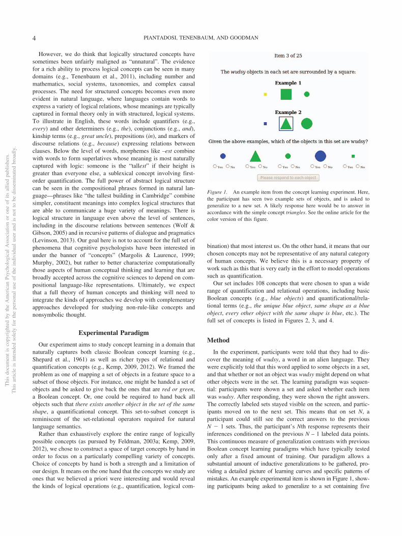
In the experiment, participants were told that they had to dis-cover the meaning of wudsy, a word in an alien language. Theywere explicitly told that this word applied to some objects in a set,and that whether or not an object was wudsy might depend on whatother objects were in the set. The learning paradigm was sequen-tial: participants were shown a set and asked whether each itemwas wudsy. After responding, they were shown the right answers.The correctly labeled sets stayed visible on the screen, and partic-ipants moved on to the next set. This means that on set N, aparticipant could still see the correct answers to the previousN � 1 sets. Thus, the participant’s Nth response represents theirinferences conditioned on the previous N – 1 labeled data points.This continuous measure of generalization contrasts with previousBoolean concept learning paradigms which have typically testedonly after a fixed amount of training. Our paradigm allows asubstantial amount of inductive generalizations to be gathered, pro-viding a detailed picture of learning curves and specific patterns ofmistakes. An example experimental item is shown in Figure 1, show-ing participants being asked to generalize to a set containing five

Figure 1. An example item from the concept learning experiment. Here,the participant has seen two example sets of objects, and is asked togeneralize to a new set. A likely response here would be to answer inaccordance with the simple concept triangles. See the online article for thecolor version of this figure.

Thi

sdo

cum

ent

isco

pyri

ghte

dby

the

Am

eric

anPs

ycho

logi

cal

Ass

ocia

tion

oron

eof

itsal

lied

publ

ishe

rs.

Thi

sar

ticle

isin

tend

edso

lely

for

the

pers

onal

use

ofth

ein

divi

dual

user

and

isno

tto

bedi

ssem

inat

edbr

oadl

y.


elements after seeing the two preceding sets, only one of whichcontained a positive instance of a wudsy object.

To aid in motivation, participants were required to wait 5 secondswhen they made a mistake in any element of a set. The space ofobjects included squares, circles, and triangles, that were green, blue,or yellow. Object sizes ranged through three logarithmically spacedsizes, denoted here Size 1 (smallest), 2, and 3 (largest). Sets weregenerated from this space of objects at random by first uniformlychoosing a set cardinality between 1 and 5, and then randomlysampling objects without replacement. Random generation was usedto ensure that participants do not assume sets were chosen to beinformative about target concepts (as in, e.g., Shafto & Goodman,2008). Subjects were shown 25 sets of objects in total, requiring onaverage a total of 75 responses to individual objects.

Subjects were randomly assigned to a concept and one of two listsin that concept, where each list was a different sequence labeledaccording to the target concept. Within the same list, the presentedsequence of data was identical. Subjects were allowed to do multipleconcepts, but could not repeat the same concept twice. The smallnumber of lists allowed us to run more participants within each list toget higher confidence in the exact learning curves for any particularsequence of labeled data. The specific shapes and colors in each targetconcept were randomized across participants. For example, red andcircle was randomized to blue and triangle, blue and square, greenand circle, and so forth across participants.

At sets 5, 10, and 25, participants were asked to describe what theythought wudsy meant. In general, verbal descriptions proved ex-tremely difficult to analyze because participants often wrote ambig-uous descriptions. For instance, we ran concepts such as the uniquetallest (cannot be tied for tallest shape in the set) and one of the tallest(can be tied for tallest shape in the set). Subjects with both of theseconcepts wrote “tallest,” which, in English, might mean either con-cept. While we do not analyze this linguistic data here, the ambiguityin participant descriptions provides some evidence that participantsdid not represent target concepts in natural language—doing so oftenleaves the target concept underspecified.

Subjects were run online using Amazon’s Mechanical Turk.Subjects who fell more than 2 standard deviations below the meanaccuracy in their concept were removed. This removed on averageonly 3.9% of data from each concept (standard deviation � 2.6%across concepts). Data from participants who completed fewerthan five sets of a given concept was also removed, but otherwisepartial data from participants was included in our analysis. A totalof 1,596 participants were run across the 108 concepts. While wedid not gather detailed demographics on subjects, a study of thepopulation of people who tend to complete Turk experiments canbe found in Berinsky, Huber, and Lenz (2012), who show that thestudy population is often more representative of the U.S. popula-tion than in-person convenience samples typically used in research(see also Paolacci, Chandler, & Ipeirotis, 2010; Behrend, Sharek,Meade, & Wiebe, 2011). In our experiment, individual participantscompleted an average of 4.24 concepts (median 2), with themaximum number of concepts run by a participant at 80. Overallaccuracy in the experiment was 78% with a chance rate of 56%,though the accuracies varied substantially by concept. Mean ac-curacies on concepts were highly consistent across the two lists,with a correlation of R2 � 0.81. Subjects were run until eachconcept and list was completed by approximately 20 participants.

Model-Free Results

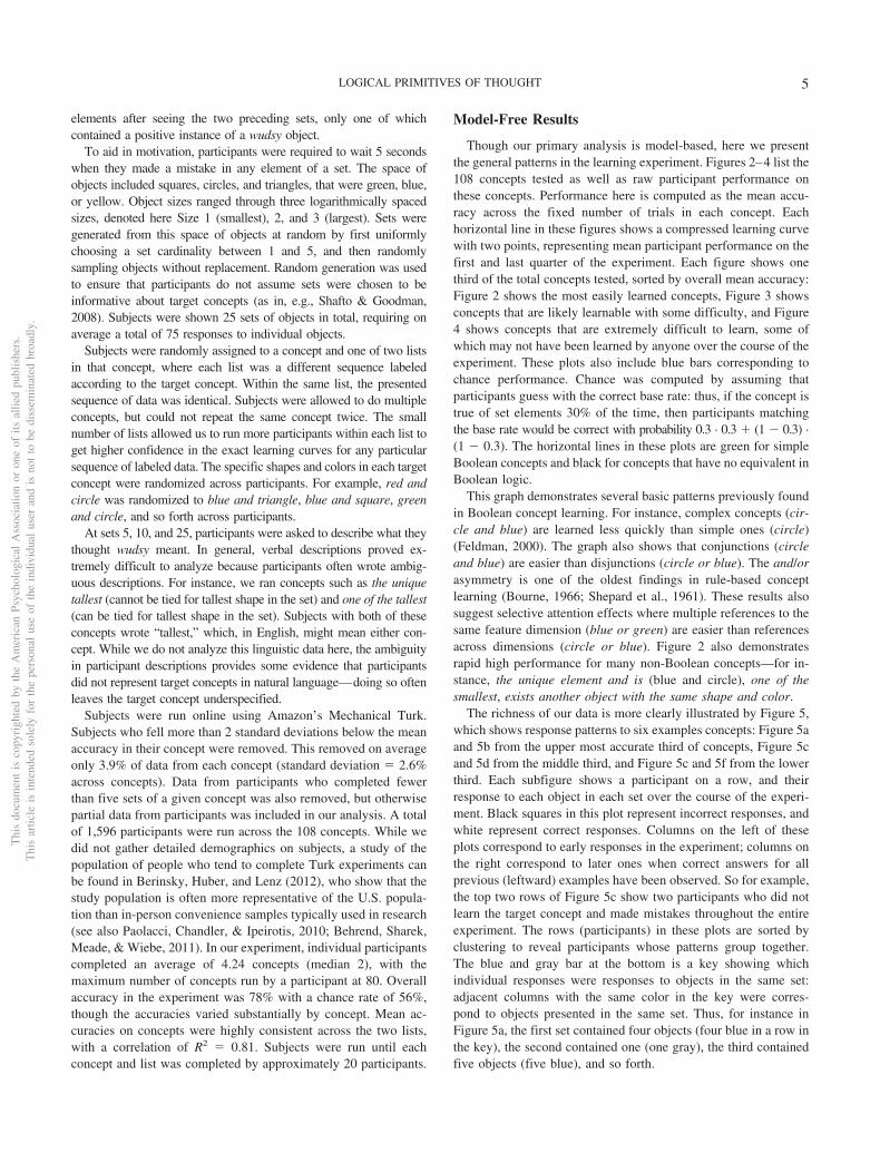
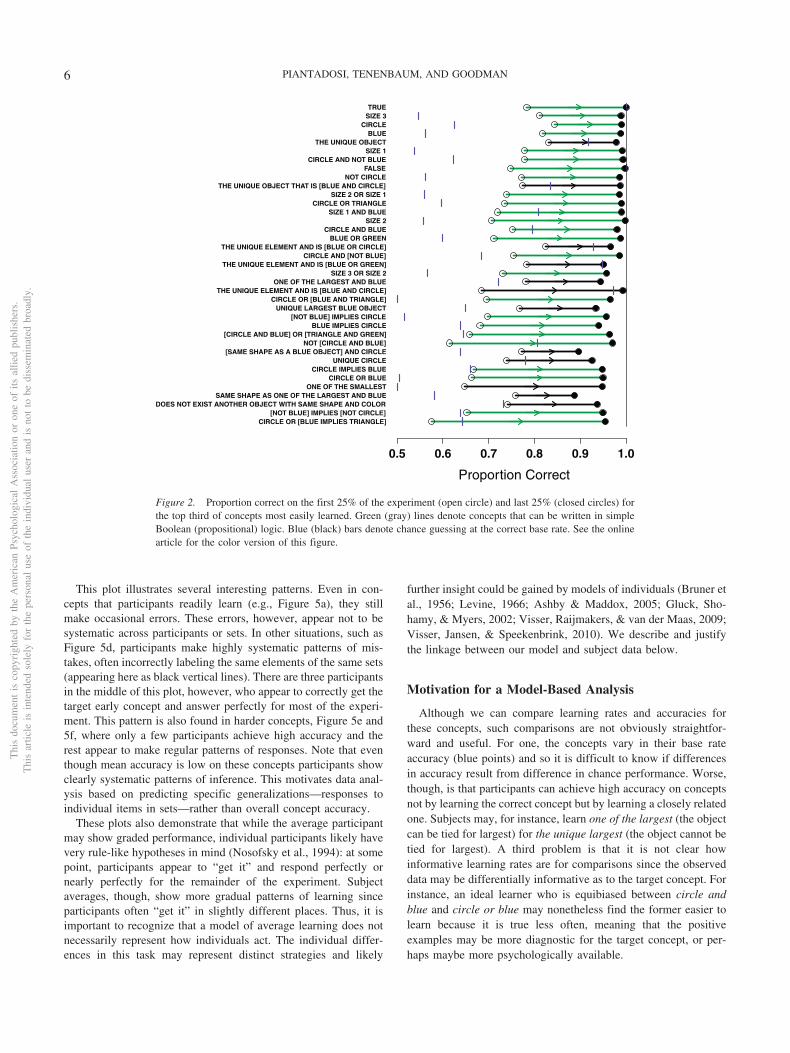
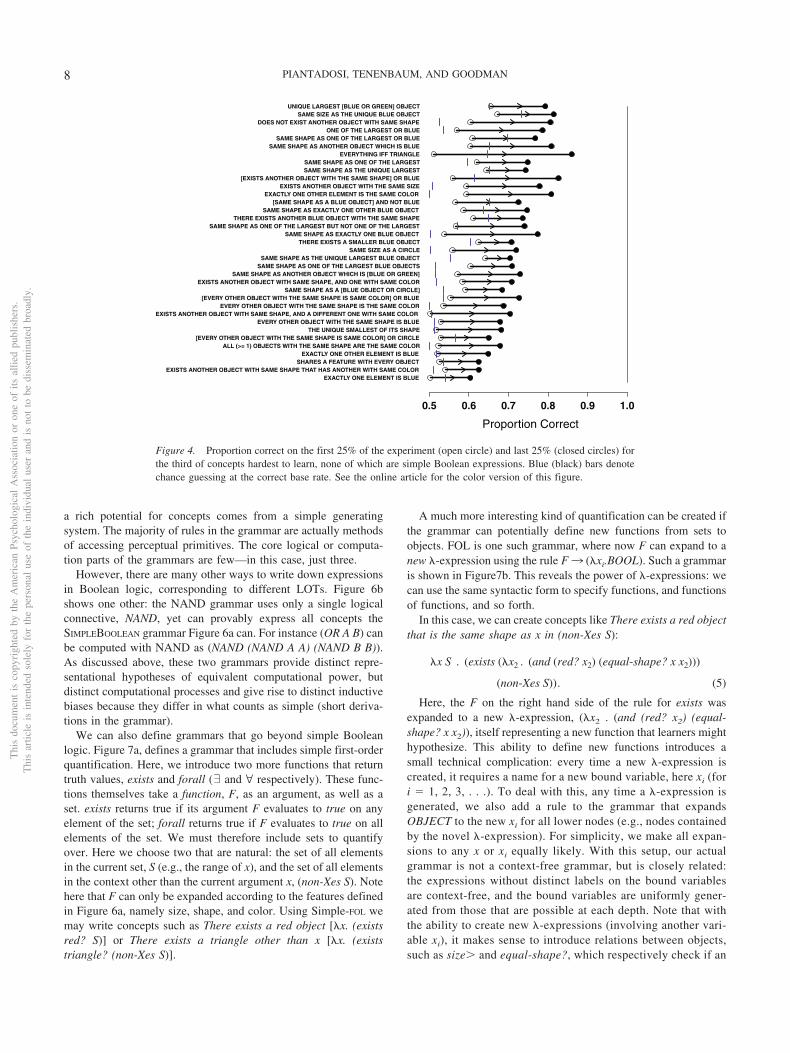
Though our primary analysis is model-based, here we presentthe general patterns in the learning experiment. Figures 2–4 list the108 concepts tested as well as raw participant performance onthese concepts. Performance here is computed as the mean accu-racy across the fixed number of trials in each concept. Eachhorizontal line in these figures shows a compressed learning curvewith two points, representing mean participant performance on thefirst and last quarter of the experiment. Each figure shows onethird of the total concepts tested, sorted by overall mean accuracy:Figure 2 shows the most easily learned concepts, Figure 3 showsconcepts that are likely learnable with some difficulty, and Figure4 shows concepts that are extremely difficult to learn, some ofwhich may not have been learned by anyone over the course of theexperiment. These plots also include blue bars corresponding tochance performance. Chance was computed by assuming thatparticipants guess with the correct base rate: thus, if the concept istrue of set elements 30% of the time, then participants matchingthe base rate would be correct with probability 0.3 · 0.3 � (1 � 0.3) ·(1 � 0.3). The horizontal lines in these plots are green for simpleBoolean concepts and black for concepts that have no equivalent inBoolean logic.

This graph demonstrates several basic patterns previously foundin Boolean concept learning. For instance, complex concepts (cir-cle and blue) are learned less quickly than simple ones (circle)(Feldman, 2000). The graph also shows that conjunctions (circleand blue) are easier than disjunctions (circle or blue). The and/orasymmetry is one of the oldest findings in rule-based conceptlearning (Bourne, 1966; Shepard et al., 1961). These results alsosuggest selective attention effects where multiple references to thesame feature dimension (blue or green) are easier than referencesacross dimensions (circle or blue). Figure 2 also demonstratesrapid high performance for many non-Boolean concepts—for in-stance, the unique element and is (blue and circle), one of thesmallest, exists another object with the same shape and color.

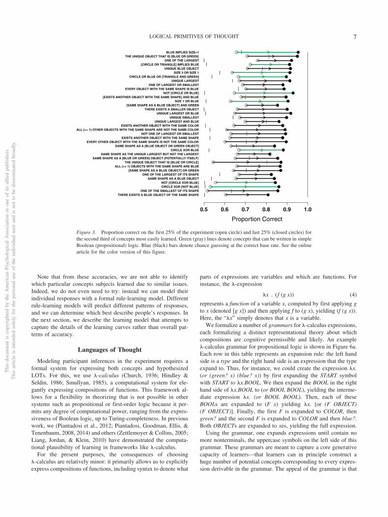
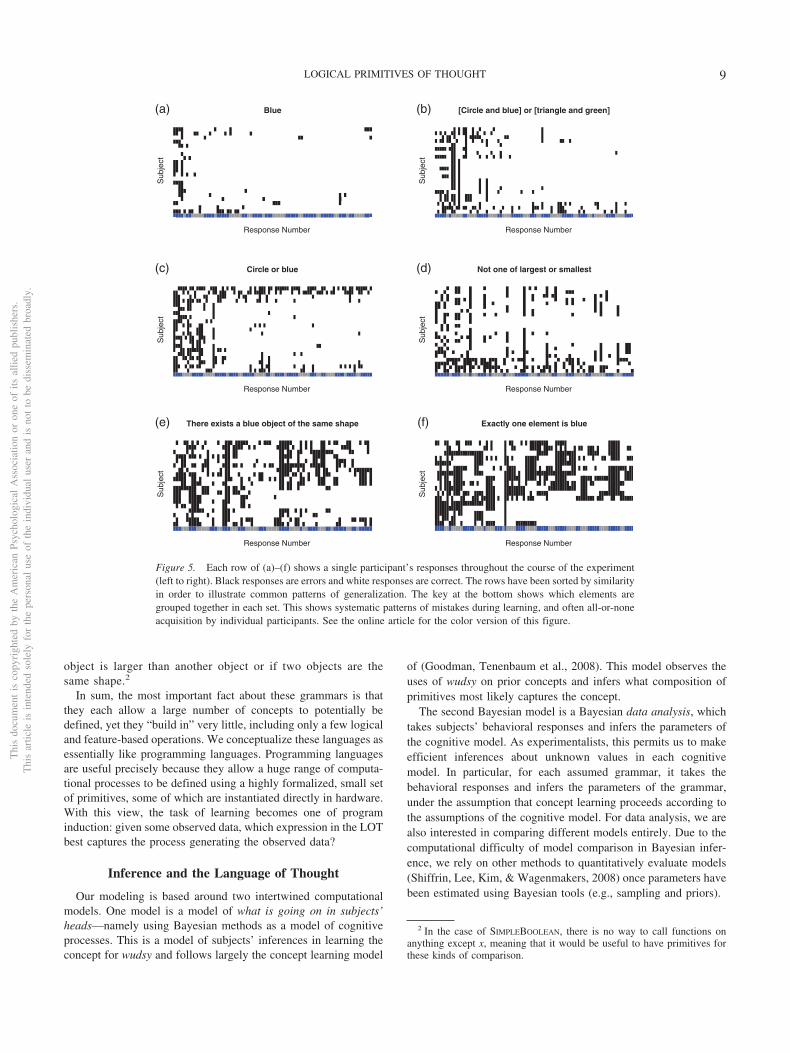
The richness of our data is more clearly illustrated by Figure 5,which shows response patterns to six examples concepts: Figure 5aand 5b from the upper most accurate third of concepts, Figure 5cand 5d from the middle third, and Figure 5c and 5f from the lowerthird. Each subfigure shows a participant on a row, and theirresponse to each object in each set over the course of the experi-ment. Black squares in this plot represent incorrect responses, andwhite represent correct responses. Columns on the left of theseplots correspond to early responses in the experiment; columns onthe right correspond to later ones when correct answers for allprevious (leftward) examples have been observed. So for example,the top two rows of Figure 5c show two participants who did notlearn the target concept and made mistakes throughout the entireexperiment. The rows (participants) in these plots are sorted byclustering to reveal participants whose patterns group together.The blue and gray bar at the bottom is a key showing whichindividual responses were responses to objects in the same set:adjacent columns with the same color in the key were corres-pond to objects presented in the same set. Thus, for instance inFigure 5a, the first set contained four objects (four blue in a row inthe key), the second contained one (one gray), the third containedfive objects (five blue), and so forth.

Thi

sdo

cum

ent

isco

pyri

ghte

dby

the

Am

eric

anPs

ycho

logi

cal

Ass

ocia

tion

oron

eof

itsal

lied

publ

ishe

rs.

Thi

sar

ticle

isin

tend

edso

lely

for

the

pers

onal

use

ofth

ein

divi

dual

user

and

isno

tto

bedi

ssem

inat

edbr

oadl

y.


This plot illustrates several interesting patterns. Even in con-cepts that participants readily learn (e.g., Figure 5a), they stillmake occasional errors. These errors, however, appear not to besystematic across participants or sets. In other situations, such asFigure 5d, participants make highly systematic patterns of mis-takes, often incorrectly labeling the same elements of the same sets(appearing here as black vertical lines). There are three participantsin the middle of this plot, however, who appear to correctly get thetarget early concept and answer perfectly for most of the experi-ment. This pattern is also found in harder concepts, Figure 5e and5f, where only a few participants achieve high accuracy and therest appear to make regular patterns of responses. Note that eventhough mean accuracy is low on these concepts participants showclearly systematic patterns of inference. This motivates data anal-ysis based on predicting specific generalizations—responses toindividual items in sets—rather than overall concept accuracy.

These plots also demonstrate that while the average participantmay show graded performance, individual participants likely havevery rule-like hypotheses in mind (Nosofsky et al., 1994): at somepoint, participants appear to “get it” and respond perfectly ornearly perfectly for the remainder of the experiment. Subjectaverages, though, show more gradual patterns of learning sinceparticipants often “get it” in slightly different places. Thus, it isimportant to recognize that a model of average learning does notnecessarily represent how individuals act. The individual differ-ences in this task may represent distinct strategies and likely

further insight could be gained by models of individuals (Bruner etal., 1956; Levine, 1966; Ashby & Maddox, 2005; Gluck, Sho-hamy, & Myers, 2002; Visser, Raijmakers, & van der Maas, 2009;Visser, Jansen, & Speekenbrink, 2010). We describe and justifythe linkage between our model and subject data below.

Motivation for a Model-Based Analysis

Although we can compare learning rates and accuracies forthese concepts, such comparisons are not obviously straightfor-ward and useful. For one, the concepts vary in their base rateaccuracy (blue points) and so it is difficult to know if differencesin accuracy result from difference in chance performance. Worse,though, is that participants can achieve high accuracy on conceptsnot by learning the correct concept but by learning a closely relatedone. Subjects may, for instance, learn one of the largest (the objectcan be tied for largest) for the unique largest (the object cannot betied for largest). A third problem is that it is not clear howinformative learning rates are for comparisons since the observeddata may be differentially informative as to the target concept. Forinstance, an ideal learner who is equibiased between circle andblue and circle or blue may nonetheless find the former easier tolearn because it is true less often, meaning that the positiveexamples may be more diagnostic for the target concept, or per-haps maybe more psychologically available.

CIRCLE OR [BLUE IMPLIES TRIANGLE][NOT BLUE] IMPLIES [NOT CIRCLE]

DOES NOT EXIST ANOTHER OBJECT WITH SAME SHAPE AND COLORSAME SHAPE AS ONE OF THE LARGEST AND BLUE

ONE OF THE SMALLESTCIRCLE OR BLUE

CIRCLE IMPLIES BLUEUNIQUE CIRCLE

[SAME SHAPE AS A BLUE OBJECT] AND CIRCLENOT [CIRCLE AND BLUE]

[CIRCLE AND BLUE] OR [TRIANGLE AND GREEN]BLUE IMPLIES CIRCLE

[NOT BLUE] IMPLIES CIRCLEUNIQUE LARGEST BLUE OBJECT

CIRCLE OR [BLUE AND TRIANGLE]THE UNIQUE ELEMENT AND IS [BLUE AND CIRCLE]

ONE OF THE LARGEST AND BLUESIZE 3 OR SIZE 2

THE UNIQUE ELEMENT AND IS [BLUE OR GREEN]CIRCLE AND [NOT BLUE]

THE UNIQUE ELEMENT AND IS [BLUE OR CIRCLE]BLUE OR GREEN

CIRCLE AND BLUESIZE 2

SIZE 1 AND BLUECIRCLE OR TRIANGLE

SIZE 2 OR SIZE 1THE UNIQUE OBJECT THAT IS [BLUE AND CIRCLE]

NOT CIRCLEFALSE

CIRCLE AND NOT BLUESIZE 1

THE UNIQUE OBJECTBLUE

CIRCLESIZE 3TRUE

Proportion Correct

0.5 0.6 0.7 0.8 0.9 1.0

Figure 2. Proportion correct on the first 25% of the experiment (open circle) and last 25% (closed circles) forthe top third of concepts most easily learned. Green (gray) lines denote concepts that can be written in simpleBoolean (propositional) logic. Blue (black) bars denote chance guessing at the correct base rate. See the onlinearticle for the color version of this figure.

Thi

sdo

cum

ent

isco

pyri

ghte

dby

the

Am

eric

anPs

ycho

logi

cal

Ass

ocia

tion

oron

eof

itsal

lied

publ

ishe

rs.

Thi

sar

ticle

isin

tend

edso

lely

for

the

pers

onal

use

ofth

ein

divi

dual

user

and

isno

tto

bedi

ssem

inat

edbr

oadl

y.


Note that from these accuracies, we are not able to identifywhich particular concepts subjects learned due to similar issues.Indeed, we do not even need to try: instead we can model theirindividual responses with a formal rule-learning model. Differentrule-learning models will predict different patterns of responses,and we can determine which best describe people’s responses. Inthe next section, we describe the learning model that attempts tocapture the details of the learning curves rather than overall pat-terns of accuracy.

Languages of Thought

Modeling participant inferences in the experiment requires aformal system for expressing both concepts and hypothesizedLOTs. For this, we use �-calculus (Church, 1936; Hindley &Seldin, 1986; Smullyan, 1985), a computational system for ele-gantly expressing compositions of functions. This framework al-lows for a flexibility in theorizing that is not possible in othersystems such as propositional or first-order logic because it per-mits any degree of computational power, ranging from the expres-siveness of Boolean logic, up to Turing-completeness. In previouswork, we (Piantadosi et al., 2012; Piantadosi, Goodman, Ellis, &Tenenbaum, 2008, 2014) and others (Zettlemoyer & Collins, 2005;Liang, Jordan, & Klein, 2010) have demonstrated the computa-tional plausibility of learning in frameworks like �-calculus.

For the present purposes, the consequences of choosing�-calculus are relatively minor: it primarily allows us to explicitlyexpress compositions of functions, including syntax to denote what

parts of expressions are variables and which are functions. Forinstance, the �-expression

�x . (f (g x)) (4)

represents a function of a variable x, computed by first applying gto x (denoted [g x]) and then applying f to (g x), yielding (f (g x)).Here, the “�x” simply denotes that x is a variable.

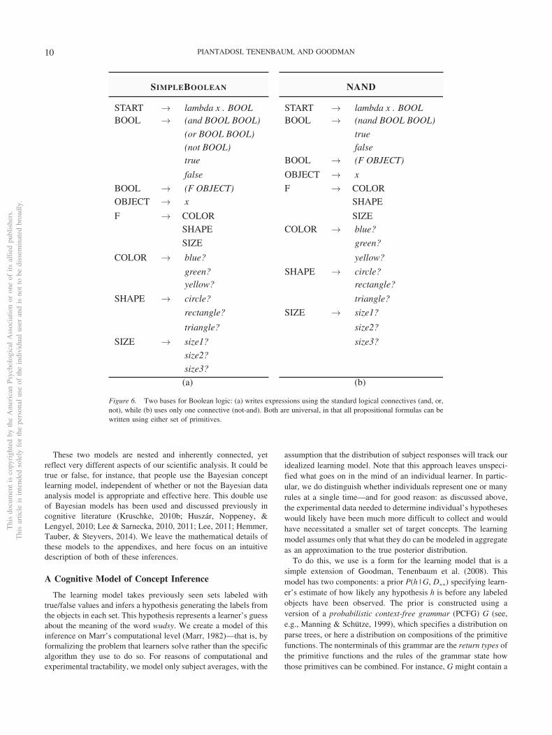
We formalize a number of grammars for �-calculus expressions,each formalizing a distinct representational theory about whichcompositions are cognitive permissible and likely. An example�-calculus grammar for propositional logic is shown in Figure 6a.Each row in this table represents an expansion rule: the left handside is a type and the right hand side is an expression that the typeexpand to. Thus, for instance, we could create the expression �x.(or (green? x) (blue? x)) by first expanding the START symbolwith START to �x.BOOL. We then expand the BOOL in the righthand side of �x.BOOL to (or BOOL BOOL), yielding the interme-diate expression �x. (or BOOL BOOL). Then, each of theseBOOLs are expanded to (F x) yielding �x. [or (F OBJECT)(F OBJECT)]. Finally, the first F is expanded to COLOR, thengreen? and the second F is expanded to COLOR and then blue?.Both OBJECTs are expanded to xes, yielding the full expression.

Using the grammar, one expands expressions until contain nomore nonterminals, the uppercase symbols on the left side of thisgrammar. These grammars are meant to capture a core generativecapacity of learners—that learners can in principle construct ahuge number of potential concepts corresponding to every expres-sion derivable in the grammar. The appeal of the grammar is that

THERE EXISTS A BLUE OBJECT OF THE SAME SHAPEONE OF THE SMALLEST OF ITS SHAPE

CIRCLE XOR [NOT BLUE]NOT [CIRCLE XOR BLUE]

SAME SHAPE AS A BLUE OBJECTONE OF THE LARGEST OF ITS SHAPE

[SAME SHAPE AS A BLUE OBJECT] OR GREENALL (>= 1) OBJECTS WITH THE SAME SHAPE ARE BLUE

THE UNIQUE OBJECT THAT IS [BLUE OR CIRCLE]SAME SHAPE AS A [BLUE OR GREEN] OBJECT (POTENTIALLY ITSELF)

SAME SHAPE AS THE UNIQUE LARGEST BUT NOT THE LARGESTCIRCLE XOR BLUE

SAME SHAPE AS A [BLUE OBJECT OR GREEN OBJECT]EVERY OTHER OBJECT WITH THE SAME SHAPE IS NOT THE SAME COLOR

EXISTS ANOTHER OBJECT WITH THE SAME SHAPENOT ONE OF LARGEST OR SMALLEST

ALL (>= 1) OTHER OBJECTS WITH THE SAME SHAPE ARE NOT THE SAME COLOREXISTS ANOTHER OBJECT WITH THE SAME COLOR

UNIQUE LARGEST AND BLUEUNIQUE SMALLEST

UNIQUE LARGEST OR BLUETHERE EXISTS A SMALLER OBJECT

[SAME SHAPE AS A BLUE OBJECT] AND GREENSIZE 1 OR BLUE

[EXISTS ANOTHER OBJECT WITH THE SAME SHAPE] AND BLUENOT [CIRCLE OR BLUE]

EVERY OBJECT WITH THE SAME SHAPE IS BLUEONE OF LARGEST OR SMALLEST

UNIQUE LARGESTCIRCLE OR BLUE OR [TRIANGLE AND GREEN]

SIZE 3 OR SIZE 1UNIQUE BLUE OBJECT

[CIRCLE OR TRIANGLE] IMPLIES BLUEONE OF THE LARGEST

THE UNIQUE OBJECT THAT IS [BLUE OR GREEN]BLUE IMPLIES SIZE=1

Proportion Correct

0.5 0.6 0.7 0.8 0.9 1.0

Figure 3. Proportion correct on the first 25% of the experiment (open circle) and last 25% (closed circles) forthe second third of concepts most easily learned. Green (gray) lines denote concepts that can be written in simpleBoolean (propositional) logic. Blue (black) bars denote chance guessing at the correct base rate. See the onlinearticle for the color version of this figure.

Thi

sdo

cum

ent

isco

pyri

ghte

dby

the

Am

eric

anPs

ycho

logi

cal

Ass

ocia

tion

oron

eof

itsal

lied

publ

ishe

rs.

Thi

sar

ticle

isin

tend

edso

lely

for

the

pers

onal

use

ofth

ein

divi

dual

user

and

isno

tto

bedi

ssem

inat

edbr

oadl

y.


a rich potential for concepts comes from a simple generatingsystem. The majority of rules in the grammar are actually methodsof accessing perceptual primitives. The core logical or computa-tion parts of the grammars are few—in this case, just three.

However, there are many other ways to write down expressionsin Boolean logic, corresponding to different LOTs. Figure 6bshows one other: the NAND grammar uses only a single logicalconnective, NAND, yet can provably express all concepts theSIMPLEBOOLEAN grammar Figure 6a can. For instance (OR A B) canbe computed with NAND as (NAND (NAND A A) (NAND B B)).As discussed above, these two grammars provide distinct repre-sentational hypotheses of equivalent computational power, butdistinct computational processes and give rise to distinct inductivebiases because they differ in what counts as simple (short deriva-tions in the grammar).

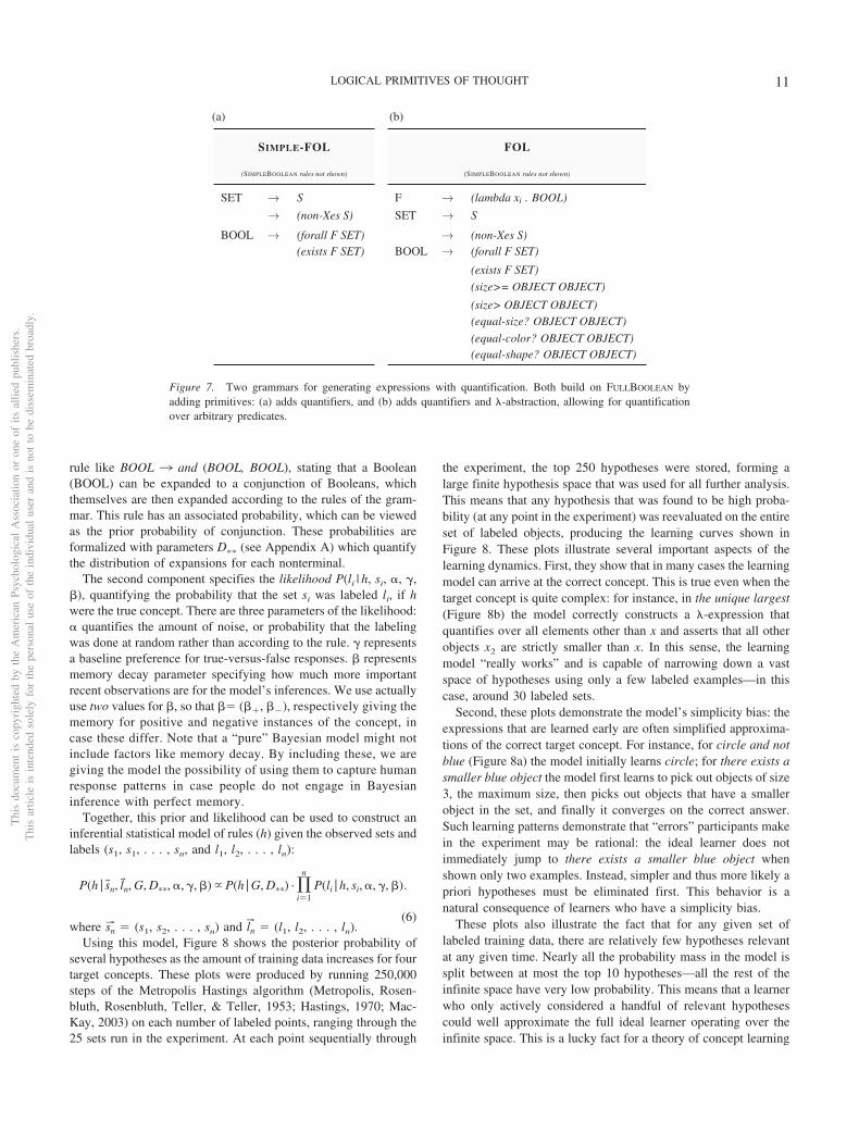
We can also define grammars that go beyond simple Booleanlogic. Figure 7a, defines a grammar that includes simple first-orderquantification. Here, we introduce two more functions that returntruth values, exists and forall (? and @ respectively). These func-tions themselves take a function, F, as an argument, as well as aset. exists returns true if its argument F evaluates to true on anyelement of the set; forall returns true if F evaluates to true on allelements of the set. We must therefore include sets to quantifyover. Here we choose two that are natural: the set of all elementsin the current set, S (e.g., the range of x), and the set of all elementsin the context other than the current argument x, (non-Xes S). Notehere that F can only be expanded according to the features definedin Figure 6a, namely size, shape, and color. Using Simple-FOL wemay write concepts such as There exists a red object [�x. (existsred? S)] or There exists a triangle other than x [�x. (existstriangle? (non-Xes S)].

A much more interesting kind of quantification can be created ifthe grammar can potentially define new functions from sets toobjects. FOL is one such grammar, where now F can expand to anew �-expression using the rule F ¡ (�xi.BOOL). Such a grammaris shown in Figure7b. This reveals the power of �-expressions: wecan use the same syntactic form to specify functions, and functionsof functions, and so forth.

In this case, we can create concepts like There exists a red objectthat is the same shape as x in (non-Xes S):

�x S . (exists (�x2 . (and (red? x2) (equal-shape? x x2)))

(non-Xes S)). (5)

Here, the F on the right hand side of the rule for exists wasexpanded to a new �-expression, (�x2 . (and (red? x2) (equal-shape? x x2)), itself representing a new function that learners mighthypothesize. This ability to define new functions introduces asmall technical complication: every time a new �-expression iscreated, it requires a name for a new bound variable, here xi (fori � 1, 2, 3, . . .). To deal with this, any time a �-expression isgenerated, we also add a rule to the grammar that expandsOBJECT to the new xi for all lower nodes (e.g., nodes containedby the novel �-expression). For simplicity, we make all expan-sions to any x or xi equally likely. With this setup, our actualgrammar is not a context-free grammar, but is closely related:the expressions without distinct labels on the bound variablesare context-free, and the bound variables are uniformly gener-ated from those that are possible at each depth. Note that withthe ability to create new �-expressions (involving another vari-able xi), it makes sense to introduce relations between objects,such as size� and equal-shape?, which respectively check if an

EXACTLY ONE ELEMENT IS BLUEEXISTS ANOTHER OBJECT WITH SAME SHAPE THAT HAS ANOTHER WITH SAME COLOR

SHARES A FEATURE WITH EVERY OBJECTEXACTLY ONE OTHER ELEMENT IS BLUE

ALL (>= 1) OBJECTS WITH THE SAME SHAPE ARE THE SAME COLOR[EVERY OTHER OBJECT WITH THE SAME SHAPE IS SAME COLOR] OR CIRCLE

THE UNIQUE SMALLEST OF ITS SHAPEEVERY OTHER OBJECT WITH THE SAME SHAPE IS BLUE

EXISTS ANOTHER OBJECT WITH SAME SHAPE, AND A DIFFERENT ONE WITH SAME COLOR EVERY OTHER OBJECT WITH THE SAME SHAPE IS THE SAME COLOR

[EVERY OTHER OBJECT WITH THE SAME SHAPE IS SAME COLOR] OR BLUESAME SHAPE AS A [BLUE OBJECT OR CIRCLE]

EXISTS ANOTHER OBJECT WITH SAME SHAPE, AND ONE WITH SAME COLORSAME SHAPE AS ANOTHER OBJECT WHICH IS [BLUE OR GREEN]

SAME SHAPE AS ONE OF THE LARGEST BLUE OBJECTSSAME SHAPE AS THE UNIQUE LARGEST BLUE OBJECT

SAME SIZE AS A CIRCLETHERE EXISTS A SMALLER BLUE OBJECT

SAME SHAPE AS EXACTLY ONE BLUE OBJECTSAME SHAPE AS ONE OF THE LARGEST BUT NOT ONE OF THE LARGEST

THERE EXISTS ANOTHER BLUE OBJECT WITH THE SAME SHAPESAME SHAPE AS EXACTLY ONE OTHER BLUE OBJECT

[SAME SHAPE AS A BLUE OBJECT] AND NOT BLUEEXACTLY ONE OTHER ELEMENT IS THE SAME COLOR

EXISTS ANOTHER OBJECT WITH THE SAME SIZE[EXISTS ANOTHER OBJECT WITH THE SAME SHAPE] OR BLUE

SAME SHAPE AS THE UNIQUE LARGESTSAME SHAPE AS ONE OF THE LARGEST

EVERYTHING IFF TRIANGLESAME SHAPE AS ANOTHER OBJECT WHICH IS BLUE

SAME SHAPE AS ONE OF THE LARGEST OR BLUEONE OF THE LARGEST OR BLUE

DOES NOT EXIST ANOTHER OBJECT WITH SAME SHAPESAME SIZE AS THE UNIQUE BLUE OBJECT

UNIQUE LARGEST [BLUE OR GREEN] OBJECT

Proportion Correct

0.5 0.6 0.7 0.8 0.9 1.0

Figure 4. Proportion correct on the first 25% of the experiment (open circle) and last 25% (closed circles) forthe third of concepts hardest to learn, none of which are simple Boolean expressions. Blue (black) bars denotechance guessing at the correct base rate. See the online article for the color version of this figure.

Thi

sdo

cum

ent

isco

pyri

ghte

dby

the

Am

eric

anPs

ycho

logi

cal

Ass

ocia

tion

oron

eof

itsal

lied

publ

ishe

rs.

Thi

sar

ticle

isin

tend

edso

lely

for

the

pers

onal

use

ofth

ein

divi

dual

user

and

isno

tto

bedi

ssem

inat

edbr

oadl

y.


object is larger than another object or if two objects are thesame shape.2

In sum, the most important fact about these grammars is thatthey each allow a large number of concepts to potentially bedefined, yet they “build in” very little, including only a few logicaland feature-based operations. We conceptualize these languages asessentially like programming languages. Programming languagesare useful precisely because they allow a huge range of computa-tional processes to be defined using a highly formalized, small setof primitives, some of which are instantiated directly in hardware.With this view, the task of learning becomes one of programinduction: given some observed data, which expression in the LOTbest captures the process generating the observed data?

Inference and the Language of Thought

Our modeling is based around two intertwined computationalmodels. One model is a model of what is going on in subjects’heads—namely using Bayesian methods as a model of cognitiveprocesses. This is a model of subjects’ inferences in learning theconcept for wudsy and follows largely the concept learning model

of (Goodman, Tenenbaum et al., 2008). This model observes theuses of wudsy on prior concepts and infers what composition ofprimitives most likely captures the concept.

The second Bayesian model is a Bayesian data analysis, whichtakes subjects’ behavioral responses and infers the parameters ofthe cognitive model. As experimentalists, this permits us to makeefficient inferences about unknown values in each cognitivemodel. In particular, for each assumed grammar, it takes thebehavioral responses and infers the parameters of the grammar,under the assumption that concept learning proceeds according tothe assumptions of the cognitive model. For data analysis, we arealso interested in comparing different models entirely. Due to thecomputational difficulty of model comparison in Bayesian infer-ence, we rely on other methods to quantitatively evaluate models(Shiffrin, Lee, Kim, & Wagenmakers, 2008) once parameters havebeen estimated using Bayesian tools (e.g., sampling and priors).

2 In the case of SIMPLEBOOLEAN, there is no way to call functions onanything except x, meaning that it would be useful to have primitives forthese kinds of comparison.

Blue

Response Number

Sub

ject

(a) [Circle and blue] or [triangle and green]

Response Number

Sub

ject

(b)

Circle or blue

Response Number

Sub

ject

(c) Not one of largest or smallest

Response Number

Sub

ject

(d)

There exists a blue object of the same shape

Response Number

Sub

ject

(e) Exactly one element is blue

Response Number

Sub

ject

(f)

Figure 5. Each row of (a)–(f) shows a single participant’s responses throughout the course of the experiment(left to right). Black responses are errors and white responses are correct. The rows have been sorted by similarityin order to illustrate common patterns of generalization. The key at the bottom shows which elements aregrouped together in each set. This shows systematic patterns of mistakes during learning, and often all-or-noneacquisition by individual participants. See the online article for the color version of this figure.

Thi

sdo

cum

ent

isco

pyri

ghte

dby

the

Am

eric

anPs

ycho

logi

cal

Ass

ocia

tion

oron

eof

itsal

lied

publ

ishe

rs.

Thi

sar

ticle

isin

tend

edso

lely

for

the

pers

onal

use

ofth

ein

divi

dual

user

and

isno

tto

bedi

ssem

inat

edbr

oadl

y.


These two models are nested and inherently connected, yetreflect very different aspects of our scientific analysis. It could betrue or false, for instance, that people use the Bayesian conceptlearning model, independent of whether or not the Bayesian dataanalysis model is appropriate and effective here. This double useof Bayesian models has been used and discussed previously incognitive literature (Kruschke, 2010b; Huszár, Noppeney, &Lengyel, 2010; Lee & Sarnecka, 2010, 2011; Lee, 2011; Hemmer,Tauber, & Steyvers, 2014). We leave the mathematical details ofthese models to the appendixes, and here focus on an intuitivedescription of both of these inferences.

A Cognitive Model of Concept Inference

The learning model takes previously seen sets labeled withtrue/false values and infers a hypothesis generating the labels fromthe objects in each set. This hypothesis represents a learner’s guessabout the meaning of the word wudsy. We create a model of thisinference on Marr’s computational level (Marr, 1982)—that is, byformalizing the problem that learners solve rather than the specificalgorithm they use to do so. For reasons of computational andexperimental tractability, we model only subject averages, with the

assumption that the distribution of subject responses will track ouridealized learning model. Note that this approach leaves unspeci-fied what goes on in the mind of an individual learner. In partic-ular, we do distinguish whether individuals represent one or manyrules at a single time—and for good reason: as discussed above,the experimental data needed to determine individual’s hypotheseswould likely have been much more difficult to collect and wouldhave necessitated a smaller set of target concepts. The learningmodel assumes only that what they do can be modeled in aggregateas an approximation to the true posterior distribution.

To do this, we use is a form for the learning model that is asimple extension of Goodman, Tenenbaum et al. (2008). Thismodel has two components: a prior P(h | G, D��) specifying learn-er’s estimate of how likely any hypothesis h is before any labeledobjects have been observed. The prior is constructed using aversion of a probabilistic context-free grammar (PCFG) G (see,e.g., Manning & Schütze, 1999), which specifies a distribution onparse trees, or here a distribution on compositions of the primitivefunctions. The nonterminals of this grammar are the return types ofthe primitive functions and the rules of the grammar state howthose primitives can be combined. For instance, G might contain a

Figure 6. Two bases for Boolean logic: (a) writes expressions using the standard logical connectives (and, or,not), while (b) uses only one connective (not-and). Both are universal, in that all propositional formulas can bewritten using either set of primitives.

Thi

sdo

cum

ent

isco

pyri

ghte

dby

the

Am

eric

anPs

ycho

logi

cal

Ass

ocia

tion

oron

eof

itsal

lied

publ

ishe

rs.

Thi

sar

ticle

isin

tend

edso

lely

for

the

pers

onal

use

ofth

ein

divi

dual

user

and

isno

tto

bedi

ssem

inat

edbr

oadl

y.


rule like BOOL ¡ and (BOOL, BOOL), stating that a Boolean(BOOL) can be expanded to a conjunction of Booleans, whichthemselves are then expanded according to the rules of the gram-mar. This rule has an associated probability, which can be viewedas the prior probability of conjunction. These probabilities areformalized with parameters D�� (see Appendix A) which quantifythe distribution of expansions for each nonterminal.

The second component specifies the likelihood P(li | h, si, �, �,), quantifying the probability that the set si was labeled li, if hwere the true concept. There are three parameters of the likelihood:� quantifies the amount of noise, or probability that the labelingwas done at random rather than according to the rule. � representsa baseline preference for true-versus-false responses. representsmemory decay parameter specifying how much more importantrecent observations are for the model’s inferences. We use actuallyuse two values for , so that � (�, �), respectively giving thememory for positive and negative instances of the concept, incase these differ. Note that a “pure” Bayesian model might notinclude factors like memory decay. By including these, we aregiving the model the possibility of using them to capture humanresponse patterns in case people do not engage in Bayesianinference with perfect memory.

Together, this prior and likelihood can be used to construct aninferential statistical model of rules (h) given the observed sets andlabels (s1, s1, . . . , sn, and l1, l2, . . . , ln):

P(h | s�n, �ln, G, D��, �, �, �) � P(h | G, D��) · �i�1

n

P(li | h, si, �, �, �).

(6)where sn� � (s1, s2, . . . , sn) and ln� � (l1, l2, . . . , ln).

Using this model, Figure 8 shows the posterior probability ofseveral hypotheses as the amount of training data increases for fourtarget concepts. These plots were produced by running 250,000steps of the Metropolis Hastings algorithm (Metropolis, Rosen-bluth, Rosenbluth, Teller, & Teller, 1953; Hastings, 1970; Mac-Kay, 2003) on each number of labeled points, ranging through the25 sets run in the experiment. At each point sequentially through

the experiment, the top 250 hypotheses were stored, forming alarge finite hypothesis space that was used for all further analysis.This means that any hypothesis that was found to be high proba-bility (at any point in the experiment) was reevaluated on the entireset of labeled objects, producing the learning curves shown inFigure 8. These plots illustrate several important aspects of thelearning dynamics. First, they show that in many cases the learningmodel can arrive at the correct concept. This is true even when thetarget concept is quite complex: for instance, in the unique largest(Figure 8b) the model correctly constructs a �-expression thatquantifies over all elements other than x and asserts that all otherobjects x2 are strictly smaller than x. In this sense, the learningmodel “really works” and is capable of narrowing down a vastspace of hypotheses using only a few labeled examples—in thiscase, around 30 labeled sets.

Second, these plots demonstrate the model’s simplicity bias: theexpressions that are learned early are often simplified approxima-tions of the correct target concept. For instance, for circle and notblue (Figure 8a) the model initially learns circle; for there exists asmaller blue object the model first learns to pick out objects of size3, the maximum size, then picks out objects that have a smallerobject in the set, and finally it converges on the correct answer.Such learning patterns demonstrate that “errors” participants makein the experiment may be rational: the ideal learner does notimmediately jump to there exists a smaller blue object whenshown only two examples. Instead, simpler and thus more likely apriori hypotheses must be eliminated first. This behavior is anatural consequence of learners who have a simplicity bias.

These plots also illustrate the fact that for any given set oflabeled training data, there are relatively few hypotheses relevantat any given time. Nearly all the probability mass in the model issplit between at most the top 10 hypotheses—all the rest of theinfinite space have very low probability. This means that a learnerwho only actively considered a handful of relevant hypothesescould well approximate the full ideal learner operating over theinfinite space. This is a lucky fact for a theory of concept learning

Figure 7. Two grammars for generating expressions with quantification. Both build on FULLBOOLEAN byadding primitives: (a) adds quantifiers, and (b) adds quantifiers and �-abstraction, allowing for quantificationover arbitrary predicates.

Thi

sdo

cum

ent

isco

pyri

ghte

dby

the

Am

eric

anPs

ycho

logi

cal

Ass

ocia

tion

oron

eof

itsal

lied

publ

ishe

rs.

Thi

sar

ticle

isin

tend

edso

lely

for

the

pers

onal

use

ofth

ein

divi

dual

user

and

isno

tto

bedi

ssem

inat

edbr

oadl

y.


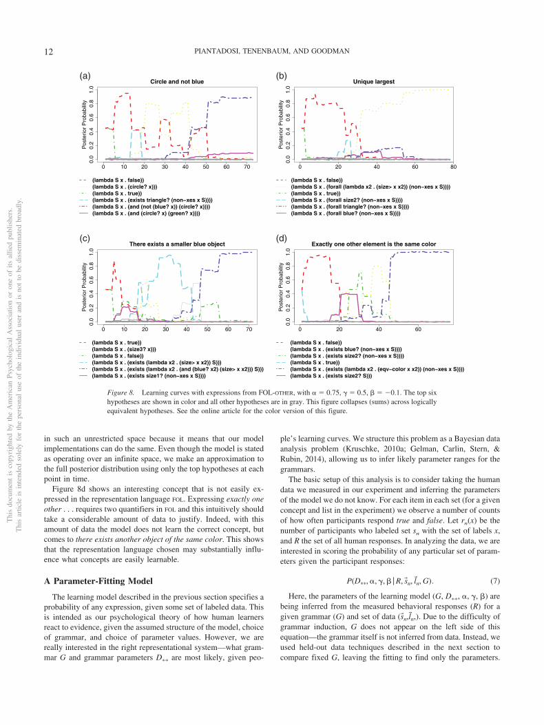
in such an unrestricted space because it means that our modelimplementations can do the same. Even though the model is statedas operating over an infinite space, we make an approximation tothe full posterior distribution using only the top hypotheses at eachpoint in time.

Figure 8d shows an interesting concept that is not easily ex-pressed in the representation language FOL. Expressing exactly oneother . . . requires two quantifiers in FOL and this intuitively shouldtake a considerable amount of data to justify. Indeed, with thisamount of data the model does not learn the correct concept, butcomes to there exists another object of the same color. This showsthat the representation language chosen may substantially influ-ence what concepts are easily learnable.

A Parameter-Fitting Model

The learning model described in the previous section specifies aprobability of any expression, given some set of labeled data. Thisis intended as our psychological theory of how human learnersreact to evidence, given the assumed structure of the model, choiceof grammar, and choice of parameter values. However, we arereally interested in the right representational system—what gram-mar G and grammar parameters D�� are most likely, given peo-

ple’s learning curves. We structure this problem as a Bayesian dataanalysis problem (Kruschke, 2010a; Gelman, Carlin, Stern, &Rubin, 2014), allowing us to infer likely parameter ranges for thegrammars.

The basic setup of this analysis is to consider taking the humandata we measured in our experiment and inferring the parametersof the model we do not know. For each item in each set (for a givenconcept and list in the experiment) we observe a number of countsof how often participants respond true and false. Let rn(x) be thenumber of participants who labeled set sn with the set of labels x,and R the set of all human responses. In analyzing the data, we areinterested in scoring the probability of any particular set of param-eters given the participant responses:

P(D��, �, �, � | R, s�n, �ln, G). (7)

Here, the parameters of the learning model (G, D��, �, �, ) arebeing inferred from the measured behavioral responses (R) for agiven grammar (G) and set of data (s�n,�ln,). Due to the difficulty ofgrammar induction, G does not appear on the left side of thisequation—the grammar itself is not inferred from data. Instead, weused held-out data techniques described in the next section tocompare fixed G, leaving the fitting to find only the parameters.

0 10 20 30 40 50 60 70

0.0

0.2

0.4

0.6

0.8

1.0

Circle and not blueP

oste

rior

Pro

babi

lity

(lambda S x . false))(lambda S x . (circle? x)))(lambda S x . true))(lambda S x . (exists triangle? (non−xes x S))))(lambda S x . (and (not (blue? x)) (circle? x))))(lambda S x . (and (circle? x) (green? x))))

(a)

0 20 40 60 80

0.0

0.2

0.4

0.6

0.8

1.0

Unique largest

Pos

terio

r P

roba

bilit

y

(lambda S x . false))(lambda S x . (forall (lambda x2 . (size> x x2)) (non−xes x S))))(lambda S x . true))(lambda S x . (forall size2? (non−xes x S))))(lambda S x . (forall triangle? (non−xes x S))))(lambda S x . (forall blue? (non−xes x S))))

(b)

0 10 20 30 40 50 60 70

0.0

0.2

0.4

0.6

0.8

1.0

There exists a smaller blue object

Pos

terio

r P

roba

bilit

y

(lambda S x . true))(lambda S x . (size3? x)))(lambda S x . false))(lambda S x . (exists (lambda x2 . (size> x x2)) S)))(lambda S x . (exists (lambda x2 . (and (blue? x2) (size> x x2))) S)))(lambda S x . (exists size1? (non−xes x S))))

(c)

0 20 40 60

0.0

0.2

0.4

0.6

0.8

1.0

Exactly one other element is the same color

Pos

terio

r P

roba

bilit

y

(lambda S x . false))(lambda S x . (exists blue? (non−xes x S))))(lambda S x . (exists size2? (non−xes x S))))(lambda S x . true))(lambda S x . (exists (lambda x2 . (eqv−color x x2)) (non−xes x S))))(lambda S x . (exists size2? S)))

(d)

Figure 8. Learning curves with expressions from FOL-OTHER, with � � 0.75, � � 0.5, � �0.1. The top sixhypotheses are shown in color and all other hypotheses are in gray. This figure collapses (sums) across logicallyequivalent hypotheses. See the online article for the color version of this figure.

Thi

sdo

cum

ent

isco

pyri

ghte

dby

the

Am

eric

anPs

ycho

logi

cal

Ass

ocia

tion

oron

eof

itsal

lied

publ

ishe

rs.

Thi

sar

ticle

isin

tend

edso

lely

for

the

pers

onal

use

ofth

ein

divi

dual

user

and

isno

tto

bedi

ssem

inat

edbr

oadl

y.


This data analysis model lets us determine what parameters for thelearning model are most likely, given people’s observed responses.This model is also Bayesian: intuitively, any setting of parameterswill determine a learning curve. Bayes rule allows us to doinference from the empirically observed learning curves to deter-mine statistically likely values of the parameters from the observedlearning curves. The details of this model are in Appendix B. Forthis data analysis model, we also include a temperature parametertuning the overall uncertainty in the model.

We note that this setup assumes that the distribution of subjectresponses is the “right” dependent measure, and that it should bemodeled as a posterior predictive distribution. Thus, subject’sconcept at each point in the experiment can be viewed as a sample(Vul & Pashler, 2008; Goodman, Tenenbaum et al., 2008; Deni-son, Bonawitz, Gopnik, & Griffiths, 2013; Bonawitz, Denison,Griffiths, & Gopnik, 2014) of posterior distribution on rules. Thisframework allows us to abstract away from the specific algorithmindividuals use. This reflects an important linking assumption, andone that is testable: if models with this assumption do not providegood fits, other linking functions should be explored.

Model Method

Ultimately, we are interested in determining which grammar(representational system) is most likely, given humans’ responses.Full Bayesian model comparison would compute P(G | R), theprobability of any grammar given all responses, marginalizingover all the unknown parameters. Unfortunately this, like mostsuch problems, is intractable. We therefore evaluate differentgrammars using held-out data on the maximum a posteriori (MAP)fitting parameters, an approach common in machine learning. Weonly train the model (fit the parameters) on one of the two lists foreach concept. The held-out scores represent the ability of themodel to predict human learning curves on entire sequences ofdata that it has received no training on. This indirectly penalizesmodels with too many degrees of freedom since overfitting willresult in poor performance on new data. An overview of held-outevaluation and related methods can be found in Shiffrin et al.(2008).

This still leaves the issue of how to fit the model parameters. Inthe data analysis algorithm, this is a doubly intractable problem,with an infinite search over hypothesized expressions in the gram-mar for each of an infinite number of choices of the parametervalues. We approximate a solution to this problem by first con-structing a finite space of hypotheses to approximate the infiniteone, and then using this finite space in our data analysis algorithm.To make the finite space, we run 100,000 Markov Chain MonteCarlo (MCMC) steps on each concept, list, and amount of data,using a version of the Metropolis-Hastings algorithm (Metropoliset al., 1953; Hastings, 1970; MacKay, 2003). These MCMC runssearch over expressions using typical values of the likelihoodparameters and D�� 1, and produce a finite sample of hypoth-eses. Any hypothesis that occurs in the top 100 hypotheses for anyamount of data on a particular concept and list is stored and addedto the finite hypothesis space for the model. Thus, the finite spaceincludes a large number of hypotheses that are high-probability atsome point throughout the experiment. This is justified because thelearning results above (see Figure 8) shows most hypotheses are

very low probability at each amount of data, so the top 100 forma reasonable approximation to the infinite space.

Given this finite space of hypotheses we then do MCMC toapproximately fit the parameters �, , �, and D��. To do this, werun 6,000 iterations, each alternating between 10 MCMC stepsover the likelihood parameters, and 10 MCMC steps over the priorparameters (In trial runs, most of the “burn in” time was used toincrease a prior temperature parameter, which we initialized to ahigher value of 3.5 for the full run). This, along with hand-tunedproposal distributions, means that the model mixes within severalhundred of the outer-loops, or several thousand total MCMC steps.Because we do inference over the prior but our finite space wasconstructed with a particular prior, we also update the finitehypotheses by, every five steps, sampling 10,000 times from theprior and adding the top 25 hypotheses to the finite space. Thiskeeps the finite approximation “current” to the inferred priorparameters and yields replicable results across multiple inferenceruns.

Modeling Summary

We have defined two statistical models. The first captures thebehavior of an ideal learner over the space of �-expressions,showing how for any particular choice of its prior and parametervalues, one can compute model’s expected learning curves. To dothis, we formalized a prior probability on �-expressions, and alikelihood measuring how well each �-expression explains previ-ously observed labels on sets. Bayes’ theorem shows how tooptimally combine the prior and likelihood, yielding an idealizedcognitive model of �-expression inference. We relate the conceptlearning model to human data through a data analysis model thatinfers which values of parameters most closely match humanlearning. Model comparison between LOTs is done by computinga held-out likelihood score, corresponding to performance of a fitmodel on independent (untrained) data. This gives an ability toassign each potential LOT a number representing how well itpredicts human learning after its parameters have been fit.

Boolean Concept Analysis

In this section, we first apply this technique to simple Booleanrepresentation languages, before moving on to languages withquantification. The Boolean concepts studied here are shown bythe green lines in Figures 2 to 4. These target concepts involvedoperations limited to Boolean logical connectives. We first de-scribe the Boolean languages compared by our model.

Languages Under Consideration

All languages we consider here—and in the next section—assume a fixed basis of perceptual features—namely that there arefixed Boolean predicates like red? and circle? that can take anelement of a set and return true if it possesses the relevant feature.The assumed features are those fixed by our experimental design:features for shape, color, and size. The prior probabilities of theseoperations are fit in D��. Beyond these assumed featural primi-tives, we are primarily interested in comparing sets of predicates(like and and nor).

First, we include the two grammars discussed earlier, SIMPLEBOOLEAN

and NAND. The SIMPLEBOOLEAN grammar was the one used by

Thi

sdo

cum

ent

isco

pyri

ghte

dby

the

Am

eric

anPs

ycho

logi

cal

Ass

ocia

tion

oron

eof

itsal

lied

publ

ishe

rs.

Thi

sar

ticle

isin

tend

edso

lely

for

the

pers

onal

use

ofth

ein

divi

dual

user

and

isno

tto

bedi

ssem

inat

edbr

oadl

y.


Feldman (2000), and in addition corresponds naturally to the waythat these logical words are used in natural language. The NANDbasis is natural because it corresponds to a minimal set of logicaloperations. A cognitive scientist who had strong expectations thatthe set of cognitive primitives was small, simple, and nonredun-dant might find this the most plausible basis. The NOR grammar,including only the operation not-or is similarly minimal and is alsoincluded for comparison. There are several natural extensions ofSIMPLEBOOLEAN to consider. First, we might add logical operationssuch implication (implies or )) or the biconditional (iff or N).These operations are redundant in that they can be written usingprimitives in SIMPLEBOOLEAN: implies is �x y. (or (not x) y), and iffis �x y. (or (and x y) (and (not x) (not y))). The “claim” of arepresentational system including these primitives is that they areso simple for learners, they must be cognitive primitives ratherthan compositionally derived from other connectives. We includethree additional languages, shown in Table 1: IMPLIES adds implies,BICONDITIONAL adds iff, and FULLBOOLEAN adds both.

All these languages allow for free-form recombination of logicalconnectives in that there are no restrictions on the compositionalstructure. However, there are ways of writing Boolean expressionsthat force everything into a structurally constrained format knownas a normal form. Figure 9a shows one example: a DNF grammarfor disjunctive normal form, in which all concepts are written asdisjunctions of conjunctions. This might be natural if people paidattention to conjunctions of features, and preferentially statedconcepts in terms of these conjunctions; indeed, this LOT was usedby Goodman, Tenenbaum et al. (2008). Similarly, we can alsoconsider a CNF grammar that expresses concepts as conjunctionsof disjunctions.

Figure 9b shows a grammar for conjunctions of Horn clauses(Horn, 1951; McKinsey, 1943), which generate expressions of theform x1 � x2 � . . . � xk ¡ y. Horn clauses are often used inartificial intelligence systems due to their desirable computationalproperties (e.g., Hodges, 1993; Makowsky, 1987; Russell & Nor-vig, 2009, section 7.5.3). In particular, they support efficientalgorithms for inference and satisfiability (Dowling & Gallier,1984; Russell & Norvig, 2009), and thus provide a plausible basisfor Boolean reasoning in any computational system. Indeed, recentcognitive models have assumed the plausibility of Horn clauses inhuman learning of theories about the world (Katz et al., 2008;Kemp et al. 2008a).

For baseline measures, we include ONLYFEATURES, which cor-responds to learners with no logical connectives, but only access to

primitive features (i.e., a learner with no generative capacity). Aneven simpler base, RESPONSEBIASED corresponds to learners whoonly try to learn the correct response bias, which is equivalent hereto a representation language who only expressions are true andfalse.

Finally, we evaluate several other types of models, describedin Appendix C. First, an EXEMPLAR model measures each set’ssimilarity to all previously observed sets and attempts to gen-eralized previous labels based on this similarity. LOGISTIC per-forms a simple logistic regression within each concept and list,providing a type of “psychophysicist’s baseline”: if we canpredict learning curves better than a freely fit logistic curve,then that provides good evidence for a real representationaltheory. Note that LOGISTIC is not a learning model in that it doesnot learn any mapping from the stimuli to concepts or repre-sentations, and it provides no kind of mechanistic or cognitivetheory. Instead, it is only a curve fit to the observed subjectaccuracy. It therefore cannot generalize to new, held-out lists orconcepts. We also include a version of the model that incorpo-rates no prior: the UNIFORM model has an improper, flat prior onexpressions, corresponding to no prior bias for simplicity. Aswith the LOT models, the free parameters (e.g., the distancemetric for the EXEMPLAR model) are inferred from data.

Posterior Parameters

A plot of the posterior parameter values for �, , and � for eachgrammar can be found in Appendix D. These results generallymake clear several intuitive results, and we do not undertake adetailed analysis or comparison here. The fit alpha values tend tobe a little less than 50%, meaning that the model acts as thoughthere is substantial noise, about half of the data. The base rate isnear 50% meaning that models do not have a strong yes/no bias fornoise data. The values show that positive examples tend to beremembered better than negative. They fall around �1, meaningthat the preference for recent data in making inferences is rela-tively strong, but not overwhelming (a data point 10 back has theeffective weight in the likelihood of 1/10 a recent data point). Themodel temperature parameters are generally over 1, indicating thatthe models—likely the PCFG priors—are overconfident. Thisoverconfidence is particularly apparent for models that are poor,like the ONLYFEATURES model.

Table 1Summary of Boolean Languages Compared

Language Description

SIMPLEBOOLEAN and, or, not, used in any composition.IMPLICATION Same as SIMPLEBOOLEAN, but with logical implication ()).BICONDITIONAL Same as SIMPLEBOOLEAN, but a biconditional operation (N).FULLBOOLEAN Same as SIMPLEBOOLEAN, but with logical implication ()) and biconditional (N).HORNCLAUSE Expressions must be conjunctions of Horn clauses (e.g., (implies (and (and a b) c) d)).DNF Expressions are in disjunctive normal form (disjunctions of conjunctions).CNF Expressions are in conjunctive normal form (conjunctions of disjunctions).NAND The only primitive is NAND (not-and).NOR The only primitive is NOR (not-or).ONLYFEATURES No logical connectives; the only hypotheses are primitive features (red?, circle?, etc).RESPONSEBIASED Learners only infer a response bias on true/false.

Thi

sdo

cum

ent

isco

pyri

ghte

dby

the

Am

eric

anPs

ycho

logi

cal

Ass

ocia

tion

oron

eof

itsal

lied

publ

ishe

rs.

Thi

sar

ticle

isin

tend

edso

lely

for

the

pers

onal

use

ofth

ein

divi

dual

user

and

isno

tto

bedi

ssem

inat

edbr

oadl

y.


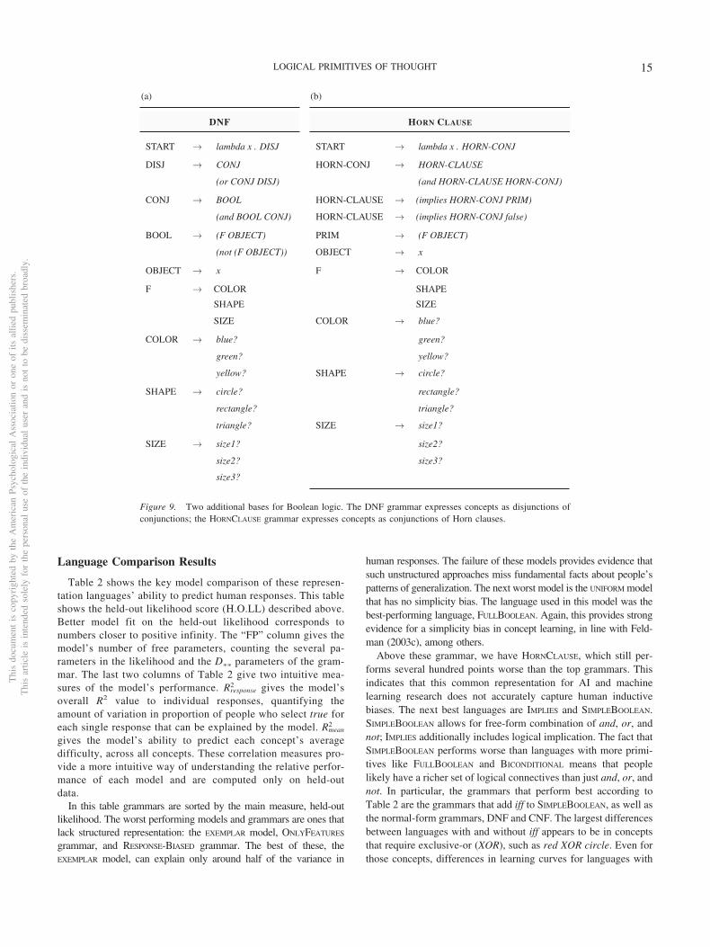
Language Comparison Results

Table 2 shows the key model comparison of these represen-tation languages’ ability to predict human responses. This tableshows the held-out likelihood score (H.O.LL) described above.Better model fit on the held-out likelihood corresponds tonumbers closer to positive infinity. The “FP” column gives themodel’s number of free parameters, counting the several pa-rameters in the likelihood and the D�� parameters of the gram-mar. The last two columns of Table 2 give two intuitive mea-sures of the model’s performance. Rresponse

2 gives the model’soverall R2 value to individual responses, quantifying theamount of variation in proportion of people who select true foreach single response that can be explained by the model. Rmean

2

gives the model’s ability to predict each concept’s averagedifficulty, across all concepts. These correlation measures pro-vide a more intuitive way of understanding the relative perfor-mance of each model and are computed only on held-outdata.

In this table grammars are sorted by the main measure, held-outlikelihood. The worst performing models and grammars are ones thatlack structured representation: the EXEMPLAR model, ONLYFEATURES

grammar, and RESPONSE-BIASED grammar. The best of these, theEXEMPLAR model, can explain only around half of the variance in

human responses. The failure of these models provides evidence thatsuch unstructured approaches miss fundamental facts about people’spatterns of generalization. The next worst model is the UNIFORM modelthat has no simplicity bias. The language used in this model was thebest-performing language, FULLBOOLEAN. Again, this provides strongevidence for a simplicity bias in concept learning, in line with Feld-man (2003c), among others.

Above these grammar, we have HORNCLAUSE, which still per-forms several hundred points worse than the top grammars. Thisindicates that this common representation for AI and machinelearning research does not accurately capture human inductivebiases. The next best languages are IMPLIES and SIMPLEBOOLEAN.SIMPLEBOOLEAN allows for free-form combination of and, or, andnot; IMPLIES additionally includes logical implication. The fact thatSIMPLEBOOLEAN performs worse than languages with more primi-tives like FULLBOOLEAN and BICONDITIONAL means that peoplelikely have a richer set of logical connectives than just and, or, andnot. In particular, the grammars that perform best according toTable 2 are the grammars that add iff to SIMPLEBOOLEAN, as well asthe normal-form grammars, DNF and CNF. The largest differencesbetween languages with and without iff appears to be in conceptsthat require exclusive-or (XOR), such as red XOR circle. Even forthose concepts, differences in learning curves for languages with

Figure 9. Two additional bases for Boolean logic. The DNF grammar expresses concepts as disjunctions ofconjunctions; the HORNCLAUSE grammar expresses concepts as conjunctions of Horn clauses.

Thi

sdo

cum

ent

isco

pyri

ghte

dby

the

Am

eric

anPs

ycho

logi

cal

Ass

ocia

tion

oron

eof

itsal

lied

publ

ishe

rs.

Thi

sar

ticle

isin

tend

edso

lely

for

the

pers

onal

use

ofth

ein

divi

dual

user

and

isno

tto

bedi

ssem

inat

edbr

oadl

y.


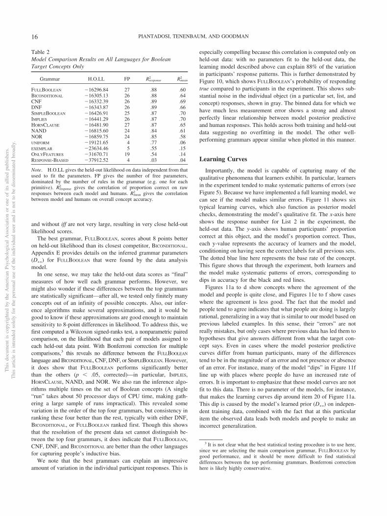
and without iff are not very large, resulting in very close held-outlikelihood scores.

The best grammar, FULLBOOLEAN, scores about 8 points betteron held-out likelihood than its closest competitor, BICONDITIONAL.Appendix E provides details on the inferred grammar parameters(D��) for FULLBOOLEAN that were found by the data analysismodel.

In one sense, we may take the held-out data scores as “final”measures of how well each grammar performs. However, wemight also wonder if these differences between the top grammarsare statistically significant—after all, we tested only finitely manyconcepts out of an infinity of possible concepts. Also, our infer-ence algorithms make several approximations, and it would begood to know if these approximations are good enough to maintainsensitivity to 8-point differences in likelihood. To address this, wefirst computed a Wilcoxon signed-ranks test, a nonparametric pairedcomparison, on the likelihood that each pair of models assigned toeach held-out data point. With Bonferroni correction for multiplecomparisons,3 this reveals no difference between the FULLBOOLEAN

language and BICONDITIONAL, CNF, DNF, or SIMPLEBOOLEAN. However,it does show that FULLBOOLEAN performs significantly betterthan the others (p .05, corrected)—in particular, IMPLIES,HORNCLAUSE, NAND, and NOR. We also ran the inference algo-rithms multiple times on the set of Boolean concepts (A single“run” takes about 50 processor days of CPU time, making gath-ering a large sample of runs impractical). This revealed somevariation in the order of the top four grammars, but consistency inranking these four better than the rest, typically with either DNF,BICONDITIONAL, or FULLBOOLEAN ranked first. Though this showsthat the resolution of the present data set cannot distinguish be-tween the top four grammars, it does indicate that FULLBOOLEAN,CNF, DNF, and BICONDITIONAL are better than the other languagesfor capturing people’s inductive bias.

We note that the best grammars can explain an impressiveamount of variation in the individual participant responses. This is

especially compelling because this correlation is computed only onheld-out data: with no parameters fit to the held-out data, thelearning model described above can explain 88% of the variationin participants’ response patterns. This is further demonstrated byFigure 10, which shows FULLBOOLEAN’s probability of respondingtrue compared to participants in the experiment. This shows sub-stantial noise in the individual object (in a particular set, list, andconcept) responses, shown in gray. The binned data for which wehave much less measurement error shows a strong and almostperfectly linear relationship between model posterior predictiveand human responses. This holds across both training and held-outdata suggesting no overfitting in the model. The other well-performing grammars appear similar when plotted in this manner.

Learning Curves

Importantly, the model is capable of capturing many of thequalitative phenomena that learners exhibit. In particular, learnersin the experiment tended to make systematic patterns of errors (seeFigure 5). Because we have implemented a full learning model, wecan see if the model makes similar errors. Figure 11 shows sixtypical learning curves, which also function as posterior modelchecks, demonstrating the model’s qualitative fit. The x-axis hereshows the response number for List 2 in the experiment, theheld-out data. The y-axis shows human participants’ proportioncorrect at this object, and the model’s proportion correct. Thus,each y-value represents the accuracy of learners and the model,conditioning on having seen the correct labels for all previous sets.The dotted blue line here represents the base rate of the concept.This figure shows that through the experiment, both learners andthe model make systematic patterns of errors, corresponding todips in accuracy for the black and red lines.

Figures 11a to d show concepts where the agreement of themodel and people is quite close, and Figures 11e to f show caseswhere the agreement is less good. The fact that the model andpeople tend to agree indicates that what people are doing is largelyrational, generalizing in a way that is similar to our model based onprevious labeled examples. In this sense, their “errors” are notreally mistakes, but only cases where previous data has led them tohypotheses that give answers different from what the target con-cept says. Even in cases where the model posterior predictivecurves differ from human participants, many of the differencestend to be in the magnitude of an error and not presence or absenceof an error. For instance, many of the model “dips” in Figure 11fline up with places where people do have an increased rate oferrors. It is important to emphasize that these model curves are notfit to this data. There is no parameter of the models, for instance,that makes the learning curves dip around item 20 of Figure 11a.This dip is caused by the model’s learned prior (D��) on indepen-dent training data, combined with the fact that at this particularitem the observed data leads both models and people to make anincorrect generalization.

3 It is not clear what the best statistical testing procedure is to use here,since we are selecting the main comparison grammar, FULLBOOLEAN bygood performance, and it should be more difficult to find statisticaldifferences between the top performing grammars. Bonferroni correctionhere is likely highly conservative.

Table 2Model Comparison Results on All Languages for BooleanTarget Concepts Only

Grammar H.O.LL FP Rresponse2 Rmean

2

FULLBOOLEAN �16296.84 27 .88 .60BICONDITIONAL �16305.13 26 .88 .64CNF �16332.39 26 .89 .69DNF �16343.87 26 .89 .66SIMPLEBOOLEAN �16426.91 25 .87 .70IMPLIES �16441.29 26 .87 .70HORNCLAUSE �16481.90 27 .87 .65NAND �16815.60 24 .84 .61NOR �16859.75 24 .85 .58UNIFORM �19121.65 4 .77 .06EXEMPLAR �23634.46 5 .55 .15ONLYFEATURES �31670.71 19 .54 .14RESPONSE-BIASED �37912.52 4 .03 .04

Note. H.O.LL gives the held-out likelihood on data independent from thatused to fit the parameters. FP gives the number of free parameters,dominated by the number of rules in the grammar (e.g. one for eachprimitive). Rresponse

2 gives the correlation of proportion correct on rawresponses between each model and humans. Rmean

2 gives the correlationbetween model and humans on overall concept accuracy.

Thi

sdo

cum

ent

isco

pyri

ghte

dby

the

Am

eric

anPs

ycho

logi

cal

Ass

ocia

tion

oron

eof

itsal

lied

publ

ishe

rs.

Thi

sar

ticle

isin

tend

edso

lely

for

the

pers

onal

use

ofth

ein

divi

dual

user

and

isno

tto

bedi

ssem

inat

edbr

oadl

y.


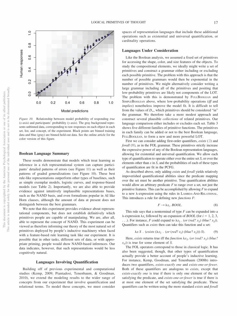
Boolean Language Summary

These results demonstrate that models which treat learning asinference in a rich representational system can capture partici-pants’ detailed patterns of errors (see Figure 11) as well as theirpatterns of graded generalizations (see Figure 10). These bestrule-like representations outperform other types of baselines, suchas simple exemplar models, logistic curves, and response-biasedmodels (see Table 2). Importantly, we are also able to provideevidence against intuitively implausible representations bases,such as the NAND basis, and even formalisms popular in AI likeHorn clauses, although the amount of data at present does notdistinguish between the best grammars.

We note that this experiment provides evidence about represen-tational components, but does not establish definitively whichprimitives people are capable of manipulating. We are, after all,able to represent the concept of NAND. This experiment can beviewed as therefore informing our theory of the most natural set ofprimitives deployed by people’s inductive machinery when facedwith a feature-based rule learning task like our experiment. It ispossible that in other tasks, different sets of data, or with appro-priate priming, people would show NAND-based inferences. Ourdata indicates, however, that such representations would be lesscognitively natural.

Languages Involving Quantification

Building off of previous experimental and computationalstudies (Kemp, 2009; Piantadosi, Tenenbaum, & Goodman,2010), we extend the modeling results to the wider range ofconcepts from our experiment that involve quantification andrelational terms. To model these concepts, we must consider

spaces of representation languages that include these additionaloperations such as existential and universal quantification, orcardinality operations.

Languages Under Consideration

Like the Boolean analysis, we assumed a fixed set of primitivesfor accessing the shape, color, and size features of the objects. Tostudy the compositional elements, we ideally might write a set ofprimitives and construct a grammar either including or excludingeach possible primitive. The problem with this approach is that thenumber of possible grammars would then be exponential in thenumber of primitives. We might alternatively consider writing alarge grammar including all of the primitives and positing thatlow-probability primitives are likely not components of the LOT.The problem with this is demonstrated by FULLBOOLEAN andSIMPLEBOOLEAN above, where low-probability operations (iff andimplies) nonetheless improve the model fit. It is difficult to tellfrom the values of D�� which primitives should be considered “in”the grammar. We therefore take a more modest approach andconstruct several plausible collections of related primitives. Ourlanguage comparison either includes or excludes each set. Table 3shows five different families of primitive functions. The primitivesin each family can be added or not to the best Boolean language,FULLBOOLEAN, to form a new and more powerful LOT.

First we can consider adding first-order quantifiers, exists (?) andforall (@), as in the FOL grammar. These primitives strictly increasethe expressive power of any of the Boolean representation languages,allowing for existential and universal quantification. We allow eachtype of quantification to operate either over the entire set S, or over theelements other than x in S, and the probabilities of each of these typesof quantification are fit in the PCFG.

As described above, only adding exists and forall yields relativelyimpoverished quantificational abilities since the predicate mappingover the set must be another primitive. True quantification abilitieswould allow an arbitrary predicate F to range over a set, not just theprimitive features. This can be accomplished by allowing F to expandto a new �-expression using the rules in LAMBDA-AND-RELATIONAL.This introduces a rule for defining new functions F:

F ¡ �xi . BOOL. (8)

This rule says that a nonterminal of type F can be expanded into a�-expression �xi followed by an expansion of BOOL (for i � 1, 2, 3,. . .). For instance, F could expand to �x2 . (or (red? x2) (blue? x2)).Quantifiers such as exists then can take this function and a set:

�x S . (exists (�x2 . (or (red? x2) (blue? x2))) S). (9)

Here, exists returns true iff the function �x2. (or (red? x2) (blue?x2)) is true for some element of S.

The FOL operators correspond to those in classical logic. It hasalso been suggested, though, that other types of quantificationactually provide a better account of people’s inductive learning.For instance, Kemp, Goodman, and Tenenbaum (2008b) intro-duces two quantifiers, exists-exactly one and exists-one-or-fewer.Both of these quantifiers are analogous to exists, except thatexists-exactly one is true if there is only one element of the setsatisfying the predicate, and exists-one-or-fewer is true if there isat most one element of the set satisfying the predicate. Thesequantifiers can be written using the more standard exists and forall

Figure 10. Relationship between model probability of responding true(x-axis) and participants’ probability (y-axis). The gray background repre-sents unbinned data, corresponding to raw responses on each object in eachset, list, and concept, of the experiment. Black points are binned trainingdata and blue (gray) are binned held-out data. See the online article for thecolor version of this figure.

Thi

sdo

cum

ent

isco

pyri

ghte

dby

the

Am

eric

anPs

ycho

logi

cal

Ass

ocia

tion

oron

eof

itsal

lied

publ

ishe

rs.

Thi

sar

ticle

isin

tend

edso

lely

for

the

pers

onal

use

ofth

ein

divi

dual

user

and

isno

tto

bedi

ssem

inat

edbr

oadl

y.


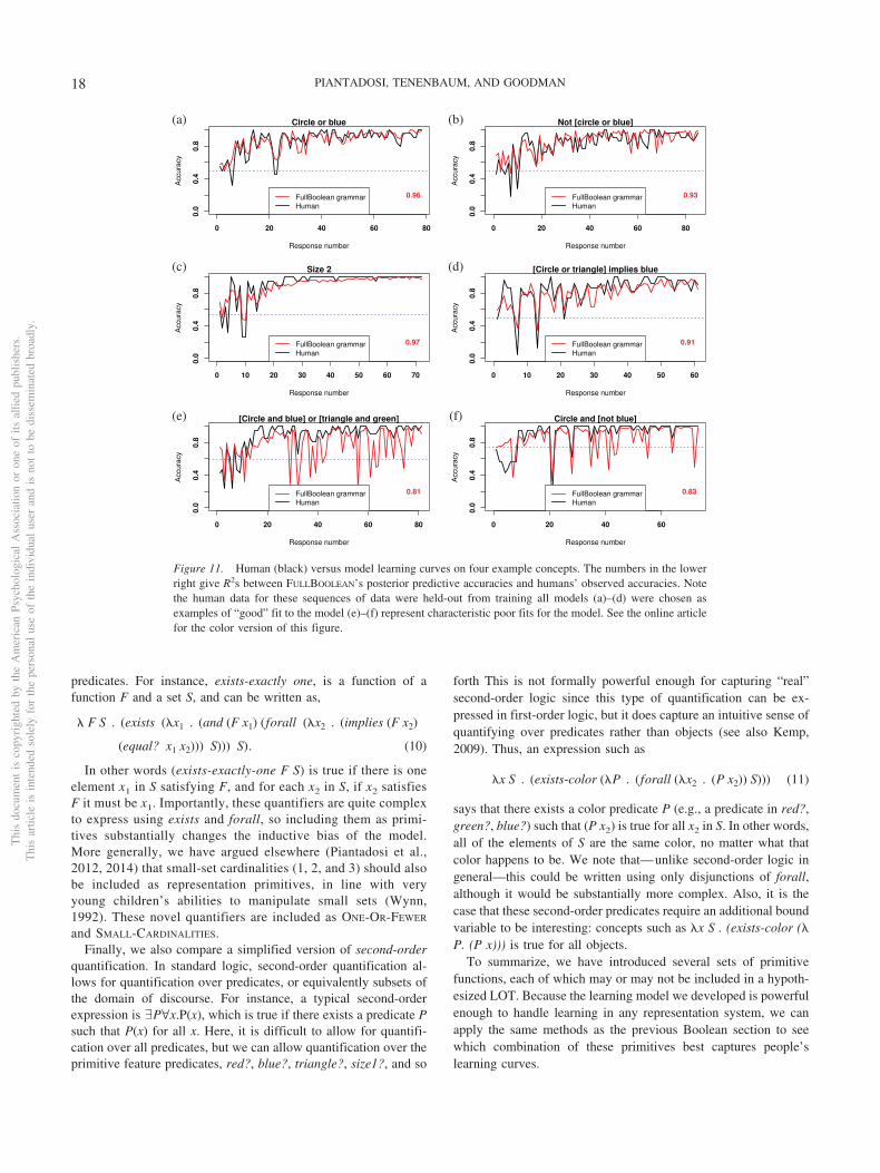
predicates. For instance, exists-exactly one, is a function of afunction F and a set S, and can be written as,

� F S . (exists (�x1 . (and (F x1) (forall (�x2 . (implies (F x2)

(equal? x1 x2))) S))) S). (10)

In other words (exists-exactly-one F S) is true if there is oneelement x1 in S satisfying F, and for each x2 in S, if x2 satisfiesF it must be x1. Importantly, these quantifiers are quite complexto express using exists and forall, so including them as primi-tives substantially changes the inductive bias of the model.More generally, we have argued elsewhere (Piantadosi et al.,2012, 2014) that small-set cardinalities (1, 2, and 3) should alsobe included as representation primitives, in line with veryyoung children’s abilities to manipulate small sets (Wynn,1992). These novel quantifiers are included as ONE-OR-FEWER

and SMALL-CARDINALITIES.Finally, we also compare a simplified version of second-order

quantification. In standard logic, second-order quantification al-lows for quantification over predicates, or equivalently subsets ofthe domain of discourse. For instance, a typical second-orderexpression is [email protected](x), which is true if there exists a predicate Psuch that P(x) for all x. Here, it is difficult to allow for quantifi-cation over all predicates, but we can allow quantification over theprimitive feature predicates, red?, blue?, triangle?, size1?, and so

forth This is not formally powerful enough for capturing “real”second-order logic since this type of quantification can be ex-pressed in first-order logic, but it does capture an intuitive sense ofquantifying over predicates rather than objects (see also Kemp,2009). Thus, an expression such as

�x S . (exists-color (�P . (forall (�x2 . (P x2)) S))) (11)

says that there exists a color predicate P (e.g., a predicate in red?,green?, blue?) such that (P x2) is true for all x2 in S. In other words,all of the elements of S are the same color, no matter what thatcolor happens to be. We note that—unlike second-order logic ingeneral—this could be written using only disjunctions of forall,although it would be substantially more complex. Also, it is thecase that these second-order predicates require an additional boundvariable to be interesting: concepts such as �x S . (exists-color (�P. (P x))) is true for all objects.

To summarize, we have introduced several sets of primitivefunctions, each of which may or may not be included in a hypoth-esized LOT. Because the learning model we developed is powerfulenough to handle learning in any representation system, we canapply the same methods as the previous Boolean section to seewhich combination of these primitives best captures people’slearning curves.

Figure 11. Human (black) versus model learning curves on four example concepts. The numbers in the lowerright give R2s between FULLBOOLEAN’s posterior predictive accuracies and humans’ observed accuracies. Notethe human data for these sequences of data were held-out from training all models (a)–(d) were chosen asexamples of “good” fit to the model (e)–(f) represent characteristic poor fits for the model. See the online articlefor the color version of this figure.

Thi

sdo

cum

ent

isco

pyri

ghte

dby

the

Am

eric

anPs

ycho

logi

cal

Ass

ocia

tion

oron

eof

itsal

lied

publ

ishe

rs.

Thi

sar

ticle

isin

tend

edso

lely

for

the

pers

onal

use

ofth

ein

divi

dual

user

and

isno

tto

bedi

ssem

inat

edbr

oadl

y.


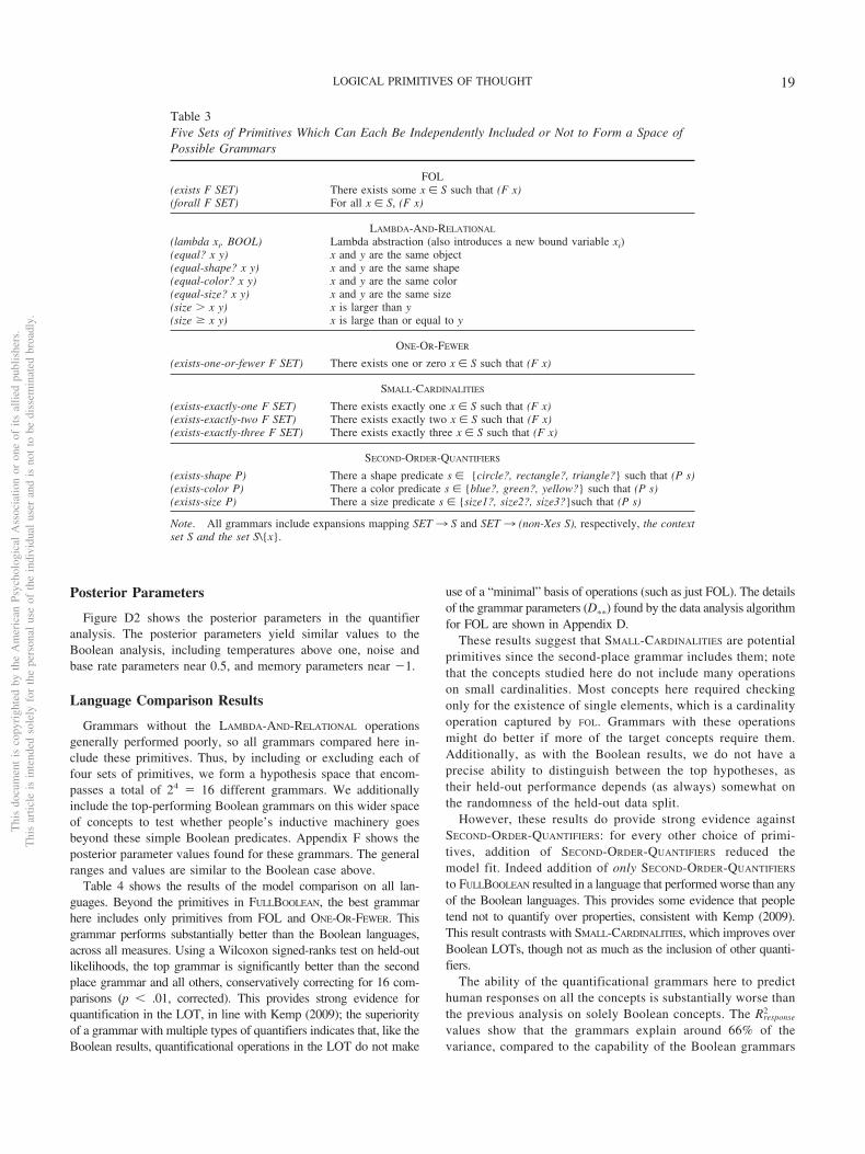
Posterior Parameters

Figure D2 shows the posterior parameters in the quantifieranalysis. The posterior parameters yield similar values to theBoolean analysis, including temperatures above one, noise andbase rate parameters near 0.5, and memory parameters near �1.

Language Comparison Results

Grammars without the LAMBDA-AND-RELATIONAL operationsgenerally performed poorly, so all grammars compared here in-clude these primitives. Thus, by including or excluding each offour sets of primitives, we form a hypothesis space that encom-passes a total of 24 � 16 different grammars. We additionallyinclude the top-performing Boolean grammars on this wider spaceof concepts to test whether people’s inductive machinery goesbeyond these simple Boolean predicates. Appendix F shows theposterior parameter values found for these grammars. The generalranges and values are similar to the Boolean case above.

Table 4 shows the results of the model comparison on all lan-guages. Beyond the primitives in FULLBOOLEAN, the best grammarhere includes only primitives from FOL and ONE-OR-FEWER. Thisgrammar performs substantially better than the Boolean languages,across all measures. Using a Wilcoxon signed-ranks test on held-outlikelihoods, the top grammar is significantly better than the secondplace grammar and all others, conservatively correcting for 16 com-parisons (p .01, corrected). This provides strong evidence forquantification in the LOT, in line with Kemp (2009); the superiorityof a grammar with multiple types of quantifiers indicates that, like theBoolean results, quantificational operations in the LOT do not make

use of a “minimal” basis of operations (such as just FOL). The detailsof the grammar parameters (D��) found by the data analysis algorithmfor FOL are shown in Appendix D.

These results suggest that SMALL-CARDINALITIES are potentialprimitives since the second-place grammar includes them; notethat the concepts studied here do not include many operationson small cardinalities. Most concepts here required checkingonly for the existence of single elements, which is a cardinalityoperation captured by FOL. Grammars with these operationsmight do better if more of the target concepts require them.Additionally, as with the Boolean results, we do not have aprecise ability to distinguish between the top hypotheses, astheir held-out performance depends (as always) somewhat onthe randomness of the held-out data split.

However, these results do provide strong evidence againstSECOND-ORDER-QUANTIFIERS: for every other choice of primi-tives, addition of SECOND-ORDER-QUANTIFIERS reduced themodel fit. Indeed addition of only SECOND-ORDER-QUANTIFIERS

to FULLBOOLEAN resulted in a language that performed worse than anyof the Boolean languages. This provides some evidence that peopletend not to quantify over properties, consistent with Kemp (2009).This result contrasts with SMALL-CARDINALITIES, which improves overBoolean LOTs, though not as much as the inclusion of other quanti-fiers.

The ability of the quantificational grammars here to predicthuman responses on all the concepts is substantially worse thanthe previous analysis on solely Boolean concepts. The Rresponse

2

values show that the grammars explain around 66% of thevariance, compared to the capability of the Boolean grammars

Table 3Five Sets of Primitives Which Can Each Be Independently Included or Not to Form a Space ofPossible Grammars

FOL(exists F SET) There exists some x � S such that (F x)(forall F SET) For all x � S, (F x)

LAMBDA-AND-RELATIONAL

(lambda xi. BOOL) Lambda abstraction (also introduces a new bound variable xi)(equal? x y) x and y are the same object(equal-shape? x y) x and y are the same shape(equal-color? x y) x and y are the same color(equal-size? x y) x and y are the same size(size � x y) x is larger than y(size � x y) x is large than or equal to y

ONE-OR-FEWER

(exists-one-or-fewer F SET) There exists one or zero x � S such that (F x)

SMALL-CARDINALITIES

(exists-exactly-one F SET) There exists exactly one x � S such that (F x)(exists-exactly-two F SET) There exists exactly two x � S such that (F x)(exists-exactly-three F SET) There exists exactly three x � S such that (F x)

SECOND-ORDER-QUANTIFIERS

(exists-shape P) There a shape predicate s � {circle?, rectangle?, triangle?} such that (P s)(exists-color P) There a color predicate s � {blue?, green?, yellow?} such that (P s)(exists-size P) There a size predicate s � {size1?, size2?, size3?}such that (P s)

Note. All grammars include expansions mapping SET ¡ S and SET ¡ (non-Xes S), respectively, the contextset S and the set S\{x}.

Thi

sdo

cum

ent

isco

pyri

ghte

dby

the

Am

eric

anPs

ycho

logi

cal

Ass

ocia

tion

oron

eof

itsal

lied

publ

ishe

rs.

Thi

sar

ticle

isin

tend

edso

lely

for

the

pers

onal

use

ofth

ein

divi

dual

user

and

isno

tto

bedi

ssem

inat

edbr

oadl

y.


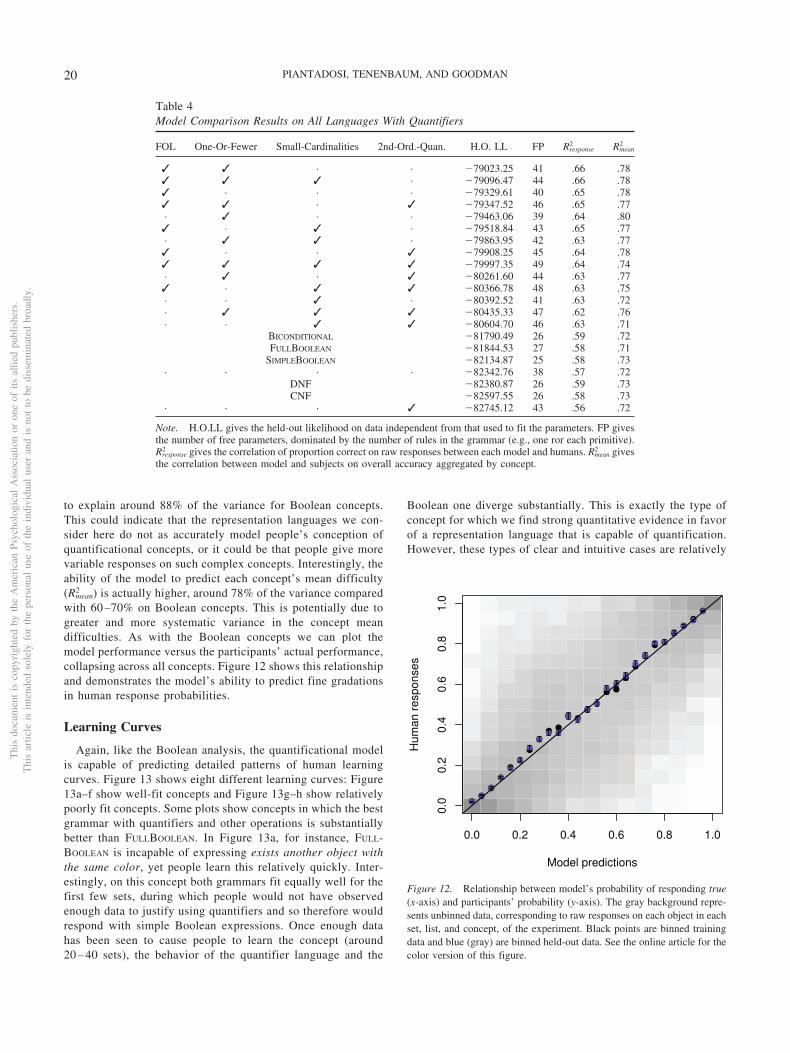
to explain around 88% of the variance for Boolean concepts.This could indicate that the representation languages we con-sider here do not as accurately model people’s conception ofquantificational concepts, or it could be that people give morevariable responses on such complex concepts. Interestingly, theability of the model to predict each concept’s mean difficulty(Rmean

2 ) is actually higher, around 78% of the variance comparedwith 60 –70% on Boolean concepts. This is potentially due togreater and more systematic variance in the concept meandifficulties. As with the Boolean concepts we can plot themodel performance versus the participants’ actual performance,collapsing across all concepts. Figure 12 shows this relationshipand demonstrates the model’s ability to predict fine gradationsin human response probabilities.

Learning Curves

Again, like the Boolean analysis, the quantificational modelis capable of predicting detailed patterns of human learningcurves. Figure 13 shows eight different learning curves: Figure13a–f show well-fit concepts and Figure 13g–h show relativelypoorly fit concepts. Some plots show concepts in which the bestgrammar with quantifiers and other operations is substantiallybetter than FULLBOOLEAN. In Figure 13a, for instance, FULL-BOOLEAN is incapable of expressing exists another object withthe same color, yet people learn this relatively quickly. Inter-estingly, on this concept both grammars fit equally well for thefirst few sets, during which people would not have observedenough data to justify using quantifiers and so therefore wouldrespond with simple Boolean expressions. Once enough datahas been seen to cause people to learn the concept (around20 – 40 sets), the behavior of the quantifier language and the

Boolean one diverge substantially. This is exactly the type ofconcept for which we find strong quantitative evidence in favorof a representation language that is capable of quantification.However, these types of clear and intuitive cases are relatively

Table 4Model Comparison Results on All Languages With Quantifiers

FOL One-Or-Fewer Small-Cardinalities 2nd-Ord.-Quan. H.O. LL FP Rresponse2 Rmean

2

✓ ✓ · · �79023.25 41 .66 .78✓ ✓ ✓ · �79096.47 44 .66 .78✓ · · · �79329.61 40 .65 .78✓ ✓ · ✓ �79347.52 46 .65 .77· ✓ · · �79463.06 39 .64 .80✓ · ✓ · �79518.84 43 .65 .77· ✓ ✓ · �79863.95 42 .63 .77✓ · · ✓ �79908.25 45 .64 .78✓ ✓ ✓ ✓ �79997.35 49 .64 .74· ✓ · ✓ �80261.60 44 .63 .77✓ · ✓ ✓ �80366.78 48 .63 .75· · ✓ · �80392.52 41 .63 .72· ✓ ✓ ✓ �80435.33 47 .62 .76· · ✓ ✓ �80604.70 46 .63 .71

BICONDITIONAL �81790.49 26 .59 .72FULLBOOLEAN �81844.53 27 .58 .71

SIMPLEBOOLEAN �82134.87 25 .58 .73· · · · �82342.76 38 .57 .72

DNF �82380.87 26 .59 .73CNF �82597.55 26 .58 .73

· · · ✓ �82745.12 43 .56 .72

Note. H.O.LL gives the held-out likelihood on data independent from that used to fit the parameters. FP givesthe number of free parameters, dominated by the number of rules in the grammar (e.g., one ror each primitive).Rresponse

2 gives the correlation of proportion correct on raw responses between each model and humans. Rmean2 gives

the correlation between model and subjects on overall accuracy aggregated by concept.

Figure 12. Relationship between model’s probability of responding true(x-axis) and participants’ probability (y-axis). The gray background repre-sents unbinned data, corresponding to raw responses on each object in eachset, list, and concept, of the experiment. Black points are binned trainingdata and blue (gray) are binned held-out data. See the online article for thecolor version of this figure.

Thi

sdo

cum

ent

isco

pyri

ghte

dby

the

Am

eric

anPs

ycho

logi

cal

Ass

ocia

tion

oron

eof

itsal

lied

publ

ishe

rs.

Thi

sar

ticle

isin

tend

edso

lely

for

the

pers

onal

use

ofth

ein

divi

dual

user

and

isno

tto

bedi

ssem

inat

edbr

oadl

y.


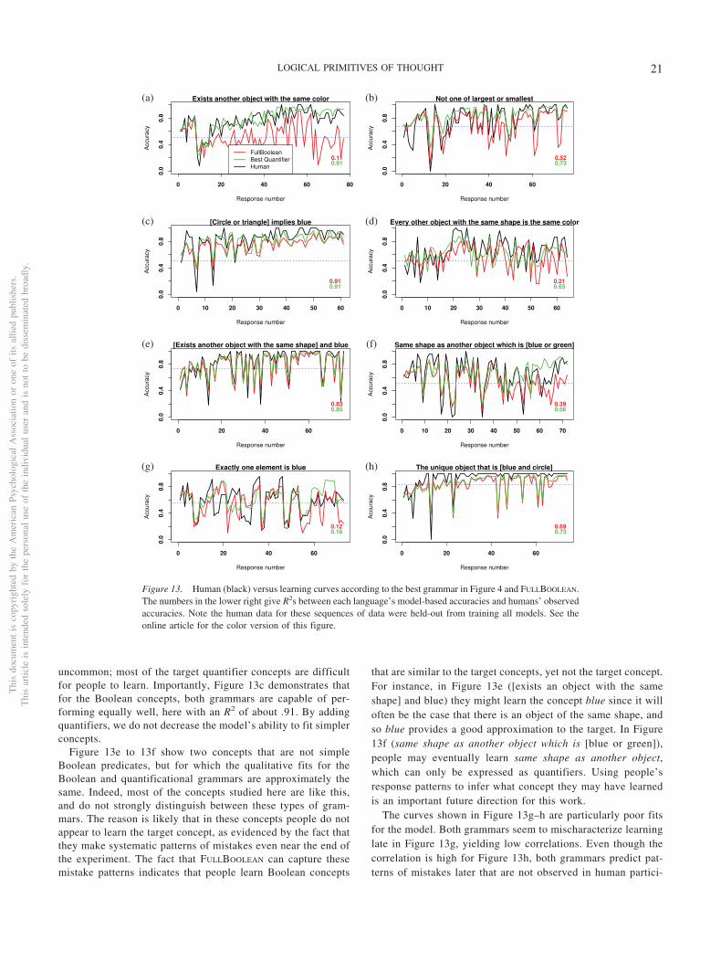
uncommon; most of the target quantifier concepts are difficultfor people to learn. Importantly, Figure 13c demonstrates thatfor the Boolean concepts, both grammars are capable of per-forming equally well, here with an R2 of about .91. By addingquantifiers, we do not decrease the model’s ability to fit simplerconcepts.

Figure 13e to 13f show two concepts that are not simpleBoolean predicates, but for which the qualitative fits for theBoolean and quantificational grammars are approximately thesame. Indeed, most of the concepts studied here are like this,and do not strongly distinguish between these types of gram-mars. The reason is likely that in these concepts people do notappear to learn the target concept, as evidenced by the fact thatthey make systematic patterns of mistakes even near the end ofthe experiment. The fact that FULLBOOLEAN can capture thesemistake patterns indicates that people learn Boolean concepts

that are similar to the target concepts, yet not the target concept.For instance, in Figure 13e ([exists an object with the sameshape] and blue) they might learn the concept blue since it willoften be the case that there is an object of the same shape, andso blue provides a good approximation to the target. In Figure13f (same shape as another object which is [blue or green]),people may eventually learn same shape as another object,which can only be expressed as quantifiers. Using people’sresponse patterns to infer what concept they may have learnedis an important future direction for this work.

The curves shown in Figure 13g–h are particularly poor fitsfor the model. Both grammars seem to mischaracterize learninglate in Figure 13g, yielding low correlations. Even though thecorrelation is high for Figure 13h, both grammars predict pat-terns of mistakes later that are not observed in human partici-

Figure 13. Human (black) versus learning curves according to the best grammar in Figure 4 and FULLBOOLEAN.The numbers in the lower right give R2s between each language’s model-based accuracies and humans’ observedaccuracies. Note the human data for these sequences of data were held-out from training all models. See theonline article for the color version of this figure.

Thi

sdo

cum

ent

isco

pyri

ghte

dby

the

Am

eric

anPs

ycho

logi

cal

Ass

ocia

tion

oron

eof

itsal

lied

publ

ishe

rs.

Thi

sar

ticle

isin

tend

edso

lely

for

the

pers

onal

use

ofth

ein

divi

dual

user

and

isno

tto

bedi

ssem

inat

edbr

oadl

y.


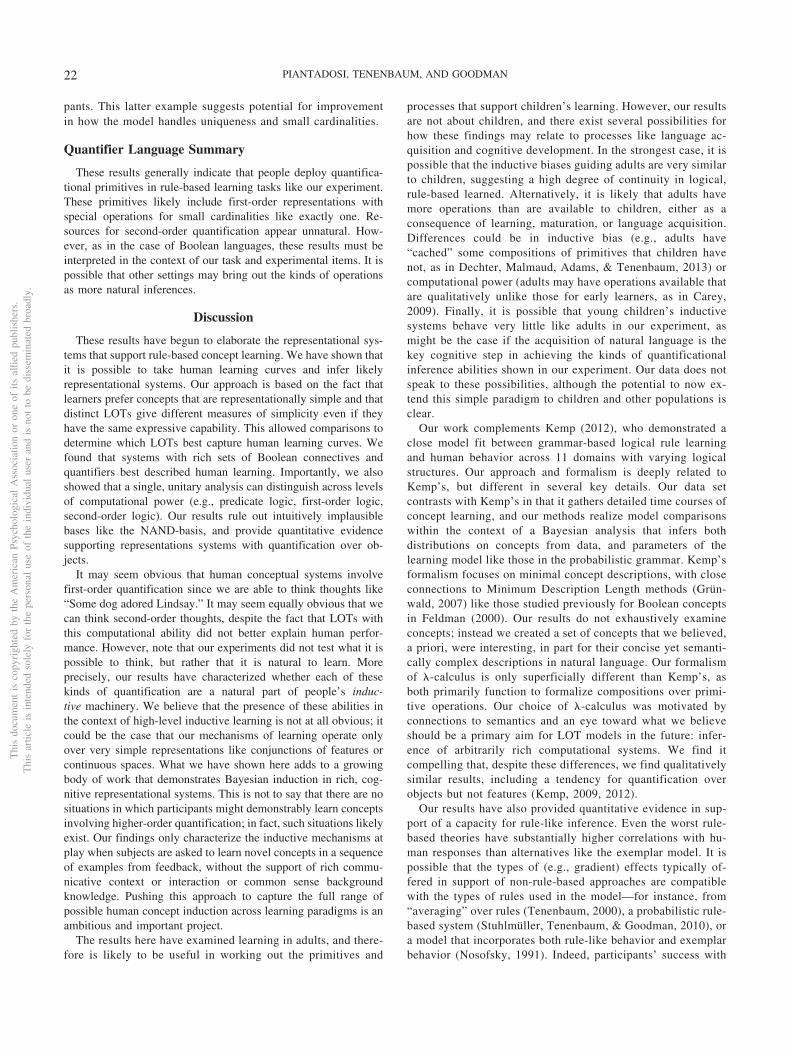
pants. This latter example suggests potential for improvementin how the model handles uniqueness and small cardinalities.

Quantifier Language Summary

These results generally indicate that people deploy quantifica-tional primitives in rule-based learning tasks like our experiment.These primitives likely include first-order representations withspecial operations for small cardinalities like exactly one. Re-sources for second-order quantification appear unnatural. How-ever, as in the case of Boolean languages, these results must beinterpreted in the context of our task and experimental items. It ispossible that other settings may bring out the kinds of operationsas more natural inferences.

Discussion

These results have begun to elaborate the representational sys-tems that support rule-based concept learning. We have shown thatit is possible to take human learning curves and infer likelyrepresentational systems. Our approach is based on the fact thatlearners prefer concepts that are representationally simple and thatdistinct LOTs give different measures of simplicity even if theyhave the same expressive capability. This allowed comparisons todetermine which LOTs best capture human learning curves. Wefound that systems with rich sets of Boolean connectives andquantifiers best described human learning. Importantly, we alsoshowed that a single, unitary analysis can distinguish across levelsof computational power (e.g., predicate logic, first-order logic,second-order logic). Our results rule out intuitively implausiblebases like the NAND-basis, and provide quantitative evidencesupporting representations systems with quantification over ob-jects.

It may seem obvious that human conceptual systems involvefirst-order quantification since we are able to think thoughts like“Some dog adored Lindsay.” It may seem equally obvious that wecan think second-order thoughts, despite the fact that LOTs withthis computational ability did not better explain human perfor-mance. However, note that our experiments did not test what it ispossible to think, but rather that it is natural to learn. Moreprecisely, our results have characterized whether each of thesekinds of quantification are a natural part of people’s induc-tive machinery. We believe that the presence of these abilities inthe context of high-level inductive learning is not at all obvious; itcould be the case that our mechanisms of learning operate onlyover very simple representations like conjunctions of features orcontinuous spaces. What we have shown here adds to a growingbody of work that demonstrates Bayesian induction in rich, cog-nitive representational systems. This is not to say that there are nosituations in which participants might demonstrably learn conceptsinvolving higher-order quantification; in fact, such situations likelyexist. Our findings only characterize the inductive mechanisms atplay when subjects are asked to learn novel concepts in a sequenceof examples from feedback, without the support of rich commu-nicative context or interaction or common sense backgroundknowledge. Pushing this approach to capture the full range ofpossible human concept induction across learning paradigms is anambitious and important project.

The results here have examined learning in adults, and there-fore is likely to be useful in working out the primitives and

processes that support children’s learning. However, our resultsare not about children, and there exist several possibilities forhow these findings may relate to processes like language ac-quisition and cognitive development. In the strongest case, it ispossible that the inductive biases guiding adults are very similarto children, suggesting a high degree of continuity in logical,rule-based learned. Alternatively, it is likely that adults havemore operations than are available to children, either as aconsequence of learning, maturation, or language acquisition.Differences could be in inductive bias (e.g., adults have“cached” some compositions of primitives that children havenot, as in Dechter, Malmaud, Adams, & Tenenbaum, 2013) orcomputational power (adults may have operations available thatare qualitatively unlike those for early learners, as in Carey,2009). Finally, it is possible that young children’s inductivesystems behave very little like adults in our experiment, asmight be the case if the acquisition of natural language is thekey cognitive step in achieving the kinds of quantificationalinference abilities shown in our experiment. Our data does notspeak to these possibilities, although the potential to now ex-tend this simple paradigm to children and other populations isclear.

Our work complements Kemp (2012), who demonstrated aclose model fit between grammar-based logical rule learningand human behavior across 11 domains with varying logicalstructures. Our approach and formalism is deeply related toKemp’s, but different in several key details. Our data setcontrasts with Kemp’s in that it gathers detailed time courses ofconcept learning, and our methods realize model comparisonswithin the context of a Bayesian analysis that infers bothdistributions on concepts from data, and parameters of thelearning model like those in the probabilistic grammar. Kemp’sformalism focuses on minimal concept descriptions, with closeconnections to Minimum Description Length methods (Grün-wald, 2007) like those studied previously for Boolean conceptsin Feldman (2000). Our results do not exhaustively examineconcepts; instead we created a set of concepts that we believed,a priori, were interesting, in part for their concise yet semanti-cally complex descriptions in natural language. Our formalismof �-calculus is only superficially different than Kemp’s, asboth primarily function to formalize compositions over primi-tive operations. Our choice of �-calculus was motivated byconnections to semantics and an eye toward what we believeshould be a primary aim for LOT models in the future: infer-ence of arbitrarily rich computational systems. We find itcompelling that, despite these differences, we find qualitativelysimilar results, including a tendency for quantification overobjects but not features (Kemp, 2009, 2012).

Our results have also provided quantitative evidence in sup-port of a capacity for rule-like inference. Even the worst rule-based theories have substantially higher correlations with hu-man responses than alternatives like the exemplar model. It ispossible that the types of (e.g., gradient) effects typically of-fered in support of non-rule-based approaches are compatiblewith the types of rules used in the model—for instance, from“averaging” over rules (Tenenbaum, 2000), a probabilistic rule-based system (Stuhlmüller, Tenenbaum, & Goodman, 2010), ora model that incorporates both rule-like behavior and exemplarbehavior (Nosofsky, 1991). Indeed, participants’ success with

Thi

sdo

cum

ent

isco

pyri

ghte

dby

the

Am

eric

anPs

ycho

logi

cal

Ass

ocia

tion

oron

eof

itsal

lied

publ

ishe

rs.

Thi

sar

ticle

isin

tend

edso

lely

for

the

pers

onal

use

ofth

ein

divi

dual

user

and

isno

tto

bedi

ssem

inat

edbr

oadl

y.


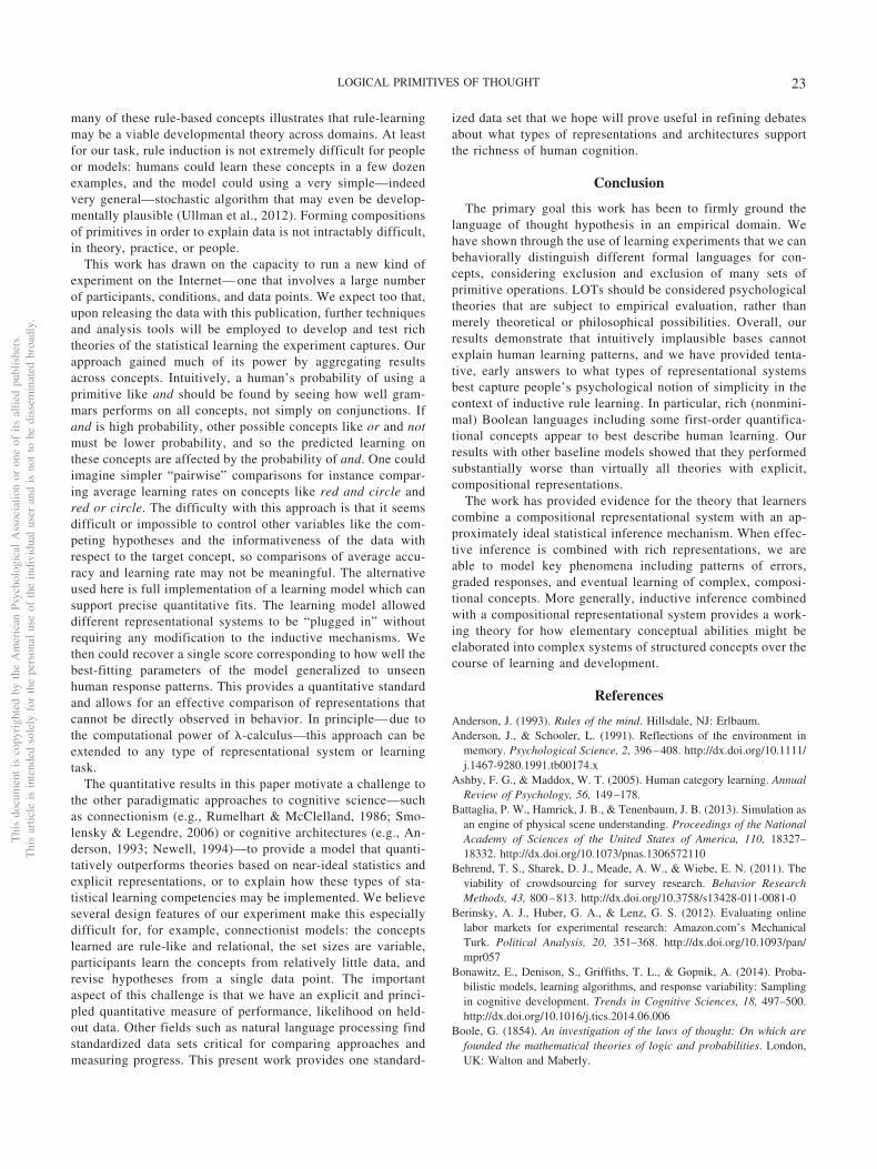
many of these rule-based concepts illustrates that rule-learningmay be a viable developmental theory across domains. At leastfor our task, rule induction is not extremely difficult for peopleor models: humans could learn these concepts in a few dozenexamples, and the model could using a very simple—indeedvery general—stochastic algorithm that may even be develop-mentally plausible (Ullman et al., 2012). Forming compositionsof primitives in order to explain data is not intractably difficult,in theory, practice, or people.

This work has drawn on the capacity to run a new kind ofexperiment on the Internet— one that involves a large numberof participants, conditions, and data points. We expect too that,upon releasing the data with this publication, further techniquesand analysis tools will be employed to develop and test richtheories of the statistical learning the experiment captures. Ourapproach gained much of its power by aggregating resultsacross concepts. Intuitively, a human’s probability of using aprimitive like and should be found by seeing how well gram-mars performs on all concepts, not simply on conjunctions. Ifand is high probability, other possible concepts like or and notmust be lower probability, and so the predicted learning onthese concepts are affected by the probability of and. One couldimagine simpler “pairwise” comparisons for instance compar-ing average learning rates on concepts like red and circle andred or circle. The difficulty with this approach is that it seemsdifficult or impossible to control other variables like the com-peting hypotheses and the informativeness of the data withrespect to the target concept, so comparisons of average accu-racy and learning rate may not be meaningful. The alternativeused here is full implementation of a learning model which cansupport precise quantitative fits. The learning model alloweddifferent representational systems to be “plugged in” withoutrequiring any modification to the inductive mechanisms. Wethen could recover a single score corresponding to how well thebest-fitting parameters of the model generalized to unseenhuman response patterns. This provides a quantitative standardand allows for an effective comparison of representations thatcannot be directly observed in behavior. In principle— due tothe computational power of �-calculus—this approach can beextended to any type of representational system or learningtask.

The quantitative results in this paper motivate a challenge tothe other paradigmatic approaches to cognitive science—suchas connectionism (e.g., Rumelhart & McClelland, 1986; Smo-lensky & Legendre, 2006) or cognitive architectures (e.g., An-derson, 1993; Newell, 1994)—to provide a model that quanti-tatively outperforms theories based on near-ideal statistics andexplicit representations, or to explain how these types of sta-tistical learning competencies may be implemented. We believeseveral design features of our experiment make this especiallydifficult for, for example, connectionist models: the conceptslearned are rule-like and relational, the set sizes are variable,participants learn the concepts from relatively little data, andrevise hypotheses from a single data point. The importantaspect of this challenge is that we have an explicit and princi-pled quantitative measure of performance, likelihood on held-out data. Other fields such as natural language processing findstandardized data sets critical for comparing approaches andmeasuring progress. This present work provides one standard-

ized data set that we hope will prove useful in refining debatesabout what types of representations and architectures supportthe richness of human cognition.

Conclusion

The primary goal this work has been to firmly ground thelanguage of thought hypothesis in an empirical domain. Wehave shown through the use of learning experiments that we canbehaviorally distinguish different formal languages for con-cepts, considering exclusion and exclusion of many sets ofprimitive operations. LOTs should be considered psychologicaltheories that are subject to empirical evaluation, rather thanmerely theoretical or philosophical possibilities. Overall, ourresults demonstrate that intuitively implausible bases cannotexplain human learning patterns, and we have provided tenta-tive, early answers to what types of representational systemsbest capture people’s psychological notion of simplicity in thecontext of inductive rule learning. In particular, rich (nonmini-mal) Boolean languages including some first-order quantifica-tional concepts appear to best describe human learning. Ourresults with other baseline models showed that they performedsubstantially worse than virtually all theories with explicit,compositional representations.

The work has provided evidence for the theory that learnerscombine a compositional representational system with an ap-proximately ideal statistical inference mechanism. When effec-tive inference is combined with rich representations, we areable to model key phenomena including patterns of errors,graded responses, and eventual learning of complex, composi-tional concepts. More generally, inductive inference combinedwith a compositional representational system provides a work-ing theory for how elementary conceptual abilities might beelaborated into complex systems of structured concepts over thecourse of learning and development.

References

Anderson, J. (1993). Rules of the mind. Hillsdale, NJ: Erlbaum.Anderson, J., & Schooler, L. (1991). Reflections of the environment in

memory. Psychological Science, 2, 396–408. http://dx.doi.org/10.1111/j.1467-9280.1991.tb00174.x

Ashby, F. G., & Maddox, W. T. (2005). Human category learning. AnnualReview of Psychology, 56, 149–178.

Battaglia, P. W., Hamrick, J. B., & Tenenbaum, J. B. (2013). Simulation asan engine of physical scene understanding. Proceedings of the NationalAcademy of Sciences of the United States of America, 110, 18327–18332. http://dx.doi.org/10.1073/pnas.1306572110

Behrend, T. S., Sharek, D. J., Meade, A. W., & Wiebe, E. N. (2011). Theviability of crowdsourcing for survey research. Behavior ResearchMethods, 43, 800–813. http://dx.doi.org/10.3758/s13428-011-0081-0

Berinsky, A. J., Huber, G. A., & Lenz, G. S. (2012). Evaluating onlinelabor markets for experimental research: Amazon.com’s MechanicalTurk. Political Analysis, 20, 351–368. http://dx.doi.org/10.1093/pan/mpr057

Bonawitz, E., Denison, S., Griffiths, T. L., & Gopnik, A. (2014). Proba-bilistic models, learning algorithms, and response variability: Samplingin cognitive development. Trends in Cognitive Sciences, 18, 497–500.http://dx.doi.org/10.1016/j.tics.2014.06.006

Boole, G. (1854). An investigation of the laws of thought: On which arefounded the mathematical theories of logic and probabilities. London,UK: Walton and Maberly.

Thi

sdo

cum

ent

isco

pyri

ghte

dby

the

Am

eric

anPs

ycho

logi

cal

Ass

ocia

tion

oron

eof

itsal

lied

publ

ishe

rs.

Thi

sar

ticle

isin

tend

edso

lely

for

the

pers

onal

use

ofth

ein

divi

dual

user

and

isno

tto

bedi

ssem

inat

edbr

oadl

y.


Bourne, L. (1966). Human conceptual behavior. Boston, MA: Allyn &Bacon.

Bruner, J., Goodnow, J., & Austin, G. (1956). A study of thinking. NewBrunswick, NJ: Transaction Publishers.

Carey, S. (2009). The origin of concepts. New York, NY: Oxford Univer-sity Press.

Chater, N., & Vitányi, P. (2003). Simplicity: A unifying principle incognitive science? Trends in Cognitive Sciences, 7, 19–22.

Chen, M., & Shao, Q. (1999). Monte Carlo estimation of Bayesian credibleand HPD intervals. Journal of Computational and Graphical Statistics,8, 69–92.

Church, A. (1936). An unsolvable problem of elementary number theory.American Journal of Mathematics, 58, 345–363.

Conklin, D., & Witten, I. (1994). Complexity-based induction. MachineLearning, 16, 203–225.

Dechter, E., Malmaud, J., Adams, R. P., & Tenenbaum, J. B. (2013).Bootstrap learning via modular concept discovery. In Proceedings of the23rd International Joint Conference on Artificial Intelligence (pp. 1302–1309). Palo Alto, CA: AAAI Press.

Denison, S., Bonawitz, E., Gopnik, A., & Griffiths, T. L. (2013). Rationalvariability in children’s causal inferences: The sampling hypothesis.Cognition, 126, 285–300. http://dx.doi.org/10.1016/j.cognition.2012.10.010

Domingos, P., & Richardson, M. (2007). Markov logic: A unifying frame-work for statistical relational learning. In L. Geetor & B. Taskar (Eds.),Introduction to Statistical Relational Learning (pp. 339–371). Cam-bridge, MA: MIT Press.

Dowling, W., & Gallier, J. (1984). Linear-time algorithms for testing thesatisfiability of propositional Horn formulae. The Journal of LogicProgramming, 1, 267–284.

Feldman, J. (2000). Minimization of Boolean complexity in human conceptlearning. Nature, 407, 630–633. http://dx.doi.org/10.1038/35036586

Feldman, J. (2003a). A catalog of Boolean concepts. Journal of Mathe-matical Psychology, 47, 75–89.

Feldman, J. (2003b). Simplicity and complexity in human concept learn-ing. The General Psychologist, 38, 9–15.

Feldman, J. (2003c). The simplicity principle in human concept learning.Current Directions in Psychological Science, 12, 227–232.

Fodor, J. (1975). The language of thought. Cambridge, MA: HarvardUniversity Press.

Fodor, J. (2008). LOT 2: The language of thought revisited. New York,NY: Oxford University Press.

Fodor, J., & Pylyshyn, Z. (1988). Connectionism and cognitive architec-ture: A critical analysis. In S. Pinker & J. Mehler (eds.), Connections andsymbols: Cognition special issue, pp. 3–71. Cambridge, MA: MIT Press.

Gelman, A., Carlin, J. B., Stern, H. S., & Rubin, D. B. (2014). Bayesiandata analysis (Vol. 2). Boca Raton, FL: CRC Press.

Gentner, D. (1983). Structure-mapping: A theoretical framework for anal-ogy. Cognitive Science, 7, 155–170.

Gluck, M. A., Shohamy, D., & Myers, C. (2002). How do people solve the“weather prediction” task?: Individual variability in strategies for prob-abilistic category learning. Learning & Memory, 9, 408–418.

Goodman, N. (1955). Fact, fiction and forecast. Cambridge, MA: HarvardUniversity Press.

Goodman, N., Mansinghka, V., Roy, D., Bonawitz, K., & Tenenbaum, J.(2008). Church: A language for generative models. In S. McAllester &P. Myllymaki (Eds.), Proceedings of the 24th Conference on Uncer-tainty in Artificial Intelligence (pp. 220–229). Corvallis, OR: AUAIPress.

Goodman, N., Tenenbaum, J., Feldman, J., & Griffiths, T. (2008). Arational analysis of rule-based concept learning. Cognitive Science, 32,108–154.

Goodman, N., Tenenbaum, J., & Gerstenberg, T. (2015). Concepts in a

probabilistic language of thought. In E. Margolis & S. Laurence (Eds.),The conceptual mind: New directions in the study of concepts (pp.623–655). Cambridge, MA: MIT Press.

Griffiths, T. L., & Tenenbaum, J. B. (2006). Optimal predictions ineveryday cognition. Psychological Science, 17, 767–773.

Grünwald, P. D. (2007). The minimum description length principle. Cam-bridge, MA: MIT Press.

Hackl, M. (2009). On the grammar and processing of proportional quan-tifiers: Most versus more than half. Natural Language Semantics, 17,63–98. http://dx.doi.org/10.1007/s11050-008-9039-x

Hahn, U., & Chater, N. (1998). Similarity and rules: Distinct? Exhaustive?Empirically distinguishable? Cognition, 65, 197–230.

Hampton, J. A. (1998). Similarity-based categorization and fuzziness ofnatural categories. Cognition, 65, 137–165.

Hampton, J. A. (2006). Concepts as prototypes. Psychology of Learningand Motivation, 46, 79–113.

Hastings, W. (1970). Monte Carlo sampling methods using Markov chainsand their applications. Biometrika, 57, 97–109.

Haygood, R. (1963). Rule and attribute learning as aspects of conceptualbehavior (Unpublished doctoral dissertation). University of Utah, SaltLake City, UT.

Hemmer, P., Tauber, S., & Steyvers, M. (2014). Moving beyond qualitativeevaluations of Bayesian models of cognition. Psychonomic Bulletin &Review, 22, 614–628. http://dx.doi.org/10.3758/s13423-014-0725-z

Hindley, J., & Seldin, J. (1986). Introduction to combinators and �-cal-culus. Cambridge, UK: Press Syndicate of the University of Cambridge.

Hodges, W. (1993). Logical features of Horn clauses. Handbook of Logicin Artificial Intelligence and Logic Programming, Logical Foundations,1, 449–503.

Horn, A. (1951). On sentences which are true of direct unions of algebras.Journal of Symbolic Logic, 16, 14–21.

Huszár, F., Noppeney, U., & Lengyel, M. (2010). Mind reading by ma-chine learning: A doubly Bayesian method for inferring mental repre-sentations. In Cognition in flux (pp. 2810–2815). Austin, TX: CognitiveScience Society.

Johnson, M., Griffiths, T., & Goldwater, S. (April, 2007). Bayesian infer-ence for PCFGs via Markov chain Monte Carlo. In Proceedings of theNorth American Conference on Computational Linguistics (pp. 139–146). Rochester, NY: Association for Computational Linguistics.

Katz, Y., Goodman, N., Kersting, K., Kemp, C., & Tenenbaum, J. (2008).Modeling semantic cognition as logical dimensionality reduction. InProceedings of 30th Annual Meeting of the Cognitive Science Society.Austin, TX: Cognitive Science Society.

Kemp, C. (2009). Quantification and the language of thought. In Y.Bengio, D. Schuurmans, J. D. Lafferty, C. K. I. Williams, & A. Cullotta(Eds.), Advances in neural information processing systems, 22. Re-trieved from http://papers.nips.cc/paper/3816-quantification-and-the-language-of-thought.pdf

Kemp, C. (2012). Exploring the conceptual universe. Psychological Re-view, 119, 685–722.

Kemp, C., Goodman, N., & Tenenbaum, J. (2008a). Learning and usingrelational theories. Advances in Neural Information Processing Systems,20, 753–760.

Kemp, C., Goodman, N., & Tenenbaum, J. (2008b). Theory acquisition andthe language of thought. In Proceedings of 30th Annual Meeting of theCognitive Science Society. Austin, TX: Cognitive Science Society.

Kruschke, J. (2010a). Doing Bayesian data analysis, 2nd ed.: A tutorialintroduction with R, JAGS, and Stan. San Diego, CA: Academic Press.

Kruschke, J. K. (2010b). What to believe: Bayesian methods for dataanalysis. Trends in Cognitive Sciences, 14, 293–300.

Lee, M. D. (2011). In praise of ecumenical bayes. Behavioral and BrainSciences, 34, 206–207.

Thi

sdo

cum

ent

isco

pyri

ghte

dby

the

Am

eric

anPs

ycho

logi

cal

Ass

ocia

tion

oron

eof

itsal

lied

publ

ishe

rs.

Thi

sar

ticle

isin

tend

edso

lely

for

the

pers

onal

use

ofth

ein

divi

dual

user

and

isno

tto

bedi

ssem

inat

edbr

oadl

y.


Lee, M., & Sarnecka, B. (2010). A model of knower-level behavior innumber concept development. Cognitive Science, 34, 51–67. http://dx.doi.org/10.1111/j.1551-6709.2009.01063.x

Lee, M., & Sarnecka, B. W. (2011). Number-knower levels in youngchildren: Insights from Bayesian modeling. Cognition, 120, 391–402.

Levesque, H., Pirri, F., & Reiter, R. (1998). Foundations for the situationcalculus. Linköping Electronic Articles in Computer and Information Sci-ence, 3(18). Retrieved from http://www.cs.toronto.edu/kr/publications/Levesque98.pdf

Levine, M. (1966). Hypothesis behavior by humans during discriminationlearning. Journal of Experimental Psychology, 71, 331–338. http://dx.doi.org/10.1037/h0023006

Levinson, S. C. (2013). Recursion in pragmatics. Language, 89, 149–162.Li, M., & Vitányi, P. (2008). An introduction to Kolmogorov complexity

and its applications. New York, NY: Springer-Verlag.Liang, P., Jordan, M., & Klein, D. (2010). Learning programs: A hierar-

chical Bayesian approach. In Proceedings of the 27th InternationalConference on Machine Learning (pp. 639–646). Retrieved from http://machinelearning.wustl.edu/mlpapers/paper_files/icml2010_LiangJK10.pdf

MacKay, D. (2003). Information theory, inference, and learning algo-rithms. New York, NY: Cambridge University Press.

Makowsky, J. (1987). Why Horn formulas matter in computer science:Initial structures and generic examples. Journal of Computer and SystemSciences, 34, 266–292.

Manning, C., & Schütze, H. (1999). Foundations of statistical naturallanguage processing (Vol. 59). Cambridge, MA: MIT Press.

Margolis, E., & Laurence, S. (1999). Concepts: Core readings. Cambridge,MA: MIT Press.

Marr, D. (1982). Vision: A computational investigation into the humanrepresentation and processing of visual information. New York: Free-man & Company.

McKinsey, J. (1943). The decision problem for some classes of sentenceswithout quantifiers. Journal of Symbolic Logic, 8, 61–76.

Medin, D. L. (1989). Concepts and conceptual structure. American Psy-chologist, 44, 1469–1481.

Medin, D. L., & Ortony, A. (1989). Psychological essentialism. In S.Vosniadou & W. Ortony (Eds.), Similarity and analogical reasoning(pp. 179–195). New York, NY: Cambridge University Press.

Medin, D. L., & Smith, E. E. (1984). Concepts and concept formation.Annual Review of Psychology, 35, 113–138.

Metropolis, N., Rosenbluth, A., Rosenbluth, M., Teller, A., & Teller, E.(1953). Equation of state calculations by fast computing machines. TheJournal of Chemical Physics, 21, 1087. http://dx.doi.org/10.1063/1.1699114

Milch, B., Marthi, B., & Russell, S. (2004). Blog: Relational modeling withunknown objects. In ICML 2004 workshop on statistical relationallearning and its connections to other fields (pp. 67–73). Retrieved fromhttps://www.cs.berkeley.edu/~russell/papers/ijcai05-blog.pdf

Montague, R. (1973). The proper treatment of quantification in ordinaryEnglish. In J. Kulas, J. H. Fetzer, & T. L. Rankin (Eds.), Philosophy,language, and artificial intelligence (pp. 17–34). New York, NY:Springer.

Muggleton, S., & De Raedt, L. (1994). Inductive logic programming:Theory and methods. The Journal of Logic Programming, 19, 629–679.

Murphy, G. L. (2002). The big book of concepts. Cambridge, MA: MITpress.

Neisser, U., & Weene, P. (1962). Hierarchies in concept attainment.Journal of Experimental Psychology, 64, 640–645.

Newell, A. (1994). Unified theories of cognition. Cambridge, MA: HarvardUniversity Press.

Nosofsky, R. (1991). Typicality in logically defined categories: Exemplar-similarity versus rule instantiation. Memory & Cognition, 19, 131–150.

Nosofsky, R., Palmeri, T., & McKinley, S. (1994). Rule-plus-exceptionmodel of classification learning. Psychological review, 101, 53–79.

O’Donnell, T., Tenenbaum, J., & Goodman, N. (2009). Fragment gram-mars: Exploring computation and reuse in language (MIT ComputerScience and Artificial Intelligence Laboratory technical report seriesMIT-CSAIL-TR-2009–013).

Paolacci, G., Chandler, J., & Ipeirotis, P. (2010). Running experiments onAmazon Mechanical Turk. Judgment and Decision Making, 5, 411–419.

Pearl, J. (1998). Graphical models for probabilistic and causal reasoning. InP. Smets (Ed.), Quantified representation of uncertainty and imprecision(pp. 367–389). Dordrecht, Netherlands: Springer-Science and BusinessMedia.

Penn, D. C., Holyoak, K. J., & Povinelli, D. J. (2008). Darwin’s mistake:Explaining the discontinuity between human and nonhuman minds.Behavioral and Brain Sciences, 31, 109–130.

Piantadosi, S. T. (2011). Learning and the language of thought (Unpub-lished doctorial dissertation). MIT, Cambridge, MA.

Piantadosi, S. T., Goodman, N., Ellis, B., & Tenenbaum, J. (2008). ABayesian model of the acquisition of compositional semantics. In Pro-ceedings of the 30th Annual Conference of the Cognitive Science Soci-ety. Austin, TX: Cognitive Science Society.

Piantadosi, S. T., Goodman, N., & Tenenbaum, J. (2014). Modeling theacquisition of quantifier semantics: A case study in function wordlearnability. Manuscript under review.

Piantadosi, S. T., Tenenbaum, J., & Goodman, N. (2010). Beyond Booleanlogic: Exploring representation languages for learning complex con-cepts. In Proceedings of the 32nd Annual Conference of the CognitiveScience Society. Austin, TX: Cognitive Science Society.

Piantadosi, S. T., Tenenbaum, J., & Goodman, N. (2012). Bootstrapping ina language of thought: A formal model of numerical concept learning.Cognition, 123, 199–217.

Pietroski, P., Lidz, J., Hunter, T., & Halberda, J. (2009). The meaning of‘most’: Semantics, numerosity and psychology. Mind & Language, 24,554–585.

Richardson, M., & Domingos, P. (2006). Markov logic networks. MachineLearning, 62, 107–136.

Rosch, E., & Mervis, C. (1975). Family resemblances: Studies in theinternal structure of categories. Cognitive Psychology, 7, 573–605.

Rumelhart, D., & McClelland, J. (1986). Parallel distributed processing.Cambridge, MA: MIT Press.

Russell, S., & Norvig, P. (2009). Artificial intelligence: A modern ap-proach. Essex, UK: Pearson.

Shafto, P., & Goodman, N. (2008). Teaching games: Statistical samplingassumptions for learning in pedagogical situations. In Proceedings of the30th Annual Conference of the Cognitive Science Society (pp. 1632–1637). Austin, TX: Cognitive Science Society.

Shapiro, S., Pagnucco, M., Lespérance, Y., & Levesque, H. J. (2011).Iterated belief change in the situation calculus. Artificial Intelligence,175, 165–192.

Shepard, R., Hovland, C., & Jenkins, H. (1961). Learning and memoriza-tion of classifications. Psychological Monographs: General and Ap-plied, 75(13), 1–42. http://dx.doi.org/10.1037/h0093825

Shiffrin, R. M., Lee, M. D., Kim, W., & Wagenmakers, E.-J. (2008). Asurvey of model evaluation approaches with a tutorial on hierarchicalBayesian methods. Cognitive Science, 32, 1248–1284.

Smith, B. J. (2007). boa: An R Package for MCMC output convergenceassessment and posterior inference. Journal of Statistical Software,21(11), 1–37.

Smolensky, P., & Legendre, G. (2006). The harmonic mind. Cambridge,MA: MIT Press.

Smullyan, R. (1985). To mock a mockingbird: And other logic puzzlesincluding an amazing adventure in combinatory logic. New York, NY:Oxford University Press.

Thi

sdo

cum

ent

isco

pyri

ghte

dby

the

Am

eric

anPs

ycho

logi

cal

Ass

ocia

tion

oron

eof

itsal

lied

publ

ishe

rs.

Thi

sar

ticle

isin

tend

edso

lely

for

the

pers

onal

use

ofth

ein

divi

dual

user

and

isno

tto

bedi

ssem

inat

edbr

oadl

y.


Stuhlmüller, A., Tenenbaum, J. B., & Goodman, N. (2010). LearningStructured Generative Concepts. In Proceedings of 32nd Annual Meet-ing of the Cognitive Science Society. Austin, TX: Cognitive ScienceSociety.

Tenenbaum, J. (2000). Rules and similarity in concept learning. Advancesin Neural Information Processing Systems, 12, 59–65.

Tenenbaum, J., Kemp, C., Griffiths, T., & Goodman, N. (2011). How togrow a mind: Statistics, structure, and abstraction. Science, 331, 1279–1285.

Ullman, T., Goodman, N., & Tenenbaum, J. (2012). Theory learning asstochastic search in the language of thought. Cognitive Development, 27,455–480. http://dx.doi.org/10.1016/j.cogdev.2012.07.005

Visser, I., Jansen, B. R., & Speekenbrink, M. (2010). A framework fordiscrete change. In P. C. M. Molenaar & K. M. Newell (Eds.), Individualpathways of change: Statistical models for analyzing learning anddevelopment (pp. 109–123). Washington, DC: American PsychologicalAssociation.

Visser, I., Raijmakers, M. E., & van der Maas, H. L. (2009).Hidden Markov models for individual time series. In J. Valsinger,P. C. M. Molenaar, M. C. D. P. Lyra, & N. Chaudhary (Eds.), Dynamicprocess methodology in the social and developmental sciences (pp.269 –289). Dordrecht, Netherlands: Springer-Science and BusinessMedia.

Vul, E., & Pashler, H. (2008). Measuring the crowd within probabilisticrepresentations within individuals. Psychological Science, 19, 645–647.

Wolf, F., & Gibson, E. (2005). Representing discourse coherence: Acorpus-based study. Computational Linguistics, 31, 249–287.

Wynn, K. (1992). Children’s acquisition of the number words and thecounting system. Cognitive Psychology, 24, 220–251.

Zettlemoyer, L. S., & Collins, M. (2005). Learning to map sentences tological form: Structured classification with probabilistic categoricalgrammars. In Proceedings of the 21st Conference on Uncertainty inArtificial Intelligence (pp. 658–666).

Appendix A

The Formal Learning Model

We introduce the learning and data analysis models with FigureA1, a graphical model (Pearl, 1998) that describes the relationshipsbetween the variables used. The blue nodes in this figure denotevariables that are known to learners; they may not be known in thedata analysis model. Let si and li respectively denote the ith set ofobjects observed and their corresponding labels. For i n, the setsand the labels are both known to learners since they have beenprovided feedback on previous sets. The main variable of interest,h, is a �-expression in some representation language, G. The truevalue of h is the �-expression that generates the true/false labelsfor each past set and the current set sn. It is assumed that learnersknow a grammar G that generates expressions h, as well asvariables that parameterize the likelihood (�, , �), and the prior(D��), both of which are discussed later. Thus, learners must taketheir grammar and the previously observed labels to infer a hy-pothesis h, and apply this to the current set sn to find ln.

For convenience, denote the sequence of sets (s1, s2, . . . , si) bysi�and the corresponding sequence of sets of labels li�. We areinterested in scoring the probability of h given these previouslyobserved sequences, s�n1 and �ln1, and the other known variables.Using Bayes rule, this probability is given by

P(h | s�n1, �ln1, G, D��, �, �, �) � P(h | G, D��)P(�ln1 | h, s�n, �, �, �)

� P(h | G, D��)�i�1

n1

P(li | h, si, �, �, �). (12)

Equation (12) makes use of several natural conditional indepen-dences shown in Figure A1, for instance, the fact that ln is inde-pendent of G once the hypothesis h is known, and that the li areindependent once h is known. This equation has two parts, a priorand likelihood, which we now address in turn.

Priors on Expressions

The prior P(h | G, D��) embodies the core assumptions thatlearners bring to learning. Here we choose the prior to capture theassumption that learners should prefer representationally simplehypotheses. What is simple may depend on several factors: sim-plicity might depend on an expression’s description length, corre-sponding to the number of primitives used in the expression h. Or,it may not be the case that all primitives are equally costly,meaning that the prior might depend on which primitives are used,not just how many. Additionally, Goodman et al. (2008a) showthat a model that prefers re-use can capture selective attention

(Appendices continue)

Thi

sdo

cum

ent

isco

pyri

ghte

dby

the

Am

eric

anPs

ycho

logi

cal

Ass

ocia

tion

oron

eof

itsal

lied

publ

ishe

rs.

Thi

sar

ticle

isin

tend

edso

lely

for

the

pers

onal

use

ofth

ein

divi

dual

user

and

isno

tto

bedi

ssem

inat

edbr

oadl

y.


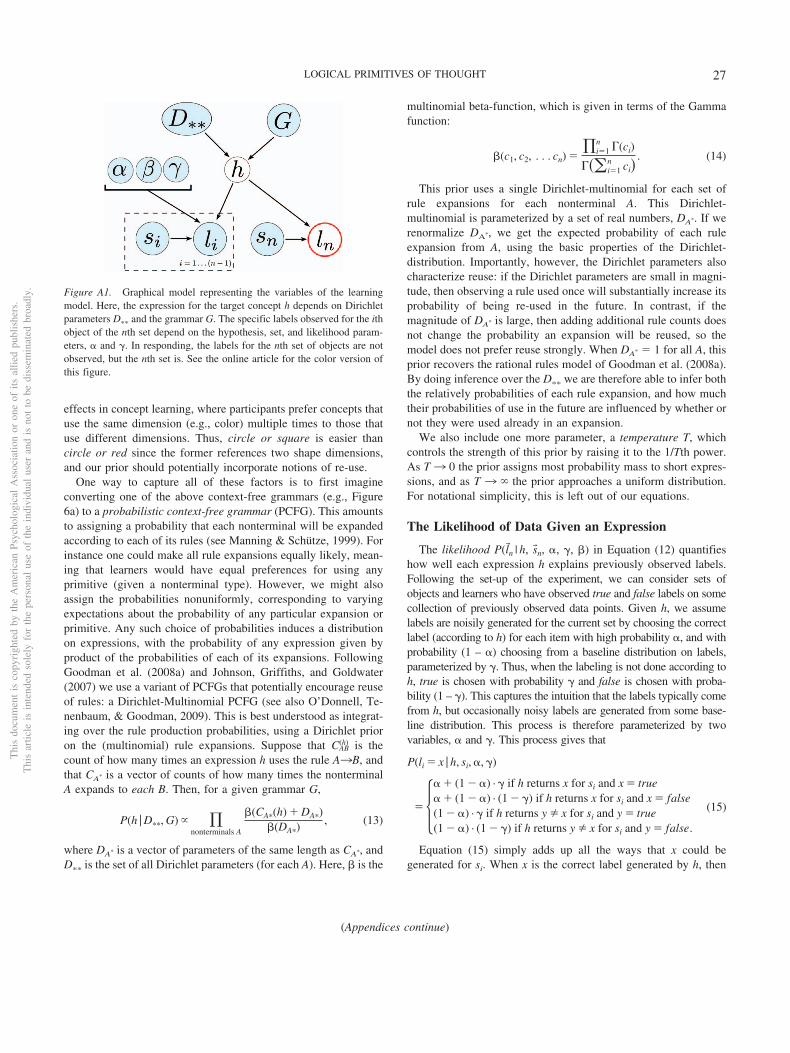
effects in concept learning, where participants prefer concepts thatuse the same dimension (e.g., color) multiple times to those thatuse different dimensions. Thus, circle or square is easier thancircle or red since the former references two shape dimensions,and our prior should potentially incorporate notions of re-use.

One way to capture all of these factors is to first imagineconverting one of the above context-free grammars (e.g., Figure6a) to a probabilistic context-free grammar (PCFG). This amountsto assigning a probability that each nonterminal will be expandedaccording to each of its rules (see Manning & Schütze, 1999). Forinstance one could make all rule expansions equally likely, mean-ing that learners would have equal preferences for using anyprimitive (given a nonterminal type). However, we might alsoassign the probabilities nonuniformly, corresponding to varyingexpectations about the probability of any particular expansion orprimitive. Any such choice of probabilities induces a distributionon expressions, with the probability of any expression given byproduct of the probabilities of each of its expansions. FollowingGoodman et al. (2008a) and Johnson, Griffiths, and Goldwater(2007) we use a variant of PCFGs that potentially encourage reuseof rules: a Dirichlet-Multinomial PCFG (see also O’Donnell, Te-nenbaum, & Goodman, 2009). This is best understood as integrat-ing over the rule production probabilities, using a Dirichlet prioron the (multinomial) rule expansions. Suppose that CAB

(h) is thecount of how many times an expression h uses the rule A¡B, andthat CA� is a vector of counts of how many times the nonterminalA expands to each B. Then, for a given grammar G,

P(h | D��, G) � �nonterminals A

�(CA�(h) DA�)�(DA�)

, (13)

where DA� is a vector of parameters of the same length as CA�, andD�� is the set of all Dirichlet parameters (for each A). Here, is the

multinomial beta-function, which is given in terms of the Gammafunction:

�(c1, c2, . . . cn) ��i�1

n�(ci)

��i�1n ci�

. (14)

This prior uses a single Dirichlet-multinomial for each set ofrule expansions for each nonterminal A. This Dirichlet-multinomial is parameterized by a set of real numbers, DA�. If werenormalize DA�, we get the expected probability of each ruleexpansion from A, using the basic properties of the Dirichlet-distribution. Importantly, however, the Dirichlet parameters alsocharacterize reuse: if the Dirichlet parameters are small in magni-tude, then observing a rule used once will substantially increase itsprobability of being re-used in the future. In contrast, if themagnitude of DA� is large, then adding additional rule counts doesnot change the probability an expansion will be reused, so themodel does not prefer reuse strongly. When DA� � 1 for all A, thisprior recovers the rational rules model of Goodman et al. (2008a).By doing inference over the D�� we are therefore able to infer boththe relatively probabilities of each rule expansion, and how muchtheir probabilities of use in the future are influenced by whether ornot they were used already in an expansion.

We also include one more parameter, a temperature T, whichcontrols the strength of this prior by raising it to the 1/Tth power.As T ¡ 0 the prior assigns most probability mass to short expres-sions, and as T ¡ � the prior approaches a uniform distribution.For notational simplicity, this is left out of our equations.

The Likelihood of Data Given an Expression

The likelihood P(�ln | h, s�n, �, �, ) in Equation (12) quantifieshow well each expression h explains previously observed labels.Following the set-up of the experiment, we can consider sets ofobjects and learners who have observed true and false labels on somecollection of previously observed data points. Given h, we assumelabels are noisily generated for the current set by choosing the correctlabel (according to h) for each item with high probability �, and withprobability (1 – �) choosing from a baseline distribution on labels,parameterized by �. Thus, when the labeling is not done according toh, true is chosen with probability � and false is chosen with proba-bility (1 – �). This captures the intuition that the labels typically comefrom h, but occasionally noisy labels are generated from some base-line distribution. This process is therefore parameterized by twovariables, � and �. This process gives that

P(li � x | h, si, �, �)

�� (1 �) · � if h returns x for si and x � true� (1 �) · (1 �) if h returns x for si and x � false(1 �) · � if h returns y � x for si and y � true(1 �) · (1 �) if h returns y � x for si and y � false.

(15)

Equation (15) simply adds up all the ways that x could begenerated for si. When x is the correct label generated by h, then


Figure A1. Graphical model representing the variables of the learningmodel. Here, the expression for the target concept h depends on Dirichletparameters D�� and the grammar G. The specific labels observed for the ithobject of the nth set depend on the hypothesis, set, and likelihood param-eters, � and �. In responding, the labels for the nth set of objects are notobserved, but the nth set is. See the online article for the color version ofthis figure.

Thi

sdo

cum

ent

isco

pyri

ghte

dby

the

Am

eric

anPs

ycho

logi

cal

Ass

ocia

tion

oron

eof

itsal

lied

publ

ishe

rs.

Thi

sar

ticle

isin

tend

edso

lely

for

the

pers

onal

use

ofth

ein

divi

dual

user

and

isno

tto

bedi

ssem

inat

edbr

oadl

y.


x could be generated by labeling from h with probability �, or bychoosing from the baseline distribution with probability (1 – �).This choice from the baseline depends on whether x is true(probability �) or x is false (probability 1 – �). If x is not the labelreturned by applying h to si, then it has to have been generatedfrom the baseline distribution. This equation embodies the assump-tion that learners reason about the statistical process that generatestheir observed data, allowing them to imagine how likely anyparticular hypothesis h would make the observed data, given thenoisy labeling process.

Equation (15) allows us to score the likelihood of the labelfor any particular labeled set of objects. But in the experiment,participants see a sequence of labeled sets and objects. It islikely that learners have better memory for more recent exam-ples, so we include a memory-decay on the likelihood, so that

learners prefer more strongly to get more recent examplescorrect. Motivated by power law decays in memory (Anderson& Schooler, 1991), this takes the form of a power law decay onthe log likelihood:

logP(�ln | h, s�n�, �, �) � �i�1

n

(n i 1)� logP(li | h, sn, �, �)

(16)

Here, we have weighted the likelihood of an individual set from(15) by a power-law term, (n – i � 1)�, which makes earlier dataless important. This introduces one free parameter, � 0, whichcontrols the amount of memory-decay in the model. For � 0,learners prefer hypotheses that explain more recent data, but as ¡ 0, this preference is reduced.

Appendix B

Inference for Data Analysis

Let rn(x) be the number of participants who labeled set sn with theset of labels x (one true/false response for each item in sn), and R theset of all human responses. In analyzing the data, we are interested inscoring the probability of any particular set of parameters given theparticipant responses. By Bayes rule, the probability

P(D��, �, �, � | G, R, s�n, �ln)

� P(R | G, D��, �, �, �, s�n, �ln)P(D��, �, �, �). (17)

The first term here is the likelihood of the human responses forany given setting of the parameters. Under the assumption thatparticipants choose labelings according to the output of the learn-ing model, this term is a multinomial likelihood,

P(R | G, D��, �, �, �, s�n, �ln)

� �i�1

n

�x

�P(li � x | s�i1, �li1, G, D��, �, �, �)ri(x) (18)

where product over x runs over all possible labelings x of si (allvalues of li). Equation (18) says that the probability of all re-sponses according to the learning model is a product over allsets observed, and for each set a product over all possiblelabelings raised to the number of times that labeling is observedin participants. The key term of (18) is the probability of anylabeling given all previous data, P(li � x | s�i1, �li1, G, D��, �,�, ), since this is the model’s predicted distribution of re-sponses to set i. This term is important because it characterizesthe model generalizations: the model works well if it generalizeslike people do, labeling new data from typically ambiguous evidencein the same way as our study participants. The target expression hdoes not appear here because the right h is not known to participants;

however, it can be computed using the previously defined prior (13)and likelihood (15):

P(li � x | s�i1, �li1, G, D��, �, �, �)

� �h�G

P(ln � x | h, si, �, �, �)P(h | s�n1, �ln1, G, D��, �, �, �).

(19)

Intuitively, participants’ distribution of guesses at ln is given bythe probability of ln given each hypothesis h, times the probabilitythat h is correct according to all previously labeled data.

The second term in Equation (17) is the prior on parameters. Wechoose these priors to have a very simple form: D�� is chosenaccording to a gamma (1, 2) prior and the priors on �, , and � aretaken to be uniform. In practice, the amount of data the model isfit to makes these priors largely irrelevant.

Together, these parts of Equation (17) specify a probabilisticdata analysis model that allows us to use the learning model toinfer a distribution on unknown parameters that characterize thegrammar and the likelihood. Until this point, we have presentedthis model as though there is only one concept and list; this was fornotational convenience since otherwise all variables would have tobe indexed by a concept (and potentially a list). The main param-eters of interest—D��, �, �, , and most importantly G—arepsychological variables that are true across concepts. Most of thepower of our analysis comes from finding parameters that work fora wide variety of concepts. So in reality, (18) involves a productover concepts.4

4 And so s�n and �ln must also be indexed by concept and list correspond-ingly.


Thi

sdo

cum

ent

isco

pyri

ghte

dby

the

Am

eric

anPs

ycho

logi

cal

Ass

ocia

tion

oron

eof

itsal

lied

publ

ishe

rs.

Thi

sar

ticle

isin

tend

edso

lely

for

the

pers

onal

use

ofth

ein

divi

dual

user

and

isno

tto

bedi

ssem

inat

edbr

oadl

y.


Appendix C

Formal Description of Alternative Models

Here we describe several additional models compared in theResults sections:

Uniform

This model assigns all hypotheses a uniform prior:

P(h) � 1. (20)

This prior is also improper and is an interesting baseline thatcorresponds to no substantive expectations about the form ofconcepts.

Response-Biased

This model corresponds to a simple response-biased modelwhich uses labeled data to do inference over the proportion of timethe hypothesis is true. This can be interpreted as a special repre-sentation language where there are only two possible expressions:one that is always true and one that is always false.

Logistic

This model provides another baseline which fits a logistic learn-ing curve within each concept. This model therefore has no inter-esting representational capacities or predictive abilities, but com-parison to it reveals the degree to which LOT models can surpasshow a statistician or psychophysicist might model performance inthis task.

Exemplar

This is an exemplar model on the set-based stimuli. It is difficultto know exactly how exemplar models might be applied to sets of

objects, since such models are generally stated in terms of simi-larity of object features, not similarities of collections of objects.Here, we begin by defining an object-wise distance metric:

d(x, y) � shape(x)�shape(y) · Wshape

color(x)�color(y) · Wcolor

size(x)�size(y) · Wsize,

where shape, color, and size are functions that map objects to theirshapes, colors, and sizes, and Wshape, Wcolor, and Wsize are freeparameters. Given two sets, we can then consider all possible waysof aligning their objects. This is necessary because if the next setis similar to a previously observed set, we need to know howobjects in the current set correspond to objects in the previous one.Since their orders may change, this can only be accomplished byfinding an alignment between the sets. For convenience, letd�(sj,sk) be the total distance according to d of the best alignmentof elements of sets sj and sk. If the sets are different sizes, thensome elements may be dropped. Then we define a distance metricon sets by

D (sj, sk) � abs ( |sj| |sk| ) · Wlength d*(sj, sk). (21)

Intuitively, this says that sets are penalized Wlength for differ-ences in cardinality, and then according to the distance of theirelements in the best alignment via d(x, y). D is used to define theprobability of generalizing labels from a previously labeled sj tothe next set, sn, according to the best alignment between the two.This log probability is proportional to

�nj1 · log D(sj, sn). (22)

Like the Bayesian models, this includes a power law memory-decay parameter, .


Thi

sdo

cum

ent

isco

pyri

ghte

dby

the

Am

eric

anPs

ycho

logi

cal

Ass

ocia

tion

oron

eof

itsal

lied

publ

ishe

rs.

Thi

sar

ticle

isin

tend

edso

lely

for

the

pers

onal

use

ofth

ein

divi

dual

user

and

isno

tto

bedi

ssem

inat

edbr

oadl

y.


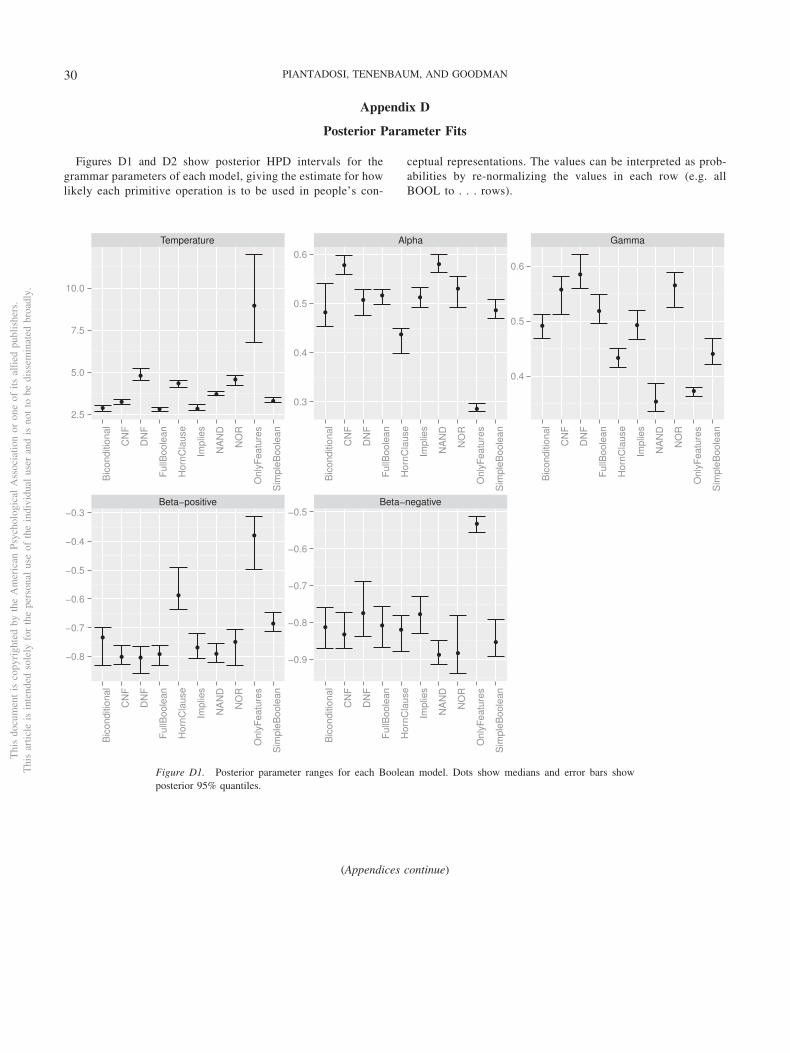
Appendix D

Posterior Parameter Fits

Figures D1 and D2 show posterior HPD intervals for thegrammar parameters of each model, giving the estimate for howlikely each primitive operation is to be used in people’s con-

ceptual representations. The values can be interpreted as prob-abilities by re-normalizing the values in each row (e.g. allBOOL to . . . rows).

Figure D1. Posterior parameter ranges for each Boolean model. Dots show medians and error bars showposterior 95% quantiles.


Thi

sdo

cum

ent

isco

pyri

ghte

dby

the

Am

eric

anPs

ycho

logi

cal

Ass

ocia

tion

oron

eof

itsal

lied

publ

ishe

rs.

Thi

sar

ticle

isin

tend

edso

lely

for

the

pers

onal

use

ofth

ein

divi

dual

user

and

isno

tto

bedi

ssem

inat

edbr

oadl

y.


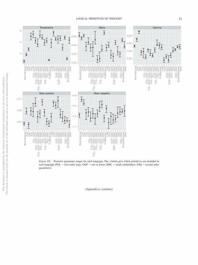
Figure D2. Posterior parameter ranges for each language. The x-labels give which primitives are included ineach language (FOL � first order logic; OOF � one or fewer; SMC � small cardinalities; 2OQ � second orderquantifiers).

(Appendices continue)Thi

sdo

cum

ent

isco

pyri

ghte

dby

the

Am

eric

anPs

ycho

logi

cal

Ass

ocia

tion

oron

eof

itsal

lied

publ

ishe

rs.

Thi

sar

ticle

isin

tend

edso

lely

for

the

pers

onal

use

ofth

ein

divi

dual

user

and

isno

tto

bedi

ssem

inat

edbr

oadl

y.


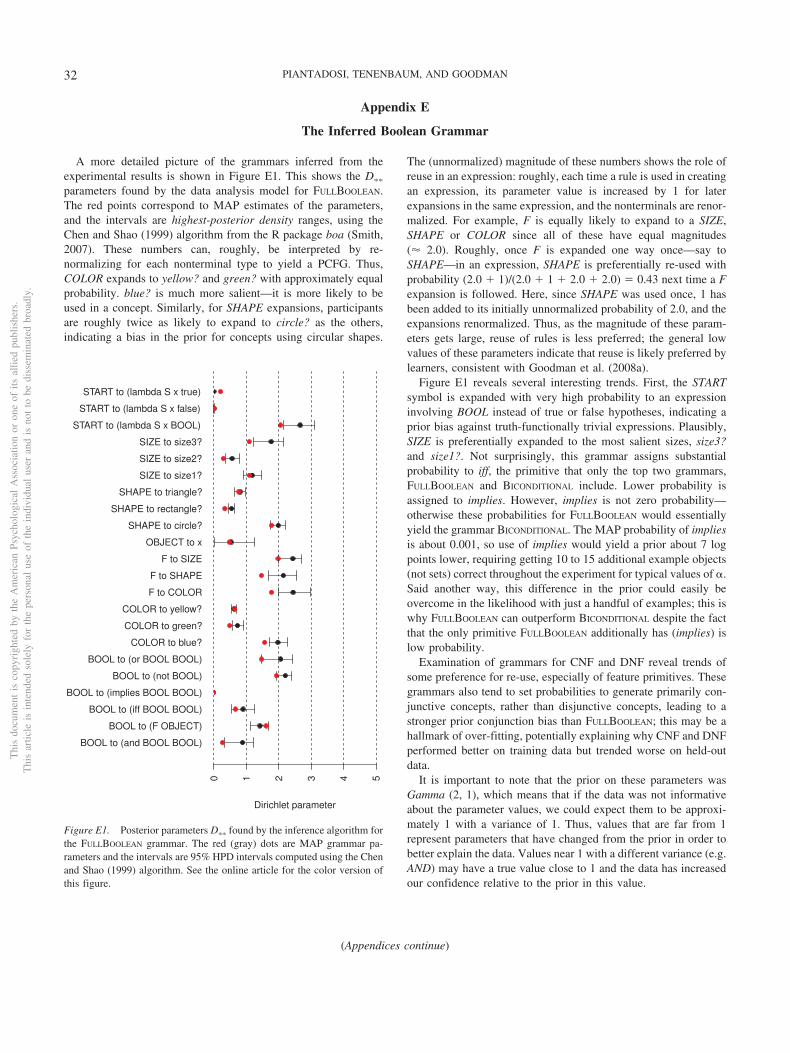
Appendix E

The Inferred Boolean Grammar

A more detailed picture of the grammars inferred from theexperimental results is shown in Figure E1. This shows the D��

parameters found by the data analysis model for FULLBOOLEAN.The red points correspond to MAP estimates of the parameters,and the intervals are highest-posterior density ranges, using theChen and Shao (1999) algorithm from the R package boa (Smith,2007). These numbers can, roughly, be interpreted by re-normalizing for each nonterminal type to yield a PCFG. Thus,COLOR expands to yellow? and green? with approximately equalprobability. blue? is much more salient—it is more likely to beused in a concept. Similarly, for SHAPE expansions, participantsare roughly twice as likely to expand to circle? as the others,indicating a bias in the prior for concepts using circular shapes.

The (unnormalized) magnitude of these numbers shows the role ofreuse in an expression: roughly, each time a rule is used in creatingan expression, its parameter value is increased by 1 for laterexpansions in the same expression, and the nonterminals are renor-malized. For example, F is equally likely to expand to a SIZE,SHAPE or COLOR since all of these have equal magnitudes(� 2.0). Roughly, once F is expanded one way once—say toSHAPE—in an expression, SHAPE is preferentially re-used withprobability (2.0 � 1)/(2.0 � 1 � 2.0 � 2.0) � 0.43 next time a Fexpansion is followed. Here, since SHAPE was used once, 1 hasbeen added to its initially unnormalized probability of 2.0, and theexpansions renormalized. Thus, as the magnitude of these param-eters gets large, reuse of rules is less preferred; the general lowvalues of these parameters indicate that reuse is likely preferred bylearners, consistent with Goodman et al. (2008a).

Figure E1 reveals several interesting trends. First, the STARTsymbol is expanded with very high probability to an expressioninvolving BOOL instead of true or false hypotheses, indicating aprior bias against truth-functionally trivial expressions. Plausibly,SIZE is preferentially expanded to the most salient sizes, size3?and size1?. Not surprisingly, this grammar assigns substantialprobability to iff, the primitive that only the top two grammars,FULLBOOLEAN and BICONDITIONAL include. Lower probability isassigned to implies. However, implies is not zero probability—otherwise these probabilities for FULLBOOLEAN would essentiallyyield the grammar BICONDITIONAL. The MAP probability of impliesis about 0.001, so use of implies would yield a prior about 7 logpoints lower, requiring getting 10 to 15 additional example objects(not sets) correct throughout the experiment for typical values of �.Said another way, this difference in the prior could easily beovercome in the likelihood with just a handful of examples; this iswhy FULLBOOLEAN can outperform BICONDITIONAL despite the factthat the only primitive FULLBOOLEAN additionally has (implies) islow probability.

Examination of grammars for CNF and DNF reveal trends ofsome preference for re-use, especially of feature primitives. Thesegrammars also tend to set probabilities to generate primarily con-junctive concepts, rather than disjunctive concepts, leading to astronger prior conjunction bias than FULLBOOLEAN; this may be ahallmark of over-fitting, potentially explaining why CNF and DNFperformed better on training data but trended worse on held-outdata.

It is important to note that the prior on these parameters wasGamma (2, 1), which means that if the data was not informativeabout the parameter values, we could expect them to be approxi-mately 1 with a variance of 1. Thus, values that are far from 1represent parameters that have changed from the prior in order tobetter explain the data. Values near 1 with a different variance (e.g.AND) may have a true value close to 1 and the data has increasedour confidence relative to the prior in this value.


Figure E1. Posterior parameters D�� found by the inference algorithm forthe FULLBOOLEAN grammar. The red (gray) dots are MAP grammar pa-rameters and the intervals are 95% HPD intervals computed using the Chenand Shao (1999) algorithm. See the online article for the color version ofthis figure.

Thi

sdo

cum

ent

isco

pyri

ghte

dby

the

Am

eric

anPs

ycho

logi

cal

Ass

ocia

tion

oron

eof

itsal

lied

publ

ishe

rs.

Thi

sar

ticle

isin

tend

edso

lely

for

the

pers

onal

use

ofth

ein

divi

dual

user

and

isno

tto

bedi

ssem

inat

edbr

oadl

y.


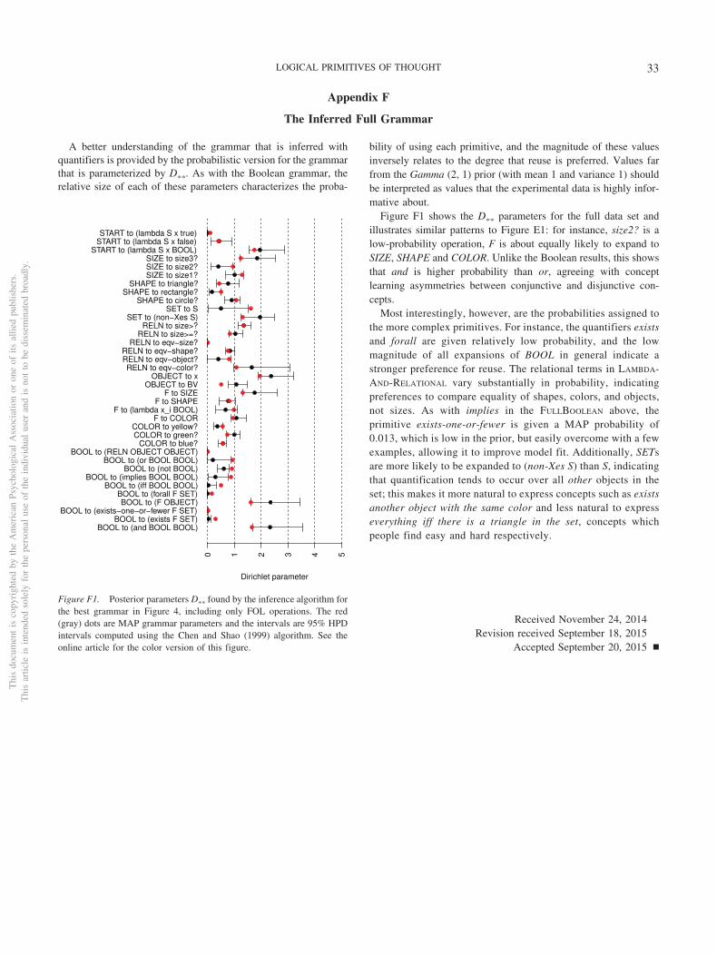
Appendix F

The Inferred Full Grammar

A better understanding of the grammar that is inferred withquantifiers is provided by the probabilistic version for the grammarthat is parameterized by D��. As with the Boolean grammar, therelative size of each of these parameters characterizes the proba-

bility of using each primitive, and the magnitude of these valuesinversely relates to the degree that reuse is preferred. Values farfrom the Gamma (2, 1) prior (with mean 1 and variance 1) shouldbe interpreted as values that the experimental data is highly infor-mative about.

Figure F1 shows the D�� parameters for the full data set andillustrates similar patterns to Figure E1: for instance, size2? is alow-probability operation, F is about equally likely to expand toSIZE, SHAPE and COLOR. Unlike the Boolean results, this showsthat and is higher probability than or, agreeing with conceptlearning asymmetries between conjunctive and disjunctive con-cepts.

Most interestingly, however, are the probabilities assigned tothe more complex primitives. For instance, the quantifiers existsand forall are given relatively low probability, and the lowmagnitude of all expansions of BOOL in general indicate astronger preference for reuse. The relational terms in LAMBDA-AND-RELATIONAL vary substantially in probability, indicatingpreferences to compare equality of shapes, colors, and objects,not sizes. As with implies in the FULLBOOLEAN above, theprimitive exists-one-or-fewer is given a MAP probability of0.013, which is low in the prior, but easily overcome with a fewexamples, allowing it to improve model fit. Additionally, SETsare more likely to be expanded to (non-Xes S) than S, indicatingthat quantification tends to occur over all other objects in theset; this makes it more natural to express concepts such as existsanother object with the same color and less natural to expresseverything iff there is a triangle in the set, concepts whichpeople find easy and hard respectively.

Received November 24, 2014Revision received September 18, 2015

Accepted September 20, 2015 �

Figure F1. Posterior parameters D�� found by the inference algorithm forthe best grammar in Figure 4, including only FOL operations. The red(gray) dots are MAP grammar parameters and the intervals are 95% HPDintervals computed using the Chen and Shao (1999) algorithm. See theonline article for the color version of this figure.

Thi

sdo

cum

ent

isco

pyri

ghte

dby

the

Am

eric

anPs

ycho

logi

cal

Ass

ocia

tion

oron

eof

itsal

lied

publ

ishe

rs.

Thi

sar

ticle

isin

tend

edso

lely

for

the

pers

onal

use

ofth

ein

divi

dual

user

and

isno

tto

bedi

ssem

inat

edbr

oadl

y.


colala: the computation and language lab at uc berkeley

Documents