colloquium: mechanical formalisms for tissue dynamics · colloquium: mechanical formalisms for...

DOI 10.1140/epje/i2015-15033-4

Colloquium

Eur. Phys. J. E (2015) 38: 33 THE EUROPEANPHYSICAL JOURNAL E

Colloquium: Mechanical formalisms for tissue dynamics

Sham Tlili1, Cyprien Gay1,6,a, Francois Graner1,6,b, Philippe Marcq2, Francois Molino3,4,6, and Pierre Saramito5,6

1 Laboratoire Matiere et Systemes Complexes, Universite Denis Diderot - Paris 7, CNRS UMR 7057, 10 rue Alice Domon etLeonie Duquet, F-75205 Paris Cedex 13, France

2 Laboratoire Physico-Chimie Curie, Institut Curie, Universite Marie et Pierre Curie - Paris 6, CNRS UMR 168, 26 rue d’Ulm,F-75248 Paris Cedex 05, France

3 Laboratoire Charles Coulomb, Univ. Montpellier II, CNRS UMR 5221, Place Eugene Bataillon, CC070, F-34095 MontpellierCedex 5, France

4 Institut de Genomique Fonctionnelle, Univ. Montpellier I, Univ. Montpellier II, 141 rue de la Cardonille, CNRS UMR 5203,INSERM UMR S 661, F-34094 Montpellier Cedex 05, France

5 Laboratoire Jean Kuntzmann, Universite Joseph Fourier - Grenoble I, CNRS UMR 5524, BP 53, F-38041 Grenoble Cedex,France

6 Academy of Bradylogists - Paris Cedex 13, France

Received 27 September 2013 and Received in final form 22 December 2014Published online: 13 May 2015 – c© EDP Sciences / Societa Italiana di Fisica / Springer-Verlag 2015

Abstract. The understanding of morphogenesis in living organisms has been renewed by tremendousprogress in experimental techniques that provide access to cell scale, quantitative information both onthe shapes of cells within tissues and on the genes being expressed. This information suggests that ourunderstanding of the respective contributions of gene expression and mechanics, and of their crucial entan-glement, will soon leap forward. Biomechanics increasingly benefits from models, which assist the designand interpretation of experiments, point out the main ingredients and assumptions, and ultimately leadto predictions. The newly accessible local information thus calls for a reflection on how to select suitableclasses of mechanical models. We review both mechanical ingredients suggested by the current knowledgeof tissue behaviour, and modelling methods that can help generate a rheological diagram or a constitutiveequation. We distinguish cell scale (“intra-cell”) and tissue scale (“inter-cell”) contributions. We recall themathematical framework developed for continuum materials and explain how to transform a constitutiveequation into a set of partial differential equations amenable to numerical resolution. We show that whenplastic behaviour is relevant, the dissipation function formalism appears appropriate to generate consti-tutive equations; its variational nature facilitates numerical implementation, and we discuss adaptationsneeded in the case of large deformations. The present article gathers theoretical methods that can readilyenhance the significance of the data to be extracted from recent or future high throughput biomechanicalexperiments.

1 Introduction

1.1 Motivations

While biologists use the word “model” for an organismstudied as an archetype, such as Drosophila or Arabidop-sis, physicists rather use this word for models based on ei-ther analytical equations or numerical simulations. Biome-chanical models have a century-old tradition and playseveral roles [1]. For instance, they assist experiments tointegrate and manipulate quantitative data, and extractmeasurements of relevant parameters (either directly, or

a e-mail: [email protected] e-mail: [email protected]

through fits of models to data). They also lead to predic-tions, help to propose and design new experiments, testthe effect of parameters, simulate several realisations ofa stochastic phenomenon, or simulate experiments whichcannot be implemented in practice. They enable to illus-trate an experiment, favor its interpretation and under-standing. They point out the main ingredients and as-sumptions, test the sensitivity of an experiment to a pa-rameter or to errors, and determine which assumptions aresufficient to describe an experimental result. Models canhelp to determine whether two facts which appear similarhave a superficial or deep analogy, and whether two factswhich are correlated are causally related or not.

Two themes have dominated the recent literature:modelling the mechanics of some specific adult tissues like

of 31 Eur. Phys. J. E (2015) 38: 33

bones or muscles, for which deformations and stresses areobviously part of the biological function [2,3]; and unravel-ing the role of forces in the generation of forms during em-bryonic development [4,5]. During the last decades, boththe physics and the biology sides of the latter questionhave been completely transformed, especially by progressin imaging.

On the physics side, new so-called “complex” materi-als with an internal structure, such as foams, emulsions orgels, have been thoroughly studied, especially in the lasttwenty years, with a strong emphasis on the difficult prob-lem of the feedback between the microscopic structure andthe mechanical response [6,7]. The development of newtools to image the changes in the microstructure arrange-ment under well-controlled global stresses or deformationshas provided a wealth of data. Modelling has played a cru-cial part via the determination of so-called “constitutiveequations”. A constitutive equation characterises the localproperties of a material within the framework of contin-uum mechanics. It relates dynamical quantities, such asthe stress carried by the material, with kinematical quan-tities, e.g. the deformation (also called “strain”) or thedeformation rate.

On the biology side, questions now arise regarding theinterplay of cell scale behaviour and tissue scale mechan-ical properties, among which the following two examples.

A first question is: how does a collective behaviour,which is not obviously apparent at the cell scale, emerge atthe tissue scale? Analyses of images and movies suggestedthat epithelia or whole embryos behave like viscous liquidson long time scales [8]. The physical origin and the valueof the (effective) viscosity should be traced back to thecell dynamics: it can in principle incorporate contributionsfrom ingredients such as cell divisions and apoptoses [9]or cell contour fluctuations [10,11], but also from orien-tational order, cell contractility, cell motility or cell rheo-logical properties. All these local and sometimes changingingredients become progressively accessible to experimen-tal measurements. Biomechanical models can investigatethe bottom-up relationship between local cell scale struc-ture and tissue scale mechanical behaviour, unraveling thesignature of the cellular structure in the continuum me-chanics descriptions [10,11].

A second question is: how can the mechanical state ofthe tissue have an influence on the cell division rate [12,13], or on the orientation of the cells undergoing divi-sion [14]? In addition, the mechanical state of the tissuecan generate cell polarity and hence an anisotropy of thelocal cell packing, which may affect the mutual influencebetween the local mechanics (forces and deformations)and the cell behaviour. Biomechanical models contributeto disentangle these complex feedback loops and addresssuch top-down relationships.

To address these questions, a natural strategy is first toreconstruct the mechanics from the structural description,then to investigate the feedback between well-identifiedmechanical variables and the expression of specific genes.In particular, this interplay between genes and mechanicsis expected to be the key to the spontaneous construction

of the adult form in a developing tissue without an or-ganising center. Such problem in its full complexity willprobably require a “systems biology” approach based onlarge scale mapping of expression for at least tens of genes,coupled to a correct mechanical modelling on an extendedrange of scales in time and space, which in turn supposesexperimental setups able to produce the relevant geneticand mechanical data.

1.2 State of the art

Recent developments in in vivo microscopy yield access tothe same richness of structural information for living tis-sues as has already been the case for complex fluids. Thebiology of cells and tissues is now investigated in detail interms of protein distribution and gene expression, espe-cially during development [15]. It is possible to image thefull geometry of a developing embryonic tissue at cellularresolution [16–20], while visualising the expression of vari-ous genes of interest [21–23]. Mechanical fields such as thedeformation, deformation rate or plastic deformation rateare increasingly accessible to direct measurement. Severalfields can be measured quantitatively at least up to anunknown prefactor. This is the case for: distributions ofproteins (involved in cytoskeleton, adhesion or force pro-duction), via quantitative fluorescence [24]; elastic forcesand stresses, either by laser ablation of cell junctions [25]and tissue pieces [26], or through image-based force infer-ence methods [27–30]; even viscous stress fields, indirectlyestimated [23]. Other methods include absolute measure-ments of forces based on micro-manipulation [31], in situincorporation of deformable force sensors [32] or fluores-cence resonance energy transfer (FRET) [33].

In vitro assemblies of cohesive cells are useful exper-imental materials. Within a reconstructed cell assembly,each individual cell retains its normal physiological be-haviour: it can grow, divide, die, migrate. In the absence ofany regulatory physiological context, cells display small ornegligible variation of gene expression. Reconstructed as-semblies thus allow to separate the mechanical behaviourof a tissue from its feedback to and from genetics. Further-more, in the absence of any coordinated variation of thegenetic identity of constituent cells, spatial homogeneitymay be achieved. Simple, well-controlled boundary condi-tions can be implemented by a careful choice of the geom-etry, either in two or three dimensions.

In two dimensions, confluent monolayers are usuallygrown on a substrate used both as a source of exter-nal friction and as a mechanical sensor to measure localforces [34–36]. 2D monolayers facilitate experiments, sim-ulations, theory and their mutual comparisons [37–41]. 2Dimages are easier to obtain and can be analysed in detail;data are more easily manipulated, both formally and com-putationally.

In three dimensions, multi-cellular spheroids in a well-controlled, in vitro setting [10,12,42,43] are a good mate-rial to mimic the mechanical properties of tumors, andof homogeneous parts of whole organs, either adult orduring development. They are also useful for rheological

Eur. Phys. J. E (2015) 38: 33 of 31

studies [44,45], especially since they are free from contactwith a solid substrate. Although the full reconstructionof the geometry of multi-cellular spheroids at cellular res-olution remains challenging, it has progressed in recentyears [46].

1.3 Outline of the paper

A tissue can be seen as a cellular material, active in thesense that it is out of equilibrium due to its reservoir ofchemical energy, which is converted into mechanical workat or below the scale of the material’s constituents, thecells. A consequence of this activity is that force dipoles,as well as motion, are generated autonomously.

Our global strategy is as follows. We construct rheolog-ical diagrams based on insights concerning the mechanicsof the biological tissue of interest. One of the main insightsis a distinction between intra-cell mechanisms: elastic-ity, internal relaxation, growth, contractility, and inter-cellmechanisms: cell-cell rearrangement, division and apopto-sis. The transcription of the rheological diagrams withinthe dissipation function formalism provides local rheolog-ical equations. We show how this local rheology should beinserted into the balance equations of continuum mechan-ics to generate a complete spatial model expressed as aset of partial differential equations. This procedure is con-ducted not only in the usually treated case of small elasticdeformations, but also in the relevant, less discussed, caseof large elastic deformations.

Our hope is to provide a functional and versatile tool-box for tissue modelling. We would like to guide the choiceof approaches and of models according to the tissue un-der consideration, the experimental set-up, or the scien-tific question raised. We propose a framework for a ten-sorial treatment of spatially heterogeneous tissues. It issuitable to incorporate the data arising from the analysisof experimental data, which are increasingly often live mi-croscopy movies. Although the simplest applications con-cern in vitro experiments, often performed with epithelialcells, the same approach applies to a wide spectrum of liv-ing tissues including animal tissues during development,wound healing, or tumorigenesis.

This article is organised as follows. Section 2 makesexplicit our assumptions and arguments, then details theuse of the dissipation function formalism. Section 3 re-views mechanical ingredients suitable for the theoreticaldescription of a wide range of living tissues, both in vitroand in vivo, illustrated with worked out examples chosenfor their simplicity. Section 4 groups these ingredients toform models of more realistic applications. Section 5 sum-marizes and opens perspectives.

Appendix A examines the link between the scale ofdiscrete cells and the scale of the continuous tissue. Ap-pendix B provides more details on how to write and useequations within the dissipation function formalism. Ap-pendix C provides further examples of coupling with non-mechanical fields. Appendix D examines the requirementsto treat tissue mechanics at large deformation.

2 Choices and methods

In this section, we explain our choices and our assump-tions. Section 2.1 compares discrete and continuum ap-proaches. Section 2.2 compares rheological diagrams, hy-drodynamics, and the dissipation function formalisms.Section 2.3 discusses specific requirements to model cel-lular materials. Section 2.4 suggests how to incorporatespace dependence in constitutive equations to write par-tial differential equations.

2.1 A continuum rather than a discrete description

Models that describe tissue mechanical properties may bebroadly split into two main categories: bottom-up “cell-based” simulations and continuum mechanics models.

Direct cellular simulations are built upon the (suppos-edly known) geometry and rheology of each individual celland membrane. They generate a global tissue behaviourthrough the computation of the large-scale dynamics ofassemblies of idealised cells [47–57]. Simulations enable todirectly test the collective effect of each cell scale ingredi-ent, and of their mutual feedbacks. Also, they work wellover a large range of cell numbers, up to tens of thou-sands, and down even to a small number of cells, wherethe length scale of a single cell and that of the cell assem-bly are comparable.

A continuum approach requires the existence of an in-termediate length scale, larger than a typical cell size,yet smaller than the tissue spatial extension, and beyondwhich the relevant fields vary smoothly. The continuumrheology is captured through a constitutive equation relat-ing the (tensorial) stresses and deformations [58–66]. Thisrheological model is incorporated into the usual frame-work of continuum mechanics using fundamental princi-ples such as material and momentum conservation. Notethat continuum models have also been applied to vegetaltissues, as in plant growth [58,67].

Both categories are complementary and have respec-tive advantages. For the purpose of the present paper, wefavor the continuum approach, which incorporates moreeasily precise details of cellular rheology. When it suc-ceeds, a continuum approach yields a synthetic grasp ofthe relevant mechanical variables on an intermediate scale(i.e. averaged over many individual cells), and helps deal-ing with large tissues. It often involves a smaller numberof independent parameters than a discrete approach, andthis helps comparing with experimental observations.

In order to test and calibrate a continuum model, itis generally necessary to extract continuum informationfrom other sources such as discrete simulations or experi-ments on tissues with cell scale resolution. Analysis toolshave been developed in recent years to process segmentedexperimental movies in order to extract tensorial quan-tities from cell contours, which might include the elasticdeformation and the plastic deformation rate [68]; for com-pleteness, these tools are recalled in appendix A.1.

The continuum models describing amorphous cellularmaterials can be tensorial and can incorporate viscoelasto-

of 31 Eur. Phys. J. E (2015) 38: 33

Fig. 1. An example of a rheological diagram: the Oldroyd vis-coelastic fluid model [73]. A Maxwell element (spring of stiff-ness G1 in series with a dashpot of viscosity η1) is in parallelwith a dashpot of viscosity η2.

plastic behaviour [58,64,69–71]. In addition to the viscousand elastic behaviour expected for a complex fluid thatcan store elastic deformation in its microstructure, oneincorporates the ingredient of plasticity. It captures irre-versible structural changes, more specifically here i) localrearrangements of the individual cells (see fig. 2) ii) celldivision or iii) plasticity within the cell. A viscoelastoplas-tic model assembling these ingredients could capture thedifferent “short-time” phenomena described in sect. 3 andat the same time display a viscous liquid-like behaviouron longer time scales.

In the following, we choose to concentrate on contin-uum models, drawing inspiration both from models of(non-living) amorphous cellular materials such as liquidfoams [72], and from models of living matter that incorpo-rate ingredients such as cell division [9] and orientationalorder [65,66].

2.2 Choice of the dissipation function formalism

In this section, we discuss three complementary generalformalisms used to construct constitutive equations, in-differently in two or three dimensions: rheological dia-grams (sect. 2.2.1), hydrodynamics in its general sense(sect. 2.2.2) and dissipation function (sect. 2.2.3). For sim-plicity we consider here stress and other mechanical ten-sors only with symmetrical components, while in generalthese three formalisms can include antisymmetric contri-butions when required.

2.2.1 Rheological diagram formalism

Figure 1 represents a classical example of rheological dia-gram: the Oldroyd viscoelastic fluid model [73]. It consistsin a dashpot with viscosity η2 and deformation ε carry-ing the stress σ2 in parallel with a Maxwell element car-rying the stress σ1. This Maxwell element is itself madeof a spring (stiffness G1, deformation ε1) in series witha dashpot (viscosity η1, deformation ε2). The elementary

rheological equations read

ε = ε1 + ε2,

σ = σ1 + σ2,

σ2 = η2 ε,

σ1 = G1 ε1,

σ1 = η1 ε2. (1)

Eliminating ε1, ε1, ε2 and ε2 between eqs. (1) yields

σ +G1

η1σ =

η1 + η2

η1G1 ε + η2 ε. (2)

Equation (2) is a constitutive equation for the ensemble.Such a straightforward method is useful when physicalknowledge or intuition of the material and its mechanicalproperties is sufficient to determine the topology (nodesand links) of the diagram.

Note that the relationship between a rheological dia-gram and a constitutive equation is not one-to-one. Forinstance, a Maxwell element (linear viscoelastic liquid) inparallel with a dashpot is a diagram distinct from a Voigtelement (linear viscoelastic solid) in series with a dashpot,but both are associated to the same constitutive equation.Section 3.3 presents another example.

2.2.2 Hydrodynamic formalism

When non-mechanical variables are present, the rheologi-cal diagram formalism (sect. 2.2.1) is not sufficient to es-tablish the constitutive equation. Another formalism isnecessary to include couplings between mechanical andnon-mechanical variables.

A possible formalism is linear out-of-equilibrium ther-modynamics, also called “hydrodynamics” [74] althoughits range of application is much larger than the mechanicsof simple fluids. This approach has been highly successful,leading for instance to the derivation of the hydrodynam-ics of nematic liquid crystals (with the nematic directorfield as an additional, non-conserved hydrodynamic vari-able) [75,76]; the collective movements of self-propelledparticles [77,78] (which have been suggested to be anal-ogous with tissues dynamics [56]); or, more recently, ofsoft active matter (where a chemical field typically cou-ples to an orientational order parameter to be modeledseparately, e.g. cytoskeletal mechanics) [79,80].

Broadly speaking, hydrodynamics may be defined asthe description of condensed states of matter on slow timescales and at large length scales. Macroscopic behaviouris characterized by the dynamics of a small number ofslow fields (so-called “hydrodynamic fields”), related toconservation laws and broken continuous symmetries [74].On time scales long compared to the fast relaxation timesof microscopic variables, the assumption of local thermo-dynamic equilibrium leads to the definition of a thermo-dynamic potential as a function of all relevant (long-lived)thermodynamic variables and their conjugate quantities.Standard manipulations lead to the expression of the en-tropy creation rate as a bilinear functional of generalized

Eur. Phys. J. E (2015) 38: 33 of 31

Fig. 2. Cell rearrangement, also known as: intercalation,neighbour exchange, or T1 process [21,72]. Cells 2 and 3 areinitially in contact (left). Cells deform (center) and can reacha configuration with a new topology where cells 1 and 4 arenow in contact, then relax (right).

fluxes and forces. In the vicinity of thermodynamical equi-librium, generalized fluxes are expressed as linear combi-nations of generalized forces. Due to microreversibility, theOnsager symmetry theorem implies that cross-coefficientsmust be set equal (respectively, opposite) when fluxes andforces have equal (respectively, opposite) sign under timereversal [81,82].

The hydrodynamic formalism is physically intuitive.It is flexible and can accommodate a broad spectrum ofphysical quantities, as long as deviations from equilibriumcan be linearised. This approach is quite general since itrelies on thermodynamic principles and on the invarianceproperties of the problem under consideration. Constitu-tive equations may thus be written within the domain oflinear response as linear relationships between generalizedfluxes and forces.

2.2.3 Dissipation function formalism

However, not all materials are described by a linear force-flux relationship. In tissues, plastic events such as cell re-arrangements (fig. 2) have thresholds which break downthe linearity, and hydrodynamics (sect. 2.2.2) becomes in-adequate. Deriving constitutive equations requires a moregeneral formalism.

In the dissipation function formalism, the state of thematerial is described by the total deformation ε and bym ≥ 0 additional, independent, internal variables εk, with1 ≤ k ≤ m. These variables may be scalar, vectorial ortensorial. So-called “generalized standard materials” aredefined by the existence of the energy function E and thedissipation function D, which are continuous (not neces-sarily differentiable) and convex functions of their respec-tive arguments [83–85]:

E = E (ε, ε1, . . . , εm) , (3)D = D (ε, ε1, . . . , εm) . (4)

Here ε denotes the total deformation rate, and εk is the(Lagrangian) time derivative of εk. Although it is rarelyexplicitly stated, these energy and dissipation functionsshould increase when the norms of their arguments tendto infinity, so that they admit one (and only one) mini-mum, reached for a finite value of their arguments. Consti-tutive and evolution equations are obtained through the

following rules, where σ denotes the stress:

σ =∂D∂ε

+∂E∂ε

, (5)

0 =∂D∂εk

+∂E∂εk

, 1 ≤ k ≤ m. (6)

Appendix B provides more details on how to use the dis-sipation function formalism. In particular, appendix B.1explains how to manipulate the corresponding equations.Appendix B.2 explicitly treats the tensorial case, andshows that the tensorial variables in eqs. (3), (4) shouldbe decomposed into their trace and deviatoric parts:

E = E (tr ε, tr ε1, . . . ,dev ε,dev ε1, . . .) , (7)D = D (tr ε, tr ε1, . . . ,dev ε,dev ε1, . . .) , (8)

considered as independent variables. Appendix B.3 explic-its the incompressible case.

The formalism of eqs. (3)-(6) is a convenient tool forbuilding complex models and obtaining in a systematicway the full set of partial differential equations from sim-ple and comprehensive graphical schemes. The couplingcoefficients arise as cross partial derivatives, with the ad-vantage that they derive from a smaller number of freeparameters than in the hydrodynamics formalism.

For purely mechanical diagrams made of springs, dash-pots and sliders, the dissipation function formalism yieldsthe same equations as when directly writing the dynam-ical equations from the rheological model, as shown inappendix B.4. The same formalism also applies to sys-tems with non-mechanical variables, see sect. 3.4 and ap-pendix C.

A direct link between the hydrodynamic and dissipa-tion function formalisms can be established when the dis-sipation function D is a quadratic function of its argu-ments. For a given variable εk, quadratic terms ε2

k in theenergy function or ε2

k in the dissipation function are har-monic, i.e. they yield a linear term εk or εk in the deriveddynamical equations, exactly like in the hydrodynamicsformalism (sect. 2.2.2). In this case, D is proportional tothe rate of entropy production [82] (this is also true forviscoplastic flows [86]).

The dissipation function formalism is also suitable fornonlinear terms. Terms of the form |εk|n or |εk|n, withn ≥ 1 (n integer or real) yield nonlinear terms |εk|n−2εk

or |εk|n−2εk in the dynamical equations.Interestingly, the dissipation function can even include

the particular case n = 1 which corresponds to terms like|εk| or |εk|. This yields terms of the form εk/|εk| or εk/|εk|in the derived equations: these are nonlinear terms whichdominate over the linear ones. This lowest-order case isuseful to include plasticity (see sect. 3.1 for an example),whose treatment thus becomes straightforward [84–86]:the dissipation function formalism has been successfullyapplied to viscoelastoplastic flows [87,88]. As discussedin sect. 3.1, regularizing such terms would suppress yieldstress effects.

Since the cross coupling coefficients arise as cross par-tial derivatives, they are by construction always equal by

of 31 Eur. Phys. J. E (2015) 38: 33

pairs. The Onsager symmetry theorem [81] is thus imme-diately obeyed when fluxes and forces behave similarly un-der time reversal, but not if they behave differently. Notethat this is compatible with the constitutive equations ofliving tissues: since microreversibility may not apply at the(cell) microscale, the Onsager symmetry theorem does notneed to apply.

Active ingredients which impose a force, a deforma-tion rate, or a combination thereof, can be included in thedissipation function formalism, as shown for instance insect. 3.3. The functions E and D remain convex and stillreach a minimum for a finite value of their arguments.As expected, the entropy creation rate is no longer al-ways positive.

From a mathematical point of view, the large set ofnonlinear differential equations is known to be well posedin the Eulerian and small deformation setting [89]. Sincethe free energy function E and the dissipation functionD are both convex, in the case of small deformations theexistence and uniqueness of solution is guaranteed, whilethe second law of thermodynamics is automatically satis-fied [83,85]. This is a major advantage of the dissipationfunction framework.

In addition, the formalism is also effective from acomputational point of view. For problems which involvemulti-dimensional and complex geometries together withlarge deformations of the tissue, there is no hope to ob-tain an explicit expression of the solution: its computa-tion should be obtained by an approximation procedure.The resolution of the large set of nonlinear differentialequations and its convergence at high accuracy requireboth a dedicated algorithm and a large computing timewith the present computers. The convexity of E and Dfunctions enables to use robust optimization algorithmsto solve efficiently the set of dynamical equations thanksto variational formulations [90,91]. This second major ad-vantage of the dissipation function framework has beenwidely used in small deformation, for applications in solidmechanics and plasticity, and has allowed the developmentof robust rocks and soils finite element modeling softwares(see e.g. [86,89] and references therein).

In summary, since the dissipation function formalismallows to treat plasticity and is convenient for numericalresolution, we recommend to adopt it for living tissues.

2.3 Specificity of cellular material modelling

While continuum mechanics is standard, cellular materialmodelling requires care on specific points. They include:the separation of the deformation between its contribu-tion arising from inside each cell and from the mutual cellarrangement (sect. 2.3.1); the choice of Eulerian ratherthan Lagrangian description for a viscous, elastic, plasticmaterial (sect. 2.3.2); and the treatment of large elasticdeformations (sect. 2.3.3).

2.3.1 Intra-cell and inter-cell deformation

Different deformation rates can be measured simultane-ously and independently (see appendices A.1 and D.1).

Fig. 3. Decomposition of the tissue deformation rate ε intothe deformation rate εintra of the constituent cells and the de-formation rate εinter that reflects inter-cell relative velocities(eq. (9)).

The total deformation rate ε can be measured by track-ing the movements of markers, moving with the tissue asif they were pins attached to the tissue matter. This totaldeformation rate originates from the following two contri-butions at the cellular level.

The intra-cellular deformation rate εintra is the averageof the deformation rate as perceived by individual cells,where each cell is only aware of the relative positions ofits neighbours. The intra-cellular deformation εintra canbe measured by observing the anisotropy of a group oftracers attached to a reference cell and its neighbours, fol-lowed by an average over reference cells. By contrast withε, the tracers are not attached permanently to the tissueitself: when neighbours rearrange and lose contact withthe reference cell, the corresponding tracers are switchedimmediately to the new neighbours. The intra-cell defor-mation rate εintra is then obtained as the rate of changeof this intra-cell deformation measure εintra.

The inter-cellular deformation rate εinter reflects thecell rearrangements and relative movements. It can bemeasured by tracking the rearrangements themselves.

In tissues made of cells which tile the space, the stressat the tissue scale is the stress carried by the cells them-selves (like in foams, but as opposed e.g. to the case ofplants, where the rigid walls are as important as pressurefor stress transmission). We thus advocate a decomposi-tion in series, where intra- and inter-cellular stresses areequal, while intra- and inter-cellular deformation rates addup (fig. 3):

ε = εintra + εinter. (9)

Choosing this decomposition into intra-cell and inter-cellcontributions in series has consequences on the argumentsof the dissipation function. When defining the εk variables,see eqs. (3), (4), it is relevant to choose one of them asequal to εintra. Appendix D.1.2 discusses the case of largedeformations.

2.3.2 An Eulerian rather than a Lagrangian approach

We now compare the Lagrangian and Eulerian points ofview, and explain why we choose the latter.

For materials that retain information about their ini-tial state, it is natural (and common) to use a deformation

Eur. Phys. J. E (2015) 38: 33 of 31

variable, often denoted ε, that compares the current localmaterial state to the initial state of the same materialregion. This is called the Lagrangian description and isusually preferred for elastic solids [92]. The deformationrate ε of the Lagrangian description is the time derivativeof the deformation ε, where the dot denotes the materialderivative used for small deformations, ∂t + v · ∇:

ε =∂ε

∂t+ v · ∇ε. (10)

On the other hand, when plastic or viscous flows erasemost or all memory of past configurations, it is commonpractice to use only the current velocity field v(x, t) as themain variable, with no reference to any initial state. Thisis called the Eulerian description, used for instance whenwriting the Navier-Stokes equations.

Both descriptions are tightly connected: the defor-mation rate ε of the Lagrangian description is equal tothe (symmetric part of the) gradient of the velocity fieldv(x, t) of the Eulerian description:

ε =∇v + ∇vT

2. (11)

See eqs. (D.6), (D.8) for the complete expression at largedeformations.

The separation of intra- and inter-cellular dynamics,discussed in sect. 2.3.1, can be viewed as mixing the La-grangian and Eulerian points of view. Since cells retaintheir integrity, the quantity εintra is similar to a defor-mation variable in a Lagrangian approach. By contrast,the relative motions of cells (described by εinter) is similarto the relative motions of material points in usual fluids,described from an Eulerian point of view.

A globally Eulerian description has been implementedfor liquid foams in a direct manner, based on the argumentthat the rearrangement deformation rate εinter progres-sively erases from the material the memory of the initialconfiguration and thus progressively wipes, like in com-mon fluids, the relevance of the material deformation εfor predicting the future evolution of the material [69].

Here, the same argument should apply. In the exam-ples provided in sect. 3 the variables εinter and ε naturallydisappear from the final constitutive equation, and onlytheir corresponding deformation rates εinter and ε con-tribute. This reflects the absence of any structure holdingcells together beyond the first neighbours. It confirms therelevance of an Eulerian description for a material such asa tissue.

2.3.3 Large elastic deformations

For pedagogical reasons, in the present article, all equa-tions are written within the limit of small elastic deforma-tions. Yet, in living tissues, large elastic deformations areencountered.

Appendix D explains in details how to model large de-formations in the specific context of tissue mechanics, and

reformulate accordingly the dissipation function formal-ism. In particular, it discusses the volume evolution, theelasticity and its transport, and the intra-cell deformation.

An example of changes due to large deformations is thedistinction between two quantities which are equal in thelimit of small deformations (eq. (11)): the deformation rateand the symmetrised velocity gradient (eqs. (D.6), (D.8)).The transport of large elastic deformations involves ob-jective derivatives. Several such derivatives exist, for in-stance lower- and upper-convected derivatives, as well asGordon-Schowalter derivatives which interpolate betweenthem. In rheological studies of complex fluids, the selec-tion of the derivative is often motivated by formal reasons,or is empirical. In appendix D.1.1, for physical reasons, wedescribe the deformation using tensors attached to the cel-lular structure; we show that this choice selects univocallythe upper-convected derivative.

2.4 Set of partial differential equations

A tissue may be spatially heterogeneous: its material prop-erties, its history, its interaction with its environment areunder genetic control and may depend on the position x.For instance the tissue may comprise different cell types,or it may be placed on a spatially modulated substrate.

The parameters and variables which describe the tis-sue are fields that may vary spatially. Here, we consideronly tissues amenable to a continuum mechanics descrip-tion, namely tissues whose relevant fields are smooth andslowly variable over the scale of a group of cell (the “rep-resentative volume element” of the continuum mechanicsdescription). In what follows, we assume that the fieldsare continuous and differentiable.

The evolution of the tissue is then expressed as a setof partial differential equations (PDE), consisting in con-servations laws and constitutive equations. To make thisarticle self-contained, we show in the present Section howconstitutive relations, such as derived using the dissipa-tion function formalism, can be embedded in the rigorousframework of continuum mechanics in order to obtain aclosed set of evolution equations.

In continuum mechanics, one usually starts from theconservation equations of mass, momentum and angularmomentum. The mass conservation equation reads

∂ρ

∂t+ ∇ · (ρv) = s, (12)

where ρ is the mass density (or mass per unit area in 2D);and s represents material sources or sinks which, in thecontext of a tissue, can be linked with cell growth andapoptosis, respectively, see sect. 3.2.2.

In general, the conservation of momentum reads:

ρa(x, t) = ∇ · σ(x, t) + f(x, t) (13)

which relates the acceleration a = ∂v∂t + (v · ∇)v to the

internal stress tensor σ and the external forces f . For in-stance, the external force f may contain a friction compo-nent f = −ζv [26,38,41]. Note that, in a tissue, the iner-tial term ρa is generally negligible when compared to the

of 31 Eur. Phys. J. E (2015) 38: 33

stress term ∇ · σ. The validity of this approximation hasto be checked in specific examples by estimating the valueof the relevant dimensionless number, e.g. the Reynoldsnumber for a purely viscous material, or the elastic num-ber for a purely elastic solid. In this case, the conservationof momentum (eq. (13)) reads

∇ · σ(x, t) + f(x, t) = 0. (14)

Finally, the conservation of angular momentum impliesthat the stress tensor is symmetric [74]: σij = σji.

We obtain a set of m + 4 evolution equations(eqs. (5), (6), (11), (12), (14)). There are m + 4 unknownfields: σ, (εk)1≤k≤m, ε, ρ and v. For any value d of thespace dimension, the number of coordinates of the un-known fields always equals the number of equations. Thisset of partial differential equations is closed by suitableinitial conditions on the same variables and d boundaryconditions in terms of velocity, deformation and/or stresscomponents. Its solution can be estimated by numericalresolution: see e.g. [70,90,91,93,94] for such numericalmethods in the context of liquid foam flows.

3 Ingredients included in tissue modelling

A (non-exhaustive) list of ingredients for tissue modellingincludes viscosity, elasticity, plasticity, growth, contractil-ity, chemical concentration fields, cell polarity, and theirfeedbacks. Note that other tissue-specific ingredients suchas (possibly active) boundary conditions [41] do not con-tribute to constitutive equations themselves: they are usedto solve the set of partial differential equations (estab-lished in sect. 2.4).

In sects. 3.1 to 3.4, we present four worked out exam-ples showing how such ingredients are taken into accountwithin the dissipation function formalism. Each choice inthis section is motivated by the simplicity (rather than bythe formalism, as in sect. 2, or by the realism, as in sect. 4).Section 3.5 combines individual ingredients into a compos-ite rheological model by classifying them in terms of shapeor volume contributions at the intra-cell or inter-cell level,and derives the corresponding set of equations.

3.1 Plasticity

3.1.1 Rearrangements and plastic deformation rate

Recent experiments performed on cell aggregates and cellmonolayers have shown that these tissues can have ayield stress [39,45] and display a plastic behavior [10,95].The origin of this plasticity includes cell rearrangements(fig. 2) [96,97] which also play an important role duringdevelopment, as in e.g. convergence-extension [15].

At the cell scale, and independently of its biological ori-gin and regulation, a cell rearrangement is mathematicallyspeaking a discontinuous topological process in a group ofneighbouring cells. The associated mechanical description

is decomposed into several steps. Before the rearrange-ment, the cells deform viscoelastically. During the rear-rangement, two cells in contact get separated. Both othercells establish a new contact. They all eventually relax to-wards a new configuration with the consequence that twocells have got closer while the others have moved apart.

Upon coarse-graining spatially at a scale of severalcells, and temporally over a time scale much larger thanthe relaxation time, the discontinuities at the cell scale arewiped out. The net result is an irreversible change in thestress-free configuration of the tissue, with convergencealong one axis and extension along the perpendicular one.It is thus best described as a tensor with positive and neg-ative eigenvalues [68,69], which tends towards the plasticdeformation rate εp in the continuum limit. This tensor isthe difference between the total deformation rate ε and theelastic deformation rate εe, so that the cumulated effectof elastic and plastic contributions add up:

ε = εe + εp. (15)

3.1.2 Plasticity and dissipation function

In the dissipation function formalism, elastoplastic andviscoelastoplastic materials are classically described byadding in the dissipation energy a yield stress term, forinstance proportional to the norm of the deformation rate(sect. 2.2.3). Such non-analytic term is fully compatiblewith the formalism. The convexity of the energy functionis preserved, so that equations are readily written and canbe solved using known numerical approaches. For details,see ref. [98].

When writing equations, physicists often favor smooth(analytic) expressions rather than discontinuous (singu-lar) ones. Formally, it would of course be possible to reg-ularize the plasticity equations and obtain a differentiabledissipation function by replacing each non-analytical termwith analytic, strong non-linearities. However, this wouldlead to a completely different category of models, fromwhich yield stress effects are absent and the solid be-haviour vanishes in the long time limit.

3.1.3 A viscoelastoplastic example

We treat explicitly an example obtained by adding an elas-tic element of modulus G in series with a diagram repre-senting a Bingham fluid, namely the combination in par-allel of a dashpot of viscosity η and a slider of yield stressσY (fig. 4). A more realistic (and therefore more complex)rheological model of a tissue that includes plasticity istreated in sect. 4.1.

According to fig. 4, we have

ε = ε1 + ε2. (16)

Choosing ε and ε2 as independent variables, the energyfunction reads

E(ε, ε2) =12Gε2

1 =12G (ε − ε2)

2 (17)

Eur. Phys. J. E (2015) 38: 33 of 31

Fig. 4. Rheological diagram for a plastic material. An elasticelement of modulus G is in series with a viscoplastic (Bingham)fluid, namely a dashpot of viscosity η in parallel with a sliderof yield stress σY.

and the dissipation function

D(ε, ε2) =12ηε2

2 + σY|ε2|. (18)

From eqs. (5), (6) we obtain

σ =∂D∂ε

+∂E∂ε

= G(ε − ε2), (19)

0 =∂D∂ε2

+∂E∂ε2

= ηε2 + σYε2

|ε2|− G(ε − ε2), (20)

which together yields the constitutive equation

σ = σYε2

|ε2|+ ηε2. (21)

When ε2 = 0, σ takes a value in the interval [−σY; +σY]:for a rigorous mathematical analysis, see ref. [88], and inparticular its eqs. (9), (10).

3.2 Growth

3.2.1 Conservation equations

The growth of a tissue has two aspects: mass growth andcell concentration growth. The mass growth affects themass conservation (eq. (12)) through its source term s =αg ρ, where αg is the rate of variation of mass density,which has the dimension of an inverse time

∂tρ + div(ρv) = αg ρ. (22)

Similarly, the cell concentration c (number of cells per unitvolume) evolves according to

∂tc + div(cv) = αc c, (23)

where αc is the rate of variation of the cell concentration.If we consider a tissue without gaps between cells, it is

reasonable to write that the mass density ρ is a constant,which simplifies the description. Equation (22) reduces to

div(v) = αg. (24)

Fig. 5. Cell growth modes in a tissue. Cells may swell (ratersw); undergo cytokinesis (rate rck); or both successively, re-sulting in a cell cycle (rate rcc). They may die by apoptosis(rate rapo) or necrosis (rate rnec).

Equation (A.7) indicates how to locally measure αg. Fora monolayer of varying thickness h but homogeneous andconstant density ρ, eq. (22) can be rewritten using thetwo-dimensional divergence applied in the plane of themonolayer, div2d

∂th + div2d(hv) = αgh. (25)

3.2.2 Cell growth modes

Several cell processes alter the tissue volume, the cell con-centration, or both (fig. 5). They are compatible with thedissipation function formalism, see for instance sect. 4.2.1.All rates are noted r and have the dimension of the inverseof a time (for instance typically a few hours or a day forthe division rate of epithelial cells in vitro [99]). For eachprocess, the corresponding r is the proportion of cells thatundergo the process per unit time. Each process becomesrelevant as soon as the duration of an experiment is of theorder of, or larger than, the inverse of its rate r.

Cells may grow, i.e. swell, with rate rsw, which createsvolume and decreases c. They may undergo cytokinesis,i.e. split into daughter cells, which increases c with rate rck

(c doubles in a time ln 2/rck) without altering the volume.In the case where the swelling and cytokinesis rates areequal, and their common value is the cell-cycle rate rcc =rsw = rck, the long-time average of cell size is constant. Forsimplicity, the description of cytokinesis proposed in thissection is scalar. More generally, one may need to definea tensor εck, with rck = tr εck (see sect. 3.5.1).

Cells may undergo necrosis (rate rnec), which doesnot alter the tissue volume but decreases the concentra-tion c of living cells. The description of apoptosis (raterapo), namely cell death under genetic control, requiressome care. If the content of the apoptosed cell materialis eliminated (for instance diffuses away, or is cleaned bymacrophages) without being taken up by the neighbour-ing cells; and if we further assume that the tissue remainsconnective (i.e., neighbouring cells move to span the emp-tied region); then apoptosis causes the tissue volume todecrease while c remains unaltered.

of 31 Eur. Phys. J. E (2015) 38: 33

Fig. 6. Model for growth in the presence of elasticity. Theactive deformation rate, here the growth rate αg, is constant,and the spring has a stiffness G.

The mass and cell concentration growth rates (definedin sect. 3.2.1) are

αg = rsw − rapo, (26)αc = rck − rsw − rnec. (27)

A first special case is the situation where cells undergocytokinesis without growing, hence leading to a decreaseof the average cell size, as encountered for example duringthe first rounds of cytokineses in a developing embryo.In that case, only the cell concentration has a non-zerosource, and eqs. (26), (27) reduce to

αg = 0, (28)αc = rck. (29)

In the situation that combines cell swelling and cytokinesisat equal rates, in equal amounts, and in the presence ofapoptosis, eqs. (26), (27) reduce to

αg = rcc − rapo, (30)αc = 0. (31)

3.2.3 A one-dimensional example

We illustrate with a one-dimensional example the casewhere cell swelling and cytokinesis rates are equal, re-sulting in a constant long-time average cell size. Here, weassume that after a full cell cycle the rest length of eachdaughter cell, defined as the length where their elastic en-ergy is lowest, is eventually identical to that of the mothercell. Appendix A.3 describes a tissue made of elastic cellswhich divide and/or die; it shows that the stress evolutionequation reads

σ � G (ε − αg). (32)

Equation (32) expresses that as expected, the stress(counted positive when tensile), increases when the tissueis subjected to elongation and decreases when the growthrate increases the tissue rest length [100,101].

Equation (32) can be derived from the rheological dia-gram shown in fig. 6, as follows. Consider a motor workingat constant deformation rate, here the growth rate αg, inseries with a spring of stiffness G. It creates a differencebetween the total deformation rate ε and the deformationrate εe of the spring

εe = ε − αg. (33)

Fig. 7. Two equivalent models of contractility. (a) With a con-stant active stress σact. (b) With a constant active deformationrate εact.

Combined with the elasticity

σ = Gεe (34)

this yields (32).When used in the dissipation function formalism,

eq. (33) which relates εe, ε and αg, is a topological re-lation and can be used in the same way as eq. (16).

3.3 Contractility

In tissues, cell scale contractility is often determined bythe distribution of molecular motors such as myosin II.Upon coarse-graining, this distribution translates into tis-sue scale contractility. In one dimension, such contractilitymay be modelled by a constant stress, as done in classi-cal models of muscle mechanics [102]. As an example, westudy the rheological diagram of fig. 7a, where within aMaxwell model (spring and dashpot in series) a contractileelement is placed in parallel with the dashpot.

Choosing ε and for instance ε2 as independent vari-ables (with ε = ε1 + ε2), the energy and dissipation func-tions can be written in the form of eqs. (3), (4), withm = 1:

E(ε, ε2) =12Gε2

1 =12G(ε − ε2)2, (35)

D(ε, ε2) =12ηε2

2 + σactε2, (36)

where σact denotes the active stress: it is positive in thecase of a contracting tissue.

Eur. Phys. J. E (2015) 38: 33 of 31

Equations (35), (36) injected into eqs. (5), (6) yield

σ =∂D∂ε

+∂E∂ε

= G(ε − ε2), (37)

0 =∂D∂ε2

+∂E∂ε2

= ηε2 − G(ε − ε2) + σact. (38)

Differentiating eq. (37) yields σ = G(ε − ε2). Combiningit with eq. (38) yields the stress evolution equation

σ +1τ

(σ − σact) = Gε, (39)

where τ = η/G is the viscoelastic relaxation time. Equa-tion (39) is the evolution equation of a classical Maxwellelement modified by a constant shift in stress due to theactive stress. This is reminiscent of the active force in-cluded in [38]. Note that the same equation also describesan active gel of polar filaments, as introduced in [103]. Theactive stress can of course be tensorial, for instance whenthe spatial distribution of motors is anisotropic. This canreadily be taken into account by the formalism, here at tis-sue scale (analogous continuum descriptions have alreadybeen performed at the scale of the cytoskeleton [80]).

In the rheological diagram of fig. 7b, εact representsa constant deformation rate (counted negative when thetissue contracts). Such a rheological diagram has been in-troduced at the sub-cellular length scale, in the context ofthe actin-myosin cortex [104]; the active deformation rateεact is then interpreted in terms of the myosin concentra-tion cmy, the step length lmy of the molecular motors andthe binding rate τmy, yielding: εact = −cmylmy/τmy.

Strikingly, the rheological diagram of fig. 7b leadsto the same stress evolution equation as the diagram offig. 7a. This can be directly checked by decomposing thetotal deformation rate as

ε = ε1 + ε2 + εact (40)

and by defining the energy and dissipation functions againin the form of eqs. (3), (4) with m = 1

E(ε, ε1) =12Gε2

1, (41)

D(ε, ε1) =12ηε2

2 =12η(ε − ε1 − εact)2. (42)

Injecting eqs. (41), (42) into eqs. (5), (6) and differentiat-ing σ with respect to time yields

σ +σ

τ= G (ε − εact) . (43)

Equation (43) is the same as eq. (39) provided that σact/τis replaced with −Gεact. Both rheological diagrams offig. 7 are thus equivalent. This non-uniqueness also ex-ists in rheological diagrams with only passive elements,see sect. 2.2.1.

3.4 Coupling non-mechanical fields to a rheologicalmodel

Suppose we need to describe an additional field which isnon-mechanical and cannot be included in rheological di-agrams. The dissipation function formalism, which allows

Fig. 8. Liquid of viscosity η.

to postulate forms of the energy and dissipation functionsthat respect the symmetries of the problem, provides aframework within which various couplings between fieldsmay be introduced in a systematic manner.

A consistent continuum modelling of a cellular mate-rial sometimes requires to include tensors, for instance asvariables of the energy and dissipation functions. Withina variational framework, Sonnet and coworkers [105,106]have performed a detailed study of the derivation of con-stitutive equations involving a tensorial order parameter.In epithelia, an example is given by noting that planarcell polarity proteins exhibit tissue scale ordered domainsthat are often best described by a tensor field [22,23].

Inspired by this last example, we treat the case of aviscous liquid (fig. 8), and choose to couple the deforma-tion rate tensor ε to a second-order tensor Q in the dissi-pation function. We could have chosen a non-mechanicalfield which is scalar (appendix C.1), or vectorial: polar,for a usual oriented vector (appendix C.2), or axial, for anematic-like vector. Of course, more complex couplingsmay be considered whenever needed, that also involveother ingredients such as tissue growth (sects. 3.2 and 4.2)or cell contractility (sect. 3.3).

Formally, eqs. (3), (4) should be written with an ad-ditional internal variable Q, so that m = 1, and with ten-sorial coupling parameters: E = E(Q), D = D(ε, Q). Sincetrace and deviators of tensors have complementary sym-metries, it is convenient to treat them as separate vari-ables with distinct, scalar coupling parameters (see ap-pendix B.2); equations (3), (4) thus read, with m = 2

E(dev Q, tr Q) =χ

2(dev Q)2 +

χ

2(tr Q)2 , (44)

D(dev ε, tr ε,dev Q, tr Q)

=η

2(dev ε)2 +

η

2(tr ε)2 +

ξ

2

(dev Q

)2

+ξ

2

(tr Q

)2

+ δ dev ε : dev Q + δ tr ε tr Q, (45)

where the colon denotes the double contracted productbetween tensors: a : b =

∑i,j aijbij . The parameters χ, χ,

η, η, ξ, ξ are non-negative and the inequalities δ2 ≤ ξη,δ2 ≤ ξη ensure the convexity of the dissipation function.From eq. (5) we first compute the stress tensor:

dev σ =∂D

∂ dev ε= η dev ε + δ dev Q, (46)

tr σ =∂D

∂ tr ε= η tr ε + δ tr Q, (47)

where a linear coupling to Q modifies the usual constitu-tive equation of a viscous liquid. From eq. (6), we next

of 31 Eur. Phys. J. E (2015) 38: 33

obtain the evolution equations

0 =∂D

∂ dev Q+

∂E∂ dev Q

= ξ dev Q + δ dev ε + χdev Q, (48)

0 =∂D

∂ tr Q+

∂E∂ tr Q

= ξ tr Q + δ tr ε + χ tr Q, (49)

which yield the evolution equations for the tensor Q:

dev Q +χ

ξdev Q = −δ

ξdev ε, (50)

tr Q +χ

ξtr Q = − δ

ξtr ε. (51)

Note that the relaxation times for the deviator and trace,respectively ξ/χ and ξ/χ, can in principle be different.Inserting eqs. (50), (51) into eqs. (46), (47) yields the stresstensor

dev σ =(

η − δ2

ξ

)dev ε − δχ

ξdev Q, (52)

tr σ =(

η − δ2

ξ

)tr ε − δχ

ξtr Q. (53)

In the long time limit, the tensor Q tends to

dev Q → − δ

χdev ε, (54)

tr Q → − δ

χtr ε (55)

and the viscous stress tensor tends to

dev σ → η dev ε, (56)tr σ → η tr ε. (57)

As an example, the spatial distribution of a myosin(called Dachs) in the dorsal thorax of fruitfly pupae wasstudied quantitatively in [23]. Fluorescence microscopyimages reveal a tissue scale organization of Dachs alonglines, allowing to measure an orientation and an ampli-tude, from which a deviatoric tensor Q is defined. Dachsorientation correlates at the tissue scale with the directionof contraction quantified by the corresponding eigenvectorof the velocity gradient tensor, as predicted by eq. (54).

3.5 Combining ingredients

The respective contributions of plasticity, growth and con-tractility to the rate of change in elastic deformation havebeen expressed by eqs. (15), (33), (40).

To model a given experiment, the relevant ingredients,for instance those listed in the introduction of sect. 3 or infig. 5, can be assembled at will. Section 3.5.1 suggests howto classify them into intra- and inter-cell ingredients andsect. 3.5.2 presents an example of such a combination.

Table 1. Suggested contributions of various ingredients to thetissue volume and/or shape changes via intra-cell mechanisms(cell volume or shape) or inter-cell mechanisms (cell numberand positions). Signs indicate positive and negative contribu-tions. The contribution of contractility to cell volume, marked“(a)”, is discussed in sect. 3.5.1.

Tissue volume Tissue shape

intra inter intra inter

cell cell cell cell

volume number shape position

rsw cell swelling +

rapo apoptosis -

εck cytokinesis - + +

εact contractility (a) +

εp rearrangements +

Fig. 9. Suggested decomposition of the tissue deformation,both volume (trace) and shape (deviatoric part), into contri-butions from various ingredients, acting at intra- or inter-celllevels.

3.5.1 Classification of ingredients

The distinction between “intra-cell” and “inter-cell” con-tributions can be complemented by a distinction betweencontributions which alter the shape and/or the volume ofthe tissue. Such distinction helps understanding the bi-ological meaning of equations. For tensorial ingredients,eq. (9) becomes

tr ε = tr εintra + tr εinter, (58)dev ε = dev εintra + dev εinter. (59)

This classification (table 1 and fig. 9) is merely indicativeand should be adapted for any specific tissue under consid-eration according to the available knowledge or intuition.For instance, table 1 assumes (see (a)) that contractilitydoes not change the actual volume of each cell, whetherin a 3D tissue or in an epithelium, but that it may changethe apparent surface area of cells in an epithelium.

Let us review some ingredients expected to contributeto the four parts of the total deformation rate tensor ε(eqs. (58), (59)).

Eur. Phys. J. E (2015) 38: 33 of 31

The rate of change in the cell volume can be written interms of the isotropic elastic deformation, the cell swellingrate and the cytokinesis rate

tr εintra = tr εe + rsw − tr εck. (60)

The number of cells increases due to cytokinesis and de-creases due to apoptosis

tr εinter = tr εck − rapo. (61)

The cell shape deformation rate can be expressed in termsof the deviatoric elastic deformation, and the active con-tractility rate

dev εintra = dev εe + dev εact. (62)

Finally, the arrangement of cell positions is affected bycytokinesis and by the cell rearrangement contribution toplasticity, which is purely deviatoric

dev εinter = dev εck + εp. (63)

Each ingredient listed above then provides a term ei-ther in the energy E or in the dissipation function D, ex-cept motor elements (sects. 3.2.3 and 3.3) which corre-spond to εact = const.

Within the dissipation function framework(sect. 2.2.3), eqs. (58)-(63) play the role of the topologicalrelations between deformation rate variables, see eq. (16).Combined together, eqs. (58)-(63) enable to split theevolution of the elastic deformation (eq. (33)) into thefollowing two equations:

tr εe = tr ε − rsw + rapo, (64)dev εe = dev ε − dev εact − dev εck − εp. (65)

3.5.2 A complex example

To open the way towards more realistic, complex descrip-tions, we now present an example of a tissue rheologymodel that incorporates most ingredients listed in the in-troductions of sects. 3 and 3.5. Figure 10 is decomposedinto four blocks. The upper line corresponds to the de-viatoric part of the deformation, and the lower to thevolume-related rheology. Each part is further decomposedinto intra-cell rheology (left block) and inter-cell processes(right block).

Figure 10 indicates the topology of the diagram, andthe numerous parameters involved: G1, G2, ηcyto, σY, η3,dev εck, rsw, ηsw, tr εck, ηapo, rapo. It yields the energy anddissipation functions

E = G1(dev ε1)2 + G2(dev εintra)2, (66)

D = ηcyto(dev εintra − dev ε1)2

+σY |dev ε − dev εintra − dev ε3 − dev εck|

+ η3(dev ε3)2 +12ηsw(tr εintra − rsw + tr εck)2

+12ηapo(tr ε − tr εintra − tr εck + rapo)2, (67)

Fig. 10. Model of tissue rheology using ingredients listed insect. 3. The upper line corresponds to shape (deviatoric con-tributions) and the lower line to volume (trace contributions).Intra-cell (left) and inter-cell (right) contributions are sepa-rated by large open circles. Arrows within hexagons symbolizethe sign of contributions to strain rates.

where the following independent variables have been cho-sen (see sect. 2.2.3 and appendix B.1): dev ε1 and dev εintra

for the springs, dev ε3 for the dashpot η3, tr εintra for thecell volume, and as usual dev ε and tr ε for the total de-formation rate.

The problem can then be treated according to themethod detailed in appendix B.2 to obtain a set of equa-tions describing the behaviour of the tissue. For this ex-ample, the case of large deformations is treated in ap-pendix D.2.4.

4 Applications to the mechanics of cellaggregates

In the present Section, we combine ingredients introducedin sect. 3 to write and solve the dynamical equationsin two more realistic examples. These examples are in-spired by the rheology of cellular aggregates, first whendeformed on a timescale short compared to the typicalcell cycle time r−1

cc (sect. 4.1), second when growing be-tween fixed walls on a timescale long compared to r−1

cc

(sects. 4.2 and 4.3). In both cases, we separate the con-tributions of intra- and inter-cellular processes to aggre-gate rheology. Both examples derive from a rheologicaldiagram, but more complex situations, including for in-stance non-mechanical fields as in sect. 3.4, can be solvedwithin the same formalism.

4.1 Without divisions: creep response

Although an actual cell aggregate is complex, we crudelymodel it by combining an intra-cellular viscoelasticity andan inter-cellular plasticity (fig. 11): one aim of the presentsection is to illustrate their interplay. For simplicity, we ne-glect aggregate volume changes, and use scalar variables;we defer a tensorial treatment to sect. 4.2.

Each cell is modelled as a fixed amount of viscous liq-uid enclosed in an elastic membrane which prevents it fromflowing indefinitely at long times. We thus model the cell

of 31 Eur. Phys. J. E (2015) 38: 33

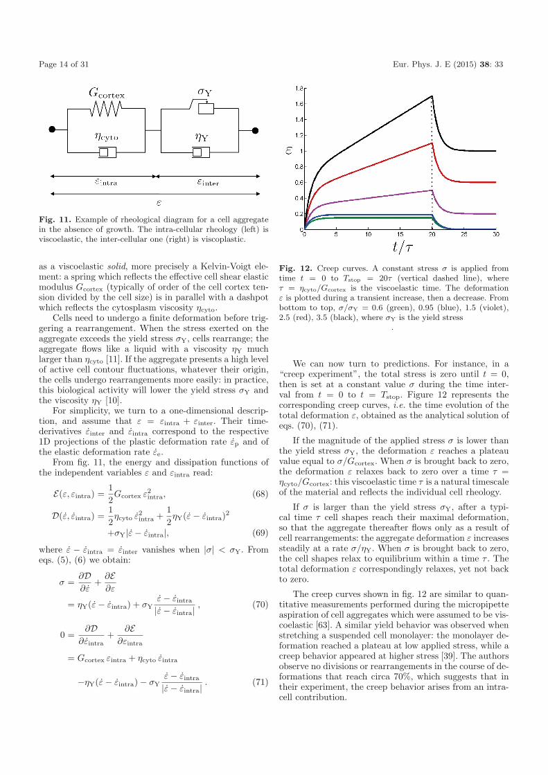
Fig. 11. Example of rheological diagram for a cell aggregatein the absence of growth. The intra-cellular rheology (left) isviscoelastic, the inter-cellular one (right) is viscoplastic.

as a viscoelastic solid, more precisely a Kelvin-Voigt ele-ment: a spring which reflects the effective cell shear elasticmodulus Gcortex (typically of order of the cell cortex ten-sion divided by the cell size) is in parallel with a dashpotwhich reflects the cytosplasm viscosity ηcyto.

Cells need to undergo a finite deformation before trig-gering a rearrangement. When the stress exerted on theaggregate exceeds the yield stress σY, cells rearrange; theaggregate flows like a liquid with a viscosity ηY muchlarger than ηcyto [11]. If the aggregate presents a high levelof active cell contour fluctuations, whatever their origin,the cells undergo rearrangements more easily: in practice,this biological activity will lower the yield stress σY andthe viscosity ηY [10].

For simplicity, we turn to a one-dimensional descrip-tion, and assume that ε = εintra + εinter. Their time-derivatives εinter and εintra correspond to the respective1D projections of the plastic deformation rate εp and ofthe elastic deformation rate εe.

From fig. 11, the energy and dissipation functions ofthe independent variables ε and εintra read:

E(ε, εintra) =12Gcortex ε2

intra, (68)

D(ε, εintra) =12ηcyto ε2

intra +12ηY(ε − εintra)2

+σY|ε − εintra|, (69)

where ε − εintra = εinter vanishes when |σ| < σY. Fromeqs. (5), (6) we obtain:

σ =∂D∂ε

+∂E∂ε

= ηY(ε − εintra) + σYε − εintra

|ε − εintra|, (70)

0 =∂D

∂εintra+

∂E∂εintra

= Gcortex εintra + ηcyto εintra

−ηY(ε − εintra) − σYε − εintra

|ε − εintra|. (71)

Fig. 12. Creep curves. A constant stress σ is applied fromtime t = 0 to Tstop = 20τ (vertical dashed line), whereτ = ηcyto/Gcortex is the viscoelastic time. The deformationε is plotted during a transient increase, then a decrease. Frombottom to top, σ/σY = 0.6 (green), 0.95 (blue), 1.5 (violet),2.5 (red), 3.5 (black), where σY is the yield stress

.

We can now turn to predictions. For instance, in a“creep experiment”, the total stress is zero until t = 0,then is set at a constant value σ during the time inter-val from t = 0 to t = Tstop. Figure 12 represents thecorresponding creep curves, i.e. the time evolution of thetotal deformation ε, obtained as the analytical solution ofeqs. (70), (71).

If the magnitude of the applied stress σ is lower thanthe yield stress σY, the deformation ε reaches a plateauvalue equal to σ/Gcortex. When σ is brought back to zero,the deformation ε relaxes back to zero over a time τ =ηcyto/Gcortex: this viscoelastic time τ is a natural timescaleof the material and reflects the individual cell rheology.

If σ is larger than the yield stress σY, after a typi-cal time τ cell shapes reach their maximal deformation,so that the aggregate thereafter flows only as a result ofcell rearrangements: the aggregate deformation ε increasessteadily at a rate σ/ηY. When σ is brought back to zero,the cell shapes relax to equilibrium within a time τ . Thetotal deformation ε correspondingly relaxes, yet not backto zero.

The creep curves shown in fig. 12 are similar to quan-titative measurements performed during the micropipetteaspiration of cell aggregates which were assumed to be vis-coelastic [63]. A similar yield behavior was observed whenstretching a suspended cell monolayer: the monolayer de-formation reached a plateau at low applied stress, while acreep behavior appeared at higher stress [39]. The authorsobserve no divisions or rearrangements in the course of de-formations that reach circa 70%, which suggests that intheir experiment, the creep behavior arises from an intra-cell contribution.

Eur. Phys. J. E (2015) 38: 33 of 31

Fig. 13. Sketch of a cell aggregate confined between parallelplates [107], a distance h apart. The size L increases with timedue to cell division cycles.

4.2 With divisions: inhomogeneous proliferation

When the duration of the experiment becomes muchlonger than r−1

cc , cell divisions must be taken into accountand the aggregate flows even under a weak stress [9].

Figure 13 represents an experiment [107] where a cellaggregate is confined between parallel rigid plates. Theaggregate length L(t) grows from initially L0 ∼ 400μmto LT ∼ 700μm in T = 3 days and LT ∼ 1200μmin T = 6 days. We thus estimate the growth rate asαg ≈ 2 log(LT /L0)/T � 4.2 · 10−6 s−1, where the factor 2reflects the fact that growth occurs effectively in only twodimensions: cells divide mostly at the aggregate periph-ery. The main hypothesis proposed by [107] is that thestress induced by growth in the confined aggregate couldmechanically inhibit mitosis.

4.2.1 Model with divisions

We propose to qualitatively model the aggregate growthcoupled to its mechanical response (determined insect. 4.1). Assuming translational invariance along z, wetreat this problem in the xy plane (d = 2). We introduceseparate rheological diagrams for the trace and the devi-ator.

According to the mass conservation (eq. (24)), thetrace tr ε of the deformation rate is equal to the growthrate αg of the aggregate. Within a linear approxima-tion [12], we assume that αg decreases with the pressureP = − tr σ/d, from its value εg at zero pressure, as

αg = εg

(1 +

tr σ

Pgd

), (72)

where we use the pressure Pg actively generated by theaggregate at zero deformation rate, e.g. when confined be-tween fixed walls. We deduce the rheological equation forthe trace (fig. 14, top part)

tr ε = εg +tr σ

ηg, (73)

where we define an effective growth-induced viscosity co-efficient ηg [12]

ηg =Pgd

εg, (74)

which differs from the effective division-induced viscositycoefficient

ηcc =G

rcc, (75)

Fig. 14. Rheological diagrams for the trace (top) and the de-viator (bottom) of the stress in a cell aggregate in the presenceof growth. Here εg is the aggregate growth rate at zero pressureand ηg quantifies the influence of pressure on aggregate growth(eq. (74)), G is the effective cell shear elastic modulus, ηcyto

the single cell viscosity, ηcc the aggregate viscosity related todivisions.

where rcc is the division rate.We further assume that deviatoric stresses generated

by the growth are lower than the yield stress σY. On theother hand, here (as opposed to sect. 4.1), we considertime scales which are long enough (compared with the celldivision cycle) that the aggregate viscosity ηcc related tocell divisions is now relevant. The inter-cellular viscoplas-tic element of fig. 11 is replaced by a dashpot (fig. 14,bottom).

The energy and dissipation functions for these dia-grams read

E(dev εintra) =12G(dev εintra)2, (76)

D(tr ε,dev ε, dev εintra) =12ηg(tr ε − εg)2

+12ηcyto(dev εintra)2 +

12ηcc(dev ε − dev εintra)2. (77)

Considering dev εintra, tr ε, dev ε and dev εintra asindependent variables and using eqs. (B.10)-(B.13),eqs. (76), (77) yield

tr σ = ηg(tr ε − εg), (78)dev σ = ηcc(dev ε − dev εintra), (79)

0 = G dev εintra + ηcyto dev εintra

+ ηcc(dev εintra − dev ε). (80)

Finally, using a few substitutions to eliminate dev εintra

and dev εintra between eqs. (79)-(80), we obtain(

1 +ηcyto

ηcc

)dev σ +

dev σ

τcc= ηcyto dev ε + Gdev ε, (81)

where τcc ≈ ηcc/G = r−1cc is a viscoelastic relaxation time

associated with cell division cycles.

of 31 Eur. Phys. J. E (2015) 38: 33

Provided gravity and other body forces are negligible,the stress is divergence-free in the bulk of the aggregate

∂xσxx + ∂yσxy = 0, (82)∂yσyy + ∂xσxy = 0. (83)

4.2.2 Symmetries

Equations (78)-(83) can be simplified as follows. We as-sume (and check a posteriori) that internal forces aremuch larger than inertial terms in eq. (13), which thusreduces to eq. (14). Furthermore, the plates are rigid andimmobile: we can safely assume that the vertical compo-nent vy of the velocity is equal to zero not only at theplates, but also in the whole aggregate (that condition ispossibly violated within a small edge region, of width com-parable to the thickness h). As a consequence, the verticalcomponent of the deformation rate, εyy, is identically zero.

Further simplifications result from the symmetry ofthe aggregate both in direction x along the length and indirection y across the thickness. Some quantities are evenfunctions of the y-coordinate, namely the horizontal veloc-ity vx and the horizontal component εxx of the deforma-tion rate, stress components σxx and σyy aligned with theplates, and y-derivatives of odd functions, such as ∂yσxy.Other quantities are odd functions of y, for instance shearcomponents of the stress σxy and of the deformation rateεxy, x-derivatives of other odd functions such as ∂xσxy,and y-derivatives of even functions such as ∂yvx or ∂yσyy.

As a result, after averaging along y, the deformationrate has only one non-zero component εxx; the deviatoricstress has only diagonal terms and thus only one indepen-dent component, say (σxx − σyy)/2.

With these simplifications, eqs. (78)-(82) become

σxx + σyy = ηg(εxx − εg), (84)(

1 +ηcyto

ηcc

)(σxx − σyy)

+σxx − σyy

τcc= ηcytoεxx + Gεxx, (85)

∂xσxx = − 2h

σxy|y=h/2 . (86)

We now assume that ηcyto ηcc ηg, based onthe following orders of magnitude. Single cell viscosityηcyto is around 102 Pa s [108]. Aggregate viscosity ηcc

extracted from cell aggregates fusion and aspiration isaround 105 Pa s [63,109]. Using data of cell aggregategrowth under pressure [12], a value of ηg around 109 Pa shas been proposed [110]. Encapsulated growing aggregateswhich deform a capsule yield a value Pg ∼ 2000Pa [43],where a dramatic decrease of the aggregate growth is ob-served. Taking εg ∼ 5 · 10−6 s−1 yields ηg around 109 Pa s,consistent with the previous estimation.

4.2.3 Boundary conditions

Equations (84)-(86) must be complemented with the freeedge boundary condition

σxx|x=±L/2 = 0. (87)

Let us first assume that we could neglect the friction ofhorizontal plates, σxy|y=±h/2 = 0. Then eq. (86) and theedge boundary condition (eq. (87)) would imply a vanish-ing horizontal stress in the whole aggregate: σxx(x) = 0.Under these conditions, eqs. (84)-(85) would predict thatafter a transient time of order τcc, the vertical stress andthe horizontal deformation rate would reach a stationaryvalue: σyy → −ηccεg and εxx → εg. Hence, an exponentialincrease of the aggregate size L(t) ∼ exp(εg t) would beexpected, with a spatially uniform proliferation, at oddswith the experimental observation that cells divide onlyat the aggregate periphery.

This is why we do explicitly take into account the fric-tion on plates. In a linear approximation, the friction canbe assumed proportional to the local aggregate velocity

σxy

(x,

h

2

)= −ζvx

(x,

h

2

). (88)

Under the assumption ηcyto ηcc, eq. (81) implies σxy �ηcc∂yvx. Hence, if we assume that the friction coefficient ζis small enough that we can neglect the velocity variationsacross the aggregate thickness |h ∂yvx/vx| � h ζ/ηcc, thevelocity profile is approximately a plug flow: vx(x, h/2) ≈vx(x). Combining eqs. (86), (88) and the relation εxx =∂xvx (eq. (11)), yields

vx =h

2ζ∂xσxx, (89)

εxx =h

2ζ∂2

xσxx. (90)

Within the approximation ηcyto ηcc ηg, combiningeqs. (84), (85), (90) so as to eliminate σyy yields an evo-lution equation for the horizontal component of the stress

τccσxx + σxx = −Pg + τccλ2∂2

xσxx + λ2∂2xσxx,

where the characteristic length λ is

λ =

√ηgh

4ζ, (91)

while σyy passively follows σxx according to

σyy = −σxx + 2λ2 ∂2xσxx − 2Pg. (92)

The motion of the aggregate edge results from the velocity:12 L(t) = vx(L/2, t). From eqs. (87), (89), the boundaryconditions are

σxx

(−L

2, t

)= σxx

(L

2, t

)= 0, (93)

h

ζ∂xσxx

(L

2

)= L. (94)

Eur. Phys. J. E (2015) 38: 33 of 31

4.3 Resolution

4.3.1 Change of variables

We introduce the rescaled variables X = 2xL(t) , Σ(X, t) =

σxx(x, t), Λ(t) = 2λL(t) and the new function

F (X, t) = Σ − Λ2(t)∂2XΣ + Pg. (95)

Equation (91) becomes

τcc∂tF + F =τccXL(t)

L(t)∂XF. (96)

The boundary conditions (eqs. (93), (94)) read:

Σxx(−1, t) = Σxx(1, t) = 0, (97)2h

ζL(t)∂XΣxx(1, t) = L. (98)

Equation (96) can be further rewritten in terms ofthe variable Z = log X and the function K(Z, t) =exp(t/τcc)F (X, t)

∂tK(Z, t) − L(t)L(t)

∂ZK(Z, t) = 0. (99)

4.3.2 Initial conditions

Just before the first time of contact between the aggre-gate and the walls, the cells constituting the aggregate donot undergo any elastic deformation. Thus dev εintra(t =0−) = 0. The cell deformation is continuous in time, sodev εintra(t = 0+) = 0. From this condition and eq. (80),we obtain:

dev εintra(x, 0+) =ηcc

ηcc + ηcytodev ε(x, 0+). (100)

Substituting eq. (100) into eq. (79), and eliminating σyy

with eq. (78), we obtain

2σxx(x, 0+) =(

ηg +ηccηcyto

ηcc + ηcyto

)εxx(x, 0+) − ηgεg.

(101)Using again ηcyto ηcc ηg and eq. (90), we obtain

σxx(x, 0+) − λ2∂2xσxx(x, 0+) = −Pg. (102)

4.3.3 Analytical solution

Solving eq. (99) with the boundary conditions ofeqs. (97), (98) and the initial condition of eq. (102) yieldsthe following analytical solution, in terms of the initialvariables:

L

2λ= sinh−1

(eεgt sinh

L0

2λ

), (103)

σxx = Pg

[cosh x

λ

cosh L(t)2λ

− 1

]. (104)

Equation (89) then yields

vx

(L

2, t

)=

hPg

2ζ λtanh

L

2λ, (105)

while eq. (92) yields

σyy = σxx (106)

and from eqs. (104), (106), the pressure is

P = −σxx + σyy

2

= Pg

[1 −

cosh xλ

cosh L(t)2λ

]. (107)

4.3.4 Discussion

Equation (103) shows that as long as L(t) 2λ, the ag-gregate growth rate is L(t) ≈ εgL(t). The aggregate lengthincreases with time as L(t) ≈ L(0) exp(εgt), as it wouldbe in the absence of friction (sect. 4.2.3).

For L(t) 2λ, the aggregate growth rate is L(t) ≈2εgλ. The aggregate grows linearly in time as L(t) ≈2εgλt. The growth is localized in a zone of typical sizeλ at the border of the aggregate. After a transient regimewhich lasts of the order of τcc, the pressure decreases ex-ponentially on a lengthscale λ from 0 at the border of theaggregate to Pg inside the aggregate.

Since cell division can be affected by mechanicalstresses, this model could explain why cell divisions areinhibited inside the confined growing aggregate, except ina region of width λ [107]. Since the pressure affects thegrowth rate, which in turn affects ηcc, the model could beextended to include the spatial variation of ηcc: the pres-sure would be expected to increase dramatically in theinner part of the aggregate.

The length λ defined in eq. (91) increases as the squareroot of h: this could be checked experimentally by chang-ing h. The pressure profile predicted by eq. (107), plottedin fig. 15, could be checked by looking at aggregates grow-ing between deformable plates.

We can estimate a posteriori orders of magnitude inexperiments [107]. From the width of the proliferating re-gion, we estimate λ to be of order of 10−4 m. Velocitiesare of order 1

2αgL, i.e. a few 10−10 ms−1. Based on a typ-ical value of the effective viscosity ηg ∼ 109 Pa s [12] andthe growth rate αg, the stationnary value of pressure Pg

in the aggregate is estimated as a few 103 Pa. The iner-tial terms in eq. (13) are respectively ρ ∂tv ∼ ρv/T andρ v∇v ∼ ρv2/λ, both of order of a few 10−13 Nm−3: theyare much smaller than the other terms, for instance thedivergence of the stress ∇ · σ which is of order of Pg/λ,namely a few 107 Nm−3.

When confining plates are removed, the aggregateshape relaxes first quickly, then more slowly towards asphere [10,107]. The fast relaxation is over the time scaleof minutes whereas the slower one is over many hours. The

of 31 Eur. Phys. J. E (2015) 38: 33

Fig. 15. Space dependence of the pressure in the confinedgrowing aggregate, at different times (eq. (107)). Parame-ters (see text): τcc = 8 h, λ = 100 μm, εg = 5.10−6 s−1,Pg = 2000 Pa.

fast relaxation could correspond to the relaxation of theelastic deformation of individual cells generated by con-fined growth, where the driving force is dominated by thecell elasticity rather than surface tension, and the dissipa-tion dominated by the intra-cellular viscosity. Conversely,the slow relaxation phase could correspond to the round-ing of the aggregate under surface tension after the relax-ation of stored elasticity. Measuring the relaxation ampli-tude as a function of the position in the aggregate couldbe a way to estimate the spatial profile of the deviatoricstress generated by growth.

5 Conclusion

When modelling the mechanical behaviour of living tis-sues, it is important to be able to build a sensible rheo-logical model and to derive the corresponding dynamicalequations in a systematic manner. We present here a tool-box to model the mechanics underlying the morphogenesisof tissues whose mechanical behaviour is that of a contin-uous material. Once a given problem has been analysed indetails and appropriately simplified, this toolbox shouldenable to incorporate into models large amounts of dataregarding feedbacks between genetics and mechanics.

We have suggested to proceed in four steps. First, tolist the relevant ingredients, classified into intra-cell mech-anisms (cell elasticity and relaxation, cell growth, cell con-tractility) and inter-cell mechanisms (rearrangements, di-vision and apoptosis), which affect the tissue shape and/orvolume. Second, to combine the mechanical ingredientsinto rheological diagrams. Third, to translate such dia-grams into the dissipation function formalism, taking intoaccount couplings with non-mechanical fields. Fourth, toderive a set of partial differential equations to be solved.

Section 5.1 discusses the dissipation function for-malism. Section 5.2 examines possible applications. Sec-tion 5.3 opens perspectives.

5.1 Dissipation function formalism

The dissipation function formalism has the following lim-itations. It can include only a subclass of all conceivablemechanical or biological ingredients. It obeys the Onsagersymmetry theorem only when fluxes and forces behavesimilarly under time reversal.

Conversely, the dissipation function formalism has thefollowing advantages. It is a convenient tool for buildingcomplex models and obtaining in an automatic way thefull set of partial differential equations which respect ten-sorial symmetry in any dimensions. It includes and gener-alizes the rheological diagram formalism and the hydrody-namic formalism. For tissues with non-mechanical ingredi-ents, it allows to systematically explore possible couplings.Its coupling coefficients arise as cross partial derivatives,thus derive from a smaller number of free parameters thanin the hydrodynamics formalism. It is suitable for nonlin-ear terms, whether analytic or not, including terms domi-nant over linear terms, like plasticity. In the case of smalldeformations, the convexity of the energy and dissipationfunctions warrants that there exists a unique solution, andthat it satisfies the second law of thermodynamics. Nu-merically, it allows to use a variational approach, whichmakes it useful for the resolution of the dynamical equa-tions. In view of these advantages, we recommend to adoptthe dissipation function formalism for models of living tis-sues within continuum material mechanics.

A complete set of partial differential equations mod-elling the tissue can be explicitly derived from the energyand dissipation functions, using the method described insect. 2.2.3 and appendix B, and can be solved numerically.Ingredients specific to living tissues, such as cell contrac-tility or growth, can be included in a consistent manner asshown in sect. 3, which includes both simple and complexexamples. An example is fully solved in sect. 4.

5.2 Practical applications

Tools exist to analyse 2D or 3D movies of tissue dy-namics and perform quantitative measurements within acontinuum mechanics description. Data can be comparedwith the model predictions, i.e. numerical solutions of themodel equations. Such a comparison is instrumental in de-termining the values of the unknown parameters, and isindeed already possible on a large scale in both animaland vegetal tissues.

To constrain the models, it is essential to limit thenumber of mechanical parameters, which should be muchlower than the number of measurements available. In thisrespect, the continuum description is more economicalthan a simulation of a whole tissue at the cell scale. Thisadvantage may be crucial when, e.g., studying feedbacksbetween gene expression and mechanical response. In situmeasurements of local force and stress are improving at aquick pace and will hopefully be soon compared with lo-cal elastic deformation measurements. Our modelling ap-proach should help exploit the future wealth of availabledata and incorporate it into a consistent picture.

Eur. Phys. J. E (2015) 38: 33 of 31

In principle, the present approach should be relevant todynamically evolving assemblies of cohesive cells such asencountered in animal tissues during development, woundhealing, tumorigenesis, as well as in in vitro aggregates.In other types of tissues, we expect some of the presentingredients to be irrelevant. In an adult tissue withoutany significant chemical or mechanical stress, cell divi-sion and rearrangements can become negligible. In a tis-sue where cell divisions and apoptoses are negligible andwhere a strong cell-cell adhesion or an extra-cellular ma-trix hinders plasticity, we expect the tissue rheology toessentially reflect the single cell behaviour. The presentapproach should thus remain relevant, provided some ofthe parameters are taken as zero.

5.3 Perspectives

Different issues need to be overcome in order to validatecontinuum descriptions of tissues from experimental data.First, an adequate averaging procedure should be chosen.An optimal length scale of measurement must be prop-erly defined, larger that the typical cell size, but smallerthan the sample size, and therefore suitable for hydrody-namics. Averages over time or over an ensemble of ex-periments performed in identical conditions may improvethe signal-to-noise ratio. A second difficulty originates inthe large size of data, in terms of manipulation and rep-resentation. Third, the formalism of generalised standardmaterials, initially developed for hard condensed matter,will probably require specific modelling efforts to incor-porate features of soft condensed matter and biophysics,such as progressive onset of plasticity due to cell contourfluctuations, two-phase coexistence corresponding to mul-tiple minima in the energy or dissipation functions, ordeformation-dependent terms in the dissipation function.

Facing this task, it is important to determine the bestapproach in representing and correlating various fields, inorder to obtain a more intuitive grasp of the relative im-portance of various couplings. Quite generally, genetic en-gineering or pharmacological treatment can help discrimi-nate the contribution made by a particular ingredient. Forinstance, computing the differences between wild-type tis-sues and mutants enables to delineate separately the con-tribution of a single ingredient within a complex feedbacknetwork, and to further validate a model.

In the more distant perspective of integrating ingre-dients from genetics with mechanical models to fully un-derstand morphogenetic processes, some questions shouldbe considered. What kind of model parameters can beextracted from state-of-the art experimental data? Whatminimal set of data is required to extract the parametersassociated with a given class of models? Or reciprocally,given a modelling framework, what set of minimal exper-iments are necessary for validation and parameter extrac-tion? Can we discriminate among models on the basis oftheir capacity to interpret the data in the most economicalway?

It is a pleasure to thank Isabelle Bonnet, Ibrahim Ched-dadi, Helene Delanoe-Ayari, Guillaume Gregoire, Shuji Ishi-hara, Pierre Recho, Jean-Francois Rupprecht for a critical read-ing of the manuscript.

Appendix A. From discrete cells to tissuescale

Tools are required to link the scale of discrete cells withthe global scale of the tissue treated as a continuous ma-terial. Appendix A.1 presents tensorial tools to describecellular materials. Appendix A.2 focuses on the particularquestion of size and growth. Appendix A.3 incorporatesgrowth in the dynamics, treated as a scalar for simplicity.

Appendix A.1. Tensorial tools to describe cellularmaterials

This appendix presents some descriptive tensors. They canbe measured visually without any knowledge of either thephysics or the biology that determine the tissue behaviour,nor of the past history of the tissue. These tensors arecalled static (respectively, kinematic) when they can bedetermined from still images (respectively, movies).

Blanchard et al. [111,112] measure separately the de-formation rate and the cell shape changes. Their differenceis attributed only to the net effect of cell rearrangements,which is thus indirectly estimated.

These measurements can be unified using the tex-ture tensor, which enables a direct and independent mea-surement of the deformation rate, the cell shape changesand the rate of rearrangements [68]. Briefly, considertwo cells which share an edge (fig. 16). In the 2D case,their centers of mass have coordinates r1 = (x1, y1) andr2 = (x2, y2). A pair of such cells is called a “link”, char-acterised by the vector � = r2 − r1 with coordinates(X,Y ) = (x2 − x1, y2 − y1). The link vector carries theinformation on link length and angle. The link matrix mis defined as:

m = � ⊗ � = � �T =(

X2 XY

Y X Y 2

). (A.1)

It retains the information of link size and angle, but notof its sign. This measurement becomes multi-scale uponcoarse-graining over some spatial domain, by performingaverages over several links (fig. 16c); time averages overseveral images can be performed too. Averaging m overa group of cells, at any chosen length and/or time scale,reduces the whole cell pattern to the information of defor-mation and anisotropy over the corresponding set of links,called its texture, M = 〈m〉:

M = 〈� ⊗ �〉 = 〈� �T 〉 =( 〈X2〉〈XY 〉〈Y X〉〈Y 2〉

). (A.2)

There exist two orthogonal axes (eigenvectors) in whichM would be diagonal, with strictly positive eigenvalues

of 31 Eur. Phys. J. E (2015) 38: 33

Fig. 16. Measurement of texture. (a) Snapshot of a foam, in anisotropic region; its texture has two equal eigenvalues. Straightlines, called “links”, are drawn between centers of neighbouringcells. (b) Same foam, in an anisotropic region; its texture hastwo different eigenvalues. (c) A tissue. Links are drawn over awhole region. Reprinted from [68].

λi (i = 1 or 2), of order of link mean square length ineither direction. M is represented by an ellipse with axesproportional to the eigenvalues λi. It is more circular infig. 16a than in fig. 16b.

Kinematic tensors such as the deformation rate, thecell shape changes and the rate of rearrangements can beexpressed using the formalism based on this texture [68].The cell shape changes correspond to the changes in tex-ture. The links which appear (or disappear) in the timeinterval between two successive images of a movie char-acterise changes in the cell pattern topology and can becombined to measure the rearrangement rate contributionto the inter-cell deformation rate, εinter. All links which areconserved during the time interval between two successiveimages of a movie can be tracked: their changes expressthe relative motion of pairs of neighboring cells, and thusmeasure the velocity gradient, ε.

Appendix A.2. Volume

We show here that the average cell volume is related tothe determinant of tensor M and use it to estimate thegrowth rate αg from local measurements.

In 2D, let �1, �2 and �3 be link vectors between threeneighbouring cell centers. One can show that

(�1 × �2)2 + (�2 × �3)2 + (�3 × �1)2

= det(�1 ⊗ �1 + �2 ⊗ �2 + �3 ⊗ �3). (A.3)

Fig. 17. Notations for the discrete approach of growth. A one-dimensional tissue of length L is made of N cells of length �.

Hence, the surface area of the triangle, S123 = 12 |�1 × �2|,

can be expressed as

S123 =1

2√

3

√det(�1 ⊗ �1 + �2 ⊗ �2 + �3 ⊗ �3) . (A.4)

In a large two-dimensional assembly, the number of suchtriangles is equal to twice the number of cell centers [72].Hence, the average surface area per cell is

〈Scell〉 ≈ 2 〈S123〉

=1√3〈√

det(�1 ⊗ �1 + �2 ⊗ �2 + �3 ⊗ �3)〉

≈√

3 det(M) . (A.5)

In 3D, a similar relation holds for the cell volume

〈Vcell〉 ∝√

det(M) . (A.6)

Hence, both in 2D and 3D, the growth rate αg is ap-proximately:

αg ≈ 12 det M

d(det M)dt

. (A.7)

Note that eq. (A.7) becomes exact when M is replacedby the similar tensor B [69]. It relates vectors �0 locatedon a circle in the relaxed configuration with vectors � onan ellipse in the current configuration (�T B−1� = �T

0 �0),so that B = I in a relaxed configuration, where I denotesthe unit tensor.

Appendix A.3. Growth: discrete and continuousdescriptions

In the present appendix, we derive and interpret eq. (32).We discuss how to start from a discrete description of theeffect of growth in the tissue, to derive the correspondingcontinuum description, first in kinematics, then in dynam-ics. For simplicity, we treat here a one-dimensional tissueof length L, made of N cells of same length �, mass m,spring constant K and rest length �0 (fig. 17):

L = N�. (A.8)

Appendix A.3.1. Kinematics

The tissue mass is M = Nm, and the growth rate αg

obeysdN

dt= αg N . (A.9)

Eur. Phys. J. E (2015) 38: 33 of 31

Meanwhile, the Eulerian elongation rate ε (eq. (11)) obeys

dL

dt= εL . (A.10)

Differentiating eq. (A.8) with respect to time and usingeqs. (A.9), (A.10) yields the time evolution of the celllength �

1�

d�

dt= ε − αg . (A.11)

The cell elongation rate is thus the difference between thetissue elongation rate and the growth rate.

Appendix A.3.2. Dynamics

Within the limit of small elastic deformations, the cellelongation �−�0 determines the stress σ and the elasticallystored part of the deformation

σ = K (� − �0), (A.12)

εe =� − �0

�0. (A.13)

Combining eq. (A.11) with eq. (A.13) yields

εe = (ε − αg)�

�0= (1 + εe)(ε − αg) (A.14)

so that, still in the limit of small deformations

εe � ε − αg. (A.15)

Injecting eqs. (A.12), (A.13) into the continuum elasticityeq. (34) yields the elastic modulus of a tissue

G ≡ K �0 (A.16)

which, combined with eq. (A.15), yields the stress evolu-tion eq. (32).

At large deformations (see appendix D), eq. (A.13)admits several possible generalisations, see for instanceeq. (D.17), each of which in turn yields a slightly differentversion of eq. (A.15), and thus of eq. (32).

Appendix B. Rheological diagrams anddissipation function

Within the dissipation function formalism, appendix B.1explains how to derive equations when starting from a rhe-ological diagram. Appendix B.2 explicits calculations fortensors, while appendix B.3 examines their incompressiblecase. Appendix B.4 shows recursively that any rheologicaldiagram can be included, whatever its complexity.

Appendix B.1. Deriving equations

This appendix retraces practical calculations on a simpleexample. It shows that the formalism of eqs. (3)-(6) withm = 1 can describe the diagram discussed in sect. 2.2.1,yielding eq. (2).

When conducting explicitly the calculations outlinedin sect. 2.2.3, there are redundant variables. They can beeliminated by taking into accoung the topological relationsof the diagram. For instance, the diagram represented infig. 1 involves three different deformation rates which arenot independent: ε, ε1 and ε2. A naive formulation of theenergy and dissipation functions would read

E =12G1ε

21, (B.1)

D =12η1ε

22 +

12η2ε

2. (B.2)

The topology of the diagram provides the relationship be-tween the deformation variables

ε = ε1 + ε2, (B.3)ε = ε1 + ε2. (B.4)

Note that in the dissipation function formalism, internalvariables must be independent. Each spring should be as-sociated with one of the chosen, independent variables,such as ε1. Equations (B.3), (B.4) enable to drop one ofthe internal variables, for instance ε2

E (ε, ε1) =12G1ε

21, (B.5)

D (ε, ε1) =12η1 (ε − ε1)

2 +12η2ε

2. (B.6)

Equations (5), (6) with m = 1 yield

σ = η1 (ε − ε1) + η2ε, (B.7)0 = G1ε1 + η1 (ε1 − ε) . (B.8)

Eliminating ε1 and ε1 between eqs. (B.7), (B.8) indeedyields eq. (2).

Appendix B.2. Tensorial case and example

This appendix generalizes the explicit calculations ofsect. B.1 to a tensorial case and provides an example.The large deformation case is treated in appendices D.2.3and D.2.4.

It is convenient to decompose each deformation tensor,such as ε, into two independent parts: an isotropic partwhich alters the volume and is proportional to the tracetr ε of the tensor, and an anisotropic part which affectsthe shape and is the tensor deviator dev ε = ε − 1

d tr εI

ε =1d

tr ε I + dev ε , (B.9)

where I denotes the unit tensor.

of 31 Eur. Phys. J. E (2015) 38: 33

Fig. 18. A Maxwell viscoelastic liquid.

Since the deformation ε is now split into two indepen-dent variables tr ε and dev ε, the expression of the stress(eq. (5)) must be reconsidered. Since E and D are scalars,the expression derived through differentiation with respectto dev ε and dev ε is also a traceless tensor. It is thus nat-urally identified with dev σ

dev σ =∂D

∂ dev ε+

∂E∂ dev ε

. (B.10)

Finally, the corresponding expression with traces is ascalar and is identified with trσ

tr σ =∂D

∂ tr ε+

∂E∂ tr ε

. (B.11)

The same decomposition, applied to eq. (6), yields

0 =∂D

∂ dev εk+

∂E∂ dev εk

, (B.12)

0 =∂D

∂ tr εk+

∂E∂ tr εk

. (B.13)

As an example, we choose for simplicity to treat aMaxwell viscoelastic liquid (fig. 18, equivalent to fig. 1with η2 = 0). In the compressible case, the stress is thesum of the following elastic and viscous contributions de-limited by square brackets:

σ = [2Gdev ε1 + K tr ε1 I]+ [2η (dev ε − dev ε1) + χ (tr ε − tr ε1) I] . (B.14)

The constitutive equation (B.14) can be decomposed intotrace and deviator, which in the present example yields

tr σ = χ d (tr ε − tr ε1), (B.15)dev σ = 2η (dev ε − dev ε1), (B.16)

0 = K d tr ε1 + χ d (tr ε1 − tr ε), (B.17)0 = 2Gdev ε1 + 2η (dev ε1 − dev ε). (B.18)

Coming back to energy and dissipation functions, traceand deviatoric components can be considered as indepen-dent variables

E = G (dev ε1)2 +12K (tr ε1)2, (B.19)

D = η (dev ε − dev ε1)2 +12χ (tr ε − tr ε1)2. (B.20)

Using eqs. (B.10)-(B.13) with eqs. (B.19)-(B.20) yieldseqs. (B.15)-(B.18), as expected.

Appendix B.3. Incompressible case

The incompressible limit occurs when the parameters Kand χ go to infinity while the stress remains finite. Thedegrees of freedom for volume change represented by thetrace of the deformations and deformation rates are frozen.They should therefore be absent from the energy and dis-sipation expressions, and trσ is undetermined.

In the case of a Maxwell viscoelastic liquid (fig. 18),eqs. (B.19), (B.20) for the energy and dissipation functionsbecome

E = G (dev ε1)2, (B.21)

D = η (dev ε − dev ε1)2. (B.22)

Using eqs. (B.10)-(B.13), the resulting equations are iden-tical to eqs. (B.16), (B.18):

dev σ = 2η (dev ε − dev ε1), (B.23)0 = 2Gdev ε1 + 2η (dev ε1 − dev ε). (B.24)

Appendix B.4. Recursive construction of dissipationfunction

We show here that any rheological diagram can be de-scribed within the dissipation function formalism. Thebasic ingredients (e.g. a dashpot, a slider, a viscoelasticelement, etc.) have been studied in the main text, partic-ularly in sect. 3, and successfully described within the dis-sipation function formalism. An arbitrarily complex rhe-ological diagram can be generated by successive combi-nations, either in parallel or in series, of simpler subdi-agrams. We need to prove recursively that constitutiveequations obtained directly from an arbitrary rheologicaldiagram are identical to those obtained from eqs. (5), (6)within the dissipation function formalism.

Let Sα be a first subdiagram with total deformationεα, total deformation rate εα, mα internal variables εk

(1 ≤ k ≤ mα), a free energy Eα(εα, ε1, . . . , εmα) and a dis-

sipation function Dα(εα, ε1, . . . , εmα). Then eqs. (3), (4)

write

σα =∂Dα

∂εα+

∂Eα

∂εα, (B.25)

0 =∂Dα

∂εk+

∂Eα

∂εk, 1 ≤ k ≤ mα, (B.26)

where σα denotes the stress of subdiagram Sα. Similarly,a second subdiagram Sβ is defined with mβ internal vari-ables, and constitutive equations given by

σβ =∂Dβ

∂εβ+

∂Eβ

∂εβ, (B.27)

0 =∂Dβ

∂εk+

∂Eβ

∂εk, mα + 1 ≤ k ≤ mα + mβ . (B.28)

The total free energy and dissipation functions of the com-bined diagram S = Sα ∪ Sβ are formally defined as

E = Eα + Eβ , (B.29)D = Dα + Dβ . (B.30)

Eur. Phys. J. E (2015) 38: 33 of 31

Fig. 19. Two subdiagrams Sα and Sβ in parallel (left) andin series (right) with their respective deformations εα, εβ andstresses σα, σβ .

The next sections show that when Sα and Sβ are combinedeither in parallel (sect. B.4.1) or in series (sect. B.4.2), aproper choice of independent variables for E and D yieldsthe expected constitutive equations for S

σ =∂D∂ε

+∂E∂ε

, (B.31)

0 =∂D∂εk

+∂E∂εk

, (B.32)

in agreement with the mechanical equations relating σ toσα, σβ , and ε to εα, εβ (fig. 19).

Appendix B.4.1. Two subdiagrams in parallel

We consider here the combination in parallel of Sα andSβ , with identical deformation and deformation rate (seefig. 19, left)

ε = εα = εβ , (B.33)ε = εα = εβ . (B.34)

Here, Sα and Sβ can be decoupled or coupled.We first examine the case where Sα and Sβ are de-

coupled (no duplicate internal variables). This is the casefor subdiagrams composed of mechanical elements only:all internal variables pertaining to Sα are distinct from allinternal variables pertaining to Sβ . The energy and dis-sipation functions depend on the following independentvariables:

E = E(ε, ε1, . . . , εmα+mβ), (B.35)

D = D(ε, ε1, . . . , εmα+mβ). (B.36)

Equations (B.26), (B.28) yield eq. (B.32) for all inter-nal variables of S, 1 ≤ k ≤ mα + mβ . The expression forthe stress σ of the combined diagram S is correct

σ =∂D∂ε

+∂E∂ε

=(

∂Dα

∂ε+

∂Dβ

∂ε

)+

(∂Eα

∂ε+

∂Eβ

∂ε

)

=(

∂Dα

∂εα+

∂Dβ

∂εβ

)+

(∂Eα

∂εα+

∂Eβ

∂εβ

)

= σα + σβ . (B.37)

Second, we examine the case where Sα and Sβ are cou-pled. This is the case if non-mechanical internal variablescouple to mechanical internal variables of both Sα and Sβ .Duplicates must then be eliminated when selecting inde-pendent internal variables of S. For convenience, we orderinternal variables as:

Eα(εα, ε1, . . . , εp, εp+1, . . . , εmα),

Eβ(εβ , εmα+1, . . . , εmβ+p, εmβ+p+1, . . . , εmα+mβ),

with mα − (p+1) duplicate variables εk = εmβ+k, p+1 ≤k ≤ mα. Pruning redundant variables yields the followingchoice of independent variables for S

E(ε, ε1, . . . , εp, εp+1, . . . , εmα, εmα+1, . . . , εmβ+p),

D(ε, ε1, . . . , εp, εp+1, . . . , εmα, εmα+1, . . . , εmβ+p)

(compare with eqs. (B.35), (B.36)), while eq. (B.37) isunchanged, and we check that, for the initially redundantvariables, i.e., for p + 1 ≤ k ≤ mα

∂D∂εk

+∂E∂εk

=(

∂Dα

∂εk+

∂Eα

∂εk

)+

(∂Dβ

∂εmβ+k+

∂Eβ

∂εmβ+k

)

= 0 + 0= 0. (B.38)

Appendix B.4.2. Two subdiagrams in series

We consider here the combination in series of Sα and Sβ

(see fig. 19, right). Since

ε = εα + εβ , (B.39)ε = εα + εβ , (B.40)

we (arbitrarily) choose to keep εα and εα rather than εβ

and εβ as independent variables.In the absence of duplicate internal variables between

Sα and Sβ , we choose as independent variables

E(ε, ε1, . . . , εmα+mβ, εα),

D(ε, ε1, . . . , εmα+mβ, εα).

For 1 ≤ k ≤ mα (respectively, mα + 1 ≤ k ≤mβ), eq. (B.32) is identical to eq. (B.26) (respectively,eq. (B.28)).

We next consider the change of variables (εα, εβ) →(ε, εα), (εα, εβ) → (ε, εα). Since

∂

∂ε |εα

=∂

∂εβ |εα

,

∂

∂εα |ε=

∂

∂εα |εβ

− ∂

∂εβ |εα

(and similar expressions involving the rates of deforma-tion) we deduce

∂E∂ε |εα

=∂Eβ

∂εβ |εα

,

∂D∂ε |εα

=∂Dβ

∂εβ |εα

of 31 Eur. Phys. J. E (2015) 38: 33

andσ = σβ ,

using eqs. (B.27), (B.31). Further, since

∂E∂εα |ε

=∂Eα

∂εα |εβ

− ∂Eβ

∂εβ |εα

,

∂D∂εα |ε

=∂Dα

∂εα |εβ

− ∂Dβ

∂εβ |εα

,

we also have

σα − σβ =(

∂Dα

∂εα+

∂Eα

∂εα

)−

(∂Dβ

∂εβ+

∂Eβ

∂εβ

)

=∂D∂εα |ε

+∂E∂εα |ε

= 0, (B.41)

so that σα = σβ , in agreement with the rheological dia-gram (fig. 19, right).

If there are duplicate internal variables, they can betreated as in sect. B.4.1, with the choice

E(ε, ε1, . . . , εmα, εmα+1, . . . , εmβ+p, εα),

D(ε, ε1, . . . , εmα, εmα+1, . . . , εmβ+p, εα).

Appendix C. Scalar or polar non-mechanicalfield

Section 3.4 introduces the coupling of a tensorial non-mechanical field to a rheological model. This appendixpresents the case of a scalar (appendix C.1) or polar (ap-pendix C.2) field.

Appendix C.1. Scalar field

A usual example of a scalar field is the concentration fieldc of a morphogen [15] or of a relevant signaling molecule(see [113] for a more complex case). The energy E and thedissipation function D depend on the fields (ε, εk, c) and(ε, εk, c), respectively. This and other similar choices madebelow would need to be carefully validated by comparisonwith experimental data in specific cases.

Let us treat an example which couples the scalar fieldto the mechanical fields through the dissipation function.In one spatial dimension, we consider the case of a Maxwellviscoelastic liquid (fig. 18). Its usual evolution equation isσ + σ/τ = Gε, where τ = η/G is the viscoelastic time. Itis modified in the presence of a coupled field, for instancea morphogen concentration c.

We choose for instance to couple ε2 and c throughtheir time derivatives, and select ε and ε2 as independentvariables together with c. Equations (3), (4) become, withm = 2 internal variables:

E(ε, ε2, c) =12G(ε − ε2)2 +

12χc2, (C.1)

D(ε, ε2, c) =12ηε2

2 +12ξc2 + βε2c. (C.2)

To ensure the convexity of the dissipation function, theparameters G, χ, η and ξ are non-negative, β is a dissipa-tive coupling coefficient which obeys

β2 ≤ ξη. (C.3)

Equations (5), (6) yield the expression of the stress

σ =∂D∂ε

+∂E∂ε

= G(ε − ε2) (C.4)

and two evolution equations

0 =∂D∂ε2

+∂E∂ε2

= ηε2 − G(ε − ε2) + βc, (C.5)

0 =∂D∂c

+∂E∂c

= ξc + χc + βε2. (C.6)

Injecting eq. (C.4) and its time derivative into eq. (C.5),we find the evolution equation for the stress field

σ +σ

τ= Gε +

β

τc . (C.7)

Similarly, eliminating ε2 between eqs. (C.5), (C.6), theninjecting eq. (C.4), yields the evolution equation for thescalar field c

c +c

τc= − β

ηξ − β2σ , (C.8)

with a relaxation time for the concentration

τc =ξη − β2

χη.

Here τc is positive due to eq. (C.3) and its inverse τ−1c is

for instance the degradation rate of the morphogen. Usingeq. (C.8), we eliminate c in eq. (C.7) and find

σ +σ

τσ= Gε − Gβχ

ηξ − β2c , (C.9)

where the stress relaxation time

τσ =ξη − β2

ξG

is shorter than the usual viscoelastic time τ = η/G as soonas the coupling β is non-zero.

In the long time limit, the rheology is viscous: all rele-vant fields are proportional to each other, at least in thislinear regime. The effective viscosity ηeff = Gτσ is smallerthan η as soon as the coupling β is non-zero; σ/ε and c/εtend towards constants (compare with eqs. (54)-(57))

σ

ε→ ηeff = η − β2

ξ, (C.10)

c

ε→ β

χ

ηeff

η=

β

ξ

(1 − β2

ηξ

). (C.11)

Eur. Phys. J. E (2015) 38: 33 of 31

Appendix C.2. Polar field

Let us turn to the case of a polar non-mechanical field. Forinstance, in collectively migrating cells, a cell acquires afront-rear asymmetry manifested both in its shape and inintra-cellular protein distributions. Such cell scale asym-metry defines a vector field, the polarity p [65,66], wherep and −p characterize opposite configurations. This is anexample of a polar order parameter. Another, possibly re-lated, example of polar order parameter is the gradientof a chemical concentration c, for instance a morphogen.Constitutive equations which include active couplings be-tween polar and mechanical fields have also been proposedin [114].

When cells are elongated and rapidly switch front andback, a nematic order parameter may also be relevant todescribe the collective migration of a cell monolayer [115];such an axial order parameter is a particular case of atensor and is considered in sect. 3.4.

We treat here for simplicity a case with one dimen-sion of space, where ex is a unit vector, the polarity isp = p(x, t) ex and couples to a Maxwell viscoelastic liquid(fig. 18). When homogeneous polarity is preferred, the en-ergy functional includes a term accounting for the cost ofinhomogeneities of the polarity, with a prefactor (called“Frank constant”) KF ≥ 0 [76]. The problem is invari-ant under the transformation x → −x, p → −p, allowingfor instance for a coupling term between (elastic) defor-mation and polarity gradient in the energy function. Theenergy E and the dissipation function D depend on thefields (ε, ε1, p) and (ε, ε1, p), respectively. Assuming forsimplicity no cross-coupling in the dissipation function,and eliminating ε2, eqs. (3), (4) read, with m = 2

E(ε, ε1, p) =12Gε2

1 +12χp2

+12KF

(∂p

∂x

)2

+ γ ε1∂p

∂x, (C.12)

D(ε, ε1, p) =12η(ε − ε1)2 +

12ξp2, (C.13)

where G, χ, KF, η and ξ are non-negative parameters, andγ2 ≤ GKF to ensure the convexity of E . The stress

σ =∂D∂ε

+∂E∂ε

= η(ε − ε1) (C.14)

now depends on the polarity gradient through the addi-tional relationship

0 =∂D∂ε1

+∂E∂ε1

= −η(ε − ε1) + Gε1 + γ∂p

∂x. (C.15)

The evolution equation for the polar field is obtained afterintegration by parts

0 =∂D∂p

+∂E∂p

= ξp + χp − KF∂2p

∂x2− γ

∂ε1

∂x. (C.16)

Combining eqs. (C.14), (C.16) we obtain a set of two cou-pled evolution equations for the stress and polarity field

σ +G

ησ = Gε +

γ2

Gξ

∂2σ

∂x2− γχ

ξ

∂p

∂x

+ γGKF − γ2

Gξ

∂3p

∂x3, (C.17)

p +χ

ξp =

γ

Gξ

∂σ

∂x+

GKF − γ2

Gξ

∂2p

∂x2. (C.18)

The relaxation times for the polarity and stress are dis-tinct.

Appendix D. Large elastic deformations ofan incompressible and isotropic tissue

In the main text, the elastic deformations were consideredsmall, even for large total tissue deformations. That is thecondition for the linear formulation of the problem to bevalid.

When the tissue undergoes large elastic deformations,the previous formalism must be modified in two ways.First, we derive a new expression for the evolution of thedeformations, i.e. ε and all the εks are replaced by thecorresponding objective derivative; while this is standardin continuum mechanics, appendix D.1 precises its appli-cation to living tissues. Second, we formulate an adequateimplementation of the dissipation function formalism, pre-sented in appendix D.2.

In real tissues, the relaxed configuration of a given cellevolves both in shape and volume. For pedagogical rea-sons, we introduce simplifying assumptions:

– H1: We assume that a relaxed local configuration hasthe same volume as the corresponding current config-uration.

– H2: We further assume that the relaxed local configu-ration is isotropic.

H1 is reasonable since the short-time relaxation of acell is likely to occur with conserved volume. H2 simpli-fies the calculations. Both assumptions can be relaxed ifneeded, see [70].

Appendix D.1. Evolution of deformations

In the present appendix, we derive the time evolutionequation of different deformations such as the total defor-mation ε (appendix D.1.1), its intra-cell contribution εintra

(appendix D.1.2) and its elastic part εe (appendix D.1.3).Appendix D.1.4 summarizes the resulting expressions.

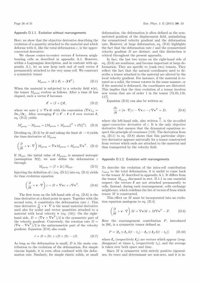
of 31 Eur. Phys. J. E (2015) 38: 33

Appendix D.1.1. Evolution without rearrangements

Here, we show that the objective derivative describing theevolution of a quantity attached to the material and whichdeforms with it, like the total deformation ε, is the upper-convected derivative.

We choose center-to-center vectors � between neigh-bouring cells as described in appendix A.1. However,within a Lagrangian description, and in contrast with ap-pendix A.1, let us now keep each end of each vector �permanently attached to the very same cell. We constructa symmetric tensor

Mperm = 〈� ⊗ �〉 = 〈� �T 〉. (D.1)

When the material is subjected to a velocity field v(r),the tensor Mperm evolves as follows. After a time dt haselapsed, such a vector � becomes

�′ = (I + ξ)�, (D.2)

where we note ξ ≡ ∇v dt with the convention (∇v)ij =∂vi/∂rj . After averaging �′ ⊗ �′ − � ⊗ � over vectors �,eq. (D.2) yields

M ′perm − Mperm = ξMperm + MpermξT + O(ξ2). (D.3)

Dividing eq. (D.3) by dt and taking the limit dt → 0 yieldsthe time-derivative of Mperm

(∂

∂t+ v · ∇

)Mperm = ∇vMperm + Mperm∇vT . (D.4)

If Minit, the initial value of Mperm, is assumed isotropic(assumption H2), we now define the deformation εthrough:

Mperm = (I + 2ε)Minit. (D.5)

Injecting the definition of ε (eq. (D.5)) into eq. (D.4) yieldsits time evolution equation

(∂

∂t+ v · ∇

)ε = D + ∇vε + ε∇vT . (D.6)

The first term on the left-hand side of eq. (D.6) is thetime derivative at a fixed point in space. Together with thesecond term, it constitutes the deformation rate ε. Thistime derivative ∂

∂t + v · ∇ is the usual material derivativeused also for scalar and vector quantities attached to amaterial with local velocity v (eq. (10)). On the right-hand side, D = (∇v + ∇vT )/2 is the symmetric part ofthe velocity gradient. Conversely, the rotation rate Ω =(∇v − ∇vT )/2 is the antisymmetric part of the velocitygradient. Equation (D.6) also reads

ε = D + Dε + εD + Ωε − εΩ. (D.7)

As long as the deformation is small, D is the main con-tribution to the evolution of the deformation. For simpleviscous liquids, it is even often confused with the defor-mation rate. Similarly, for simple elastic solids, at small

deformation, the deformation is often defined as the sym-metrised gradient of the displacement field, assimilatingthe symmetrised velocity gradient and the deformationrate. However, at large deformation, eq. (D.6) highlightsthe fact that the deformation rate ε and the symmetrisedvelocity gradient D are distinct, and this distinction iscritical throughout the present appendix.

In fact, the last two terms on the right-hand side ofeq. (D.6) are nonlinear, and become important at large de-formation. They are specific to (rank two) tensors. Theyreflect the fact that the natural coordinates used to de-scribe a tensor attached to the material are altered by thelocal velocity gradient. For instance, if the material is ro-tated as a solid, the tensor rotates in the same manner, orif the material is deformed, the coordinates are distorted.This implies that the time evolution of a tensor involvesnew terms that are of order 1 in the tensor [73,85,116,117].

Equation (D.6) can also be written as

∂ε

∂t+ (v · ∇) ε −∇v ε − ε∇vT = D, (D.8)

where the left-hand side, also written∇ε , is the so-called

upper-convective derivative of ε. It is the only objectivederivative that ensures that the dynamical equations re-spect the principle of covariance [118]. The derivation fromeq. (D.1) to eq. (D.8) shows that this particular objec-tive derivative appears univocally for a tensor constructedfrom vectors which ends are attached to the material andthus transported by the velocity field.

Appendix D.1.2. Evolution with rearrangements

To describe the evolution of the intra-cell contributionεintra to the total deformation, it is useful to come backto the tensor M described in appendix A.1. It differs fromthe tensor Mperm discussed in sect. D.1.1 in one essentialrespect: the vectors � are not attached permanently tocells. Instead, during each rearrangement, cells exchangeneighbours, which redefines the list of vectors � from whichtensor M is constructed.

This effect on M must be incorporated into an evolu-tion equation analogous to eq. (D.4)

(∂

∂t+ v · ∇

)M = ∇vM + M∇vT − P. (D.9)

Here the rearrangement contribution P , introducedin [68], is a symmetric tensor defined as

P = 〈�a ⊗ �a δ(t − ta) − �d ⊗ �d δ(t − td)〉 (D.10)

where �a (respectively �d) are vectors which appear (resp.disappear) at times ta (respectively td), and the averageis taken over both space and time.

Since M is symmetric with strictly positive eigenval-ues, its trace and determinant are non-zero, and it is in-

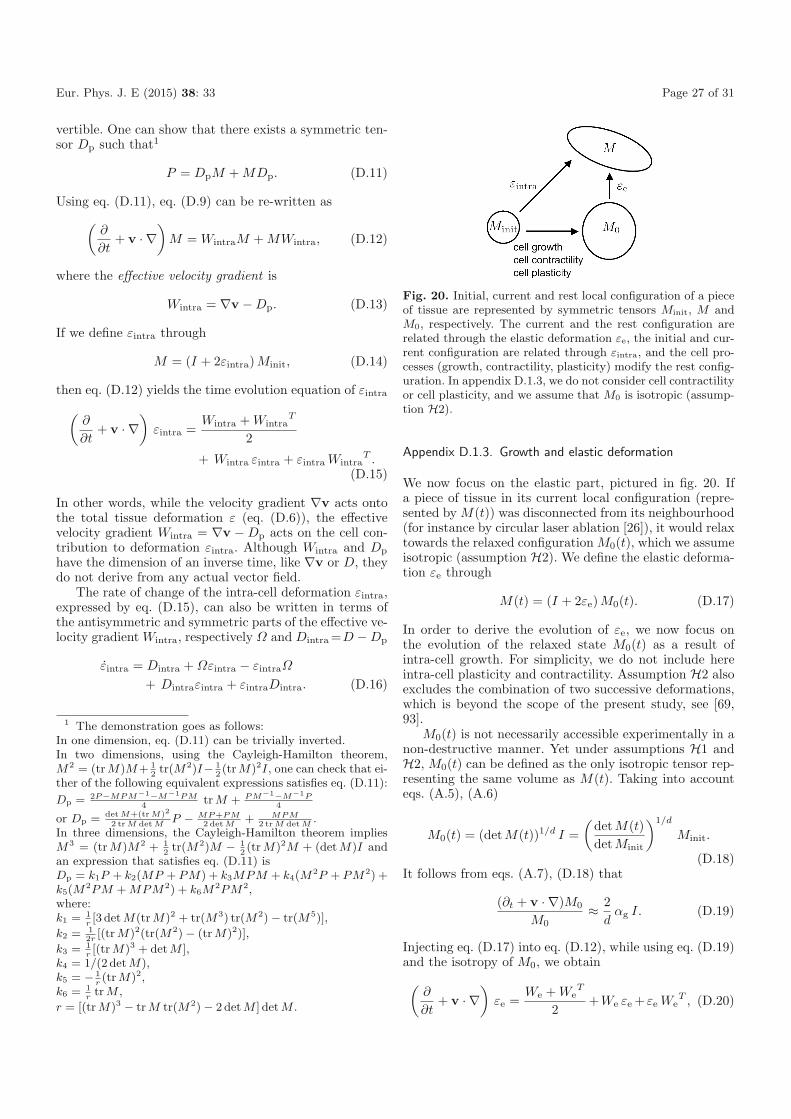
Eur. Phys. J. E (2015) 38: 33 of 31

vertible. One can show that there exists a symmetric ten-sor Dp such that1

P = DpM + MDp. (D.11)

Using eq. (D.11), eq. (D.9) can be re-written as(

∂

∂t+ v · ∇

)M = WintraM + MWintra, (D.12)

where the effective velocity gradient is

Wintra = ∇v − Dp. (D.13)

If we define εintra through

M = (I + 2εintra)Minit, (D.14)

then eq. (D.12) yields the time evolution equation of εintra

(∂

∂t+ v · ∇

)εintra =

Wintra + WintraT

2

+ Wintra εintra + εintra WintraT .

(D.15)

In other words, while the velocity gradient ∇v acts ontothe total tissue deformation ε (eq. (D.6)), the effectivevelocity gradient Wintra = ∇v − Dp acts on the cell con-tribution to deformation εintra. Although Wintra and Dp

have the dimension of an inverse time, like ∇v or D, theydo not derive from any actual vector field.

The rate of change of the intra-cell deformation εintra,expressed by eq. (D.15), can also be written in terms ofthe antisymmetric and symmetric parts of the effective ve-locity gradient Wintra, respectively Ω and Dintra =D − Dp

εintra = Dintra + Ωεintra − εintraΩ

+ Dintraεintra + εintraDintra. (D.16)

1 The demonstration goes as follows:In one dimension, eq. (D.11) can be trivially inverted.In two dimensions, using the Cayleigh-Hamilton theorem,M2 = (tr M)M+ 1

2tr(M2)I− 1

2(tr M)2I, one can check that ei-

ther of the following equivalent expressions satisfies eq. (D.11):

Dp = 2P−MPM−1−M−1PM4

tr M + PM−1−M−1P4

or Dp = det M+(tr M)2

2 tr M det MP − MP+PM

2 det M+ MPM

2 tr M det M.

In three dimensions, the Cayleigh-Hamilton theorem impliesM3 = (tr M)M2 + 1

2tr(M2)M − 1

2(tr M)2M + (det M)I and

an expression that satisfies eq. (D.11) isDp = k1P + k2(MP + PM) + k3MPM + k4(M

2P + PM2) +k5(M

2PM + MPM2) + k6M2PM2,

where:k1 = 1

r[3 det M(tr M)2 + tr(M3) tr(M2) − tr(M5)],

k2 = 12r

[(tr M)2(tr(M2) − (tr M)2)],

k3 = 1r[(tr M)3 + det M ],

k4 = 1/(2 det M),k5 = − 1

r(tr M)2,

k6 = 1r

tr M ,

r = [(tr M)3 − tr M tr(M2) − 2 det M ] det M .

Fig. 20. Initial, current and rest local configuration of a pieceof tissue are represented by symmetric tensors Minit, M andM0, respectively. The current and the rest configuration arerelated through the elastic deformation εe, the initial and cur-rent configuration are related through εintra, and the cell pro-cesses (growth, contractility, plasticity) modify the rest config-uration. In appendix D.1.3, we do not consider cell contractilityor cell plasticity, and we assume that M0 is isotropic (assump-tion H2).

Appendix D.1.3. Growth and elastic deformation

We now focus on the elastic part, pictured in fig. 20. Ifa piece of tissue in its current local configuration (repre-sented by M(t)) was disconnected from its neighbourhood(for instance by circular laser ablation [26]), it would relaxtowards the relaxed configuration M0(t), which we assumeisotropic (assumption H2). We define the elastic deforma-tion εe through

M(t) = (I + 2εe)M0(t). (D.17)

In order to derive the evolution of εe, we now focus onthe evolution of the relaxed state M0(t) as a result ofintra-cell growth. For simplicity, we do not include hereintra-cell plasticity and contractility. Assumption H2 alsoexcludes the combination of two successive deformations,which is beyond the scope of the present study, see [69,93].

M0(t) is not necessarily accessible experimentally in anon-destructive manner. Yet under assumptions H1 andH2, M0(t) can be defined as the only isotropic tensor rep-resenting the same volume as M(t). Taking into accounteqs. (A.5), (A.6)

M0(t) = (detM(t))1/d I =(

det M(t)det Minit

)1/d

Minit.

(D.18)It follows from eqs. (A.7), (D.18) that

(∂t + v · ∇)M0

M0≈ 2

dαg I. (D.19)

Injecting eq. (D.17) into eq. (D.12), while using eq. (D.19)and the isotropy of M0, we obtain(

∂

∂t+ v · ∇

)εe =

We + WeT

2+We εe + εe We

T , (D.20)

of 31 Eur. Phys. J. E (2015) 38: 33

where the effective velocity gradient is

We = ∇v − Dp − αgI

d. (D.21)

The effective velocity gradient We acts on the elastic de-formation, εe. Equation (D.20) has the same structure aseq. (D.15).

The rate of change of the elastic deformation, εe, ex-pressed by eq. (D.20), can also be written in terms of theantisymmetric and symmetric parts of the effective ve-locity gradient We, respectively Ω = (∇v − ∇vT )/2 andDe = D − Dp − αg I/d

εe = De + Ωεe − εeΩ + Deεe + εeDe. (D.22)

Appendix D.1.4. Evolution of the (large) deformation:summary

Equations (D.7), (D.16), (D.22) read

ε = (D + Dε + εD) + (Ωε − εΩ), (D.23)εk = (Dk + Dkεk + εkDk) + (Ωεk − εkΩ). (D.24)

Equations (D.23), (D.24) contain two parts delimitated byparentheses. First, a part due to an effective symmetrisedvelocity gradient Dk which depends on k (and which is thetrue symmetrised velocity gradient D only in eq. (D.23));second, another part due to the rotation rate Ω, whichdoes not depend on k.

If Qk is a non-mechanical tensor (sect. 3.4) constructedfrom a distribution of objects attached to element k ofthe rheological diagram, and if its rest value is isotropic,then its evolution is equal to its physical (intrinsic) rateof change Qintrinsic

k corrected by transport terms, like ineq. (D.24)

Qk = (Qintrinsick +DkQk+QkDk)+(ΩQk−QkΩ). (D.25)

Appendix D.2. Dissipation function formalism at largedeformation

The present appendix discusses how to implement largedeformations within the dissipation function formalism.Appendix D.2.1 provides a possible expression for theelastic energy that is suitable for large deformations. Ap-pendix D.2.2 derives the corresponding constitutive equa-tions. Appendices D.2.3 and D.2.4 detail the applicationto a simple example and to a complex one, respectively.

Appendix D.2.1. Elastic energy

At small deformations, the elastic response of an isotropicmaterial can be expressed in terms of only two scalar co-efficients, like in eq. (B.19). Conversely, at large elasticdeformations, eq. (B.19) is only one possibility to quan-tify the elastic energy. There is no fundamental reason

to exclude other isotropic, convex functions of the defor-mation, and other higher order terms would be possible.Since tr ε1 and dev ε1 do not represent any longer the purevolume and pure shape contributions of the deformationε1, eq. (B.19) is not technically convenient.

We now propose to define other quantities tr ε1 anddev ε1 which actually represent pure volume and shapecontributions of the deformation ε1 even at large defor-mations, as follows. They generalise tr ε1 and dev ε1 andcan be similarly defined for any εk.

As derived in appendix D.1.3, a quantity relevant todescribe large elastic deformation is the elongation I+2ε1,see eq. (D.17). The volume is proportional to the squareroot of its determinant det(I + 2ε1) (see appendix A.2).We suggest to decompose I + 2ε1 into the product of ascalar and a tensor of determinant unity

I + 2ε1 = [det(I + 2ε1)]1d

I + 2ε1

[det(I + 2ε1)]1d

. (D.26)

Since the decomposition is multiplicative, we take the log-arithm of eq. (D.26) to write an equation that tr ε1 anddev ε1 should obey

12

log(I + 2ε1) =tr ε1

dI + dev ε1 , (D.27)

or equivalently

ε1 =12

[exp

(2tr ε1

dI + 2dev ε1

)− I

]. (D.28)

For any symmetric, definite, positive tensor Q, there isan identity: log(detQ) = tr log Q. As a consequence, weobtain the definitions of tr ε1 and dev ε1

tr ε1 =12

tr [log(I + 2ε1)] , (D.29)

dev ε1 =12

dev [log(I + 2ε1)] . (D.30)

A natural possibility for the elastic energy, which tendstoward eq. (B.19) in the limit of small deformations, reads

E = G (dev ε1)2 +12K (tr ε1)2. (D.31)

The corresponding stress, which tends towards the elasticcontribution to eq. (B.14) in the limit of small deforma-tions, reads

σ = 2G dev ε1 + K tr ε1 I. (D.32)

Equation (D.31) is only an example of an isotropic, con-vex function of the deformation, and additional terms willgenerally be needed to describe the elasticity of any givenmaterial. The actual choice should be informed by rele-vant quantitative experimental measurements. In the in-compressible limit, eqs. (D.31), (D.32) become

tr ε1 = 0, (D.33)

E = G (dev ε1)2, (D.34)

dev σ = 2G dev ε1. (D.35)

Eur. Phys. J. E (2015) 38: 33 of 31

Appendix D.2.2. Constitutive equations

The dissipation function is written with the symmetrisedvelocity gradient D and its effective counterpart D1 (seeappendix D.1.4); since they always correspond to smalldeformation increments D dt and D1 dt, D is written usingthe usual traces and deviators, rather than with the largedeformation versions. Indeed, the reader may check, usingeqs. (D.7), (D.24), (D.29), (D.30) that

(∂t + v · ∇) [tr ε] = tr D, (D.36)

(∂t + v · ∇) [dev ε] = dev D, (D.37)

(∂t + v · ∇) [tr ε1] = trD1, (D.38)

(∂t + v · ∇) [dev ε1] = dev D1. (D.39)

The differentiation rule of the energy and dissipationfunction given by eqs. (B.10)-(B.13) is now rewritten usingD and D1

dev σ =∂D

∂ dev D+

∂E∂dev ε

, (D.40)

tr σ =∂D

∂ tr D+

∂E∂tr ε

, (D.41)

0 =∂D

∂ dev D1+

∂E∂dev ε1

, (D.42)

0 =∂D

∂ tr D1+

∂E∂tr ε1

. (D.43)

Appendix D.2.3. Simple example

The large deformations ingredients can be implemented inthe Maxwell viscoelastic liquid discussed in appendix B.2.

We rewrite the energy in terms of the large deforma-tion versions of the trace and deviator of the deforma-tions as in eq. (D.31), and the dissipation function as ineq. (B.20)

E = G (dev ε1)2 +12K (tr ε1)2, (D.44)

D = η (dev D − dev D1)2 +12χ (tr D − tr D1)2. (D.45)

From eqs. (D.40)-(D.43), we obtain the equivalent ofeqs. (B.15)-(B.18)

tr σ = χ d (tr D − tr D1), (D.46)dev σ = 2η (dev D − dev D1), (D.47)

0 = K d tr ε1 + χ d (tr D1 − tr D), (D.48)

0 = 2G dev ε1 + 2η (dev D1 − dev D). (D.49)

Equations (D.36)-(D.39) and (D.46)-(D.49) are suffi-cient to describe the material evolution using a closed setof equations. Once the set of equations is solved, the de-formations ε and ε1 are recovered from the volume andshape components using eq. (D.28).

The modulus of Dτ (called the “Weissenberg” num-ber) is dimensionless: it is the ratio of the relaxation timeto the typical time of the flow, and compares the materialviscoelastic properties with the kinetics. As long as thisnumber is moderately small, the situation remains simi-lar to the small deformation case: the nonlinear problem isstill well posed and efficient optimization algorithms couldbe used [91]. When this number becomes large, this prop-erty is lost in some cases, e.g. when the behavior of thematerial becomes close to an elastic body with large defor-mations in a complex geometry involving boundary layers.

Appendix D.2.4. Complex example

The energy and dissipation functions for tissue modellingrepresented by fig. 10 have been expressed explicitly insect. 3.5.2 in the limit of small elastic deformations. Atlarge elastic deformations, the corresponding expressionsbecome

E = G1 (dev (ε1))2 + G2 (dev (ε2))2, (D.50)D = ηcyto(dev Dintra − dev D1)2

+σY |dev D − dev Dintra − dev D3 − dev Dck|

+η3(dev D3)2 +12ηsw(tr Dintra − rsw + tr εck)2

+12ηapo(tr D − tr Dintra − tr Dck + rapo)2. (D.51)

The resulting dynamic equations (not shown) are comple-mented by the kinematic equations for the deformations

ε = D + Ωε − εΩ + Dε + εD, (D.52)ε1 = D1 + Ωε1 − ε1Ω + D1ε1 + ε1D1, (D.53)

εintra = Dintra + Ωεintra − εintraΩ

+Dintraεintra + εintraDintra. (D.54)

Equations (14), (22), (D.50)-(D.54) close the set of equa-tions which determine the evolution of the tissue.

References

1. E.F. Keller, Making sense of life: explaining biological de-velopment with models, metaphors, and machines (Har-vard University Press, 2002).

2. A. Huxley, R. Simmons, Nature 233, 533 (1971).3. Y. Fung, Biomechanics: Mechanical Properties of Living

Tissues (Springer Verlag, 2010).4. G. Forgacs, S.A. Newman, Biological Physics of the De-

veloping Embryo (Cambridge University Press, 2005).5. C.P. Heisenberg, Y. Bellaıche, Cell 153, 948 (2013).6. I.W. Hamley, Introduction to Soft Matter. Polymers, Col-

loids, Amphiphiles and Liquid Crustals (John Wiley andSons, 2010).

7. M. Caruel, J.M. Allain, L. Truskinovsky, Phys. Rev. Lett.110, 248108 (2013).

8. G. Forgacs, R.A. Foty, Y. Shafrir, M.S. Steinberg, Bio-phys. J. 74, 2227 (1998).

9. J. Ranft, M. Basan, J. Elgeti, J.F. Joanny, J. Prost, F.Julicher, Proc. Natl. Acad. Sci. U.S.A. 107, 20863 (2010).

of 31 Eur. Phys. J. E (2015) 38: 33

10. P. Marmottant, A. Mgharbel, J. Kafer, B. Audren, J.P.Rieu, J.C. Vial, B. van der Sanden, A.F.M. Maree, F.Graner, H. Delanoe-Ayari, Proc. Natl. Acad. Sci. U.S.A.106, 17271 (2009).

11. R. David, O. Luu, E.W. Damm, J.W.H. Wen, M. Nagel,R. Winklbauer, Development 141, 1 (2014).

12. F. Montel, M. Delarue, J. Elgeti, L. Malaquin, M. Basan,T. Risler, B. Cabane, D. Vignjevic, J. Prost, G. Cappelloet al., Phys. Rev. Lett. 107, 188102 (2011).

13. L. LeGoff, H. Rouault, T. Lecuit, Development 140, 4051(2013).

14. P. Fernandez, M. Maier, M. Lindauer, C. Kuffer, Z. Stor-chova, A. Bausch, PLoS One 6, e28965 (2011).

15. L. Wolpert, J. Smith, T. Jessell, P. Lawrence, E. Robert-son, E. Meyerowitz, Principles of Development (OxfordUniversity Press, 2006).

16. A. McMahon, W. Supatto, S.E. Fraser, A. Stathopoulos,Science 322, 1546 (2008).

17. P.J. Keller, A.D. Schmidt, J. Wittbrodt, E.H.K. Stelzer,Science 322, 1065 (2008).

18. N. Olivier, M.A. Luengo-Oroz, L. Duloquin, E. Faure, T.Savy, I. Veilleux, X. Solinas, D. Debarre, P. Bourgine, A.Santos et al., Science 329, 967 (2010).

19. J. Moosmann, A. Ershov, V. Altapova, T. Baumbach,M.S. Prasad, C. LaBonne, X. Xiao, J. Kashef, R. Hof-mann, Nature 497, 374 (2013).

20. U. Krzic, S. Gunther, T.E. Saunders, S.J. Streichan, L.Hufnagel, Nat. Methods 9, 730 (2012).

21. C. Bertet, L. Sulak, T. Lecuit, Nature 429, 667 (2004).22. B. Aigouy, R. Farhadifar, D.B. Staple, A. Sagner, J.C.

Roper, F. Julicher, S. Eaton, Cell 142, 773 (2010).23. F. Bosveld, I. Bonnet, B. Guirao, S. Tlili, Z. Wang, A.

Petitalot, R. Marchand, P.L. Bardet, P. Marcq, F. Graneret al., Science 336, 724 (2012).

24. O. Wartlick, A. Kicheva, M. Gonzalez-Gaitan, ColdSpring Harbor Persp. Biol. 1, a001255 (2009).

25. M.S. Hutson, Y. Tokutake, M.S. Chang, J.W. Bloor, S.Venakides, D.P. Kiehart, G.S. Edwards, Science 300, 145(2003).

26. I. Bonnet, P. Marcq, F. Bosveld, L. Fetler, Y. Bellaıche,F. Graner, J. R. Soc. Interface 9, 2614 (2012).

27. G.W. Brodland, V. Conte, P.G. Cranston, J. Veldhuis,S. Narasimhan, M.S. Hutson, A. Jacinto, F. Ulrich, B.Baum, M. Miodownik, Proc. Natl. Acad. Sci. U.S.A. 107,22111 (2010).

28. K.K. Chiou, L. Hufnagel, B.I. Shraiman, PLoS Comput.Biol. 8, e1002512 (2012).

29. S. Ishihara, K. Sugimura, J. theor. Biol. 313, 201 (2012).30. K. Sugimura, S. Ishihara, Development 140, 4091 (2013).31. J.L. Maıtre, H. Berthoumieux, S.F.G. Krens, G. Sal-

breux, F. Julicher, E. Paluch, C.P. Heisenberg, Science338, 253 (2012).

32. O. Campas, T. Mammoto, S. Hasso, R.A. Sperling, D.O’Connell, A.G. Bischof, R. Maas, D.A. Weitz, L. Ma-hadevan, D.E. Ingber, Nat. Methods 11, 183 (2014).

33. N. Borghi, M. Sorokina, O.G. Shcherbakova, W.I. Weis,B.L. Pruitt, W.J. Nelson, A.R. Dunn, Proc. Natl. Acad.Sci. U.S.A. 109, 12568 (2009).

34. X. Trepat, M.R. Wasserman, T.E. Angelini, E. Millet,D.A. Weitz, J.P. Butler, J.J. Fredberg, Nat. Phys. 5, 426(2009).

35. T.E. Angelini, E. Hannezo, X. Trepat, J.J. Fredberg, D.A.Weitz, Phys. Rev. Lett. 104, 168104 (2010).

36. A. Saez, E. Anon, M. Ghibaudo, O. du Roure, J.-M. diMeglio, P. Hersen, P. Silberzan, A. Buguin, B. Ladoux,J. Phys.: Condens. Matter 22, 194119 (2010).

37. M. Reffay, L. Petitjean, S. Coscoy, E. Grasland-Mongrain,F. Amblard, A. Buguin, P. Silberzan, Biophys. J. 100,2566 (2011).

38. X. Serra-Picamal, V. Conte, R. Vincent, E. Anon, D.T.Tambe, E. Bazellieres, J.P. Butler, J.J. Fredberg, X.Trepat, Nat. Phys. 8, 628 (2012).

39. A.R. Harris, L. Peter, J. Bellis, B. Baum, A.J. Kabla,G.T. Charras, Proc. Natl. Acad. Sci. U.S.A. 109, 16449(2012).

40. K. Doxzen, S.R.K. Vedula, M.C. Leong, H. Hirata, N.S.Gov, A.J. Kabla, B. Ladoux, C.T. Lim, Integr. Biol. 5,1026 (2013).

41. O. Cochet-Escartin, J. Ranft, P. Silberzan, P. Marcq, Bio-phys. J. 106, 65 (2014).

42. D. Gonzalez-Rodriguez, K. Guevorkian, S. Douezan, F.Brochard-Wyart, Science 338, 910 (2012).

43. K. Alessandri, B.R. Sarangi, V.V. Gurchenkov, B. Sinha,T.R. Kieling, L. Fetler, F. Rico, S. Scheuring, C. Lamaze,A. Simon et al., Proc. Natl. Acad. Sci. U.S.A. 110, 14843(2013).

44. A. Mgharbel, H. Delanoe-Ayari, J.P. Rieu, HFSP J. 3,213 (2009).

45. T.V. Stirbat, S. Tlili, T. Houver, C. Barentin, J.P. Rieu,H. Delanoe-Ayari, Eur. Phys. J. E 36, 84 (2013).

46. R. Tomer, K. Khairy, F. Amat, P.J. Keller, Nat. Methods9, 755 (2012).

47. T. Nagai, H. Honda, Philos. Mag. B 81, 699 (2001).48. A.F.M. Maree, V.A. Grieneisen, P. Hogeweg, The Cel-

lular Potts Model and biophysical properties of cells, tis-sues and morphogenesis, in Single Cell-Based Models inBiology and Medicine, edited by A.R.A. Anderson, M.Chaplain, K.A. Rejniak (Birkhauser Verlag, Basel, 2007)pp. 107–136.

49. D. Drasdo, S. Hoehme, M. Block, J. Stat. Phys. 128, 287(2007).

50. J. Solon, A. Kaya-Copur, J. Colombelli, D. Brunner, Cell137, 1331 (2009).

51. B. Vasiev, A. Balter, M. Chaplain, J.A. Glazier, C.J. Wei-jer, PLoS One 5, e10571 (2010).

52. G.W. Brodland, X. Chen, P. Lee, M. Marsden, HFSP J.4, 142 (2010).

53. A.J. Kabla, J. R. Soc. Interface 9, 3268 (2012).54. M.A. Wyczalkowski, Z. Chen, B.A. Filas, V.D. Varner,

L.A. Taber, Birth Defects Res. C 96, 132 (2012).55. M. Basan, J. Elgeti, E. Hannezo, W.J. Rappel, H. Levine,

Proc. Natl. Acad. Sci. U.S.A. 110, 2452 (2013).56. N. Sepulveda, L. Petitjean, O. Cochet, E. Grasland-

Mongrain, P. Silberzan, V. Hakim, PLoS Comput. Biol.9, e1002944 (2013).

57. Y. Li, H. Naveed, S. Kachalo, L.X. Xu, J. Liang, PLoSOne 9, e86725 (2014).

58. J. Ortega, Plant Physiol. 79, 318 (1985).59. D.P. Pioletti, L.R. Rakotomanana, Eur. J. Mech. A 19,

749 (2000).60. P. Nardinocchi, L. Teresi, J. Elast. 88, 27 (2007).61. M. Basan, T. Risler, J.F. Joanny, X. Sastre-Garau, J.

Prost, HFSP J. 3, 265 (2009).62. M. Basan, J.F. Joanny, J. Prost, T. Risler, Phys. Rev.

Lett. 106, 158101 (2011).63. K. Guevorkian, M.J. Colbert, M. Durth, S. Dufour, F.

Brochard-Wyart, Phys. Rev. Lett. 104, 218101 (2010).

Eur. Phys. J. E (2015) 38: 33 of 31

64. L. Preziosi, D. Ambrosi, C. Verdier, J. theor. Biol. 262,35 (2010).

65. P. Lee, C.W. Wolgemuth, PLoS Comput. Biol. 7,e1002007 (2011).

66. M.H. Kopf, L.M. Pismen, Soft Matter 9, 3727 (2012).67. E.E. Kuchen, S. Fox, P. Barbier de Reuille, R. Kennaway,

S. Bensmihen, J. Avondo, G.M. Calder, P. Southam, S.Robinson, A. Bangham et al., Science 335, 1092 (2012).

68. F. Graner, B. Dollet, C. Raufaste, P. Marmottant, Eur.Phys. J. E 25, 349 (2008).

69. S. Benito, C.-H. Bruneau, T. Colin, C. Gay, F. Molino,Eur. Phys. J. E 25, 225 (2008).

70. S. Benito, F. Molino, C.-H. Bruneau, T. Colin, C. Gay,Eur. Phys. J. E 35, 1 (2012).

71. I. Cheddadi, P. Saramito, B. Dollet, C. Raufaste, F.Graner, Eur. Phys. J. E 34, 1 (2011).

72. I. Cantat, S. Cohen-Addad, F. Elias, F. Graner, R.Hohler, O. Pitois, F. Rouyer, A. Saint-Jalmes, Foams:structure and dynamics, edited by S.J. Cox (Oxford Uni-versity Press, 2013).

73. J.G. Oldroyd, Proc. Roy. Soc. London A 200, 523 (1950).74. P. Chaikin, T. Lubensky, Principles of condensed matter

physics (Cambridge University Press, 1995).75. P.C. Martin, O. Parodi, P.S. Pershan, Phys. Rev. A 6,

2401 (1972).76. P.G. de Gennes, J. Prost, The Physics of Liquid Crystals,

2nd ed. (Oxford University Press, 1993).77. J. Toner, Y. Tu, S. Ramaswamy, Ann. Phys. 318, 170

(2005).78. E. Bertin, M. Droz, G. Gregoire, J. Phys. A 42, 445001

(2009).79. F. Julicher, K. Kruse, J. Prost, J.F. Joanny, Phys. Rep.

449, 3 (2007).80. M.C. Marchetti, J.F. Joanny, S. Ramaswamy, T.B. Liv-

erpool, J. Prost, M. Rao, R.A. Simha, Rev. Mod. Phys.85, 1143 (2013).

81. S.R. de Groot, P. Mazur, Non-Equilibrium Thermody-namics (Dover Publications, 1985).

82. L. Landau, E. Lifchitz, Statistical Physics (Butterworth-Heinemann, 1975).

83. B. Halphen, Q. Nguyen, J. Mec. 14, 39 (1975).84. G. Maugin, The thermomechanics of plasticity and frac-

ture (Cambridge, 1992).85. P. Saramito, Methodes numeriques en fluides complexes:

theorie et algorithmes (CNRS-CCSD, 2012), http://

cel.archives-ouvertes.fr/cel-00673816.86. G.T. Houlsby, Dissipation rate functions, Pseudopoten-

tials, Potentials and Yield Surfaces, in Beyond the SecondLaw (Springer-Verlag, 2014) pp. 73–95.

87. P. Saramito, J. Non-Newt. Fluid Mech. 145, 1 (2007).88. P. Saramito, J. Non-Newt. Fluid Mech. 158, 154 (2009).89. P.L. Tallec, Numerical analysis of viscoelastic problems

(Masson, 1990).90. I. Cheddadi, P. Saramito, F. Graner, J. Rheol. 56, 213

(2012).91. I. Cheddadi, P. Saramito, J. Non-Newtonian Fluid Mech.

202, 13 (2013).92. L.A. Taber, Nonlinear Theory of Elasticity: Applications

in Biomechanics (World Scientific, 2004).93. S. Benito, Ph.D. thesis, Universite Bordeaux 1, Bordeaux,

France (2009), http://tel.archives-ouvertes.fr/

tel-00525106/fr/.94. I. Cheddadi, Ph.D. thesis, Universite Joseph-Fourier

- Grenoble I, Grenoble, France (2010), http://tel.

archives-ouvertes.fr/tel-00497436/.

95. E.M. Schoetz, M. Lanio, J.A. Talbot, M.L. Manning, J.R. Soc. Interface 10, 20130726 (2013).

96. K.D. Nnetu, M. Knorr, J. Kas, M. Zink, New J. Phys.14, 115012 (2013).

97. D. Bi, J.H. Lopez, J.M. Schwarz, M.L. Manning, SoftMatter 10, 1885 (2014).

98. N. Roquet, P. Saramito, Comput. Appl. Meth. Mech. En-grg. 192, 3317 (2003).

99. A. Puliafito, L. Hufnagel, P. Neveu, S. Streichan, A. Si-gal, D.K. Fygenson, B.I. Shraiman, Proc. Natl. Acad. Sci.U.S.A. 109, 739 (2012).

100. T. Bittig, O. Wartlick, A. Kicheva, M. Gonzalez-Gaitan,F. Julicher, New J. Phys. 11, 063001 (2008).

101. T. Bittig, O. Wartlick, M. Gonzalez-Gaitan, F. Julicher,Eur. Phys. J. E 30, 93 (2009).

102. T. McMahon, Muscles, Reflexes, and Locomotion(Princeton University Press, Princeton, 1984).

103. K. Kruse, J.F. Joanny, F. Julicher, J. Prost, K. Sekimoto,Phys. Rev. Lett. 92, 078101 (2004).

104. J. Etienne, J. Fouchard, D. Mitrossilis, N. Bufi, P.Durand-Smet, A. Asnacios, Proc. Natl. Acad. Sci. U.S.A.112, 2740 (2015).

105. A.M. Sonnet, E.G. Virga, Phys. Rev. E 64, 031705(2001).

106. A.M. Sonnet, P.L. Maffettone, E.G. Virga, J. Non-Newtonian Fluid Mech. 119, 51 (2004).

107. A. Desmaison, C. Frongia, K. Grenier, B. Ducommun, V.Lobjois, PLoS One 8, e80447 (2013).

108. P. Preira, M.P. Valignat, J. Bico, O. Theodoly, Biomi-crofluidics 7, 024111 (2013).

109. T.V. Stirbat, A. Mgharbel, S. Bodennec, K. Ferri, H.C.Mertani, J.P. Rieu, H. Delanoe-Ayari, PLoS One 8,e52554 (2013).

110. C. Blanch-Mercader, J. Casademunt, J.F. Joanny, Eur.Phys. J. E 37, 41 (2014).

111. G.B. Blanchard, A.J. Kabla, N.L. Schultz, L.C. Butler, B.Sanson, N. Gorfinkiel, L. Mahadevan, R.J. Adams, Nat.Methods 6, 458 (2009).

112. L.C. Butler, G.B. Blanchard, A.J. Kabla, N.J. Lawrence,D.P. Welchman, L. Mahadevan, R.J. Adams, B. Sanson,Nat. Cell Biol. 11, 859 (2006).

113. J.S. Bois, F. Julicher, S.W. Grill, Phys. Rev. Lett. 106,028103 (2011).

114. P. Marcq, Eur. Phys. J. E 37, 29 (2014).115. G. Duclos, S. Garcia, H.G. Yevick, P. Silberzan, Soft Mat-

ter 10, 2346 (2014).116. D.D. Joseph, Fluid dynamics of viscoelastic liquids

(Springer, 1990).117. P. Oswald, Rheophysics: The Deformation and Flow of

Matter (Cambridge University Press, 2009).118. E. Rouhaud, B. Panicaud, R. Kerner, Comput. Mater.

Sci. 77, 120 (2013).

The authors represent a collaboration from different fieldsthat complement each other for the topic of the present arti-cle: biology, biophysics, theoretical physics and applied math-ematics. Some of the authors are members of the Academy ofBradylogists. They declare that scientific work takes time. Ittakes time to think differently and sometimes it takes time tobe wrong. They believe that collaboration is more fecund thancompetition, and that only time can state about the quality ofa research work, as opposed to the excessive use of labels, fastevaluations and judgments.

colloquium: mechanical formalisms for tissue dynamics · colloquium: mechanical formalisms for...

Documents