columbia river gorge visibility and air · pdf filecolumbia river gorge visibility and air...

COLUMBIA RIVER GORGE VISIBILITY AND AIRQUALITY STUDY

Working Draft: Existing Knowledge and AdditionalRecommended Scientific Assessment to Consider

June 7, 2001(updated 7/26/01)

Prepared by:

Mark C. Green, Ph.D. Division of Atmospheric Sciences

Desert Research InstituteLas Vegas, NV

With Assistance from:

Marc L. Pitchford, Ph.D.Special Operations & Research Division

Air Resources LaboratoryNational Oceanic and Atmospheric Administration

Las Vegas, NV

Ralph E. Morris Principal

Environ International Corp.Novato, Calif

Kent Norville Ph.D.Atmospheric Scientist

Air SciencesPortland, Or

And assistance from and consultation with:The Columbia River Gorge NSA Air Quality Project Technical Team

2

TABLE OF CONTENTS

1 INTRODUCTION ........................................................................................................ 41.1 What air quality issues will this study address? ..................................................... 41.2 Goals and Objectives .............................................................................................. 51.3 Guide to study plan ................................................................................................. 6

2 SUMMARY OF EXISTING KNOWLEDGE.............................................................. 82.1 Emissions ................................................................................................................ 82.2 Meteorology and Climatography: ......................................................................... 162.3 Visibility and Air Quality ..................................................................................... 18

3 HYPOTHESES TO BE TESTED............................................................................... 334 ELEMENTS OF THE PROPOSED STUDY............................................................. 50

4.1 MONITORING COMPONENT........................................................................... 504.1.1 Optical measurements................................................................................... 504.1.2 Aerosol and Gaseous Measurements ............................................................ 534.1.3 Meteorological measurements ...................................................................... 554.1.4 Tracers........................................................................................................... 56

4.1.5. Data Analysis/Conceptual Model Development............................................. 614.2 EMISSIONS COMPONENT................................................................................ 644.3 MODELING COMPONENT ............................................................................... 664.3.1 Emissions Modeling ..................................................................................... 674.3.2 Air Quality Modeling.................................................................................... 69

5 PROPOSED STUDY STRUCTURE ......................................................................... 745.1 Phased Approach Concept .................................................................................... 745.2 Rationale for elements of the Technical Foundation study .................................. 755.3 Development of Phase 2 ....................................................................................... 77

6 DATA MANAGEMENT............................................................................................ 787 QUALITY ASSURANCE.......................................................................................... 818 SUGGESTIONS ON STUDY MANAGEMENT STRUCTURE.............................. 839 BUDGET .................................................................................................................... 8410 REFERENCES: ........................................................................................................ 8611 LIST OF ACRONYMS ............................................................................................ 88

3

Columbia River Gorge NSA Air Quality Project Technical Team Members

Allen, Philip – Oregon Dept. of Environmental QualityAllen, Tim – Washington State Dept. of Ecology

Bachman, Robert – USDA, Forest Service, Region 6Bowman, Clint – Washington State Dept. of Ecology

Figueroa-Kaminsky, Cristiana – Washington State Dept. of EcologyIslam, Mahbubul – U.S. Environmental Protection Agency, Region 10

Krietzer, Natalia – Southwest Clean Air AgencyLazarev, Svetlana – Oregon Dept. of Environmental Quality

Mairose, Paul (alternate) – Southwest Clean Air AgencyMorris, Ralph – Environ International Corporation

Norville, Kent – Air Sciences Incorporated Otterson, Sally – Washington State Dept. of Ecology

Pitchford, Marc – National Oceanic and Atmospheric AdministrationRose, Keith – U.S. Environmental Protection agency, Region 10

Schaaf, Mark – Air Sciences IncorporatedStocum, Jeffrey – Oregon Dept. of Environmental Quality

Van Haren, Frank – Washington State Dept. of Ecology (Technical Team Chair)Vimont, John – USDI, National Park Service

Advisor to the team:Green, Mark – Desert Research Institute

4

1 INTRODUCTION

This scientific assessment study plan for a Columbia River Gorge air quality andvisibility study was prepared to assist in the development of an overall work plan for theColumbia River Gorge Air Quality Project. This project includes a series of steps fromscientific investigation through development of a comprehensive regional air qualitystrategy to implementation of that strategy. This study plan focuses on the scientificinvestigation component of the overall work plan. It stands as the technical foundation forwork to come. It is dynamic in that specific tasks and costs associated with them willchange as monitoring, emission inventory, and modeling methods are adapted based oninformation gathered over the length of this process – in essence this document should betreated as a working draft that evolves over the period of this assessment.

In May 2000 the Commission adopted an amendment to the Gorge Management Plan thatcalls for the protection and enhancement of Gorge air quality. The amendment directedthe states of Oregon and Washington, working with the U.S. Forest Service and theSouthwest Clean Air Agency and in consultation with affected stakeholders to develop awork plan. The purpose of the work plan, among other things, is to establish timelines forthe gathering and analysis of necessary Gorge air quality data and, ultimately, for thedevelopment and implementation of an air quality protection strategy.

A peer-review workshop was held March 14-15, 2001 in Cascade Locks, Oregon tosolicit comments from experts on a “strawman” scientific assessment study plan. Over50 national and international air quality scientists attended. This plan has incorporatedmany helpful suggestions from the reviewers.

The role of scientific assessment as outlined in this study plan is not intended to addressthe two overall purposes of the Scenic Area Act. The two purposes are: 1) protect andenhance scenic, cultural, recreational and natural resources and, 2) protect and supportthe economy of existing urban areas in the Scenic Area (consistent with the firstpurpose). Balancing these two purposes is the role of decision-makers (with input fromthe public and stakeholders), not scientists. How this balance will be assessed isaddressed in other parts of the overall work plan (for instance, a plan for economicanalysis of strategy alternatives is included elsewhere in the work plan). The scientificinvestigation only provides a technical foundation by characterizing air quality,identifying sources that contribute to air quality problems, and by providing tools toassess changes in air quality based on changes in emissions. The goals and objectives arediscussed below.

1.1 What air quality issues will this study address?This study will focus its scope on pollutants that affect visibility and pollutants that leadto the formation of ozone and acid deposition. The pollutants that affect visibility are: sulfate (converted from sulfur dioxide) nitrate (converted from nitrogen dioxide) organic carbon (including volatile organic carbon species) elemental carbon

5

soil dust. Because such a small amount of these pollutants can cause significant visibilityimpairment, reducing these pollutants sufficient to protect visibility will result insignificant benefits to many other air quality issues of concern. The pollutants that leadto the formation of ozone (nitrogen oxides and VOC’s) and acid deposition (sulfur andnitrogen oxides) are contained in this list of visibility impairing pollutants. Thereforethere is a direct link between improving visibility and reducing ozone and aciddeposition.

This study will not address air borne toxic pollution. Toxic air pollutants are beingaddressed through each states air toxic programs that are already in place.

1.2 Goals and Objectives

This study plan will be incorporated as an appendix to the overall work plan discussedabove and is intended to describe a study that would lead to a general understanding ofthe sources of aerosols and visibility, and other air quality components such as effects oncultural resources, agricultural health, ecosystem disturbance, and ozone effects onvegetation and humans. It includes identification of model development and evaluationneeded for assessment of future emission scenarios to be developed under the overallwork plan. It also acknowledges that long-term monitoring needs to be done to evaluatetrends and effects of emissions scenarios to be implemented under the overall work plan.

The goals of the study are to characterize current air quality, visibility andmeteorological conditions in the Scenic Area, identify sources affecting air qualityand visibility in the Scenic Area, and to develop and evaluate models to be used toassess changes in air quality and visibility within the Scenic Area due to changes inemissions. In order to determine the important physical processes that must be capturedby models, a substantial monitoring component for the study is proposed. Themonitoring component of the study will:

• lead to the understanding of the physical processes at work, i.e. the developmentof conceptual models, a major objective of the study

• help identify sources, source categories and source regions that affect air qualityand visibility in the Scenic Area

• provide direct input to mathematical models by data, including1) wind data from radar wind profilers and radiosondes2) boundary conditions for aerosols and gases

• provide data for model evaluation.

In a simple situation such as flat terrain, an isolated point source, and clear skies, modelapplication and monitoring programs would be relatively straightforward. However, inthe Scenic Area, there is highly complex terrain and substantial moisture, including fogand low clouds. There are also significant uncertainties in emissions inventories. Thus, arobust monitoring program is proposed that will help determine what the important

6

processes are that the models must simulate, provide information for model input andevaluation, and to help in the evaluation and further development of the emissionsestimates for sources of important chemical compounds. For example, if cloud-waterchemistry processes are very important, then models that have sophisticated cloud-chemistry mechanisms would be needed.

Some modeling will be helpful in developing the conceptual models, such asconfirmation of general flow directions that can be used to evaluate the reasonableness ofreceptor models, for example. Selection of modeling tools that will be recommendedfor assessment of changes in future air quality with various emissions scenarios willbe finalized after the conceptual models have been developed.

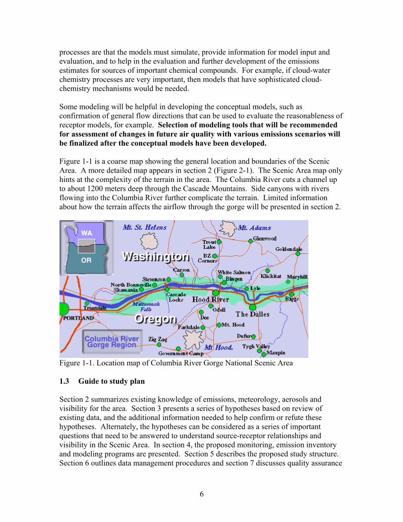
Figure 1-1 is a coarse map showing the general location and boundaries of the ScenicArea. A more detailed map appears in section 2 (Figure 2-1). The Scenic Area map onlyhints at the complexity of the terrain in the area. The Columbia River cuts a channel upto about 1200 meters deep through the Cascade Mountains. Side canyons with riversflowing into the Columbia River further complicate the terrain. Limited informationabout how the terrain affects the airflow through the gorge will be presented in section 2.

Figure 1-1. Location map of Columbia River Gorge National Scenic Area

1.3 Guide to study plan

Section 2 summarizes existing knowledge of emissions, meteorology, aerosols andvisibility for the area. Section 3 presents a series of hypotheses based on review ofexisting data, and the additional information needed to help confirm or refute thesehypotheses. Alternately, the hypotheses can be considered as a series of importantquestions that need to be answered to understand source-receptor relationships andvisibility in the Scenic Area. In section 4, the proposed monitoring, emission inventoryand modeling programs are presented. Section 5 describes the proposed study structure.Section 6 outlines data management procedures and section 7 discusses quality assurance

7

needs. Section 8 recommends a program management structure. Budget estimates aregiven in Section 9. References are presented in Section 10.

8

2 SUMMARY OF EXISTING KNOWLEDGE.

This section presents an overview of background information regarding, emissions,meteorology, air quality, and visibility in the Scenic Area. Additional information iscontained in the documents: “Some Characteristics of Aerosols and Haze, AerosolTransport and Emissions Sources Affecting the Columbia River Gorge NSA” preparedby the Washington State Department of Ecology and the Oregon Department ofEnvironmental Quality (2001) and “On the Composition and Patterns of Aerosols andHaze Within the Columbia River Gorge: September 1, 1996- September 30, 1998” byCore (2001).

2.1 Emissions

Figure 2-1 is a location map showing the Scenic Area, nearby Class I areas and majorcities, highways, railroads, and point sources.

Note that the Portland, Oregon/ Vancouver, Washington urban area (population about 1.8million) is located immediately to the west of the Scenic Area. The Centralia powerplant, with 1996 emissions of 78,000 tons of SO2, or 47% of the point source SO2emissions in EPA Region 10 (Oregon, Washington, Idaho, Alaska) (USEPA, 2001) islocated at the north edge of the map, just above Chehalis, about 135 km from the ScenicArea. The Centralia powerplant is scheduled to have 90% controls on one unit byDecember 2001, and 90% control on the other unit by December 2002. The Boardman

Ñ

Ñ ÑÑÑ

Ñ

ÑÑ

ÑÑ

Ñ

ÑÑ

Ñ

Ñ

Ñ

ÑÑ Ñ

Ñ

ÑÑ Ñ

Ñ

Ñ

ÑÑ

Ñ

Ñ

Ñ

ÑÑ

Ñ

Ñ

Ñ

Ñ

Ñ

Ñ

Ñ

Ñ

Ñ

ÑÑ

Ñ

Ñ

Ñ

Ñ

Ñ

Ñ

Ñ

Ñ

Ñ

Ñ

ÑÑÑ

Ñ

ÑÑ

Ñ

Ñ

Ñ

Ñ

ÑÑ

ÑÑ

Ñ

Ñ

Ñ

Ñ

Ñ

Ñ ÑÑÑÑ

ÑÑÑ

Ñ

ÑÑ

Ñ

Ñ

Ñ

ÑÑ

Ñ

Ñ

ÑÑÑ

Ñ

Ñ

Ñ

Ñ

Ñ

Ñ

Ñ

Ñ

Ñ

Ñ

Ñ

Ñ

Ñ

Ñ

Ñ

Ñ

Ñ

Ñ

Ñ

ÑÑ

Ñ

ÑÑ

ÑÑ Ñ

Ñ

Ñ

Ñ

Ñ

Ñ

Ñ

Ñ

Ñ

Ñ

Ñ

ÑÑ

ÑÑ

Ñ

ÑÑÑÑÑ

ÑÑ

Ñ

Ñ

ÑÑ

Ñ

Ñ ÑÑ

ÑÑ

Ñ Ñ

Ñ

Ñ

Ñ

Ñ

ÑÑÑ

ÑÑ

Ñ

Ñ Ñ ÑÑ

Ñ

Ñ

Ñ

Ñ

Ñ

ÑÑ

Ñ

ÑÑ

Ñ

ÑÑ

Ñ

ÑÑÑ ÑÑÑ Ñ

Ñ

ÑÑ

Ñ

Ñ

Ñ

ÑÑ

ÑÑ

Ñ

ÑÑ

Ñ

Ñ

Ñ

Ñ

ÑÑÑ

Ñ

Ñ

ÑÑÑ

Ñ

Ñ

Ñ

Ñ

Ñ

ÑÑ

ÑÑ

Ñ

Ñ

Ñ

Ñ

ÑÑÑ

Ñ

ÑÑ

Ñ

Ñ

Ñ

Ñ

Ñ

Ñ Ñ

Ñ

Ñ

Ñ

Ñ

Ñ

Ñ

Ñ

Ñ

Ñ

Ñ

Ñ

Ñ

Ñ

Ñ

Ñ

Ñ

Ñ

Ñ

Ñ

ÑÑÑÑ

Ñ

ÑÑ

ÑÑ

ÑÑ

ÑÑ

Ñ

Ñ

Ñ

ÑÑ

Ñ

Ñ

ÑÑÑ

ÑÑ

ÑÑÑÑ

Ñ

Ñ

Ñ

ÑÑÑÑ

Ñ

Ñ

ÑÑÑ

Ñ

Ñ

#Y

#Y

Vancouver

Yakima

Kelso

Longview

Chehalis

Sunnyside

mond

Prosser

Kalama

Goldendale

North Bonnevil le

StevensonBingen

Cathlamet

Portland

Salem

Albany

Hillsboro

Corvall is

Beaverton

The Dalles

Oregon City

Madras

Arlington

Hood River

Cascade Locks

Mosier

D

Mt. AdamsWilderness

Mt. HoodWilderness

Columbia River Gorge National Scenic Area

Camas

White Salmon

Wishram

Mt. ZionTroutdale

LI NN

ATSOP

Goat RocksWilderness

Saint Helens

Mt. JeffersonWilderness

McMinnville

N

EW

SCountyScenic Area

CityRailroads

RoadsÑ Point Source

Class I Area#Y IMPROVE Site

9

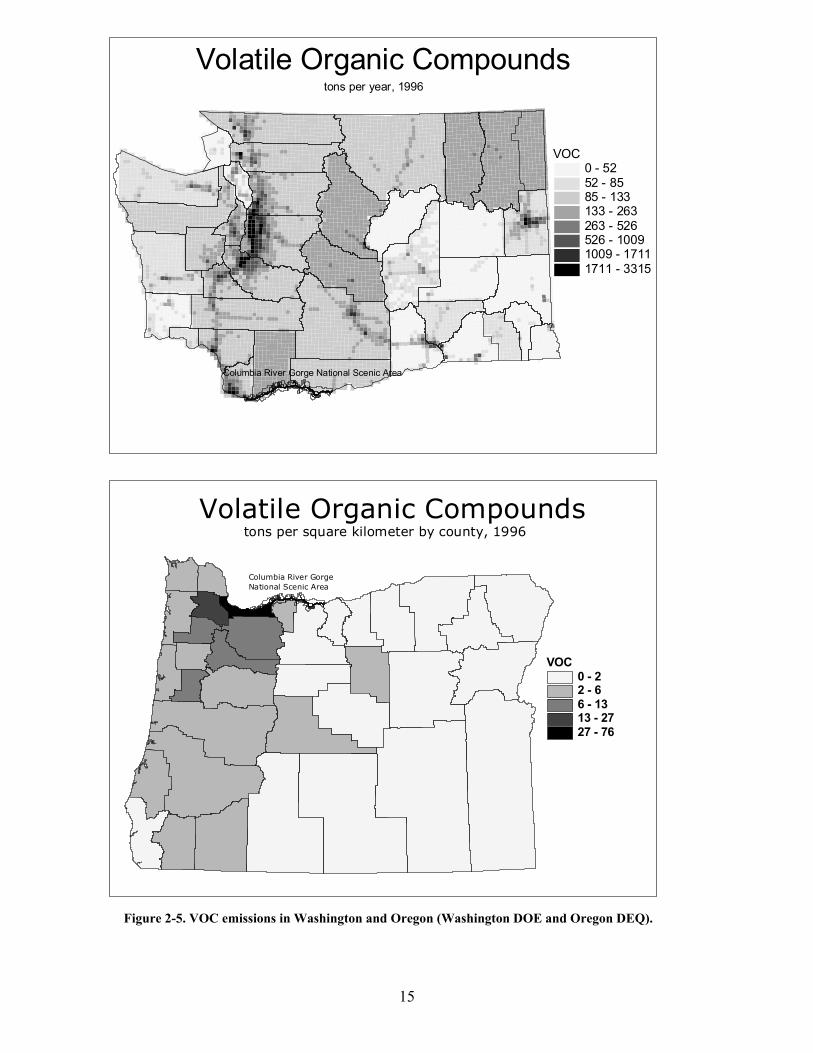
powerplant, located about 100 km east of the Scenic Area had SO2 emissions of 16,578tons and NOX emissions of 8949 tons in 1999 (Oregon Department of EnvironmentalQuality). Sources within the Scenic Area include aluminum smelters, cities of TheDalles, and Hood River, highways, ships, and 2 railroads. Up the Columbia River fromthe Scenic Area are the Tri-cities (Richland-Pasco-Kennewick), Yakima, and Spokane (ofpotential interest mainly in winter). Also to be considered, particularly in summer, areemissions from the Willamette Valley, Longview, the Seattle metropolitan area, andpossibly sources to Vancouver, British Columbia. Emissions maps prepared by theWashington Department of Ecology and Oregon Department of Environmental Qualityare shown in Figures 2.2-2.5. The Washington emissions are allocated to grid cells 5 kmon a side. The Oregon emissions inventories are currently at the county level.

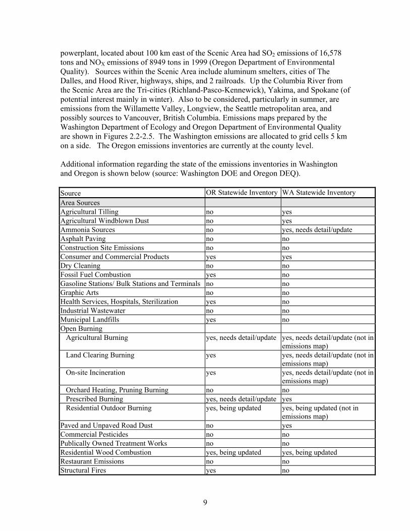
Additional information regarding the state of the emissions inventories in Washingtonand Oregon is shown below (source: Washington DOE and Oregon DEQ).

Source OR Statewide Inventory WA Statewide InventoryArea SourcesAgricultural Tilling no yesAgricultural Windblown Dust no yesAmmonia Sources no yes, needs detail/updateAsphalt Paving no noConstruction Site Emissions no noConsumer and Commercial Products yes yesDry Cleaning no noFossil Fuel Combustion yes noGasoline Stations/ Bulk Stations and Terminals no noGraphic Arts no noHealth Services, Hospitals, Sterilization yes noIndustrial Wastewater no noMunicipal Landfills yes noOpen Burning Agricultural Burning yes, needs detail/update yes, needs detail/update (not in

emissions map) Land Clearing Burning yes yes, needs detail/update (not in

emissions map) On-site Incineration yes yes, needs detail/update (not in

emissions map) Orchard Heating, Pruning Burning no no Prescribed Burning yes, needs detail/update yes Residential Outdoor Burning yes, being updated yes, being updated (not in

emissions map)Paved and Unpaved Road Dust no yesCommercial Pesticides no noPublically Owned Treatment Works no noResidential Wood Combustion yes, being updated yes, being updatedRestaurant Emissions no noStructural Fires yes no

10

Surface Cleaning yes noSurface Coating yes, all categories yes, some categoriesWildfires yes, needs detail/update noNatural SourcesBiogenics work in progress yes, being updatedSaltwater Associated Emissions no noNonroad Mobile SourcesAirport Emissions work in progress noLocomotives work in progress work in progressOther Nonroad Mobile yes yesShips yes, being updated yes, being updatedOnroad Mobile SourcesOnroad Mobile yes, needs detail/update yesPoint SourcesPoint Sources Emissions yes yesPoint Sources Stack Parameters work in progress yes, for most but not all

11

Figure 2.2 PM2.5 emissions in Washington and Oregon (Washington DOE and Oregon DEQ).


PM2.50 - 88 - 2222 - 5656 - 112112 - 205205 - 342342 - 533533 - 979

Particulate Matter (PM2.5)tons per year, 1996

Columbia River GorgeNational Scenic Area

PM2.50 - 0.030.03 - 0.090.09 - 0.140.14 - 0.340.34 - 0.9

Particulate Matter (PM2.5)tons per square kilometer by county, 1996

12

Figure 2-3. SOX emissions in Washington and Oregon (Washington DOE and Oregon DEQ).


SOx0 - 0.10.1 - 0.20.2 - 0.60.6 - 11 - 2.6

Sulfur Oxidestons per square kilometer by county, 1996


SO20 - 2626 - 114114 - 259259 - 791791 - 17861786 - 35083508 - 66396639 - 78274

Sulfur Oxidestons per year, 1996

13

Figure 2-4 NOX emissions in Washington and Oregon (Washington DOE and Oregon DEQ).


NOx0 - 0.60.6 - 1.61.6 - 44 - 8.68.6 - 29.1

Nitrogen Oxidestons per square kilometer by county, 1996


NOx1 - 6363 - 219219 - 510510 - 10221022 - 19581958 - 35643564 - 64226422 - 18573

Nitrogen Oxidestons per year, 1996

15

Figure 2-5. VOC emissions in Washington and Oregon (Washington DOE and Oregon DEQ).


VOC0 - 5252 - 8585 - 133133 - 263263 - 526526 - 10091009 - 17111711 - 3315

Volatile Organic Compoundstons per year, 1996


VOC0 - 22 - 66 - 1313 - 2727 - 76

Volatile Organic Compoundstons per square kilometer by county, 1996

16

2.2 Meteorology and Climatography:

The meteorological parameters of most interest for the study are the 3-dimemsional windcomponents, including the turbulent intensities, and the 3 dimensional moisture fields.The wind fields determine the transport and dispersion of air pollutants, while themoisture fields affect gas-to-particle conversion, particle growth, and deposition.Available meteorological information in or near the Scenic Area consists mainly of a fewsurface monitoring sites.

Storms, typically originating in the Gulf of Alaska, affect the region with peak intensityand frequency from November through March. However, the most significantprecipitation events are associated with the so called “Pineapple Express”. Figure 2.6shows the annual average precipitation at sites along the Columbia River from the PacificOcean (Astoria) to east of the Columbia River Gorge (Boardman).

Figure 2.6. Annual average precipitation at sites along the Columbia River from west(left) to east (right). Period of record varies by site. Data obtained from the WesternRegional Climate Center.

Precipitation amounts decrease from the coastal site of Astoria to Portland as moisture iswrung out by coastal mountain ranges. East of Portland, the precipitation increasesdramatically to the central gorge due to air rising over the Cascade Range. At HoodRiver, which is east of the crest of the Cascade Range, precipitation is much decreasedfrom the peak to the west. With further distance to the east, precipitation levels continueto decrease and reach a minimum of 7-8 inches annually.

Annual average precipitation (inches)

0102030405060708090

Astoria

Long

view

Portlan

d

Troutdale

Bonne

ville D

am

Hood R

iver

The D

alles

John

Day D

am

Boardm

an

17

Figure 2-7 shows the monthly average precipitation at sites west of the Columbia RiverGorge (Portland), in the central portion of the gorge (Bonneville Dam) and near theeastern end of the gorge (The Dalles).

Figure 2.7 Monthly averaged precipitation at Portland, Bonneville Dam, and The Dalles.Data from the Western Regional Climate Center.

Precipitation follows a similar annual cycle at the 3 sites. Precipitation reaches aminimum in July and has modest increase in August and September, followed by a largeincrease from September to November. Average precipitation is near the peak for themonths November through February and then declines each month through July. Eventhough rainfall amounts decrease substantially in spring, cloud cover is still ratherextensive in the western portion of the area through June (67% average at Portland).

Summertime wind patterns are quite consistent within and near the Scenic Area. TheHood River area is famous among wind surfers for its consistent winds in summer.Heating of the areas east of the Cascade Range produces a thermal low pressure in thatarea, while the area to the west is influenced by the Pacific High and cool ocean waters.This results in a significant decrease in pressure from west to east in the gorge. Figure 2-8 illustrates the differences in monthly mean temperature at Astoria, Portland, HoodRiver, and The Dalles. The Pacific Ocean site of Astoria is the coolest, with Portland andHood River about the same temperature in summer. A significant difference intemperature is evident between Hood River and The Dalles. This temperature differencecauses a pressure difference between these gorge sites, which results in moderate tostrong winds developing in response to the along gorge pressure gradient.

0

2

4

6

8

10

12

14

Jan Feb Mar Apr May Jun Jul Aug Sep Oct Nov Dec

Mon

thly

ave

rage

d pr

ecip

itatio

n (in

ches

)

Portland Bonneville Dam The Dalles

18

Figure 2-8. Average monthly temperature (degrees F) at Astoria, Portland, Hood River,and The Dalles. Data from the Western Regional Climate Center.

In winter, patterns are less consistent. It is common for high pressure to occur east of thegorge, with lower pressure to the west. This results in acceleration of air flow in thewestern portion of the gorge. Note that the temperature gradient is reversed in directionin winter, with colder air to the east. The temperature (and probably pressure) gradient islocated between Hood River and Portland in the winter. This is also the region with thestrongest winds. At Portland International Airport, located along the Columbia Rivernear the mouth of the gorge, flow is nearly always along the river. In summer, thedirection is consistently toward the gorge, particularly in the afternoon and evening. Inwinter, the direction is somewhat less consistent, but predominantly out of the gorge. Atthe IMPROVE monitoring site at Wishram (east of The Dalles), summer winds are nearlyalways from the west (upriver). Winter winds at Wishram are variable, typically from theeast for a few days, then from the west for a few days.

There is little upper air data available, and none in the gorge. At levels above the gorge,flow would be less confined, although mountains such as Mt. Hood would substantiallyalter flows near them. There is also little information regarding mixing depths and towhat extent other features such as low-level jets affect transport and dispersion. Thisstudy plan proposes a considerable amount of enhanced meteorological monitoring andmodeling to help understand these flows.

2.3 Visibility and Air Quality

30

35

40

45

50

55

60

65

70

75

Jan

Feb

Mar

Apr

May Jun

Jul

Aug

Sep

Oct

Nov

Dec

Mon

thly

mea

n te

mpe

ratu

re (d

egre

es F

)

AstoriaPortlandHood RiverThe Dalles

19

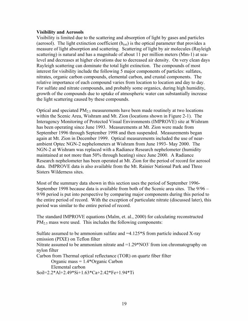
Visibility and AerosolsVisibility is limited due to the scattering and absorption of light by gases and particles(aerosol). The light extinction coefficient (bext) is the optical parameter that provides ameasure of light absorption and scattering. Scattering of light by air molecules (Rayleighscattering) is natural and has a magnitude of about 11 per million meters (Mm-1) at sea-level and decreases at higher elevations due to decreased air density. On very clean daysRayleigh scattering can dominate the total light extinction. The compounds of mostinterest for visibility include the following 5 major components of particles: sulfates,nitrates, organic carbon compounds, elemental carbon, and crustal components. Therelative importance of each compound varies from location to location and day to day.For sulfate and nitrate compounds, and probably some organics, during high humidity,growth of the compounds due to uptake of atmospheric water can substantially increasethe light scattering caused by these compounds.

Optical and speciated PM2.5 measurements have been made routinely at two locationswithin the Scenic Area, Wishram and Mt. Zion (locations shown in Figure 2-1). TheInteragency Monitoring of Protected Visual Environments (IMPROVE) site at Wishramhas been operating since June 1993. Measurements at Mt. Zion were made fromSeptember 1996 through September 1998 and then suspended. Measurements beganagain at Mt. Zion in December 1999. Optical measurements included the use of near-ambient Optec NGN-2 nephelometers at Wishram from June 1993- May 2000. TheNGN-2 at Wishram was replaced with a Radiance Research nephelometer (humiditymaintained at not more than 50% through heating) since June 2000. A RadianceResearch nephelometer has been operated at Mt. Zion for the period of record for aerosoldata. IMPROVE data is also available from the Mt. Rainier National Park and ThreeSisters Wilderness sites.

Most of the summary data shown in this section uses the period of September 1996-September 1998 because data is available from both of the Scenic area sites. The 9/96 –9/98 period is put into perspective by comparing major components during this period tothe entire period of record. With the exception of particulate nitrate (discussed later), thisperiod was similar to the entire period of record.

The standard IMPROVE equations (Malm, et. al., 2000) for calculating reconstructedPM2.5 mass were used. This includes the following components:

Sulfate assumed to be ammonium sulfate and =4.125*S from particle induced X-rayemission (PIXE) on Teflon filterNitrate assumed to be ammonium nitrate and =1.29*NO3- from ion chromatography onnylon filterCarbon from Thermal optical reflectance (TOR) on quartz fiber filter

Organic mass = 1.4*Organic CarbonElemental carbon

Soil=2.2*Al+2.49*Si+1.63*Ca+2.42*Fe+1.94*Ti

20

Reconstructed mass allows for a comparison of assumed forms of chemical combinationsof the elements to the total measured mass and tests the assumptions made.

PM10 mass was measured at Wishram (Teflon filter), but not at Mt. Zion.

As ammonium ion was not analyzed for, it is not known if the sulfate and nitrate werefully neutralized. At times significant concentrations of sodium and chloride ion werereported.

Scatterplots of reconstructed versus measured fine mass for Wishram and Mt. Zion areshown in Figure 2-9. About 90% of the fine mass is accounted for at both sites, andsquared correlation coefficients (r2) are about 0.9.

Figure 2-9. Measured versus reconstructed mass, Wishram and Mt. Zion 9/96-9/98.

Mt. Zion 9/96-9/98y = 0.91xR2 = 0.87

0

5000

10000

15000

20000

25000

0 5000 10000 15000 20000 25000

Measured fine mass (ng/m3)

Rec

onst

ruct

ed fi

ne m

ass

(ng/

m3)

Wishram 9/96-9/98 y = 0.87xR2 = 0.90

0

5000

10000

15000

20000

25000

30000

0 5000 10000 15000 20000 25000 30000

Measured fine mass (ng/m3)

Rec

onst

ruct

ed fi

ne m

ass

(ng/

m3)

21

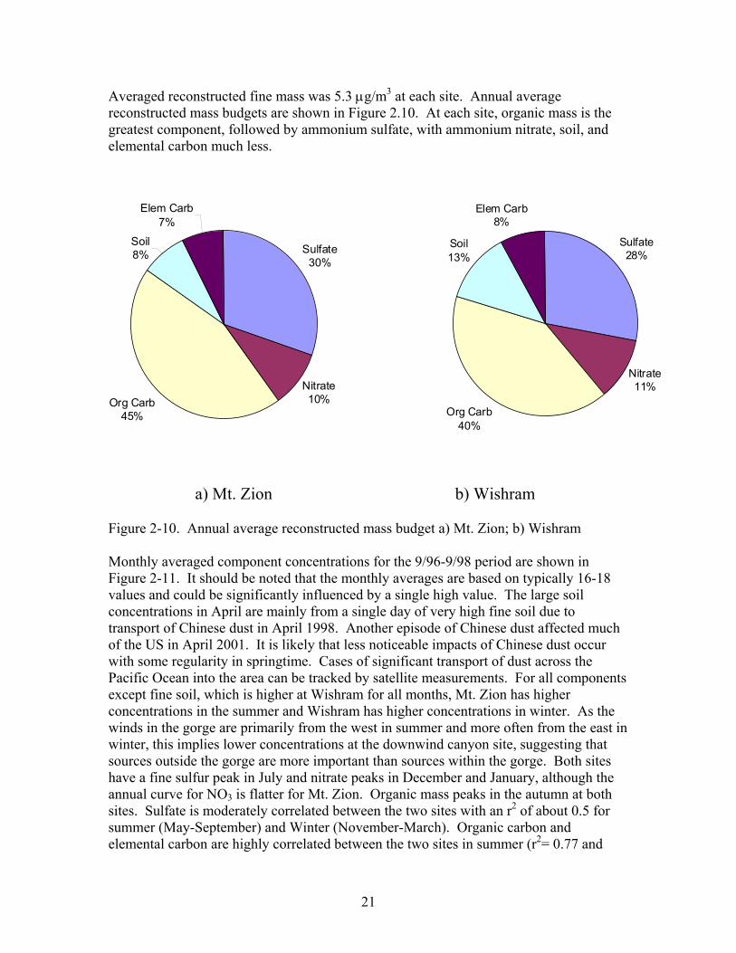
Averaged reconstructed fine mass was 5.3 µg/m3 at each site. Annual averagereconstructed mass budgets are shown in Figure 2.10. At each site, organic mass is thegreatest component, followed by ammonium sulfate, with ammonium nitrate, soil, andelemental carbon much less.

a) Mt. Zion b) Wishram

Figure 2-10. Annual average reconstructed mass budget a) Mt. Zion; b) Wishram

Monthly averaged component concentrations for the 9/96-9/98 period are shown inFigure 2-11. It should be noted that the monthly averages are based on typically 16-18values and could be significantly influenced by a single high value. The large soilconcentrations in April are mainly from a single day of very high fine soil due totransport of Chinese dust in April 1998. Another episode of Chinese dust affected muchof the US in April 2001. It is likely that less noticeable impacts of Chinese dust occurwith some regularity in springtime. Cases of significant transport of dust across thePacific Ocean into the area can be tracked by satellite measurements. For all componentsexcept fine soil, which is higher at Wishram for all months, Mt. Zion has higherconcentrations in the summer and Wishram has higher concentrations in winter. As thewinds in the gorge are primarily from the west in summer and more often from the east inwinter, this implies lower concentrations at the downwind canyon site, suggesting thatsources outside the gorge are more important than sources within the gorge. Both siteshave a fine sulfur peak in July and nitrate peaks in December and January, although theannual curve for NO3 is flatter for Mt. Zion. Organic mass peaks in the autumn at bothsites. Sulfate is moderately correlated between the two sites with an r2 of about 0.5 forsummer (May-September) and Winter (November-March). Organic carbon andelemental carbon are highly correlated between the two sites in summer (r2= 0.77 and

Sulfate28%

Nitrate11%

Org Carb40%

Soil13%

Elem Carb8%

Sulfate30%

Nitrate10%Org Carb

45%

Soil8%

Elem Carb7%

22

0.76, respectively), but not well correlated in winter (r2=0.37 and 0.14), as seen in Figure2-12.

Figure 2.11 Monthly average reconstructed fine mass components Wishram and Mt.Zion, September 1996-September 1998 a) Ammonium sulfate and ammonium nitrate; b)organic mass, elemental carbon, soil.

0

500

1000

1500

2000

2500

3000

3500


Con

cent

ratio

n (n

g/m

3 )

Mt. Zion AmmSO4 Wishram AmmSO4Mt Zion AmmNO3 Wishram AmmNO3

0

500

1000

1500

2000

2500

3000

3500


Con

cent

ratio

n (n

g/m

3 )

Mt. Zion soil Wishram soil Mt. Zion ECWishram EC Mt Zion OMC Wishram OMC

23

Figure 2-12. Scatterplots of organic mass and elemental carbon for Wishram and Mt.Zion, summer and winter.

Reconstructed fine particle extinctionReconstructed fine particle extinction is a method used to estimate the fractionalcontribution from each of the major aerosol components (sulfate, nitrate, organic carbon,elemental carbon, and crustal) to visibility impairment. Reconstructed fine particulatelight extinction by month is shown in Figure 2-13. Scattering by coarse mass was notincluded because coarse mass concentrations are not available for Mt. Zion. Themethodology included extinction efficiencies of 10 m2g-1 for elemental carbon, 4 m2g-1

for organic mass, 1 m2g-1 for fine soil and 3 m2g-1*f(RH) for ammonium sulfate andammonium nitrate, where f(RH) is a relative humidity growth factor. Daily averagedf(RH) was calculated from hourly f(RH) values for hours with RH of 98% or less. Thef(RH) is 1 below about 30% RH and then increases gradually at first, but then at an everincreasing rate which is quite rapid above about 90% RH (see Malm et. al., 2000 for thef(RH) growth curve and more detail). Wishram has higher particle scattering in themonths November to February, while Mt. Zion is higher the rest of the year. The

Summer (May-Sep) OMCy = 0.86xR2 = 0.77

0100020003000400050006000700080009000

10000

0 2000 4000 6000 8000 10000 12000

Mt. Zion OMC

Wis

hram

OM

CSummer (May-Sep) EC y = 0.90x

R2 = 0.76

0

200

400

600

800

1000

1200

1400

1600

0 200 400 600 800 1000 1200 1400 1600

Mt. Zion EC

Wis

hram

EC

Winter (Nov-Mar) OMC y = 0.61x + 919.21R2 = 0.37

0

1000

2000

3000

4000

5000

6000

7000

0 1000 2000 3000 4000 5000 6000 7000

Mt. Zion OMC

Wis

hram

OM

C

Winter (Nov-Mar) EC y = 0.48x + 295.81R2 = 0.14

0

200

400

600

800

1000

1200

0 200 400 600 800

Mt. Zion EC

Wis

hram

EC

24

considerably higher reconstructed extinction at Mt. Zion compared to Wishram insummer is due to both higher concentrations of most aerosol components and greaterwater growth of sulfate and nitrate than at Wishram due to higher humidity at Mt. Zion.

Figure 2-13. Average reconstructed particle extinction by month, Wishram and Mt. Zion9/96-9/98.

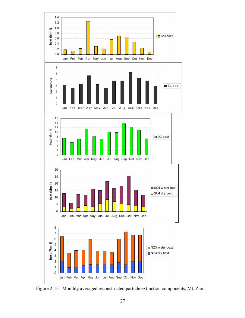
The monthly components of reconstructed extinction for Wishram and Mt Zion areshown in Figures 2-14 and 2-15. Estimated scattering due to dry particles and watergrowth of sulfate and nitrate is shown separately to emphasize the importance of watergrowth on scattering in the Scenic Area. At Wishram, it is interesting to note thatreconstructed sulfate extinction peaks in winter due to water growth, even though sulfateconcentrations are higher in summer. The nitrate extinction is less than 2 mm-1 insummer and 12 mm-1 in winter at Wishram. Organic aerosol is the greatest singlecomponent in summer at Wishram. Mt. Zion has less variation in extinction componentsduring the year as compared to Wishram. This is due to greater aerosol mass in thesummer and relatively higher humidity than Wishram in summer (less RH variation thanWishram between summer and winter).

Wishram & Mt. Zion average reconstructed fine particle extinction by month

0

10

20

30

40

50

60


reco

nstr

ucte

d fin

e pa

rtic

le

extin

ctio

n (M

m-1

)

Wishram Mt. Zion

25

Figure 2-14. Monthly averaged reconstructed particle extinction components, Wishram.

0.00.20.40.60.81.01.21.41.61.8


bext

(Mm

-1)

Fine soil bext

0

1

2

3

4

5

6


bext

(Mm

-1)

EC bext

0

2

4

6

8

10

12

14


bext

(Mm

-1)

OC bext

02468

101214161820


bext

(Mm

-1)

SO4 w ater bext

SO4 dry bext

0

2

4

6

8

10

12

14

Jan Feb Mar A pr May Jun Jul A ug Sep Oct Nov Dec

bext

(Mm

-1)

NO3 w ater bext

NO3 dry bext

27

Figure 2-15. Monthly averaged reconstructed particle extinction components, Mt. Zion.

0.0

0.2

0.4

0.6

0.8

1.0

1.2

1.4


bext

(Mm

-1)

Soil bext

0

1

2

3

4

5

6

Jan Feb Mar A pr May Jun Jul A ug Sep Oc t Nov Dec

bext

(Mm

-1)

EC bex t

02468

10121416

Jan Feb Mar A pr May Jun Jul A ug Sep Oc t Nov Dec

bext

(Mm

-1)

OC bex t

0

5

10

15

20

25

30


bext

(Mm

-1)

SO4 w ater bext

SO4 dry bext

0

1

2

3

4

5

6

7

8


bext

(Mm

-1)

NO3 w ater bext

NO3 dry bext

29

Measured versus reconstructed scattering at Wishram

A scatterplot of measured versus reconstructed particle scattering at Wishram for theperiod 9/96-9/98 is shown in Figure 2-16. Coarse mass (PM10-PM2.5) scattering wasincluded here, with an efficiency of 0.6 m2g-1. The same data organized by month isshown in Figure 2-17. Here, only hours with measured relative humidity of 90% or lesswere used with the requirement of at least 12 hours per day of data meeting thislimitation. At very high values the nephelometer shows extreme numbers; this was doneto avoid using these numbers. It should also be noted that the uncertainty in the RH datais 5%, so a value of 95% could actually be 100% RH.

Figure 2-16 Measured versus reconstructed particle light scattering, Wishram – 9/96-9/98.

Figure 2-17 Measured and reconstructed particle light scattering by month, Wishram 96/96-9/98.

Wishram measured vs recon bsp

y = 0.41x + 15.35R2 = 0.76

0

20

40

60

80

100

120

140

0 50 100 150 200 250 300

meas bsp

reco

n b s

p

Wishram measured vs reconstructed bsp

0

10

20

30

40

50

60

70

80


b sp (

Mm

-1)

bsp recon bsp

30

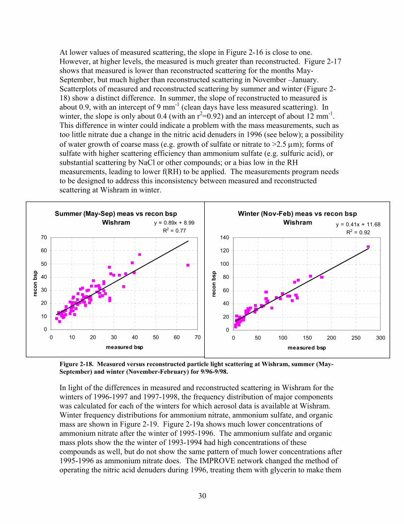
At lower values of measured scattering, the slope in Figure 2-16 is close to one.However, at higher levels, the measured is much greater than reconstructed. Figure 2-17shows that measured is lower than reconstructed scattering for the months May-September, but much higher than reconstructed scattering in November –January.Scatterplots of measured and reconstructed scattering by summer and winter (Figure 2-18) show a distinct difference. In summer, the slope of reconstructed to measured isabout 0.9, with an intercept of 9 mm-1 (clean days have less measured scattering). Inwinter, the slope is only about 0.4 (with an r2=0.92) and an intercept of about 12 mm-1.This difference in winter could indicate a problem with the mass measurements, such astoo little nitrate due a change in the nitric acid denuders in 1996 (see below); a possibilityof water growth of coarse mass (e.g. growth of sulfate or nitrate to >2.5 µm); forms ofsulfate with higher scattering efficiency than ammonium sulfate (e.g. sulfuric acid), orsubstantial scattering by NaCl or other compounds; or a bias low in the RHmeasurements, leading to lower f(RH) to be applied. The measurements program needsto be designed to address this inconsistency between measured and reconstructedscattering at Wishram in winter.

Figure 2-18. Measured versus reconstructed particle light scattering at Wishram, summer (May-September) and winter (November-February) for 9/96-9/98.

In light of the differences in measured and reconstructed scattering in Wishram for thewinters of 1996-1997 and 1997-1998, the frequency distribution of major componentswas calculated for each of the winters for which aerosol data is available at Wishram.Winter frequency distributions for ammonium nitrate, ammonium sulfate, and organicmass are shown in Figure 2-19. Figure 2-19a shows much lower concentrations ofammonium nitrate after the winter of 1995-1996. The ammonium sulfate and organicmass plots show the the winter of 1993-1994 had high concentrations of thesecompounds as well, but do not show the same pattern of much lower concentrations after1995-1996 as ammonium nitrate does. The IMPROVE network changed the method ofoperating the nitric acid denuders during 1996, treating them with glycerin to make them

Summer (May-Sep) meas vs recon bsp Wishram y = 0.89x + 8.99

R2 = 0.77

0

10

20

30

40

50

60

70

0 10 20 30 40 50 60 70

measured bsp

reco

n bs

p

Winter (Nov-Feb) meas vs recon bsp Wishram y = 0.41x + 11.68

R2 = 0.92

0

20

40

60

80

100

120

140

0 50 100 150 200 250 300

measured bsp

reco

n bs

p

31

more effective at removing gaseous nitric acid. This time frame coincides with anapparent reduction in particulate nitrate at Wishram. If the new method is correct, itsuggests a significant positive artifact occurred until 1996 (nitrate levels too high). If theolder method was more correct, the post- 1996 nitrate values could be too low. This iscurrently being investigated by the IMPROVE program. Additional measurements in theColumbia River Gorge could help resolve this issue locally.

Figure 2-19. Frequency distribution of reconstructed fine ammonium nitrate, ammonium sulfate,and organic mass at Wishram for the winters of 1993-94 through 1998-1999. The winter of 1994-1995 was missing most data.

Wishram Ammonium NO3 winter (Nov-Feb)

0

2000

4000

6000

8000

10000

12000

0 10 20 30 40 50 60 70 80 90 100Percentile

Am

mN

O3 (

ng/m

3)

W 93-94

W 95-96

W 96-97

W 97-98

W 98-99

Wishram Ammonium SO4 winter (Nov-Feb)

0

1000

2000

3000

4000

5000

6000

7000

0 10 20 30 40 50 60 70 80 90 100

Percentile

Am

mS

O4 (

ng/m

3) W 93-94

W 95-96

W 96-97

W 97-98

W 98-99

Wishram Organic M ass winter (Nov-Feb)

0

1000

2000

3000

4000

5000

6000

7000

8000

9000

10000

0 10 20 30 40 50 60 70 80 90 100

Percentile

OM

C (n

g/m

3) W 93-94

W 95-96

W 96-97

W 97-98

W 98-99

32

Long-term Ozone Field StudiesOzone is measured at only one site (Wishram) in the Scenic Area. Ozone measurementshave been recorded at Wishram since 1993. The temporal pattern at Wishram is typicalof an urban transport site. Median values fluctuated between 20 and 42 ppb. Since theozone levels do not typically dip below 20 ppb during the night hours, probably due toinsufficient nitrogen oxide (NO) to react with all of the ozone available, the dosagesobserved at Wishram are generally higher than those observed at urban or urban fringesites.

Peak one-hour averages occur during the mid-day and evening hours, and correlate wellwith regional ozone values. During episodic conditions when other sites in the regionexperience high ozone values, the observations at Wishram are also high. Wishram peakvalues are slightly higher than analogous sites located in pristine areas or national parksin the northwest (Olympic National Park and Mt. Rainier National Park), but lower thanprotected areas elsewhere in the west such as Sequoia/ Kings Canyon National Park.Wishram has never exceeded the 125 ppb one-hour ozone standard.

A single exceedance of the eight-hour average standard occurred at Wishram on July 13,1996. The July 1996 episode resulted in exceedances throughout the region. The site isin attainment of the 8-hr standard since the standard is computed as the average of the 4th

highest annual 8-hr average over three years. Since the ozone levels observed at Wishram have met, and continue to meet the nationalambient air quality standards, human health-related effects are not assumed to be an issuein the area that the site is representing. Wishram is considered a regional scale site(representative radius of over 50km). Measurements are not available for the west andcentral areas of the Scenic Area.

Sites in Portland have exceeded the 8-hr ozone standard 101 times between 1977 and2000. The probability of Portland sites exceeding the 8-hr standard on any given threeyears has been calculated to be close to 50%. This value may be slightly high due topotential bias from measurements conducted in the late seventies. EPA standardizedinstrument calibration procedures in 1980.

Special Ozone Studies During the summer of 1996 Cooper and Peterson measured the spatial variation in ozone

dosages in various transects throughout western Washington including the ColumbiaRiver Gorge. They deployed passive ozone samplers along nine river drainages fromnear sea level to mountain passes and other high altitude sites. They found that weeklyaverage ozone concentrations were highest in the drainages east and southeast of thegreater Seattle-Tacoma area (maximum = 55 to 67 ppb) and in the Scenic Area east ofPortland (maximum = 59 ppb).

In the case of the Columbia River Gorge transect, ozone dosages were higher withincreasing distance eastward in the Gorge with the exception of the western-most site.The western-most site, located 36 km east of Portland, had a higher summer averagedosage (32 ppb) than the two sites east of it (23 and 25 ppb) located 48 and 71 km east

33

from Portland. The highest summer average dosage was observed at Wishram (41 ppb).Although the highest weekly dosage was measured at Wishram, it is quite possible thatsites west of Wishram might experience higher peaks than Wishram. More availability ofNO at sites west of Wishram would lead to the disappearance of ozone at night, and thusresulting in lower weekly averages, but potentially higher daytime peaks, at sites closer tothe Portland urban area.

No air pollution modeling studies specific to the Scenic Area have been conducted.However, the western portion of the Scenic Area has been included in the 5-kmresolution modeling domain that Washington State University and Department ofEcology have been using since 1996. During the Southwest Washington Ozone study, avery considerable amount of effort was required to obtain an MM5 solution with reducedsurface wind speeds and wind directions congruent with observations in the Portlandarea. The complex terrain of the Scenic Area is a dominant topographical feature thatgreatly influences the flow patterns in that region. Since then, investigators at Universityof Washington (Sharp) have produced higher resolution MM5 runs of the gorge. Theresults they have obtained seem promising, but have not yet been verified withobservations mainly due to the sparse or non-existence of meteorological fieldmeasurements in the region.

3 HYPOTHESES TO BE TESTED

In this section, hypotheses are stated as a framework (or a basis) to plan a measurement,data analysis, and modeling program to help answer key questions regarding haze in theScenic Area. The hypotheses could just as easily be listed as a series of questions. Theyare used as a guide to designing the study, but not as the sole reason for making proposedmeasurements or conducting modeling and data analysis activities. Some analyses thatmust be done, such as closure (mass, optical, etc.) exercises, are not necessarily evidentin the list of hypotheses, but will be done.

HYPOTHESIS 1: In the summer and early fall, visibility in the gorge, in particularthe west end is significantly impacted by the Portland, Oregon/Vancouver,Washington metropolitan and to a lesser extent other regional sources(Kelso/Longview, Centralia powerplant, Seattle/Tacoma, Vancouver B.C.).

Evidence to support hypothesis 1: The Portland,Oregon/Vancouver WashingtonPrimary Metropolitan Statistical area (PMSA) had an estimated population on July 1,1999 of 1,845,840 (U.S. Census Bureau). The PMSA is immediately to the west of theColumbia River gorge. There are substantial quantities of particulates and precursorgases in the PMSA which could contribute to haze in the Gorge. During the summermonths, lower level winds are consistently channeled into the Gorge from the Portlandurban area due to a pressure gradient across the gorge. Temperature gradients betweenthe cool waters of the Pacific Ocean and heated interior areas east of the CascadeMountains results in a significant west-east pressure gradient. The Columbia River gorgeprovides a channel through which this pressure gradient can be realized, with the

34

resultant flow from high pressure to the west to lower pressure in the east. These windseffectively bring polluted air from the urban and industrial areas upwind into the gorge.

In addition to the flow from Portland, emissions from areas downriver (and upwind)along and near the Columbia River such as the Longview/Kelso area can be carried intothe gorge. Less frequently, emissions from areas north of the Columbia River such as theCentralia power plant and the Puget Sound to Vancouver, British Columbia region can becontributing to the mix due to northwesterly synoptic scale flow around the summertimePacific High.

More specific evidence of contribution of nearby sources west of the gorge in summer isgiven by diurnal plots of light scattering at Mt. Zion using a Radiance heatednephelometer. Figure 3-1 shows a regular diurnal pattern in light scattering in the monthsJune- October, with a sharp rise in bsp in late morning, a peak early in the afternoon andthen a decline. It is speculated here that the rise in late morning is due to transport of a“blob” of polluted air that had built up during light wind conditions overnight. As theheating of the interior increases the pressure gradient in the late morning, the windsincrease and move the blob through the gorge. Bsp decreases later in the afternoon due toincreased vertical and along-wind dispersion, and more rapid air-flow through thePortland area itself, limiting the buildup of pollutants that are subsequently transportedthrough the gorge.

Additional information needed: Additional monitoring can help confirm the effects ofthe Portland area and regional sources upon aerosol concentrations and visibility in the

Figure 3-1. Hourly averaged light scattering at Mt. Zion for June-October and November-May. Datafor the period 9/96-9/98. Light scattering measured by Radiance Research nephelometer withhumidity limited to 50% by heating.

Mt. Zion monthly averaged nephelometer by hour

10

15

20

25

30

35

0 2 4 6 8 10 12 14 16 18 20 22 24

Hour

bsp (m

m-1

)

Jun-OctNov-May

35

gorge during the summer. If the explanation for the diurnal patterns in light scattering atMt. Zion is correct, the diurnal peak in the heated nephelometer signal should be delayedwith distance downwind in the gorge. It is possible that the peak could be reducedsubstantially at locations downwind of Mt. Zion due to the pulse arriving during theperiod of maximum mixing. A nighttime peak should also be noted in the metropolitanarea. High time resolution light absorption data from aethalometers may also provide agood marker of the urban area and its associated emissions. High time resolutionparticulate sulfate and nitrate measurements may also be useful in identifying transport.Finally, 24-hour aerosol sampling and analysis could be useful by considering gradientsin aerosol concentrations.

As areas near, but above the gorge would be expected to be less influenced by thePortland area, nephelometer, aethalometer, and aerosol measurements at these areas canbe compared to those within the gorge to estimates the regional versus Portland areainfluences. This would tend to underestimate the Portland influence somewhat becausewhile much material from Portland/Vancouver is expected to enter the gorge, somematerial will be transported up slopes on either side of the gorge and up the sidewalls ofthe gorge itself (mainly the south-facing Washington side). By comparing withmeasurements further from Portland, a better indication of regional versus localcontributions can be made.

The measurements, in particular, those with time resolution of one-hour or less shouldhave collocated wind speed and direction to help define the source-receptor relationships.

At a minimum, measurements should be made upwind of Portland (between Portland andLongview/Kelso), in Portland, and at multiple distances downwind of Portland.Measurements at a clean location near the mouth of the Columbia River could provide anestimate of background levels.

Aircraft measurements of light scattering could also test this hypothesis. Airborneobservations could provide additional information on aerosol concentration gradients inrelation to boundary-layer and flow structure. By making several passes over the areawithin the gorge, these measurements could also provide insight into the possibletransport of pollutants up the slopes on either side of the gorge. It is suggested thatboundary layer growth and the subsequent mixing will act to reduce aerosolconcentration further downwind in the gorge. Airborne observations would be able todirectly test this hypothesis by making measurements at several altitudes.

Lidar could also be used to characterize aerosol concentration, distribution, and velocitythrough a cross-section of the gorge. Tetroons could be released from various locationsin the Portland/Vancouver area during midday in summer to see if they are transportedinto the gorge or are transported up slopes on either side of the gorge.

36

Transport and dispersion models would be helpful to show the potential for contributionsfrom more distant areas such as Seattle and Vancouver, B.C.

HYPOTHESIS 2: Visibility in the gorge, in particular, the east end is significantlyimpacted by urban and industrial sources in or near the gorge plus regional sourcesnorth and east of the gorge in the Columbia River basin in winter

Evidence to support hypothesis 2: Occasionally during winter, high pressure areas set upover the intermountain west, resulting in light winds over the Columbia River basin.Mixing heights are low and low clouds and fog are common in the gorge and ColumbiaRiver Basin providing an environment conducive to the formation of secondary aerosol.Pollutants accumulate and drift slowly into the gorge via drainage flows, where localsources add to the pollutant mix, resulting in the potential for significant buildup ofpollutants as well as formation of secondary aerosols. Drainage flow would slowlytransport pollutants down the Columbia River. Toward the west end of the gorge, the airaccelerates, with winds becoming strongest near the exit of the gorge. Automated ASOSvisibility measurements indicate widespread reduced visibilities in the area, commonlyincluding the Tri-Cities (Richland-Pasco-Kennewick), The Dalles, Yakima, andPendleton, and occasionally extending to Spokane. Near and east of the Scenic Area isthe Boardman coal-fired powerplant and nearly collocated feedlots. Within the gorge arethe towns of The Dalles (estimated population 12,175 and Hood River estimatedpopulation 20,400 (population estimates for July 1, 2000 from Portland State Universitypopulation research center). There are also some small industrial sources in the gorgeincluding aluminum smelters.

Additional information needed: Comparing aerosol and light scattering data along withwind speed and direction from monitoring sites on upwind and downwind side of townsin the gorge would give a good indication of the importance of their contribution to hazein the gorge. Light scattering and aerosol chemistry should be collected. Aethalometersmay also be useful in identifying periods of impact from the towns (diesel, wood-burning). A few additional aerosol monitoring sites at rural areas in the Columbia Riverbasin would be useful at determining the spatial consistency of the aerosol. Finally,monitoring sites near, but above the gorge would be useful in testing the hypothesis thatsubstantial aerosol is being channeled down the gorge. Sites should be located both nearthe Columbia River and away from the river to see if concentrations are higher along theriver. Differences in aerosol concentration and light scattering within and above thegorge could give an estimate of the contribution from sources in the gorge and areaswithin the Columbia River basin whose emissions drain into the gorge. Measurements offog chemistry could also help determine the role of fog and clouds in secondary aerosolproduction. Tetroons could be released from various locations in the Columbia RiverBasin during winter to see if they are transported into the gorge.

Aircraft observations could also help mapping out the 3 dimensional structure of aerosolsin the area, as described under hypothesis 1. Low clouds and fog could limit aircraftobservations in winter, however. Lidar could also be used to characterize the verticaldistribution of aerosol and aerosol transport as a function of height in the gorge.

37

Transport and dispersion modeling may be helpful to evaluate the potential forcontributions to winter haze from regions north and east of the gorge, such as theSpokane area.

HYPOTHESIS 3: SO2 and NOX emissions from the Boardman coal-fired powerplant just east and south of the gorge interact with ammonia from adjacent feedlots, in the presence of frequent low clouds and fog in winter to produce significantquantities of ammonium sulfate and ammonium nitrate that then moves into thegorge under drainage and larger scale pressure gradient flows.

Evidence to support hypothesis 3: The Boardman powerplant is a coal-fired unitoperated by Portland Gas and Electric and located about 15 km south of the ColumbiaRiver about 100 km east of the Scenic Area boundary. The powerplant is rated at560MW and is uncontrolled for sulfur dioxide. 1999 annual emissions included 16,578tons of SO2 and 8949 tons of NOX (Oregon DEQ). There is a feed-lot immediatelyadjacent to the Boardman plant; a few kilometers away is another feed-lot. These feed-lots have emissions of ammonia that would help in the formation of secondaryammonium nitrate and ammonium sulfate. During winter, fog and low clouds arecommon. This would be expected to result in enhanced secondary aerosol formation.During these conditions, winds are light; drainage flow and the mesoscale pressuregradient could cause the sulfate and nitrate formed by the interaction of the powerplantand feed-lot emissions to be transported into the Scenic Area. During a site visit to theplant in early January 2001, the top of the stack was in cloud. In the absence of sufficientammonia, but ample moisture, sulfuric acid and nitric acid aerosol would be formed.These would have the potential to cause ecosystem damage.

Additional information needed: More information is needed to estimate the magnitudeof aerosol produced by the Boardman plant and whether the aerosol is transported intothe Scenic Area. One method to determine conclusively if pollutants from the Boardmanplant are transported into the gorge would be through the use of artificial tracers, such ascertain perfluorocarbons. These materials could be released continuously from the plantduring winter conditions that are likely to cause transport into the gorge and monitoringfor the presence of these tracers in the gorge. This method also would give the dispersionfactor of emission from the plant, which could be used to estimate maximum possibleimpacts from the plant. Measurements of sulfate and nitrate at the tracer locations couldbe analyzed to see if sulfate and nitrate levels in the presence of tracer is higher thansulfate and nitrate at nearby sites without tracer. The difference would be an estimate ofthe impact of the power plant. This method called Tracer -Aerosol Gradient InterpretiveTechnique (TAGIT) by Kuhns, et. al. (1999) has been used for the Project MOHAVEtracer study (Green, 1999) and will likely be used in the Big Bend Regional Aerosol andVisibility Observational (BRAVO) study (Green, et. al, 2000).

In the absence of perfluorocarbon tracers, enhanced meteorological monitoring in theregion near the plant in conjunction with meteorological and trajectory modeling could beused to identify periods of likely transport of the emissions into the gorge. Aerosol

38

measurements at various locations surrounding the site could be established to see ifgradients exist between the upwind and downwind locations. Coarse PM may need to bemonitored as well as fine due to the large amount of water growth associated with theaerosol (See hypothesis 4). It may also be desirable to collect and chemically analyze fogin the area near the plant. It would be worthwhile to investigate whether any endemictracers are available, such as selenium, that would help determine the presence or absenceof emissions from the plant in ambient samples. Also, high-time resolution sulfate andnitrate monitors mounted on aircraft could be used to map out 3-dimensional sulfate andnitrate concentrations in the vicinity of the plant.

Air quality modeling using a mesoscale meteorological model such as MM5 along with achemical transport model could also be used to investigate the effects of the Boardmanpowerplant on air quality within the NSA. Additional meteorological monitoring using aradar wind profiler near the powerplant would help in providing the initial transportdirection for the plume in the modeling analysis.

Tetroons could also be released to follow air flow from the vicinity of the power plant.They could be set to follow air motion at estimated plume height. If tetroons releasedfrom near the plant travel though the gorge, plant emissions would also. These would bereleased on a forecast basis.

HYPOTHESIS 4: Following the evaporation of fog, sulfur and nitrogen containingaerosol droplets are too large to enter the IMPROVE PM2.5 sampler, but arescattering much light, causing an apparent inconsistency between measured andreconstructed scattering in the eastern portion of the gorge (Wishram monitoringsite).

Evidence to support hypothesis 4: In winter months, the nephelometer measuredscattering is substantially higher than scattering reconstructed from the aerosol data andusing the standard IMPROVE equations. Some, but not all of the difference can beexplained by the presence of fine sodium and chlorine. NaCl is very hygroscopic andthus quite effective at light scattering in humid conditions. We have no speciated PM10measurements. It seems likely that there is a significant amount of NaCl and NaNO3 inthe coarse mode (in the BRAVO study, NaNO3 was mainly coarse). There is commonlyfog and low clouds in the Columbia River gorge in winter. After the evaporation of fog,much of the hygroscopic aerosol may be in the coarse mode. Using the standard coarsemass scattering efficiency of 0.6 m2g-1 could significantly underestimate coarse particlescattering under these conditions. Additional information needed: Aerosol and light scattering measurements need to bemade on the same size particles for comparability. Nephelometers with a PM2.5 size cutinlet can be compared with the IMPROVE PM2.5 speciated data. PM10 samples should becollected on the same substrates as are now collecting PM2.5 and then fully speciated(elements, ions, OC/EC). Both PM2.5 and PM10 need to be analyzed for ammonium ionas well to help determine the chemical form of the nitrogen and sulfur containingcompounds. PM10 cut nephelometers can then be compared to the PM10 scattering data.

39

Finally, a nephelometer without a size-selective inlet can be used to determine if anysignificant scattering by particles >10 µm is being measured. Ambient (unheated)nephelometers should be used to determine the scattering in each size range. Addingheated nephelometers would give an idea of the importance of water growth for each sizerange. Optical particle counters would give an estimate of the particle size distributionfor particles greater than about 0.3 µm in diameter. More sophisticated measurementswould include ramping humidity up and down and measuring the particle sizedistributions and light scattering at each humidity level. Finally, it would be informativeto perform chemical analysis of fog water. This should include PH measurements todetermine if the fog is acidic or not.

HYPOTHESIS 5: Sources within the gorge are only minor contributors to aerosoland haze in the gorge.

Evidence to support hypothesis 5: Figure 2-8 showed average monthly estimatedaerosol major components for the Mt. Zion and Wishram monitoring sites. It is notedthat for the months November through February, during which winds in the gorge arefrequently easterly (from east to west), component concentrations are higher at Wishram,which is the upwind site in the gorge. Similarly for the period May through October whenthe wind are predominately westerly, component concentrations (except fine soil) arehigher at the upwind site (Mt. Zion). Thus, an argument can be made that becauseconcentrations decrease downwind within the gorge, sources within the gorge cannot becontributing significantly to the aerosol and haze levels in the gorge. It can also beargued that the Mt. Zion and Wishram sites are affected by nearby sources whoseinfluence would decrease significantly with distance downwind due to dispersion; if notfor sources within the gorge, concentrations would decrease even more between theupwind and downwind sites. Scatterplots of aerosol component concentrations showedmoderate relationships between the two sites, suggesting a significant regionalcomponent to the aerosol. Mt Zion and Wishram ammonium sulfate for summer (May-September) and Winter (November-March) had squared correlation coefficients (r2) isabout 0.5 for each. For OMC and EC, the 2 sites are highly correlated in summer(r2=0.77 and 0.76, respectively for OMC and EC), but poorly correlated in winter(r2=0.37 and 0.14 for OMC and EC)(see Figure 2-9). This suggests that regional sourcesof OC and EC are most important in summer, while local source of OC and EC areimportant in winter.

Additional information needed: A good emissions inventory can help identify sourcesthat may be significant. Major point sources are reasonably well documented, but somesources such as trains and ships, and highway emissions are not well documented.Emission estimates from area sources such as Hood River and The Dalles could beimproved upon as well. After review of emissions and other data, additional monitoringcould address the hypothesis. Upwind and downwind monitoring of cities within thegorge could give an estimate of their potential effects on gorge visibility. Additionalmonitoring within the cities would give an estimate of the amount of aerosol or lightextinction within the cities caused by local versus transported emissions. Speciatedaerosol measurements and light scattering and light absorption would be appropriate

40

measurements. It is recognized that for secondary aerosol, the full effect of emissionsmay be some distance downwind due to the time required for gas-to-particle conversion.

For trains and highways within the gorge, if the emission inventory indicates that thesesources may be significant, high time resolution monitoring with aethalometers andnephelometers very close to these sources can give an idea of their importance, at leastfor primary particulate emissions.

The effects of significant sources of SO2 within the gorge, such as aluminum smeltersmay be difficult to determine from monitoring due to the conversion time typicallyneeded for secondary aerosol formation. During winter conditions with low clouds andfog, conversion may occur sufficiently quickly to be able to detect impacts nearby usingspeciated aerosol measurements upwind and downwind of the sources.

Modeling emissions from sources within the gorge using high-resolution meteorologicalfields and emissions inventory and a chemical transport model could also be used toestimate effects from in-gorge sources. The model results need to be compared withmeasurements to obtain confidence that the emissions inventory and meteorologicalfields are well described.

HYPOTHESIS 6: Smoke from wildfires, prescribed fires, agricultural burning, andhome heating occasionally causes significant visibility degradation in the gorge andsurrounding areas.

Evidence to support hypothesis 6: Smoke contains substantial quantities of organicaerosol. Wildfires in the Pacific Northwest are most common in the late summer.Prescribed fire (reduced in scope in recent years) typically occurs in spring and late fall.Agricultural burning in the Willamette Valley and Columbia River Basin in autumn andwood burning for winter heating in cities in and near the gorge results in potentialimpacts from smoke nearly year-round. Occasionally large spikes are seen in organic(and elemental) carbon concentrations. There is no other likely explanation for thesespikes other than being due to fire. Core (2001) found moderate correlations betweenpotassium and organic carbon at Wishram and Mt. Zion. The best relationship betweenK and OC (r2=0.74) was for Mt. Zion under east wind conditions (winter). This could bedue to wood burning for home heating particularly in cities in the gorge such as HoodRiver and The Dalles, or other vegetative burning. The high correlation between Mt.Zion and Wishram for summertime OC and EC (r2=0.76 and r2=0.77) could behypothesized to be from burning affecting both sites during the same sampling period.

Additional information needed: It is critical to make measurements that can give us agood estimate of the importance of wood smoke and other major source types to organiccarbon. The reconstructed extinction analysis indicates that organic carbon is asubstantial contributor to haze in the Scenic Area. Analysis of aerosol organic carbon byGas Chromatography Mass Spectroscopy (GCMS) can give estimates of OC fromburning, diesel engines, gasoline engines, and meat cooking (Fujita et. al., 1998). The

41

methodology includes Chemical Mass Balance (CMB) modeling based upon the relativeabundance of various organic compounds identified in the GCMS analysis.

A substantial amount of organic material is needed for the GCMS analysis. This maynecessitate using material from a number of different samples to get a composite for say aweek of every day sampling or a month for every third day sampling. Another approachis to collect high-volume samples or multiple collocated samples, combining all samplesfor a day for one analysis. This sampling and analysis should be done for at least twosites- most likely Wishram and Mt. Zion. In addition, carbon-14 analysis could be doneto determine the contemporary versus fossil carbon ratio.

HYPOTHESIS 7: Organic aerosols, a major component of fine mass in the gorge,do not have significant fraction that are hygroscopic. The substantial enhancementof scattering during high humidity conditions is mainly due to water growth ofsulfur and nitrogen containing compounds.

Evidence to support hypothesis 7:Whether or not a significant fraction of the organic aerosol exhibits water growth duringhigh humidity conditions is very important in determining the extinction budget in thegorge. This is because while the concentration of organic compounds is estimated to beon average 40-50% higher than that of sulfur compounds (without water), the watergrowth of sulfur compounds causes the estimated extinction to be substantially greater. Ifa significant portion of the organic aerosol grows, then the relative importance of organicaerosol to light extinction could be significantly greater than is assumed in the instance ofno water growth. Typically, most organic compounds are considered to be hygrophobicrather than hygroscopic (Malm et al., 2000). Indeed, the presence of organic materialmay in some cases act to prevent water growth of particles containing sulfur and organicsboth. Using statistical analysis among light scattering, a systematically varying RH, andaerosol speciation, Malm and Day (2001) concluded that organic compounds in theatmosphere are essentially hygrophobic. Saxena et. al., (1995) using results fromTandem Differential Mobility Analyzer (TDMA) analyses at two sites concluded organicaerosols may enhance or inhibit water growth. Mc Dow et al. (1994) found that woodsmoke particles increased in mass by 10% as humidity increased from 40-90%, and founddiesel exhaust to increase only 2-3% in mass with the equivalent increase in RH.

Additional information needed: High time resolution aerosol speciation data, alongwith nephelometer data with systematically controlled RH would allow a statisticalapproach such as by that by Malm and Day with higher time-resolution. Using a high-time resolution carbon analyzer (about 1 hour), in conjunction with high time resolutionsulfate and nitrate analyzers would allow frequent measurements to be used to comparewith light scattering as a function of RH. For example, if short-term changes in organiccarbon concentration occur without a change in sulfate or nitrate, the scattering efficiencyof the added organic carbon can be estimated. These efficiencies can be compared over arange of relative humidities to see if the efficiency increases with higher humidity. Also,use of particle size counters such as optical particle counters and differential mobilityanalyzers can be utilized in conjunction with the nephelometers and high-time resolution

42

aerosol data to see if the distribution of particle sizes changes with different RH’s.Again, the trick is to separate out effects of sulfate and nitrate particle growth.

HYPOTHESIS 8: The existing IMPROVE sites (Wishram and Mt. Zion) aregenerally representative of the eastern and western portions of the gorge and notunduly influenced by nearby sources. The sites are also generally representative ofconditions below the rim of the gorge.

Evidence to support hypothesis 8: This hypothesis is significant in that, as the only sitesmonitored to date in the gorge, analyses and preliminary conclusions to date depend onthe area of representation for these sites. Also, the suitability of using these sites forlong-term trend analysis representative of the gorge as a whole depends upon the zone ofrepresentation of these sites. The siting of the sites is not in very close proximity to anysignificant sources. The sites are located 100-200 m above the river, and well below therim of the gorge. They are not in very close proximity to any highway or railroad,although these sources are located below the sites. Mt. Zion is located relatively close tothe Portland/Vancouver area and a pulp mill near the western end of the gorge, but not invery close proximity. Wishram is located approximately 15 km from The Dalles, but thisagain is not particularly close. As far as being generally representative of conditionsbelow the rim, there is no data at different elevations above the river. Hypothesis 9(below) states that due to strong winds, conditions are well mixed below the rim, whichwould support the contention that the sites are representative of conditions below the rim.However, without vertical soundings, we do not know the depth of the mixing.

Additional information needed: To determine if local sources are significantlyaffecting the site, additional monitoring on either side of the sites and high-timeresolution monitoring at the sites are useful. If aethalometer data (for example) for a siteshows spikes on 5-minute data, it is likely that local sources are impacting the site. Also,if local sources are affecting a site significantly, a site some distance downwind shouldshow a considerable reduction in impact due to dispersion. Monitoring should also bedone above and below the site to see the vertical scale of representation for the site. Easyto operate, relatively inexpensive high time resolution monitors such as nephelometers oneither side and above and below the site could help show the scale of representation ofthe site. High time resolution aerosol, such as nitrate, sulfate, and carbon, andaethalometer data could indicate what sources may be affecting the site by the temporalvariation of each aerosol component. In additional full speciation at locations on eitherside of the site may be useful to help identify the impacts of certain sources with uniquemarkers as well as giving an idea of the general area of representation for the site.

HYPOTHESIS 9: Air within the gorge is vertically well mixed year-round. Insummer, it is typically capped by an inversion which results in the primarytransport of outside air into the gorge via the east and west ends with little enteringfrom above.

Evidence to support hypothesis 9: Hypothesis 9 is formulated mainly on theory, ratherthan observations, because there are no observations available. Adiabatic mixing from

43

turbulence associated with the strong winds in the gorge may be expected to result inwell-mixed conditions within the gorge, with a capping inversion above. Additionally, insummer, a subsidence inversion associated with the Pacific High would enhance thestability above the gorge, resulting in little mixing of air from inside and outside of thegorge. Air inside the gorge would be mainly affected by what enters the gorge from theeast or west, depending on flow direction. An exception would be air entering frommajor side canyons, such as the Hood River.

It could be argued that there is significant mixing of air out of the gorge due to heating ofthe south-facing slopes on the Washington side. Upslope flows would enhance the exitof air from the gorge. It is important to resolve this issue in order to formulate conceptualmodels of regional source impacts and evaluate numerical transport and dispersionmodels.

Additional information needed: Upper-air meteorological data is needed to helpdetermine vertical transport and mixing properties in and above the gorge. Radiosondeswill give vertical profiles of temperature, dew point, wind speed, wind direction, andpressure. This enables us to see if a capping inversion is present at the top of the highwind layer or elsewhere. A limitation to radiosondes is that they only give informationfor the times they are released. Also during strong winds, the balloon may travelsignificantly in the horizontal as well as vertical direction. Radar wind profilers givewind speed and directions averaged over layers about 60 m thick, starting about 100 mabove the ground. The instruments are automated, operate 24 hours a day and take littlemaintenance. Radio Acoustic Sounding System (RASS) used in conjunction with theradar gives vertical profiles of virtual temperature, but typically only up to 1 km or so,which may not be sufficient to see the inversions of interest. For lower level winds,Doppler sodar collocated with the radar gives more resolution to the winds in the lowerlayers. The dearth of upper-air sounding sites in the area (the closest site is Salem,Oregon) adds to the importance of adding upper air observations.

Near-surface wind and temperature measurements on the slopes of the gorge, particularlysouth-facing slopes would be useful to consider if significant material is exiting the gorgethis way. Nephelometers collocated with the meteorological measurements would alsoshow (as air begins to flow upslope) if the aerosol exiting the gorge has higherconcentrations than the air above. Significant differences in nephelometer readings oraerosol concentrations within and out of the gorge would indicate limited mixing aboveand below the gorge.

The additional meteorological measurements could also be used to evaluate and refinemeteorological models, which could then be used as input to a dispersion model to helpunderstand the 3 dimensional flow fields and mixing of air within and above the gorge.

The following hypotheses were suggested at the peer-review workshop on the“straw-man” study plan.

44

HYPOTHESIS 10: Short-term climate variability leads to significant variability inattribution analysis.

Evidence to support hypothesis 10: Weather patterns change significantly due to cyclessuch as El Nino, La Nina. These changes include changes in frequency of transport fromsources to receptors as well as changes in precipitation, and cloud cover that would alterchemical transformation and deposition. Attribution analysis performed for any one-yearor for special study periods, e.g. winter and summer intensive studies, must be put intocontext by comparing with longer term expectations.

Additional information needed: Ideally, the attribution analysis would provide anestimate of impacts for the study period, average impacts, and a range of impacts due toclimate variability. The analysis could be qualitative, semi-quantitative, or quantitative.The estimated frequency of specific source-receptor relationships for the study periodcould be estimated for additional years by considering transport frequency as predictedby models run for multiple years. However, these models are likely to be models such asHYSPLIT using relatively coarse meteorological data. Thus, biases could result. Moresemi-quantitative estimates could be made by looking a general frequencies of winddirections at long-term monitoring sites. E.g. if easterly winds in the gorge are 50% morefrequent during the study year than for a long-term average, then impacts from sources inthe eastern portion of the region are greater during the study year than long-termaverages, perhaps by 50%. In short, regardless of the methodology applied, it isimportant to place the study period into perspective regarding probable frequency andmagnitude of impacts from specific source areas.

HYPOTHESIS 11: Spatial variability of visibility is significantly affected byammonia variability. Reductions in SO2 may lead to increases in NO3 due toammonia limitation.

Evidence to support hypothesis 11: There is not evidence in the study area to supportor refute hypothesis 11. It is based on an assumption that in the area, or portions of thearea, ammonia gas is not present in sufficient quantities for reaction with nitric acid forformation of ammonium nitrate particles. Limitations of ammonia would also lead to lessthan complete neutralization of sulfate particles, such as sulfuric acid (H2SO4) andammonium bisulfate (NH4SO4), which have different light scattering effects than thefully neutralized ammonium sulfate ((NH4)2SO4). If SO2 is reduced, there could be lessammonia used in neutralizing sulfates, thereby freeing up additional ammonia forreacting with nitric acid (HNO3) to produce particulate nitrate.

Additional information needed: Measurements of ammonia and nitric acid are neededto see if the atmosphere is ammonia limited. Measurements of ammonium ion wouldalso be helpful to help determine the degree of neutralization of sulfate aerosol. Thesemeasurements should be used in conjunction with measurements of particulate nitrate andsulfate. Measurements at a few sites throughout the study area would be desired. Thesemeasurements could also support emissions inventory and chemical transport modelevaluations

45

HYPOTHESIS 12: Secondary organics from non-fire biogenic emissions is asignificant contributor to PM2.5 mass.

Evidence to support hypothesis 12: The Pacific Northwest is heavily forested and canbe expected to be a significant source of biogenic compounds. Some biogenic compoundsundergo chemical reactions that result in the formation of particles.

Additional information needed: Speciated aerosol and gas phase organic analysisshould be done to identify certain compounds associated with biogenic emissions. Forexample, alpha-pinene is emitted from forests typical of the Northwest. Themeasurements, in conjunction with receptor modeling can help to estimate the biogeniccontribution to organic aerosol.

HYPOTHESIS 13: Fugitive dust emissions are overestimated and carbon emissionsare underestimated.

Evidence to support hypothesis 13: Reconciliation between modeled concentrations offugitive dust and measurements consistently show that modeled concentrations are toohigh. While positive and negative biases occur in inventories of fugitive dust emissions,the net result is to overestimate emissions, particularly transportable emissions (Watsonand Chow, 1999). The effects of emission height and deposition are not well understoodfor ground-level fugitive emissions.

On-road vehicle measurements and CMB source apportionment has shown that motorvehicle emissions of carbon are underestimated, mainly due to underestimation ofemissions from high emitting vehicles (Watson et. al, 1998)

Additional information needed: For any modeling of the region that includes fugitivedust, time-resolved inventories that are reflective of meteorological condition and activitylevel need to be used. The inventories should use the best available methods forestimating transportable emissions rather than total emissions. The results also need to bereconciled with ambient measurements, including crustal contribution to PM10. Thisimplies chemical characterization of PM10 as well as PM2.5.

HYPOTHESIS 14: Side canyon flows are important from transferring material intoand out of the gorge and act as chemical reactors and reservoirs.

Evidence to support hypothesis 14: Particularly in the central and eastern gorge, thereare numerous side canyons. Some of these side canyons include rivers that drainsignificant areas. It is reasonable to expect that these side-canyons would help facilitatetransfer of air into and out of the gorge through drainage flow, upslope flows, etc. Airthat enters the side canyons from the main gorge could have a longer residence time inthe gorge area by being cut-off from the typical moderate wind speeds in the main gorgechannel. This additional residence time could provide for enhanced conversion of gas toparticles within the gorge area.

46

The Hood River Valley includes several towns and supports a large orchard industry,including emissions sources such as smudge pots. Additional side canyons contain smalltowns and associated emissions sources as well.

Additional information needed: Meteorological measurements should be made in sidecanyons to characterize these flows. This could include surface measurements,particularly for wind speed and direction, and upper air measurements with highresolution, such as sodars or tethersondes. Nephelometers collocated with the surfacemeteorology sites could give an idea of the visibility effects associated with the side-canyon flows. For areas with significant sources, such as the Hood River Valley,speciated PM2.5 monitoring may be appropriate. An aethalometer could identify effectsfrom smudge pots with high time resolution. Gas phase monitoring of precursorcompounds in conjunction with PM2.5 measurements could help to assess whetherenhanced secondary particle formation is occurring in the side-canyons.

HYPOTHESIS 15: Geogenic sources (e.g. volcanoes) are sometimes importantcontributors to haze in the gorge).

Evidence to support hypothesis 15: Active volcanoes can release large amounts of SO2to the atmosphere, which can then form particles and contribute to haze. Popocatepetl inMexico has been emitting on the order of 5,000-10,000 tons per day of SO2 over the pastfew years. At the Miyakejima volcano in Japan, SO2 emissions have ranged from 20,000to 130,000 t/d, with an average of 40,000 t/d from mid September 2000 to February 2001.The eruption of Mt. St. Helens, which is very close to the National Scenic Area, in 1980spewed an estimated 1 millions tons of SO2 into the atmosphere. Subsequent monitoringby the United States Geological Survey (USGS) indicated continued releases of SO2 intothe atmosphere in the years following the eruption. The USGS stopped monitoring SO2from Mt. St. Helens when emissions dropped to below 25 tons per day.

Additional information needed: Activity from active volcanoes needs to be consideredfor data analysis, emissions inventory and modeling. If volcanoes in the Pacificnorthwest become more active, the USGS will most likely make estimates of SO2 usingcorrelation spectroscopy (COSPEC) for total column SO2 and wind speed data. Ifneeded, COSPEC measurements at Mt. St. Helens or other northwest volcanoes could bemade in support of the study. The large emissions from volcanoes such as Miyakijimacould have a contribution to sulfate in the Columbia River Gorge. PM2.5 speciatedmeasurements should be made along the Pacific Coast at one or more sites to determinebackground concentrations of components (in particular sulfate) entering the studyregion. This will help in setting boundary conditions for chemical transport modeling aswell as aiding in data analysis. The coastal monitoring site(s) could also identifybackground levels of soil dust during periods affected by Asian dust storms, such as theApril 1998 episode.

HYPOTHESIS 16: Protecting visibility protects other air quality concerns, such asecosystems, cultural resources, etc.

47

Evidence to support hypothesis 16: To improve visibility, reductions in emissions ofprecursor gases such as SO2, NOX, and VOC’s are important. Reductions in primaryorganic and elemental carbon and fugitive dust would also help improve visibility. Manyof these emissions also may contribute to additional air quality impacts. Acidic aerosolscontaining sulfur and nitrogen can cause damage to ecosystems and cultural resources.Elemental carbon, or soot, could also impair cultural resources by coating surfaces. NOXand VOCs contribute to ozone concentrations. Thus, reducing emissions that result inparticulate matter will also help reduce other air quality impacts. One potential cause ofecosystem impacts, emissions of air toxics, would not be directly addressed under actionsdesigned for visibility protection.

Additional information needed: More information needs to be gathered to determinethe sensitivity of resources to gases and aerosols. At a minimum, aerosol and cloud/fogwater acidity should be determined for sensitive areas. Resources should be monitoredfor evidence of adverse effects. Emissions inventories must include reasonable estimatesof toxic compounds.

HYPOTHESIS 17: Ozone concentrations throughout the gorge are currently wellbelow the national ambient air quality standard, and so are below levels of concernfrom a human health standpoint.

Evidence to support hypothesis 17: The ozone data collected at Wishram over the pastseven years has not yet shown a violation of the ozone standard. The 75th percentile ofthat data set falls below 42 ppb hourly average and the 99th percentile falls below 66 ppb,both far below the 125 ppb one-hour standard. As pointed out in the previous section,only one exceedance (not a violation) of the eight –hour average 85 ppb standardoccurred at the site during the regional episode of July 11-14, 1996.

Additional Information needed: Ozone measurements are needed at the west end andthe central region of the Scenic Area. Many more exceedances of the 8-hour standardhave occurred at the Portland sites; therefore it is possible that hourly ozone peaks at thewest end and in the central part of the Scenic Area would be higher than at Wishram.The ozone dosage work conducted by Cooper and Peterson is also suggestive of this.

HYPOTHESIS 18: Ozone concentrations in part of the Scenic Area are above levelsknown to negatively impact ecosystem resources.

Evidence to support hypothesis 18: The fact that the 8-hr standard is apparently beingmet at Wishram would indicate that vegetation is being protected since the standard wasset both as a primary one (to protect human health) and as a secondary one (to protectpublic welfare including vegetation.) However, other evidence does not support thisindication. Although the 8-hr standard is expected to be more protective of vegetationthan the 1-hr standard, it does not directly account for cumulative exposure or maximumconcentrations. According to the Federal Land Managers’ Air Quality Related ValuesWorkgroup (FLAG), cumulative exposure and peak concentration are important

48

biological parameters. They propose the use of other ozone metrics such as the W126.The W126 is an index that uses a sigmoidal weighted function to weigh each hourlyozone concentration.

Native plant species sensitive to ozone were identified for different regions in the FLAGdocument and by Brace, Peterson and Bowers in their Guide to Ozone Injury in VascularPlants of the Pacific Northwest. Several of these ozone–sensitive species are found in theScenic Area, among them are western serviceberry (Amelanchier alnifolia), salal(Gaultheria shallon), Ponderosa pine, Quaking Aspen (Populus tremuloides). The ForestService has documented ozone damage to pine species at Maryhill State Park in theEastern Gorge. The FLAG document also points out that ozone can affect entire ecosystems as shown inU.S. EPA research in which plants growing in areas of high exposure to ambient ozonemay undergo natural selection for ozone tolerance.

Additional Information needed: Changes in growth and ecosystem form or function aredifficult to document. A field survey of sensitive plant species in the Scenic Area mightreveal any damage currently occurring due to ozone. As already suggested, at least twomore continuous ambient measurement sites in the Scenic Area are needed. An indexsuch as W126 using any existing and future continuous measurements should becomputed so that ozone exposure to vegetation in the Scenic Area can be betterevaluated.

HYPOTHESIS 19: Ozone measured within the Scenic Area results primarily fromprecursor emissions outside the Scenic Area and is tied to regional episodes.

Evidence to support hypothesis 3: The temporal pattern at Wishram is suggestive of a“transport site” as defined by Bohm et al. Transport sites are characterized by ozonemaxima in the late afternoon and early evening. At night the ozone levels typicallyremain above 20 ppb.

A precursory look at the data shows that ozone concentrations are elevated at Wishramwhen they are elevated at most other sites in Portland and throughout the region. Thisfact is not surprising in light of the unique set of meteorological conditions that areneeded to generate and sustain a high ozone episode: light winds and high temperaturesthat typically accompany strong high pressure ridges that can build off the coast in thesummertime. Recker (1997) and Steenburg et. al. (1996) have documented thesesynoptic conditions that lead to ozone episodes in Washington and Oregon.

Additional Information needed: As pointed out earlier, additional ozone monitors areneeded to get a better spatial picture of the ozone concentrations throughout the ScenicArea. At the Technical Foundation Study phase (TFS), with appropriate background andinitial data, a Lagrangian model using verified trajectories through the Scenic Area couldprovide a first look at ozone formation dynamics.

49

Regional Eulerian photochemical grid modeling is needed during episodic conditions tounderstand the spatial and temporal distribution of ozone in the gorge as well as itsprecursors. A modeling exercise of that nature is also needed for understanding theformation of secondary aerosols, and so would be an essential ingredient of an air qualitystudy in the gorge. Process analysis of the proposed grid modeling study will be useful tofollow the formation of the ozone plume and establish its main contributors.

HYPOTHESIS 20: Elevated ozone concentrations are correlated with periods ofimpaired visibility. Reductions in ozone precursors will have a positive benefit onvisibility.

Evidence to support hypothesis 20: The following theoretical evidence exists to supporthypothesis 20:

i. In the gas phase, oxidation of SO2, the initial step in the formation of sulfateaerosol, occurs predominantly through reaction with the hydroxyl radical (OH).OH production is enhanced during periods of peak ozone formation.

ii. Sulfur oxidation through reaction with ozone in the aqueous phase is rapid.iii. Ozone and OH aid the formation of secondary organic aerosol by the oxidation

of low vapor pressure organic gases.iv. Stagnant meteorological conditions with low vertical mixing are typical of ozone

episodes, and also lead to elevated concentrations of smog-related aerosols andNO2. NO2 is a gas that absorbs light, and, like aerosols, can also cause visibilityimpairment.

Additional information needed: A statistical analysis of periods of elevated ozone andthe corresponding measured light-extinction needs to be conducted. In addition, processanalysis of the modeling results to follow the atmospheric chemistry processes thatpredominate during periods of elevated ozone and impaired visibility in the Scenic Areawill help verify hypothesis 20.

50

4 ELEMENTS OF THE PROPOSED STUDY

There are three components in the study (monitoring, emissions inventory, andmodeling). This section outlines the various methods and approaches that are underconsideration. 4.1 MONITORING COMPONENT

In this section a list of measurements is presented. They correspond to the measurementsdescribed to support (or refute) the hypotheses, but are organized byinstrument/measurement type. In the subsequent section the order of priority for themeasurements is given along with the information added with each measurement and thecost. In some cases, additional measurements of the same type are called for at additionalsites (e.g. more aerosol gradient sites)

The measurements need to be designed to meet expected needs of quantitative sourceattribution models as well as in the development of conceptual models. This includesmeasurements to use for model input as well as for model evaluation. The measurements need to have an uncertainty associated with them. This is necessaryfor placing confidence in conclusions drawn from the data, for use in receptor modeling,and for evaluation of meteorological and chemical transport modeling. Assigninguncertainty to measurements is best determined by having a period of collocatedmeasurements in the study area, although collocated measurements done in otherlocations may be adequate. These measurements can give a quantitative value ofprecision, although accuracy is not directly addressed. At monitoring sites with both hightime resolution measurements and longer (e.g. 24 hour) average measurements, the high-time resolution measurements can be averaged to the 24-hour period for comparison.Additional aspects regarding measurement quality are addressed in Section 8- QualityAssurance.

Many of the measurements in the monitoring program will be conducted within theScenic Area and regions nearby. To the uninitiated this may appear to bias resultstowards in-Gorge sources. But because the Scenic Area is the receptor of pollutantsemanating from various regions near and far, it is very critical to know what is happeninginside the Scenic Area to be able to understand what, when and where the pollutantscome from.

4.1.1 Optical measurements

Nephelometers

Heated nephelometers or nephelometers used in conjunction with Nafion dryers will bedeployed as a sort of high time resolution aerosol monitor, while ambient nephelometerswill be used to characterize ambient light scattering. Heated nephelometers may

51

volatilize some aerosol, such as nitrate and volatile organics. It would be preferable touse dry scattering for example, with Nafion driers which would not volatilize aerosolcomponents, if resources allow. Both dry and ambient nephelometers will helpcharacterize the spatial and temporal patterns in the Scenic Area. These will be used inconjunction with meteorological data (especially wind speed and direction).

• Ambient nephelometers will give a measure of total light scattering including theeffects of water growth. Comparison with collocated heated nephelometers willgive an estimate of the importance of water growth. Ambient nephelometers arenecessary only at sites where a complete extinction budget is needed (e.g. Mt.Zion and Wishram). At these sites PM10 cut and PM2.5 cut ambient nephelometersshould be used in addition to open-air nephelometers in order to evaluate fine andcoarse particle scattering and compare to PM10 and PM2.5 chemical speciation.

• Nephelometers placed along the gorge will be used to identify effects of sourcesor source areas propagating through the gorge (e.g. the Portland urban plume) andto consider the effects of in-gorge sources (cities) by the differences in upwindand downwind light scattering (all year).

• Nephelometers placed at different vertical heights will give some understandingof the vertical distribution of aerosol in the gorge and how it

• changes on a diurnal or seasonal patterns or with different synoptic weatherconditions. It will help answer questions of whether material is mixed out of thegorge during the day or due to turbulence or whether material in the gorge staysconfined to the gorge (all year). A location in mid-gorge e.g. Cascade Locks ispreferred.

• Nephelometers placed in the Portland/Vancouver urban area and upwind ofPortland can give an idea of the increase in light scattering across the Portlandarea and presumably due to the urban area (mainly summer).

• Nephelometers placed at some distance (10-20 km away from the gorge on eitherside of an along river monitoring site east of the gorge can give an idea of whethermaterial is being channeled narrowly along the river, or is spread out horizontally(winter).

• RH controlled nephelometers with RH ramped up and down to see effect of watergrowth. These are most effective when used with high-time resolution aerosolspeciation data.

• Nephelometers mounted in aircraft could give information on vertical mixing ofthe aerosol and how distributions change with distance downwind in the gorgeand by time of day.

Aethalometers

Aethalometers measure light absorption through a filter tape. The measurements aretypically reported as mass concentration of black carbon, but can also be interpreted asambient light absorption. The measurements have time resolution of 5 minutes or moredepending upon ambient levels; thus they are useful in determining whether local sourcessuch as diesel emissions are affecting the site. They may also help identify impacts fromurban areas, which have elevated light absorption.

52

Aethalometers placed at the Mt. Zion and Wishram IMPROVE sites would identify anyimpacts from local sources and add to the characterization of the aerosol and opticalproperties of the sites. An aethalometer at Mt. Zion may indicate arrival of air from thePortland urban area. An additional aethalometer at a nephelometer and surfacemeteorology site between The Dalles and Hood River could help give an indication ofimpact from these towns.

Total light extinction

A measure of the total light extinction is desirable as a check on the light scattering andlight absorption measurements as well as being a measure directly related to haze. Thesum of scattering by gases and particles and absorption by gases and particles shouldequal the total light extinction. This comparison i.e. optical closure has proved somewhatelusive in the past. The absorption measurements typically have been based upon filter-based measurements which may not directly relate to atmospheric measurements. Photo-acoustic methods (e.g. Moosmuller) are a more direct measurement of absorption than arefilter-based measurements and include NO2 absorption as well (filter measurements donot). Light scattering measurements by nephelometers have scattering angle truncationeffects, which mostly results in missing a portion of the coarse particle scattering. Evenin near-ambient nephelometers, some modification of the aerosol occurs due to heating ofthe aerosol by the nephelometer lamp.

Transmissometers measure the total light extinction through a path in the atmospherefrom the light source to the receiver, typically a distance of a few kilometers. Thesemeasurements are hard to compare directly to nephelometer and various absorptionmeasurements, which are made at essentially one point, as are aerosol measurements.Also, the transmisssometer measurement relies on an accurate calibration of lampbrightness, which varies (in a somewhat predictable manner) over time. Density changesin the atmosphere due to large temperature gradients can cause broadening of the lightbeam, thereby increasing the measured extinction, even though it is unrelated to aerosolconcentration. During periods of fog and low cloud, common to the Scenic Area,transmissometer measurements may be either unavailable or indicating very highextinction (which, while correct, may be of little use). In spite of these limitations,transmissometers could be of potential use in optical closure, if sited such that thetransmissometer sight path is representative of the scattering and absorption measurementareas. It would be most useful for periods without low clouds or fog.

Total extinction measurements such as the extinction cell developed by Moosmuller mayprovide a better method than transmissometers for optical closure. The extinction cell,coupled with photo-acoustic absorption measurements and nephelometers (missing somecoarse scattering) could provide a good measure of each component of light extinction.NO2 measurements would give the required information to calculate its light absorption.

Ground based LIDAR

53

LIDAR uses the backscatter of light from aerosol to indicate the distribution of aerosolalong the beam. By rotating the beam, the aerosol distribution over a volume, as well asthe velocity of the aerosol can be determined. This can be very useful in understandingthe vertical mixing characteristics in an area and showing whether aerosol is beingtransported by certain features, such as nocturnal jets, etc. A LIDAR situated in mid-gorge may be most useful in documenting aerosol transport up and down the gorge.LIDAR will work only up to the base of clouds. Under clear conditions to above thegorge, information upon aerosol concentration and transport within and above the gorge,and whether there is coupling can be obtained.

4.1.2 Aerosol and Gaseous Measurements

As light scattering and light absorption by aerosols is the main cause of visibilityimpairment, aerosol measurements are critical to understanding haze, including thesource types and source areas responsible. A wide-variety of aerosol measurements areproposed, covering time-scale of minutes to a day and from chemical speciation of mostelements to identification of individual compounds and organic aerosol speciation. Aswith nephelometers, aerosol measurements can be used to determine gradients in thehorizontal and vertical, with high time resolution for some measurements. The addedbenefit of speciated aerosol measurements over nephelometers is identification of whichchemical components are changing in time or space. However, high time resolutionaerosol speciation is more costly and difficult than high time resolution light scatteringfrom nephelometers. High time resolution aerosol in conjunction with nephelometer datacan be very effective for assessing the causes of haze.

Gaseous measurements can help especially for the air quality models. SO2 in conjunctionwith SO4 measurements give a measure of the fraction of gas-to-particle conversion;VOC measurements can help in the evaluation of the air quality (chemical transport)models especially for secondary organic aerosol from biogenic emissions. Ammonia(NH3) is useful to help evaluate the emissions inventory and to determine availability ofammonia for full neutralization of SO4 and NO3 aerosol. NOy is of value for use inchemical transport modeling

Aerosol and gas measurements proposed include:

• PM2.5 and PM10 monitoring at Wishram and Mt. Zion with full chemicalspeciation. Currently PM10 is only done on Teflon and is not analyzed forchemical species. The monitoring should be done for one-year on the IMPROVEschedule and daily for intensive studies. The analysis should also include NH4and SO2, which are not currently done. These measurements are needed forcalculation of the extinction budget.

• Deployment of DRUM size-resolved impactors at a minimum of Mt. Zion andWishram, and one site outside the gorge representative of regional conditions.These can give 1-hour time resolution speciated aerosol in 3 or 8 size ranges.Sites need to be visited once per six weeks. Inexpensive sampling can be done

54

for long periods of time and analyzed later for exceptional events. Thesemeasurements, in conjunction with nephelometer data and meteorological datawill help in the identification of which sources impact a site at a given time. Thesite above the gorge will give the regional background. By comparison with thesites in the gorge, the regional versus transport through the gorge difference canbe obtained for each element. This could be quite useful for studying the effectsof Portland in the summer, for example. They also give information on size ofaerosol needed for Mie-theory calculations and will give additional informationregarding the water growth of aerosols.

• Organic speciation using GCMS at a minimum of Mt. Zion, Wishram, and onesite above the gorge. This, in conjunction with Chemical Mass Balancemodeling (CMB) will allow us to apportion organic aerosol to key source types(burning, diesel, gasoline vehicles, and meat cooking).

• Speciated aerosol at a few locations along the gorge, best if situated withnephelometers and surface meteorology sites. This will allow us to see howchemical component concentrations change with distance downwind in the gorge.If the ratio of the mix changes, then certain compounds must be added due tosources or chemical transformation (e.g. SO2 to SO4) (or selectively removed,which is less likely). This will help tell what sources in the gorge arecontributing.

• Speciated aerosol at river-level-mid gorge and top of gorge at a site in mid-gorgee.g. Cascade Locks. Useful in conjunction with collocated nepehlometers andsurface meteorology to evaluate vertical mixing in-gorge.

• Speciated aerosol in Portland (at least 3 sites) and upwind (minimum 1 site) insummer (minimum). Along with nephelometers, gives estimate of contribution ofPortland to gorge aerosol. Also, may provide source signature for Portland, ifsignificantly different from upwind sites.

• Speciated aerosol at multiple sites in Columbia River basin in winter. Givesinformation on spatial consistency of aerosol in Columbia River basin, which isoften upwind of gorge in winter. Could help identify contributions fromsignificant sources.

• High-time resolution SO4, NO3, EC/OC at Mt. Zion in summer and Wishramwinter (minimum). Can help evaluate local versus regional scale of impacts, ofsites, possibly identification of specific sources impacting sites, and could helpwith refining scattering efficiency and water growth factors when used with otherinstruments (e.g. wet/dry nephelometers or RH ramped nephelometers).

• Measurements of additional gas-phase compounds, especially NH3, HNO3, NOy,SO2, O3, and speciated organic gases. Useful for air quality modeling,determination of limited species for chemical reactions.

55

• Fog water sampling and chemical analysis during winter. Use to evaluate acidityof fog for possible ecosystem and cultural resource damage. May also be usefulto help understand aerosol properties and visibility effects when fog evaporates.

• Condensation particle counter, optical particle sizer, differential mobilityanalyzer. Deploy during summer and winter intensive studies. Determineparticle size (needed for theoretical scattering calculations). Used with high-timeresolution chemistry help to understand aerosol water growth. Largeconcentration of condensation nuclei indicates a nearby source. Particle sizemeasurements could also be taken aboard aircraft to give 3-dimensional structureof particle count and size distribution during periods of particular interest.

• Additional out-of-gorge IMPROVE monitoring sites will continue to routinelycollect speciated PM2.5 data. This includes site at Mt. Hood, The 3 SistersWilderness, Mt. Ranier, Snoqualamie Pass, and other IMPROVE monitoringsites. This data can help specify regional background conditions for the NSA.

4.1.3 Meteorological measurements

Meteorological measurements, especially wind speed and direction are needed tounderstand source-receptor relationships. Analysis of data from the measurements willhelp understand flows into and out of the gorge, including along side canyons, andvertical mixing. They are also necessary for input to and evaluation of meteorologicalmodels. They are useful for interpretation of other measurements such as light scatteringand speciated aerosol.

Proposed measurements include:

• Surface meteorology: wind speed, direction, temperature, relative humidity atmain aerosol monitoring sites and all nephelometer sites. Wind speed anddirection will help confirm the sources which may be contributing to themeasured light scattering or aerosol concentrations. RH is needed for estimatedwater growth used for reconstructed scattering calculations. Temperature atdifferent vertical levels in the gorge can give an idea of stability and verticalmixing of aerosol. Surface meteorological data can also be used for input to orevaluation of meteorological models.

• Radiosondes: Radiosondes give vertical profiles of horizontal wind speed anddirection, temperature, relative humidity, and atmospheric pressure. Radiosondesreleased within the gorge will give us information regarding the transport ofmaterial within the gorge. The temperature structure will indicate if cappinginversions are present that prevent mixing with material above the gorge. Alsovertical profiles of wind speed will help in estimated the speed of transport ofmaterial through the gorge. The radiosondes will also be helpful in evaluatingmeteorological models. Radiosondes should be released during typical summer

56

and winter conditions and 3 or more times per day to help capture diurnal cyclesin wind and thermal structure.

• Radar wind profilers with RASS and Sodar. Radar wind profilers typically givehourly averaged winds at intervals of 60 meters from about 100 m AGL to 5000m (or so) AGL. These operate continuously with little maintenance. As withradiosondes, they help understand vertical variations in the horizontal wind; theyalso give the vertical velocity component of wind. Radio acoustic soundingsystem (RASS) used in conjunction with the radar wind profilers give verticalprofiles of virtual temperature to about 1000 m. Similar to the radiosondetemperature data, information regarding vertical stability below about 1000 m canbe obtained. Sodars collocated with the radar wind profiler can give higherresolution wind data (horizontal and vertical) at low levels and is used tosupplement the radar wind profilers in the lower layers of the atmosphere. Aswell as helping to understand flow patterns and pollutant transport, hemeasurements can be used as input to meteorological models and to evaluate theperformance of the models. Radar wind profilers would be helpful in manyplaces. The number of profilers deployed would be limited by resources andsuitable locations for deployment. Desirable locations for profilers include: mid-gorge, western end of gorge, eastern gorge, near Longview, near Boardman, southof Portland.

• Ceilometers. Ceilometers are optical instruments that give the height of cloudbases. Cloud base height is useful for chemical transport modeling by serving asinput to or evaluation of the model predicted cloud levels. Chemicaltransformation processes are quite different if liquid water is present than in theabsence of liquid water.

• Solar radiation. Spectrally-resolved solar radiation is useful for calculation ofphotolysis rate parameters in chemical transport modeling.

4.1.4 Tracers

These measurements would track transport or transport and dispersion from emissionssources or source areas. They are also valuable in evaluating transport and dispersionmodels.

• Tetroons. Tetroons are constant pressure balloons that are tracked by radio. Thesefollow airflow and give an indication of where pollutants may travel. A tetroonreleased and set to flow at the height of a power plant stack may track thecenterline of the emissions from the plant. Release of multiple tetroons at alocation could give an estimate of horozontal dispersion. However, as thetetroons are confined to a set pressure (height), dispersion from vertical shear ofthe horizontal wind would not be properly realized. Still, it should give areasonable indication of whether emissions from a location where the tetroons arereleased would travel into the gorge. A prime candidate area for tetroon releases

57

would be near the Boardman coal-fired powerplant in winter. Also, potentialrelease sites would be in around the Portland area during summer to see howmany are transported into the Columbia River Gorge. Potential conflicts withaircraft would have to be addressed.

• Perfluorocarbon tracers. Perfluorocarbon tracers (PFT’s) are chemicalcompounds that have very low atmospheric background (generally <1 part perquadrillion). A release and ambient monitoring of these compounds gives thetransport and dispersion properties of the air into which it is released. They donot account for wet or dry deposition, or chemical conversion that will affect gasand particles in the atmosphere. When used successfully, they can be veryeffective at documenting the transport of emissions in to an area of interest as wellas giving the dispersion factor. These are very useful for evaluating transport anddispersion models as well. PFT’s could be injected into the stack of theBoardman powerplant in winter and monitored in the National Scenic Area to seeif the emissions from the plant are entering the gorge. Consideration of aerosolconcentrations gradients between where the plant emissions are noted by tracerconcentrations above background, and locations with no elevated tracer levelsgives a quantitative estimate of sulfate and nitrate due to the power plant (TAGITmodel).

58

In Table 4-1, the recommended measurements to consider are presented in order ofpriority.

Table 4.1 Recommended measurements to consider and estimated costs in order of priority.Measurement What it tells us Cost

Technical Foundation StudyAmbient nephelometers at Wishram, Mt.Zion – minimum 1 year

Light scattering including watergrowth effects

$30K+$18K/yr

Aethalometers at Wishram, Mt. Zion –minimum 1 year

High time resolution lightabsorption–impact of local sources?See Portland material movingthrough?

$24K/site +$10K/site/yr$68K 1year, 2 sites

Additional heated nephelometers withsurface meteorology along Gorge (3minimum e.g. Cascade Locks, anotherbelow Hood River, between Hood River &The Dalles) plus heated nephelometerswith surface meteorology at 3 verticallevels in mid-gorge (river, above river, rim)

Bsp gradient along gorge/effects oflocal cities. Vertical mixing/bspgradients

$20K+$15K/yr /site=$105K 3sites 1 year

Portable Radar wind profiler and/ortethersonde and ceilometer deployed at keyareas – e.g. mouth of gorge, mid-gorge,side canyons, eastern gorge for exploratorymeasurements + 1 year one site

Basic information on structure ofatmospheric flow in gorge – depth offlows, side-canyon importance, etc.Help to design more detailedmeteorological measurements

$100K

PM2.5 PM10 cut ambient nephelometers atWishram, Mt. Zion – 1 year

Fine and coarse particle scattering,comparison with PM2.5 and PM10speciation data

$88K+36K/yr

PM10 speciation at Wishram, Mt. ZionInclude NH4+, SO2 IMPROVE schedule, 1year

Speciation for comparison withcoarse particle scattering-aerosolneutralization

$30K+$70K/yr=$100K

NH3, HNO3 (g), SO2, Wishram, Mt. Zionone year IMPROVE schedule, 1 day in 6,4-6 samples per day for NH3, HNO3, SO2.Continuous NOy, O3

Provide data for air quality modelingDetermine if atmosphere is ammonialimited- evaluate emissionsinventory

$200K

Precipitation and Fog water sampling andchemical analysis- Boardman powerplantarea, central gorge as possible during 45day period

Determine potential ecosystem andcultural resources affects

$80K

Speciated PM2.5 east of Gorge (ColumbiaBasin) and west of the Gorge (upwind ofPortland). IMPROVE 1 day in 3 schedule.

Regional species gradient (transportsites) east and west of Gorge.

$60K/site, 2sites, 1 year= $120K

Scene Monitoring (Camera). Digital ImageAcquisition and Time Lapse Video. Twosites, one western and one eastern ScenicArea

Digital scene images to visuallyillustrate visibility conditions, andtime lapse video to capturedynamics of formation andmovement of haze.

$42K firstyear, $31Keach yearthereafter.

59

One-year expanded measurement program: additional horizontal and vertical gradients ingorge year-round, in-gorge vs. out-of gorge sources

Additional PM monitoring site collocatedwith mid-gorge nephelometer site.Speciated PM2.5 and PM10, with NH4+,NH3, SO2,

Characterize central gorge.Compare with measurements at eastand west end of gorge. Somegradient information.

$40K +$80K/yr=$120K 1-year

Gas and particle phase speciated organicaerosol using GCMS. 2 sites, one in sixdays for 1 year

Identification of key organic speciesin gas and particle phase.Contribution of biogenics, burning,gasoline, diesel, and meat-cookingto organic carbon with CMB

$160K

Radar wind profiler/SODAR/RASS 1 site,1 year

Vertical wind/temperature profiles $100K

Speciated PM2.5 2 nephelometer sites alonggorge- IMPROVE schedule, 1 year

Species gradient along gorge/localcity effects $30K+$80K

/yr=$110KDRUM samplers vertical nephelometersites 1 year, analyze periods of interest

Vertical gradients of species (at leastsulfur)

$75K

Speciated PM2.5 at nephelometer site at topof gorge, IMPROVE schedule, 1 year

In gorge/above gorge speciesgradient $15K+$40K

/yr=$55K2 Additional aethalometers either side ofCity of Hood River – year round

Help determine presence ofemissions from gorge cities,especially winter wood burning

$68K

High –time resolution SO4, NO3, EC/OC 1-3 sites (Wishram , Mt. Zion, mid-gorgesite) 1 year

Year-round knowledge of chemicalspecies changes in time $100K/site+

$100K/yrper site=$200-$600K

Summer intensive period studies – effects of Portland/VancouverContinue measurements as appropriate from TFS and one-year expanded network study and add:Nephelometers and surface meteorologyupwind (downriver) of Portland (one ormore), Portland (3)

Change in light scattering due toPortland urban area

$25K/site4 sites=$100K

Speciated aerosol upwind of Portland (3)/Portland (3), along gorge sites (5), top ofgorge (1 or more) Daily for 30 days July-August, reporting, meetings

Chemical speciation changes due toPortland urban area – relate to lightscattering changes

$140K+$110K/month (6new sites)

Radiosondes 4/day for 30 days 2 sites, onemid-gorge, one mouth of gorge (e.g. PDX)

Vertical profiles of stability and wind(mixing, transport speed)

$60K

High –time resolution SO4, NO3, EC/OCMt. Zion or central gorge site.

Chemical species change in time –relate to nephelometer data

$140K

DRUM samplers 5 along gorge sites 30days- analyze periods of interest

High-time res. speciation- Trackmovement of Portland plume

$50K

Radar wind profilers & sodars 6 sites Vertical wind profiles $200KOrganic gas and aerosol speciation, at Spatial pattern of organic speciation $100K

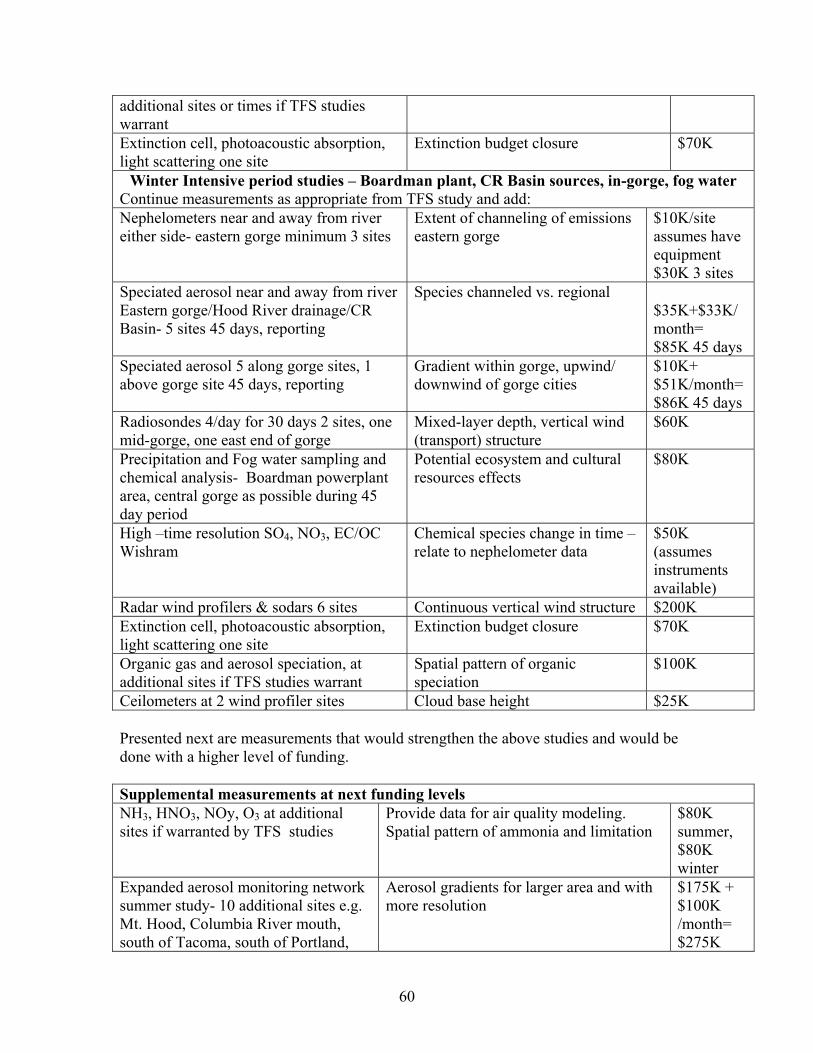
60

additional sites or times if TFS studieswarrantExtinction cell, photoacoustic absorption,light scattering one site

Extinction budget closure $70K

Winter Intensive period studies – Boardman plant, CR Basin sources, in-gorge, fog waterContinue measurements as appropriate from TFS study and add:Nephelometers near and away from rivereither side- eastern gorge minimum 3 sites

Extent of channeling of emissionseastern gorge

$10K/siteassumes haveequipment$30K 3 sites

Speciated aerosol near and away from riverEastern gorge/Hood River drainage/CRBasin- 5 sites 45 days, reporting

Species channeled vs. regional$35K+$33K/month=$85K 45 days

Speciated aerosol 5 along gorge sites, 1above gorge site 45 days, reporting

Gradient within gorge, upwind/downwind of gorge cities

$10K+$51K/month=$86K 45 days

Radiosondes 4/day for 30 days 2 sites, onemid-gorge, one east end of gorge

Mixed-layer depth, vertical wind(transport) structure

$60K

Precipitation and Fog water sampling andchemical analysis- Boardman powerplantarea, central gorge as possible during 45day period

Potential ecosystem and culturalresources effects

$80K

High –time resolution SO4, NO3, EC/OCWishram

Chemical species change in time –relate to nephelometer data

$50K(assumesinstrumentsavailable)

Radar wind profilers & sodars 6 sites Continuous vertical wind structure $200KExtinction cell, photoacoustic absorption,light scattering one site

Extinction budget closure $70K

Organic gas and aerosol speciation, atadditional sites if TFS studies warrant

Spatial pattern of organicspeciation

$100K

Ceilometers at 2 wind profiler sites Cloud base height $25K

Presented next are measurements that would strengthen the above studies and would bedone with a higher level of funding.

Supplemental measurements at next funding levelsNH3, HNO3, NOy, O3 at additionalsites if warranted by TFS studies

Provide data for air quality modeling.Spatial pattern of ammonia and limitation

$80Ksummer,$80Kwinter

Expanded aerosol monitoring networksummer study- 10 additional sites e.g.Mt. Hood, Columbia River mouth,south of Tacoma, south of Portland,

Aerosol gradients for larger area and withmore resolution

$175K +$100K/month=$275K

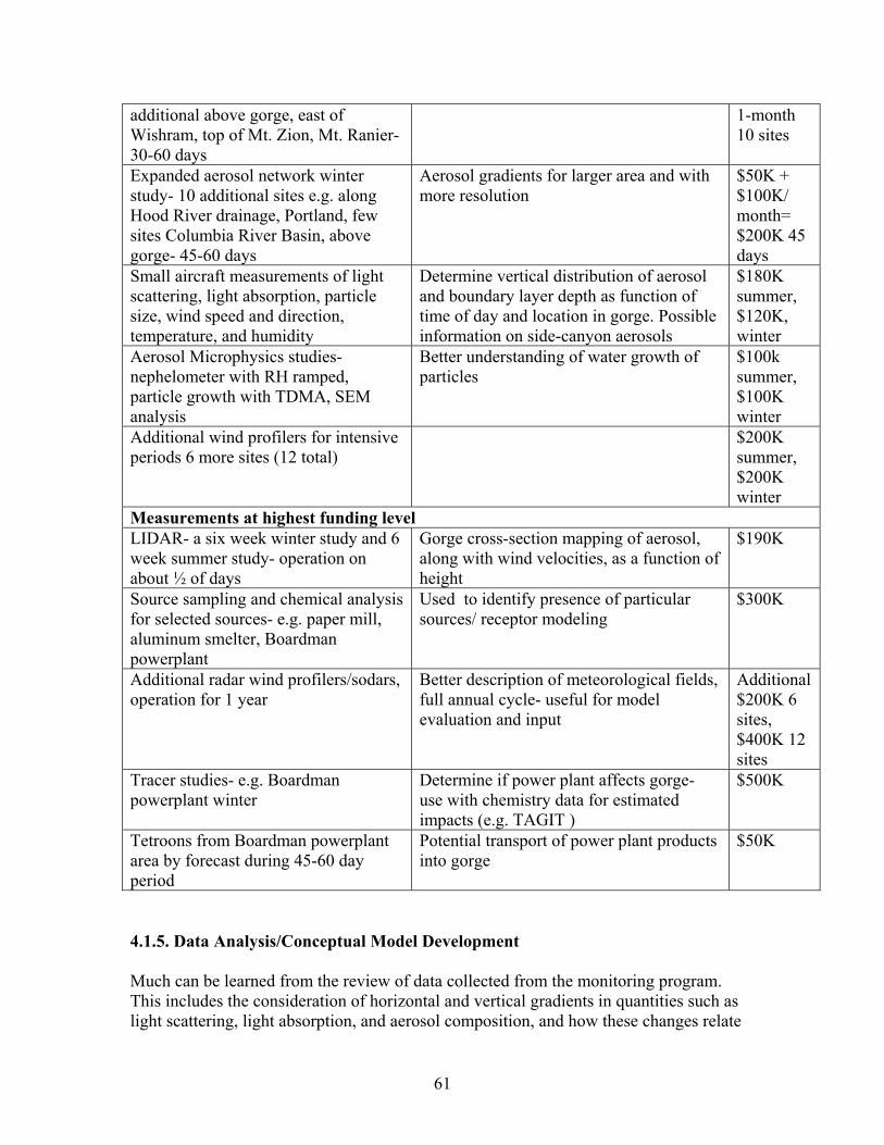
61

additional above gorge, east ofWishram, top of Mt. Zion, Mt. Ranier-30-60 days

1-month10 sites

Expanded aerosol network winterstudy- 10 additional sites e.g. alongHood River drainage, Portland, fewsites Columbia River Basin, abovegorge- 45-60 days

Aerosol gradients for larger area and withmore resolution

$50K +$100K/month=$200K 45days

Small aircraft measurements of lightscattering, light absorption, particlesize, wind speed and direction,temperature, and humidity

Determine vertical distribution of aerosoland boundary layer depth as function oftime of day and location in gorge. Possibleinformation on side-canyon aerosols

$180Ksummer, $120K,winter

Aerosol Microphysics studies-nephelometer with RH ramped,particle growth with TDMA, SEManalysis

Better understanding of water growth ofparticles

$100ksummer,$100Kwinter

Additional wind profilers for intensiveperiods 6 more sites (12 total)

$200Ksummer,$200Kwinter

Measurements at highest funding levelLIDAR- a six week winter study and 6week summer study- operation onabout ½ of days

Gorge cross-section mapping of aerosol,along with wind velocities, as a function ofheight

$190K

Source sampling and chemical analysisfor selected sources- e.g. paper mill,aluminum smelter, Boardmanpowerplant

Used to identify presence of particularsources/ receptor modeling

$300K

Additional radar wind profilers/sodars,operation for 1 year

Better description of meteorological fields,full annual cycle- useful for modelevaluation and input

Additional$200K 6sites,$400K 12sites

Tracer studies- e.g. Boardmanpowerplant winter

Determine if power plant affects gorge-use with chemistry data for estimatedimpacts (e.g. TAGIT )

$500K

Tetroons from Boardman powerplantarea by forecast during 45-60 dayperiod

Potential transport of power plant productsinto gorge

$50K

4.1.5. Data Analysis/Conceptual Model Development

Much can be learned from the review of data collected from the monitoring program.This includes the consideration of horizontal and vertical gradients in quantities such aslight scattering, light absorption, and aerosol composition, and how these changes relate

62

to meteorological conditions such as wind speed and direction, mixing, etc. The high-time resolution of one-hour or less proposed for some of the measurements, inconjunction with meteorological data and emissions information, will be illuminating asto the transport and mixing of visibility reducing aerosols affecting the Scenic Area.These analyses will be of considerable value in the formulation of conceptual models ofthe way in which emissions, meteorology, and visibility-reducing aerosol are related inthis region. These analyses will also be quite useful for aiding the selection, furtherdevelopment, and evaluation of quantitative models of source apportionment.

Many of the ways in which these measurements will be used for data analysis weredescribed in the hypotheses and measurements sections of this plan. Another way toorganize a discussion of data analysis is by the types of analysis.

Descriptive analysis includes a summarization of the data collected. Several purposesare served by descriptive analysis including data quality assurance and validation, datafamiliarity, and a means of testing the plausibility of some aspects of prospectiveconceptual models. An example of descriptive data analysis is summarizing temporaland spatial patterns of aerosol concentration.

Association analyses are similar to descriptive analyses except that more than oneparameter is considered at a time. Like descriptive analysis, association analysis is animportant step in data quality assurance and validation, promotes data familiarity, and is ameans to test conceptual models. In addition association analysis allows precision (andother quality descriptors) to be directly determined from collocated measurement, permitsassessment of aerosol and optical closure at some of the more complete monitoring sites,and may reveal insightful relationships concerning the conditions associated with andcauses of haze. They also test our assumptions of the reconstructed mass, scattering, etc.Examples of relevant closure exercises are presented below:

• Fine mass (PM2.5) and PM10 closure – compare the sum major of measured speciescombined with the mass of the assumed common oxides with the gravimetric fine andPM10 mass; should also include ion balance

• Optical closure – compare the sum of the measured light scattering and lightabsorption with the total measured light extinction; and

• Scattering, absorption, and extinction budgets – compare the sum of the calculatedscattering and extinction for the major aerosol components (component concentrationmultiplied by a scattering or extinction efficiency that may be a function of relativehumidity) with the measured total light scattering or extinction. For size-selectivemeasurements of scattering, absorption, or extinction (e.g. nephelometers with PM2.5inlets), compare with reconstructed scattering, absorption, or extinction from PM2.5aerosol component concentrations.

In order to know how applicable special study results are to other periods of times (othertimes of the year and other years), the representativeness of the study period must bedetermined. The approach used to determine representativeness of the study period startsby comparing meteorological and air quality data during the study period with similar

63

data for other times during the year and for the same period of time in previous years.Significant changes in emissions also need to taken into account when consideringrepresentativeness. Simple statistical tests and comparisons of frequency distributionplots for the study period and other periods show the degree of similarity of the studyperiod is to those other period for each parameter.

Once the data have been analyzed, the conceptual model of the physical and chemicalprocesses governing air quality in the Scenic Area will be developed.

64

4.2 EMISSIONS COMPONENT

A good emissions inventory is necessary to understand air quality, perform sourceattribution and evaluate alternative emissions scenarios. An emissions inventoryincluding SO2, NOX, NH3, speciated VOC, and speciated primary PM is needed. Thisincludes emissions from all potential source types affecting the gorge – industry, mobilesources (e.g. vehicles, ships, trains, air craft), area sources (e.g. woodstoves, outdoorburning, solvent use, agriculture), and biogenics (e.g. natural emissions from vegetation).Proper spatial and temporal distribution of the emissions is also necessary. Temporalresolution is normally hourly, and spatial resolution depends on analysis requirements. Inchemical transport models, emissions typically require the same spatial resolution as themeteorological data. Efforts are underway, as described below, to produce a “state of thescience” inventory for the Pacific Northwest; however, verification with measurementswill be necessary to evaluate how “good” the inventory really is.

Oregon and Washington have been involved in emissions inventory preparation for manyyears. Inventories have been prepared in response to federal and state requirements forpoint source reporting, State Implementation Plans (SIPs) for visibility and individualcriteria air pollutants, and various special studies. The states have a history ofcooperation, though coordinated inventory efforts have been fairly limited in scope. Withthe increased emphasis on regional issues such as ozone and haze, Idaho, Oregon andWashington initiated the formation of the Northwest Regional Technical Center(NWRTC). The NWRTC is tasked with the comprehensive analysis of transport,dispersion, and chemical transformation of airborne emissions throughout the PacificNorthwest, and will be instrumental in the development of Regional Haze SIPs. As partof the initial demonstration, the three states are meeting regularly to coordinate emissionsinventory efforts for two haze episodes that occurred in July 1996. The inventoryresulting from the demonstration project will be used as a basis for this proposed study.

The states began the inventory process by discussing a comprehensive list of sourcecategories that could potentially contribute to visibility impairment. Staff identified thesources believed to be the most significant contributors and assigned a lead from one ofthe states to each category. The leads are in the process of researching their sourcecategories and will make recommendations to the group addressing the pollutants,methodology, data sources, temporal/spatial resolution, and spatial surrogate. Sourcesare listed in the table below.

During discussion, the states found common inventory deficiencies. They requested andreceived special funding to inventory several of the source categories identified(woodstoves, residential outdoor burning, commercial marine vessels, railroads, andbiogenics). In addition to the regional inventory projects funded, Oregon received specialfunding to obtain stack parameters for point sources, inventory aircraft, researchammonia emission factors, and other work if resources allowed. Results from the fundedwork are expected during the summer of 2001.

65

NWRTC Emissions Inventory Source Categories and PollutantsCategory Include? PollutantsMajor Point Sources Yes criteriaOnroad Mobile Sources Yes criteria, NH3Locomotives Yes criteriaShips Yes criteriaAircraft state’s discretion criteriaRecreational Boats Yes criteriaOther Nonroad Mobile Yes criteriaResidential Wood Combustion Yes criteriaRestaurants further research criteriaAgricultural Burning Yes criteriaPrescribed Burning Yes criteriaOther Open Burning Yes criteriaWildfires further research criteriaAgricultural Tilling further research criteriaWindblown Dust further research criteriaPaved Road Dust Yes criteriaUnpaved Road Dust Yes criteriaSurface Coating Yes criteriaSurface Cleaning Yes criteriaCommercial/Consumer Products Yes criteriaBiogenics Yes criteriaLivestock NH3 Yes NH3Fertilizer Application Yes NH3Soil NH3 Yes NH3

Through the NWRTC, the emissions will be prepared for air quality modeling using theSparse Matrix Operator Kernel Emissions (SMOKE) emissions processor. Spatialsurrogates are being obtained and will be assigned to 12-km grids using GIS methods andincorporated into SMOKE along with temporal and chemical speciation profiles. TheNWRTC is carefully looking into the most recent research that the Western Regional AirPartnership (WRAP) has produced on fugitive dust sources, and will incorporate theirrecommendations into the emissions inventory.

It is worth noting that staff from the three states participate regularly in the EmissionsForum of the WRAP. WRAP is a Regional Planning Organization formed to address thefederal regional haze rules, and is made up of government, tribes, industry, andenvironmental groups throughout the western US. Technology transfer is part of theWRAP process, and the state modeling inventories are expected to benefit from theknowledge gained by WRAP.

The inventory process and resulting NWRTC inventory will be modified and enhanced tomeet the needs of the TFS study. This may involve adapting the inventory for a differentepisode, and could involve processing the data using a finer spatial resolution. Because

66

the spatial surrogates will be obtained in GIS formats, finer grid resolution will bepossible. Adapting the inventory to a different episode could require generating newemission rates for sources that vary with meteorology (onroad mobile, biogenic, etc.). Itcould also involve obtaining growth factors to project activity to other years.

Effects of control measures upon ambient concentrations of particulate nitrate can also betested using the Simulating Composition of Atmospheric Particles at Equilibrium(SCAPE) model (Kim et al., 1993a, 1993b) along with the proposed NH3, NH4

+, NO3-,HNO3, and SO4 measurements. The model apportions nitric acid/nitrate andammonia/ammonium between gas and particle phases. If the agreement with themeasurements is satisfactory, the model can then be applied to evaluate effects ofapplying controls to ammonia and/or total nitrate (gaseous + particulate) upon ambientparticulate concentrations. Another chemical model is needed to assess the effects ofNOX controls on total nitrate.

After the TFS effort, it is likely that more inventory work will be needed. Morecomprehensive source category coverage and spatial definition may be necessary. Thiscould involve special source surveys. Inventory verification involving additional gridmodeling for comparisons to measurements may be necessary. Additional work may alsoinvolve source sampling to help quantify certain emissions. Additional sourcecharacterization may be appropriate to establish source profiles for certain sources for usein Chemical Mass Balance (CMB) modeling. A review of source types present in thearea and the availability of appropriate source profiles for these sources should be made.Source sampling could then be done to generate source profiles for potentially significantsource types without appropriate existing profiles.

4.3 MODELING COMPONENT

As discussed above, there are two main objectives to the modeling component of thestudy:

1) to help understand current sources contributing to air pollution within the gorgethus supporting or modifying the conceptual model.

2) to provide a modeling methodology for future use in quantitatively estimating airquality changes resulting from different emissions scenarios.

Models can be used to help us understand some of the processes suggested by theanalysis of the air quality and meteorological monitored data. When a quantitative modelcan reasonably agree with the processes suggested by the conceptual model, the certaintyof our conclusions about both models is increased. The ultimate goal is a completemodeling system (emissions, meteorological fields, air quality model) that can accuratelyexplain the measurements and thus can, with some confidence, predict the future given avariety of emissions scenarios.

For the first objective, a model is used that will tell us how much of an impact we canattribute to a source or type of sources. There are several types of attribution models.Some work in a forward manner from emission sources to receptors (locations in the

http://www.wrf-model.org/

http://www.src.com/calpuff/calpuff1.htm

67

Scenic Area). These models work by taking a known mix of emissions, transportingthem by and through meteorological conditions, chemically transforming the pollutants,and finally depositing the resulting chemical species in the air or on the ground in thereceptor location. Other models work in the reverse. For these models, the sample at theend point (for example, from an IMPROVE or other monitoring site) is analyzed for itschemical constituents, and an attempt is made to match that composition with what weknow about the make up of a source category’s emissions. Essentially, each sourcecategory has a unique “finger print” that suggests that the source was responsible for allor part of the impact. Used alone, however, reverse attribution models in general canonly identify types of sources (e.g. pulp mills versus diesel vehicles versus coal firedboilers) rather than specific individual sources.

For the second objective, a model is used to predict future air quality usingmeteorological measurements, source specific pollutant emissions data, and calculated orassumed boundary conditions to calculate the transport, dispersion, deposition andchemical transformation of pollutants in the atmosphere. These predictive models can beused to predict future air quality impacts from a variety of emission scenarios.

It is possible that the same modeling system could be used for both objectives.

Because haze, ozone, and secondary particle formation operate on a regional scale, aregional scale modeling system is required. This eliminates the use of simple straight-line Gaussian plume models like the Industrial Source Complex (ISC) and AERMOD.

Most regional modeling systems have three components: an emissions model, ameteorological model, and an air quality model. Each component is briefly describedbelow.

4.3.1 Emissions Modeling

An emissions processor is necessary for converting emissions inventory data intoformatted emission files for the grid-type dispersion models. This process is describedabove in the emissions inventory component. Finer resolutions may be required for thefiner resolution (4, 1.33-km and potentially 0.4-km) grid structure. These activitieswould include GIS mapping of county level emissions to the grid, meteorologicaladjustments to the emissions, inclusion of any day-specific emissions (e.g., CEM data),temporal (e.g., day-of-week and diurnal) adjustments, and speciation into the species inthe chemical mechanism being used.

Limitations in emissions inventories will also affect modeling adequacy. Sources of SO2should be reasonably well quantified. NOX emissions estimates may also be reasonablygood. Higher uncertainties may be associated with the ammonia, particulate and VOCinventories. Measurement, data analysis, and receptor modeling components of the studymay be sufficient to characterize impacts from some of the sources contributing to theseinventories.

68

The modeling relies on an accurate knowledge of emissions of primary and precursorcompounds, an adequate representation of the meteorological fields (wind speed anddirection, turbulence, moisture, precipitation, etc.), and accurate treatment of chemicalreactions.

4.3.2 Meteorological Modeling

Most regional scale air quality modeling systems require time-varying three-dimensionalwind fields in order to simulate the complex spatial and temporal wind flows overmodeling domain (several hundreds of kilometers in size). These wind fields aretypically generated using meteorological models used in weather forecasting. Anexample of such a model is the Fifth-Generation NCAR / Penn State Mesoscale Model(MM5) model. Currently, it is reasonable to run these models using a relatively coarse(12 km) resolution grid over the entire Pacific Northwest (e.g., Oregon, Washington andIdaho). However, because the terrain within the Scenic Area is complex, narrow anddeep, a 12-kilometer grid spacing would not resolve much of the terrain within the ScenicArea. The use of such a coarse grid would smooth out much of the terrain features withinthe Gorge. A much finer grid resolution (perhaps less than 1 km) is need to adequatelyresolve the terrain so that the wind flow within the Gorge may be correctly simulated. Inthis modeling study, the modeling domain would likely need a nested grid structure suchas:• 36-km grid covering the western U.S. • 12-km grid covering Washington, Oregon, and western Idaho;• 4-km grid covering southern Washington, northern Oregon, and potentially extending

into most western Idaho;• 1.33-km grid covering the Columbia River Gorge region;• 0.44-km grid, if necessary, covering the Gorge area.

Three-dimensional grid modeling at the 36/12/4/1.33/(0.44)-km scales listed above arequite time and resource intensive, with most of the resources used in the finest grid areas.Therefore, it is expected that only a few episodes could realistically be evaluated. Ifadequate modeling results can be obtained using coarser resolution (e.g., a 36/12/4-kmgrid) and/or using reduced form modules (RFM), then much longer periods could bemodeled.

Example Meteorological Models:• The Fifth-Generation NCAR / Penn State Mesoscale Model (MM5) model is a

prognostic mesoscale meteorological model that uses finite-differenceapproximations to the solution of the governing partial differential equations forthermodynamics, momentum, and moisture. This model is currently in operationacross the United States. In the Pacific Northwest, the MM5 modeling istypically run at 4- and 12-km resolution. MM5 (and its predecessor MM4) hasbeen invested in by the environmental science community for two decades asdriver for regional scale environmental models.

http://www.src.com/calpuff/calpuff1.htm

69

• The Weather Research and Forecasting Model (WRF) is a candidate model forreplacing the MM5 and ETA meteorological models. It is being designed tobetter represent the physical and dynamical processes that occur at the 1-10kmspatial scale. An early version of the model is available now; it is expected to befully operational by 2003-2004. WRF is being developed by in a collaborativeeffort by NCAR, Forecast Systems Laboratory of NOAA, University ofOklahoma CAPS (Center for Analysis and Prediction of Storms), NationalCenters for Environmental Prediction, and the USAF Air Force Weather Agency(http://www.wrf-model.org/).

• The CALMET diagnostic wind model has also been used and there has been somesuccess using coarse MM5 output with CALMET. CALMET is themeteorological pre-processor for the CALPUFF modeling system developed byEarth Tech (http://www.src.com/calpuff/calpuff1.htm). However, the complexflow fields within the Gorge, including upslope/downslope flows due to slopeheating/cooling, can not be accurately simulated with a diagnostic wind model soa prognostic meteorological model must be utilized.

• The Regional Atmospheric Modeling system (RAMS) is a multipurpose,numerical prediction model designed to simulate atmospheric circulationsspanning in scale from the hemisphere down to large eddy simulations (LES) ofthe planetary boundary layer. Its most frequent applications are to simulateatmospheric phenomena on the mesoscale (horizontal scales from 2 km to 2000km) for purposes ranging from operational weather forecasting to air qualityregulatory applications to support of basic research. RAMS was developed byColorado State University (http://www.aster.com/rams.shtml).

4.3.2 Air Quality Modeling

There are three main types of air quality models, each with their own advantages anddisadvantages:

Receptor Models. Receptor models are based on observed particulate matter (PM)concentrations and apportion the measured PM based on emission source profiles or PMprecursors. The most common receptor model is the Chemical Mass Balance (CMB)model that uses source signatures (fingerprints) and PM and other trace elementobservations to allocate the observed PM concentrations to generic source categories.The receptor model could then be used with a back-trajectory wind fields to identify areasand source categories likely contributing ambient concentrations at aerosol sites for givensampling periods.

Advantages: Once the measurements are collected, receptor models can beapplied cost effectively to understand the general source types that contributed tothe observed PM concentrations. Once the observed PM is apportioned to thegeneral source categories, future-year PM estimates are obtained by performinglinear or proportional rollback of the PM component attributed to a specific

http://www.epa.gov/asmdnerl/models3/

70

source category by the change in emissions in that source category from the base-year to future-year scenario.Disadvantages: Receptor models only provide contributions due to general sourcecategories, such as gasoline combustion, diesel combustion, coal-fired powerplants, vegetative burning, etc. It will not differentiate between subcategorieswithin these major source categories (e.g., on-road mobile and non-road gasolinesources; heavy duty trucks, construction/agricultural equipment, and locomotivediesel sources; wood stoves, agricultural, prescribed, and wildfire vegetativeburning; specific coal-fired power plants, etc.). In addition, receptor models canonly differentiate general geographic source regions from which sourcescontribute to the PM concentrations at receptor sites, and can not treat secondaryPM species, such as sulfate, nitrate, and secondary organic aerosols.

Example Receptor Models:• The Chemical Mass Balance (CMB) receptor model uses the chemical

composition of ambient pollution samples to estimate the contributions ofdifferent source types to the measured pollutant concentrations. The CMB modelhas been most widely used for suspended particulate matter, but it is equallyapplicable to gaseous species. The chemical composition of each source-type'semissions (source profile) must also be known to use the model. The model isavailable on the EPA SCRAM internet site (http://www.epa.gov/ttn/scram/)

Dispersion Models. Dispersion models simulate the transport, dispersion, anddeposition of pollutants by following an air parcel as it moves downwind from theemission sources to receptors of interest. The CALPUFF model is such a dispersionmodel that also has a simplified treatment of ammonium sulfate and ammonium nitratethat is formed in the atmosphere (secondary PM). Dispersion models are typically firstapplied to a PM episode and the model estimates are compared against the observed PMin a model performance evaluation. Once the dispersion model is accepted asreproducing the observed PM sufficiently well, the model can be used to estimate future-year PM levels for alternative emission growth and control scenarios.

Advantages: Dispersion models can provide estimates of the contribution ofprimary PM emissions to PM concentrations by source category and source type.Under simple chemistry conditions, some dispersion models can also provideestimates of certain secondary PM species (e.g., sulfates and nitrates). Formodeling small sets of sources and receptors dispersion models can be cost-effective.Disadvantages: Dispersion models assume a coherent air parcel, an assumptionthat breaks down in areas of complex flow fields. Thus, the validity of dispersionmodels breaks down at longer downwind distances or when three-dimensionalflow processes are present (e.g., complex terrain, land/sea breezes, lake breezes,frontal systems, etc.) Treatment of secondarily formed PM in dispersion modelsis highly simplified and not valid under many circumstances, especially thoseinvolving photochemical oxidants. Computer run times of dispersion models is

71

directly dependent on the number of sources and receptors specified, thus theircost-effectiveness is compromised when analyzing the impacts of many sources.

Example Dispersion Models:

• CALPUFF is a multi-layer, multi-species non-steady-state puff dispersion modelthat simulates the effects of time- and space-varying meteorological conditions onpollutant transport, transformation and removal. CALPUFF can be applied onscales of hundreds of meters to hundreds of kilometers. It includes algorithms forsubgrid scale effects (such as terrain impingement), as well as, longer rangeeffects (such as pollutant removal due to wet scavenging and dry deposition,chemical transformation, and visibility effects of particulate matterconcentrations). The CALPUFF modeling system developed by Earth Tech(http://www.src.com/calpuff/calpuff1.htm) and is the current recommended modelfor evaluating the long-range transport (> 50 kilometers) impacts from pointsources. The CALPUFF model has also been run in a "backward" dispersionmode. This method is intended to demonstrate which geographic areas havecontributed air to a receptor site during a given time period and estimatesassociated dispersion factors from each contributing grid cell. This generalmethodology has been in use for several years (e.g. Uliasz, 1996) and is currentlyavailable for use in NOAA’s HYSPLIT model(http://www.arl.noaa.gov/ready/hysplit4.html). The utility of this approachdepends upon the quality of the meteorological fields used.

• The Inorganic and Secondary Organic PARTicles (ISOPART) model is aLagrangian aerosol model. Carbon chemistry within the ISOPART model is basedon the Carbon Bond IV mechanism. The model chemistry has been extended toquantify the biogenic contribution to organic aerosol mass based on explicitchemistry (where reaction rates and pathways are known) and using smogchamber data to estimate aerosol yields. The model, when used with high qualitymeteorological fields, may help to better understand the relative contribution ofprimary versus secondary organic aerosol, a major contributor to fine particulatematter in the Scenic Area. The results can also be compared to CMB results usingthe speciated organic aerosol data.

Three-Dimensional Chemical Transport Models. Three-dimensional (3D) chemicaltransport models (CTMs) are photochemical grid models that are usually driven by 3Dmeteorological fields generated by a meteorological model (e.g., MM5) and can simulate3D transport and dispersion of pollutants. They require gridded speciated emissionsinventories of primary PM and secondary PM precursors for all sources. 3D CTMs cantreat both regional as well as local issues. However, they can only resolve processesdown to the grid resolution used so that typically grid nesting is used when analyzingmultiscale issues. CTMs can use state-of-science chemistry and other algorithms, butsome can also use more simplified and numerically efficient approaches. Like dispersionmodels, CTMs are set up and evaluated for a base year and then once the model has been

72

judged to be performing adequately, they can be used to assess future-year PM andvisibility for a variety of emission growth and control options.

Advantages: Potentially can provides the most scientifically accurate and credibleestimate of PM in the Gorge from all sources in and out of the Gorge. Can treatcomplex nonlinear chemistry, three-dimensional transport and dispersion, andemissions from all point, area, mobile, and biogenic sources. Disadvantages: Requires extensive data and computer resources to operate.Model run times can be quite large. The resolution of the estimated impact islimited to the resolution used in the grid model.

Example Chemical Transport Models:

• EPA Models–3 Community Multiscale Air Quality (CMAQ) Modeling SystemChemical Transport Model (CTM) has a number of different modules andmechanisms for treating the chemical and physical processes of importance.(http://www.epa.gov/asmdnerl/models3/) The CMAQ modeling system has beendesigned to approach air quality as a whole by including state-of-the-sciencecapabilities for modeling multiple air quality issues, including tropospheric ozone,fine particles, toxics, acid deposition, and visibility degradation. In this way, thedevelopment of CMAQ involves the scientific expertise from each of these areasand combines the capabilities to enable a community modeling practice. CMAQwas also designed to have multi-scale capabilities so that separate models werenot needed for urban and regional scale air quality modeling. CMAQ CTM(CCTM) includes the following process modules: horizontal and verticaladvection with mass conservation adjustments, horizontal and vertical diffusion,Gas-phase chemical reaction solver, aqueous-phase reactions and cloud mixing,aerosol dynamics and size distributions, plume chemistry effects, aerosoldeposition velocity estimation, and photolytic rate computation. CMAQ CTM iscurrently being used in the Western Regional Air Partnership (WRAP) regionalhaze study (described below).

• The Comprehensive Air quality Model with extensions (CAMx) is a publiclyavailable computer modeling system for the integrated assessment ofphotochemical and particulate air pollution. CAMx includes four versions of theCarbon Bond IV (CBM-IV) chemical mechanism and the 1997 version of theSAPRC chemical mechanism. The SAPRC97 mechanism was added as analternate mechanism because it is chemically up-to-date and has been testedextensively against environmental chamber data. The current version of CAMxcontains a treatment of secondary organic aerosol and an empirical aerosolthermodynamic module for treating PM10. The incorporation of full-sciencesectional aerosol thermodynamics, SOA, and aqueous chemistry modules isplanned in the near future to address PM, visibility, and acid deposition issues.CAMx has been developed by Environ Corp (http://www.camx.com/)

73

• Multiscale Air Quality Simulation Platform (MAQSIP) is the air qualitycomponent of EDSS. MAQSIP is a fully modularized three-dimensional systemwith various options for representing the physical and chemical processesdescribing regional- and urban-scale atmospheric pollution. The governing modelequations for tracer continuity are formulated in generalized coordinates, therebyproviding the capability of interfacing the model with a variety of meteorologicaldrivers. The model employs flexible horizontal grid resolution with multiplemulti-level nested grids with options for one-way and two-way nestingprocedures. In the vertical, the capability to use non-uniform grids is provided.Current applications have used horizontal grid resolutions from 18-80 km forregional applications and 2-6 km for urban scale simulations, and up to 30 layersto discretize the vertical domain. The aerosol module of MAQSIP is based onEPA's Regional Particulate Model (RPM). The model uses an enhanced versionof the RADM2 mechanism to simulate the production of fine particulate matter(PM) and PM precursor species. It includes the response of aerosol sizedistribution to primary emissions, atmospheric transport, chemistry and dynamics.(http://envpro.ncsc.org/products/maqsip/)

74

5 PROPOSED STUDY STRUCTURE

5.1 Phased Approach Concept

This program envisions several monitoring, modeling and emission inventory studycomponents that will be conducted over three scientific study phases. The three phasesare:

1. The first phase is the technical foundation study (TFS) that must be conducted toprovide guidance and a foundation for future technical work. The focus of the TFS isto characterize the physical, meteorological and chemical processes governing airquality and visibility within the Scenic Area. The results of the TFS will guide thefinal development and recommendation of phase 2 study options. Options for phase 2will be developed after the TFS is completed.

The completion of phase 1 is anticipated to occur 18 to 24 months from date offunding.

2. The second phase is primarily for verification of the conceptual model, identificationof contributing sources and source areas, and final development, testing, validationand selection of an air quality predictive model to be used later by decision-makersfor strategy development. This phase will likely contain a 1 year expanded study plusone to two month summer and winter intensives. It is envisioned that this phase willcontain several options that relate to the degree of confidence and level of certaintydesired or needed to support development of an equitable, efficient and successfulstrategy.

The overall objective of phase 2 is to accurately describe the physical and chemicalprocesses in the 3-dimensional study domain. Therefore, the major objective of thephase 2 study design is to elucidate these processes, on a year round and seasonalbasis, with sufficient confidence to serve as a foundation for developing air qualitystrategies.

An initial range of potential study components for phase 2 has been investigated andis discussed in detail in this study plan. However, as discussed above, finaldevelopment and recommendation of phase 2 study options will await the completionof the phase 1 TFS. Preliminary estimates of the cost range for the second phase istwo to eight million dollars depending on the results of the TFS and the sophisticationneeded to develop strategy alternatives.

Completion of phase 2 is anticipated to occur 24 to 36 months after completion ofphase 1.

3. The final phase is continuous long-term trends monitoring to track the progress of anyimplemented strategy. Progress towards the air quality goal will be checked atperiodic intervals (~ every 3 to 5 years). If the agreed upon rate of progress is not

75

achieved, then the air quality strategy will be revisited and modified if necessary. Toascertain why the strategy is not achieving reasonable progress and to develop new ormodified strategies intensified modeling and monitoring may be necessary. Phase 3is ongoing. The number and location of long term monitoring sites cannot bedetermined until completion of the phase 1 TFS.

5.2 Rationale for elements of the Technical Foundation study

As discussed above, the focus of the TFS is to characterize the physical, meteorologicaland chemical processes governing air quality and visibility in the Scenic Area. It isnecessary to provide information about these processes because such knowledge willaffect what will be proposed for phase 2. Such information serves as a guide to furtherstudy very much the same way that early data analysis guided and helped formulate theinitial hypotheses discussed in section 3.

Specifically, the TFS accomplishes several things: Will make gaseous, particulate and visibility measurements to help define the role of

various pollutants in air quality and visibility impairment and to resolve potentialdiscrepancies between measured and reconstructed haze levels.

Will make meteorological measurements within the Scenic Area to definemeteorological features currently not well understood (e.g., wind flow over the rim,through the gorge and side canyons).

Will develop an initial concept (conceptual model) of the physical and chemicalprocesses governing air quality in the Scenic Area.

Will refine emission inventories in areas and times that are important to the physicaland chemical processes and important for supporting modeling work.

Will conduct survey level source attribution modeling to give us an initial idea ofpotential source regions and potential source types responsible for air pollution in theScenic Area.

Will evaluate the strengths and weaknesses of predictive model candidates. Will identify the key processes that must be emphasized to obtain adequate predictive

modeling capabilities. Will identify modeling and measurement approaches for use in phase 2. Will not result in the final selection of a model capable of predicting air quality under

various emission management scenarios. Will not identify specific sources that contribute to air pollution in the Scenic Area. Will not provide sufficient information from which to develop air quality strategies.

The following table lists all the components (monitoring, modeling, emission inventory,etc.) that are proposed for the TFS.

76

Table 5.2, The Technical Foundation Study at a glance

Measurement or task What it tells us Cost(in

thousandsof dollars)

a. Ambient monitoring: Characterization of air quality and chemical processesAmbient nephelometers at Wishram, Mt. Zion -minimum 1 year

Light scattering including water growth effects $48

Aethalometers at Wishram, Mt. Zion - minimum 1year

High time resolution light absorption-impactof local sources, determine if sites arerepresentative. See Portland material movingthrough.

$68

Additional heated nephelometers with surfacemeteorology horizontally along Gorge (3 minimum e.g.Cascade Locks, another below Hood River, betweenHood River & The Dalles) and heated nephelometerswith surface meteorology at 3 vertical levels (riverlevel, above river and rim of Gorge)

Horizontal Bsp gradient along gorge, seematerial moving through gorge, determine ifsites are representative. Vertical mixing/bspgradients

$105

PM10 speciation at Wishram, Mt. Zion. Include NH4+,SO2 IMPROVE schedule, 1 year

Speciation for comparison with coarse particlescattering-aerosol neutralization. Supportsmodeling (inputs, evaluate, validate, reconcile,etc.).

$100

PM2.5/PM10 cut ambient nephelometers at Wishram,Mt. Zion - 1 year

Fine and coarse particle scattering,comparison with PM2.5 and PM10 speciationdata, helps with extinction budget closure

$124

NH3, HNO3 (g), SO2, Noy at two sites (Mt. Zion andWishram) for one year IMPROVE schedule, 1 day in 6,4-6 samples per day for NH3, HNO3, SO2. ContinuousNoy and low level CO. Add O3 at Mt. Zion

Determine if atmosphere is ammonia limited-evaluate emissions inventory. Supportsmodeling (inputs, evaluate, validate, reconcile,etc.)

$200

Scene Monitoring (Camera). Digital ImageAcquisition and Time Lapse Video. Two sites, onewestern and one eastern Scenic Area

Digital scene images to visually illustratevisibility conditions, and time lapse video tocapture dynamics of formation and movementof haze.

$42

b. Meteorology: Characterization of physical processesPortable Radar wind profiler and/or tethersonde andceilometer deployed at key areas - e.g. mouth of gorge,mid-gorge, side canyons, eastern gorge for exploratorymeasurements.

Basic information on structure of atmosphericflow in gorge - depth of flows, side-canyonimportance, etc. Help to design more detailedmeteorological measurements. Supportsmodeling (inputs, evaluate, validate, reconcile,etc.)

$100

Radar wind profiler/SODAR/RASS 1 site, 1 year Vertical wind/temperature profiles. Same asT5 but year round @ 1 site. Supportsmodeling (inputs, evaluate, validate, reconcile,etc.)

$100

c. West of Gorge Sources: Characterization of EmissionsSpeciated PM2.5 west of Gorge (upwind of Portland).IMPROVE 1 day in 3 schedule.

Regional species gradient (transport site.) $60

d. East of Gorge Sources: Characterization of EmissionsSpeciated PM2.5 east of Gorge (Columbia Basin).IMPROVE 1 day in 3 schedule.

Regional species gradient (transport site). $60

Precipitation and Fog water sampling and chemicalanalysis- Boardman powerplant area, central gorge aspossible during 45 day period

Determine potential ecosystem and culturalresources affects

$80

e. Emissions InventoryComplete NW RTC Demo Proj inventory, and grid at 5km resolution

Supports modeling (inputs, evaluate, validate,reconcile, etc.)

$50

f. Modeling StudiesInitial CMB modeling Help identify general source categories and

regions$25

77

Initial ISOPART modeling Help identify chemical processes and evaluateEI

$25

Calpuff "footprint" modeling using MM5 data Help identigy potential source regions $25Limited high-resolution CMAQ + SCAPE (chemicalmodeling)

Assess NH3 limitation issue. Define phys.processes within Gorge.

$125

Review of applicable 3-D modeling practices Documents pro's and con's of variousmodeling approaches. Candidate models willbe identified for overall modeling system

$10

g. Data QA, Data Analysis, Data ManagementQA, analyze, and manage monitoring data to betterunderstand physical/chemical conceptual model

$125

h. Project Management and ReportingProject management and reporting $75

Total cost of TFS $1,547already funded -$450Net funding needed for TFS $1,097

5.3 Development of Phase 2

Knowledge about the physical, meteorological and chemical processes learned during theTFS study will guide the final development and recommendation of phase 2 studyoptions. After completing the TFS, this study plan will be revisited and a range ofoptions will be developed and presented to the public, stakeholders and the GorgeCommission. The range of options will reflect different levels of certainty that theresulting information provided under each option will allow us to identify sources thatcontribute to air pollution in the Scenic Area and therefore allow decision makers todevelop an efficient, equitable and successful strategy. The range of options will alsoreflect how well the predictive model can simulate measured phenomena and thusconclude how well it will predict future air quality under various emission managementscenarios.

As one might expect, to increase our certainty in the study results increasinglysophisticated measurements and modeling are necessary. Increasing sophisticationequates to increasing costs of the study. By presenting the options with clear descriptionsof what each option allows us to know and the relative degree of certainty we have in theresults will allow decision-makers to balance the cost of the study with the desired degreeof certainty and to also balance the costs with competing needs. Although the TechnicalTeam and their advisors will recommend a preferred option, it will ultimately be the roleof the public, stakeholders, agency decision-makers and the Gorge Commission to selectthe final option to be used.

78

6 DATA MANAGEMENT

The number and variety of measurements in large collaborative efforts generate volumesof data that must be stored in an organized, easily accessible format. A singleorganization must be responsible for assembling and maintaining the study database.

Data from the proposed study can be grouped roughly into one of four categories.

I. Automated pseudo-continuous samples (Analysis occurs at the time of sampleprocurement): This category encompasses data from instruments that are self-contained sample procurement and measurement devices. Typically,measurements are made at regular intervals that range from several minutes to oneor two hours. Examples include surface meteorology, continuous measurement ofairborne species (SO2, SO4

2-), and nephelometers. II. Time-averaged samples (analysis occurs post-sample procurement): This category

contains samplers that utilize a substrate such as a filter that requires chemicalanalysis in the lab. Generally the durations of the measurements are between onehour and one day. Examples include measurement of PM10 and PM2.5 on filters,and speciated chemical analysis of aerosols.

III. Upper Air data: This category is different from the previous two becausemeasurements can be at irregular intervals and because the same parameter(s) ismeasured at multiple altitudes at the same site.

IV. Size and Chemically Speciated Aerosol Data: This category includes analysismethods that break down particle measurements both by particle size and bychemical composition. Scanning Electron Microscopy (SEM) analysis ofpolycarbonate filters is an example of this type of measurement.

Importing Data into the Database

Data received by the data manager from the various groups that are collaborating in thestudy has to be imported into a master database. The primary objective of the datamanagement portion of the study is to provide an efficient and simple way to extractdesired data from a well-documented, accurate, and uncomplicated database. Thisrequires that a thorough account be kept of all data that end up in the database. The firststep in this process is ensuring that data providers and the data manager are in agreementon a consistent, well-documented format for the raw data files. Important factors includemeasurement units, time reporting conventions, site mnemonics/codes, mnemonics andcodes for the parameters that are measured, and data flagging conventions.

Once the conventions for reporting data are firmly in place, computer codes, written inprograms such as Microsoft Visual Basic and Visual C++ will be used to import data intothe database and convert measurement units, sampling times, measurement locations andso forth into the standard formats of the database. In addition, during the data importprocess Level 1b validation is applied to each data set; it is expected that Level 1avalidation is performed by the data provider.

79

Data Validation

Mueller (1980), Mueller et al., (1983) and Watson et al. (1983, 1989, 1995) define athree-level data validation process that should be mandatory in any environmentalmeasurement study. Data records are designated as having passed these levels by entriesin the VAL column of each data file. Data providers are asked to report data only afterLevel 1A validation has been performed. These levels, and the validation codes thatdesignate them, are defined as follows:

• Level 0 (0): These data are obtained directly from the data loggers that acquiredata in the field. Averaging times represent the minimum intervals recorded bythe data logger, which do not necessarily correspond to the averaging periodsspecified for the data base files. Level 0 data have not been edited for instrumentdowntime, nor have procedural adjustments for baseline and span changes beenapplied. Level 0 data are not contained in the database, although they areconsulted on a regular basis to ascertain instrument functionality and to identifypotential episodes prior to receipt of Level 1A data.

• Level 1A (1A): These data have passed several validation tests applied by thenetwork operator that are specific to the network. These tests are applied prior tosubmission of data to the data manager. The general features of Level 1A are: 1)removal of data values and replacement with -99 when monitoring instrumentsdid not function within procedural tolerances; 2) flagging measurements whensignificant deviations from measurement assumptions have occurred; 3) verifyingcomputer file entries against data sheets; 4) replacement of data from a backupdata acquisition system in the event of failure of the primary system; 5)adjustment of measurement values for quantifiable baseline and span orinterference biases; and 6) identification, investigation, and flagging of data thatare beyond reasonable bounds or that are unrepresentative of the variable beingmeasured (e.g. high light scattering associated with adverse weather).

• Level 1B (1B): After data are received by the data manager, converted, andincorporated into the database, validation at level 1B is performed. This isaccomplished by software which flags the following: 1) data which are less thana specified lower bound; 2) data which are greater than a specified upper bound;3) data which change by greater than a specified amount from one measurementperiod to the next; and 4) data values which do not change over a specified period,i.e., flat data. The intent is that these tests will catch data which are obviouslynonphysical, and such data will be invalidated and flagged. Data supplied byproject participants which fail these tests may result in a request for data re-submittal.

• Level 2 (2): Level 2 data validation takes place after data from variousmeasurement methods have been assembled in the master database. Level 2validation is the first step in data analysis. Level 2 tests involve the testing ofmeasurement assumptions (e.g. internal nephelometer temperatures do not

80

significantly exceed ambient temperatures), comparisons of collocatedmeasurements (e.g. filter and continuous sulfate and absorption), and internalconsistency tests (e.g. the sum of measured aerosol species does not exceedmeasured mass concentrations).

• Level 3 (3): Level 3 is applied during the reconciliation process, when the resultsfrom different modeling and data analysis approaches are compared with eachother and with measurements. The first assumption upon finding a measurementwhich is inconsistent with physical expectations is that the unusual value is due toa measurement error. If, upon tracing the path of the measurement, nothingunusual is found, the value can be assumed to be a valid result of anenvironmental cause. The Level 3 designation is applied only to those variablesthat have undergone this re-examination after the completion of data analysis andmodeling. Level 3 validation continues for as long as the database is maintained.

A higher validation level assigned to a data record indicates that those data have gonethrough, and passed, a greater level of scrutiny than data at a lower level. The validationtests passed by Level 1B data are stringent by the standards of most air quality andmeteorological networks, and few changes are made in elevating the status of a datarecord from Level 1B to Level 2. Since some analyses are applied to episodes rather thanto all samples, some data records in a file will achieve Level 2 designation while theremaining records will remain at Level 1B. Only a few data records will be designated asLevel 3 to identify that they have undergone additional investigation. Data designated asLevels 2 or 3 validations are not necessarily “better” than data designated at Level 1B.The level only signifies that they have undergone additional scrutiny as a result of thetests described above.

Database Architecture

There are two different designs for the database, a master database, and a user database.The master database includes information that is superfluous for the day-to-day user, butimportant for the data manager. Examples of such information are: the line numbers inthe original data files that are associated with each data point, the units used by the dataprovider before conversion to standard units, and the dates that data were imported intothe database. While much of the information related to the data points that appear in themaster database does not appear in the user version of the database, some fields such asdata validity flags and sample analysis method descriptions are included forcompleteness.

Within the master database, all data are stored in tables with consistent structures. Withinthe data tables there exists one record for every measurement that results in a datum.

81

7 QUALITY ASSURANCE

A well-defined program to assure the quality of data collected in a monitoring program isessential to the credibility of its results. Each of the monitoring components (e.g. aerosolsampling, laboratory analysis, & upper air meteorology) has written protocols that describehow the method is done. These protocols also identify the quality control procedures usedto avoid problems with the data and to document their quality. An independent qualityassurance audit program is used to check how well the protocols, especially the qualitycontrol procedures, are being followed.

The major emphasis of independent quality assurance is upon verifying the adequacy of theparticipants' measurement procedures and quality control procedures, and upon identifyingproblems and making them known to project management. Although routine audits play amajor role, emphasis is also placed upon the efforts of senior scientists in examiningmethods and procedures in depth. This approach has been adopted because fatal flaws inexperiments often emerge not from incorrect application of procedures by operators atindividual sites or laboratories, but rather from incomplete procedures, inadequately testedmethods, deficient quality control tests, or insufficient follow-up of problems.

At the beginning of the study, auditors should review study design documents to ensure thatall measurements are being planned to produce data with known precision and accuracy.The auditors should focus on verifying that adequate communications exist betweenmeasurement and data analysis groups to ensure that measurements will meet data analysisrequirements for precision, accuracy, detection limits, and temporal resolution. Qualitycontrol components of the measurements include: determination of baseline or backgroundconcentrations and their variability; tests for sampler contamination; adequate measurementsof aerosol and tracer sampler volume and time; blank, replicate, and collocated samples;assessment of lower quantifiable limits (LQL), and determination of measurementuncertainty at or near the LQL; regular calibrations traceable to standard reference materials;procedures for collecting QC test data and for calculating and reporting precision andaccuracy; periodic QC summary reports by each participant; documented data validationprocedures; and verification of comparability among groups performing similarmeasurements.

Field performance and system audits should be conducted at each of the monitoring sites.Measurement systems to be audited at many sites include aerosol sampling, meteorologicalinstruments, and nephelometers. Performance audits will include flow rate checks of theaerosol samplers and checks of the settings on the nephelometers. System audits willevaluate the adequacy of project components such as Standard Operating Procedures,measurement documentation, operator training, quality control checks, and sample chain ofcustody.

System and performance audits of additional special measurements should be done.Nephelometers should be challenged with SUVA gas and high-sensitivity sulfur dioxidemonitors and continuous particulate sulfate monitors should both be challenged with anindependent SO2 audit standard gas. Flow rates should be audited on aerosol instruments

82

designed to measure aerosol composition and particle size distribution. System auditsshould be conducted on the radar profiler/RASS systems. The profiler/RASS audits willfocus on the orientation of the profiler modules and on the operational status of theinstrument.

Field system audits will be conducted at any tracer release sites. The audits will focus onthe ability of the tracer release system to control the tracer emission rates and to quantify therates accurately and precisely. The audits will also evaluate the adequacy of projectcomponents such as Standard Operating Procedures, measurement documentation, operatortraining, and quality control checks.

Laboratory system audits should be conducted at laboratories performing chemical analyses.These system audits evaluate the adequacy of project components such as StandardOperating Procedures, measurement documentation, quality control checks, operatortraining, and sample chain of custody.

A system audit should be conducted on-site at the central data management center. Theaudit will evaluate the adequacy of project components such as communications betweenthe study participants and the data manager, calculation procedures, handling of qualitycontrol test data, data archiving procedures, data base security, and data validationprocedures. It will also include a spot check of data flow, in which a few selected datapoints will be subjected to manual calculation at all steps from field generation to finalform in the validated data base.

83

8 SUGGESTIONS ON STUDY MANAGEMENT STRUCTURE

The purpose of this section is to suggest a technical management structure that the authorhas found to be useful based on his experience in past studies. Because the exactmanagement structure of the overall strategy development process has not been decidedand is still under discussion, this section should be viewed as suggestions only to beconsidered if a technical management sub-structure is deemed to be appropriate for thisprocess.

As discussed in section 5.1, a phased approach to technical studies is beingrecommended. The first phase is a technical foundation study. Components of thetechnical foundation study have been developed and are presented in this report forstakeholders, the public, other technical experts and the Gorge commission to reviewduring a public review period scheduled for June and July 2001. Based on input fromthis public review, the technical foundation study will be revised if necessary andsubmitted to the Gorge Commission.

If it is decided that the development of air quality strategy alternatives be conducted byan advisory committee it is likely such an advisory committee would not be made up ofmembers with the expertise to develop the components of the technical studies needed tosupport strategy development. In such a case it would be desirable to form a technicalsub-committee who could advise the advisory committee on technical issues.

Following completion of the technical foundation study, a technical sub-committeeshould be responsible for developing a set of options for phase 2. Based on input from atechnical sub-committee, the advisory committee would then be responsible for selectingand forwarding to the Gorge Commission phase 2 technical study option(s). Thetechnical sub-committee should also be responsible for reporting on study progress,ensuring the technical aspects of the study support policy needs and goals, assuringallocation of resources to support the study are efficiently used, and for makingmodifications to the study as necessary.

84

9 BUDGET

The estimated budget for each study phase is listed below.The amount listed for each phase is incremental amounts over previous phases. Forexample, for the summer and winter high-level studies, the amount listed is additionalfunding beyond that for the low-level studies.

Phase 1: The first phase is the technical foundation study (TFS) that must be conductedto provide guidance and a foundation for future technical work. The focus of the TFS isto characterize the physical, meteorological and chemical processes governing air qualityand visibility within the Scenic Area. The results of the TFS will guide the finaldevelopment and recommendation of phase 2 study options. Options for phase 2 will bedeveloped after the TFS is completed.

Estimated Cost of Phase 1 (TFS)Ambient monitoring - $887,000Meteorological monitoring - $200,000Emission inventory refinement - $50,000Model evaluation and survey modeling - $210,000Data - QA, analysis & management - $125,000Project management - $75,000Total: $1,547,000Already funded: $450,000Estimated net additional funding needed for Phase 1: $1,097,000

Phase 2: The second phase is primarily for verification of the conceptual model,identification of contributing sources and source areas, and final development, testing,validation and selection of an air quality predictive model to be used later by decisionmakers for strategy development. It is envisioned that this phase will contain severaloptions that relate to the degree of confidence and level of certainty desired or needed tosupport development of an equitable, efficient and successful strategy.

The overall objective of phase 2 is to accurately describe the physical and chemicalprocesses in the 3-dimensional study domain. Therefore, the major objective of the phase2 study design is to elucidate these processes, on a year round and seasonal basis, withsufficient confidence to serve as a foundation for developing air quality strategies.

An initial range of potential study components for phase 2 has been investigated and isdiscussed in detail in section 4 of this report. However, as discussed above, finaldevelopment and recommendation of phase 2 study options will await the completion ofthe phase 1 TFS. Preliminary estimates of the cost range for the second phase is two toeight million dollars depending on the results of the TFS and the sophistication needed todevelop strategy alternatives.

Estimated cost of potential phase 2 study components

85

One-year Expanded Study - Estimated total: $1,300,000

Summer Intensive Study, low-level - Estimated total: $1,400,000

Winter Intensive Study, low-level - Estimated total: $1,300,000

Summer Intensive Study, high-level - Estimated total: $1,200,000

Winter Intensive study, high-level - Estimated total: $1,000,000

Highest level (summer, winter, year-round) - Estimated total: $1,700,000

Phase 3: The final phase is continuous long-term trends monitoring to track the progressof any implemented strategy. Progress towards the air quality goal will be checked atperiodic intervals (~ every 3 to 5 years). If the agreed upon rate of progress is notachieved, then the air quality strategy will be revisited and modified if necessary. Toascertain why the strategy is not achieving reasonable progress and to develop new ormodified strategies intensified modeling and monitoring may be necessary. Phase 3 isongoing. The number and location of long term monitoring sites cannot be determineduntil completion of the phase 1 TFS.

86

10 REFERENCES:

Byun, D.W. and J.K.S. Ching, 1999: Science Algorithms of the EPA Models-3Community Multiscale Air Quality (CMAQ) Modeling System. USEnvironmental Protection Agency, Office of Research and Development,Washingotn D.C., EPA/600/R-99/030, March 1999.

Core, J., 2001: On the Composition and Patterns of Aerosols and Haze Within theColumbia River Gorge: September 1, 1996- September 30, 1998. Report ofFindings. Prepared by Core Environmental Consulting, Portland, OR for USDAForest Service Region 6 and State of Washington Dept. of Ecology, January 12,2001.

Fujita, E., J.G. Watson, J.C. Chow, N. Robinson, L. Richards, and N. Kumar, 1998: Northern Front Range Air Quality Study. Volume C: Source Apportionment andSimulation Methods and Evaluation. Final report prepared for Colorado StateUniversity, Fort Collins, CO, June 30, 1998.

Green, M.C., 1999: The Project MOHAVE Tracer Study: Study design, data quality, andoverview of results. Atmos. Environ., 33, 1955-1968.

Green, M., H. Kuhns, V. Etyemezian, and M. Pitchford, 2000: Final Program Plan for theBig Bend Regional Aerosol and Visibility Observational Study (BRAVO).Desert Research Institute, Las Vegas, NV.

Green, M.C. and I. Tombach, 2000: Use of Project MOHAVE Perfluorocarbon tracerdata to evaluate source and receptor models. J. of Air & Waste Mgmt. Asso., 50,717-723.

Kim, Y.P., Seinfeld, J.H., and Saxena, P. (1993a). Atmospheric gas-aerosol equilibriumI. Thermodynamic model. Aerosol Sci. Technol., 19:157-181.

Kim, Y.P., Seinfeld, J.H., and Saxena, P. (1993b). Atmospheric gas-aerosol equilibriumII. Analysis of common approximations and activity coefficient calculationmethods. Aerosol Sci. Technol., 19:182-198.

Kuhns, H., M. Green, M. Pitchford, L. Vasconcelos, W. White, and V. Mirabella, 1999:Attribution of particulate sulfur in the Grand Canyon to a specific point sourceusing tracer-aerosol gradient interpretive technique (TAGIT), J. of Air & WasteMgmt. Asso., 49, 906-915.

Malm, W.C., M.L Pitchford, M. Scruggs, J.F. Sisler, R. Ames, S. Copeland, K.A.Gebhart, and D.E. Day, 2000: Spatial and Seasonal Patterns and TemporalVariability of Haze and Its Constituents in the United States. Cooperative

87

Institute for Research in the Atmosphere (CIRA), Colorado State University, FortCollins, CO. May 2000.

Malm, W. C. and D.E. Day, 2001: Estimates of aerosol species scattering as a function ofrelative humidity. Atmospheric Environment (in press).

McDow, S.R., M. Vartianen, Q. Sun, Y. Hong, Y. Yao, R. M. Kamens, 1994:Combustion aerosol water content and its effect on polycyclic aromatichydrocarbon reactivity.

Pitchford, M., M. Green, H. Kuhns, and R. Farber, 2000: Characterization of regionaltransport and dispersion using Project MOHAVE Tracer Data. J. of Air & WasteMgmt. Asso., 50, 733-745.

Saxena, P., L.M. Hildemann, P.H. McMurry, J.H. Seinfeld, 1995: Organics alter thehygroscopic behavior of atmospheric particles, J. Geophys. Res., 102, 1883-1893.

Uliasz, M., R.A. Stocker, and R.A. Pielke, 1996: Regional modeling of air pollutiontransport in the soutwestern United States. Environmental Modeling III, ed. P.Zannetti, Computational Mechanics Publications, 145-182.

USEPA, 2001. Airsdata. http/:www.epa.gov/airsdata/net.htm National Emissions Trends(NET) Source Reports. United States Environmental Protection Agency, Officeof Air Quality Planning and Standards, Research Triangle Park, NC.

US Census Bureau, 2001:Metropolitan Area Population Estimates,http://www.census.gov/population/www/estimates/metropop.html

Watson, J. G., 1984: Overview of receptor modeling principles. JAPCA, 34. 619.

Watson, J.G., E.M. Fujita, J.C. Chow, B. Zielinska, L.W. Richards, W.D. Neff, and D.Dietrich, 1998: Northern Front Range Air Quality Study. Final report. Preparedfor Colorado State University, Fort Collins, CO, Desert Research Institute, Reno,NV

Watson, J. G. and J.C. Chow, 1999. Reconciling urban fugitive dust emission inventoryand ambient source contribution estimates: summary of current knowledge andneeded research. DRI document N. 6110.4D2, Desert Research Institute, 2215Raggio Parkway, Reno, NV 89512. September 3, 1999.

88

11 LIST OF ACRONYMS

BRAVO Big Bend Regional Aerosol and Visibility (Study)CCTM CMAQ Chemical Transport ModelCMAQ Community Multiscale Air Quality CMB Chemical Mass BalanceCOSPEC Correlation SpectrometerDEQ Department of Environmental Quality (State of Oregon)DOE Department of Ecology (State of Washington)DRUM Davis Rotating drum Unit for MonitoringEC Elemental CarbonEI Emission InventoryF(RH) Relative humidity growth functionGCMS Gas Chromatograph- Mass SpectrometerHYSPLIT HYbrid Single-Particle Lagrangian Integrated Trajectory ModelIMPROVE Interagency Monitoring of Protected Visual EnvironmentsISOPART Inorganic and Secondary Organic PARTicle modelLIDAR Light Detection and RangingLQL Lower Quantifiable LimitMM5 Mesoscale Model version 5NSA Columbia River Gorge National Scenic AreaNWRTC Northwest Regional Technical CenterOC Organic CarbonOMC Organic Mass Carbon method PFT Perfluorocarbon TracerQC Quality ControlRASS Radio Acoustic Sounding SystemRH Relative HumiditySEM Scanning Electron MicroscopySIP State Implementation PlanSMOKE Sparse Matrix Operator Kernel EmissionsSODAR Sound Detection and RangingTDMA Tandem Differential Mobility AnalyzerTFS Technical Foundation StudyTOR Thermal-Optical ReflectanceVOC Volatile Organic CompoundWRAP Western Regional Air PartnershipWRF Weather Research and Forecast model