Column‐Stores vs. Row‐StoresHow Different Are They Really ?

Daniel J. Abadi (Yale)

Samuel R. Madden (MIT)

Nabil Hachem (AvantGarde)

Presented By : Kanika Nagpal

• Introduction

• Motivation

• Background

• SSBM

• Row Oriented Execution

• Column Oriented Execution

• Experiments

• Conclusion

OUTLINE

Introduction

• Significant amount of excitement and recent work on column oriented database systems – “column-stores”

• On analytical workloads, these are found to perform an order of magnitude better than traditional row-oriented database systems – “row stores”

• Elevator pitch: “column-stores are more I/O efficient for read-only queries since they only have to read from disk (or from memory) those attributes accessed by a query”

Motivation

• Common assumption :

One can obtain the performance benefits of a column-store using a row-store; either by vertically partitioning the schema, or by indexing every column so that the columns can be accessed independently.

Is this assumption valid?

Background

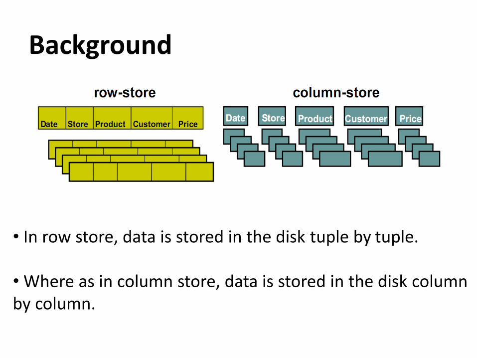
• In row store, data is stored in the disk tuple by tuple.

• Where as in column store, data is stored in the disk columnby column.

• Most of the queries does not process all the attributes of a particular relation.

• For example the query

Select c.name and c.address

From CUSTOMERS as c

Where c.region=Waterloo;

• Only process three attributes of the relation CUSTOMER. But the customer relation can have more than three attributes.

• Column-stores are more I/O efficient for read-only queries as they read, only those attributes which are accessed by a query.

Row Store Column Store

(+) Easy to add/modify a record (+) Only need to read in relevant data

(-) Might read in unnecessary data

(-) Tuple writes require multiple accesses

• So, column stores are suitable for read-mostly, read-intensive, large data repositories.

WHY COLUMN-STORES?

• Can be significantly faster than row stores for some applications– Fetch only required columns for a query– Better cache effects– Better compression (similar attribute values within a

column)

• But can be slower for other applications– OLTP with many row inserts, ..

• Long war between the column store and row store – This paper tries to give a balanced picture of advantages

and disadvantages, after adding/ subtracting a number of optimizations for each approach

Star Schema Benchmark (SSBM)

• SSBM is a data warehousing benchmark derived from TPC-H

• It consists of a single fact table LINE-ORDER • There are four dimension table.

– CUSTOMER – PART – SUPPLIER – DATE • LINEORDER table consists of 60,000,000 tuples• SSBM consists of thirteen queries divided into four

categories (or flights).

Row Oriented Execution

• Now the simplistic view about the difference in storage layout leads to the assumption that one can obtain the performance benefits of a column-store using a row-store by making some changes to the physical structure of the row store.

• These changes can be

– Vertically partitioning

– Using index-only plans

– Using materialized views

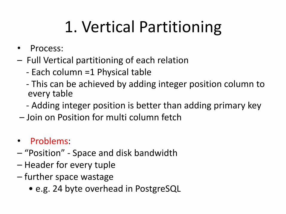
1. Vertical Partitioning• Process: – Full Vertical partitioning of each relation

- Each column =1 Physical table - This can be achieved by adding integer position column to every table - Adding integer position is better than adding primary key

– Join on Position for multi column fetch

• Problems: – “Position” - Space and disk bandwidth – Header for every tuple– further space wastage

• e.g. 24 byte overhead in PostgreSQL

• Each attribute is a two-column table: (values, position).

2. Index Only Plans

• Process:

– Add B+Tree index for every Table.column

– Plans never access the actual tuples on disk

– Headers are not stored, so per tuple overhead is less

• Problems:

– Separate indices may require full index scan, which is slower.

An optimization of Index only approach is to create indices with composite keys, where the secondary keys are from predicate-less columns

Eg: SELECT AVG(salary) FROM emp WHERE age > 40 – Composite index with an (age, salary) key helps.

– Slow Tuple Construction

• Unclustered B+Tree index for every column of everytable

3. Materialized Views

• Process:

– Create ‘optimal‘ set of MVs for given query workload

– Objective:

• Provide just the required data

• Avoid overheads

• Perform better

• Expected to perform better than other two approaches

• Problems:

– Practical only in limited situations

– Requires knowledge of query workloads in advance

• Select F.custID from

Facts as F where

F.price>20

Column Oriented Execution

• Different optimizations for improving performance of column oriented databases :

- Compression

- Late Materialization

- Block Iteration

- Invisible Joins

1. Compression

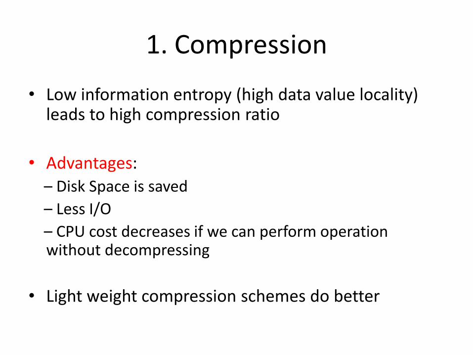
• Low information entropy (high data value locality) leads to high compression ratio

• Advantages:– Disk Space is saved

– Less I/O

– CPU cost decreases if we can perform operation without decompressing

• Light weight compression schemes do better

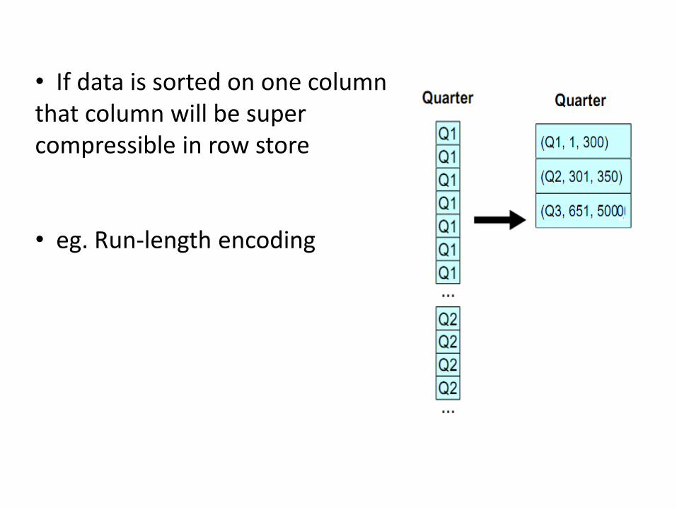
• If data is sorted on one column that column will be super compressible in row store

• eg. Run-length encoding

2. Late Materialization• Most query results entity-at-a-time not column-at-a-

time

• So at some point of time, multiple column must be combined

• One simple approach is to join the columns relevant for a particular query

• But further performance can be improve using late-materialization

• Delay Tuple Construction

• Might avoid constructing it altogether

• Intermediate position lists might need to be constructed

• Eg: SELECT R.a FROM R WHERE R.c = 5 AND R.b = 10

– Output of each predicate is a bit string

– Perform Bitwise AND

– Use final position list to extract R.a

• Advantages:

– Unnecessary construction of tuple is avoided

– Direct operation on compressed data

– Cache performance is improved (PAX)

3. Block Iteration

• Operators operate on blocks of values at once

• Iterate over blocks of values from same column

• Like batch processing

• If column is fixed width, it can be operated as an array

• Advantages: – Minimizes per-tuple overhead

– Exploits potential for parallelism

• Can be applied even in Row stores – IBM DB2 implements it

4. Invisible Joins

• Queries over data warehouses (particularly those modelled with star schema) often have following structure :

– Restrict the set of tuple in the fact table using selection predicates on dimension table

– Perform some aggregation on the restricted fact table

– Often grouping by other dimension table attribute

• For each selection predicate and for each aggregate grouping, a join between fact table and dimension table is required

• Find Total revenue from Asian customers who purchase a product suppliedby an Asian supplier between 1992 and 1997 grouped by nation of the customer, supplier and year of transaction .

• Traditional plan for this type of query is to pipeline join in order of predicate selectivity

• Alternate plan is late materialized join technique

• But both have disadvantages:

– Traditional plan lacks all the advantages described previously of late materialization

– In the late materialized join technique group by columns need to be extracted in out-of-position order

• Invisible join is a late materialized join but minimizes the values that need to be extracted out of order

• Invisible join

– Rewrites joins into predicates on the foreign key columns in the fact table

– These predicates are evaluated either by hash-lookup

– Or by between-predicate rewriting

Each predicate is applied to the appropriate dimension table to extract a list of dimension table keys that satisfy the predicate.

PHASE 1

Each hash table is used to extract the positions of recordsin the fact table that satisfy the corresponding predicate.

PHASE 2

The third phase uses the list of satisfying positions P in the fact table to get foreign key values and hence needed data values from the corresponding dimension table.

PHASE 3

• Between-Predicate rewriting

– Use of range predicates instead of hash lookup in phase1

– Useful if contiguous set of keys are valid after applying a predicate

– Dictionary encoding for key reassignment if not contiguous

– Query optimizer is not altered. Predicate is rewritten at runtime

Experiments

• Goal :

– Comparison of attempts to emulate a column store in a row-store with baseline performance of C-Store

– Is it possible for an unmodified row-store to obtain the benefits of column oriented design?

– Effect of different optimization techniques in column-store

Experimental Setup

• Environment :

– 2.8GHz Dual Core Pentium(R) workstation

– 3 GB RAM

– RHEL 5

– 4 disk array mapped as a single logical volume

– Reported numbers are average of several runs

– Warm buffer pool (30% improvement for both systems)

- Data read exceeds the size of buffer pool

C-store vs. Commercial Row Oriented DB

RS: Base System XRS (MV): System X with optimal collection of MVsCS: Base C-Store caseCS (Row--MV): Column store constructed from RS(MV) System X: Commercial row-oriented database

Results and Analysis

• From the graph we can see

– C-Store outperforms System X by a

--Factor of six in the base case

--Factor of three when System X uses materialized view

• However CS (Row-MV) perform worse than RS (MV)

– System X provides advance performance feature

– C-Store has multiple known performance bottleneck

--C-Store doesn't support partitioning, multithreading

Column store simulation in row store

• Partitioning improves the performance of row store if done on a predicate of the query

• Authors found that it improves the speed by a factor of two

• System X implements star join

• Optimizer will use bloom filters if it feels necessary

• Other configuration parameters

– 32 KB disk pages

– 1.5 GB maximum memory for sort joins, intermediate result

– 500 MB buffer pool

Different configurations of System X

Experimented with five different configurations:

1. Traditional row oriented representation with bitmap and bloom filter

2. Traditional (bitmap): Biased to use bitmaps; might be inferior sometimes

3. Vertical Partitioning: Each column is a relation

4. Index-Only: B+Tree on each column

5. Materialized Views: Optimal set of views for every query

T –Traditional,T(B) –Traditional(bitmap),MV – materialized views, VP – vertical partitioning,

AI –All indexes

• Better performance of traditional system is because ofpartitioning.

• Partitioning on orderdate

T –Traditional,T(B) –Traditional(bitmap),

MV – materialized views,

VP – vertical partitioning,

AI –All indexes

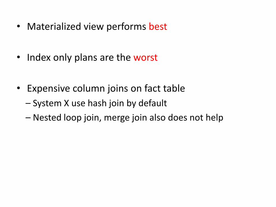
• Materialized view performs best

• Index only plans are the worst

• Expensive column joins on fact table

– System X use hash join by default

– Nested loop join, merge join also does not help

Column Store Performance

• Column Store perform better than the best case of row store (4.0sec Vs 10.2sec)

• Because column stores do not suffer from tupleoverhead and high column join costs.

Tuple Overheads and Joins

Row Store Column Store

Store the record-id explicitly Don’t explicitly store the record-id

Headers are stored with each column Headers are stored in separate columns

Use index-based merge join Use merge join

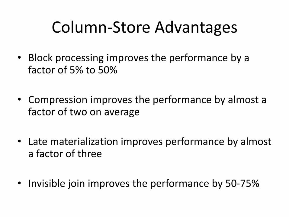
Column-Store Advantages

• Block processing improves the performance by a factor of 5% to 50%

• Compression improves the performance by almost a factor of two on average

• Late materialization improves performance by almost a factor of three

• Invisible join improves the performance by 50-75%

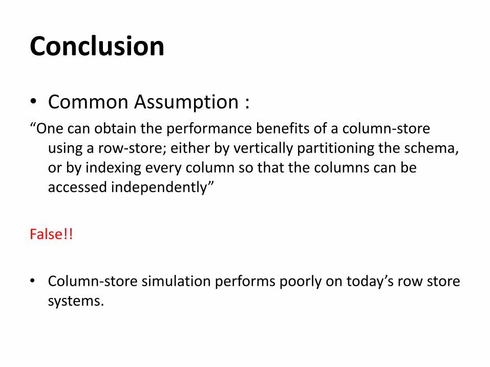
Conclusion

• Common Assumption : “One can obtain the performance benefits of a column-store

using a row-store; either by vertically partitioning the schema, or by indexing every column so that the columns can be accessed independently”

False!!

• Column-store simulation performs poorly on today’s row store systems.

• To simulate column store in row store, techniques like – Vertical partitioning

– Index only plan

do not yield good performance

• High per-tuple overheads, high tuple reconstruction costs are the reason

• Where as in column store

– Late materialization

– Compression

– Block iteration

– Invisible join are the reasons for good performance

Discussion

• In the future, where do you see this going? Column store simulation in row store or row store simulation in column store? Which will be more widely used?

• How do you think read/write locks for column store work?

• When to you use row, and when column ?