combinatorial models of creation{annihilation
TRANSCRIPT

Seminaire Lotharingien de Combinatoire 65 (2011), Article B65c
COMBINATORIAL MODELS OF CREATION–ANNIHILATION
PAWEL BLASIAK AND PHILIPPE FLAJOLET
Abstract. Quantum physics has revealed many interesting formal proper-
ties associated with the algebra of two operators, A and B, satisfying the
partial commutation relation AB −BA = 1. This study surveys the relation-ships between classical combinatorial structures and the reduction to normal
form of operator polynomials in such an algebra. The connection is achieved
through suitable labelled graphs, or “diagrams”, that are composed of ele-mentary “gates”. In this way, many normal form evaluations can be system-
atically obtained, thanks to models that involve set partitions, permutations,
increasing trees, as well as weighted lattice paths. Extensions to q-analogues,multivariate frameworks, and urn models are also briefly discussed.
Contents
1. Introduction 22. Diagrams, normal ordering, and enumeration 52.1. Gates, diagrams and labelling. 52.2. The equivalence principle. 72.3. Proof of the Equivalence Principle (Theorem 1). 92.4. Combinatorial enumeration. 143. Linear forms (X +D), involutions, and generalizations 153.1. The basic linear case (X +D). 153.2. Generalizations to (X +Dr) and (Xr +D). 174. The special quadratic form (XD), set partitions, and product forms 194.1. The form (XD) and set partitions. 194.2. The product form (X2D2). 234.3. Higher order forms (XrDr). 285. Quadratic forms (X2 +XD +D2), zigzags, and permutations 295.1. The circle form (X2 +D2) and zigzags. 295.2. The general quadratic form (αD2 + β X2 + γ XD). 316. Semilinear forms (φ(X)D) and increasing trees 346.1. The form (X2D) and increasing trees. 346.2. The general case (φ(X)D). 366.3. The form (φ(X)D + ρ(X)) and planted trees. 397. Binomial forms (Xa + Db), lattice path models, and continued
fractions 407.1. Normal ordering and lattice paths. 407.2. Fermat forms (Xr +Dr) and continued fractions. 437.3. The general binomial case (Xa +Db). 478. Related frameworks 488.1. Rook placements, lattice paths, and diagrams. 488.2. q−analogues and the difference operator. 519. Multivariate schemes. 5610. Perspectives 64

2 P. BLASIAK AND P. FLAJOLET
References 66Appendix A. Scherk’s dissertation of 1823 72
1. Introduction
The theme of our study is extremely simple. It consists in investigating someof the formal consequences of the partial commutation relation between two oper-ators A and B (belonging to some unspecified algebra of operators):
(1) [A,B] = 1.
Here [U, V ] := UV − V U is the Lie bracket and 1 represents the identity operator.The relation (1) will henceforth be called the creation–annihilation axiom. Indeed,in quantum physics1, it is satisfied by the annihilation and creation operators, a anda†, which are adjoint to each other and serve to decrease or increase the number ofphotons by 1: in this context, one should take A = a and B = a†.
From an algebraic standpoint, one thus considers the polynomial ring C〈A,B〉 innon-commuting indeterminates A,B, and makes systematic use of the reduction ofAB−BA−1 to 0. (Technically, this corresponds to taking the quotient C〈A,B〉/I,of the ring C〈A,B〉 of polynomials in non-commuting indeterminates by the two-sided ideal I generated by AB − BA − 1.) It is then possible to regard (1) as adirected rewrite rule
(2) AB −→ 1 +BA,
by which any non-commutative polynomial h in indeterminates A,B is completelyreduced to a unique normal form, N(h), where, in each monomial, all the occur-rences of B precede all the occurrences of A.
For instance, the chain
(3)ABABA −→ AB(1 +BA)A ≡ ABBAA+ABA
−→ ABBAA+A+BAA −→ BABAA+A+ 2BAA−→ BBAAA+ 3BAA+A
proves that N(ABABA) = B2A3 +3BA2 +A. (At each step, the pair AB involvedin a reduction has been underlined.) It is precisely this non-trivial rearrangementprocess, known in quantum physics as normal ordering, which we propose to ex-amine.
A particular realization of the commutation relation (1) is obtained by choosingsome sufficiently general space {f(x)} of smooth functions (typically, the class ofC∞(0, 1) of infinitely differentiable functions over the interval (0, 1), or the spaceC[x] of polynomials in indeterminate x), on which two operators, X and D aredefined:
(Xf)(x) = xf(x); (Df)(x) =d
dxf(x).
1The present paper deals with one or a finite number of pairs of such operators (known as
“modes”), a situation that is directly relevant to the “second quantization” of quantum theory,in particular, in quantum optics; see, for instance, Louisell’s book [89]. The case of a contin-uum of modes, which lies at the basis of quantum field theory and is associated with Feynmandiagrams [43, 44, 95, 132], is not touched upon here. The developments in our study require amodicum of combinatorial theory but no a priori knowledge of quantum physics.

COMBINATORIAL MODELS OF CREATION–ANNIHILATION 3
Then the creation–annihilation axiom is obviously satisfied by A = D and B =X: one recovers in this way the familiar Weyl relations [D,X] = 1 of abstractdifferential algebra [112, Ch. 1]. The interest of such a differential model of creation–annihilation is that it is “faithful”, meaning that any identity that holds in it(without any additional assumption regarding the space of functions) is true in allgenerality under (1). This differential view will prove central to our combinatorialdevelopments.
We henceforth adopt the more suggestive differential terminology, A 7→ D andB 7→ X. We shall concern ourselves here with the reduction to normal form of avariety of expressions such as
(4) (XD)n, (X2D)n, (D +X)n, (X2D2)n, (D2 +X2)n,
and many more. Observe that, by taking an exponential generating function, thecollection of all the reductions associated with a family (Hn)n≥0 is summarized bythe reduction of ezH.
Our starting point, to be developed in Section 2, is a combinatorial representa-tion of any normal-form monomial m = XrDs by a basic graph, called a “gate”.The reduction of a polynomial in operators D,X (for instance, any of (4)) canthen be regarded combinatorially as the process of building a whole collection oflabelled diagrams, which are those special graphs assembled from a fixed collectionof elementary gates (the ones arising from the monomials in (4)). From here, aswe shall see repeatedly, obtaining the coefficients in the normal form of an operatorexpression is equivalent to enumerating complex graphs built from a fixed collectionof gates. In other words, we are going to explore the following Equivalence Principle(see Theorem 1 below for a precise formulation):
Normal ordering(operator algebra)
⇐⇒ Diagram enumeration(combinatorics)
In so doing, we build on classical works in combinatorial analysis relative to the com-binatorics of differential operators; see, for instance, Joyal’s theory of species [74],its exposition in the book by Bergeron, Labelle and Leroux [7], or the recent bookby Flajolet and Sedgewick [51], whose notations we adopt.
The idea of using graphs to model creation–annihilation is not new. The mostcelebrated originator of the representation of physical processes by labelled graphsis R.P. Feynman, who used it as a convenient book-keeping tool for perturbativeexpansions of quantum electrodynamics [43, 44] and the whole idea is is neatly artic-ulated by Baez and Dolan in [3, pp. 46–49]. Seen under the interesting perspectiveof [3], what we propose to do is “decategorize” the abstract creation–annihilationtheory by providing concrete combinatorial models of this theory. Our standpointis however different in that we place a strong emphasis on connections with classicalcombinatorial structures and aim at developing exactly solvable models, hence ex-plicit formulae. With this in mind, we tread in the steps of earlier works of Blasiak,Duchamp, Horzela, Mendez, Penson, and Solomon [10, 11, 14, 15, 17, 19, 99] forwhich the present article can serve inter alia as a synthetic and systematic review.
Our purpose is to shed light on calculations developed within quantum physicsand do so by means of adapted combinatorial models. For instance, set partitions(with their associated Bell and Stirling numbers) naturally arise from diagramscorresponding to powers of XD, a fact largely known in combinatorics and finite

4 P. BLASIAK AND P. FLAJOLET
Hn Structure Generating function type
(X +D)n involutions ez2/2 §3
(XD)n set partitions eez−1 §4
(X2 +D2)n alternating cycles1√
cos(2z)§5.1
(XrD)n increasing trees exp
(1
(1− (r − 1)z)1/(r−1)− 1
)§6
(X2D)n permutations exp
(z
1− z
)§6.1
Figure 1. Some normal ordering problems relative to Hn, the corre-sponding combinatorial structures, a representative counting generatingfunction, and the relevant section in this article.
difference calculus, which is examined, under a quantum field angle, by Bender,Brody, and Meister in [5], and is further treated by Mendez, Blasiak, and Pensonin [99]. Also, by providing a complete permutation model, we explain and extendcalculations done by Mehta [96] that are relative to the normal ordering of
ezQ(X,D), where Q(X,D) = αD2 + βX2 + γXD
Finally, the combinatorial approach we advocate provides, in a number of cases,a transparent alternative to the Lie algebra approach exemplified by Wilcox [133].Figure 1 lists a representative set of operators discussed in this paper, together withthe underlying combinatorial structures and the corresponding generating functiontypes, as summarized in each case by a prototypical instance.
Plan of the paper. Section 2 presents the basic combinatorial model of gatesand diagrams, by which normal ordering is reduced to counting problems. It alsocontains a brief reminder of the symbolic approach to combinatorial enumerationvia generating functions (§2.4). We then consider the normal ordering problemrelative to hn in increasing order of complexity of the polynomial h. Section 3concerns the simplest case of linear forms in X,D, for which the natural model isseen to be that of (coloured) involutions. In Section 4, we proceed with the specialquadratic form (XD), which is tightly coupled with set partitions. The generalquadratic form in X,D treated in Section 5 leads to “zigzags”, which are structuresrelated to alternating permutations, and to local order patterns in (unconstrained)permutations. Section 6 shows that semilinear operators of the form (φ(X)D) arein general modeled by simple varieties of trees and forests. Section 7 momentarilydeparts from our main thread and introduces lattice path models: it presents adirect treatment of binomial forms, including the interesting “Fermat case” (Xr +Dr), which is conducive to continued fraction representations. Section 8 discussestwo frameworks that are closely related to diagrams: one is the rook placementmodel, for which a general scanning algorithm schema provides an alternative tothe methods of Section 7; the other is the planar embedding of diagrams, whichleads to a systematic approach to many q–analogues of combinatorial theory. Weconclude in Section 9 with a brief discussion of multivariate extensions of the gates-and-diagram model.

COMBINATORIAL MODELS OF CREATION–ANNIHILATION 5
The present paper contains few new results. Rather, it is an attempt at asynthetic presentation of the combinatorial approach to normal ordering problems,which has been the subject of an extensive literature in recent decades. Whatwe found striking, when preparing this paper, is the fact that most (perhaps all?)explicitly known expansions in this orbit of questions can be put in correspondencewith classical or semi-classical combinatorial models. As we hope to demonstrate,one of the interests of the combinatorial approach in this range of problems is tobring clarity into what should be explicit and what is not likely to be.
2. Diagrams, normal ordering, and enumeration
In this section, we associate with each polynomial in the operators X,D a finitecollection of elementary “gates” that are graphs with just one inner vertex, as in (5)below. We then define “diagrams” that are complex graphs built by assemblingelementary gates according to certain rules. (Our terminology is inspired by thatof digital circuits composed of elementary boolean gates.) A fundamental andeasy theorem (Theorem 1) then relates the normal ordering of the powers hn of apolynomial h to the enumeration of labelled diagrams of size n that can be builtout of the gates associated with h.
2.1. Gates, diagrams and labelling. We make use of the standard definitionsof graph theory, as found, for instance, in [33]. We however need to extend it some-what. Technically, our diagrams are directed multigraphs—edges are directed, mul-tiple edges between two vertices are allowed—that are further enriched by placingan ordering on the edges stemming from a vertex and similarly for edges leadinginto a vertex. (Put otherwise, we are considering graphs given together with anembedding into the plane.) We recall that the indegree and outdegree of a vertexare, respectively, the number of incoming and outgoing edges of that vertex. Inwhat follows, we freely make use of graphical representations to illustrate our basicnotions, while avoiding long formal developments; see Figure 2.
Definition 1. A gate of type (r, s) consists of a vertex, called the inner node, towhich is attached an ordered collection of r outgoing edges and an ordered collectionof s ingoing edges. The vertices, not the inner node, that have indegree 0 are calledthe inputs; the vertices, not the inner node, that have outdegree 0 are called theoutputs.
A gate thus comprises r+ s+ 1 nodes in total. The inner node is conventionallycoloured in black (•), whilst the input and output nodes are coloured in grey (NM)and white (M) respectively. For instance:
(5) gate of type (r, s) :
r outputs
s inputs.
In the graphical representation, edges are systematically (and implicitly) orientedfrom bottom to top; they are naturally ordered among themselves, conventionally,from left to right.

6 P. BLASIAK AND P. FLAJOLET
H :
δ :
21 6
83
4
9
7
5
10
Figure 2. Left: a collection H of two gates of type (2, 2) and (2, 1).Right: a labelled diagram δ on the basis H that comprises three com-
ponents.
Definition 2. A diagram is a directed multigraph, which is acyclic (i.e., has nodirected cycle) and is such that, for each vertex, an ordering has been fixed onits incoming and on its outgoing edges. In addition, there are a designated set ofinputs (vertices with indegree 0 and outdegree 1) and a designated set of outputs(vertices with indegree 1 and outdegree 0). The vertices that are neither inputs noroutputs are called inner nodes. The size of a diagram is the number of inner nodes2
it comprises.
The colouring convention of gates, as in (5), is extended to the representationof diagrams; see Figure 2 for an instance. Note that a diagram is not necessarilyconnected: it may be comprised of several (weakly connected) components. Clearly,a diagram specifies the collection of gates it is composed of.
Definition 3. Given a set H of gates, assimilated to a subset of Z≥0 × Z≥0, adiagram δ is said to have H as a basis if, for each outdegree–indegree pair (r, s) ofan inner node of δ, one has (r, s) ∈ H.
Finally, we need to introduce a crucial notion of labelling, which is consistentwith the standard one of combinatorial analysis [7, 51, 59, 122, 134], to which anadditional monotonicity constraint is adjoined.
Definition 4. A labelled diagram is comprised of an unlabelled diagram in thesense of Definition 2 together with an assignment of integer labels to inner nodesin such a way that: (i) all labels are distinct and they form an initial segment ofZ≥1; (ii) labels increase along any directed path.
Note that a labelled diagram can be interpreted as representing the completehistory of a particular incremental construction of an unlabelled diagram by suc-cessively “grafting” gates one after the other (Figure 3), following the order given
2In what follows, we shall discount from size outer nodes NM and M (which have size 0), andthen often use the term “vertex” and “inner node” (or simply “node”) interchangeably.

COMBINATORIAL MODELS OF CREATION–ANNIHILATION 7
δ : γ :
Figure 3. A particular grafting of a gate δ = XrDs (here, r = 3, s =2) on a diagram γ corresponding to a term XaDb (with a = 3, b = 4),in the case where two edges are matched (t = 2).
by the labels—this viewpoint will prove useful in Subsection 2.3. The enumerationof labelled diagrams corresponding to a fixed basis H of gates is a central aspect ofour approach to the creation–annihilation algebra3.
2.2. The equivalence principle. We propose to state a general form of the Equiv-alence Principle (Theorem 1 below), in which gates and diagrams can be weighted.Fix a field K, called the domain of weigths—it may be the field C of complex num-bers, in the case of numeric weights, or a field C(x, y, . . .) of rational functions informal variables x, y, . . ., in the case of symbolic weights. A weighting of a collectionH of gates is an assignment of a weight wr,s ∈ K to each gate of H; equivalently, afunction w : H −→ K. Such a weighting on gates induces a weighting on diagrams:the weight w(δ) of a diagram δ is defined to be the product of the weights of theindividual gates that the diagram is comprised of. Finally, the total weight4 of aclass D of diagrams is
∑δ∈D w(δ). With this convention, we state:
Theorem 1 (Equivalence Principle). Consider a polynomial h with normal form
(6) h :=∑
(r,s)∈H
wr,sXrDs.
Then the normal ordering of the power hn,
(7) N(hn) =∑n,a,b
cn,a,bXaDb,
is such that the coefficient cn,a,b coincides with the total weight of (monotonically)labelled diagrams that admit H as a basis weighted by w, have size n, and arecomprised of a outputs and b inputs.
3As pointed out to us by Ch. Brouder and G. Duchamp (October 2010), an early ancestorof the diagrams presented here is to be found in the 1965 book of Friedrichs [57] relative to
perturbation of spectra in Hilbert Space; see, especially, pages 55–56. We note also that thediagrams can be cast into the framework of [99] by a bijective correspondence “gates“↔ “bugs“
and “diagrams“↔ “colonies“.4Thus “total weight” extends the notion of “cardinality” or “number of elements” and deter-
mining total weights can be regarded as a (generalized) enumeration problem.

8 P. BLASIAK AND P. FLAJOLET
monomial XrDs ! gate of type (r, s)polynomial h in X,D ! weighted basis H of gateshn ! labelled diagrams of size n on Hezh ! all diagrams (exp. generating function)
(znXaDb) ! (size = n, #outputs = a, #inputs = b).
Figure 4. The correspondences between normal forms of algebraicexpressions in X,D, z (left) and combinatorial diagrams (right).
The proof is deferred until the next subsection. The interest of Theorem 1lies in the fact that it transforms an algebraic normal-ordering problem into acombinatorial enumeration problem, one that may be studied by the methods ofcombinatorial analysis. It is precisely our aim to explore aspects of this equivalenceand the derivation of explicit normal forms, based on combinatorial theory.
We note that Theorem 1 can be rephrased in terms of generating functions.First, by (7), the quantity N(hn) is the generating polynomial of labelled diagramswith X marking outputs, and D marking inputs: as in the case of gates, a diagramwith a outputs and b inputs corresponds to a term XaDb in the normal form.Introduce next the operator exponential
ezh :=∑n≥0
hnzn
n!,
which is a formal power series in z with coefficients in the polynomial ring C〈X,D〉and the corresponding normal form
N(ezh) =∑n≥0
N(hn)zn
n!.
Then, equation (7) expresses the fundamental identity
(8) N(ezh) =
∑n,a,b
cn,a,buavb
zn
n!
{u→ Xv → D
.
The sum on the right-hand side is nothing but the exponential generating function(EGF) of the total weight (number) of diagrams built on the weighted basis H,where z marks size, u marks the number of outputs, and v marks the number ofinputs. In writing such equalities, it is understood that all occurrences of X shouldbe systematically written5 to the left of all occurrences of D.
Theorem 1 thus expresses a general correspondence between the world of oper-ators and the realm of combinatorics, which is summarized in Figure 4.
5 Thus, one calculates generating functions of diagrams in the usual way, then, at the end,
one should group all occurrences of u before those of v, and finally perform the substitutionu → X, v → D. If G(z;u, v) is the generating function of diagrams, a notation often used byphysicists to indicate this process is
: G(z;X,D) :
which plainly represents a commutative image, with all Xs conventionally preceding all Ds, theninterpreted back as an operator in non-commuting X,D.
COMBINATORIAL MODELS OF CREATION–ANNIHILATION 9
2.3. Proof of the Equivalence Principle (Theorem 1). For the proof of The-orem 1, a basic observation is the identity
(9) (XrDs)(XaDb) =
s∑t=0
(s
t
)(a
t
)t!Xr+a−tDs+b−t.
Without loss of generality, it suffices to consider the case r = b = 0. Then, withthe interpretation Df(x) = d
dz f(x) and Xf(x) = xf(x), we find, by Leibniz’s rule,
(DsXa)f(x) ≡ Ds(xaf(x)) =
s∑t=0
(s
t
)(Dtxa)(Ds−tf(x))
=
s∑t=0
(s
t
)(a
t
)t!xa−t(Ds−tf(x)).
The last line implies (9), upon multiplying on the left by Xr and on the right by Db.Let now XaDb be a monomial that figures explicitly in N(hn) and let XrDs be
a monomial of h. The reduction to normal form of hn+1 (viewed as hn+1 = h ·hn) isobtained by applying the rule (9), then summing over all values (r, s) ∈ H. Assumenow, by induction that the identity (7) of Theorem 1 holds for a certain value of n,so that the coefficients of N(hn) count (with suitable weights) all diagrams of size n.The collection of legal diagrams of size n+ 1 is obtained by grafting in all possibleways a gate of the basis H on a diagram of size n. If this diagram δ has a outputsand b inputs and the gate γ is of type (r, s), then the number of ways that sucha grafting can be effected, when t outputs of δ are plugged into t inputs of γ isexactly
(10)
(s
t
)(a
t
)t!.
(The binomials count the choices of the t inputs of γ and the choices of the toutputs of δ that are matched; the factorial counts the possibilities of attachment.)Figure 3 displays a particular attachment of a gate of type (3, 2) to a connecteddiagram with 3 outputs and 4 inputs.
It is then observed, from a comparison of (9) and (10) that the multiplicitiesinduced either by a reduction of a left multiplication by XrDs or by adding a gateof type (r, s) are the same. Thus, the property that N(hn+1) is the generatingfunction of diagrams of size n+ 1 with X marking outputs and D marking inputsis established. The property trivially holds for N(h), ensuring the basis of theinduction. The proof of Theorem 1 is now complete.
Note 1. The combinatorics of derivatives and Wick’s Theorem. The usual rule of calculusDxn = nxn−1 has combinatorial content. For instance, D(x4) = 4x3 can be obtained as
D(xxxx) =6 xxxx+ x6 xxx+ xx6 xx+ xxx6 x,
corresponding to the formal rule: select in all possible ways an occurrence of the variable(x) and replace it by a neutral element (1). This lifts to arbitrary classes of combinatorialobjects as a general “pointing–erasing” operation [51, p. 201], which applies to “atoms”(basic components of size 1, such as letters of words or vertices of graphs) that composecombinatorial structures.
Equipped with this combinatorial interpretation of D, we can proceed to revisit thenormal form problem. As before X is the operator of multiplication by the variable x (i.e.,(Xf)(x) = xf(x), for an arbitrary function f(x)). Combinatorially, if f is regarded asrepresenting an arbitrary combinatorial class whose elements are made of x-atoms, then

10 P. BLASIAK AND P. FLAJOLET
Xf means adjoining—or “creating”— one new atom for each element of f . Consider nowthe normal form of an expression such as DX2. It can be obtained by working out whatDX2f is: first X2f adds two atoms; next, when D is applied, it must either pick upand erase one of these added x-atoms or hit and destroy an atom of f . In summary, theexternal D either “annihilates” one occurrence of a following X or it gets directly appliedto f itself. Pictorially,
DX2f = 6D 6XXf + 6DX 6Xf +DXXf = 2Xf +X2Df,
so that
N(DX2) = 2X +X2D.
Similar developments apply to arbitrary monomials in D and X, giving rise to what isknown in quantum physics as Wick’s Theorem and is usually expressed in terms of theannihilation a and creation a† operators. (Here, we can interpret a as D and a† as X.)
Proposition 1 (Wick’s Theorem). The normal form of a monomial in X,D equals thesum of all expressions obtained by removing in all possible ways an arbitrary number ofpairs D . . .X of annihilation (D) and creation (X) operators, where D precedes X, thenreorganizing the resulting monomials in such a way that all Xs precede all Ds.
Such a removal is called a contraction. An example of a normal form computation in thisframework (with : E : representing the commutative reorganization where all Xs precede
all Ds, as in footnote(5)) is as follows:
DXDDXD = : DXDDXD︸ ︷︷ ︸no pair removed
:
+ : 6D 6XDDXD+ 6DXDD 6XD+DX 6DD 6XD+DXD 6D 6XD︸ ︷︷ ︸1 pair removed
:
+ : 6D 6X 6DD 6XD+ 6D 6XD 6D 6XD︸ ︷︷ ︸2 pairs removed
:
= X2D4 + 4 XD3 + 2 D2.
(From here, the proof of Wick’s Theorem is immediate: it suffices to proceed by inductionon the length of the monomial to be reduced, distinguishing the two cases N(Xw) andN(Dw), where w in an arbitrary monomial in X,D.)
The procedure that underlies Wick’s Theorem may involve a large number of steps, asit amounts to enumerating all possible sets of contractions. The computational complexityis thus exponential in the worst case. By contrast, the combinatorial approach based ondiagrams provides a graphical means to track down patterns in the diversity of Wick’scontractions, which can then be effectively used to achieve a reduction in computationalcomplexity and, in several cases, lead to closed-form solutions.
Next, we can interpret gates in the same vein: Ds corresponds to selecting a sequenceof s distinct atoms and replacing each of them by the neutral element, whereas Xr meansadding r new atoms. A derivative (D) then “hooks” on atoms (X) or it “jumps” to theright. A particular labelled diagram composed of gates (γ1, . . . , γn), with γj associatedwith XrjDsj , then corresponds to a particular expansion of
(XrnDsn) · · · (Xr2Ds2)(Xr1Ds1).
Identities such as (9) then receive a natural interpretation and the construction of diagramscan be entirely developed in this way from first principles—this approach will be revisitedin Section 8, when we discuss the q-difference operator ∆. . . . . . . . . . . . . . . . . . . . . . . . . . . . �

COMBINATORIAL MODELS OF CREATION–ANNIHILATION 11
1
43
5
2
5
23
4
1
Figure 5. A diagram (left) and its dual (right).
Note 2. Duality. There is an easy but important duality in reductions to normal forms.For noncommutative expressions in the two variables X,D, define an antimorphism ϕ bythe rules
(11) ϕ(X) = D, ϕ(D) = X, ϕ(U · V ) = ϕ(V ) · ϕ(U),
together with an extension to polynomials by linearity. Thus, for a monomial m, its imageϕ(m) is obtained by exchanging the roles of X and D as well as reading letters backwards.It is then observed that the basic quantity DX − XD − 1 is invariant under ϕ. As aconsequence, any identity U = V (modulo DX − XD = 1) over terms U,V in X,Dimmediately implies a dual identity ϕ(U) = ϕ(V).
This duality has a natural graph interpretation. Define the dual graph Γ by revertingthe arrows in Γ , relabeling the vertices • in reverse order (i.e., 1, 2, ..., n−1, n are changedinto n, n− 1, ..., 2, 1 respectively). The result is again a legitimate graph. See Figure 5 forillustration. Clearly, the dual graph is made of a basis of gates that is dual to the one ofthe original graph.
A consequence of the foregoing considerations is that the normal forms of hn and ofϕ(h)n involve the same coefficients, with the coefficient of XaDb in N(hn) being identicalto that of XbDa in N(ϕ(h)n). In this way, for instance, the normal forms we developbelow for (X2D)n immediately translate to the case of (XD2)n. (In physical contexts,duality is often associated with hermitian conjugacy; see Mikhailov’s article [101, §3] forseveral examples). . . . . . . . . . . . . . . . . . . . . . . . . . . . . . . . . . . . . . . . . . . . . . . . . . . . . . . . . . . . . . . . . . . �
Note 3. The combinatorics of Taylor’s formula. Here is a basic illustration of thecombinatorics of derivatives. It is well known, from several areas of analysis and thecalculus of finite differences6, that the exponential of a derivative plays the role of atranslation operator—also known as “shift”. Specifically, with the notations of Note 1, weconsider the operator
(12) Ty := eyD.
Symbolically, we have, corresponding to Taylor’s formula:
(13) Ty · f(x) =∑n≥0
yn
n!Dnf(x) =
∑n≥0
yn
n!f (n)(x) = f(x+ y).
6See, e.g., the treatises of Jordan [70, pp. 13–14] and Milne-Thomson [102, p. 33]. The interestof this symbolic view is inter alia to lead to an immediate proof of (a form of) the Euler–Maclaurin
summation formula by a computation of (eyD − 1)−1; cf [102, p. 260].

12 P. BLASIAK AND P. FLAJOLET
It is piquant to note that the formula admits a transparent combinatorial interpreta-tion, in view of Note 1. Think of f(x) as being the generating function of a class F ofcombinatorial objects, themselves composed of atoms represented by x:
f(x) =∑φ∈F
x|φ|.
The application of the operator 1n!Dn means: “select in all possible ways an unordered
collection of n atoms in each element of F and replace these by neutral atoms”. Theapplication of 1
n!ynDn then translates as follows: “select in all possible ways a collection
of n atoms of type x in each elements of F and replace these by y-atoms”. The exponentialeyD then corresponds to choosing an arbitrary number of x’s and replacing them by y’s,the outcome being exactly the bivariate generating function f(x + y). Thus, seen fromcombinatorics, Taylor’s formula
f(x+ y) =∑n≥0
yn
n!f (n)(x)
simply expresses the decomposition of a bicolouring process according to the number ofatoms whose colour is changed. Figuratively:
Bicolourx,y [F ] ≡∞⋃n=0
“change n occurrences of x into y in elements of F(x)”.
(This exercise appears, for instance, explicitly as Note III.31 in [51, p. 201].) . . . . . . . . �
Note 4. Normal forms and PDEs. The reduction of powers of differential operators tonormal form is of interest in the analysis of certain types of partial differential equations(PDEs). Consider the initial value problem, also known as “Cauchy problem”,
(14)
∂
∂tF (x, t) = ΓF (x, t), with Γ ∈ C[x, ∂], ∂ ≡ ∂x = ∂
∂x
F (x, 0) = f(x),
where Γ is a differential operator, which is a polynomial in x and ∂x. The solution isdetermined by the initial data f(x) at time t = 0. An equation of this sort is sometimesreferred to as an evolution equation, with the specific choice of the linear differentialoperator Γ serving to model various physical contexts. Classical examples, in the one-dimensional case, are the heat equation,
(15)∂F
∂t=∂2F
∂x2,
and the Schrodinger equation with time-independent potential V ≡ V (x):
(16) i~∂F∂t
= − ~2
2m
∂2F
∂x2+ V (x)F.
With the notations of (14), introduce the Ansatz
(17) F = etΓ f,
where the operator exponential is classically defined as
(18) etΓ :=
∞∑n=0
tn
n!Γn.
Proceeding formally, we verify that
(19)∂F
∂t=
(∂
∂tetΓ)f = ΓetΓ f = ΓF,

COMBINATORIAL MODELS OF CREATION–ANNIHILATION 13
while, by construction, F reduces to f at t = 0. (Analytically, sound uses of such operatorexponentials can be based on the theory of operator semigroups; see, for instance, thebook by Engel and Nagel [41], and especially its Chapter 6, for an accessible discussion.)
If now the normal form of the powers Γn can somehow be regarded as known,
etΓ =
∞∑n=0
tnn!An, with An =
∑α,β
a(n)α,βx
α∂β ,
then, a formal solution of the evolution equation (14) is
(20) F (x, t) =
∞∑n=0
tn
n!
∑α,β
a(n)α,βx
α∂βf.
It is naturally a nontrivial matter to make analytic sense of (20), which often proves tobe a divergent expansion, but the formal solution (20) should at least provide valuableclues as to the kind of special function involved in the analytic solution of the evolutionequation (14). . . . . . . . . . . . . . . . . . . . . . . . . . . . . . . . . . . . . . . . . . . . . . . . . . . . . . . . . . . . . . . . . . . . . . . . �
Note 5. The heat equation. To illustrate the usefulness of operator calculus, we brieflyshow how to rederive7 formally the solution of the heat equation (15) in the present per-spective. In accordance with the Ansatz (17), one should consider the operator exponential
et∂2
.We choose8 to examine the effect of the exponential-of-the-Laplacian et∂
2
on the col-lection of base functions {eiωx}, so that
et∂2
· eiωx =∑n≥0
tn
n!
((iω)2neiωx
)= e−tω
2
eiωx.
Then, if f(x) is a Fourier integral,
f(x) =
∫ +∞
−∞e−iωxφ(x) dω,
Equation (20) yields by linearity the formal solution
F (x, t) =
∫ +∞
−∞e−iωx
(e−tω
2
φ(ω))dω.
The function F ( · , t) thus appears as the Fourier transform of the product of the two
functions e−tω2
and φ(ω). This, by well known properties of the Fourier transform, whichexchanges convolutions and ordinary product, leads (formally still) to the celebrated “heatkernel” solution
(21) F (x, t) =1√4πt
∫ +∞
−∞exp
(− (x− y)2
4t
)f(y) dy.
In this particular case of the heat equation, the normal form problem relative to (∂2)n
is trivial. Nonetheless, the derivation above demonstrates the type of usage of operatorexponentials, once these can be made sufficiently “explicit”. It is one of our goals todevelop a combinatorial toolbox for the simplification of such exponentials, which couldthen serve as a preamble to the analysis of more complicated types of PDEs. . . . . . . . . �
7What follows is extremely classical material (see, e.g., [38, pp. 107–109]), only slightly rear-ranged to suit our needs.
8This choice actually corresponds to an eigenfunction expansion in disguise. For instance, ifΓ has known eigenvalues {λ} with eigenfunctions {v(x)}, then etΓ v(x) = etλv(x), from whichsolutions can be composed by linearity.

14 P. BLASIAK AND P. FLAJOLET
2.4. Combinatorial enumeration. Throughout this paper, we appeal to generalmethods of combinatorial analysis relative to the enumeration of labelled objectsand extensively base our discussion on the standard conventions of the book An-alytic Combinatorics [51, Ch. 2]. If C is a combinatorial class formed of labelledobjects (typically, diagrams), we systematically let Cn be the subclass of objects ofsize n, with Cn the corresponding cardinality. The exponential generating function(EGF) of the class is
C(z) :=∑n≥0
Cnzn
n!=∑c∈C
z|c|
|c|!.
What we want to do is construct complex combinatorial classes from simplerones. The initial classes include the atomic class Z, which comprises a singleelement of size 1 and has EGF z, as well as the neutral class E , which consists of asingle element of size 0 and has EGF 1
Disjoint unions, henceforth written plainly as ‘+’, clearly correspond to sums ofEGFs:
(22) C = A+ B =⇒ C(z) = A(z) +B(z).
The labelled product C = A ? B of two labelled classes is obtained by taking allthe ordered pairs (α, β), with α ∈ A and β ∈ B, then relabelling them in allorder-consistent ways so as to obtain a well-labelled pair (α′, β′). We then have thecorrespondence
(23) C = A ? B =⇒ C(z) = A(z) ·B(z).
It is then possible to form the class of all (labelled) sequences (‘Seq’), sets (‘Set’),and cycles (‘Cyc’) with components in A, the corresponding EGFs being given bythe following dictionary:
(24)
C = Seq(A) =⇒ C(z) =
1
1− C(z)C = Set(A) =⇒ C(z) = exp(C(z))
C = Cyc(A) =⇒ C(z) = log1
1− C(z).
These basic constructions suffice to transcribe the normal form problem in simplercases such as (X +D) in Section 3 and (XD) in Section 4.
Finally, we shall need the modified “boxed product” construction, C = (A2 ? B),which corresponds to the subset of ordered pairs (α, β) ∈ (A ? B), such that thesmallest label is constrained to belong to the α component; see Greene’s thesis [62],as well as the accounts in [7, Ch. 7] and [51, §II.6.3]. The translation rule fromconstructions to EGFs is
(25) C = (A2 ? B) , =⇒ C(z) =
∫ z
0
(d
dtA(t)
)·B(t) dt.
This covers in particular the min-rooting operation, which attaches an externalatom to a B–structure and assigns to it the smallest label: the construction issimply (Z2 ?B) and it corresponds to an integration operator
∫ z0B(t) dt. The same
translation applies to the dual boxed product C = (A� ? B), where it is now thelargest label that is constrained to belong to the A-component. We shall makemuch use of these constructions, which correspond to a decomposition according to

COMBINATORIAL MODELS OF CREATION–ANNIHILATION 15
1 2 3 85
9
4
7
6
Figure 6. A particular (X +D)–diagram.
the first or last gate of a diagram: they are used typically in Section 5, relative to(X2 +D2), and Section 6, relative to (X2D).
All the rules above extend to multivariate generating functions: these containextra parameters, which can keep track of various additive characteristics of struc-tures [51, Ch. III].
In the next sections, we are precisely going to make use of the dictionary formedby (22), (23), (24), and (25) in order to enumerate various classes of diagramsassociated (via Theorem 1) with the normal ordering of terms in the operators X,D.
3. Linear forms (X +D), involutions, and generalizations
This section is dedicated to the normal ordering of expressions of the form(a(X) + D)n and (a(D) + X)n, with a( · ) a polynomial, starting with the eas-ier case (X + D)n. Thus, the schema is that of a base form in X and D, whichis linear in at least one of the operators X,D. The combinatorial models turn outto be special coloured permutations (involutions and generalizations), for which theintroduction of diagrams easily leads to fully explicit forms.
3.1. The basic linear case (X + D). Linear forms in the operators X and D,namely, operators of the form
Γ = αX + βD,
can serve to illustrate the usefulness of diagrams with minimal apparatus. In ac-cordance with the developments of Section 2, we are talking here of diagrams basedon two types of gates: a gate X has no input and one output; a gate D has oneinput and no output:
.
By inspection of all the possible ways of assembling gates, it is immediately seenthat a diagram must be comprised of three types of components: isolated X–gates,isolated D–gates, and pairs DX, where a D is hooked to an earlier arrived X. Inthe labelled case, the isolated X and D may receive arbitrary labels, while the“saturated” DX pairs are only constrained by the fact that the label of the X issmaller than the label of the D; see Figure 6.

16 P. BLASIAK AND P. FLAJOLET
Combinatorially, the class of all diagrams is thus specified by
G = Set(αZ + βZ + αβ Set2(Z)),
when the multiplicative weights α, β are taken into account. Here, the Set2 con-struction9 describes an unordered pair of two labels whose arrangement is imma-terial: the smaller label is necessarily attached to an X-gate, the larger one toa D-gate; see Figure 6. The generating function of all weighted diagrams is accord-ingly
(26) G(z) = e(α+β)z+αβz2/2.
An equivalent way of phrasing this result is as an equality,
(27) N(ez(αX+βD)
)= eαβz
2/2 · eαzX · eβzD,
where the right-hand side is to be interpreted as a standard expansion in the com-muting indeterminates X,D. A straight expansion then yields an explicit formof (27), ∑
k,`,m≥0
z2k
2k k!(αβ)k
z`
`!α`X` z
m
m!βmDm,
which, after collection of the coefficient of zn, can be summarized as follows10.
Proposition 2. The normal form of (αX + βD)n satisfies
N ((αX + βD)n) =∑`,m
I(n)`,mX
`Dm,
where, for n− `−m odd, the coefficients I(n)`,m are 0, while, for n− `−m even, they
satisfy
I(n)`,m =
n!
2(n−`−m)/2((n− `−m)/2)! `!m!α(n+`−m)/2β(n+`+m)/2.
In combinatorics, a permutation σ containing only cycles of sizes 1 and 2 isknown as an involution (it satisfies σ2 = 1). The specification and exponentialgenerating functions are accordingly
I = Set(Z + Cyc2(Z)), I(z) = ez+z2/2;
see, e.g., [51, p. 122]. The numbers I(n)`,m therefore enumerate coloured involutions,
where singleton cycles can receive any one of two colours (corresponding either toan X or a D). In other words: the natural combinatorial model for the normalordering of (X +D)n is that of (bicoloured) involutions.
The classical result expressed by Proposition 2 is usually derived in the contextof Lie groups by means of the Baker–Campbell–Hausdorff formula [58, 64], since,in this case, nested Lie brackets of higher order vanish. Indeed, it is known in thistheory that, if the commutator C = [A,B] commutes with both A and B, one hasthe general identity11 (see [58, p. 463] and [64, p. 64]):
ez(A+B) = ezA · e[B,A]z2/2 · ezB .9In this particular case, a Cyc2 construction can equivalently be used, given the obvious
combinatorial isomorphism Set2(Z) ∼= Cyc2(Z).10Proposition 2 is a classical result: it is for instance derived by means of operator calculus
methods in Wilcox’s paper [133, Eq. (10.43)], published in 1967.11Formulae of this sort are sometimes known as “disentanglement formulae” [29].

COMBINATORIAL MODELS OF CREATION–ANNIHILATION 17
Note 6. Solution of a special PDE by normal ordering of (X+D)n. The partial differentialequation of interest is
(28)∂F
∂t=∂F
∂x+ xF,
with initial value condition F (x, 0) = f(x). This is of the form considered when discussingoperator exponentials in Note 4, p. 12, here with Γ = (X + D). The operator solutionetΓ f , under the normal ordering provided by Equation (27) above, becomes
etΓ f = et2/2 · etx · etD f.
We know (from the earlier Note 3, p. 11) that the exponential of a derivative is a shift,etD f(x) = f(x+ t), so that the solution to (28) is the fully explicit
(29) F (x, t) = et2/2+xtf(x+ t),
whose validity is easily checked directly.No claim is made that the PDE (28) is hard to solve, and, indeed, it succumbs easily
to the method of characteristics, which is generally applicable to linear and quasilinearPDEs [124, §1.15]. It is nonetheless instructive to observe the way the reduction to normalordering (with the right factor etD) could automatically put us on the tracks of a generalsolution. . . . . . . . . . . . . . . . . . . . . . . . . . . . . . . . . . . . . . . . . . . . . . . . . . . . . . . . . . . . . . . . . . . . . . . . . . . . . �
3.2. Generalizations to (X + Dr) and (Xr + D). We next examine the caseof the operator (X + D2). According to the main theorem, one should considerdiagrams built out of two types of gates: D2–gates have two inputs and no output;X–gates have, as usual, one output and no input:
.
It is then easily realized that the only possibilities for connected diagrams are givenby the following list:
(30) .
For instance, D2X2 represents a connected component that is “saturated”, in thesense that the two inputs of a D2–gate are connected to the (earlier arrived) outputsof two X–gates; similarly, D2X2 depicts a component, for which the output of anX–gate is plugged into the first input of a D2–gate, while the second input remainsfree; and so on.
We can then look at the balance of inputs and outputs corresponding to each ofthe gates of the list (30). For instance, a D2X2 component has one input gate (adangling D) and no output, so that it is equivalent to a D, in terms of the balance

18 P. BLASIAK AND P. FLAJOLET
between number of inputs and number of outputs. Proceeding systematically, wedetermine the following table for all the possible types of connected components:
(31)type : D2 X D22X D2X2 D2X2
size : 1 1 2 2 3balance : D2 X D D 1.
Next, we should examine the number of ways of placing labels on connectedcomponents. In the case of a D22X or D2X2, the size equals 2, but the D2–gate is necessarily associated with the largest label; thus, any such component is aSet2(Z), itself combinatorially equivalent to a Cyc2(Z). In the case of a saturatedcomponent D2X2, two possible orderings are to be considered, since the first inputof D2 is associated with either the earlier arrived X or with the later X; in thiscase, the component turns out to be equivalent to a Cyc3(Z). Thus, using now,as standard commuting formal variables, u to mark components with a danglingoutput (X) and v to mark components with a dangling input (D), we have, for thevarious components, the specifications:
(32)type : D2 X D22X D2X2 D2X2
specification : v2Z uZ vCyc2(Z) vCyc2(Z) Cyc3(Z).
There results that the class of all diagrams is described by
G = Set(v2Z + uZ + vCyc2(Z) + vCyc2(Z) + Cyc3(Z)
),
with corresponding EGF
(33) G(z;u, v) = exp(v2z + uz + vz2/2 + vz2/2 + z3/3).
In other words, the model is now that of (multicoloured) permutations, all of whosecycles are of length at most three, where, in addition, singletons and doubletons canbe of any of two colours.
The very same reasoning applies to the normal ordering of (X2 +D)n. The dia-grams are isomorphic to the earlier ones, with inputs and outputs being exchangedand time being reversed. That is, the roles of X and D in (33) are simply to beexchanged—this is a special case of the general duality discussed in Note 2, p. 11.In summary:
Proposition 3. The normal orderings corresponding to the base operators (D2+X)and (X2 +D) satisfy
(34)
N(ez(D
2+X))
= ez3/3+zX · ez
2D+zD2
N(ez(X
2+D))
= ez3/3+z2X+zX2
· ezD .
Finally, the explicit normal forms associated with (D + a(X)) and (X + a(D)),for a( · ) a polynomial, are accessible via a combinatorial calculus that suitablyextends (31) and (32): the combinatorial model now involves permutations withcycles of length at most r. We leave it as an exercise to the reader to work outdetails and state12:
12Mikhailov [100] has a simple proof based on operator algebra in [100], and he refers to earlierworks of Witschel (1975) and Yamazaki (1952).

COMBINATORIAL MODELS OF CREATION–ANNIHILATION 19
Proposition 4. The normal ordering corresponding to the base operators (a(D) +X) and (a(X) +D) are given by
(35)
N(ez(a(D)+X)
)= ezX · exp
(∫ z
0
a(v + w) dw
)∣∣∣∣v 7→D
N(ez(a(X)+D)
)= exp
(∫ z
0
a(X + w) dw
)∣∣∣∣u7→X
· ezD.
In the pure binomial case of (Dr + X) and (Xr + D), the normal forms furthersimplify13 as N
(ez(D
r+X))
= ezX · exp(
1r+1
[(D + z)r+1 −Dr+1
])N(ez(X
r+D))
= exp(
1r+1
[(X + z)r+1 −Xr+1
])· ezD,
which gives back (27) and (34), when m = 1, 2.
Note 7. Another PDE. The usual consequences for PDEs also hold, with the furthersimplification that etD is a shift and that, for the quadratic case at least, the exponentialof the Laplacian can be made explicit in the Fourier basis of complex exponentials. Forinstance, the general PDE schema
∂F
∂t=∂F
∂x+ a(x)F,
admits the solution
F (x, t) = eQ(x,t)f(x+ t), Q(x, t) :=
∫ t
0
a(x+ w) dw.
In particular, a(x) = x2 corresponds to Q(x, t) = t3/3 + tx2 + t2x. . . . . . . . . . . . . . . . . . . . �
4. The special quadratic form (XD), set partitions, and product forms
This section is dedicated to the normal ordering of the powers (XD)n, a problemwhich has been recognized for a long time to be tightly coupled to set partitions andStirling numbers of the second kind. In Appendix A, we summarize the main resultscontained in the rather remarkable thesis memoir of Heinrich Scherk, defendedin 1823: the reduction of (XD)n figures there explicitly! We also consider, inthis section, the related quadratic form XD+ g(X +D). Finally, we show that thecombinatorial approach advocated here extends rather easily to powers of operatorssuch as X2D2, X3D3, and so on, which relates to several combinatorial enumerationproblems of independent interest.
4.1. The form (XD) and set partitions. By the general isomorphism theorem,the operator (XD) corresponds to a gate with one input and one output:
With these, we can form chains where the input of an XD–gate is connected tothe output of a previously arrived XD–gate. When time stamps are put on thevertices of the gates, a connected component becomes an increasing linear graph
13These formulae have also been found independently by Karol Penson (unpublished, 2004).

20 P. BLASIAK AND P. FLAJOLET
4
3
6
10
5 7
8
2
11
9
1
Figure 7. A particular diagram associated with (XD).
(see, e.g., [51, p. 99]), in the sense that vertices are linearly arranged and labelled inincreasing order, with the additional condition that size needs to be at least one: seeFigure 7. Note that edges between adjacent elements in a connected component areredundant and hence each chain can be represented by the nonempty set of labels.Here is a particular representation:
1 2 3 5 7
8
11
4
6
10
9
.
Under this form one recognizes the classical structure of set partitions, where apartition of a set is a subdivision of the elements of the set into indistinguishablenon-empty classes, also known as “blocks” [25, 51, 61]. (Here the components havebeen presented in increasing order of their leading elements.)
Components can be equivalently regarded as non-empty unordered collectionsof labels (non-empty “urns” in the terminology of [51, p. 99]); that is, they arespecified by K = Set≥1(Z). An arbitrary graph built out of XD–gates is then anunordered collection of such components, so that the corresponding class is Set(K).With z marking the size of a graph (its number of gates, equivalently, vertices) and umarking the number of connected components (here equal to the number of inputsand to the the number of outputs), we thus have for diagrams the specification
G = Set (uSet≥1(Z)) ,
hence the corresponding generating function
(36) G(z, u) = eu(ez−1).
COMBINATORIAL MODELS OF CREATION–ANNIHILATION 21
The generating functions solve the corresponding enumeration problems. By anexpansion of (36) taken at u = 1, the total number $n of partitions of a set ofcardinality n satisfies the “Dobinski relation”
(37) $n = n![zn]eez−1 = e−1
∑`≥0
`n
`!,
a quantity known in combinatorics as a Bell number [25]. The number of partitionsof n elements into k classes is the Stirling number of the second kind, nowadaysusually denoted by
{nk
}, whose value is [25, 51, 61]
(38)
{n
k
}= n![znuk]eu(e
z−1) =n!
kk =
1
k!
n∑j=0
(k
j
)(−1)k−jjn,
as can be immediately verified from a series expansion of (37).Back to the normal ordering problem, each connected component of a diagram,
i.e., each chain of XD–gates, has one input and one output, so that the balance of asingle component is of the form XD, the balance of k components being accordinglyXkDk. We then have:
Proposition 5. The normal ordering associated with ez(XD) involves the Stirlingpartition numbers:
(39)
N(ez(XD)
)= eu(e
z−1)∣∣∣〈uk 7→XkDk〉
=∑n≥0
zn
n!
[∑k
{n
k
}XkDk
]=
∑k≥0
1
k!(ez − 1)
kXkDk.
Note 8. Yet another PDE. Proceeding as before, we obtain from (39), that the PDE
∂F
∂t= x
∂F
∂x
with initial condition F (x, 0) = f(x) possesses the solution
F (t, x) =∑k≥0
(et − 1)kXkDk
k!f(x) = f(x(et − 1) + x) = f(xet),
whose a posteriori verification is immediate. . . . . . . . . . . . . . . . . . . . . . . . . . . . . . . . . . . . . . . . . �
Note 9. History. The origin of the Stirlng partition numbers{nk
}and their cognates, the
Sirling cycle numbers[np
], lies in eighteenth century calculus. The classical way of defining
them is as the coefficients expressing, in the polynomial algebra C[x], the change of basisbetween the canonical basis xn and the factorial basis xn ≡ x(x− 1) · · · (x− n+ 1) or itstrivial variant xn = x(x+ 1) · · · (x+ n− 1). Indeed, one has [61, pp. 248–249]:
(40) xn =∑k
{n
k
}xk, xn =
∑k
[n
k
]xk .
(In a different circle of ideas, Stirling numbers are known to probabilists as a way ofrelating factorial moments and standard power moments [31, p. 47].) Upon examiningthe effect on coefficients of power series, it is then seen that Stirling coefficients serve toexpress the connection between powers (x∂x)n and standard derivatives, via xk∂kx , whichis exactly what we derived by elementary combinatorics in (39). An equivalent operator

22 P. BLASIAK AND P. FLAJOLET
1 13
7
5
21
14
2 12
17
8
20
10 3
16
11
19
4 9
6
15
18
Figure 8. A sample diagram associated with (XD + g(X +D)).
formulation appears as an exercise14 in Comtet’s book [25, Ex. 2, p. 220]. (Some of theseproperties were already familiar to Scherk in 1823; cf Appendix A, p. 72.)
In the context of quantum physics, the combinatorial connections between the normalordering of (a†a)n and Stirling numbers have been recognized early: see, for instance, thepapers of Wilcox [133, p. 978], for an algebraic perspective, and especially Katriel [77], forthe combinatorial connection. (See also references therein to earlier works by Schwingerand others.) This thread has given rise to a large body of subsequent literature. Inparticular, Bender, Brody, and Meister explicitly discuss Bell numbers in the context ofdiagrams in [5], although their approach differs substantially from ours, as they focus on
interpretations of the schema eφ(D)eξ(X). The relations between set partitions, diagramsand Stirling numbers are used as a lead example by Baez and Dolan [3] to illustrate theprocess of “decategorifying” (!) the creation–annihilation theory. We examine below, inSubsection 4.2, further interesting extensions of the combinatorial approach that are dueto Blasiak et al. . . . . . . . . . . . . . . . . . . . . . . . . . . . . . . . . . . . . . . . . . . . . . . . . . . . . . . . . . . . . . . . . . . . . . �
Note 10. Normal forms relative to (XD+g(X+D)). We briefly discuss this case, whichis treated by Wilcox [133] and Louisell [89] by means of operator calculus, as it illustratesthe versatility of the combinatorial method. The gates are now of the three types X, Dand XD:
The connected components are similar to those relative to (XD), with, in addition, thepossibility that a line graph can be “capped” with a D, or “cupped” with an X, or bothcapped and cupped; they are consequently of four possible types. Hence, one can writedirectly the specification of graphs as
G = Set((uv + ug + vg) Set≥1(Z) + g2 Set≥2(Z)
),
where u and v mark inputs and outputs, respectively. The corresponding multivariateEGF is then
G(z;u, v) = e(x+g)(y+g)(ez−1)e−g2z.
(This case prefigures the planted-tree construction of Subsection 6.3, p. 39.) . . . . . . . . . �
14This interesting exercise also contains the reduction of (Xa+1D)n and its connection with
{(1−at)1/a− 1} [with the minor typo of a missing exponent of n], which we shall encounter laterin Section 6; see also Riordan [109, §6.6] for related operational calculus derivations.

COMBINATORIAL MODELS OF CREATION–ANNIHILATION 23
3
1 2
5
4
6
1
2
3
4
5
6
1’ 2’ 3’ 4’ 5’ 6’
7
7
Figure 9. The scaffolding representation of an X2D2 graph (and theinduced canonical labelling of lines).
4.2. The product form (X2D2). This subsection and the next one serve to revisitthe combinatorial works of Blasiak, Horzela, Penson, Solomon, and coauthors [10,15, 18, 19, 99]. See also Schork’s synthetic study [114], which furthermore includessome q-analogues. To avoid cumbersome notations, we start with a discussion ofthe operator X2D2. What is at stake is understanding the structure of reductionssuch as
(41)
(X2D2) = X2D2
(X2D2)2 = 2X2D2 + 4X3D3 +X4D2
(X2D2)3 = 4X2D2 + 32X3D3 + 38X4D4 + 12X5D5 +X6D6,
where the sums of the coefficients form a sequence $2,2n , which starts as
(42) ($2,2n ) = 1, 7, 87, 1657, 43833, 1515903, 65766991, 3473600465, . . . .
These numbers appear as Sequence OEIS A020556 in Sloane’s Online Encyclopediaof Integer Sequences [116], henceforth abbreviated as “OEIS”. The triangle of coef-ficients in the expansion of powers of (X2D2) as in (41) is Sequence OEIS A078739.
By the combinatorial isomorphism, we now have one kind of gate, namely, X2D2;that is, a gate has two input edges and two output edges. Such a gate thus picks uptwo, one or none of the previously existing outgoing edges “prolonging” the hookededge and generating respectively none, one or two new links; the local balance ofthe number of links (edges) being clearly null. In other words, we can view a gateas simply “propagating” links. It is then of advantage to align edges verticallyand represent an X2D2–gate by a horizontal vector: the orientation conventionallyserves to distinguish the first input from the second input; these inputs can beconveniently tagged by a ⊕ and a sign, respectively, as in the following diagram:
(43)
When such gates are stacked on top of one another, they then give rise to piles of

24 P. BLASIAK AND P. FLAJOLET
2
1
3
4
1’ 2’ 3’ 4’ 5’ 6’
4
1
3
7’ 1’ 4’ 7’ 2’ 3’ 5’ 6’
Figure 10. A graphical rendering of the isomorphism expressedby (45): on the left appear “relaxed” scaffoldings; on the right theproduct form that isolates unused inputs and a proper scaffolding.
vectors that can be viewed as (weird!) “scaffoldings”; see Figure 9. (This structureis loosely evocative of Viennot’s theory of “heaps of pieces” [129].)
Bilabelled structures. Let Sn,k be the collection of all diagrams comprised of ngates of type X2D2 that have k inputs and let
{nk
}2,2≡ Sn,k be the corresponding
cardinality. We consider the class Sk =⋃n Sn,k, which it is now our goal to
enumerate. This can be achieved by considering bilabelled objects, that is, objects
carrying two kinds of labels. In the case at hand, we consider the extended class Sk,where inputs bear independent labels, 1′, . . . , k′, which are indicated by a prime(“primed”), in order to distinguish them from the usual gate/vertex labels. Thelabelled product extends trivially—distribute independently both types of labels.It translates straightforwardly as a product of biexponential generating functions,of the form
(44) f(z, ζ) =∑n,ν
fn,νzn
n!
ζν
ν!,
where the powers of z and ζ record, respectively, the number of standard and primedlabels.
Let Sn,k be the class of diagrams of size n with k labelled inputs. In terms of
cardinalities, we have Sn,k = k!Sn,k. Indeed, in a standard, singly labelled diagramof Sn,k, all inputs are distinguishable, say, according to the time they are first used,and by considering the first input, tagged “⊕”, before the second one, tagged “”(see Figure 9); there are thus exactly k! ways to superimpose an input labelling ona diagram. We then claim the identity
(45) Q = Set(Z ′) ?
(⋃k
Sk
).
Here, Z ′ represents an atom that carries a primed label, but no standard (“un-
primed”) label; the class Q is a relaxed version of⋃k Sk in which extra (primed–
labelled) inputs are allowed; the labelled product ‘?’ is, in accordance with ourprevious discussion, taken to distribute both kinds of labels.

COMBINATORIAL MODELS OF CREATION–ANNIHILATION 25
In order to justify (45), observe that the left hand side describes all possiblesequences of choices of pairs of distinct prime-tagged elements amongst a set ofcardinality k, with the possibility of some of the elements to be unused; the factorSet(Z ′) in the right hand side simply gathers all these unused inputs, with thesum there corresponding to legal (bilabelled) diagrams; see Figure 10.
We next effect the translation into bivariate generating functions, here taken tobe of the form (44). Thus, z records gates and ζ records inputs. (Note the subtledifference between ζ, as a carrier of primed labels, and u, as a plain unlabelledmarker in earlier developments relative to (XD).) By the definition of Q, we have
Q(z, ζ) =
∞∑n,k=0
[k · (k − 1)]n ζ
k
k!
zn
n!.
Equation (45) then translates as the biexponential generating function identity
eζ∞∑
n,k=0
k!Sn,kζk
k!
zn
n!=
∞∑n,k=0
[k · (k − 1)]n ζ
k
k!
zn
n!,
which solves to give explicitly (with{nk
}2,2≡ Sn,k)
(46)
∞∑n,k=0
{n
k
}2,2
ζkzn
n!= e−ζ
∞∑n,k=0
[k · (k − 1)]n ζ
k
k!
zn
n!.
Collecting the coefficient of zn and expanding the result as a binomial convolutionleads to the following statement [19].
Proposition 6. The normal ordering associated to ez(X2D2) satisfies
(47) N(ez(X
2D2))
=
∞∑n=0
zn
n!
∑k
{n
k
}2,2
XkDk,
where the generalized Stirling numbers{nk
}2,2
are
(48)
{n
k
}2,2
=1
k!
k∑j=2
(−1)k−j(k
j
)[j · (j − 1)]n.
This calculation also implies a Dobinski-type formula for the generalized Bell num-bers of (42),
(49) $2,2n = e−1
∑`≥2
[`(`− 1)]n
`!,
an identity given in [19] which is further generalized in Proposition 7 below. Theformulae (48) and (49) are seen neatly to extend their standard counterparts15
in (38) and (37). Finally, expanding by the binomial theorem the quantities [j(j −
15A similar, simplified, treatment can also be inflicted to the usual Stirling numbers. Let Wbe the bilabelled class of all finite words over the labelled alphabet {1′, 2′, . . . }. The biexponential
generating function isW (z, ζ) =∑n,k k
n(ζk/k!)(zn/n!) = exp(ζ·ez). With U representing a stock
of “unused” letters, we have the identity W = U ?R, where R is the class of “gapless” words, inthe sense that their letters form an initial segment of {1′, 2′, . . .}. (The classR is isomorphic to the
class of “surjections” [51, §II.3], also known as ordered set partitions or preferential arrangements.)
We then have W (z, ζ) = eζR(z, ζ), which implies R = e−ζW giving back R(z, ζ) = exp(ζ(ez−1)),which is both a biexponential generating function of surjections and the usual bivariate exponential
generating function of set partitions; cf Equation (36), with the substitution ζ 7→ u.

26 P. BLASIAK AND P. FLAJOLET
1)]n in (48) or [`(`− 1)]n in (49) serves to relate the generalized and basic familiesof numbers:{
n
k
}2,2
=
n∑r=0
(−1)n−r(n
r
){n+ r
k
}, $2,2
n =
n∑r=0
(−1)n−r(n
r
)$n+r.
Note 11. Matrix enumeration and diagrams. Let M±n,k be the collection of matrices
with n rows and k columns, having all their entries in {0,±1}, such that the followingconditions are met: (i) there is exactly one +1–entry and one −1–entry in each row; (ii) nocolumn consists solely of 0s. The corresponding cardinality satisfies
M±n,k = k!
{n
k
}2,2
,
as the set of matrices is clearly isomorphic to diagrams relative to X2D2 with labelled
inputs (the column numbers)—these constitute the class Sk above.Similarly, letM+
n,k be the collection of matrices with n rows and k columns, having all
their entries in {0, 1}, such that the following conditions are met: (i) there are exactly two1–entries in each row; (ii) no column consists solely of 0s. The corresponding cardinalitysatisfies
M+n,k = 2−nk!
{n
k
}2,2
,
since this is equivalent to killing the orientation of gates.The counts of matrices without restrictions on the number of rows are then, respectively,
M±n =
2n∑k=2
k!
{n
k
}2,2
, M+n,k =
1
2n
2n∑k=2
k!
{n
k
}2,2
,
The sequence of values (M+n )n≥1 starts as
1, 13, 409, 23917, 2244361, 308682013, 58514835289.
It has number OEIS A055203, with a description, “The number of different relationsbetween n intervals on a line”, which is easily related to our previous discussion. Also,perhaps more picturesquely: “Imagine you have n events of non-zero duration, in howmany different ways could those events overlap in time?”. (The OEIS refers to someunpublished work of S. Schwer relative to temporal logics and formal linguistics.) . . . . �
Note 12. Coupon collection with group drawings. In probability theory, the couponcollector problem asks for the distribution of the number of samplings with replacementfrom a finite set E , which are needed till a complete collection of the elements of E isobtained. If T is this random time and m is the cardinality of E , one has
(50) Pm[T ≤ n] =m!
mn
{n
m
}=
m∑k=0
(m
k
)(−1)k
(k
m
)n,
since the event {T ≤ n} corresponds to a sequence of n choices (each with m possibilities),such that each of the m possibilities is chosen at least once. (The m! factor correspondsto the fact that ordered set partitions are to be considered, since the m elements of Eare distinguishable.) See Feller’s book [42] for a classical probabilistic derivation and [51,pp. 116–117] for a treatment cast within the framework of analytic combinatorics. It isalso well known that the expected time for a complete collection satisfies
Em[T ] = 1 +1
2+ · · ·+ 1
m= Hm = logm+ γ + o(1).

COMBINATORIAL MODELS OF CREATION–ANNIHILATION 27
The coupon collector problem with group drawings is the variant problem, where onenow draws from E in groups of r distinct elements. Here r = 2. This problem is, oncemore, a variant of those previously considered, and one finds
Pm[T ≤ n] =m!
(m(m− 1))n
{n
m
}2,2
=∑k
(m
k
)(−1)k
(k(k − 1)
m(m− 1)
)n,
which exhibits a pleasant similarity to the basic case (50). This formula was obtained byStadje [118] by means of a subtle use of the inclusion–exclusion principle combined withsuitable combinatorial identities—the derivation above seems to us much more transpar-ent. Analytic methods then make it possible to derive the expected value [35]
Em[T ] =m(m− 1)
2m− 1
(Hm +
1
2m− 1− (−1)m
(m+ 1)(
2m−1m+1
)) =1
2logm+
γ
2+ o(1).
This analysis is itself intimately related to that of the number of isolated vertices underthe Erdos–Renyi random graph model [20, §7.1]. . . . . . . . . . . . . . . . . . . . . . . . . . . . . . . . . . . . . �
Note 13. Set partitions and contiguities. Here is yet another interpretation of generalizedStirling numbers. Given a partition π of {1, . . . , n}, a pair (j, j + 1) is called a contiguityof π if j and j + 1 belong to the same block. By extension, we also say that the number jis a contiguity.
In a diagram, we can view the gate bearing label j as being associated to two inputslabelled 2j − 1 and 2j. In this way, the set of labels becomes {1, . . . , 2n}. We nowconsider partitions of {1, . . . , 2n} and, given a gate, group in a single block all inputs thatcorrespond to the same thread (i.e., are “vertically aligned”). The rules corresponding tothe formation of diagrams then imply the following: diagrams formed from X2D2 gatesthat are of size n are in bijective correspondence with set partitions of size 2n, wherecontiguities of odd values 1,3,5,. . . , are forbidden. Thus the total number of such setpartitions is the generalized Bell number $2,2
n of (49).This raises the question of enumerating set partitions according to the number of
contiguities. The number Bn of those without any contiguity turns out to be the shifted(standard) Bell number $n−1, where $n is defined in (37). This can be shown from therelation
B2 ? U = B, U = Set(Z),
which expresses the fact that an arbitrary partition (the class B of all set partitions) can be
obtained from a contiguity-free partition (the class B) by gluing extra atoms (from U) after
their immediate predecessors (hence the appearance of the box operator in B2). From thisspecification and the general translation rules seen earlier, a simple computation providesthe EGF: by (25), we have (with here Bn ≡ $n, so that B(z) = ee
z−1)∫B′(z)ez = B(z), implying B(z) =
∫B(z) =
∑n≥1
Bn−1zn
n!.
This solves the enumeration problem, as Bn = Bn−1. It is seen from here that∫B′(z)euz =
∫eez+uz−1
enumerates set partitions according the number of contiguities, marked by u. (An analo-gous process serves to relate derangements to the class of all permutations.) . . . . . . . . . �
In summary, the orbit of equivalences mentioned above (matrices, coupon col-lector, set partitions) justifies considering the generalized Stirling numbers
{nk
}2,2
as basic quantities of combinatorial analysis.

28 P. BLASIAK AND P. FLAJOLET
4.3. Higher order forms (XrDr). The discussion relative to X2D2 extends toXrDr and more generally to balanced polynomials, which are of the form
(51) h =
r∑`=1
η`X`D`,
where η = (ηj) is a sequence of arbitrary coefficients. We state:
Proposition 7 ([10, 18, 19]). Let h be a balanced polynomial in the sense of (51).The h-Stirling numbers defined as the coefficients in the expansion
hn =∑k
{n
k
}h
XkDk
admit the explicit form
(52)
{n
k
}h
=1
k!
k∑j=1
(−1)k−j(k
j
)h(j)n, h(x) :=
∑`≥1
η` ·x(x−1) · · · (x− `+1).
Proof. A combinatorial proof based on gates and graphs proceeds along the sameline as what has been done for X2D2. See the diagram of (43) and Figure 10. Whathappens is that each rung of a scaffolding is now comprised of an `-arrangement(for some ` satisfying 1 ≤ ` ≤ r) of labelled inputs: the number of possibilities
for each rung to be connected to j inputs is then exactly h(j). Then, with Sk thecollection of scaffoldings with k labelled inputs and Q the relaxed scaffoldings thatmay have unused labelled inputs, the relation (45) still holds (see also Figure 10).We then have the equality of double exponential generating functions
(53) ex ·∑n,k
k!
{n
k
}h
xk
k!
zn
n!=∑n,k
h(j)nxj
j!
zn
n!.
This last relation is equivalent to the statement upon extracting the coefficientof xkzn. �
The note below provides a typical alternative derivation taken from [10, 18, 19]and based on simple algebra; see also [114, §3].
Note 14. Algebraic reduction of (XrDr)n. The idea is to apply (XrDr)n to the ex-ponential function ex. We write
{nk
}r,r
:={nk
}h, for h = XrDr. On the one hand, we
have
(54) (XrDr)n ex =∑k
{n
k
}r,r
XkDkex =∑k
{n
k
}r,r
xkex,
by the definition of the{nk
}r,r
numbers and the fact that Dkex = ex. On the other hand,
(55) (XrDr)n ex =∑j
[j(j − 1) · · · (j − r + 1)]nxj
j!,
by the Taylor expansion of ex. The comparison of (54) and (55) yields∑k
{n
k
}r,r
xk = e−x∑j
[j(j − 1) · · · (j − r + 1)]nxj
j!,
which is equivalent to the statement of Proposition 7 in the case h = XrDr. . . . . . . . . . �

COMBINATORIAL MODELS OF CREATION–ANNIHILATION 29
Schork reviews the numbers of Note 14 in [114] and discusses as well some q-analogues (see also the early work of Katriel and Kibler [82], the papers by Mendezand Rodriguez [97, 98], and Section 8.2 below). The normal form problem for(XrDs)n unites the case of (XrDr)n discussed above and the case of (XrD)n,which is closely related to trees: we shall accordingly discuss it later, in Note 18 ofSubsection 6.2, p. 38. Relative to these and other cases, we note that Mikhailov [100]obtained the normal orderings of
(X +D)n, (Dr +X)n, (D +N)n, (D2 +N)n,
where N = XD; his end-formulae are “combinatorial”, but his derivations areessentially algebraic. See also Katriel [78] for related material.
5. Quadratic forms (X2 +XD +D2), zigzags, and permutations
The normal forms associated with (X2 +D2) are related to evolution equationsof the form
∂
∂tψ(x, t) =
∂2
∂x2ψ(x, t) + x2ψ(x, t)
(in the case of the Schrodinger equation, this corresponds to a quantum harmonicoscillator, i.e., a quadratic potential) and are of great importance in quantum op-tics, where “squeezing” is introduced by means of quadratic forms in annihilationand creation operators. It is then not a surprise that the normal form problem for(powers of) quadratic forms should have been studied early, and, for instance, apaper by Mehta [96] published in 1977 contains results equivalent to our Proposi-tions 8 and 9 below; see also Wilcox [133, §10] (published in 1967). The derivationsin the cited paper are entirely operator-algebraic. As we show here, such normalforms follow routinely from the representation by diagrams in conjunction withstandard methods of combinatorial analysis. This approach, which, to the best ofour knowledge is new, furthermore reveals connections with alternating permuta-tions (Subsection 5.1) as well as with general permutations classified according tolocal order patterns (Subsection 5.2).
5.1. The circle form (X2 +D2) and zigzags. For the operator (X2 +D2), theassociated gates have either two outgoing (X2) or two ingoing lines (D2); these arethen shaped like a “cup” or a “cap”:
A general graph relative to (X2 +D2) consists of (weakly) connected components,and each connected component involves caps and cups in alternation: we shall referto them as “zigzags”; see Figure 11. Note that since the inputs and outputs of gatesare distinguishable, edges may cross. It is then easily realized that zigzags can beof one of four types, depending on the excess of the number of free outputs over thenumber of free inputs—values for this excess can be −2, 0,+2— with, in addition,for excess 0, the fact that diagrams may be either “closed” or “open”. This givesrise to four different types of connected components, which we denote by A,B, C,D.In summary, with G being the class of all graphs relative to (X2 +D2), u marking

30 P. BLASIAK AND P. FLAJOLET
412
3 5 3
1
2
1
4
2
3
6
5
4 2
3
1
(A) (B) (C) (D)
Figure 11. The four classes of connected components (zigzag’s)A,B, C,D relative to (X2 +D2).
the number of outputs, and v marking the number of inputs, the decompositioninto connected components is expressed by
(56) G = Set(u2A+ v2B + uvC +D
),
Removal of the vertex with the largest label (in the case of A, C,D) or with thesmallest one (in the case of B) shows that a zigzag can be decomposed into one ortwo smaller zigzags. This is expressed by the formal specification
(57)
A = Z + 4 (A ? Z � ?A)B = Z + 4 (B ? Z � ? B)C = 4 (A ? Z � ? (C + E))D = 2 (Z � ?A) .
The multiplicities (2 and 4, as the case may be) reflect the various possibilitiesof attachments: for instance, in the case of type D, there are clearly two ways ofattaching the largest label to a previously existing zigzag of type A. (The class Eis comprised of a unique “neutral” element of size 0; the class Z consists of a singleatom of size 1.)
The decomposition into connected components (56) gives
(58) G(z;u, v) = exp(u2A(z) + v2B(z) + uv C(z) +D(z)
),
while the combinatorial specification (57) give rise to integral equations:
(59)
A(z) = z + 4
∫ z
0
A(t)2 dt, B(z) = z + 4
∫ z
0
B(t)2 dt,
C(z) = 4
∫ z
0
A(t) · (C(t) + 1) dt, D(z) = 2
∫ z
0
A(t) dt .
The equivalent differential equations,{∂z A(z) = 1 + 4A(z)2 , ∂z B(z) = 1 + 4B(z)2 ,∂z C(z) = 4A(z) · (C(z) + 1) , ∂zD(z) = 2A(z) ,
(with the initial conditions A(0) = B(0) = C(0) = D(0) = 0) admit separation ofvariables, hence they have closed-form solutions:
(60)
{A(z) = 1
2 tan (2z), B(z) = 12 tan (2z),
C(z) = cos (2z)−1 − 1, D(z) = − 12 ln (cos (2z)) .
(Note that equality of generating functions A(z) = B(z) mirrors the isomorphismbetween classes A and B, which can be seen explicitly by a horizontal reflection ofzigzags and a relabelling of the vertices according to 1, . . . ,m 7→ m, . . . , 1.)

COMBINATORIAL MODELS OF CREATION–ANNIHILATION 31
Collecting the results of (58) and (60), we obtain:
Proposition 8. The generating function of all graphs associated with (X2 + D2)admits the explicit form
(61) G(z;u, v) =1√
cos(2z)· exp
(12 (u2 + v2) tan(2z) + uv(sec(2z)− 1)
).
Note 15. Zigzags and alternating permutations. The enumeration of zigzags is closelyrelated to one of the most classical problems of combinatorial analysis; namely, the enumer-ation of alternating permutations; see [25, pp. 258–259] and [122, pp. 73–75]. (We followthe presentation in [51, §II.6.3].) Let a permutation σ = σ1 · · ·σn be written as a word (sothat σi represents σ(i)). The permutation σ is said to be alternating if σ1 < σ2, σ2 > σ3,and so on, with an alternating pattern of rises (σ2j−1 < σ2j) and falls (σ2j < σ2j+1).Let S and T be, respectively, the EGF of even-sized and odd-sized permutations. By amaximum based decomposition analogous to what we have seen before, the specificationsare
T = (T ? Z� ? T ); S = {ε}+ (T ? Z� ? S).
Hence, via integral and differential relations, the well-known solutions16:
S(z) = sec(z) = 1 + 1z2
2!+ 5
z4
4!+ 61
z6
6!+ · · · (OEIS A000364)
T (z) = tan(z) = z + 2z3
3!+ 16
z5
5!+ 272
z7
7!+ · · · (OEIS A000182).
Also of interest are alternating cycles defined to be directed cycles whose edges havealternatively increasing and decreasing end points. These are necessarily of even size withspecification U = (Z�?T ), so that U(z) =
∫T (z) and U(z) = log sec(z) whose coefficients
are a shifted version of the tangent numbers n! [zn] tan(z). The undirected cycle versionhas EGF V (z) = 1
2log sec(z) + 1
4z2, so that (undirected) graphs whose components are
(undirected) alternating cycles have EGF
W (z) =ez
2/4√cos(z)
= 1 + 1x2
2!+ 4
x4
4!+ 38
x6
6!+ 710
x8
8!+ · · · ,
which is not found in the OEIS. For reasons discussed below, in Section 7, several of thesenumbers have OGFs that admit explicit continued fraction representations. . . . . . . . . . �
5.2. The general quadratic form (αD2+β X2+γ XD). We treat here diagramscorresponding to the general quadratic form
αD2 + β X2 + γ XD,
which introduce extra gates having one ingoing and one outgoing line (comparewith Subsection 5.1):
Hence, the graphs again have the structure of open and closed zig-zags, but nowwith ascents and descents of arbitrary length, see Fig. 12. Additionally, parametersα, β and γ keep track, respectively, of the statistics of peaks, valleys and rises/falls
16We note, following the referee’s remark, that the link between calculation of vacuum expec-tation expectation values of powers of the quadratic form X2 +D2 with alternating permutations
and secant numbers has been also observed by C.V. Sukumar and A. Hodges in [66, 123].

32 P. BLASIAK AND P. FLAJOLET
51
3
8
9
6
2
4
1
5
9
7
6
3
5
12
26 7
1 5 3
4 4 2
8
4
7
6
3
(A) (B)
(C) (D)
Figure 12. The four classes of connected components A,B, C,D asso-ciated with (αD2 + β X2 + γ XD).
in the construction. The analysis of this case closely follows the scheme given inSubsection 5.1. We state:
Proposition 9. The generating function of all graphs associated with (αD2+βX2+γXD) admits the explicit form
G(z;u, v) = exp
((u2
4α+v2
4β
)(δ tan (δ z + θ)− γ)
)· exp
(uv
(cos (θ)
cos (δ z + θ)− 1
))· e
γ2 z
√cos (θ)
cos (δ z + θ),(62)
where
(63) δ =√
4αβ − γ2, θ = arctan(γ/δ).
Proof. The decomposition into connected components gives, for the class of alldiagrams:
(64) G = Set(u2A+ v2 B + uv C +D
).
The specification of the four types of components paralells that of (57):A = β Z + 2γ Z � ?A+ 4α A ? Z � ?A ,B = α Z + 2γ Z � ? B + 4β B ? Z � ? B ,C = γ Z + γ Z � ? C + 4α A ? Z � ? (C + E) ,
D = 2α Z � ?A .

COMBINATORIAL MODELS OF CREATION–ANNIHILATION 33
The translation into equations binding EGFs is now automatic. First, we have
G(z;u, v) = exp(u2A(z) + v2B(z) + uv C(z) +D(z)
).
Next,
A(z) = β z + 2 γ
∫ z
0
A(t) dt+ 4α
∫ z
0
A(t)2 dt,
B(z) = α z + 2 γ
∫ z
0
A(t) dt+ 4β
∫ z
0
B(t)2 dt,
C(z) = γ z + γ
∫ z
0
C(t) dt+ 4α
∫ z
0
A(t) · (C(t) + 1) dt,
D(z) = 2α
∫ z
0
A(t) dt .
The corresponding differential equations are∂z A(z) = β + 2γ A(z) + 4αA(z)2 ,∂z B(z) = α+ 2γ B(z) + 4β B(z)2 ,∂z C(z) = (γ + 4αA(z)) · (C(z) + 1) ,∂zD(z) = 2αA(z) ,
with initial conditions A(0) = B(0) = C(0) = D(0) = 0. There is again separationof variables. However, as exemplified by the case of A, one now needs to solve (withy = A(z))
dy
β + 2γy + 4αy2= dz,
which neccessitates factoring the quadratic form in the denominator, hence solvinga quadratic equation: this introduces the auxiliary quantities (63). The solutionsfound are
A(z) =δ
4α
γ + δ tan (δ z)
δ − γ tan (δ z)− γ
4α=
δ
4αtan (δ z + θ)− γ
4α,
B(z) = A(z)|α↔β ,
C(z) = cos (δ z)− γδ sin (δ z)− 1 =
cos (θ)
cos (δ z + θ)− 1 ,
D(z) = − 12 ln
(cos (δ z)− γ
δ sin (δ z))− γ
2 z = 12 ln
(cos (θ)
cos (δ z + θ)
)− γ
2 z .
from which the statement results. �
Note 16. Generalized Eulerian numbers. In the same way that zigzags are closely relatedto alternating permutations, the diagrams considered here are closely related to a quadri-variate statistics on permutations; namely that of the number of peaks, valleys, doublerises, and double falls [59, Ex. 3.3.46, p. 195]. For instance, Carlitz and Scoville [23] foundthe corresponding multivariate EGF,
eα2z − eα1z
α2eα1z − α1eα2z, α1α2 = u1u2, α1 + α2 = u3 + u4
(u1, u2, u3, u4 mark, respectively, the four types of elements listed above), which suitablygeneralizes the bivariate EGF of Eulerian numbers (OEIS A008292 and [25, p. 244]),
(65) A(z, u) =1− u
1− uez(1−u),
which enumerates permutations according to the number of rises (do u1 = u3u, u2 =u4 = 1). See [51, p. 202] for a derivation along the lines above. The corresponding

34 P. BLASIAK AND P. FLAJOLET
1
2
10
3
5
4
7
6
9
8
Figure 13. The basic gate Y associated with X2D (left) and a corre-sponding diagram (right box).
OGFs also have explicit continued fraction expansions [45], which are closely related tothe combinatorial approach of the present study—see Subsection 7.1. . . . . . . . . . . . . . . . . �
6. Semilinear forms (φ(X)D) and increasing trees
We consider here first-order differential operators of the general form φ(X)D +ρ(X), where φ is a (nonlinear) polynomial of arbitrary degree. The general combi-natorial model is that of increasing trees, which were discussed early by Leroux andViennot [86, 87] and further developed by Bergeron, Labelle, and Leroux in theirreference text [7, Ch. 5]. (The subject is treated under the combinatorial–analyticangle by Bergeron et al. [6].) In the physics literature, Lang [84] seems to have beenamong the first to discuss the normal ordering associated with XrD; see also hislater paper [85]. Then Blasiak et al. [12, 16] discovered the relationship betweengeneral abstract varieties of increasing trees, as in [6], and the forms (φ(X)D),which we propose to examine now. It is pleasant to note that the developmentsof this section also serve to answer several algebraic–combinatorial questions firstraised by Scherk in 1823; see the discussion relative to Figure 27, p. 77, of theAppendix.
6.1. The form (X2D) and increasing trees. In the case of the operator X2D,the gates have one input and two outputs. They are thus shaped as a letter “Y”;see Figure 13. By successively grafting outputs of such Y’s to inputs of other Y’s,we obtain graphs that are necessarily acyclic, so that each connected componentis a tree. These trees are plane trees (there is a distinction between left and rightoutgoing edges); they are binary, by design; and, finally, they are increasing in thesense that labels increase along any branch stemming from the root. Such trees arequite well known in combinatorial theory under the name of binary increasing trees,their importance being due to the fact that they are in bijective correspondencewith permutations. See for instance [51, §II.6.3] or [119].
We commence with the class T of binary increasing trees. A tree in T is obtainedby starting with a root that bears the smallest label; then, each of the two outputedges is either left untouched or it is attached recursively to a similar tree. Within

COMBINATORIAL MODELS OF CREATION–ANNIHILATION 35
the language of specifications summarized in Section 2, this is expressed as follows(“E” represents a neutral structure of size 0):
T = Z2 ? (E + T ) ? (E + T ) .
The translation to EGFs is then
T (z) =
∫ z
0
(1 + T (w))2dw,
which, by differentiation, leads to the equation
T ′(z) = (1 + T (z))2, T (0) = 0.
Since this last differential equation admits separation of variables, we find T ′/(1 +T )2 = 1, hence −1/(1 + T ) = z − 1; that is,
T (z) =z
1− z≡∞∑n=1
n!zn
n!.
This verifies that Tn = n!: binary increasing trees are equinumerous with per-mutations. (Combinatorially, here are two easy combinatorial arguments: (i) thenumber of choices for successively adding a new gate is 1, 2, 3, 4, 5, . . .; (ii) a per-mutation is obtained when node labels are read in infix, i.e., left-to-right, order.The formal relation with binary trees, is well explained combinatorially by Leroux–Viennot [86, 87]: see also [7, Ex. 12, p. 383].)
Now, a connected diagram has one input (the link into the root) and (n+1) freeoutputs, if n is the number of nodes (Y–gates associated with (X2D)) of the tree.Thus, the trivariate EGF, where u marks outputs and v marks inputs is
vuT (uz) =vu2z
1− uz.
The EGF of all diagrams is accordingly
G(z;u, v) = exp
(vu2z
1− uz
).
In particular, the total number of diagrams of size n ≥ 1 is
n![zn]G(z; 1, 1) = n![zn]ez/(1−z) =
n−1∑k=1
(n− 1
k − 1
)n!
k!.
The sequence starts as 1, 1, 3, 13, 73, 501, 4051, 37633, and is OEIS A000262 (“setsof lists”); see also [51, p. 125] (“fragmented permutations”). We are indeed enumer-ating unordered forests of increasing binary trees, equivalently, sets of nonemptypermutations, i.e., structures of type Set(Seq≥1(Z)).
This approach applies almost verbatim to the operator XrD, with r ≥ 2. In thiscase, we are dealing with r–ary trees, where each node has r outgoing edges:

36 P. BLASIAK AND P. FLAJOLET
The differential equation becomes T ′ = (1 + T )r, with solution
(66) T = [1− (r − 1)z]−1/(r−1) − 1, and n![zn]T (z) = n!
(n+ 1/(r − 1)− 1
n
).
The balance between the number of outputs and size is dealt with as before (withan r-ary tree of n internal nodes having n(r − 1) + 1 outgoing edges). So:17
Proposition 10. The EGF of diagrams associated with (XrD) is
G(z;u, v) = exp
(uv
[1− (r − 1)ur−1z]1/(r−1) − uv
).
For r = 2, the normal forms associated with h = (X2D) simplify to18
N(hn) =
n−1∑`=1
(n− 1
k − 1
)n!
k!Xn+kDk.
For r ≥ 3, one has N(hn) =∑k
γn,kXk+(r−1)nDk, with
γn,k =n!
k!
k∑`=0
(−1)k−`(k
`
)(n+ `/(r − 1)− 1
k
)(r − 1)n.
Combinatorially, the number of possibilities for successively adding a new gate isnow 1, r, (2r−1), . . ., which is consistent with (66). The derivation given above, viaEGFs, has however been adopted since it is the only one applicable to the generalcase (φ(X)D), as we see next. The total number of graphs for r = 3, 4 starts as
r = 3 : 1, 4, 25, 211, 2236, 28471, 422899, 7173580, . . . OEIS A049118r = 4 : 1, 5, 41, 465, 6721, 117941, 2433145, 57673281, . . . OEIS A049119,
and these coefficients are expressible as binomial sums; see Lang’s study [84] foran early discussion of these numbers revisited in [85] and the papers [12, 16] byBlasiak et al. for relations with the normal ordering problem.
6.2. The general case (φ(X)D). In this case, we must consider a polynomial
φ(y) =
R∑j=0
φjyr,
with gates of the form XjD, any such gate being assigned weight φr. The corre-sponding increasing trees can thus have various types of internal nodes, as dictatedby φ(y). Graphically:
17Interestingly enough, Comtet has a form equivalent to the one we give, as an exercise in his
book [25, Ex. 2, p. 220] relative to “Lie derivatives and operational calculus”.18The coefficients, up to sign, are sometimes known as “Lah numbers” (OEIS A008297
and [111, p. 44]), the Lah polynomials being essentially Laguere polynomials.

COMBINATORIAL MODELS OF CREATION–ANNIHILATION 37
1
4
6
3
5
2
7
Figure 14. A diagram with some φ(X)D that is comprised of tworooted trees.
In combinatorial terms, this defines a variety of increasing trees: the basic andasymptotic theory of these being the subject of the paper [6].
The graphs associated with φ(X)D are still (unordered) forests of increasingtrees, themselves denoted by T , or T φ, whenever the dependency on φ needs to bemade explicit. The basic equation for the EGF T = T (z, u), with u a marker for“unsaturated” outgoing edges is then (Figure 14)
(67) T =
R∑j=0
φr
(Z2 ?
r times︷ ︸︸ ︷(u+ T ) ? · · · ? (u+ T )
)Thus, we have
T (z, u) =
∫ z
0
φ(u+ T (w, u)) dw,
implying∂
∂zT (z, u) = φ(u+ T (z, u)), T (0, u) = 0,
and separation of variables yields, with u a parameter:∫ T (z,u)
0
dτ
φ(u+ τ)= z.
We can now conclude as follows.
Proposition 11. Define
(68) Φ(y) :=
∫ y
y0
dτ
φ(τ),
where y0 is an arbitrary nonnegative constant chosen so that φ(y0) 6= 0. Let T ≡Tφ(z, u) be defined as the solution of
(69) T : Φ(T + u)− Φ(u) = z, with T (0, u) = 0.
Then the multivariate EGF of all diagrams relative to (φ(X)D) is
G(z;u, v) = exp(vTφ(z, u)
).

38 P. BLASIAK AND P. FLAJOLET
Proposition 11 provides a solution to the general problem posed by Scherk inhis doctoral dissertation [113, §8] of 1823: see our Appendix A, p. 77. The re-marks relative to Scherk’s thesis, p. 76 below, provide a concrete illustration of thecombinatorics of increasing trees in relation to the normal form of (φ(X)D)n.
On another register, it is shown in [6] that the singular structure of T (z, 1) can besystematically determined, from which there follow many asymptotic distributionalanalyses of parameters, including path length, node-degree profile, root degree, andso on. However, as regards explicit forms that are of concern for us here, only afew functions φ(y) are susceptible to exact expressions; for instance,
(70) yr, (1 + y)r, (ay2 + by + c), y(y + 1) · · · (y + r − 1).
Note 17. Some solvable varieties [6, §2]. First, (X2D+D), corresponding to φ(y) = y2+1,leads to a solvable case:
G(z;u, v) = exp
(v(1 + u2) tan z
1− u tan z
), G(z; 1, 1) = exp
(2 tan(z)
1− tan z
).
The coefficients n![zn]G(z; 1, 1) are of the form 2nan, where
(an) = 1, 1, 2, 6, 23, 107, 583, 3633, 25444, 197620, . . .
is OEIS A000772 [“the number of elevated(!) increasing binary trees”]. More generally,any quadratic polynomial leads to a solvable model.
On another register, if φ(y) has only rational roots, then its partial fraction expansiononly involves rational coefficients. The inversion problem is then of the type∑
j
rj log(1− αjT j) = z, rj , αj ∈ Q.
Thus, by inversion, T is an algebraic function of ez. This is in particular the case forStirling polynomials, such as φ(y) = (y + 1)(y + 2)(y + 3), for which
T (z, 1) = −2 +2√
4− 3e2z= 6z + 66
z2
2!+ 1158
z3
3!+ 28290
z4
4!+ · · · .
(This last example is from [6, p. 30].)Other interesting cases for combinatorics are φ(y) = ey and φ(y) = (1 − y)−1, lead-
ing, respectively, to increasing Cayley trees (so-called “recursive” trees) and increasingCatalan trees (“plane ordered recursive trees”, also known as “PORTs”); see [6, §1]. Thecorresponding EGFs, T (z) = T (z, 1) are
T (z) = log1
1− z =∑n≥1
(n− 1)!zn
n!
(φ(y) = ey
)T (z) = 1−
√1− 2z =
∑n≥1
(1 · 3 · · · (2n− 3)
)znn!
(φ(y) = (1− y)−1
).
We will not discuss them further as they are out of our scope, since they concern non-polynomial forms (see however Scherk’s result relative to the normal ordering of (eXD),Proposition A.2, in the Appendix).. . . . . . . . . . . . . . . . . . . . . . . . . . . . . . . . . . . . . . . . . . . . . . . . . . �
Note 18. Algebraic reduction of XrDs after [10, 19]. One may apply the same procedureas in Note 14, p. 28, to obtain coefficients of the normal form of (XrDs)n written as
(XrDs)n = Xn(r−s)∑k
{n
k
}r,s
XrDs

COMBINATORIAL MODELS OF CREATION–ANNIHILATION 39
2
3
8
1
5
7
9
6
10
4
Figure 15. A particular diagram (forest) associated to a form(φ(X)D + ρ(X)), comprised of one rooted tree and two planted trees.
We first assume that r ≥ s. The action of XrDs on the exponential ex is
(71) (XrDs)n ex = Xn(r−s)∑k
{n
k
}r,s
XkDkex =∑k
{n
k
}r,s
xkex,
equivalently,
(XrDs)n ex =∑j
n∏p=1
(j + (p− 1)(r − s))s xj+n(r−s)
j!.(72)
Then the comparison of (71) and (72) produces∑k
{n
k
}r,s
xk = e−x∑j
n∏p=1
(j + (p− 1)(r − s))s xj
j!,
and extraction of coefficients yields{n
k
}r,s
=1
k!
k∑j=s
(−1)k−j(k
j
)n∏p=1
(j + (p− 1)(r − s))s ,(73)
a formula, of which, remarkably enough, Scherk had non-trivial cases (see Proposition A.3,p. 77). The case r < s gives rise to similar coefficients, as results from the duality argumentof Note 2, p. 11. . . . . . . . . . . . . . . . . . . . . . . . . . . . . . . . . . . . . . . . . . . . . . . . . . . . . . . . . . . . . . . . . . . . . �
6.3. The form (φ(X)D + ρ(X)) and planted trees. We now have gates of theform Xs (arising from the monomials contained in ρ(X)) in addition to the earlierones, of form XrD that originate from φ(X)D. In combinatorial terms, there isthus the additional possibility of “planting” any combination of members of thefamily of increasing trees T φ on a root, whose outdegree has possibilities dictatedby the monomials of ρ(X). Graphically:
A connected component is then either a planted tree Rφ, or a rooted tree of T φ.

40 P. BLASIAK AND P. FLAJOLET
The corresponding specification is (with T φ as before): Rφ =
∑s≥0
ρs
(Z2 ?
(u+ T φ
)s)(planted trees)
G = Set(Rφ + vT φ
)(all graphs).
We then have:
Proposition 12. The graphs associated with the normal ordering of (φ(X)D +ρ(X)) have the trivariate generating function
G(z;u, v) = eRφ(u,z) · evT
φ(u,z), where Rφ(u, z) :=
∫ z
0
ρ(u+ Tφ(u, t)
)dt,
and Tφ is specified by (68) and (69).
Note 19. Yet another PDE. In the case of the PDE
(74)∂
∂zF (x, z) = φ(x)
∂
∂xF (x, z),
with initial value condition f(x, 0) = f(x), the solution (cf Proposition 11) can be de-scribed in the following suggestive way.
Let Q(y) be the primitive function of 1/φ(y) and Q(−1)(x) denote its inverse; thesolution of (74) is
F (x, z) = f(Q(−1)(z +Q(x))).
This is, for instance, the form given by Dattoli et al. in [30], Equation (I.2.18), p. 6;Equation (I.2.25) of that paper treats the general case of Proposition 12 above. See alsothe discussion in [16], especially the formula (1) there. We shall briefly return to thecombinatorics of increasing trees, when we discuss multivariate extensions of these resultsin Section 9, Note 25, p. 62 below. . . . . . . . . . . . . . . . . . . . . . . . . . . . . . . . . . . . . . . . . . . . . . . . . . . �
7. Binomial forms (Xa +Db), lattice path models, and continuedfractions
The purpose of this section is to develop from first principles combinatorialmodels that are now expressible as lattice paths. The approach is an alternative tothe gates-and-diagrams model of previous sections, though it is strongly related—we shall indeed present a correspondence in Subsection 8.1. The main focus hereis on the reduction of powers of the “binomial forms” (Xa + Db). Contrary towhat has been the case until now, the reductions are often far from being explicit,in terms of either coefficients or generating functions. Nonetheless, this sectionreveals interesting connections with other areas of combinatorics. In this context,the “Fermat forms” (Xr + Dr) stand out, due to a simple relation with a yetmysterious class of continued fractions.
7.1. Normal ordering and lattice paths. We first revisit briefly the normalordering problem. Given the (not necessarily normal) representation H of an op-erator, which may be a power hn or a generating function ezh, its normal orderingis, by definition, of the form
N(H) =∑
α,β∈Z≥0
cα,βXαDβ ,

COMBINATORIAL MODELS OF CREATION–ANNIHILATION 41
for a family of constants cα,β ≡ cα,β(H) that depends on H. Of special interest forour subsequent discussion is the constant term c0,0, which we shall rewrite as
C.T.(H) ≡ c0,0(H).
Note that, since Dβ , for β ≥ 1 is cancelled by a constant, we have
N(H 1) =∑α
cα,0Xα,
where ‘H f ’ represents the application of the operator H to the function f ≡ f(x)and 1 denotes the constant function equal to unity. We then have the obviousconstant-term identity
(75) C.T.(H) = H ◦ 1|X=0 .
In this section, we shall mostly be concerned with constant term identities.There is a known way to represent the normal ordering process as a transforma-
tion of lattice paths in the cartesian plane Z≥0×Z≥0. This is for instance reviewedin the elegant discussion of Varvak [127]; see also Subsection 8.1 below for a quickreview. Our approach has some analogy, but it also differs in essential aspects.
First, we note that the linear differential operator D is characterized by the wayit acts on the canonical basis
{xk}∞k=0
of monomials, in which it is represented19
by the infinite matrix
D =
0 1 · · · · · ·· 0 2 · · · · ·· · 0 3 · · · ·· · · 0 4 · · ·...
......
......
. . .
, Di,j = i · [[ i = j − 1 ]], i, j ≥ 0.
Similarly, the linear multiplication operator is represented by the matrix
X =
0 · · · · · · ·1 0 · · · · · ·· 1 0 · · · · ·· · 1 0 · · · ·...
......
......
. . .
, Xi,j = [[ i = j + 1 ]], i, j ≥ 0.
If H is the matrix obtained from an {X,D}–operatorH by the substitutionsX 7→ Xand D 7→ D, then, the constant term of H is obtained as
(76) C.T.(H) = (1, 0, 0, . . .) H (1, 0, 0, · · · )t;
that is, the constant term of H equals the upper left corner element of H.We can now avail ourselves of the basic isomorphism between matrix products
and paths in graphs (see, e.g., [9, p. 9] or [51, §V.5.1]). We consider here digraphs(directed graphs), whose vertices are the integers Z≥0. The graphs also have edgesthat are allowed to bear multiplicities, with the multiplicity of a path being theproduct of the multiplicities of the edges that it comprises. Then, the transposed
19Given a predicate P , we denote by [[P ]] its indicator, whose value is 1 if P is true and 0otherwise (Iverson’s notation).

42 P. BLASIAK AND P. FLAJOLET
-10
0 1 2 3 4
1 1 1 1 1
1 2 3 4 5
Figure 16. The Weyl graph corresponding to (X +D).
matrix X is the incidence matrix of the following graph (with edge-weights under-lined)
X :0 1 2 3 4
1 1 1 1 1
while the transposed D corresponds to
D :0 1 2 3 4
1 2 3 4 5
The analogy with the way X and D operate is striking—just interpret state k asrepresenting the quantity xk.
Of special interest is the graph similarly constructed from the matrix (X + D)associated to the operator (X + D); it is displayed in Figure 16 and we proposeto call it the Weyl graph. To each monomial f = f1 · · · fn in X,D, we associate apath π(f) obtained by scanning f backwards and transcribing each letter as eithera leftward move (for a D) or a rightward move (for an X):
(77) π(f) = π1 · · ·πn, where πj =
{a leftward move (D) if fn−j = D
a rightward move (X) if fn−j = X.
Multiplicities along a path are to be cumulated multiplicatively, as said. In addition,a D-move from vertex 0 is simply to be interpreted as carrying a weight 0 (sinceD · 1 = 0), which must then make the weight of the whole path to vanish—to takecare of this case, its is convenient to add a “sink node” (tagged by −1 in Figure 16)to our graph. With these conventions, we can state:
Proposition 13. Consider a non-commutative monomial f in X,D. The constantterm of its normal form is nonzero if and only if the associated path π(f) in theWeyl graph of Figure 16, starting from vertex 0, returns to vertex 0. In that case,this constant term is equal to the multiplicative weight of the path π(f) as describedin (77).
Proof. The constant term is given by the matrix form of (76). Here the matrix H isthe one corresponding to the product f1 · · · fn of the Xs and Ds that f is composedof. This constant term also equals the upper left corner of the transposed matrix
H = π1 · · ·πn (see Equation (77)). Then, the classical isomorphism between matrixproducts and graphs yields the statement. �
For instance, f = XXDD has C.T.(f) = 0, which corresponds to the fact that, inthe reversed form DDXX, the first D takes us to the sink state. For g = DDXX,

COMBINATORIAL MODELS OF CREATION–ANNIHILATION 43
we have C.T.(g) = 2, since, to the reverse form XXDD, there corresponds a path
0X−→ 1
X−→ 2D−→ 1
D−→ 0,
with multiplicity 1× 1× 2× 1 = 2. By design, this agrees with the interpretationof state k as a token for the monomial xk:
C.T.(DDXX) = (DDXX) ◦ 1 = 2, since 1X−→ x
X−→x2D−→ 2x
D−→ 2.
This interpretation also gives back the basic property that the constant term of amonomial f = f1 · · · fn is nonzero iff each suffix fj · · · fn has at least as many Xs asDs and the number of Xs in f equals the number of Ds.
Finally, a path in the graph Z≥0, with edges of the form (j, j + 1) and (j, j − 1)is classically interpreted as a lattice path of Dyck type [122, p. 221], that is, apolygonal line in the cartesian plane Z × Z: start from the origin and simplyassociate a North-East move (“ascent”)
(+1+1
)to a rightward step and a South-East
move (“descent”)(+1−1)
to a leftward step. The multiplicity of such a path is the
product of the (starting) altitudes of descents. For instance to h = DXDDXDXX,there corresponds, by reversion, the path π = XXDXDDXD in the Weyl graph,which gives rise to the Dyck representation
X X D X D D X D .
The multiplicity in this case is C.T.(h) = 1× 1× 2× 1× 2× 1× 1× 1 = 4.
7.2. Fermat forms (Xr + Dr) and continued fractions. Motzkin paths20 arelattice paths that, in addition to ascents
(+1+1
)and descents
(+1−1), are also allowed to
contain level steps(+10
). Flajolet [45] has built elements of a combinatorial theory
of continued fractions, which can be viewed as based on the following generatingfunction of Motzkin paths:
(78) F (a,d, `) =1
1− `0 −a0d1
1− `1 −a1d2
1− `2 −a2d3
. . .
.
(See also [51, §V.4] for a concise exposition.) Here the variables aj , dj , and `j mark,respectively, the ascents, descents, and level steps, with (starting) altitude equalto j. A substitution
(79) aj 7→ αjz, dj 7→ δjz, `j 7→ λjz,
20Such paths are associated to an enriched Weyl graph in which self loops of the form (j, j)are permitted.

44 P. BLASIAK AND P. FLAJOLET
then yields the ordinary generating function of Motzkin paths when multiplicities(αj , δj , λj) are present, with z marking length. In this case, the continued fractionof (78) becomes
(80) F (z) =1
1− λ0z −α0δ1z
2
1− λ1z −α1δ2z
2
1− λ2z −α2δ3z
2
. . .
,
which is known as a Jacobi fraction or J–fraction [105, 131]We note that the continued fractions in (78) and (80) are ordinary generating
functions, whereas we have been considering so far exponential generating functionsin association with ezh. The connection is via the formal Laplace transform Ldefined as
L
[ ∞∑n=0
fnzn
n!
]=
∞∑n=0
fnzn,
which is (formally; sometimes asymptotically, or even analytically) representableby
L[ϕ(z)] =
∫ ∞0
e−tϕ(tz) dt.
Thus, we shall obtain here constant term identities for the OGF
L[ezh]≡ 1
1− zh,
instead of the more customary ezh.
As a first illustration, we revisit the normal ordering problem relative to h =(X + D). The constant term of ezh is in this case the EGF of “closed” diagrams;i.e., diagrams with no free input or output that are relative to X–gates and D–gates. For size 2n, these are enumerated by the odd factorials, 1 · 3 · · · (2n − 1),
with EGF equal to ez2/2, as we saw already. On the other hand, the interpretation
as lattice paths, with weights (79) of the form
(81) αj = 1, δj = j, `j = 0,
leads to a continued fraction (80) that must correspond to the OGF of odd factorials.We thus obtain:
Proposition 14. The normal ordering of (X + D) corresponds to the continuedfraction expansion
C.T.
(1
1− z(X +D)
)≡ C.T.
(L[ez(X+D)
])=∑n≥0
[1 · 3 · · · (2n− 1)] z2n =1
1−1 · z2
1−2 · z2
1−3 · z2
. . .
.

COMBINATORIAL MODELS OF CREATION–ANNIHILATION 45
Analytically, this formal continued fraction is easily derived as a special case ofGauß’s expansion of the quotient of contigous 2F1 hypergeometric functions [105,131]. Asymptotically, it is associated with the expansion at infinity of the Gaussianerror function. Combinatorially, its proof [45] reduces to a bijection originally dueto Francon and Viennot [55], itself based on a linear scan of the arch diagramrepresentation of involutions (see, e.g., [51, Ex. 5.10, p. 333]). The expansion ofProposition 14 is finally tightly coupled with Hermite polynomials, hence the name“Hermite histories” chosen by Viennot for Motzkin–Dyck paths weighted accordingto (81).
We next turn to the general normal ordering problem of the Fermat form (Xr +Dr), with r a natural integer.
Proposition 15. The normal ordering of (Xr +Dr) corresponds to the continuedfraction expansion (with xr = x(x+ 1) · · · (x+ r − 1))
C.T.
(1
1− z(Xr +Dr)
)≡ C.T.
(L[ez(X
r+Dr)])
=1
1−1r · z2
1−(r + 1)r · z2
1−(2r + 1)r · z2
. . .
.
Proof. What is involved is the collection of all Dyck paths in the Weyl graph, suchthat Xs and Ds go by groups of r identical letters; for instance X3X3D3X3D3D3,for r = 3. Then, only vertices whose values are multiples of r are reachable. Bygrouping steps r by r, these paths are seen to be equivalent to paths in the nearest-neighbor graph with vertex set Z≥0, but with weights taken according to the rule(with xr = x(x− 1) · · · (x− r + 1))
αj = 1, δj = (rj)r, `j = 0.
An appeal to the continued fraction theorem (as summarized by (78)) applied tothese condensed paths completes the proof. �
For r = 2, we can make use of the computations of Subsection 5.1 relative to thenormal ordering of (X2 +D2)n, to derive the continued fraction identity:
(82) L
[1√
cos(2z)
]=
1
1−1 · 2 · z2
1−3 · 4 · z2
1−5 · 6 · z2
. . .
.
This fraction can otherwise be deduced from expansions due to Stieltjes and Rogersand relative to L[secθ z]; here, θ = 1
2 . Rescaling z to z/√
2 leads to a continuedfraction for the OGF of the sequence
1, 1, 7, 139, 5473, 357721, 34988647, . . . ,
which is OEIS A126156.

46 P. BLASIAK AND P. FLAJOLET
It is unclear whether explicit expressions can be distilled out of the expansionof Proposition 15, when r ≥ 3. The most intriguing questions in this range is toidentify the special functions associated to the simplest case r = 3, namely,
(83)
Φ3(z) =1
1−1 · 2 · 3 · z2
1−4 · 5 · 6 · z2
1−7 · 8 · 9 · z2
. . .= 1 + 6 z2 + 756 z4 + 458136 z6 + 765341136 z8 + · · · .
Note 20. On cubic continued fractions. Only a few cubic analogues of Φ3 are known. Onegroup is related to the Dixonian elliptic functions [26, 27]; for instance, with a coefficientlaw that alternates, depending on the parity of levels,∫ ∞
0
e−t sm(zt) dt =z
1−1 · 22 · z3
1−32 · 4 · z3
1−4 · 52 · z3
. . .
,
where the elliptic function sm(z) is defined as inverse of an Abelian integral:∫ sm(z)
0
dy
(1− y3)2/3= z.
Another group, of Stieltjes–Rogers–Ramanujan–Apery fame, is related to the Hurwitz zetafunction,
ζ(3, x+ 1) =
∞∑k=1
1
(x+ k)3,
and it contains, for instance (see [8, p. 153]):
ζ(3, x+ 1) =1
2x(x+ 1) +13
1 +13
6x(x+ 1) +23
1 +23
10x(x+ 1) + · · ·
,
which is somehow related to Apery’s proof [126] of the irrationality of ζ(3). . . . . . . . . . . �
From the previous examples, it is easily realized that the general scheme givingrise to explicit continued fraction expansions is when h is of the form
XrDs +XsDr +∑
hjXjDj .
The steps in the cartesian plane are now of the three vectorial types(r−s1
),(s−r1
),
and(01
), which can be collapsed by a linear change of coordinates to the three
types that serve to form Motzkin paths—hence continued fractions. The weightsare invariably a polynomial function of the altitude (i.e., the index k). In this way,continued fractions with polynomial coefficients of all degrees can be constructed,though both the special functions aspects (the existence of explicit forms) and the

COMBINATORIAL MODELS OF CREATION–ANNIHILATION 47
combinatorics (bijections with simple “natural” combinatorial structures) remainunclear at this level of generality.
Note 21. Horzela structures and (XD2 + X2D). Imagine21 a universe where particlesmay be subject both to fission (a particle gives rise to two particles) and fusion (twoparticles merge to give rise to a single particle). The diagrams are those associated with(XD2 + X2D), where gates are of type either Y or its horizontally flipped image. Thus,the graphical representations are a complex network of trees and “inverted” trees. Theordinary generating function H(z) of the diagrams with one root (one input) and onesurving particle (one output) is then
H(z) =1
1−12 · 2 · z2
1−22 · 3 · z2
1−32 · 4 · z2
. . .= 1 + 2 z2 + 28 z4 + 1256 z6 + 129904 z8 + 25758368 z10 + · · · .
Such H-structures are loosely evocative of cellular decompositions (combinatorial maps)of surfaces of arbitrary genus, a subject of active research (see, e.g., [22, 24] and referencestherein). . . . . . . . . . . . . . . . . . . . . . . . . . . . . . . . . . . . . . . . . . . . . . . . . . . . . . . . . . . . . . . . . . . . . . . . . . . . . �
Whenever available, continued fractions are associated with a rich set of iden-tities, due most notably to their connection with orthogonal polynomials [45, 105,131], and they potentially give rise to efficient computational procedures [81].
7.3. The general binomial case (Xa + Db). The general correspondence ex-pressed by Proposition 13 (for monomials) is still applicable to the normal orderingof (Xp + Dq). Thus, there exists a transcription in terms of paths in the Weylgraph, where the allowed steps are either rightward moves of amplitude a or left-ward moves of amplitude −b; the multiplicity of a path, as before, is the productof the starting altitudes of descents.
However, when a 6= b, the connection with continued fractions is lost, as thecase is no longer reducible to the Dyck paradigm. The simplest instances are(X3 + D2) and (X4 + D2) (or their duals, (X2 + D3) and (X2 + D4)). Theseformally correspond to the anharmonic quantum oscillator with a cubic or quarticpotential. The extensive quest for explicit solutions in this context indicates thedifficulty of finding connections with the most classical special functions. For therecord, we tabulate here the following constant terms:
(84)C.T.
[(D2 +X3)n
]∣∣n=0,...,10
: 1, 0, 0, 0, 0, 864, 0, 0, 0, 0, 1157815296
C.T.[(D2 +X4)n
]∣∣n=0,...,10
: 1, 0, 0, 24, 0, 0, 49536, 0, 0, 828002304, 0 .
These seem not to be related to existing sequences in the OEIS.
Note 22. Duchon’s clubs. The lattice paths relative to (X3 + D2), but when weights ofboth leftward and rightward steps are set to 1, appears in the literature under the name of“Duchon’s numbers”, which enumerate the combinatorial class of “Duchon’s clubs” [4, 34].The sequence of nonzero Duchon numbers (δ5n),
1, 2, 23, 377, 7229, 151491, 3361598, 77635093,
is OEIS A060941. In the figurative description of [4, p. 53]:
21This case was suggested to us by Andrzej Horzela (private communication, 2010).

48 P. BLASIAK AND P. FLAJOLET
“A club opens in the evening and closes in the morning. People arrive bypairs and leave in threesomes. What is the possible number of scenariosfrom dusk to dawn as seen from the club’s entry?”
In this simplified situation (multiplicities of steps are disregarded), we are only consid-ering the possible evolutions in time of the club’s population. The ordinary generatingfunction δ(z) is then an algebraic function, here of degree 10,
zδ10 + 5zδ9 + 5zδ8 − 10zδ7 − 15zδ6 + 11zδ5 + (15z − 1) δ4 + (1− 10z) δ3 − 5zδ2 + 5zδ − z = 0,
and one has the following explicit expression
δ5n =
n∑i=0
1
5n+ i+ 1
(5n+ i
n− i
)(5n+ 2i
i
).
It is interesting to note that the case of (D2 + X3), or, equivalently (X2 + D3), in thefirst line of (84), corresponds to the situation where, furthermore, we count completeevolutions, in which, additionally, identities of individuals are taken into account. . . . . �
8. Related frameworks
In this section, we return to the the gates-and-diagram model of creation–annihilation operators of Sections 2–6. We first discuss a model of the reductionto normal form that is expressed in terms of rook placements on a board. Thisrook model can be derived from first principles (Wick’s Theorem, cf Note 1, p. 9,and [127]), but it can also be attached to the basic construction of diagrams andthe equivalence asserted by Theorem 1. As we explain in Subsection 8.1, one ofthe interesting features of the latter approach is the possibility of relating diagramsto the lattice-path methods of the previous section, Section 7: the connection isachieved by a simple “scanning algorithm”. Next, in Subsection 8.2, we brieflyrevisit diagrams within the framework of q-analogue theory, where the q-differenceoperator ∆ replaces the ordinary differential operator D and crossing numbers of(plane embedded) diagrams are shown systematically to produce q-analogues.
8.1. Rook placements, lattice paths, and diagrams. We first describe somesimple combinatorics that relates diagrams and rook placements on a chessboard.This thread closely follows an insightful article of Varvak [127]; see also [13, 117].The message here is that one can describe the complete history of the constructionof diagrams by means of certain kinds of lattice configurations.
We fix a basis H of gates that, for notational convenience, we take to be un-weighted. In other words, we are considering a polynomial with coefficients in{0, 1},
h :=
m∑j=1
XrjDsj ,
for a finite set of distinct pairs (rj , sj) ∈ Z≥0 × Z≥0. (The general case is easilytreated by suitably accommodating weights.) Let gj represent a generic gate oftype XrjDsj . A diagram δ of size n is determined by the collection (gi1 , . . . , gin) ofits gates, where gij is the type of the gate associated to the inner node labelled j,together with the interconnection pattern, which describes the way the outputs ofgates are connected with the inputs of some other (later arrived) gates.

COMBINATORIAL MODELS OF CREATION–ANNIHILATION 49
1
2
3
4
Figure 17. The correspondence between the composition of a dia-gram and its contour,
|D3 |X2D3 |X3D2 |X3D2,
interpreted in the discrete plane.
As we know (Note 1), a diagram is uniquely associated with a particular reduc-tion of a monomial
(85) XrinDsin Xrin−1Dsin−1 · · · Xir1Dsi1 ,
using at each stage either of the two rewrite rules DX 7→ XD or DX 7→ 1. Wethen define the contour of δ as a word over the extended alphabet {X,D, |}, where“|” serves as a separator and is called a pin, as follows:
(86) cont(δ) := |XrinDsin |Xrin−1Dsin−1 | · · · |Xir1Dsi1 .
The contour in this sense is thus an unambiguous representation22 of the gates thatδ is comprised of. Next we represent the contour as a polygonal path in the discreteplane Z × Z, with X being interpreted as the vertical unit vector (0,−1) and Dbeing the horizontal unit vector (1, 0). In the discrete plane, this polygonal linedetermines what is known as a Ferrers board [25, 127], see Figure 17, where thepins are represented by arrows.
In order to obtain a bijective encoding of circuits, one needs to augment thecontour cont(δ) so as to encode all the information relative to interconnections oflinks in the diagram δ. We now consider the Ferrers board whose upper envelopeis the contour. Since the order of application of operators in a monomial is fromthe right, the contour (as of (85) or (86)) is scanned from the right. The procedureis as follows (Figure 18):
In each vertical column (which corresponds to a letter D) do one of twothings:
22The pins serve to disambiguate the parsing of a word over the alphabet {X,D}. They are
needed in a few cases; for instance, if h contains (X + X2), since X2 = X · X can be parsed in
two different ways; or in the case of (X +D +XD), since X2D2 = X ·XD ·D = X ·X ·D ·D.They are superfluous in cases such as (X + D), (X2 + D), (X2D3), and so on, as considered by
Varvak [127].

50 P. BLASIAK AND P. FLAJOLET
1
2
3
4
Figure 18. The correspondence between a diagram and a rook place-ment in the square lattice.
— either put a single dot (a “rook”) in one of the column’s cells: a dot inthe jth cell from the bottom of the board means that the jth outgoinglink (conventionally starting from the right) present in the partial dia-gram at this stage is connected to the currently active input link of thecurrent gate (this corresponds to the D currently taken into account);
— or put nothing in the column: this corresponds to a dangling (unat-tached) D-link.
A moment’s reflection should convince our reader that at most one dot/rook can beplaced in each line (since the output of a gate can be “closed” at most once by theinput of a later gate), as well as in each column (by construction). This is preciselythe rule that constrains the placement of non-attacking rooks on a chessboard—here in the case of a board with unconventional right and upper boundaries [111,Ch 7].
We now arrive at a general statement, which is a version adapted to our needsof Varvaks’ Theorem 3.1 in [127].
Proposition 16. The coefficient of XaDb in the normal form N(hn) is equal to thenumber of rook placements in Ferrers boards, whose contour is consistent with hn,that have a rook-free rows and b rook-free columns.
Varvak’s proof essentially amounts to an appeal to Wick’s Theorem (Note 1,p. 9). The proof given above, without being radically different, amounts to applyingto diagrams a scanning algorithm whose general scheme is as follows:
Scanning algorithm. Gates are scanned in increasing order of theirlabels; gate types, encoded by corresponding vectors of Z × Z, are gen-erated (these form the steps of a “contour” read from the bottom right);additional information (a sequence of numbers) is supplied to specify theinterconnection pattern of the new gate with its predecessors.
A variety of encodings are possible, due to the flexibility of the coding con-ventions, when implementing the scanning algorithm. For instance, regarding the

COMBINATORIAL MODELS OF CREATION–ANNIHILATION 51
reduction of (X +D), we may associate a northeast step(11
)to an X and a south-
east step(
1−1)
to a D. The constant term in the normal form of (X +D)2n is thenassociated with the collection of all Dyck paths of length 2n, each such path beingaugmented by a sequence of numbers that serves to encode the interconnectionpattern of gates in a particular {X,D}-diagram. In this specific case, it can beseen that the allowed number sequences are such that an ascent has one possibilitywhereas a descent has ` possibilities, if it corresponds to a step with initial alti-tude `. The augmented paths produced by the scanning algorithm thus correspondexactly to the weighted Dyck paths considered in Equation (81) and Proposition 14,to be later revisited in Proposition 17 and Figure 21 in relation with q-analogues.Beyond this particular example, the scanning algorithm generally links circuit-basedmodels and the direct matrix–Weyl graph approach of Section 7.
8.2. q−analogues and the difference operator. In this subsection, we proposeto discuss briefly the way the theory of gates and diagrams leads in a systematicway to q-analogues. The starting point is the q-difference operator ∆ ≡ ∆q definedby
(87) ∆f(x) =f(qx)− f(x)
(q − 1)x.
We shall take q to be a real number in [0, 1] and note that, as q → 1, the operator∆q becomes the standard derivative operator D. The operators X and ∆ satisfythe commutation relation
(88) ∆X − qX∆ = 1,
to be compared to (1). A normal form, with all Xs preceding all ∆s can alwaysbeen attained by the rewrite rule analogous to (2):
∆X −→ 1 + qX∆.
(The book by Kac and Cheung [76] provides an undemanding introduction to basicproperties of such operators.)
We shall now build in stages a combinatorial interpretation of arbitrary com-positions of ∆s and Xs. To start with, we observe the effect of ∆ on (formal oranalytic) power series: if f(x) =
∑fnx
n, then
(89) ∆q(f)(x) =∑n≥0
fn1− qn
1− qxn−1.
In other words, ∆ operates linearly and, on the monomial xn, its effect is to producea monomial of degree (n− 1):
(90) ∆xn = [n]xn−1, where [n] ≡ [n]q :=1− qn
1− q= 1 + q + · · ·+ qn−1,
using classical notations.
Combinatorics of ∆xn. From (90), the operator ∆ admits an obvious inter-pretation: think of the monomial xn as a row of n occurrences of the variable x; pickup (in all possible ways) one of the x–occurrences and record with a power qk−1 thesituation where the kth occurrence from the left has been picked up; finally replacethe chosen occurrence of x with the neutral element 1 (the identity). (Under thisform, it is apparent that the ∆–operator is a deformation of the standard derivativeoperator: see Note 1.)

52 P. BLASIAK AND P. FLAJOLET
A visual image of the action of the ∆ operator on an arbitrary monomial can begiven in terms of “speed dating clubs” as follows.
Imagine a longish hall in which there is a long row of tables. At each tablethere sits one x–element. A particular operation consists in letting in,at the entrance of the hall, on the left, a ∆–element, who will eventuallypick up a table. However, for each table that the ∆–element passes by(but does not pick up), he has to pay for a drink (the cost of drinks isrecorded by q). Once he settles for a table, the x–element at that tableceases to become available for further drinks and solicitations. Whatthe ∆ operator does is simply to keep track of all the possible scenarios,when one ∆–individual is let in.
For instance, with the example of Note 1:
∆(xxxx) =
q0︷ ︸︸ ︷6 xxxx+
q1︷ ︸︸ ︷x6 xxx+
q2︷ ︸︸ ︷xx6 xx+
q3︷ ︸︸ ︷xxx6 x = [4]qx
3.
Combinatorics of ∆(xnf) ≡ ∆Xn(f). In our treatment of operator calculus,an identity U = V between operators means that, for an arbitrary f (on whichthe operators act), we have Uf = Vf . Here, the nature of f is immaterial and, inparticular, when dealing with normal forms, quantities such as ∆f,∆2f, . . . are to beconsidered as non-simplifiable. We can then amend the combinatorial interpretationof the previous paragraph as follows. Imagine now that the longish hall has anexit on the right, leading to a courtyard (biergarten) designated as “f”, where ∆elements can accumulate if they haven’t picked up an x–element in the hall. Thissituation is seen to model the action of ∆ on (xnf) or what amounts to the same,the action of ∆Xn on an arbitrary f . Here is an example:
(As a simple exercise, the reader may wish to verify combinatorialy the generalidentity ∆(f · g)(x) = ∆f(x) · g(x) + f(qx) ·∆g(x).)
Compositions. The interest of this visual image is that it describes well whatgoes on upon iteration. For instance, we can see that
∆n(xn) = [n] · [n− 1] · · · [2] · [1] ≡ [n]!q,
where the right hand side gives the generating function of permutations countedaccording to the number of inversions23; see Figure 19. This computation is alsonothing but the reduction of ∆nXn(1) to normal form.
More generally, given an arbitrary term X and ∆, each possible expansion thatit can give rise to, when applied to an arbitrary f , can be described by a successionof operations of adding a table with an x-girl24 or launching a ∆-boy into the game.
23With our notations, the number of inversions is the number of pairs of values (j, k) such that
j < k and the value j is placed on the right of the value k.24The operator X clearly corresponds to placing a new table at the beginning of an existing
hall–courtyard configuration.

COMBINATORIAL MODELS OF CREATION–ANNIHILATION 53
1
2
3
4
(1) (2) (3) (4)places:
values:
Figure 19. A permutation of size 4, such as σ =
(1 2 3 43 2 4 1
),
where the first value 1 goes to place 3, and so on, corresponds to aparticular expansion of ∆4[x4]: it is seen that the number of crossinglinks equals the number of inversions in the permutation.
Diagrams. The discussion above leads to a natural extension of the notionof diagram. A quantity Xr∆s will again be represented by a gate in the senseof Section 2, Equation (5). However, when gates are composed to form graphs, adefinite convention should be observed.
All edges are drawn as segments or half-lines parallel to the axes. Eachnew gate γ, which is added to an existing diagram δ (where the latterinvolves only smaller labels) is placed on the north-west of the diagram.The inputs of gates γ are drawn horizontally, pointing to the right; theoutputs are drawn vertically, pointing upwards. Inputs of γ not con-nected to an output of δ are prolonged as half-lines to the right of thediagram. Outputs of γ not connected to a later gate’s input are prolongedupwards as half-lines. See Figure 20.
This convention corresponds to the fact that, in a gate of type (say) X2∆3, the firstinput corresponds to a first application of ∆, and so on. A diagram represented inthis way will be called an embedded diagram (Figure 20). The number of pairs ofedges that cross is called the crossing number of the embedded diagram.
The observations relative to the combinatorics of ∆ and the case of permutationsthen immediately lead to the following statement.
Theorem 2 (∆–Equivalence Principle). Consider a polynomial h with normal formform
(91) h :=∑
(r,s)∈H
wr,sXr∆s.
Then the normal ordering of the power hn,
(92) N(hn) =∑n,a,b
cn,a,b(q)Xa∆b,
is such that the polynomial cn,a,b(q) coincides with the total weight of (labelled)embedded diagrams that admit H as a basis weighted by w, have size n, and arecomprised of a outputs and b inputs, where the variable q marks the number ofcrossings.

54 P. BLASIAK AND P. FLAJOLET
1 (X2)
2 (X2)
3 (∆2)
4 (∆2)
1 (X2)
2 (X2)
3 (∆2)
4 (∆2)
Figure 20. Embedded diagrams formed with two gates of type X2 and
two gates of type ∆2: (left) a diagram with 4 crossings and a = b = 0;
(right) a diagram with 5 crossings and a = b = 1.
In the case of the reduction of expressions of type Xr1∆s1 · · ·Xrn∆sn , Mendezand Rodriguez [98] developed an interpretation similar to ours, in terms of crossings.This theme is further explored by Mansour, Schork, and Severini [92] in the contextof “Wick’s formula”. We also refer to the early work of Katriel, Kibler, Solomon,and Duchamp [81, 82, 83] and to the subsequent studies [79, 80, 97, 114] for resultsrelative to the q-Stirling and Bell numbers.
The interest of previous developments, where the ∆ difference operator replacesthe usual derivative D is that they systematically lead to a natural class of q-analogues, which may or may not be classical. The case of Stirling numbers ((X∆)and generalizations) being well covered in the literature, we limit ourselves hereto examine two cases: (X + ∆)n, which leads to a q-analogue of the involutionnumbers (§3.1 above); (X2 + ∆2)n, which is related to alternating permutations(§5.1 above). Our brief treatment will be along the lines of Section 7 dedicatedto binomial forms (Xa + Db)n, with emphasis placed on “constant terms” andcontinued fraction aspects. We state (cf Proposition 15):
Proposition 17. Consider the constant term of the normal form of (X + ∆)n,
In(q) := C.T.N [(X + ∆)n] .
Its ordinary generating function satisfies
(93)∑n≥0
In(q)zn =1
1−[1]q · z2
1−[2]q · z2
1−[3]q · z2
. . .
.
Furthermore, there exists an explicit form for In(q),
(94) In(q) =1
(1− q)nn∑
k=−n
(−1)kqk(k−1)/2(
2n
n+ k
).

COMBINATORIAL MODELS OF CREATION–ANNIHILATION 55
8
7
6
5
4
3
2
1
1 2 3 4 5 6 7 8
81
2
3
4
56
7
Figure 21. Three representations of the involution
σ = { (1 4), (2 6), (3 7), (5 8) } .From top to bottom: (a) the embedded diagram; (b) the associatedHermite history; (c) the chord diagram. The number of crossings
equals 5.
Proof. First, the embedded diagrams assocated with the reduction of powers of (X+∆) are similar to the ones for permutations (but the distribution of integer labelsdiffers): see Figure 21 and compare with Figure 19. Under this form, it is easilyrecognized that the embedded diagrams are isomorphic to the arch representationsof involutions, themselves in bijective correspondence with “Hermite histories”; thatis, weighted Dyck paths where a descent from altitude j has multiplicity j.
To see the bijective correspondence25 with Hermite histories, start from the em-bedded diagram (Figure 21 (a)). Scan the values from 1 to n = 2ν and associatean ascent to a value that is smaller in its cycle, a descent otherwise. This givesrise to a Dyck path exemplified by Figure 21.(b). When a descent from altitude kis produced, say at time τ , there are k possible choices for the 2–cycle that couldbe closed, the possibilities being enumerated by [k]q. Number conventionally thesepossibilities according to “age” (oldest first); that is, the open cycle with largestelement is numbered 0 the second oldest is numbered 1, and so on. The rank ofthe possibility chosen appears to be equal to the number of crossings that the cycleending at τ has with its preceding cycles. Thus, Dyck paths where any ascent is
25This correspondence is classical and due to Francon and Viennot (see, e.g., [45, 55] or theaccounts in the books [51, p. 333] and [59, §5.2]).

56 P. BLASIAK AND P. FLAJOLET
weighted by 1 and a descent from altitude k is weighted by [k]q are in bijectivecorrespondence with involutions, where each crossing is weighted by q. The expan-sion (93) now results from the basic theorem of continued fraction combinatorics [45,Th. 1].
The explicit form (94) is none other than the celebrated Touchard–Riordan for-mula [108, 110, 125] in the enumeration of chord crossings: see Figure 21 (c). �
Similarly, we have:
Proposition 18. The constant terms I(2)n (q) of the normal form of (X2 + ∆2)n,
satisfy
(95)∑n≥0
I(2)n (q)z2n =1
1−[1]q [2]q · z2
1−[3]q [4]q · z2
1−[5]q [6]q · z2
. . .
.
This is a q-generalization of the continued fraction attached to 1/√
cos z, forwhich the authors have not found an explicit form—perhaps some of the methodsdeveloped by Josuat-Verges [71, 72, 73] could be relevant.26 Also, it would seeminteresting to elicit possible connections with q-analogs of expansions of trigonomet-ric functions, as considered by Prodinger [106, 107]. At any rate, we can observethat the continued fraction expansions provided by Propositions 17 and 18 are notdevoid of content: they can in particular be employed to derive useful asymptoticinformation, as is exemplified by several studies [49, 50, 67, 88].
9. Multivariate schemes.
The principles underlying the construction of circuits by means of gates canbe extended painlessly to certain multivariate calculi and we provide here briefindications to that effect. Algebraically, we now consider a family of operatorsA1, . . . , Ar, B1, . . . , Br, satisfying the partial commutation relations (expressed interms of the Lie bracket [·, ·]):(96) [Aj , Bj ] = 1, (j = 1, . . . r); [Aj , Ak] = [Aj , Bk] = [Bj , Bk] = 0 (j 6= k);
A faithful model is that of (multivariate) differential algebra where we interpretthe operators as acting on functions f(x1, . . . , xr), take Aj to be the jth partial
derivative, Aj := ∂∂xj
, and Bj to be multiplication by xj , that is, Bjf := xjf . We
shall adopt this suggestive interpretation and write Dj instead of Aj and Xj insteadof Bj . (In concrete examples, we may also name variables and use, for instance, inthe case of variables {x, y}, the notations ∂x, ∂y, X, Y .) Obviously, any polynomialin the operators Xj , Dj has a normal form in which all the Xs precede all the Ds.Furthermore, we may freely adopt the additional convention that variables obey astandard ordering x1 ≺ x2 ≺ x3 ≺ · · · , so that Xj will be systematically writtenbefore Xk if j < k, and similarly for Dj and Dk.
The idea is now simply to construct decorated gates, which are gates as consideredbefore, with the additional characteristics that each incoming and each outgoing
26In a recent paper H. Shing and J. Zeng have given an explicit formula for I(2)n in terms of a
double sum, see Thm. 12 in [115].

COMBINATORIAL MODELS OF CREATION–ANNIHILATION 57
vertex is tagged with a variable name (or its index). We shall also agree that thetags, in left to right order, follow the standard ordering of variables. Thus forinstance, the gate associated with X1X
42D
21D2 has one inner node connected to
three ingoing edges and five outgoing edges:
X1X42D
21D2 :
(A tag xj on an input signifies that derivation is to be effected with respect to thecorresponding variable, i.e., ∂xj , also abbreviated as Dj .) To define diagrams, therule is now the following: Outputs of a gate can be connected to inputs of anothergate if and only if they have identical variable tags. Equivalently, the edges of agraph bear various colours (i.e., tags), and when composing an existing diagramwith a gate, colours of connecting links must match.
We then have an easy generalization of Theorem 1:
Proposition 19. The coefficient of
Xa11 · · ·Xar
r Db11 · · ·Dbr
r
in the normal form N(hn) is the number (total weight) of (tagged, coloured) graphsbuilt out of gates associated with the monomials of h, that are comprised of n gatesand have aj outputs of type xj and bj inputs of type xj, for all j = 1, . . . , r.
In the physics literature, multivariate normal form corresponding to (96) areoften referred to as “multimode”; see, e.g., [1, 95, 132]. Explicit forms are likely tobe quite rare, due to the additional complexity introduced by the need to matchcolours. We content ourselves with a few examples that are of (some) combinatorialsignificance.
Note 23. The combinatorics of x∂y+y∂x and the Ehrenfest model. Consider the operator
Γ := x∂
∂y+ y
∂
∂x,
which serves as a simple illustration of the combinatorial approach to partial differentialoperators via diagrams. Here the gates associated with the operator Γ are of two sorts:
.
We first state:
Proposition 20. The operator Γ satisfies the identity
(97) ezΓ f(x, y) = f(x cosh z + y sinh z, x sinh z + y cosh z).

58 P. BLASIAK AND P. FLAJOLET
4
3 5 7
6
2
8
9
1
Figure 22. A particular diagram associated with (x∂y + y∂x).
Proof. A single application of Γ to f(x, y) picks up the occurrence of a variable, x ory, and either replaces the x with a y, or the y with an x. The diagrams are of the kindconstructed in Subsection 4.1 and relative to the normal form of (XD): they consist of linegraphs, which are sequences of edges (drawn vertically, as in Figure 7). However, edgesare now of one of two colours (x or y), with the additional constraints that the coloursalong each linear path alternate, as in xyxy . . . or yxyx . . .– see illustration in Figure 22.
Now comes the combinatorial reasoning that justifies (97). By linearity, it suffices toconsider the action of ezΓ on a generic monomial. First, we claim the identities
ezΓ x = (x cosh z + y sinh z) , ezΓ y = (y cosh z + x sinh z) .
This corresponds to the fact27 that a connected diagram is a line graph (as in Subsec-tion 4.1), whose input and output are tagged by the same letter (either xx or yy) if thegraph has an even size, but by different letters (either xy or yx) if the graph has an oddsize. The formula
(98) ezΓ (xa0yb0) = (x cosh z + y sinh z)a0 (y cosh z + x sinh z)b0
then results from the general property that the product of EGFs enumerates all possibledistributions of labels (marked by z) among components. �
From a combinatorial point of view, what has been done amounts to enumeratingordered partitions into m (possibly empty) blocks, with x and y recording the parity ofeach block. In the particular case where b0 = 0, a0 = m, and y = 0, we obtain theunivariate EGF coshm z, which enumerates ordered partitions whose blocks are all of evensize—this is a well-known (and easy) result.
The analysis above yields as a byproduct a nonstandard analysis of the classical Ehren-fest model [40] (Figure 23), which is defined as follows.
27Notice the classical expansions
cosh(z) =∑
n≡0 mod 2
zn
n!, sinh(z) =
∑n≡1 mod 2
zn
n!.

COMBINATORIAL MODELS OF CREATION–ANNIHILATION 59
Figure 23. Modelling of the Ehrenfest urn by the partial differentialoperator x∂y + y∂x.
Ehrenfest Model. There are two communicating chambers A,B and m distin-guishable particles (say, numbered from 1 to m). At any given instant 1, . . . , n,a particle is randomly chosen to change chamber.
The problem consists in determining the probability Pm(n; a0, a) of having, at time n, aparticles in chamber A knowing that there are a0 particles in that chamber at time 0.(The Ehrenfest Model is a simple statistical model of the diffusion of particles or heat ina heterogenous environment.)
Kac [75] provides a complete solution based on matrix algebra and ordinary generatingfunctions. Here, we may simply observe that, by virtue of (98), the probability is
Pm(n; a0, a) = n!m−n[xaybzn] (x cosh z + y sinh z)a0 (y cosh z + x sinh z)b0 ,
where b0 = m − a0 and b = m − a. (The factor m−n transforms counts of sample pathsinto probabilities; the factor n! is due to the fact that we deal with EGFs.) It is then asimple matter to perform coefficient extraction, by successive binomial expansions.
Proposition 21. The transition probabilities of the Ehrenfest model are given by
Pm(n; a0, a) =1
2m
m∑j=0
λ(a0,b0)j λ
(m−j,j)m−a
(1− 2j
m
)n,
where λ(i,j)n := [zn](1 + z)i(1− z)j.
The derivation just given of the solution to the Ehrenfest model seems to us as “con-ceptual” as can be. It has strong similarities with the one given by Goulden and Jacksonin [60]. It is further developed in several other papers [39, 46, 48] and in the book [51],pp. 118 and 530. . . . . . . . . . . . . . . . . . . . . . . . . . . . . . . . . . . . . . . . . . . . . . . . . . . . . . . . . . . . . . . . . . . . . �
We next discuss a class of bivariate first-order operators, given by Equation (100)below, for which the normal form problem is solvable in finite terms (Proposi-tion 23). Following [46], Figure 24 lists some representative operators for whichthe connection with urn processes detailed in the Note 24 provides explicit forms.There are also two interesting papers [36, 37] published by Dumont in Seminaire

60 P. BLASIAK AND P. FLAJOLET
Name operator (Γ) model
Polya x2∂x + y2∂y
Models propagation of epidemics or genes (Polya–
Eggenberger). Admits separation of variables and
corresponds to shuffles of 1-dimensional histories.References: [46, 68, 90, 91].
Friedman xy∂x + xy∂y
Friedman’s model of “adverse safety campaign”.
Associated with Eulerian numbers and rises in perms.References: [37, 46, 56, 68, 90, 91].
Ehrenfest y∂x + x∂y
Ehrenfest model of the diffusion of particles. Associ-
ated with ordered set partitions and parity of blocks.References: Note 23 and [46, 51, 68, 91].
Coupon collector y∂x + y∂y
Models the classical coupon collector problem. As-
sociated with surjections, ordered set partitions, and
Sirling2 numbers.References: [46, 51, 68, 91].
Sampling I x∂x + y∂y
Sampling with replacement. Admits separation of
variables.References: [46, 68, 91].
Sampling II ∂x + ∂y
Sampling without replacement. Admits separation of
variables.References: [46, 68, 91].
Records x2∂x + xy∂y
Models records in permutations and is associated
with Stirling1 numbers. Describes the growth of therightmost branch in a binary increasing tree.
References: [46].
Bimodal-2 y2∂x + x2∂y
Models a (binary) chain reaction with two typesof particles: X 7→ Y2,Y 7→ X 2. Corresponds to
parity of levels in increasing binary trees and models
fringe-balanced trees. Is solved in terms of Dixonianelliptic functions sm, cm.
References: [27, 46, 47, 104].
Bimodal-3 y3∂x + x3∂y
Models a (ternary) chain reaction with two types ofparticles: X 7→ Y3,Y 7→ X 3. Corresponds to parity
of levels in increasing ternary trees and is solved interms of lemniscatic elliptic functions sl, cl.References: [46, 47].
Figure 24. A list of some first-order bivariate operators (100) associ-ated with solvable urn models and explicit normal forms, together withthe main characteristics of the models, after [46].
Lotharingien de Combinatoire in 1986 and 1996 that deal with combinatorial as-pects of powers of special linear partial differential operators: the later one [37] isin particular based on Chen grammars that can be regarded as a non-probabilisticversion of urn processes.

COMBINATORIAL MODELS OF CREATION–ANNIHILATION 61
Note 24. Polya urn models with two colours. Here is a specification of this model, alsosometimes known as Polya–Eggenberger model [68, 91].
Polya Urn. An urn may contain balls of different colours. A fixed set of replace-ment rules is given (one for each colour). At any discrete instant, a ball is chosenuniformly at random, its colour is inspected, and the corresponding replacementrule is applied.
The modeling capability of the Polya Urn process is stupendous and the literature on thesubject, mostly probabilistic, is immense. Here, we follow the purely combinatorial lineof Flajolet et al. [46, 47], and only consider models with two colours (say, X and Y). Amodel is then determined by a 2× 2 matrix with integer entries:
M =
(α βγ δ
), α, β, γ, δ ∈ Z.
At any instant, if a ball of the first colour is drawn, then it is placed back into the urntogether with α balls of the first colour and β balls of the second colour; similarly, when aball of the second colour is drawn, with γ balls of the first colour and δ balls of the secondcolour. A figurative rendition of this replacement rule that we may use occasionally is
X 7→ XαYβ ; Y 7→ X γYδ.
(Some authors prefer an additive notation, such as X 7→ αX + βY, which is evocativeof chemical reactions.) For instance, the Ehrenfest model of Note 23 is rendered by thefollowing matrix and rule:
E =
(−1 11 −1
),
(X 7→ X−1Y; Y 7→ XY−1) .
(Negative diagonal entries α, δ mean that balls are taken out of the urn, rather than addedto it). We henceforth restrict attention to balanced urns, which are such that there existsa number s, called the balance, such that
(99) s = α+ β = γ + δ.
Given an urn initialized with a0 balls of the first colour and b0 balls of the secondcolour, what is sought28 is the multivariate generating function H(x, y, z) (of exponentialtype), such that n![znxayb]H(x, y, z) is the number of possible evolutions (also knownas “histories” or “sample paths”) of the urn leading at time n to an urn with colourcomposition (a, b). Let t0 = a0 + b0 be the initial size of the urn. For s ≥ 1, the totalnumber of evolutions is clearly t0(t0 +s) · · · (t0 +(n−1)s), so that H(1, 1, z) = (1−sz)−t0 .
Let the formal monomial m = xayb represent a particular urn comprised of a balls oftype X and b balls of type Y. From our introductory discussion of the combinatorics ofderivatives in Note 1, we can see that the effect of all the one-step evolutions of the urnare described by the linear partial differential operator
(100) Γ = xα+1yβ∂
∂x+ xγyδ+1 ∂
∂y, α+ β = γ + δ.
applied to m. In the same way, Γ2 generates all two-step evolutions, and so on. We thenhave an easy observation [47]:
Proposition 22. The EGF of histories of a balanced urn with two colours and initialcomposition (a0, b0) satisfies
H(x, y, z) = ezΓ (xa0yb0),
where Γ is the operator specified in (100).
28For balanced urns (only), there is complete equivalence between probabilistic analysis andenumeration of histories [46].

62 P. BLASIAK AND P. FLAJOLET
In other words, the solution to the urn problem is equivalent to the reduction to normalform of the powers Γn (equivalently, the exponential ezΓ) of the associated first-order par-tial differential operator Γ. It is noteworthy that, under the conditions (two-coloured andbalanced), this normal ordering problem is solvable. The treatment consists in associatingan ordinary differential system,
(101) Σ :
{d
dtX(t) = X(t)α+1Y (t)β ,
d
dtY (t) = X(t)γY (t)δ+1
},
which admits a first integral that is a polynomial (namely, Y p −Xp = 1, with p = γ − α)and which can be explicitly related to the multivariate EGF H(x, y, z). We quote from [46,Th. 2].
Proposition 23. Two-coloured balanced urns and the associated normal form problemfor the operator Γ in (100) are solvable by quadrature29: in the case30 α < 0, one has[
ezΓ (xa0yb0)]y=1
= ∆t0S(−αz∆s + J(x−α∆α)
)− a0α C
(−αz∆s + J(x−α∆α)
)− b0δ .
The notations are
s = α+ β, p = β − α; , t0 = a0 + b0,
as well as ∆ ≡ ∆(x) = (1 − xp)1/p, and J(u) :=
∫ u
0
dζ
(1 + ζ−p/α)p/β. The function S(z)
is defined as the inverse of J(u), namely, S(J(u)) = J(S(u)) = u; the function C(z) is
given by C(z) = (1 + S(z)−p/α)s.
Though the general formula looks rather formidable, great simplifications occur in manymodels of practical interest and the expressions lend themselves to precise asymptoticanalysis, as detailed in [46]. . . . . . . . . . . . . . . . . . . . . . . . . . . . . . . . . . . . . . . . . . . . . . . . . . . . . . . . . . �
Note 25. First-order differential operators, multitype trees, and the method of character-istics. The object of interest here is the operator
Λ =
m∑j=1
φj(X1, . . . , Xm)Dj + ρ(X1, . . . , Xm).
What we do here is to extend the univariate framework of the semilinear case of Section 6to m variables. The combinatorial model will once more be expressed in terms of increasingtrees. We shall write x for the vector of variables (x1, . . . , xm). We state:
Proposition 24. The exponential ezΛ admits a normal form
ezΛ = eR(x,z) exp
(m∑j=1
Tj(x, z) vj
)∣∣∣∣∣xi 7→Xivj 7→Dj
,
where the functions Tj and R satisfy the ordinary differential system
(102)
∂
∂zT1(x, z) = φ1(x1 + T1(x, z), . . . , xm + Tm(x, z)), T1(x, 0) = 0
......
......
∂
∂zTm(x, z) = φm(x1 + T1(x, z), . . . , xm + Tm(x, z), ) Tm(x, 0) = 0,
29It can be seen that the variable y is redundant, so that the substitution y 7→ 1 entails no lossof generality.
30Among negative values, only α = −1 is of direct relevance to the normal ordering problem inits standard form, since, in the present study, negative powers of X are excluded. The case α ≥ 0seems to give rise to similar developments (B. Morcrette, work in progress, July 2010).

COMBINATORIAL MODELS OF CREATION–ANNIHILATION 63
Name operator (Γ) model
Polya w2∂w + x2∂x + y2∂y
Models propagation of genes. Admits
separation of variables and corre-
sponds to shuffles of 1-dimensionalhistories.
References: [46, 68, 91].
C-Ehrenfest x∂w + y∂x + w∂y
Models particles in a cycle of threechambers. Associated with ordered
set partitions and congruence prop-
erties of block sizes.References: [46].
S-Ehrenfest (x+ y)∂w + (y + w)∂x + (w + x)∂y
Models particles in a symmetric set
of three chambers.References: [46].
Coupon x∂w + y∂x + y∂y
Models multiple coupon collections.
Associated with surjections, orderedset partitions, and generalized
Sirling2 numbers.
References: [46, 51].
Pelican xy∂w + yw∂x + wx∂y
Models the pelican sacrifice model.
Is solved in terms of Jacobian elliptic
functions sn, cn.References: [36, 46, 128].
Figure 25. Some first-order trivariate operators, in variables w, x, y,that are associated with solvable urn models and explicit normal forms,together with the main characteristics of the models, after [46].
and
(103) R(x, z) =
∫ z
0
ρ(x1 + T1(x, w), . . . , xm + Tm(x, w)) dw.
Proof. Combinatorially, we are now dealing with a collection T1, . . . , Tm of trees of mdifferent types. The multivariate extension of the basic framework of gates, Proposition 19shows that the Tj must represent a collection of types of increasing trees satisfying theequations (cf Section 6.2)
Tj = Z2 ? φj(x1 + T1, . . . , xm + Tm),
for j = 1, . . . ,m, and R is a “planted” variety of trees corresponding to (cf Section 6.3)
R = Z2 ? ρ(x1 + T1, . . . , xm + Tm).
(Here, the variables xj serve to mark the types of leaves.) This gives rise to a set ofintegral equations,
∂
∂zTj(x, z) =
∫ z
0
φ1(x1 + T1(x, w), . . . , xm + Tm(x, w)) dw
which are clearly equivalent to the differential relations (102), as well as to the expressionof R in (103). �

64 P. BLASIAK AND P. FLAJOLET
In terms of partial differential equations, Proposition 24 concerns the solution F (x, z)of
(104)∂
∂zF (x, z) =
m∑j=1
φj(x1, . . . , xm)∂
∂xjF (x, z) + ρ(x1, . . . , xm)F (x, z).
What is noticeable is the fact that there is a reduction to a collection of ordinary differentialequations, of which the Ehrenfest urn of Note 23 provides an explicitly solvable case—theequations are in general non-linear, though, and integrability is far from being granted.This reduction is classically achieved by the well-known method of characteristics [124,§1.15]. We then have: the method of characteristics, in the special case (104) at least,admits a combinatorial model, which is that of multitype increasing trees.
In the particular case where ρ = 0 and the φj are homogeneous31 polynomials of totaldegree s, the solution F (x, z) provides the enumeration of histories of a balanced urnmodel with m colours and balance s. This generalizes the results of Note 24 relative totwo-colour models. Our equivalence with the combinatorics of increasing trees can thenbe seen as a parallel to the reduction of urn models to multitype branching processes [2,§9]. . . . . . . . . . . . . . . . . . . . . . . . . . . . . . . . . . . . . . . . . . . . . . . . . . . . . . . . . . . . . . . . . . . . . . . . . . . . . . . . . . �
Explicit iteration formulae (normal forms) for first-order operators in more thantwo variables are somewhat rare: see Figure 25 for some solvable cases associatedwith balanced urn models, drawn from [46], and the papers by Dumont [36, 37]for some additional examples related to classical combinatorics. Even less is ex-plicit in the case of higher order operators. In the quantum physics literature, thepaper of Agrawal and Mehta [1] shows what can be done with the exponential ofmultivariate quadratic forms in Xj , Dj and it would be of obvious interest to elicitits combinatorial content. Similar comments apply to the works of Heffner andLouisell [65], Louisell [89, pp. 203–207], Marburger [93, 94], and Wilcox [133], toname a few.
10. Perspectives
As argued throughout this paper, a large number of algebraic identities associ-ated with two operators satisfying the partial commutation relation AB −BA = 1have a clear combinatorial content, from which many natural and simple proofsresult. Of course, many, if not most, of our formulae are not new—for instance,many are known to Lie theorists—but we feel that the gates-and-diagram modelhas a definite explanatory value and it can serve as a powerful organizing principlefor families of polynomial identities stemming from the relation AB −BA = 1 (or,in our favorite notations, DX −XD = 1).
There are clearly a great many related combinatorial works that we could notdiscuss in this already long paper. Perhaps one of the most interesting connectionsthat we left unexplored is with works of Fomin [52] and Stanley [120] relativeto modular (graded) graphs and differential posets—these, in particular, providea natural setting for the study of Young tableaux and the Robinson-Schenstedcorrespondence. Under the Fomin–Stanley framework, typically, what is given isa graded graph satisfying additional properties, where two operators U (for “Up”)and D (for “Down”) enjoy the property DU − UD = rI, for some integer r ∈Z≥1. Enumerative properties that lie beyond the purely algebraic operator relations
31In the inhomogeneous case, the probabilistic connection with urn processes is lost and we areplainly enumerating combinatorial tree families, or, what amounts to the same by Subsection 8.1,
certain families of weighted lattice paths.

COMBINATORIAL MODELS OF CREATION–ANNIHILATION 65
studied here can be fruitfully developed within the framework of [52, 120]. (See alsothe many follow-up papers, e.g., [53, 54, 121].) In this context, our work is to beregarded as an elaboration of the particular case r = 1, when the underlying graphis the set of nonnegative integers (cf our Section 7).
The present paper is one of the many studies that signal the possibility of ap-proaching the analysis of certain combinatorial processes by means of linear opera-tors bound by suitable algebraic relations. An early instance is Paterson’s “CookieMonster” model, which is discussed by Greene and Knuth [63, Ch 3] and serves toanalyse coalescence phenomena in hashing algorithms. We have briefly evoked theloosely related case of Polya urn models in Section 9. Another highly interestinginstance is the modelling of the exclusion process on an interval (PASEP, TASEP,. . . ) by means of dedicated operators D,E satisfying the commutation relationDE −ED = D +E, as discovered by Derrida et al. [32]. There is currently an ex-tensive literature dedicated to combinatorial aspects of this process; see, typically,the works of Corteel et al. [21, 28], Viennot [130], and references therein to earlierworks.
There are finally a few areas that we left largely unexplored and which woulddeserve further consideration. One concerns the role of eigenfunction expansion,of which we offered a glimpse in Section 2, when briefly discussing the heat kernel
through eigenfunctions of the operator etD2
. Another is relative to further connec-tions with orthogonal expansions and orthogonal polynomials, otherwise known tobe tightly coupled with the continued fractions of our Section 7.
Acknowledgements. Both authors express their appreciation of the warm hospitalityand support of the Mathematisches Forschungsinstitut Oberwolfach where this researchwas started in 2008. P.B. acknowledges support from the Polish Ministry of Science andHigher Education under Research Grant No. N202 061434. The work of P.F. was sup-ported in part by the Boole and Magnum Projects of the French National ResearchAgency (ANR). We thank Gerard Duchamp, Andrzej Horzela, Miguel Mendez, KarolA. Penson, and Allan I. Solomon for many informative and supportive exchanges rela-tive to our works. We are also grateful to Christian Brouder, Sergey Fomin, MathieuJosuat-Verges, and Xavier Viennot for encouraging comments and relevant bibliographicreferences. Thanks finally to Morteza Mohammad Noori for drawing Scherk’s thesis toour attention.

66 P. BLASIAK AND P. FLAJOLET
References
[1] Agrawal, G. P., and Mehta, C. L. Ordering of the exponential of a quadratic in bosonoperators. II. Multimode case. Journal of Mathematical Physics 18, 3 (1977), 408–412.
[2] Athreya, K. B., and Ney, P. E. Branching processes. Springer-Verlag, New York, 1972.
Die Grundlehren der mathematischen Wissenschaften, Band 196.[3] Baez, J. C., and Dolan, J. From finite sets to Feynman diagrams. In Mathematics
Unlimited—2001 and Beyond, B. Engquist and W. Schmid, Eds. Springer, Berlin, 2001,
pp. 29–50.[4] Banderier, C., and Flajolet, P. Basic analytic combinatorics of directed lattice paths.
Theoretical Computer Science 281, 1-2 (2002), 37–80.[5] Bender, C. M., Brody, D. C., and Meister, B. K. Quantum field theory of partitions.
Journal of Mathematical Physics 40, 7 (1999), 3239–3245.
[6] Bergeron, F., Flajolet, P., and Salvy, B. Varieties of increasing trees. In CAAP’92(1992), J.-C. Raoult, Ed., vol. 581 of Lecture Notes in Computer Science, pp. 24–48. Pro-
ceedings of the 17th Colloquium on Trees in Algebra and Programming, Rennes, France,
February 1992.[7] Bergeron, F., Labelle, G., and Leroux, P. Combinatorial species and tree-like struc-
tures. Cambridge University Press, 1998.
[8] Berndt, B. C. Ramanujan’s Notebooks, Part II. Springer Verlag, 1989.[9] Biggs, N. L. Algebraic Graph Theory. Cambridge University Press, 1974.
[10] Blasiak, P. Combinatorics of boson normal ordering and some applications. PhD thesis,
University Pierre & Marie Curie (Paris) and Institute of Nuclear Physics of Polish Academyof Sciences, Krakow, 2005.
[11] Blasiak, P. On urn models, non-commutativity and operator normal forms. Physics LettersA 374 (2010), 4808–4813.
[12] Blasiak, P., Dattoli, G., Horzela, A., and Penson, K. A. Representations of monomi-
ality principle with sheffer-type polynomials and boson normal ordering. Physics Letters A352 (2006), 7–12.
[13] Blasiak, P., Duchamp, G. H. E., Horzela, A., Penson, K. A., and Solomon, A. I.
Heisenberg–Weyl algebra revisited: Combinatorics of words and paths. Journal of Physics A:Mathematical and Theoretical 41, 415204 (2008), 1–8.
[14] Blasiak, P., Duchamp, G. H. E., Solomon, A. I., Horzela, A., and Penson, K. A.
Combinatorial algebra for second-quantized quqntum theory. Advances in Theoretical andMathematical Physics 14, 4 (2010). In press. Also available as arXiv:1001.4964 [math-ph].
[15] Blasiak, P., Horzela, A., Penson, K., and Solomon, I. Dobinski-type relations: some
properties and physical applications. Journal of Physics A: Math. Gen. 39 (2006), 4999–5006.
[16] Blasiak, P., Horzela, A., Penson, K. A., Duchamp, G. H. E., and Solomon, A. I.
Boson normal ordering via substitutions and Sheffer-type polynomials. Physics Letters A338 (2005), 108.
[17] Blasiak, P., Horzela, A., Penson, K. A., Solomon, A. I., and Duchamp, G. H. E.Combinatorics and boson normal ordering: A gentle introduction. American Journal of
Physics 75, 7 (2007), 639–646. arXiv:0704.3116v1 [quant-ph], 8 pages.[18] Blasiak, P., Penson, K. A., and Solomon, A. I. Dobinski-type relations and the log-
normal distribution. Journal of Physics A: Mathematical and General 36 (2003), L273–
L278.
[19] Blasiak, P., Penson, K. A., and Solomon, A. I. The general boson normal orderingproblem. Physics Letters A 309 (2003), 198–205.
[20] Bollobas, B. Random Graphs. Academic Press, 1985.[21] Brak, R., Corteel, S., Essam, J., Parviainen, R., and Rechnizter, A. A combinatorial
derivation of the PASEP stationary state. The Electronic Journal of Combinatorics 13,
R108 (2006), 1–23.
[22] Brezin, E., Itzykson, C., Parisi, G., and Zuber, J.-B. Planar diagrams. Communications
in Mathematical Physics 59 (1978), 35–51.[23] Carlitz, L., and Scoville, R. Generalized Eulerian numbers: combinatorial applications.
Journal fur die reine und angewandte Mathematik 265 (1974), 110–137.

COMBINATORIAL MODELS OF CREATION–ANNIHILATION 67
[24] Chapuy, G. Asymptotic enumeration of constellations and related families of maps on ori-
entable surfaces. Combinatorics, Probability and Computing 18 (2009), 477–516.
[25] Comtet, L. Advanced Combinatorics. Reidel, 1974.[26] Conrad, E. v. F. Some Continued Fraction Expansions of Laplace Transforms of Elliptic
Functions. PhD Thesis, The Ohio State University, 2002.
[27] Conrad, E. v. F., and Flajolet, P. The Fermat cubic, elliptic functions, continued frac-tions, and a combinatorial excursion. Seminaire Lotharingien de Combinatoire 54, B54g
(2006), 1–44.
[28] Corteel, S., Josuat-Verges, M., Prellberg, T., and Rubey, M. Matrix Ansatz, latticepaths and rook placements. In Proceedings of FPSAC 2009, Hagenberg, Austria (2009),
vol. AK of DMTCS Proceedings, pp. 313–324.
[29] DasGupta, A. Disentanglement formulas: An alternative derivatin and some applicationsto squeezed coherent states. American Journal of Physics 64, 11 (1996), 1422–1427.
[30] Dattoli, G., Ottaviani, P. L., Torre, A., and Vazquez, L. Evolution operator equations:integration with algebraic and finite-difference methods. applications to physical problems
in classical and quantum mechanics and quantum field theory. Rivista del Nuovo Cimento
20, 2 (1997), 1–133.[31] David, F. N., and Barton, D. E. Combinatorial Chance. Charles Griffin, 1962.
[32] Derrida, B., Evans, M. R., V., H., and V., P. Exact solution of a 1d asymmetric exclusion
model using a matrix formulation. Journal of Physics A: Mathematical and General 26, 7(1993), 1493–1517.
[33] Diestel, R. Graph Theory. No. 173 in Graduate Texts in Mathematics. Springer Verlag,
2000.[34] Duchon, P. On the enumeration and generation of generalized Dyck words. Discrete Mathe-
matics 225, 1-3 (2000), 121–135. Formal power series and algebraic combinatorics (Toronto,
ON, 1998).[35] Dumas, V., Flajolet, P., Robert, P., and Tauraso, R. Coupon collection with group
drawings. Unpublished memoir, 2007. 9 pages.[36] Dumont, D. Pics de cycles et derivees partielles. Seminaire Lotharingien de Combinatoire
37, Art. B13a (1986), 1–19.
[37] Dumont, D. Grammaires de William Chen et derivations dans les arbres et arborescences.Seminaire Lotharingien de Combinatoire 37, Art. B37a (1996), 1–21.
[38] Dym, H., and McKean, H. P. Fourier Series and Integrals. Academic Press, 1972.
[39] Edelman, A., and Kostlan, E. The road from Kac’s matrix to Kac’s random polynomials.In Proceedings of the 1994 SIAM Applied Linear Algebra Conference (Philadelphia, 1994),
J. Lewis, Ed., SIAM, pp. 503–507.
[40] Ehrenfest, P., and Ehrenfest, T. Uber zwei bekannte Einwande gegen das Boltz-mannsche H-Theorem. Physikalische Zeitschrift 8, 9 (1907), 311–314.
[41] Engel, K.-J., and Nagel, R. One-Parameter Semigroups for Linear Evolution Equations,
vol. 194 of Graduate Texts in Mathematics. Springer Verlag, 2000.[42] Feller, W. An Introduction to Probability Theory and its Applications, third ed., vol. 1.
John Wiley, 1968.
[43] Feynman, R. P. Quantum Eletrodynamics. Benjamin, 1962.[44] Feynman, R. P. QED The Strange Theory of Light and Matter. Princeton University Press,
1988.[45] Flajolet, P. Combinatorial aspects of continued fractions. Discrete Mathematics 32
(1980), 125–161. Reprinted in the 35th Special Anniversary Issue of Discrete Mathemat-ics, Volume 306, Issue 10–11, Pages 992-1021 (2006).
[46] Flajolet, P., Dumas, P., and Puyhaubert, V. Some exactly solvable models of urn
process theory. Discrete Mathematics & Theoretical Computer Science (Proceedings) AG
(2006), 59–118.[47] Flajolet, P., Gabarro, J., and Pekari, H. Analytic urns. Annals of Probability 33, 3
(2005), 1200–1233.[48] Flajolet, P., and Huillet, T. Analytic combinatorics of the Mabinogion urn. In Pro-
ceedings of Fifth Colloquium on Mathematics and Computer Science: Algorithms, Trees,
Combinatorics and Probabilities (Blaubeuren, 2008), U. Rosler, Ed., vol. AI of Discrete
Mathematics and Theoretical Computer Science Proceedings, pp. 549–572.

68 P. BLASIAK AND P. FLAJOLET
[49] Flajolet, P., and Noy, M. Analytic combinatorics of chord diagrams. In Formal Power Se-
ries and Algebraic Combinatorics (2000), A. V. M. D. Krob, A. A. Mikhalev, Ed., Springer,
pp. 191–201. (Proceedings of the 12th International Conference, FPSAC’2000; June 2000,Moscow.).
[50] Flajolet, P., Puech, C., and Vuillemin, J. The analysis of simple list structures. Infor-
mation Sciences 38 (1986), 121–146.[51] Flajolet, P., and Sedgewick, R. Analytic Combinatorics. Cambridge University Press,
2009. 824 pages. Also available electronically from the authors’ home pages.
[52] Fomin, S. V. Generalized Robinson–Schensted–Knuth correspondence. Journal of SovietMathematics 41, 2 (1988), 979–991.
[53] Fomin, S. V. Duality of graded graphs. Journal of Algebraic Combinatorics 3, 4 (1994),
357–404.[54] Fomin, S. V. Schensted algorithms for dual graded graphs. Journal of Algebraic Combina-
torics 4, 1 (1995), 5–45.[55] Francon, J., and Viennot, G. Permutations selon leurs pics, creux, doubles montees et
doubles descentes, nombres d’Euler et de Genocchi. Discrete Mathematics 28 (1979), 21–35.
[56] Friedman, B. A simple urn model. Communications in Pure and Applied Mathematics 2(1949), 59–70.
[57] Friedrichs, K. O. Perturbation of spectra in Hilbert Space, vol. 3 of Lectures in Applied
Mathematics. American Mathematical Society, 1965.[58] Gilmore, R. Lie Groups, Lie Algebras, and some of their Applications. Wiley, 1974.
[59] Goulden, I. P., and Jackson, D. M. Combinatorial Enumeration. John Wiley, New York,
1983.[60] Goulden, I. P., and Jackson, D. M. Distributions, continued fractions, and the Ehrenfest
urn model. Journal of Combinatorial Theory. Series A 41, 1 (1986), 21–31.
[61] Graham, R. L., Knuth, D. E., and Patashnik, O. Concrete Mathematics. Addison Wesley,1989.
[62] Greene, D. H. Labelled formal languages and their uses. Ph.D. Thesis, Stanford University,June 1983. Available as Report STAN-CS-83-982.
[63] Greene, D. H., and Knuth, D. E. Mathematics for the analysis of algorithms, third ed.
Birkhauser, Boston, 1990.[64] Hall, B. C. Lie Groups, Lie Algebras, and Representations. No. 222 in Graduate Texts in
Mathematics. Springer Verlag, 2003.
[65] Heffner, H., and Louisell, W. H. Transformation having applications in quantum me-chanics. Journal of Mathematical Physics 6, 3 (1965), 474–478.
[66] Hodges, A., and Sukumar, C. Bernoulli, Euler, permutations and quantum algebras. Pro-
ceedings of the Royal Society A 463 (2007), 2401–2414.[67] Janson, S., Louchard, G., and Martin-Lof, A. The maximum of Brownian motion with
parabolic drift (Extended abstract). In AofA’10 (Analysis of Algorithms) (2010), vol. AM of
Discrete Mathematics and Theoretical Computer Science (DMTCS) Proceedings, pp. 427–438.
[68] Johnson, N. L., and Kotz, S. Urn Models and Their Application. John Wiley, 1977.[69] Johnson, W. P. The curious history of Faa di Bruno’s formula. The American Mathematical
Monthly 109 (March 2002), 217–234.
[70] Jordan, C. Calculus of Finite Differences. Chelsea Publishing Company, 1965. First Edi-tion, Budapest, 1939.
[71] Josuat-Verges, M. Matrix Ansatz and enumeration of crossings. Seminar at LIX, Ecole
Polytechnique, May 2009. Slides available from the author’s web pages.[72] Josuat-Verges, M. Rook placements in Young diagrams and permutation enumeration.
Submitted, 2009.[73] Josuat-Verges, M. A q-enumeration of alternating permutations. European Journal of
Combinatorics 31, 7 (2010), 1689–1705.
[74] Joyal, A. Une theorie combinatoire des series formelles. Advances in Mathematics 42, 1(1981), 1–82.
[75] Kac, M. Random walk and the theory of Brownian motion. American Mathematical Monthly
54 (1947), 369–391.[76] Kac, V., and Cheung, P. Quantum Calculus. Universitext. Springer, 2002.

COMBINATORIAL MODELS OF CREATION–ANNIHILATION 69
[77] Katriel, J. Combinatorial aspects of boson algebra. Lettere al Nuovo Cimento 10, 13
(1974), 565–567.
[78] Katriel, J. Normal ordering formulae for some boson operators. Journal of Physics A:Mathematical and General 16 (1983), 4171–4173.
[79] Katriel, J. Bell numbers and coherent states. Physics Letters A 273 (2000), 159–161.
[80] Katriel, J. Coherent states and combinatorics. Journal of Optics B: Quantum SemiclassicalOptics 4 (2002), S200–S203.
[81] Katriel, J., and Duchamp, G. Ordering relations for q–boson operators, continued fraction
techniques and the q–cbh enigma. Journal of Physics A: Mathematical and General 28(1995), 7209–7225.
[82] Katriel, J., and Kibler, M. Normal ordering for deformed boson operators and operator-
valued deformed Stirling numbers. Journal of Physics A: Mathematical and General 24(1992), 2683–2691.
[83] Katriel, J., and Solomon, A. I. Generalized q–bosons and their squeezed states. Journalof Physics A: Mathematical and General 24 (1991), 2093–2105.
[84] Lang, W. On generalizations of the stirling number triangles. Journal of Integer Sequences
3, 2.4 (2000), 1–19.[85] Lang, W. Combinatorial interpretation of generalized stirling numbers. Journal of Integer
Sequences 12, 3 (2009), 1–26.
[86] Leroux, P., and Viennot, G. X. Combinatorial resolution of systems of differential equa-
tions I: Ordinary differential equations. In Combinatoire Enumerative (1986), G. Labelle and
P. Leroux, Eds., no. 1234 in Lecture Notes in Mathematics, Springer-Verlag, pp. 210–245.[87] Leroux, P., and Viennot, X. G. Combinatorial resolution of systems of differential equa-
tions. IV: Separation of variables. Discrete Mathematics 72 (1988), 237–250.
[88] Louchard, G. Random walks, Gaussian processes and list structures. Theoretical ComputerScience 53, 1 (1987), 99–124.
[89] Louisell, W. H. Quantum Statistical Properties of Radiation. Wiley, 1990. Wiley ClassicLibrary Edition. A reprint of the 1973 original.
[90] Mahmoud, H. Urn models and connections to random trees: a review. Journal of the Iranian
Mathematical Society 2 (2003), 53–114.[91] Mahmoud, H. M. Polya Urn Models. CRC Texts in Statistical Science Series. Chapman &
Hall, 2008.
[92] Mansour, T., Schork, M., and Severini, S. Wick’s theorem for q–deformed boson oper-ators. Journal of Physics A: Mathematical and General 40 (2007), 8393–8401.
[93] Marburger, J. H. Conditions for the existence of closed solutions by the normal ordering
method. Journal of Mathematical Physics 7, 5 (1966), 829–832.[94] Marburger, J. H. Relation of normal-ordring methods to linked diagrams. Physical Review
158, 5 (1967), 1557–1660.
[95] Mattuck, R. D. A guide to Feynman diagrams in the many-body problem. Dover Publica-tions, 1992.
[96] Mehta, C. L. Ordering of the exponential of a quadratic in boson operators. I. Single modecase. Journal of Mathematical Physics 18, 3 (1977), 404–407.
[97] Mendez, M., and Rodrıguez, A. A combinatorial model for q-generalized Stirling and Bellnumbers. In Formal Power Series and Algebraic Combinatorics (FPSAC 2008, Valparaiso)(2008), vol. AJ of DMTCS Proceedings, pp. 557–570.
[98] Mendez, M., and Rodriguez, A. q-analogs of the generalized Stirling and Bell numbers.
In Symmetry and Structural Properties of Condensed Matter (2008), vol. 104 of Journal ofPhysics: Conference Series, pp. 1–10.
[99] Mendez, M. A., Blasiak, P., and Penson, K. A. Combinatorial approach to generalizedBell and Stirling numbers and boson normal ordering problem. Journal of MathematicalPhysics 46, 083511 (2005), 1–8. Available as arXiv:quant-ph/0505180.
[100] Mikhailov, V. V. Ordering of some boson operator functions. Journal of Physics A: Math-
ematical and General 16 (1983), 3817–3827.[101] Mikhailov, V. V. Normal ordering and generalised Stirling numbers. Journal of Physics
A: Mathematical and General 18 (1985), 231–235.[102] Milne-Thomson, L. M. The Calculus of Finite Differences. Chelsea Publishing Company,
1981. Reprinted from the original edition, London, 1933.

70 P. BLASIAK AND P. FLAJOLET
[103] Mohammad-Noori, M. Some remarks about the derivation operator and generalized Stirling
numbers. Technical report, Department of Mathematics, Statistics and Computer Science,
University of Tehran, 2010. 16 pages.[104] Panholzer, A., and Prodinger, H. An analytic approach for the analysis of rotations in
fringe-balanced binary search trees. Annals of Combinatorics 2 (1998), 173–184.
[105] Perron, O. Die Lehre von den Kettenbruchen, vol. 2. Teubner, 1957.[106] Prodinger, H. A continued fraction expansion for a q-tangent function: an elementary
proof. Seminaire Lotharingien de Combinatoire, B60b (2008), 3 pp. 60, B60b (2008), 1–3.
[107] Prodinger, H. Continued fraction expansions for q-tangent and q-cotangent functions. Dis-crete Mathematics & Theoretical Computer Science 12, 2 (2010).
[108] Read, R. C. The chord intersection problem. Annals of the New York Academy of Sciences
319 (May 1979), 444–454.[109] Riordan, J. Combinatorial Identities. Wiley, 1968.
[110] Riordan, J. The distribution of crossings of chords joining pairs of 2n points on a circle.Mathematics of Computation 29, 129 (1975), 215–222.
[111] Riordan, J. An Introduction to Combinatorial Analysis. Princeton University Press, Prince-
ton, 1980.[112] Ritt, J. F. Differential Algebra, vol. XXXIII of A.M.S. Colloquium. A.M.S., 1950.
[113] Scherk, H. F. De evolvenda functione (yd.yd.yd...ydX/dxn) disquisitiones nonnullae ana-
lyticae. PhD thesis, Berlin, 1823. Publicly available from Gottinger Digitalisierungszentrum(GDZ).
[114] Schork, M. On the combinatorics of normal ordering bosonic operators and deformations
of it. Journal of Physics A: Mathematical and General 36 (2003), 4651–4665.[115] Shin, H., and Zeng, J. The q-tangent and q-secant numbers via continued fractions. Euro-
pean Journal of Combinatorics 31, 7 (2010), 1689–1705.
[116] Sloane, N. J. A. The On-Line Encyclopedia of Integer Sequences. 2008. Published elec-tronically at www.research.att.com/~njas/sequences/.
[117] Solomon, A. I., Duchamp, G. H. E., Blasiak, P., and Penson, K. A. Normal order: Com-binatorial graphs. In Quantum Theory and Symmetries (2004), World Scientific, pp. 398–
406.
[118] Stadje, W. The collector’s problem with group drawings. Advances in Applied Probability22, 4 (1990), 866–822.
[119] Stanley, R. P. Enumerative Combinatorics, vol. I. Wadsworth & Brooks/Cole, 1986.
[120] Stanley, R. P. Differential posets. Journal of the American Mathematical Society 1, 4(1988), 919–961.
[121] Stanley, R. P. Variations on differential posets. In Invariant theory and tableaux (Min-
neapolis, MN, 1988), vol. 19 of IMA Vol. Math. Appl. Springer, New York, 1990, pp. 145–165.
[122] Stanley, R. P. Enumerative Combinatorics, vol. II. Cambridge University Press, 1999.
[123] Sukumar, C., and Hodges, A. Quantum algebras and parity-dependent spectra. Proceed-ings of the Royal Society A 463 (2007), 2415—2427.
[124] Taylor, M. E. Partial differential equations. I, vol. 115 of Applied Mathematical Sciences.Springer-Verlag, New York, 1996.
[125] Touchard, J. Sur un probleme de configuration et sur les fractions continues. Canadian
Journal of Mathematics 4 (1952), 2–25.[126] van der Poorten, A. A proof that Euler missed . . . Apery’s proof of the irrationality of
ζ(3). Mathematical Intelligencer 1 (1979), 195–203.[127] Varvak, A. Rook numbers and the normal ordering problem. Journal of Combinatorial
Theory, Series A 112, 2 (2005), 292–307.
[128] Viennot, G. Une interpretation combinatoire des coefficients des developpements en serie
entiere des fonctions elliptiques de Jacobi. Journal of Combinatorial Theory, series A 29(1980), 121–133.
[129] Viennot, G. X. Heaps of pieces, I: basic definitions and combinatorial lemmas. In Combi-natoire enumerative (1986), G. Labelle and P. Leroux, Eds., vol. 1234 of Lecture Notes inMathematics, Springer-Verlag, pp. 321–350.
[130] Viennot, X. G. Catalan tableaux and the asymmetric exclusion process. Tech.Rep. arXiv:0905.3081, ArXiv, 2009.
[131] Wall, H. S. Analytic Theory of Continued Fractions. Chelsea Publishing Company, 1948.

COMBINATORIAL MODELS OF CREATION–ANNIHILATION 71
[132] Weinberg, S. The Quantum Theory of Fields – Foundations, vol. I. Cambridge University
Press, 1995.
[133] Wilcox, R. M. Exponential operators and parameter differentiation in quantum physics.Jornal of Mathematical Physics 8, 4 (1967), 962–982.
[134] Wilf, H. S. Generatingfunctionology. Academic Press, 1994. Second edition, available on
the internet from Herbert Wilf’s home page.

72 P. BLASIAK AND P. FLAJOLET
Appendix A. Scherk’s dissertation of 1823
In this appendix, we examine the “inaugural dissertation” [113] which HeinrichFerdinand [Henricus Ferdinandus] Scherk defended in 1823 at the University ofBerlin. The dissertation is in Latin, and, as this language may not be easily under-stood by the younger generation, we offer here a brief account of its contents. Inmodern terms, Scherk’s thesis can be seen as dealing with the reduction to normalform of an expression of the form (yD)n, where various choices for the functiony = y(x) are considered. The evocative title of the dissertation is, from its frontpage:
DEEVOLVENDA FUNCTIONE
yd. yd. yd . . .ydXdxn
DISQUISITIONES NONNULLAE ANALYTICAE.
That is, “Some analytic investigations relative to the expansion of the function(yD)nX”. Throughout this section, the calligraphic X = X (x) is taken to representan arbitrary function, not to be confused32 with the operator X.
The memoir is comprised of 10 sections (numbered 1 to 10) and the body of thetext consists of 36 pages, It is supplemented by a two page table of values of Stirlingnumbers, followed by a two page Vita [113, pp. 36-37], where we learn that Scherkwas born on October 27, 1797 in the (now Polish) city of Poznan. It concludes witha page containing four assertions (called “theses”), apparently of the author’s owndesign, amongst which the second one reads
Calculi, quos dicunt superiores, in Algebra elementari ponendi sunt.
A rough rendition is: “What is known as the higher calculus is to be placed withinthe framework of elementary algebra”. This excellently summarizes the philosophyunderlying Scherk’s work (as well as ours!).
We are very much indebted to Dr Morteza Mohammad Noori [103], from theUniversity of Tehran, for drawing our attention to Scherk’s thesis. An electronicversion can be found under the rich and highly useful gdz site (Gottinger Digital-isierungszentrum),
http://gdz.sub.uni-goettingen.de/ ,
from which a large portion of the nineteenth century mathematical literature inGerman is available. The MacTutor reference site for mathematicians’ biogra-phies has an extended bibliographic notice on Scherk, which can be supplementedby the dedicated site hosted by the University of Halle. The url’s are:
http://www-history.mcs.st-and.ac.uk/
http://cantor1.mathematik.uni-halle.de/history/scherk/.
(There we learnt that Scherk’s later discovery of the third non-trivial examples of aminimal surface brought him considerable fame. He appears to have been otherwiseinterested in Bernoulli and secant numbers, as well as in the number of combinationswith bounded repetitions.) The Mathematical Genealogy Project indicates thatScherk had 19728 descendants (via his famous student, Ernst Kummer), as of July2010.
32This is meant to preserve the correspondence with Scherk’s original notations.
COMBINATORIAL MODELS OF CREATION–ANNIHILATION 73
∼∼∼∼∼∼∼∼
§1. Scherk first notes (p. 1) that the series previously considered mostly involvean iterated use of arithmetic operations, especially, multiplication and division. Inthis category, we find series such as∑
fnxn,
∑n
fnx(x− 1) · · · (x− n),∑n
fn1
x(x+ 1) · · · (x+ n),
which are of Taylor, Newton-interpolation, and factorial type, respectively—thesehad all been investigated by his time. Scherk then notes that little is known if theformation law of the general term of a series involves arbitrary differentiation andintegration operations. The most general problem, he notes, exceeds by far his ownstrength. Accordingly, he focuses his attention to the special case
(yd)nXdxn
,
which, in our notations, is (yD)nX , where y = y(x) and X = X (x). He thengoes on to explain (p. 2) that his purpose will be to express the general term asa function of the derivatives X ,X ′, . . .. In our terminology, this is equivalent toseeking normal forms, where all the occurrences of the derivative D appear on theright.
§2. The problem to be considered now is the case y = x. A small table (p. 2),
(xD)X = xDX(xD)2X = xDX + x2D2X(xD)3X = xDX + 3x2D2X + x3D3X ,
suggests an interesting law. Indeed, the operator formula (with D ≡ ddx and X
representing as usual multiplication by x; i.e., Xf(x) := xf(x))
(105) (XD)n =
n∑j=1
anjXjDj
serves to define a (yet unknown) array of numbers {anj }. (Scherk writesnaj
for what
we denote by anj )
By considering (xD)nX = (xD) (xD)n−1X , one easily obtains the recurrence(p. 3)
(106) ank = an−1k−1 + kan−1k .
Scherk then derives (p. 4) the (by now classical) alternating sum formula
(107) ank =1
(k − 1)!
k−1∑h=0
(k − 1
h− 1
)(−1)k−hhn−1,
his notations being Π(k) = k! and P xy =(yx
)= y!
x! (y−x)! .
Next (bottom of p. 4 and top of page 5), Scherk proceeds to introduce two types
of numbers33 C ′hk and ′Chk , s follows.
33We continue using more modern notations and write Chk for what Scherk denotes by ∓Chk .
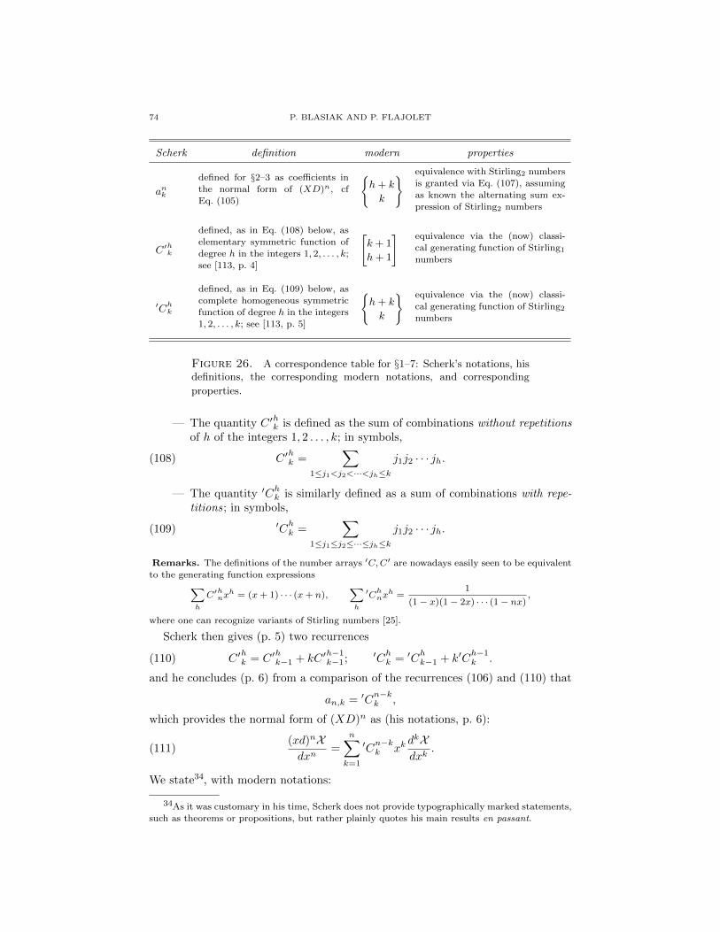
74 P. BLASIAK AND P. FLAJOLET
Scherk definition modern properties
ank
defined for §2–3 as coefficients inthe normal form of (XD)n, cf
Eq. (105)
{h+ k
k
} equivalence with Stirling2 numbers
is granted via Eq. (107), assuming
as known the alternating sum ex-pression of Stirling2 numbers
C′hk
defined, as in Eq. (108) below, aselementary symmetric function of
degree h in the integers 1, 2, . . . , k;see [113, p. 4]
[k + 1
h+ 1
] equivalence via the (now) classi-
cal generating function of Stirling1
numbers
′Chk
defined, as in Eq. (109) below, ascomplete homogeneous symmetric
function of degree h in the integers
1, 2, . . . , k; see [113, p. 5]
{h+ k
k
} equivalence via the (now) classi-
cal generating function of Stirling2
numbers
Figure 26. A correspondence table for §1–7: Scherk’s notations, hisdefinitions, the corresponding modern notations, and corresponding
properties.
— The quantity C ′hk is defined as the sum of combinations without repetitions
of h of the integers 1, 2 . . . , k; in symbols,
(108) C ′hk =
∑1≤j1<j2<···<jh≤k
j1j2 · · · jh.
— The quantity ′Chk is similarly defined as a sum of combinations with repe-
titions; in symbols,
(109) ′Chk =
∑1≤j1≤j2≤···≤jh≤k
j1j2 · · · jh.
Remarks. The definitions of the number arrays ′C,C′ are nowadays easily seen to be equivalent
to the generating function expressions∑h
C′hnx
h = (x+ 1) · · · (x+ n),∑h
′Chnx
h =1
(1− x)(1− 2x) · · · (1− nx),
where one can recognize variants of Stirling numbers [25].
Scherk then gives (p. 5) two recurrences
(110) C ′hk = C ′
hk−1 + kC ′
h−1k−1; ′C
hk = ′C
hk−1 + k′C
h−1k .
and he concludes (p. 6) from a comparison of the recurrences (106) and (110) that
an,k = ′Cn−kk ,
which provides the normal form of (XD)n as (his notations, p. 6):
(111)(xd)nXdxn
=
n∑k=1
′Cn−kk xk
dkXdxk
.
We state34, with modern notations:
34As it was customary in his time, Scherk does not provide typographically marked statements,such as theorems or propositions, but rather plainly quotes his main results en passant.

COMBINATORIAL MODELS OF CREATION–ANNIHILATION 75
Proposition A.1 (Scherk [113, p. 6]). The normal form of (XD)n is given by
(XD)n =
n∑k=1
{n
k
}XkDk, n ≥ 1.
§3. Scherk continues (pp. 7–8) with various considerations related to setting X =−x(1−x)k−1 followed by the substitution x = 1. His goal is to obtain a new proof ofthe normal form result (111). He also rederives in this framework the relation (107)directly from the definition of the ank .
§4. We now come to another problem, namely, that of the reduction of
(exD)nX .The coefficients35 bnk are determined by the normal form (p. 9):
(112) (exD)nX = enxn∑k=1
bnkDkX
Scherk then derives a recurrence to be compared to our Equation (110), from whichthere results (p. 10) that
bnk = C ′n−kn−1 .
Thus the bnk are now recognizable as Stirling numbers of the first kind. We state:
Proposition A.2. The normal form of (exD)n is given by
(exD)n = enxn∑k=1
[n
k
]Dk.
The section concludes with representations of Stirling1 numbers in terms of (sortof) generalized harmonic numbers.
§5. This section digresses from the main course of the dissertation (p. 14) andis admittedly only loosely related to the other sections. The problem consists infinding the laws of the derivatives of a composite function. The formula, com-monly attributed to Faa di Bruno (born in 1825(!), publication dated 1850), figuresexplicitly (p. 14); see [25] for a statement. Scherk says:
expressionem quamdam invenimus,qualem frustra in multis libris jamseapius quaesiveramus, quam itaquepaucis verbis hic tangere liceat.
we have discovered a certain formula,which we have very often tried in vainto find in books, so that we feel allowedto devote a few words to its description.
We refer to the scholarly study of Warren Johnson [69], regarding the history ofthis formula, which was once considered a basic component of combinatorial anal-ysis. Nowadays, via generating functions, the computation of the nth derivativeof a composite function f(g(z)) amounts to nothing but the determination of acoefficient,
n! [zn]
n∑j=0
fjj!
(n∑k=1
gkzk
k!
)j;
i.e., it is a simple avatar of the multinomial formula.
35In fact, Scherk also denotes the new coefficients by an,k; we adopt a different convention for
clarity.

76 P. BLASIAK AND P. FLAJOLET
§6. Scherk now considers (p. 15) the inverse problem: how to express the deriva-tives DnX in terms of the quantities (xD)nX and (exD)nX . His main formula is(p. 18)
(XnDn)X =
n−1∑h=0
(−1)hC ′hn−1(xD)n−hX .
and a parallel one serves to express enxDn in terms of the powers (exD)j , this timeby means of the Stirling2 numbers (his ′C). In retrospect, these two formulae aremanifestations of the fact that the matrices of Stirling1 and Stirling2 are inverse ofeach other. Scherk can then conclude that the coefficients C ′ serve to make explicitthe law of the successive derivatives of 1/(x log x) (p. 18) and log log x (p. 19, top):
dn
dxnlog log x =
(−1)n−1
xn
(n−1∑k=0
[n
k + 1
]k !
(log x)k+1
).
§7. This section gives two further consequences (p. 20) of previous developmentsincluding a formula which expresses the expansion of a function g(z) in terms oflog z, when z is near 1.
§8. The purpose is now to come back to the general problem (p. 20) of the reductionof (yD)n. Naturally, large symbolic expressions are available, for small n, involving
y, y′, y′′, . . . (The notation used in the memoir is yi
= y(i).) A typical formula (p. 20)
reads:
(yd)4Xdx4
=(yy′
3+ 4y2y′y′′ + y3y′′′
)X ′ + (7y2y′2 + 4y3y′′)X ′′ + 6y3y′X ′′′ + y4X ′′′′.
A discussion of the combinatorics of the coefficients occupies the next few pages(pp. 21–27). Naturally, the previously considered cases y = x and y = ex providevarious checks. The corresponding coefficients are denoted by υkn (written as usual
askυn
in the memoir). Scherk deduces various qualitative results on the shape of
a general expansion: he obtains exact values for the first few coefficients as wellas some infinite classes of particular coefficients. He then concludes regarding apossible discovery of the general law: .
Solutio itaque ideo tam difficilis factaest, quod disquisitionem coefficientiumnumericorum ab inventione singulorumterminorum ipsorum segregare non po-tuirimus.
Then, the process has become so un-tractable that we could not succeed withan investigation of all the numerical co-efficients, based on the sole discovery ofsome individual terms.
Remarks. The symbolic problem is indeed difficult. From the solution described earlier, in our
Section 6, we now know the following.
(i) The coefficient of X (r) in (yD)nX is obtained from the set of unordered r-forests of
(rooted, non plane) increasing trees having a total size of n, by assigning to a vertex of
outdegree j a weight equal to y(j); see Figure 27. (Trees are taken “unordered” (i.e.,non-plane) owing to the fact that y(x) is here an exponential generating function.)
(ii) Symbolically, one should proceed as follows, for an expansion of (yD)nX :
— Start from y(x) =∑j yjx
j/j!, so that yj plays the role of y(j).
— Compute 1/y(x), which involves a series of multinomial expansions.— Integrate the previous expansion, which only involves a substitution xn 7→ xn/n
for each n: we get in this way Φ :=∫y−1.

COMBINATORIAL MODELS OF CREATION–ANNIHILATION 77
Figure 27. Left : An illustration of the correspondence betweenScherk’s expansion of (yD)nX and forests of trees (case n = 4). Right :the decoration of a particular tree by the derivatives of y
— Take the compositional inverse of the preceding expansion Φ—this, by the Lagrangeinversion theorem only involves a further sequence of multinomial expansions. (We
determine here the generating function T (x) of increasing trees.)
— Raise T (x) to the rth power (for the coefficient of X (r)), extract the coefficient of
xn in 1r!T r, and finally multiply this coefficient by n! since we are dealing with
exponential generating functions.
Barely half a dozen instruction suffice to implement the general procedure in a symbolic manipu-
lation system such as Maple. We can in this way verify, in a fraction of a second, the correctnessof the expansion relative to (yD)5X , in the form given by Scherk (p. 20). For the benefit of the
curious reader, here is the outcome of our program in the case of (yD)6X :
X1
(32 y3y0
3y12 + 34 y2
2y03y1 + y0y1
5 + 26 y2y02y1
3 + 11 y1y4y04 + 15 y3y0
4y2 + y5y05)
+ X2
(34 y0
4y22 + 31 y0
2y14 + 146 y0
3y2y12 + 57 y0
4y1y3 + 6 y05y4
)+ X3
(90 y0
3y13 + 120 y0
4y1y2 + 15 y05y3
)+ X4
(65 y0
4y12 + 20 y0
5y2
)+ 15X5y0
5y1 + X6y06.
§9. This section starting p. 27 contains a further combinatorial investigation ofthe general case, in the light of the special cases considered earlier in §2–4. Near theend, the author offers a brief discussion (pp. 29–30) of the particular reduction of(xpD)n. What he obtains is, in present day notations (we write cn,k for coefficients,which Scherk once more denotes by akn):
Proposition A.3 (Scherk [113, pp. 30–31]). The normal form of (XpD)n is givenby
(XpD)n = Xn(p−1)∑k
cknXkDk,
78 P. BLASIAK AND P. FLAJOLET
where the coefficients ckn satisfy
ckn =∑
1≤j1≤j2≤···≤jn−k≤k
[j1p]·[(j2+1)p−1]·[(j3+2)p−2] · · · [(jn−k+n−k−1)p−(n−k−1)].
§10. This section (pp. 31–36) contains formulae that the author obtained, notbeing at the time cognizant of similar works by the Bernoullis and Laplace. Theyare relative to Bernoulli numbers, hence they will not be discussed further here.
H. Niewodniczanski Institute of Nuclear Physics
Polish Academy of Sciencesul. Radzikowskiego 152, PL-31342 Krakow, Poland
E-mail address: [email protected]
URL: www.ifj.edu.pl/~blasiak
Algorithms ProjectINRIA-Rocquencourt
F-78153 Le Chesnay, France
E-mail address: [email protected]
URL: algo.inria.fr/flajolet