Genetic Algorithm-Based Combinatorial Parametric Optimization

for the Calibration of Traffic Microscopie Simulation Models

Tao Ma

A thesis submitted in conformity with the requirements for

the degree of Master of Applied Science in Transportation Engineering

Graduate Department of Civil Engineering

University of Toronto

O Copyright by Tao Ma April ZOO1

National Library H * l of Canada Bibliothèque nationale du Canada

Acquisitions and Acquisitions et Bibliographic Services services bibliographiques

395 Wellington Street 395. nie Wellington Ottawa ON Kt A O N 4 Ottawa ON K1A ON4 Canada Canada

The author has granted a non- exclusive licence allowing the National Library of Canada to reproduce, loan, distribute or sell copies of this thesis in microform, paper or electronic formats.

The author retains ownership of the copyright in this thesis. Neither the thesis nor substantial extracts fiom it may be printed or otherwise reproduced without the author's permission.

L'auteur a accordé une licence non exclusive permettant à la Bhliotheque nationale du Canada de reproduire' prêter, distribuer ou vendre des copies de cette thèse sous la fonne de microfiche/Eilm, de reproduction sur papier ou sur format électronique.

L'auteur conserve la propnéte du droit d'auteur qui protège cette thèse. Ni la thèse ni des extraits substantiels de celle-ci ne doivent être imprimés ou autrement reproduits sans son autorisation.

Genetic Algorithm-Based Combinatorid Parametric Optimjcration for the Calibration of Trafic Microscopic Simulation Models M.A.Sc. Thesis, April2001 Tao Ma Graduate Department of Civil Engineering University of Toronto

Abstract

This thesis outlines an irnplementation of Genetic Aigorithms to trafnc simulation

optkization and development of a program called GENOSIM, a Genetic-based

Optimizer for Tranic Microscopic simulation Models. GENûSIM is developed as a pilot

software that employs the state of the art in combinatonal parametric optimization to

automate the tedious task of calibrating trafnc simulation models. The employed global

search technique, Genetic Algorithnis, is integrated with a dyoamic traEc microscopie

simulation modeler, Paramics, and experimented with Toronto network, Canada. The

output of GENOSIM is the near-optimal values of its car-following, lane changing and

dynamic routing parameters. Obtained results are promising.

Paramics consists of high performance cross-linked traffic models having multiple user-

adjustable parameters. Genetic Algorithm in GENOSIM will manipulate the values of

control parameters and search an optimal set of values as staxting configuration for these

parameters by matching mode1 outcome with observed data. The most of C* codes

s h o w here have been sùnplified for clariîy.

Dedicated to

m y beloved wife, WENLI GAO

and

my lovely daughter, MINGJTE MA

iii

1 would like to express my sincere gratitude to m y supervisor Professor Baher Abduihai

for providing invaluable guidance and constant inspiration, which made m e corne to be

fascinated with Genetic Aigorithms and have developed the combinatorial parametric

optimization software, GENOSIM.

1 also want to express rny appreciation to Professor Eric Miller who reviewed the thesis

and gave valuable comments, which is significant to future research.

Thanks to OGSST for funding my graduate study and research.

1 dso extend many thanks to my parents and brother Dr. Ying Ma and those who ever

offered me any help and support during the course of this research.

Table of Contents

1 Introduction ......................................................................... . . 1.1 Problem Description ..............................................................

1.1.1 Paramics .....................................................................

1.1.2 ITS and Microscopie Simulation ........................................

1.2 Mode1 Calibration or Combinatorid Parametric Opthkation ..............

1.2.1 Conception ..................................................................

1.2.2 Significance .................................................................

1.3 Sensitivity to Parameter Selection ...............................................

. ................................ 1.4 The Proposed Approach vs Literature Review

1 -5 Motivation of GENOSIM Development ........................................

2 Genetic Algorithms ................................................................

2 . 1 Introduction .........................................................................

2.2 Advantage in Combinatorid Parametric Optimi7iition ........................ . . 2.3 Conception and Pmciples .........................................................

2.3.1 Representations ......... .... ................................................

2.3.2 Algorithms ..................................................................

........................................................... 2.3 -3 Selection Schema

2.3.4 Operators .....................................................................

......................................................... 2.3.5 Control Parameters

3 GENOSIM Design and Implementation ..................................

3 -1 Interna1 Structure and Interface Design .......................................... 25

................................. 3.1.1 Hierarchy Structure of GA Components 25

3.1.2 Interface Design ............................................................ 41

3.2 integration of GAS with Paramics ................................................ 43

3.3 Experimental Comparison ......................................................... 45

3.3.1 Experimental Data ...................................................... 45

3 .3.2 Different Scenarios.. ....................................................... 46

3 .3.2.1 Objective Function Selection ............................................ 46

3 .3.2.2 Comparison of Four Types of GAS ..................................... 52

3.3.2.3 Comparison of Two Representations ................................... 55

3.3.3 Conclusion .................................................................... 56

4 GENOSIM Application in Real Case Study ............... .. ........... 57

4.1 Network and Experimental Description .......................................... 57

4.2 Random Seed Selection ............................................................. 58

4.3 GAS Configuration ................................................................... 60

................................................................................. 4.4 Results 61

5 Conclusion .............................................................................. 66

5.1 Summary of Research ......... .... ... ,. ...................................... 66

5.2 GENOSIM Contribution and Characteristics .................................... 66

5.3 Future Research Direction .......................................................... 67

Reference ......................... .- ...................................................... 68

Appendix A - Glossary ............................................................... 71

List of Figures

1 . 1 Sensitivity of Parameter (Mean Headway) to Simulation Output ..............

1.2 Sensitivity of Parameter (Mean Reaction T h e ) to Simulation Output .......

1.3 Sensitivity of Parameter (Feedback) to Simuiation Output .....................

1.4 Sensitivity of Parameter (FamilÏanty) to Simulation Output ..................

1.5 Sensitivity of Parameter (Perturbation) to Simulation Output ..................

1.6 GUI for Link and Lane Parameter Calibration ...................................

1.7 Logic Flow of Mode1 Parameter Calibration ......................................

2.1 Any Point Crossover ..................... .... ........... ,....

2.2 Mutation at Random Bits .................... ... .. .. ....... .. .. .. .............. 3.1 Hierarchy Structure of GAs' Components ........................................

3.2 GENOSIM Graphic User Interface ...............................................

3.3 Flow of Integration of GAs and Paramics .........................................

3 -4 Testbed Network for GENOSIM Design ..................... ,.,. ..............

3.5 Link Count Comparison Using Point Mean

Absolute Error (PMAE) Objective Function .....................................

3.6 Turn Count Comparison Using Point Mean

Absolute Error (PMAE) Objective Function ....................................

3.7 Link Count Comparison Using Global Relative

Error ( G E ) Objective Function ............................ ... ..................

vii

3.8 Tum Count Comparison Using Global Relative

................................................... Error (GRE) Objective Function

3 -9 Link Count Comparison Using Point Mean

...................................... Relative Error (PMRE) Objective Fmction

3.10 Turn Count Cornparison Using Point Mean

...................................... Relative Error (PMRE) Objective Function

3.1 1 Link Count Comparison Using Theil's Inequality

............................................. Coefficient (TIC) Objective Function

3.12 Tum Count Comparison Using Theil's Inequality

............................................. Coefficient (TIC) Objective Function

............................... 3.1 3 Convergence through Generations (Simple GA)

.................... 3.14 Convergence through Generations (Steady-State GA) .... ........................... 3.1 5 Convergence through Generations (Crowding GA)

......................... 3.16 Convergence through Generations (Kncremental GA)

............................ 4.1 Port Area in Toronto ... ................................

.................................. ...................... 4.2 Random Seed Selection ,..

4.3 Convergence through Generations (SSGA) ......................................

............................ 4.4 Convergence through Generations (Crowding GA)

4.5 Cornparison of Link Count Using Steady-State GA ................... ... ....

4.6 Cornparison of Turn Counts Ushg Steady-State GA ...........................

........................... 4.7 Cornparison of Link Counts Using Crowding GA ....

............................... 4.8 Comparison of Tum Counts Using Crowding GA

List of Tables

........................................ 1.1 Sensitive of Parameters to Model Output

..................... 3.1 GA Configuration for testing different objective fbnctions

3.2 Experimental Cornparison of Four Candidate Functions ........................

3.3 Configuration Iôr Different GAs Cornparison ....................................

3.4 Opthkation Result Cornparison Using Different GAs .........................

3 -5 GA Configuration for DSerent Representation Cornparison ..................

3 -6 Cornparison Result of Two Representations in Two DifYerent GAs ...........

................................ 4.1 GRE Fluctuation by Using Dinerent Seed Value

4.2 GA Run-Time Configuration in Real Case Study ................................

....................................... 4.3 Results of GA Evohtion ... ............ 4.4 Optimal Value of Calibrated Parameters ..........................................

4.5 GA Performance Cornparison ..................... .... ............................

Chapter 1 Introduction

1.1 Problem Description

Numerous problems in engineering require either maximizing a system's performance or

minimizing a "misfit" function. ''Misfit'' is used here to denote the error between the

model output and observations for the real systems Cl]. An overail system model consists

of a set of cross-linked sub-models that depend on a large number of parameters.

Opthkation of model performance involves the selection of the 'best' set of values for

the parameters. Best values (loosely interpreted as optimal) c m be obtained using genetic

algorithms, achieving a combinatorid optimiir;ition of paranieten of the target system

(micxosimulation) through minimizing a misfit function. Problems such as these pose a

great challenge due to the large parametric space to be searched. The search space is

usuaIly a multidimensional one where the values of the parameters c m be conceived as

coordinattes, and the 'fitness' representing goodness of fit as a hiUy surface. The process

of seeking an optimum point, either a global or the best attainable local optimum point,

involves some systematic search methods.

A very common optimkation challenge is how to thoroughly traverse the whole search

space to get to a global peak in case of unevedy distributed, non-uniform, muitipIe-peak

space. To solve such problems, one probably resorts to either traditional aualytical

gradients or numerical search methods. Due to various complex reasons, the traditional

methods may fail to achieve good results. In the recent years, Genetic Algorithms have

gained popularity as a generic, systems independent opiimbtion tool [2] [3] and have

shown to do quite welI.

1.1.1 Paramics [4]

Paramics is a suite of high performance cross-linked trafEc models that interact to

replicate the urban and highway road network and sirnulate movement and behavior of

individual vehicle in the vimial replica of a physical roadway network. Paramics models

a trafic network microscopicalIy at the individual dnver/vehicle level ufilizing car-

following, lane changïng and gap acceptance etc models. These models have multiple

user-adjustable parameters by which the modeler may adjust the simulated driving

behavior and e v h t e the performance of the network undet different scenarios. Any

change in one control parameter may cause network-wide cross-effects through the

linkage c h a h and can result in different model output. Paramics takes as input the virtuai

physical network and decisions parameter values and outputs the correspondhg network-

wide vehicular rnovernents. To accompiish redistic traffic simulation, parameters that

govern vehicle movement and behavior in the simulation models need to be calibrated

using a systematic approach.

By simuiating the movement of aU individuai vehicles through the network, a second-by-

second image of the state of the network is produced This provides engineers and

planners with detailed information on the average, range and tirne-variation of t r a c

conditions. In addition, the vehicle carries a set of parameters (currently about 75) that

d e h e the physical and behaviod characteristics of the driver-vehicle unit @VU). This

deîaiied level of parameterkation allows the complexity of a real traeic system to be

modeled far more accurately. Paramics hcludes a sophisticated micloscopic car-

following, gap acceptance and lane-changïng model. Dynamic and intelligent routing are

also modeled. Paramics development cycle is summarized in the following seven steps:

(1) Create a new Paramics network and embed a template road geometry file

(2) Build a road network by adding nodes, links and zones and coding detailed lane and

junction descriptions.

(3) BuiId demand matrices fiom origin/destination data and including fked demand data

such as bus routes.

(4) Assign traffic using an appropnate assignment technique.

(5) Collect and analyze model results.

(6) Calibrate base conditions by comparing model results to observed data.

(7) Vaiidate the base model against independent data

As with all trafic models each of the above stages requires checking and validation.

Usually checking consists of cornparisons of model results to observed data e.g. link

flows, queue lengths, joumey times etc. However, Paramics also d o w s the user to

visualize the movement of individual vehicles through the network and this c m lx

compared to videos fiom site or to local knowledge of how the network operates. This

gives a mixture of quantitative and qualitative analysis.

1.1.2 ITS and Microscopie simulation

ITS or Intelligent Transportation Systems is the study of how to explore and exploit the

opportunities where the advanced communication and transportation technology could be

potentidy and possibly integrated. Thus it is possible to improve the performance of

tdf ic ffow on congested network, provide travelers with efficient e c real-time

idionnation, and coordinate the provision of alternative modes of transport.

Intelligent Transportation Systems and modem urban road network design require more

insight and knowledge of the constitutive properties of trafoc systerns. Such knowledge is

needed to predict, through numerical simulations, the behavior of the vehicles under

physical conditions. Reliable predictions aliow for meeting the engineering requirements

at a lower cost Therefore, various tranic models have been developed to des-cribe the

driving behavior as much detailed as possible. However, Paramics, a comprehensive

visualization and microscopic M c simulation model, displayed distinguished features

and filled the gap as a key component of the solution and is getting more and more

popular nowadays. Through microscopic simulation, individual vehicle-driving behavior

couid be observed and analyzed in the network-oriented conte- In order to replicate real

world as accurately as possible, the grouping parameter values need to be determined so

that the simulation output is valid, reasonable and reliable. The identification of

combinatorid parameters for the simuiator's intemal models has corne to be a major

issue.

1.2 Mode1 Caiibration vs. Combinatorial Parametric Optimization

1.2.1 Conception

The o v e d traffic simulation model is a microscopic description of underlying driving

behavior, via a set of internai models with a number of parameters. By changing

parameter values, the simulation outcome will be different. Generally, the quality of

simulation and parameter specification can be evaluated by comparing, under given

experimental conditions, observed data fiom the real network (field counts) with

simulation results. The simulation is said to be accurate if the error between the

simulation results and the observed data is s m d enough. It is robust ifa slight change in

the experimental condition resuit in minimal oscillations in the simulated result 151.

Therefore, the definition of parameter calibration or optïrnïzation here refers to

minimizing the "misfit" by fine-tuning parameter values, thus Rdjusting simulation

results. By iterative search using genetic aigorithms, combinatorid parameter values

codd be eventually optimized so that discrepancy between the real system and its virtuai

replia is minimized.

1.2.2 Significance

Once parameters are found that adequately f i t modeled to real systerns' output, then the

models can be applied in several ways. It could be used as a summary way of descnbing

reality, to make reliable predictions about =er yet unobserved data, and perhaps even

to give explicative power to the model to formulate efficient policy, evaiuate different

scenarios and aid real-time traffic control and operation.

1 3 Sensitivity to Parameter Selection

Two elemtntary factors are taken into account for parameter selection. One is to select

those that have significant effect on model output. The other is to consider those that

6

closely relate to and prominently affect vehicle-drïving behavior and dynamic route

choice models.

In micro-simulation models in general, and in Pararnics parameter pool, the magnitude of

effect on driving behavior and network performance arising fiom different parameters are

significantly different Therefore, appropriate or inappropriate choice of decision

parameters can vastly e e c t the final network performance, as measured by a relevant

objective or fitness fünction.

On the other han& one chromosome in GA represents a candidate solution, e-g. a set of

parameters in our case, and is encoded in a binary bit string format The length of the

binary string is proportionai to the number of parameters encoded in one chromosome.

Too large length of binary string will heavily slow-down the GA iterative search speed

and increase computational cost. For these reasons, attention should be focused on those

parameters to which the fiîness function is most sensitive. Therefore, the GA

optimization could be carried out with reasonable population sue and number of

generations. Also, since we select parameters with relatively higher impact on overali

performance, good improvements of the fitness function could be reaiized within fewer

generations, fewer function evaluations and fewer runs of simulation.

In this research, five top sensitive parameters are selected for calibration: mean headway,

mean reaction time, perturbation, feedback and familiariîy. The fkst two parameters

influence network wide vehicle-driving behavior, the other three, perturbation, feedback

and f d a r i t y , are key parameters that enable routes to be updated dynamically in

response to ITS or network conditions. The five parameters are defined as follows:

(1) Mean headway is the average time between leading edges of successive vehicles.

(2) M e a . reaction time is the tirne taken by driver to Mplement any action through the

simulation penod. (e-g. car following, gap acceptance . . . etc.)

(3) Perturbation is a factor used to randomize the route-cost perception to effect

stochastic route choice.

(4) Feedback is a loop mechanism used to update travel t h e costs for equipped cirivers

throughout a simulation period in order to innuence route choice.

(5) Familiarity is also a factor describing the composition of the driver with

respect to their different levels of knowledge of the network with network details and

rat mm, dtimately affecting route choice.

In Parâmics, the default value of parameters are mean headway = 1.0 sec, mean reaction

time = 1.0 sec, perturbation = 5%, feedback = 300 sec and familiarity = 85%. Each

parameter has been ïndividually tested for its sensitivity to the fluctuation on model

output. In each experiment, only the value of one of five parameters has been changed so

that it is different fiom its default value and the other parameters are kept on default

values. The table 1.1 summarizes the experimental results, which indicate the sensitivity

of these parameters to model output.

Parameters

'~eedback (Fd = 60 sec) 51.31 % 70.82% Familiarity (Fa = 45%) 49.40% 66.85% 'Perturbation (P = 60%) 74.57% 83.66%

Table 1.1 Sensitivity of Parameters to Mode1 Output

The figure 1.1 - 1.5 show the changes in link count by adjusting

experimental data is explained in 3.3 Chapter 3.

parameter vdue. The

Sensitivity of Parameter (Mean Headway) to Simulation Output

Defautt (1 .O Sec) - -n - - Mean Headwy 0.5 Sec

Figure 1.1

Sensitivity of Parameter (Mean Reaction Tirne) to Simulation Output

- Defauit (1 .O sec) - -= - - Mean Reaction Tirne (0-4 Sec) 1

1 6 11 16 21 26 31 36 41 46 51 56 61 66 71 76

Locations

Figure 1.2

-

Sensitivity of Parameter (Feed back) to Simulation Output

1 - Defaut (300 Sec) - -S - - Feedbac k (60 sec)

Locations l

Figure 1.3

Sensitivity of Parameter (Familiarity) to Simulation Output

Figure 1.4

Sensitivity of Parameter (Perturbation) to Simulation Output

i 1 - Default (5%) - -S - - Perturbation (69%) 1

1 6 11 16 21 26 31 36 41 46 51 56 61 6ô 71 76

Locations

Figure 1.5

1.4 The Proposed Approach vs- Literature Review

In Paramics documents, it was suggested that calibration is an essential stage of the t d i c

modeling process. Usually this procedure requires comparing model results to observed

data and ensuring that these comparisons fd within acceptable guideluies.

As part of model calibration the visualization of traffic moving through the road network

may be compared to junction video information or local knowledge of tnd3c operation.

In addition, the output statistics such as tuniing count, link count, journey times and

queue length etc. can be collected and compared to data obsenred on site-

The calibration procedure for Paramics involves standard checks that are carried out to

verify vehicle routing, trafnc demand matrices, road layout details etc. After complethg

these checks and verifyuig they are acceptable, the user must output model statistics for

comparison to observed data Comparisons between modeIed and observed data should

include some of the following assessments: trafnc flows, queue lengths and stop rime

delays, traffic speeds, traffic density, and joumey times. Modeled routing compare to an

assessment of actual routing. If the observed to modeled comparisons are within

recommended guidelines and the visuaikation of the vehicles is realistic, then the model

is deemed to be calibrated- However, if the comparisons are unacceptable then the user

should carry out further analysis to

a Assess traffic assignment

Check road geometry (visiialiiration)

Check routes

Checkobserveddata

Check tmflic demand

The checking procedure should identifil any coduig errors that can be quickly rectifkd

using the editor fiinction. The updated model is then re-run and results are collected and

analyzed. The process is repeated mtil good calibration is achieved.

If the model still gives inaccurate simulation then the user may wish to change some

default parameters coded in Paramics to model the behavior of individual driver vehicle

uni& (DVZT). Usually, the major adjustments to a model include moving kerb and stop-

line control points, and coding forced lane changes to ovemde default Paramics lane

changing. The main iink, lane, and junction calibration parameters include

(refer to figure 1.6)

8Changing the hazard warning distance

8Including link gradients

8Coding junction visibility

8Changing link headway factor

Coding link end speeds

ZCodhg lane endstop t h e

ZForced lane changes

ZForced merges

ZStay in lane

&Lane and tuni restrictions Figure 1-6 GUI for Link and Lane Parameter Calibration

Overd, above Paramics documents do point out how to consider or cary out the

calibration, either by correcting the network-input error or t-g some parameters.

However, it didn't propose any efficient systematic method for calibration. AU the ways

mentioned above have to be done manually by graphic user interface. ActuaIIy, in real

projects, it's impracticd to do calibration manuaily. Therefore, an efficient and realistic

solution has to be formulated so that calibration could be implemented automaticdy

instead of manually.

The trial and error method was applied to this same problem in 1998 [a in Irvine USA.

In 2000, the use of the Genetic Algorihm for Paramics parameter calibration was

proposed and explored on a short fkeway Link, within Paramics' Application

Programmïng Interface (API) [q. In that case, only two drivuig parameters were

calibrated without inclusion of any routing parameters and without füli automation. An

elaborate application of genetic aigorithms and full automatic mechaaism are stiLl absent

ho wever.

It has been proven by many decades of experience and practice of optimktion research

that Genetic Algorithms is an extensively used search technique that borrows ideas fiom

natural evolution to effectively find good solutions for combinatorid parametrïc

ophizaîion problems. Therefore, GENOSIM is created as an independent optimization

tool that externaiiy links to any simulation environment, thus having a potentid of

interacting with simulation environments other than Paratnics.

As described in Figure 1.7, the rnisfit is evaluated through the difference between the

observeci data and simulation outcorne. The term 'optïmization' is loosely used here to

14

indicate finding parameter values for the simulation models that rninimize the misfit

hction. However, genetic algorithnis do not necessarily guarantee global optimality in

the mathematical sense.

Figure 1.7 Logic Flow of Mode1 Parameter Calibration

1.5 Motivation of GENOSIM Development

Our interest in using Genetic Algorithms to tackIe combùiatorial pararnetric optirnization

problem is motivated by the need for a systematic approach to calibrate the increasingly

popular traffic micro-simulation models for InteUigent Transportation Systems (ITS)

applications, thus offering an automated optimization tool for microscopic simulation

parameters. However, the process suggested in Paramics documents seems to be

impractical, because users have to keep on fine tuning parameter values manuaUy to fit

the simulation output with obçerved data In order to implement an idea that automates

mode1 caiibration, GENOSIM, a Windows-based program, has been developed in Cst.

By using it, the user can easily and automatically optimUe the parameter values for the

simulation model.

In this thesis we introduce and describe GENûSIM: a Genetic Algorithms-based

simulation-optimization system. The objective of GENOSIM is to search for optimal

configuration for microscopie simulation parameters in order to minimize discrepancy

between simulation output and real field conditions.

Chapter 2 Genetic Algorithms

2.1 Introduction

". ..the metaphor unddying genetic algorithms is that of natural evolution. In evolution,

the problem each species faces is one of searchiag for beneficial adaptations to a

complicated and changing environment, The 'knowledge' that each species has gained is

embodied in the makeup of the chromosomes of its members." [15]

During past three decades, the grown demand on combinatorid optimbtion problems

put genetic algorithms in a significant position. Genetic Aigorithms have been quite

widely and successfülly applied to numerous optimi7ation problems Wce wire routing,

scheduling, adaptive control, game playing, cognitive modeling, transportation problems,

traveling salesman problems, optimal control problems, database query optimization, etc.

Genetic Algorithms (GAs) are a stochastic search method based on the principles and

mechanisms of natural selection and 'survival of the fittest' fiom natural evolution, GAs

has corne to be a popdar optirniidon rnethod since htroduced in 1970s by Hoiland's

study of adaptation in artScid and natural systems CS]. By simulating naturai

evolutionary processes, a GA c m effectively search the problem domain thoroughly on

population-based solutions rather than a single solution, and employ heuristics to evolve

better solution. The facility of restarting the iterative search fkom a wide variety of

starting points provides some safeguard against entrapment on a local optima, thus

making GAs prevail over conventional search methods.

A GA performs a mutil-directiod search by maintaining a population of potential

solutions and encourages information formation and exchange between these directions.

The population undergoes a simulated evolution: at each generation the relatively "good7'

solutions reproduce, while the relatively 'cbad77 solutions die. To distuiguish between

dinerent solutions, an objective fûnction is used for evaluation that plays the role of

environment,

2.2 GAs Advantages in Combinatorial Parametric Optimization

Various conventional optimization techniques have been developed and implemented in

practical applications, such as analytlcal methods (least mean-squares or maximum

likelihood estimates), various types o f hili climbing, randomized search and trial and

exror-

However, many models and their misfit hct ions cannot be expressed either in an

analyticaliy soluble form or with differentiable error fûnction suitable for gradient-guided

search techniques. Conventional approaches can therefore easily fail in obtaining the

global optimum in complex search space situations in practice. For rnany nich cases that

cannot be optimized analytically, various '‘bill-climbing" or 'Wey-descending"

techniques have been used to search toward an optimum in iteraîive loop. But, For

problems which have multiple local optima, boîh the iterative incremental step and

steepest descent methods lead to a dmger of entrapment on local optima and saddle

points. [l] In addition, some conventional opthkation methods suffer fkom lack of a

priori information on the systern parameters or cannot easily be applied to nonlinear

systems.

Genetic Algorithms have been found to be particularly effective and powerful in

exploring and exploithg poorly understood or non-dserentiable spaces for optimization

and machine learning. It has also been successfully applied to systems identification and

parameter estimation [9][10]. For this type of problem, genetic algorithms have the

advantage that ali parts of the feasible space are potentially available for exploration and

exploitation. So the global optima stand beiter chance of being attained Overall, Genetic

Algorithms have unique advantages and charisma in solving the issues of combinatorid

paramebnc optimization.

2 3 Conception and Principles

The following is a brief description of key components of GA:

23.1 Representation

Chromosome: one distinct element in the GA is the chromosome that is encoded as a

single solution. A single solution here means one set of values of combinatorid

parameters for the simulation model. One chromosome is subdivided into genes.

Associated with each chromosome is a rnisfit value, which determines its chance to

survive and produce offspring.

Genes: a gene, a bit string, is a binary representation of a single parameter value, which

must have an upper and lower bound declared. The Iength of the bit string is of

paramount importance. It determines how precise a point the GA could reach in the

19

search space. The longer the binary bit string is, the better but at the expense of high

computation COS- In this research, a 16 or 8 bit is used for each gene to attempt to make

every possible point in the search space reachable nom the initial population through

genetic operators.

Real-Valued and Binary: The standard GAs are characterized by the use of the binary

coding for each string. However, in this paper, both real (decimal) and binary formats are

offered because, as pointed out by Wright (1991), rd-valued genes offer a number of

advantages in numerical optimi;ration:

(1) efficiency of the GA is increased, as there is no need to convert chromosomes

between binary and decimal before each h c t i o n evaluation

(2) Iess memory is required

(3) there is no loss in precision

(4) there is greater Eeedom to use difïerent genetic operators

(5) Real-valued GA can take advantage of higher mutation rate than binary coding,

thereby increasing the level of possible exploration of the search space.[ll] Cl21

The binary representation traditionally used in genetic algorithms has some drawbacks

when applied to multidimensional, high-precision numericd problerns. For example, for

100 variables with domains in the range [-500, 5001 where a precision of six digits after

the decimd point is required, the length of binary solution vector is 3000. This, in turn,

generates a search space of about 10'~~~. For such problems genetic algorithms perform

poorly 1141. In particular, for parameter optimization problem with variables over

continuous domains, real-number representation performs better than binary code. In

GENOSIM design, two types of representation have been implemented and examined for

their merence-

23.2 Algorithms

Although, there are many versions of genetic dgorithms, ail of them have two basic

steps: selection and replacement. The selection step determines how the parents are

selected for producing offspring. The replacement step determines how o f f s p ~ g s will be

inserted into the population and how old members are to be eliminated.

If the problem requires iteration on more than two parameters, then it may be very

difficult to check for local optima In order to avoid a danger of entrapment on local

optima or sadde points and to examine what type of GA is more efficient for

combinatorid parameter optimïzation, four types of GAs are implemented in GENOSIM:

simple GA, steady-state GA, crowding GA and incremental GA.

Simple GA (Non-Overlapping Popdations)

The simple genetic algorithm is a very cornmon implementation. It uses non-overlapping

populations. In each generation, the entire population is replaced with new individuals. If

the elitism mechanism is specified, the best individual will be carried over fiom one

generation to the next to increase converge speed. The best individuai is more likely to be

selected for mating [13].

Steady-state GA (Overlapping Populations)

The steady-state genetic algorithm uses overlapping populations. In each generation, a

portion of the population is replaced by the newly generated individuais. The steady-state

algorithm is another standard genetic algorithm, If only one or two individuds may be

replaced in each generation, it is so-cded Incremental GA. At the other exireme, the

steady-state algorithm becomes a simple genetic algorithm when the entire population is

replaced [13].

Crowding-Based GA

Crowding is a generalhtion of pre-selection. In crowding GA, selection and

reproduction are the same as in the SGA, but replacement is a distinct feature. Before

replacement, the new offsprïng will execute a comparison with individuals of the

population using a distance function as a measure of similarity. The popdation member

that is most similar to the offspring is replaced by the offspring. This procedure is

repeated. This strategy maintains the diversity in the population and slows down

premature convergence of the traditional G& thus making crowding GA prevail over the

others. In most cases, It can find the global optimum in a multi-dimensional search space

WI-

2 3 3 Selection Schema

Selection is the process of choosing two parents fiom the popuiation for exchanging

genetic materials. Four types of selection schemas have been hplemented hto

GENOSIM: roulette wheel, tournament, rank and iuiiform.

Roulette Wheel: Roulette selection is one of the traditional GA selection techniques. This

selection method picks an individual based on the magnitude of the fitness relative to the

rest of the population. A target value is set, which is a random proportion of the sum of

22

the fitness in the population. The population is stepped through until the target value is

reached This is only a moderateiy strong selection technique, since fit individuals are not

guaranteed to be selected for, but the higher the fitness, the more likely an individual will

be selected. Any individual has a probability p of being chosen where p is equal to the

fitness of the individual divided by the sum of the fitness of each individuai in the

population. It is essential that the population not be sorted by fitness, since this would

dramaticaUy bias the selection-

Tournament: The tournament selection uses the roulette wheel method to select two

individuals then picks the one with the higher fitness. The tournament selection typically

chooses higher valued individuals more often than the Roulette Wheel.

Rank: The rank selection picks the best member of the population every t h e .

Uniform: The stochastic uniform selection picks randomly from the population. Any

individual in the population has a probability p of being chosen where p is equal to 1

divided by the population size.

23.4 Operators

During the reproduction phase of genetic algorithm, there are two classicai genetic

operators: crossover and mutation.

Crossover: This operator creates new oEspring fiom the original parents. In this

implementation the parent chromosomes are grouped into pairs through selection

schemata and each of these pairs creates two child chromosomes by a process of

23

combination. The following two chrornosomes have been selected to exchange genetic

matenal and reproduce two new child chromosomes. (refer to figure 2.1)

Parent 1

Parent 2

Child 1

Child 2

Figure 2.1 Any Point Crossover

Mutation: This is the process of randody disturbing genetic information. The mutation

probabiüty determines the rate at which a gene of chromosome is altered. Mutation add

new information in a =dom way to genetic semh process, and uitimately help to avoid

GAs fiom getting stuck at local optimums. Mutation operates at the bit copy level; when

the bits are being copied from the parent to the chiid, there is a probability that each bit

may become mutated. The probability is usually set to a quite smail value. A coin toss

mechanism is employed; if a random number between O and 1 is less than mutation

probability, the bit is inverted, e-g. zeros become ones and ones become zeros. This

random scattering rnight h d better optima or even m o w a part of a genetic material

that will be beneficial in a later crossing. On the other hand it might produce a weak

individual that will never be selected for crossing. (refer to figure 2.2)

Child 1 1 1 1 1 1 1

Child 2

I

Child 2" ~ i i ~ i ~ i ~ ~ ~ I I

Figure 2.2 Mutation at Randorn Bits

23.5 Control Parameters

The population size, generations, probability of crossover, probability of mutation are the

control pammeters for GAs nia User configures the nin t h e setting for genetic

algorithm through s p e c w g these control parameters. The search process usudy stops

at the speczed number of generations.

Chapter 3 GENOSIM Design and Implernentation

3.1 Interna1 Structure and Interf'ace Design

There are many decisions to be made when designhg a problem-specific GAs. To some

extent, configuring a GA suitable to a particdar problem is an art.

3.1.1 Structure of Components

Currently, various Genetic Algorïthms and its components have been developed and

applied to dinerent specinc issues. Genetic Algorithms are regarded as a problem-

specifzc optimization method. In GENOSIM design for combinatorid parametric

optïmization, various scenarios have been implemented in chromosome representation,

algorithms, selection schemas and operators. Diffierent options are oEered and

experimental cornparisons have been made for different option combination. Eventually,

the suitable combinatonal option is recommended as a highly efficient and efficacy

configuration for the real case study. Meanwhiie, four objective functions have been

tested for accuracy and efficiency and the global relative e w r fiinction is employed in

the design as objective hct ion. Figure 3.1 shows hierarchy structure of genetic

algonthms designed in GENOSIM.

Representation (Real-Valued and Binary)

The two distinct elements in the GA are individuals and population. An individual is a

single solution. The population is the set of individuals currentiy involved in the search

process. A gene, a calibrated parameter, is a component of an individual and can be

represented either in a bi- code or real number. The binary representation is a bit

26

string of arbitrary length that indicates the number of intervais between a lower bound

and upper bound of the parameter. The range declared for a parameter is divided into the

number of intervals that is a fiinction of the Length of gene's bit string. A bit string of

length n can represent NI intervals b y following expression (equation 3.1):

NI = 2" - 1 ................... .. .........m.. 9. *** -99--9.9-. (3-1)

Hierarchy Structure of GA Components in GENOSIM

Representation

Real Number

Algorithms Simple GA Steady-S tate GA Crowding GA Incremental GA

L ~ e l e c t i o n Schema Roulettewheel Tournament Rank unif-onn

- Operators

-

- Crossover Uniform (Binary/Real) One-Point (BinaryiReai) Two-Point (Binary/Real) Blending (Real) Averaging (Reai)

-Mutation Bit-Fiip (Bïnary) Uniform (Red) Gaussian (Real) Boundary (Reai)

- Control Parameters Population Size Generations Probabiiity of Crossover Probability o f Mutation

Figure 3.1 Hierarchy Structure of GAs' Components

The size of the intemal would be SI by the following expression: (equation 3.2)

For example, Parameter A has a range of 0.5 - 2.0 and the bit string is eight bits in

length. This gives 255 intervals and an interna1 size of 0.00588. The bit string 'OOOOOOOO'

represents zero intervals so the gene's value is equal to the lower bound

0.5 + (O * 0.00588) = 0.5

The bit string ' 11 11 11 I l ' represents 255 intervals, so the gene's value is equal to the

upper bound,

The bit string '0 1 10 1 10 1 ' represents 109 intervals, so the gene's value is equal to

1.14092.

0.5 + (109 * 0.00588) = 1.1 14092

The size of the bit string is of paramount importance. If the interval is too coarse, the GA

may never be able to find an optima simply because the genes can't express a value close

enough to the optima Too fine a resolution may result in excessive hair splitting in the

search.

Selection Schema

/*

Roulette Wheel Selector

This seiection routine screens the members of the population through a weighted roulette

wheel. Likelihood of selection is proportional to the fitness score. It assumes that the

individuals are in order fiom best (0th) to worst (II-1). When the summation of fitness

before ith individual reaches the random target value, the (i-l)th individuai wiil be

selected. - */

RouletteWheel ( ) {

float Target;

int i, upper, lower;

Target = Population.SumFitness*Random(O,l);

lower = 1;

upper = Population. size ( ) ;

while (upper >= lower) {

i = lower + (upper-lower) /2; if (SumFit [il > Target)

upper = i-1;

lower = i+l;

1

lower = Min (Population. size ( ) , lower) ; lower = Max (1, lower) ;

return Population.indiuidual(lower);

Tournament Selector

Tournament method picks up two individuais fiom the population using the Roulette

Wheel selection method.. Then retum the better of the two individuals.

Tournament ( ) {

int pickl, pick2;

f loat Target;

int i, upper, lower;

Target = Population.SumFitnessfRandom(0,l);

lower = 1;

upper = Population.size0;

while (upper >= lower) I

i = lower + (upper-lower)/2; if (SumFit Ci] > Target)

upper = i-1;

else

lower = i+l;

1

lower = in (Population. size ( ) , lower) ; lower = Max (1, lower) ;

pickl = lower;

Target = Population.SumFitness*Random(O,l);

lower = 1;

upper = Population. size ( ) ;

while (upper >= lower) {

i = lower + (upper-lower) /2; if (SumFit [il > Target)

upper = i-1;

else

lower = itl;

1 lower = Min(Population.size(), lower);

lower = Max(1, lower) ;

pick2 = lower;

if (Population. individuai. (pickl) .score ( ) >

Population - individual (pick2) . score ( ) ) X = Population. individual (pickl) ;

else

X = Population. individual (p ick2) ;

return X;

/* - -- Rank Selector

This routine always retums the best individuai Gcom the population. Any population may

contain more than one individual with the same score. This method must be able to retum

any one of those 'best' individds.

----- - __I-- */

Rank0 {

int if count=l;

float Best [Population. size ( ) ] ;

Population. SortFitness ( ) ;

B e s t ( 1) = Population. individual (1) ;

for(i=2; i<Population.size();i++)(

if (Population. i nd iv idua l (1) - f itness ( ) ==

Population. individual (i) . fitness ( ) ) {

count+i;

Best (count ) = Population. individual (i) ;

1

1

r e t u r n Population.Best(RandornInteger(Ifcount));

i

/*

Unifonn Selector

Randomly select an individual h m the population.

* /

float Z;

int 1;

1 = RandomInteger (1, Population- si ze ( ) ) ;

Z = Population. individual (1) ;

return Z;

Operators

/* --VI - ----.-

Uniform Crossover

Randomly take bits fiom each parent. Flip a coin for each bit to see if that bit should

corne fkom the mother or the father. Assume strings have the same Iength.

Unif ormCrossover ( ) {

int i;

for(i=dauhter/son/mom/dad.length(); I>=1; i--){

if (Random(0 or 1) ) {

daughter. gene (i, dad. gene (i) ) ;

son,gene(i, morn.gene(i));

/* One-Point Crossover

Pick a single point then copy genetic material fiom each parent

*/

OnePointCrossover() (

unsigned int cutsite;

cutsite = RandomInteger(0, mom or dad-lengtho);

momsection = mon-length() - cutsite; dadsection = dad. length ( ) - cutsite; daughter. copy(mom, 0, 0, cutsite) ;

daughter. copy (dad, cutsite, cutsite, dadsection) ;

son. copy (dad, 0, 0, cutsite) ;

son. copy (morn, cutsite, cutsite, momsection) ;

k

/* --- - 4-- - - Two-Point Crossover

Two-point crossover is similar to the single point crossover, but randoxniy pick two

points then exchange the sections between those two points.

- - _ ---- -- - */

unsigned int cutsitel, cutsite2, trnp;

unsigned int midsection, lastsection;

cutsitel = RandomInteger(0, rnom or dad.length0 ) ;

cutsite2 = RandomInteger (O, mom or dad- l eng th ( ) ) ;

if (cutsitel > cutsite2) (

trnp = cutsitel;

cutsitel = cutsite2;

cutsite2 = tmp;

rnidsection = cutsite2 - cutsitel;

lastsection = mom.length() - cutsite2;

daughter - copy(mom, 0, 0, cutsitel) ; daughter,copy(dad, cutsitel, cutsitei, midsection);

daughter.copy(mom, cutsite2, cutsite2, lastsection);

son- copy (dad, 0, 0, cutsitel) ;

son. copy (mom, cutsitel, cutsitel, midsection) ;

son, copy (dad, cutsite2, cutsite2, lastsection) ;

/* - B lending Crossover

Recalcdate the boundary based on two parents' distance. Then generate new children

within new boundary. -- -- */

BlendCrossover ( ) {

for(int i=0; iCparent.length(); i++) {

float l o w = Min(mom.gene(i), dad.gene(i) ) ;

float hig = Max(mom.gene(i), dad.gene(i));

float distance = (float) (hig - low) /2.0; low -= distance;

hig += distance;

low = Max (low, lowerbound) ;

hig = Min (hig, upperbound) ;

child. gene (i, RandomFloat (low, hig) ) ;

/*

Averaging Crossover (Real)

Take the average of two parents' genetic material as children genetic material.

*/

AveragingCrossover ( ) {

float average;

for ( int i=O ; icparent . length ( ) ; i++) {

average = (mom.gene(i) + dad.gene(i))/2.0; average = Max (average, lowerbound) ;

average = Min (average, upperbound) ;

child. gene (i, average) ;

1

/* -- -- -------- Bit-Flip Mutation

If the mutation probability is smd, then we toss coin for each bit in the string see if that

bit mutate. Othenvise, simply mutate a known number of bits based on the mutation rate

and length of bit string.

BitFlipMutation ( ) {

float nMut = pmut * child.length(); if ( M u t < 1.0) {

for (i=child. length ( ) -1; i>=O; i--) {

if (TossCoin (pmut) ) {

child.gene(i, ((child.gene(i) == 0) ? 1 : 0));

else (

for(n=O; nCnMut; n++) {

i = Randornhteger (O, child, length ( ) -1 1 ;

child.gene(i, ((child.gene(i) -- 0) ? 1 : 0));

1

1

/ * Gaussian Mutation

Genetic material of an individual is replaced with a randorn number fkom Gaussian

distribution dehed by a mean and standard deviation. - -- */

GaussianMutation ( ) {

for(int i=O; i<individual.length(); i++) {

if (TossCoin (pmut) ) {

float new;

do I n e w = Gaussian(individual.gene(i) 1;

while (new C individual. gene (i) . lower ( ) I I n e w >

individual .gene (i) .upper ( ) ) ;

individual - gene (i, new) ;

Uniform Mutation

Genetic matenal of an individuil is replaced by a random number within declared

boundary.

UniformMutation ( ) {

for (int i=O ; i<individual. length ( ) ; i++) {

if (TossCoin (pmut) ) {

float new, l o w , h i g ;

low = individual. g e n e (i) . lower ( ) ; hig = individual. g e n e (i) . upper ( ) ; new = RandomGenerator (low, hig) ;

individual. gene (if new) ;

1

1

/* --- -- Boundary Mutation

The genetic material is replaceci either by lower bound or upper bound.

- C _ _ _ - - - - - - - - -- */

BoundaryMutationO {

for (int i=O ; icindividual . length ( ) ; i++ ) {

i f (TossCoin (pmut) ) {

f loat low, hig;

if(RandomC0,l) {

low = individual. gene (i) . lower ( ) ;

individual. gene (i, low) ;

1 else (

hig = individual. gene (i) . upper ( ) ; individual. gene (i, hig) ;

/* - - --- Simple GA

Evolve a new generation. M e n this routine strilts, population contains the current

generation. When finishes, population contains the new generation and old Population

contains the current generation. The previous old generation is replaced The best

individual in old Population will migrate into new generation. If supposed to be elitist,

migrate the best individual fkom the old population into the new population.

-- -- - */

SimpleGA() {

tmppopulation = oldPopulation;

oldPopulation = population;

population = tmppopulation;

for(i=O; icpop->size()-1; i+=2) {

mom = oldPopulation.select0;

dad = oldPopulation.select();

if (TossCoin (pcrossover ( ) ) ) {

GACrossOver(rnom, dad, population.individual(i),

1

else {

populatuon. individual ( i . copy (mom) ; population. individual (i+1) . copy (dad) ;

l population.individual( i ) .mutate(pMutation());

population.individuaI(it1) .mutate(pMutation());

1 if(popu1ation-size ( ) % 2 != 0) {

mom = oldPopulation. s e l e c t ( ) ;

dad = oldPopulation, select ( ) ;

i f (TossCoin (pcrossover ( ) ) ) {

GACrossover (mom, dad, population, individual ( i l , O) ; 1

else {

i f (Randomf lip ( ) )

populat ion. ind iv idua l ( i ) copy (moni) ;

else

populat ion. ind iv idua l ( i ) . copy (dad) ;

1 population. i nd iv idua l ( i ) .mutate (pMutation ( 1 ) ;

1

if (oldPopulation. best ( ) . score ( ) > popula t ion . best ( ) . sco re ( ) )

population. r ep lace (01dPopulation. best ( ) ) ;

1

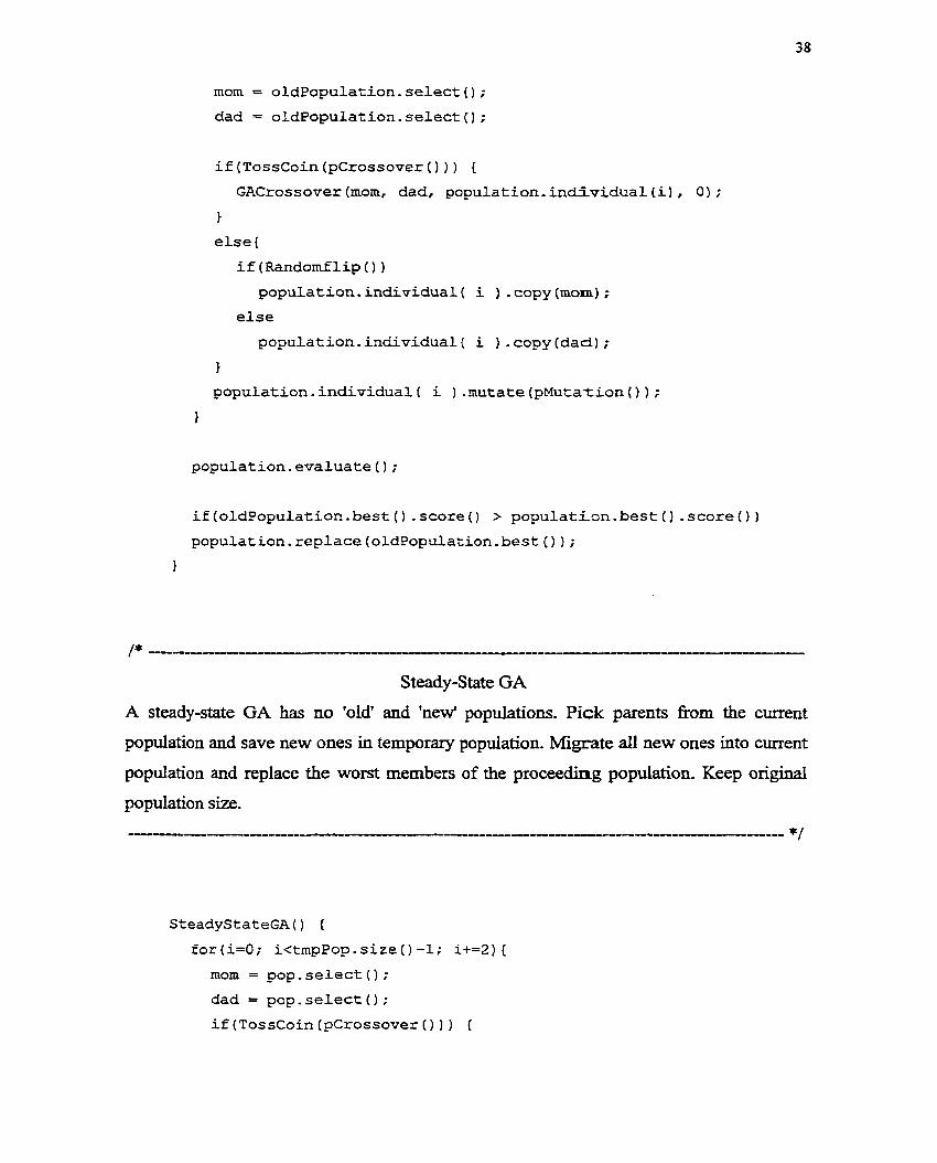
/* --------- --- P ---- Steady-State GA

A steady-state GA has no 'old' and 'new' populations. Pick parents f?om the current

population and Save new ones in temporary population. Migrate d new ones into curxent

popdation and replace the worst members of the proceeding population. Keep original

population size.

------i-i-U---------------- -~-~--------UI-C-UI~---C------ */

SteadyStateGA ( ) {

f o r ( i = O ; i<tmpPop. size ( ) -1; i+=2) {

rnom = pop. select ( 1 ;

dad = pop. select ( ) ;

i f (TossCoin (pcrossover ( ) ) ) {

GACrossover (mom, dad, tmpPop - individual (i) , tmpPop - individual (i+l) ) ;

1

else {

tmpPop.individual( i ).copy(rnom);

tmpPop, individual (i+I) . copy ( dad) ;

1

tmpPop. individual ( i ) .mutate (pMutation ( ) ) ) ;

tmpPop. individual (i+I) ,mutate (pMutation ( ) ) ) ;

1

if(tmpPop.size() 8 2 != 0) {

mom = pop-select ( ) ;

dad = pop. select ( ) ;

if (TossCoin (p~rossover ( ) ) ) {

GACrossover (mom, dad, tmpPop . individual (i) , 0) ; 1

else {

if (Randomflip ( 1 )

tmpPop . individual ( i ) . copy (mom) ; else

trnpPop. individual ( i ) . copy (dad) ; 1

tmpPop . individual ( i ) .mutate (pMutation ( ) ) ) ;

}

for ( i = 0 ; i<tmpPop . size ( ) ; i++) {

pop.add(tmpPop.individua1 (i) ) ;

1

pop. evaluate ( ) ;

pop. rernove (WORST, population. size ( ) ) ;

/* - Crowding GA

Clone current members into mating pool, pick parents fkom mating pool and remove

them fiom the pool. Create new children and compare with the parents. Then r e m

higher fitness members to population.

- */

CrowdingGA ( ) {

for (int i=0; icpop-size ( ) ; it+) {

matingpool . clone (i) ; 1

do {

mom = pop.Randomindividual();

matingpool . rernove (mom);

dad = pop, Etandomindividual( ) ;

matingpool, rernove (dad) ;

GACrossover (mom, dad, child, 0) ;

Child-mutate (p~utation ( ) ) ;

float dl = child. compare (mom) ;

float d2 = child. compare (dad) ;

FitnessStrategy --= minimize;

if (dl < d2 & & ) {

if (child. score ( ) C mom. score ( ) ) {

mom. copy ( child) ;

1

1

else {

if (child. score ( ) < dad. score ( ) ) {

dad . copy ( child) ; 1

1

1 while (matingpool. size ( 1 >1) ;

pop - evaluate ( ) ;

/* -- hcremental GA

Similar to a steady-state GA. Pick parents fiom the current population and replace its

members with the new ones created. Only generate two children in each generation. The

replacement strategy is set by the GA (either replace their parent or the worst member).

*/

IncrementalGAO {

mom = population.select();

dad = population.select();

if (TossCoin (pCrossover ( ) ) {

GACrossover (mom, dad, childl, child2) ;

else {

c h i l d l . copy (rnoml ; child2. copy (dad) ;

1

childl .mutate (pMutation ( ) ) ;

chi ld2 .mutate (pMutation ( ) 1 ;

childl = population.replace(childl, replacementstrategy);

child2 = population.replace(child2, replacementstrategy);

3.1.2 Interface Design

GENO S M , a standard Windows-based application, has graphic user interface (GUI). To

execute the optimhtion process, the user needs to follow two steps. First step is to set up

the run-tirne codiguration for genetic algorithms. By pressing the "setting" button, six

sub-windows will pop up. There are multipde options in each sub-window. The user can

easily specify the mu-time option for mpresentation, operator, selection schema,

algorithm etc. and determine the control pasameter values for genetic algorithm such as

population size, generations, and crossover rate and mutation rate. After finish mu-the

setting, second step is to press ccevolve'~ buttton to nm GENOSIM. Figure 3.2 shows the

main window of GENOSIM.

On the left side of main window, there axe three graphs that describe the searching

process and performance of genetic algorithm. The first graph describes the evolution

convergence information. There are two majior curves in the £ïrst graph. The upper cuve

represents the population average misfit, whereas the lower one describes the minimum

misfit in each generation. When mean misfitt cuve (upper) goes down to meet minimum

misfit curve (lower) as searching processes, then the convergence appears. The second

graph shows evolutionary state of individuai : members in each generation. The third graph

displays the change of misfit summation andl worst individual of each generation. On the

right side, there are three tables that show thce dynamic numerical results of optimi;ration

process. The first table iodicates the configuration of genetic algorîthms during run time.

The middle one shows the statistics of misfit of each generation such as mean, best,

worst, standard deviation, variance and summation of misfit of each generation. The last

table displays the dynamic optimal results mf calibrated parameters as the optimization

progresses. When the searching process t e r e a t e s , the last table shows the final optimal

values of calibrated parameters by one-time complete search.

Figure 3.2 GENOSIM Graphic User Interface

3.2 htegration of GAs with Paramics

To integrate GAs with the simulation environment, two aspects must taken into account.

The fist is the combinatorial parameter configuration that the GA will manipulate. Each

parameter must have its domain declared. This is the range of usefui values that the

parameter may +de. The sets of parameter values shape up the solutions for the

simulation models, and it is this solution set that the GA will try tu optimize.

The second is the evaluation of the solution set. At the end of a simulation run, the model

outcornes are compared against real target values. The closer to the target value, the

better the solution set is. The deviations fi0111 the targets are aggregated to a total misfit

value. A misfit of zero is a perfect solution.

Figure 3.3 illustrates how Genetic Algorithm produce a set of values for the

combinatonal parameters of the simulation model, wbich are then passed to Paramics

models via a text configuration file. A simulation nui is then automaticdy triggered

based on that configuration. The GA iterative loop halts until the simulation stops and

results are generated. Then the simulation outcome is rad into GA objective fünction

fiom the output text £iles and converted to a misfit value. The misfit is calcdated based

on the ciifference between model output fiom various configurations and corresponding

observed data

Figure 3 -3 Flow of Integration of GAs and Paramics

3.3 Experimental Cornparison

33.1 Experimental Data

Figure 3.4 shows a srnaIl roadway network that was employed as a testbed for GENOSIM

development. 1t is part of downtown area in Toronto, Canada. The east-west bounds are

between Jarvis and Parliament Street, and north-south bounds are fiom Queen to Front

Street. In this simulation network there are 396 links, 53 junctions, and 149 nodes. The

Origin-Destination (O/D) matrix is generated based on the Toronto Tomorrow Travel

Siavey in 1996, via trafiïc assignment using EMME/2. Approximately 7546 vehicles

travel demand is released during morning peak hour fiom 8:OO-9:OOam. The sutvey

vehicles consist of 85% cars and 15% light trucks. The one-hour turning counts at meen

key signalized intersectionsare employed for fitness computation.

Figure 3.4 Testbed Network for GENOSIM Design

33.2 DEerent Scenarios

33.2.1 Objective Function Selection

A good objective function plays a critical role in obtaining good results. Four objective

hc t ions were experimented with respectively. The misfit fimction ultimately adopted is

the "Globai Relative Error". In this section, four objective functions WU be individdy

discussed in details. in each experiment one of four candidate objective hctions is

coded hto GENOSIM. Use the same GA setting (Table 2) to trigger optimizing process.

After each run, the modeled link count and tuming count are compared to observed data

to evaluate the corresponding objective f'unction. Table 3.1 indicates the rum-tirne

configuration of genetic algorithm for testing different objective functions. Figure 3.5 - 3.12 show the cornparison curves of modeled link, tuming count and on-site data when

each objective fûnction was applied to GENOSIM respectively .

Table 3.1 GA Configuration for testing different objective functions

Crossover Option Mutation Option Algorithm Option Parent Selection

Blend Gaussian Crowding

Toumarnent

Using Objective Fmction 1: 'Toint Mean Absolute Error (PMAE)"

Link Count Comparison Using Point Mean Absolute Error (PMAE) Objective Function

Obserred Link Count - -S - - Cai brated tink Count 1

Locations

Figure 3.5

Turn Count Comparison Using Point Mean Absolute Error (PMAE) Objective Function

1 Obsened Tum Count - -X - - Cahbrated Tum Count 1

Locations

Figure 3.6

Using Objective Function 2: "Global Relative Error (GRE)"

Link Count Comparison Using Global Relative Error (GRE) Objective Function

O b s e m d Link Count --S-- Calibrated Link Cwnt

Locations

Figure 3 -7

Turn Count Comparison Using Global Relative Error (GRE) Objective Function

1 - Obserwd Tum Count --S-- Calibrated Turn Count 1

1 11 21 31 41 51 61 71 81 91 101 111 121 131 141

Locations

Figure 3.8

Ushg Objective Function 3: ''Point Mean Relative Error" (PMRE)

Link Count Comparison Using Point Mean Relative Error (PMRE) Objective Function

I Locations l

Figure 3.9

.-

Turn Count Comparison Using Point Mean Relative Error (PMRE) Objective Function

1 Observed T m Count - -S - - Caiibrated Turn Count 1

1 11 21 31 41 51 61 71 81 9 1 101 111 12: 131 141

Locations

Objective Function 4: ccTheil's Inequality Coefncient" (Pindyck and Rubinfeld 198 1)

Link Count Comparison Using Theil's Ineqhality CoeffÏcient (TIC) Objective Function

/ - Obçened Link Count - -, - - Caiïbrated Link Count 1

1 6 11 16 21 26 31 36 41 46 51 56 61 6ô 71 76

Locations

Figure 3.1 1

Turn Count Comparison Using Theil's lnequality Coefficient (TIC) Objective Function

[- ûbsemd Turn Count - -X - - Caiibrated Turn Count 1

Locations

Figure 3.12

In the experiment with objective functions, table 3.1 shows the nin-time configuration

of genetic algorithm. The same configuration was applied to different objective fùnction

experiment in order to have the test under the same experimental condition and make

the results comparable.

From numencal results of the table 3.2 and figure 3 -5 - 3.22, Point Mean Relative Error

(PMRE) showed bad performance and is therefore d e d out Even though Point Mean

Absolute Error (PMAE) and Theil's Inequality Coefficient (TIC) fiulctions have

acceptable performance, the objective hction, Global Relative E m r (GRE), obviously

prevail over them in terms of its descriptive and representative attributes. Because the

PMAE expresses error fiom a single point perspective instead of network-wide, it poorly

describes the error for the whole network. The TIC is just a coefficient, so it also lacks

good description for network-wide error. However, the GRE function is able to fully

describe the network-wide error. So it has been employed in the following experiment

and real case study-

Objective F unction

Table 3 -2 Experimental Cornparison of Four Candidate Functions

33.2.2 Cornparison of Four Types of GAs

The next four experiments will respectively examine four types of GAs that are coded in

GENOSIM and see *ch GA is more robu* more efficient and more efficacy in solving

the issue of combinatorial parametric optimization. Based on the performance of dinerent

GAs, one option will be applied to the real case study, e.g. Poa Area, Toronto, trafnc

network-based mode1 calibration-

In the experirnents wïth dinerent GAs, table 3.3 shows the m-time settings. In each

experiment, the first 8 options in the table 3.3 were fixed on the same value in order to

have the same experimental condition, each one of GAs is trïggered to nui one time.

R Algorithms 13. Crowing GA II

Table 3.3 Configuration for Different GAs Cornparison

Figure 13 - 16 describe four types of GAs performance and convergence information.

From these figures the Steady-State performance is better than the others. Table 3.4

shows the final optimized results using each one of four GAs. Table 3.4 also indicates

that Steady-State GA is able to search better solution than other farnily members are.

However, it is hard to Say that one GA has absolute advantage over others. It is widely

accepted that GA is a problem-specinc optimization technique and different GA shows

different advantages in different searching environment. Based on these experimental

results, Steady-State GA and Crowding GA are selected as two major dgorithns to

optimize mode1 parameters in real case study.

1. Simple GA

Average and Best Misfiîness

Figure 3.13 Convergence through Generations

2. Steady State GA

Average and Bcst Misiitness

0 4 8 12

Gcnerations

Figure 3.14 Convergence through Generations

3. Crowding GA

Average and Best Misfitncss

O 4 8 12 16 20

Generations

Figure 3.15 Convergence through Generations

4. Incrernental GA

Average and Best Misfiaiess

O 4 8 12 16 20

Generations

Figure 3.16 Convergence through Generations

Table 3.4 Optimization Result Cornparison Using Different GAs

3333 Comparison of Two Representations

In GENOSIM design, two kinds of representation, red-valued and buiary code, are

implemented. In this section, we use similar methods mentioned above to experiment

with two Ends of representations in two different GAs. See which representation couid

be recommended as a better option for the problem of combinatonal parameter

Table 3.5 shows the scenarios that were tested in two representations. Keep using the

same configuration in first 7 items; switch representation option fiom real number to

binary, fiom Steady-State GA to Crowding GA and have one nin for each combinatorid

option.

1 Algorithms 1 Representation 1 Mutation Option 11

1. Generations 2. Population Site 3. Probability of Crossover 4. Probability of Mutation 5. Crossover Option 6. Mutation Option 7. Parent Selection

Table 3.5 GA Co~gurat ion for Different Representation Comparison

20 30

0.99 0.05

Two-Poin t Gaussian

Roulette Wheel

Table 3.6 shows that the real number option in Steady-State GA could be recommended

as a better configuration for friture use in terms of searching speed and optimized results.

Table 3.6 Cornparison Result of Two Representations in Two Different GAs

3.33 Conclusiom

In the following real case study, a good configuration for genetic algorithm application is

recommended as shown in table 4.2 based on the previous experîmental results. A c W y ,

no configuration has absolute advantages. DiîTerent combinatorid options should be

explored fürther.. Table 4.2 confîguration might be just suitable for this particular case.

Chapter 4 GENOSIM Application in Case Study

4.1 Network and Experimental Description

The road network employed for simulation parameter calibration using GENOSIM is

called "'Port Area" in downtown Toronto, Canada The east-west bounds are between

Jarvis and Woodbine Street, and noah-south bounds are fiiom Queen Street to Lake Shore

Boulevard. This area also encompasses portions of the Gardiner Expressway and Don

Valley Parkway. This road network has a significant and profound meaning for mode1

calibration using GENOSIM, because it covers aimost dl-fundamental trafic elements

nom highway to surface road, fiom arterial to minors, fiomsignalized intersection to

uncontrolled intersection. The success of parameter optimization based on such complex

network would illustrate the potentid of GENOSIM as a scalable and generic

opGmization tool for microscopie simulation parameters.

Figure 4.1 shows the vimial replica of this road network coded in Paramics. In this

simulation network, there are 1270 links, 109 junctions, and 470 nodes. The Origin-

Destination (O/D) matrix is generated based on the Toronto Tomorrow Travel S w e y in

1996, via tra£Ec assignment using MME2. Approximately 15864 vehicles travel demand

is released d b g momuig peak hour fkom 8:OO-9:OOam. The survey vehicles consist of

85% cars and 15% light trucks. The one-hou turning counts at twenty key signalized

intersections are employed for this design purpose.

Figure 4.1 Port Area in Toronto

4.2 Random Seed Selection

Paramics documents recommend users to nui the models with different seed values to test

the sensitivity of the model. We aiso attempt to determine a reasonable seed value as

staaing point for simulation. 10 Random numbers are picked up d put into mode1

configuration file. Each random number has one simulation run.

Figure 4.2 shows that Meient seed value causes fluctuation of mode1 output so that the

Global Relative Error is different. Table 4.1 also shows the numerical changes in GRE by

altering seed values. A good seed 580 is used in the real case study.

Global Reiatie Error vs Random Seed

0 1 - 2 3 4 5 6 7 8 9 1 0 1 1

Index of Random Seeds

Figure 4.2 Random Seed Selection

11 index 1 Random Seed 1 Global Relative Error 1

Table 4.1 GRE Fluctuation by Using Dif5erent Seed Value

4 3 GAs Configuration:

The control parameters for the GA, such as crossover rate, mutation rate, population size,

number of generations, are critical to solution quality. Especially, sutficient but not

excessive chromosomes shouid be initialized to fiil the population. Genetic diversity in

the GA process is particularly important when the solution space is topographically

rugged or convoluted Cl]. If the population is too small and sparsely spread, then the lack

of genetic diversity may lead to quick convergence on local optima before the better

optima may be visited. On the other hand, excessivefy large populations cause the GA to

act like a random searçh aigorithm. The search may flounder. Table 4.2 shows the

recommended configuration for the case study.

In this case study, the search space is five-dimensional. The searching range of each

parameter is decided either by d e s of thumb or fiom the highway capacity manual:

mean headway: 0.5-Usec, meaa reaction time: 0.4-l.6secY feedback: 1-Smin,

perturbation: 1-1 00%, familiarity: 1-1 00%.

Population Size Probability of Crossover Probability of Mutation Representation 'Crossover Option Mutation Option

I - 11 par en t Seledon 1 Roulette Wheel 11

30 0.99 0.05

Real Nurnber Two Point Gaussian

A

Table 4.2 GA Run-Time Con&uration in Real Case Study

L

Algorithm Option 1. Steady State 2. Crowdina 1

Figure 4.3 and Figure 4 4 show the process of convergence between the mean misfit and

the best misfit (minimum) in each generation as the optimktion progresses. The Steady-

State GA still performed better than Crowding GA in this case.

4.4.1 Pertormance of Steady-State GA

Average and Best Misfiîness

Generations

Figure 4.3. Convergence through Generations

4.4.2 Performance of Crowding GA

Average and Bcst Misfitness

8 12

Gcncrations

Figure 4.4. Convergence through Generations

62

Table 4.3 describes the nnal results of GA evolution in the 20th generation. The best

score means the minimum absolute error between observed data and model output

Table 4.3 Results of GA Evolution

Table 4.4 shows the optimal values of calibrated parameters. While table 4.5 shows a

performance cornparison between steady-state GA and crowding GA in real case study.

In table 4.4, there are two sets of calibrated parameter values, but it is hard to Say which

set is global optimum. However, both of them at least are local or near-global optimum.

Even though one algorithm is used to nin more than two times, the calibrated values are

still slightly different nom one another due to random attribute. It is believed that global

optimum can be obtained when searchg process is nin long enough t h e and premature

convergence is prevented.

Table 4.4 Optimal Value of Calibrated Parameters

- -

Table 4.5 GA Performance Comparison

Figure 4.5 and 4.6 show the link count comparison and tuming count cornparison

respectively. Using steady-state GA, we obtained one set of optimal values for model

parameters. And use these optimal values as model starting configuration to run

simulation. Then compare modeled iink count, turning count with observed data by using

GRE objective fiinction.

Steady-State GA Output Comparison

Link Count Comparison

1 - Obsened iink Count ---%fa*üft Simulation ++ Calibrated Link Count 1

Figure 4.5. Comparison of Link Count Using Steady-State GA

Turn Count Comparison

O k e n d Turn Count +. Default Simulation + Caii brated Tum Count 1

1 16 31 46 61 76 91 106 121 136 151 16ô 181 196 211

L o d i - - - - -- --

Figure 4.6 Comparison of T u . Counts Using Steady-State GA

Figure 4.7 and 4.8 are similar to Figure 4.5 and 4.6, which show the iink count

cornparison and turning count cornparison based on crowding GA optimkmtion values.

Crowding GA Output Comparison

Link Count Cornparison

Figure 4.7 Comparison of Link Counts Using Crowding GA

Turn Count Comparison

Figure 4.8 Comparison of Turn Counts Using Crowding GA

Chapter 5 Conclusion

5.1 Summary of Research

GENOSIM is an attempt to apply state of the art combinatonal parametric optimization

techniques to the tedious process of calibrakg traffic micro-simulation models.

GENOSIM's detaüed design offers opportunity to examine a variety of GAs with varyhg

efficiency and robustness. Future research will focus on applying GENOSIM to citywide

simulation model.

5.2 GENOSIM Contribution and Characteristics

The GENOSIM contributes to the state of the art in combinatorial parametric

opthkation for trafEc micro-simulation models in two aspects: integrating genetic

algorithms with microscopic t r a c simulation models; and automating model calibration

instead of manual operation. GEMOSIM has Mo distinguished charactenstics. One is

scalability. It c a . search the optimal value for &c model parameters based on any size

road network. The other one is that GENOSIM is potentidy getting to be a generic

optimiPng tool, because it does mot ody extemally link to t r a c micro-simulation

model-Paramics, but dso could link to other models as long as the parameters of models

are accessible, thereby calibrating o r optim-g those parameters.

5 3 Future Research Direction

New genetic algonthms have been developed as time goes by. In GENOSIM there are

four types of GAs which have been implemented. That is just a basic fÎamework that

needs to be expanded m e r by adding new algonthmic features. On the other hands

more parameters need to be added into calibration pool to improve the simulation quality.

Reference

[l] Everett J.E. Model Building, Model Testing and Model Fittuig, Practical Handoook

of Genetic Algorithms, Applications, Vol. 1,1995

[2] Gddberg D.E. 1989 Genetic Algorithms in Search, Opfimization and Machine

Leaming, Addison-Wesley, MA.

[3] K. Knshnakumar, S. Narayanaswamy and S. Gary Solving Large Parameter

Optimization Problems Using A Genetic Algorithm with Stochastic Coding, Genetic

Algorithm in Engineering & Computer Science 1995

[4] Quadstone Ltd., Modeller V3.0 User Guide and Reference Manual, 2000,

Edinburgh, UK

[SI M. Sebag, M. Schoenauer, H. Maitouurnam, Parametric and Non-Parametnc

Identification of Macro-Mechanical Models, Genetic Algorithm and Evolution Sîrategies

in Engineering & Computer Science 1998

[q Abdulhai, B., Sheu, J-B, Recker, W. W. Simulation of ITS on IMne FOT Area Using

the PARAMXCS 1.5 Scaiable Microscopic T&c Simulator, Phase 1: Model Calibration

and Validation, Technical Report, UC Irvine, 1998

[q Der-Homg Lee, X. Yang

Parameter Opthkation for Paramics Using a Genetic Algorithm, TRB 200 1

[8] HoIland J.H. 1975, Adaptation in Nahiral and ArtiiÏcial Systems, The University of

Michigan Press, AM Arbor, Michigan

[9] KC. Tan, Y. Li, D.J. Murray-Smith and KC. Shannan, System Identification and

Linearisation Using Genetic Algoriuims with Simulated Annealing, Proceedings of

Firsr LEEE Internatio12~12 Confieence on GA in Engineering Systems, GALESU 1995

[IO] Kristuisson K., Dumont G.A., System Identification & Control Using Genetic

Algonthms, IEEE Tram Syst., Man und Cyber, 22(5), 1992, 1033- 1 O46

[ll] Wright A.H-, 1991 Genetic Aigorithms for Real Parameter Optimization in

Foundations of Genetic Algorithms, Rawlins, JE(Ed), Morgan, Kaufmann, 205-21 8

[12] N.H. Moin, A.S.I. Zinober and P.J. Harley, Sliding Mode Control Design Using

Genetic Algorithms, Proceedings of First IEEE International Conference on GA in

Engineering Systems, GALESU 1 995

1131 V. Rao Vernui, Walter Cedeno, Mdti-Niche Crowding for Multi-Modal Search

Practicd Nandbook of Genetic Algorithnu, New Frontiers Vol. 11; 1995

70

[14] Zbigniew Michaiewicz, Genetic Algorithms t Data Structures = Evolution

Programs 1992

[15] Davis, L. and Steenstnip, M. Genetic Algorihm and simulated annealingr An

Overview, pp. 1-1 1.

Appendk A - Glossary

Chromosome AIso called a string, a sequence of characters or bits that represents an

individual in the GA population

Crossover A key operator used in the GA to create new individuals by combining

portions of two parent strings

Crossover probability Probability of performing a crossover operation, i.e., the ratio of

the number of offspring produced in each generation to the population sïze

Evaluation The computation perfomed to d e t e d e the quality of an individual in the

GA population

Evaluationfirnction Also caiied fitness hction, the fiinction used to compute a fitness

value to assign to each member of the GA population

Exploitation The process of using information gathered fiom previously visited points in

the search space to determine which places might be profitable to visit next

Exploration The process of visiting entirely new regions of a search space to determine if

anything promishg may be found; while exploitation concentrates on previously visited

points to maximize the gain, exploration attempts to find new regions in the search space

where the gain can be high

Fimess Number assigned to an individual in the GA population to represent the quality of

the corresponding solution

Gene The smallest unit in a genome. In a binary string genome, the bits are genes. In an

array of characters, each character in the array is a gene.

Generution The process of creating a new population fkom an en'sting population through

reproduction

Genetic Algorithm An evolutionary algorithm in which a popdation of individuals is

evolved using selection, crossover, and mutation. Originally devised as a mode1 of

evolutionary principles found in Nature, genetic algonthms have evolved into a

stochastic, heuristic search method. A genetic algorithm may operate on any data type

with operators specific to the data type.

Mutation A genetic operator that modifies the genetic material of an individual.

Mutation probability The probabüity of mutating each gene in a GA chromosome

Offspring An individual resdting fiom crossover of two parent individuals and possible

mutation

Parent An individual selected fkom the GA population for reproduction in the next

generation

Population A collection of character or bit strings (chcomosomes) that are candidate

solutions to a given problem

Population size The number of individuals in the GA population

Selection A genetic operator used to choose individuais for reproduction