combinatorial scientific computing: tutorial, experiences, and

1

Combinatorial Scientific Computing:Tutorial, Experiences, and Challenges

John R. GilbertUniversity of California, Santa Barbara

Workshop on Algorithms for Modern Massive DatasetsJune 15, 2010

Support: NSF, DARPA, DOE, SGI

2

Combinatorial Scientific Computing

“I observed that most of the coefficients in our matrices were zero; i.e., the nonzeros were ‘sparse’ in the matrix, and that typically the triangular matrices associated with the forward and back solution provided by Gaussian elimination would remain sparse if pivot elements were chosen with care”

- Harry Markowitz, describing the 1950s work on portfolio theory that won the 1990 Nobel Prize for Economics

3

Graphs and Sparse Matrices: Cholesky factorization

10

1 3

2

4

5

6

7

8

9

10

1 3

2

4

5

6

7

8

9

G(A) G+(A)[chordal]

Symmetric Gaussian elimination:

for j = 1 to nadd edges between j’shigher-numbered neighbors

Fill: new nonzeros in factor

4

Elimination tree with nested dissection

Fill-reducing matrix permutations

• Theory: approx optimal separators => approx optimal fill and op count

• Orderings: nested dissection, minimum degree, hybrids

• Graph partitioning: spectral, geometric, multilevel

Vertex separator in graph of matrix

0 50 100

0

20

40

60

80

100

120

nz = 844

Matrix reordered by nested dissection

5

Combinatorial Scientific Computing:The development, application and analysis of combinatorial

algorithms to enable scientific and engineering computations

Combinatorial Scientific Computing

Computer Science Computational Science & Engineering

Algorithmics

What’s in the intersection?

6

CSC: What’s in a name?

• Deeper origins in …– Sparse direct methods community (1950s & onward)

– Statistical physics: graphs and Ising models (1940s & 50s)

– Chemical classification (1800s, Cayley)

– Common esthetic, techniques, and goals among researchers who were far apart in traditional scientific taxonomy

• “Combinatorial scientific computing” chosen in 2002– After lengthy email discussion among ~ 30 people.

– Now > 70,000 Google hits for “combinatorial scientific computing”

• Recognition by scientific community & funding agencies– 5 major CSC workshops since 2004, plus many minisymposia

– DOE “CSCapes” institute formed 2006

7










8










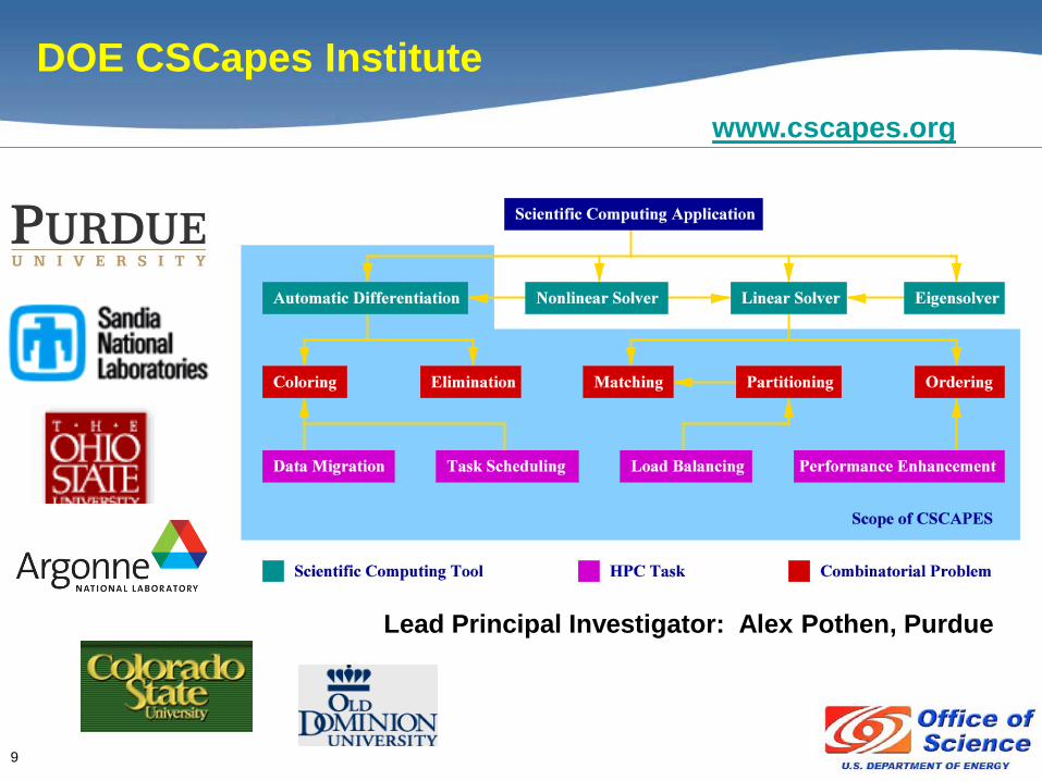
9

Lead Principal Investigator: Alex Pothen, Purdue

www.cscapes.org

DOE CSCapes Institute

http://www.cscapes.org/�

10

A Brief Tour of Applications

11

• Goals: balance load, reduce data movement

• Approaches: geometric, spectral, multilevel

• Geometric meshes are easier than general sparse structures!

• Graphs => hypergraphs, more detailed models

• Partitioning in parallel: how to bootstrap?

Partitioning data for parallel computation

Image courtesy of Mark Adams

Image courtesy of Umit Catalyurek

12

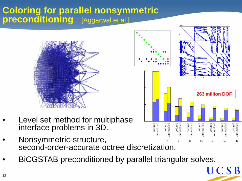
Coloring for parallel nonsymmetric preconditioning [Aggarwal et al.]

• Level set method for multiphase interface problems in 3D.

• Nonsymmetric-structure, second-order-accurate octree discretization.

• BiCGSTAB preconditioned by parallel triangular solves.

263 million DOF

13

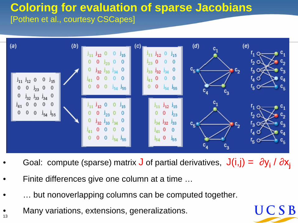
Coloring for evaluation of sparse Jacobians[Pothen et al., courtesy CSCapes]

• Goal: compute (sparse) matrix J of partial derivatives, J(i,j) = ∂yi / ∂xj

• Finite differences give one column at a time …

• … but nonoverlapping columns can be computed together.

• Many variations, extensions, generalizations.

14

• Technique to convert a (complicated) program that computes f(x)into a program that computes ∂fi / ∂xj for all i and j

• Represent a computation as a DAG; vertices are elementary operations

• Label edges with partial derivatives of elementary ops

Function Derivatives

Automatic Differentiation of Programs[Hovland et al., courtesy CSCapes]

15

Automatic Differentiation


• Using the chain rule, eliminate internal vertices

• End up with partial derivatives of outputs with respect to inputs

Derivatives

16





Derivatives

17





Derivatives

18





Derivatives

19


• Used in practice on very large programs => large computational graphs

• Work depends on elimination order; best order is NP-hard

• Checkpointing to trade time for memory; many combinatorial problems

Derivatives

www.autodiff.org

http://www.autodiff.org/�

20

Landscape connectivity modeling[Shah et al.]

• Habitat quality, gene flow, corridor identification, conservation planning

• Pumas in southern California: 12 million nodes, < 1 hour

• Targeting larger problems: Yellowstone-to-Yukon corridor

Figures courtesy of Brad McRae

21

Circuitscape [McRae, Shah]

• Predicting gene flow with resistive networks

• Matlab, Python, and Star-P (parallel) implementations

• Combinatorics:– Initial discrete grid: ideally 100m resolution (for pumas)

– Partition landscape into connected components

– Graph contraction: habitats become nodes in resistive network

• Numerics:– Resistance computations for pairs of habitats in the landscape

– Iterative linear solvers invoked via Star-P: Hypre (PCG+AMG)

22

• How strongly does each transcriptionfactor activate or repress expression of each gene?

• Factorize observation matrix E as P × A

• Topological constraints on A

• Possible nonnegativity constraint on P

• Regularized alternating least squares, etc.

Reverse-engineering genetic transcription[Abdur-Rahim, dePuit, Yuraszeck after Liao etc.]

Liao et al. 2003, PNAS

Observed gene

expression data EUnknown transcription factor

activities P

Microarray ->

DNA makes RNA, regulated by proteins called transcription factors.

Unknown connectivity

strengths A

23

A Few Challenges in Combinatorial Scientific

Computing

24

The Challenge of Architecture

and Algorithms

25

The Architecture & Algorithms Challenge

Oak Ridge / Cray Jaguar> 1.75 PFLOPS

Two Nvidia 8800 GPUs> 1 TFLOPS

Intel 80-core chip> 1 TFLOPS Parallelism is no longer optional…

… in every part of a computation.

26

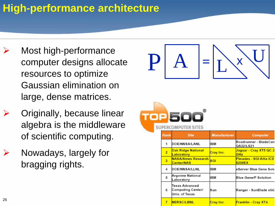
High-performance architecture

Most high-performance computer designs allocate resources to optimize Gaussian elimination on large, dense matrices.

Originally, because linear algebra is the middleware of scientific computing.

Nowadays, largely for bragging rights.

= xP A L U

27

Strongly connected components

• Symmetric permutation to block triangular form

• Diagonal blocks are strong Hall (irreducible / strongly connected)

• Sequential: linear time by depth-first search [Tarjan]

• Parallel: divide & conquer, work and span depend on input[Fleischer, Hendrickson, Pinar]

1 52 4 7 3 61

5

247

36

PAPT G(A)

1 2

3

4 7

6

5

28

Architectural impact on algorithms

Matrix multiplication: C = A * BC = 0;

for i = 1 : n

for j = 1 : n

for k = 1 : n

C(i,j) = C(i,j) + A(i,k) * B(k,j);

O(n3) operations

29

Architectural impact on algorithms

-1

0

1

23

4

5

6

0 1 2 3 4 5

log Problem Size

log

cycles

/flop

T = N4.7

Naïve algorithm is O(N5) time under UMH model.BLAS-3 DGEMM and recursive blocked algorithms are O(N3).

Size 2000 took 5 days

12000 would take1095 years

Diagram from Larry Carter

Naïve 3-loop matrix multiply [Alpern et al., 1992]:

30

A big opportunity exists for computer architecture to influence combinatorial algorithms.

(Maybe even vice versa.)

The architecture & algorithms challenge

31

The Challenge of Primitives

32

An analogy?

As the “middleware” of scientific computing,

linear algebra has suppliedor enabled:

• Mathematical tools

• “Impedance match” to computer operations

• High-level primitives

• High-quality software libraries

• Ways to extract performancefrom computer architecture

• Interactive environments

Computers

Continuousphysical modeling

Linear algebra

33

An analogy?

Computers

Continuousphysical modeling

Linear algebra

Discretestructure analysis

Graph theory

Computers

34

An analogy? Well, we’re not there yet ….

Discretestructure analysis

Graph theory

Computers

√ Mathematical tools

? “Impedance match” to computer operations

? High-level primitives

? High-quality software libs

? Ways to extract performancefrom computer architecture

? Interactive environments

35

Primitives should…

• Supply a common notation to express computations

• Have broad scope but fit into a concise framework

• Allow programming at the appropriate level ofabstraction and granularity

• Scale seamlessly from desktop to supercomputer

• Hide architecture-specific details from users

36

Frameworks for graph primitives

Many possibilities; none completely satisfactory; little work on common frameworks or interoperability.

• Visitor-based, distributed-memory: PBGL• Visitor-based, multithreaded: MTGL• Heterogeneous, tuned kernels: SNAP• Scan-based vectorized: NESL• Map-reduce: lots of visibility• Sparse array-based: Matlab *P-KDT, CBLAS

37

The Case for Sparse Matrices

38

Identification of Primitives

Sparse matrix-matrix multiplication (SpGEMM)

Element-wise operations

x

Matrices on various semirings: (x, +) , (and, or) , (+, min) , …

Sparse matrix-dense vector multiplication

Sparse matrix indexing

x

.*

Sparse array-based primitives

39

Multiple-source breadth-first search

X

1 2

3

4 7

6

5

AT

40

XAT ATX

1 2

3

4 7

6

5


41

• Sparse array representation => space efficient

• Sparse matrix-matrix multiplication => work efficient

• Load balance depends on SpGEMM implementation

XAT ATX

1 2

3

4 7

6

5


42

Why focus on SpGEMM?

• Graph clustering (Markov, peer pressure)• Subgraph / submatrix indexing• Shortest path calculations • Betweenness centrality• Graph contraction• Cycle detection• Multigrid interpolation & restriction• Colored intersection searching• Applying constraints in

finite element computations• Context-free parsing ...

11

11

1 x x

SpGEMM: Sparse Matrix x Sparse Matrix

43

Distributed-memory sparse matrix-matrix multiplication

j

* =i

kk

Cij

Cij += Aik * Bkj

2D block layout Outer product formulation Sequential “hypersparse” kernel

• Scales well to hundreds of processors

• Betweenness centrality benchmark: over 200 MTEPS

• Experiments: TACC Lonestar cluster

Time vs Number of cores -- 1M-vertex RMAT

44

A Parallel Library: Combinatorial BLAS

45

• By analogy to numerical scientific computing. . .

• What should the combinatorial BLAS look like?

The Primitives Challenge

C = A*B

y = A*x

μ = xT y

Basic Linear Algebra Subroutines (BLAS):Speed (MFlops) vs. Matrix Size (n)

46

Applications and Algorithms

Betweenness Centrality (BC)What fraction of shortest paths pass through this node?

Brandes’ algorithm

Software stack for an application of the Combinatorial BLAS

The Combinatorial BLAS: Example of use

47

BC performance in distributed memory

• TEPS = Traversed Edges Per Second

• One page of code using CBLAS

0

50

100

150

200

250

25 36 49 64 81 100

121

144

169

196

225

256

289

324

361

400

441

484

TEPS

sco

reM

illio

ns

Number of Cores

BC performance

Scale 17

Scale 18

Scale 19

Scale 20

RMAT power-law graph,

2Scale vertices, avg degree 8

48

The Education Challenge

How do you teach this stuff?

Where do you go to take courses in

Graph algorithms …

… on massive data sets …

… in the presence of uncertainty …

… analyzed on parallel computers …

… applied to a domain science?

49

Final thoughts

• Combinatorial algorithms are pervasive in scientific computing and will become more so.

• Linear algebra and combinatorics can support each other in computation as well as in theory.

• A big opportunity exists for computer architecture to influence combinatorial algorithms.

• This is a great time to be doing research in combinatorial scientific computing!

combinatorial scientific computing: tutorial, experiences, and

Documents