combined experiment phase i: final report · combined experiment phase i final report c.p....
TRANSCRIPT
October 1992 NREL/TP-257-4655
Combined Experiment Phase I
Final Report C.P. Butterfield W.P. Musial D.A. Simms
National Renewable Energy Laboratory 1617 Cole Boulevard Golden, Colorado 80401-3393 A national laboratory of the U.S. Department of Energy Managed by Midwest Research Institute for the U.S. Department of Energy under contract No. DE-AC36-83CH10093
NREL/TP-257-4655 • UC Category: 261 • DE92000012
Combined Experiment Phase I
Final Report
C.P. Butterfield W.P. Musial D.A. Simms
National Renewable Energy Laboratory 1617 Cole Boulevard Golden, Colorado 80401-3393 A national laboratory of the U.S. Department of Energy Managed by Midwest Research Institute for the U.S. Department of Energy under contract No. DE-AC36-83CH10093
October 1992

NOTICE
This report was prepared as an account of work sponsored by an agency of the United States government. Neither the United States government nor any agency thereof, nor any of their employees, makes any warranty, express or implied, or assumes any legal liability or responsibility for the accuracy, completeness, or usefulness of any information, apparatus, product, or process disclosed, or represents that its use would not infringe privately owned rights. Reference herein to any specific commercial product, process, or service by trade name, trademark, manufacturer, or otherwise does not necessarily constitute or imply its endorsement, recommendation, or favoring by the United States government or any agency thereof. The views and opinions of authors expressed herein do not necessarily state or reflect those of the United States government or any agency thereof.


TP-4655
1.0 Table of Contents
Acknowledgments ill
1.0 Table of Contents . . . . . . . . . . . . . . . . . . . . . . . . . . . . . . . . . . . . . . . . . . . . . . . . . iv
2.0 Introduction . . . . . . . . . . . . . . . . . . . . . . . . . . . . . . . . . . . . . . . . . . . . . . . . . . . . . 1
3.0 Background ~ . . . . . . . . . . . . . . . . . . . . . . . . . . . 2
4.0 Test Setup . . . . . . . . . . . . . . . . . . . . . . . . . . . . . . . . . . . . . . . . . . . . . . . . . . . . . . 3
4.14.24.3
Test Site .Test Turbine . . . . . . . . . . . ~ . . . . . . . . . . . . . . . . . . . . . . . . . . . . . . . . . . .MET Towers .
335
5.0 Instrumentation . 6
5.1 Pressure Measurements '. . . . 65.1.1 Pressure Taps 65.1.2 Pressure Transducer . . . . . . . . . . . . . . . . . . . . . . . . . . . . . . . . . . . . 85.1.3 Pressure System Controller '. . . . 85.1.4 Centrifugal Force Correction . . . . . . . . . . . . . . . . . . . . . . . . . . . . . . 12
5.2 Angle-of-Attack (AOA) Transducer . . . .. . . . . . . . . . . . . . . . . . . . . . . . . . . 125.3 Strain Gages . . . . . . . . . . . . . . . . . . . . . . . . . . . . . . . . . . . . . . . . . . . . . . . 165.4 Anemometers ; . . . . . . . . . . . . . . . . . . . . . . . . . . . . . . . . 185.5 Video Equipment 19
5.5.1 Cameras... . . . . . . . . . . . . . . . . . . . . . . . . . . . . . . . . . . . . . . . . . 195.5.2 Tufts.............................................. 195.5.3 Lighting............................................ 19
5.6 Miscellaneous Transducers . . . . . . . . . . . . . . . . . . . . . . . . . . . . . . . . . . . . . 20
6.0 Data Acquisition and Reduction Systems . . . . . . . . . . . . . . . . . . . . . . . . . . . . . . . . . 21
6.1 Combined Experiment PCM Systems 236.2 NREL PC-Based PCM Data Reduction System Hardware 26
6.2.1 Objectives of PC..PCM System Development 266.2.2 PC-PCM Decoding System Hardware 276.2.3 PC-PCM Decoding System Software 276.2.4 Data Flow in the Computer . . . . . . . . . . . . . . . . . . . . . . . . . . . . . . . 296.2.5 Data Capture Performance Estimates 29
6.2.6 Architecture of PCM Decoder Board 316.3 NREL PC-PCM Data Reduction System "Quick-Look" .
Software . . . . . . . . . . . . . . . . . . . . . . . . . . . . . . . . . . . . . . . . . . . . . . . . . . 336.3.1 Overview of the Quick-Look Program 33
iv

TP-4655
1.0 Table of Contents (continued)
603.2 Limitation of PC-Based Data Processing 346.3.3 Interfacing a PC to the PCM Data Streams . . . . . . . . . . . . . . . . . . . . 356.3.4 Contiguous Data Acquistion 366.3.5 Real-T1Dle Data Monitoring 366.3.6 Data Monitoring Features. . . . . . . . . . . . . . . . . . . . . . . . . . . . . . . . 396.3.7 Factors Affecting Data Monitor Rates 396.3.8 Data Base of PCM Stream Configuration. . . . . . . . . . . . . . . . . . . . . 406.3.9 Data Base of Channel Parameters 406.3.10 Derived Channel Data Base 416.3.11 Rapid Multi-Channel CalibrationCapability 416.3.12 Event Log File 426.3.13 Quick Review of RecordedData. . . . . . . . . . . . . . . . . . . . . . . . . . . 42
6.4 CombinedExperiment Data Processing 426.4.1 Measurement Accuracy . . . . . . . . . . . . . . . . . . . . . . . . . . . . . . . . . . 436.4.2 Features of the Custom Data Calibration System ~ . . . . . . . . . . 446.4.3 CombinedExperiment CalibrationSequences 456.4.4 Field Data Recording and Processing Requirements. . . . . . . . . . . . . .. 476.4.5 Comprehensive Data Postprocessing . . . . . . . . . . . . . . . . . . . . . . . . . 496.4.6 Dynamic Effects 50
7.0 Wind Tunnel Testing 52
7.1 DEIR Tunnel Tests. . . . . . . . . . . . . . . . . . . . . . . . . . . . . . . . . . . . . . . . . 527.2 Ohio State University (OSU) Wind Tunnel Tests 52
7.2.1 Steady Tests 537.2.2 Unsteady Aerodynamics Tests. . . . . . . . . . . . . . . . . . . . . . . . . . . . . 537.2.3 Rough Airfoil Performance . . . . . . . . . . . . . . . . . . . . . . . . . . . . . . . 54
7.3 Colorado State University Wind Tunnel. . . . . . . . . . . . . . . . . . . . . . . . . . . . 547.3.1 Wind Tunnel Test Setup. . . . . . . . . . . . . . . . . . . . . . . . . . . . . . . . . 547.3.2 Data Analysis 577.3.3 Wind Tunnel Results 57
8.0 Rough Airfoil Performance Tests . 60
8.1 Background. . . . . . . . . . . . . . . . . . . . . . . . . . . . . . . . . . . . . . . . . . . . . . . 608.2 Roughness Description . . . . . . . . . . . . . . . . . . . . . . . . . . . . . . . . . . . . . . . . 618.3 Roughness Testing 628.4 Rough Performance Results 628.5 Rough S809 Airfoil Characteristics 648.6 Wind Tunnel and Rotating Comparisons of Rough Airfoil Data 68
9.0 References \ 72
v
·TP-4655
1.0 Table of Contents (con~luded)
Appendices
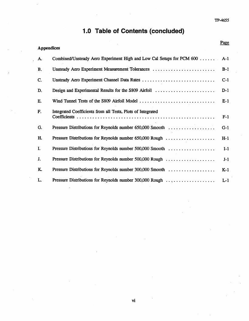
A. CombinedlUnsteady Aero Experiment High and Low Cal Setups for PCM 600 . . . . . . A-I
B. Unsteady Aero Experiment Measurement Tolerances B-1
C. Unsteady Aero Experiment Channel Data Rates . . . . . . . . . . . . . . . . . . . . . . . . . . . . C-l
D. Design and Experimental Results for the S809 Airfoil D-l
E. Wind Tunnel Tests of the S809 Airfoil Model . . . . . . . . . . . . . . . . . . . . . . . . . . . . . E-l
F. Integrated Coefficients from all Tests, Plots of IntegratedCoefficients D • D • • • F-l
G. Pressure Distributions for Reynolds number 650,000 Smooth G-l
H. Pressure Distributions for Reynolds number 650,000 Rough .........•......... H-l
I. Pressure Distributions for Reynolds number 500,000 Smooth 1-1
J. Pressure Distributions for Reynolds number 500,000 Rough J-l
K. Pressure Distributions for Reynolds number 300,000 Smooth K-l
L. Pressure Distributions for Reynolds number 300,000 Rough
vi
. . ':; . L-l

TP-4655
1.1 List of Figures
4-1 Test turbine description . . . . . . . . . . . . . . . . . . . . . . . . . . . . . . . . . . . . . . . . . . . . . . . . 34-2 Test turbine nacelle layout 44-3 Vertical plane array layout 5
5-1 Blade layout . . . . . . . . . . . . . . . . . . . . . . . . . . . . . . . . . . . . . . . . . . . . . . . . . . . . . . . . 65-2 Typical pressure tap frequency response
(.065" In tube, 20" length) 75-3 Typical pressure-tap frequency content
(4% chord, 63% span) 85-4 Transducer installation in blade 95-5 Pressure system controllerblock diagram 105-6 Pressure system controller-pneumatic controls schematic . . . . . . . . . . . . . . . . . . . . .. 115-7 Local flow-angle transducer. . . . . . . . . . . . . . . . . . . . . . . . . . . . . . . . . . . . . . . . . .. 135-8 Upwash effect and terminology 145-9 Wind tunnel calibrationof the local flow-angle sensor 155-10 Dynamic response test of the flow-angle sensor (Reynolds number =10') . . . . . . . . . .. 155-11 lift characteristics at deep stall 165-12 Instrumented blade strain gage - locations and bridge configurations 175-13 Vertical plane array layout. . . . . . . . . . . . . . . . . . . . . . . . . . . . . . . . . . • . . . . . . . .. 18
6-1 CombinedexperimentPCM streams 226-2 Full PCM data reduction and processing 246-3 Data flow in the PC 306-4 Decoder board bit detector . . . . . . . . . . . . . . . . . . . . . . . . . . . . . . . . . . . . . . . . . . .. 326-5 Decoder board frame synchronizer 326-6 PC interface and control 336-7 Quick-look program data flow 386-8 Combined experiment phase II data processing plan . . . . . . . . . . . . . . . . . . . . . . . . .. 51
7-1 Wind tunnel data comparison. . . . . . . . . . . . . . . . . . . . . . . . . . . . . . . . . . . . . . . . .. 537-2 Colorado State University environmental wind tunnel. . . . . . . . . . . . . . . . . . . . . . . .. 557-3 Velocity profile of test section for CSU wind tunnel. . . . . . . . . . . . . . . . . . . . . . . . .. 567-4 Turbulence measurements in test section of CSU wind tunnel 567-5 Reynolds number effects on S809 airfoil and comparison airfoils. . . . . . . . . . . . . .. 587-6 lift and drag results for the S809 airfofl in the CSU wind tunnel. . . . . . . . . . . . . . . .. 59
8-1 60-kilowatt HAWT performance . . . . . . . . . . . . . . . . . . . . . . . . . . . . . . . . . . . . . • .. 608-2 Roughness distribution on leading edges of test turbine blades. . . . . . . . . . . . . . . . . .. 628-3 Combined experiment wind turbine performance 638-4 Normalized power output-s-combined experiment '. . .. 648-5 S809 OSU wind tunnel data . . . . . . . . . . . . . . . . . . . . . . . . . . . . . . . . . . . . . . . . . .. 658-6 Comparison of rough and smooth CL data from rotating and
nonrotating airfoil tests .........................................•.... .66
vii

TP-4655
1.1 List of Figures (concluded)
8-7 0 Change in CL(mu) caused by NACA standard roughness and airfoil thicknessfor typical wind turbine airfoils 67
8-8 LS(1)0413 smooth and rough airfoil performance 688-9 A comparison of pressure distributions for 110 angle of attack . . . . . . . . . . . . . . . . . .. 698-10 A comparison of pressure distributions for 140 angle of attack. . . . . . . . . . . . . . . . . .. 698-11 A comparison of pressure distributions for 180 angle of attack . . . . . . . . . . . . . . . . . .. 70
viii
TP-4655
1.2 List of Tables
Page
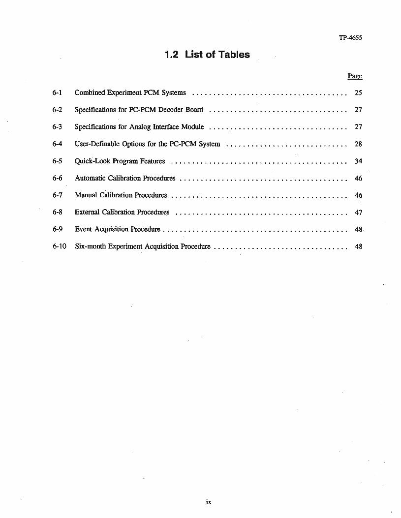
6-1 Combined ExperimentPCM Systems 25
6-2 Specifications for PC-PCM Decoder Board 27
6-3 Specifications for Analog Interface Module 27
6-4 User-Definable Options for the PC-PCM System 28
6-5 Quick-Look Program Features 34
6-6 Automatic Calibration Procedures 46
6-7 Manual Calibration Procedures . . . . . . . . . . . . . . . . . . . . . . . . . . . . . . . . . . . . . . . . .. 46
6-8 External Calibration Procedures 47
6-9 Event Acquisition Procedure . . . . . . . . . . . . . . . . . . . . . . . . . . . . . . . . . . . . . . . . . . .. 48 .
6-10 Six-monthExperimentAcquisition Procedure . . . . . . . . . . . . . . . . . . . . . . . . . . . . . . .. 48
ix

TP-4655
2.0 Introduction
Wind turbine operating experience has shown that current analysis techniques are inadequate when usedto predict peak power and loads on a fixed-pitch wind turbine. Vitema and Corrigan (1981) and TangIer(1983) show evidence of higher-than-predicted power levels on staIl-controlled wind turbines. Becauseperformance and loads are the most important design information needed to achieve more reliable andinexpensive wind turbines, it is important to understand the cause of the discrepancy. The primaryquestion is: How does the wind tunnel airfoil data differ from the airfoil performance on an operatinghorizontal axis wind turbine (HAW1j? The National Renewable Energy Laboratory (NREL) has beenconducting a comprehensive test program focused on answering this question and understanding the basicfluid mechanics of rotating HAWT stall aerodynamics.
The basic approach was to instrument a wind turbine rotor, using an airfoil that was well documented bywind tunnel tests, and measure operating pressure distributions on the rotating blade. Based on theintegrated values of the pressure data, airfoil performance coefficients were obtained, and comparisonswere made between the rotating data and the wind tunnel data. Care was taken to minimize theaerodynamic and geometric differences between the rotating and the wind tunnel models. Models weremade in the same molds, and the same instruments were used for both the rotating and wind tunnel cases.
This is the first of two reports describing the Combined Experiment Program and its results. This Phase Ireport covers background information such as test setup and instrumentation. .It also includes wind tunneltest results and roughness testing. The Phase II report concentrates on the aerodynamic pressure testresults. Average and unsteady aerodynamic measurements are presented. These reports were written fortwo reasons: The first is to disseminate basic aerodynamic data that will be useful for code validation andwind turbine design information. The second is to provide a current orientation for researchers using thedata or participating in the Combined Experiment Program. These reports provide a comprehensivedescription of results to date and a description of how the experiment operates.
' .
1

TP-4655
3.0 Background
The Combined Experiment was planned and carried out over a period of four years. It was the mostcomprehensive wind turbine test program ever attempted, with more than 200 signals simultaneouslymeasured and recorded. The test program was divided into two phases: Phase I planning began in spring1987. Phase II began following the completion of the Phase I tests in spring 1989. Many configurationsof instrumentation were considered during each phase of testing as lessons were learned and instrumentswere improved. Although the instruments were continually upgraded, the major configuration change
. between Phase I and Phase II was the extent of the pressure measurements. The instrumented blade forPhase I had only one span-wise radial station of pressure taps (32 taps) at 80% radius, but the Phase IIblade had four radial stations of pressure taps at radial positions ranging from 30% radius to 80% as wellas six intermediate radial stations of taps located between the primary stations. A new instrumented bladewas fabricated for both Phases I and II. The major instrumentation configuration changes that were madebetween Phases I and II were as follows:
• A thermal drift problem in the Phase I strain gages was corrected with more careful matching ofthe gage and blade thermal expansion properties. .
• A second root-mounted video camera was added to the instrumented blade for Phase II and waspointed toward the tip of the blade. This camera could view the entire blade from one position.
• The R. M. Young U-V-W fixed-axis anemometers on the vertical plane array (VPA), in Phase I,were replaced by prop-vane anemometers.
• Two bi-vane anemometers were added at hub height on the north and south sides of the VPA.
• The sonic anemometer and the hot-film anemometers on the local meteorological tower were notoperating during Phase II.
• In Phase II, a Honeywell 16-channel tape recorder replaced a Sabre-80 14-channel tape recorder.The Honeywell recorder had a higher bandwidth than the Sabre and allowed the tape to be playedslower; therefore, more data per tape were recorded.
Phase I testing was conducted between July 1988 and May 1989. Many of the fifty-five 30-min analogtapes that were recorded were not usable because of various instrumentation problems, but there wereenough good-quality records to establish a baseline data set The Phase I tests were necessary to refine·the details of the instrumentation and data acquisition system to gain a preliminary understanding of howto interpret the pressure measurements and process the data. The Phase I report will cover the test setup.instrumentation, wind tunnel tests, and airfoil roughness testing. Much of the Phase II success can beattributed to the Phase I experience.
Most of the datapresented came from the more comprehensive Phase II data sets and will be presentedin the Phase II report This report will cover the wind turbine test results, including:
• Bin averaged aerodynamic coefficients dataintegrated from pressure distributions
• Bin averaged blade load data
• Unsteady aerodynamic data.
2

TP-4655
4.0 Test Setup
4.1 Test Site
The test site where all the atmospheric testing was conducted is located at the NREL Wind Energy TestCenter at the Rocky Flats Plant 10 miles north of Golden, Colorado. Winter winds are dominant at thissite from a prevailing direction of 292 deg. The local terrainis flat" withgrassyvegetation extending over.1/2' mile upwind. However, the site sits only a few miles from the opening of Eldorado Canyon at thebase of theRocky Mountains, which are located directly upwind. The wind turbinewas unobstructed byother structures or wind turbines. A layout of the wind site and test turbine is given in Simms andButterfield (1990).
4.2 Test Turbine
The Combined Experiment TestTurbinewas a modified Grumman WindStream33. It was a 10-m-diam.,three-bladed, downwind, free-yaw turbine equipped with full span pitch capability that is manuallycontrolled during the testing to provide fixed-pitch (stall-eontrolled) operation at any pitch angle desired.The rotational speed of the rotor was a constant72 RPM. The turbine was supported on a guyed-poletower. It was equipped with a hingedbase and gin pole to allowit to be tilted down easily. An electricwinchwas used to lower and raise the system duringinstallation. A base-controlled yaw lock was addedto allowlocked yaw operation at arbitrary yawpositions from the ground 'This yawretentionsystemhada strain-gaged link to measure yaw moments. Also added was a mechanical caliper brake' system thatcould be operatedmanually from the control shed The specifications for this wind turbine are showninFigure 4-1. A schematic of the turbine's nacelle is shown in Figure 4-2.
10 Meter diameter20 Kilowatt72 RPMConstant chordZero twist5809 airfoil
. Pitch controlDown wind
Camera boom
'Ughts
-Test blade
Angle of attack probe -~~-l-l
Total pressure probe ---lI--t-----,
Tower--
Figure 4-1. Test turbine description
3

TP-4655
1 - Generator2 - Disc brake3 • H.S. shaft4 - Pitch cont actuator5· Swivel6· Gearbox7 - Pillow block bearing8· Cowling9 - Rotor shaft
10 • Fig block bearing11 - Tlirust bearing12 - Vertical shaft13 - Tower14 • Strongback15 - Torque link16 - Redundant pitch cont actuator17 - Redundant pitch actuator crank
Figure 4-2. Test turbine nacelle layout
The new blade was the most significant configuration change. The original .blade platform wasmaintained, but the NREL S809 airfoil replaced the original Grumman airfoil. The S809 airfoil wasdeveloped by Airfoils, Inc., under contract to NREL (Simms and Butterfield, 1990). The primary reasonthis airfoil was chosen was that it had a well-documented wind tunnel data base that includes pressuredistributions, separation boundary locations, drag data, and flow-visualization data.
The blades had a constant .45-m (I8-in.) chord with zero twist. The blade material was a fiberglass/epoxycomposite. The blades were designed to be stiff to limit aero-elastic blade deflections. The dynamiccharacteristics of the blade were tailored to avoid coalescence of rotor harmonics with flap-wise, edgewise, and torsional natural frequencies. To minimize the possibility of aero-elastic instabilities, the massand elastic axes were aligned with the aerodynamic axis. The instrumented blade was painted black tocontrast with the white tufts that were used for flow visualization.
Some of the advantages of this turbine were:
• The rigid, three-bladed rotor reduced the amount of out-of-plane blade motion and minimizedaero-elastic effects.
4
TP-4655
• The constant-chord, zero-twist blade reduced the effects of blade geometry on stalled flow.
• The downwind rotor configuration allowed a boom-mounted camera to view tufts on the lowpress,ure side of the blade withoutobstructions.
• The simplicity, small size, and high availability of parts made test modifications such as towertilting, transducer mounting, and control system changes easy and inexpensive.
." - The manual pitch control system allowed stall-controlled operation at any pitch angle.
4.3 MET Towers
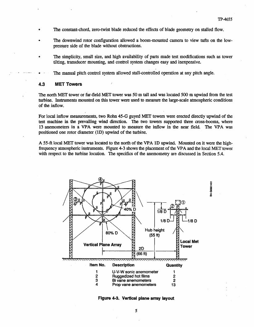
The north :MET tower or far-field :MET tower was 50 m tall and was located 500 m upwindfrom the testturbine. Instruments mounted on this tower were used to measure the large-scale atmospheric conditionsofthe inflow.
For local inflow measurements, two Rohn 45-0 guyed MET towers were erected directlyupwind of thetest machine in the prevailing wind direction. The two towers supported three cross-booms, where13 anemometers in a VPA were mounted to measure the inflow in the near field The VPA waspositioned one rotor diameter (ID) upwind of the turbine.
A 55-ft local MET tower was locatedto the north of the VPA ID upwind Mounted on it were the highfrequency atmospheric instruments. Figure4-3 showsthe placement of the VPA andthe local METtowerwith respect to the turbine location. The specifics of the anemometry are discussed in Section5.4.
"Hub height(55 ft)
Item No. Description"
1 U-V-Wsonic anemometer2 Ruggedized hot films3 Bi vane anemometers4 Propvane anemometers
1/80
Local MetTower
Quantity
122
13
Figure 4-3. Vertical plane array layout
5

TP-4655
5.0 Instrumentation
5.1 Pressure Measurements
5.1.1 Pressure Taps
Blade surface pressures were the most important and the most difficult measurements to make. Theaccuracy of the aerodynamic performance coefficients was dependent on the individual pressure tapmeasurements because each coefficient is the integrated value of the measured pressure distribution at thatradial station. The measurement approach was to install small pressure taps in the surface of the bladeskin. Each opening was mounted flush to the airfoil surface and was 0.040 in. in diameter. The flushprofile was necessary to prevent the taps themselves from disturbing the flow. Stainless steel tubes, eachless than 0.5 m in length, were installed inside the blade's skin during manufacturing to carry surfacepressures to the pressure transducer. For Phase I testing, 32 ressure taps were located at 80% of fullblade span, where the Reynolds number is approximately 10. In Phase II, three more stations wereadded: one at 63%R, one at 47%R, and one at 30%R. The taps were aligned along the chord (instead ofbeing staggered) so that span-wise variations in pressure distributions would not distort measured"chordwise distributions. The chord-wise spacing of the pressure taps is shown in Figure 5-1.
,~l<:-~.'I " ! ! , ! ! , ! ! I Io 10 20 30 40 50 60 70 80 90 100
% Chord (18-in. chord)
100
90
eo
70
~~60
.5~ 50...gC2 40
~
30
20
10
o
----- Indicates fundistributionof taps
---- Indicates 4%and 36%taps only
Figure 5-1. Blade layout
6
TP-4655
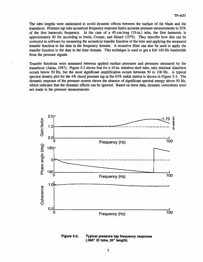
The tube lengths were minimized to avoid dynamic effects between the surface of the blade and thetransducer. Pressure tap tube acoustical frequency response limits accurate pressure measurements to 20%of the first harmonic frequency. In the case of a 45-cm-Iong (I8-in.) tube, the first harmonic isapproximately 80 Hz according to Irwin, Cooper, and Hirard (1979). They describe how this can becorrected in software by measuring the acoustical transfer function of the tube and applying the measuredtransfer function to the data in the frequency domain. A recursive filter can also be used to apply thetransfer function to the data in the time domain. This technique is used to get a full lOO-Hz bandwidthfrom the pressure signals.
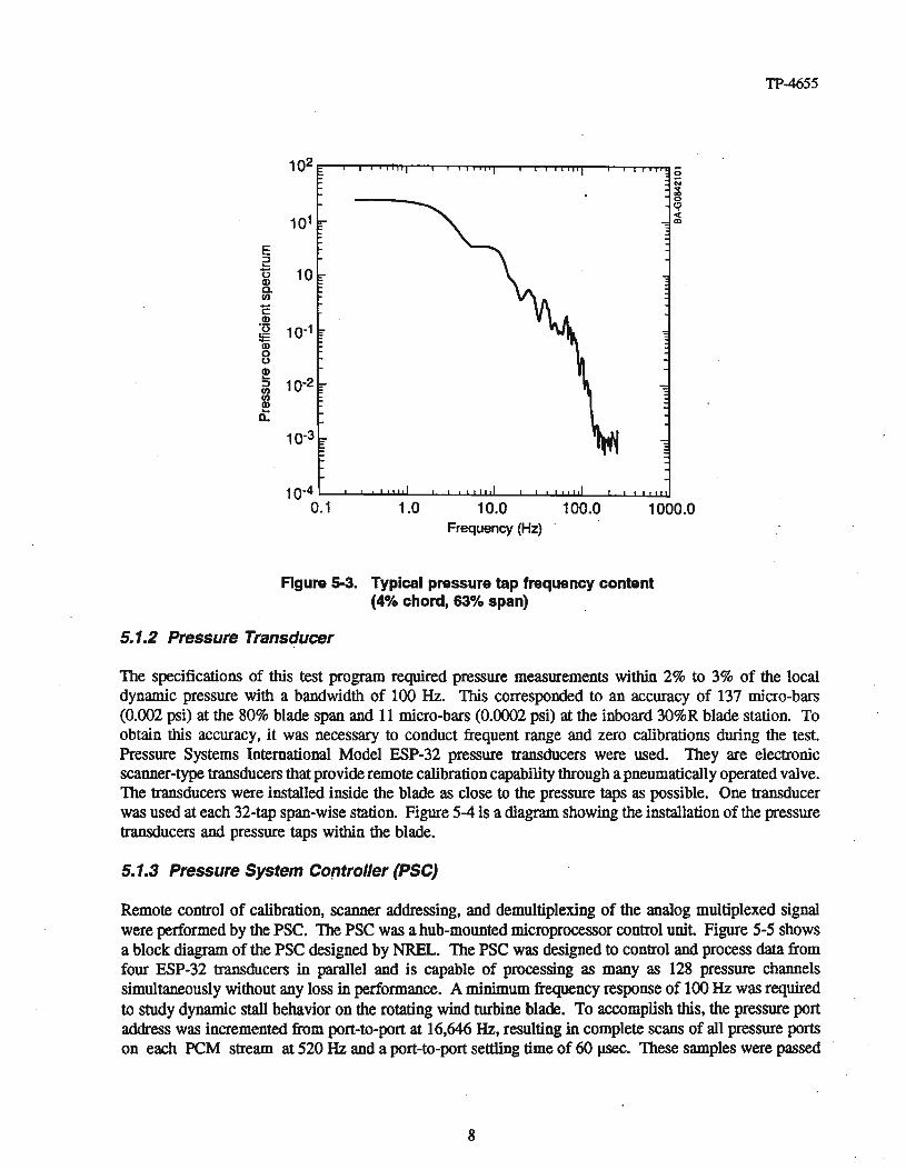
Transfer functions were measured between applied surface pressures and pressures measured by thetransducer (Akins, 1987). Figure 5-2 shows that for a 100in. stainless steel tube, only minimal distortionoccurs below SO Hz, but the most significant amplification occurs between SO to 100Hz. A typicalspectral density plot for the 4% chord pressure tap at the 63% radial station is shown in Figure 5-3. Thedynamic response of the pressure system shows the absence of significant spectral energy above 50 Hz,which indicates that the dynamic effects can be ignored Based on these data, dynamic corrections werenot made to the pressure measurements,
2.0~colB
1.0J---------~~::o=:="=-=~:-=::'= -------------- ~
------------------------~-----
100
100Frequency (Hz)
Frequency (Hz) .
-0>Q)
~Q)
C>c 0enQ)
gJ L-------==================-_L__.J.c 180a.. 0
Q)o .c~Q).!:oo
1.0t=------------- _
100Frequency (Hz)O.O------------------ .....Jo
Figure 5-2. Typical pressure tap frequency response(.065" ID tube, 20'1 length)
7
TP-4655
102
101
E::J...ts 10Q)e-li)
EQ)·u 10-1!i:Q)
8~
10-2::JII)II)Q)...0.
1.0 10.0 100.0Frequency (Hz)
Figure 5-3. Typical pressure tap frequency content(4% chord, 63% span)
5.1.2 Pressure Transducer
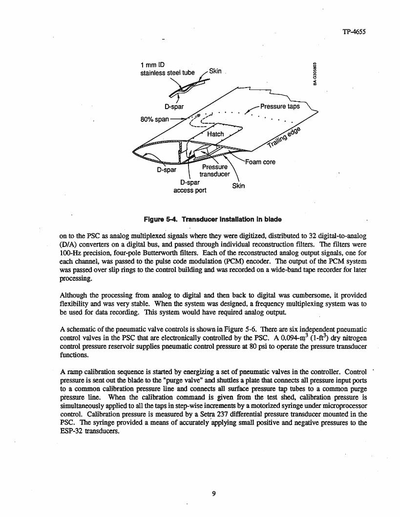
The specifications of this test program required pressure measurements within 2% to 3% of the localdynamic pressure with a bandwidth of 100 Hz. This corresponded to an accuracy of 137 micro-bars(0.002 psi) at the 80% blade span and 11 micro-bars (0.0002 psi) at the inboard30%Rblade station. Toobtain this accuracy. it was necessary to conduct frequent range and zero calibrations during the test.Pressure Systems International Model ESP-32 pressure transducers were used. They are electronicscanner-type transducers thatprovide remote calibration capability throughapneumatically operated valve.The transducers were installedinside the blade as close to the pressure taps as possible. One transducerwasused at each32-tapspan-wise station. Figure5-4 is a diagram showing the installation of the pressuretransducers and pressure taps within the blade.
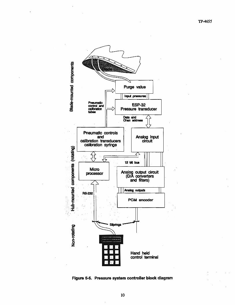
5.1.3 Pressure System Controller (PSC)
Remote control of calibration, scanner addressing, and demultiplexing of the analog multiplexed signalwereperformed by the PSC. ThePSC was a hub-mounted microprocessor control unit Figure 5-5 showsa block diagram of the PSC designed by NREL. The PSC was designed to controland process datafromfour ESP-32 transducers in parallel and is capable of processing as many as 128 pressure channelssimultaneously withoutanyloss in performance. A minimum frequency response of 100Hz wasrequiredto studydynamic stall behavior on the rotating windturbineblade. To accomplish this, the pressure portaddress was incremented from port-to-port at 16,646 Hz, resulting in complete scans of all pressure portson each PCM stream at 520 Hz and a port-to-port settling timeof 60 usee, Thesesamples werepassed
8
1 mm 10stainlessySkin .
D-spar
800/0 span -.-.'"
Pressuretransducer
D-sparaccess port
Skin
C')oCDonoC')
e.(a:I
TP-4655
Figure 5-4. Transducer installation In blade
on to the PSC as analog multiplexed signals where they were digitized, distributed to 32 digital-to-analog(DIA) converters on a digital bus, and passed through individual reconstruction filters, The filters weretOO-Hz precision, four-pole Butterworth filters. Each of the reconstructed analog output signals, one foreach channel, was passed to the pulse code modulation (PCM) encoder. The output of the PCM systemwas passed over slip .rings to the control building and was recorded on a wide-band tape recorder for laterprocessing.
Although the processing from analog to digital and then back to digital was cumbersome, it providedflexibility and was very stable. When the system was designed, a frequency multiplexing system was tobe used for data recording. 'This system would have required analog output
A schematic of the pneumatic valve controls is shown in Figure 5-6. There are six independent pneumaticcontrol valves in the PSC that are electronically controlled by the PSC. A O.094-~3 (l-ff) dry nitrogencontrol pressure reservoir supplies pneumatic control pressure at 80 psi to operate the pressure transducerfunctions.
A ramp calibration sequence is started by energizing a set of pneumatic valves in the controller. Control .pressure is sent out the blade to the "purge valve" and shuttles a plate that connects all pressure input portsto a common calibration pressure line and connects all surface pressure tap tubes to a common purgepressure line. When the calibration command is given from the test shed, calibration pressure issimultaneously applied to all the taps in step-wise increments by a motorized syringe under microprocessorcontrol. Calibration pressure is measured by a Setra 237 differential pressure transducer mounted in thePSC. The syringe provided.a means of accurately 'applying small positive and negative pressures to theESP-32 transducers.
9


TP-4655
If desired, a "purge" command could be given. For this option, a set of valves is energized that sendscontrolpressureto a pneumatically controlled purge valve that is mountednext to the ESP-32. When thepurge valve receives control pressure, all the pressure taps are connected to a regulated supply of drynitrogenat 5 psi that is exhaustedout all the pressure tap tubes to clear moistureor debris. This featurewas exercised before each test to assure that no blockages were present.
Zero calibration was accomplished by energizing a different set of valves that send pneumatic controlpressure out the blade to the ESP-32 transducer, which connects all input pressures to the referencepressure line. Zero calibrations were initiated every 5 min of testing to track zero drift on all channels.
5.1.4 Centrifugal Force Correction
Establishing a referencepressure for each transducer was non-trivial for transducers located in a rotatingenvironment. The air pressures inside the rotating blade were unpredictable and rapidly fluctuating, soit was not possible to establish a reference pressure at the transducer. Instead, the reference tap of eachESP-32 transducer was connected to a single reference pressure line that was terminated at the hubmounted PSC. This created another problem. Centrifugal forces acting on the column of air in thereference tube change the pressure along the radius of the wind turbine rotor. The actual referencepressure experienced by the transducers was calculatedby using the following equation:
(5-1)
where:
Patm =atmospheric pressurePcf =pressure due to centrifugal force
r =radial distance to transducern = rotor speedp = air density.
Tests were run to verify the accuracy of Eq. 5-1 and confirmed the predicted values to within themeasurement accuracy of the transducer.
5.2 Angle-ot-Attack (AOA) Transducer
The main objective of this test programwas to comparewindtunneldata with rotating blade data. Beforethis could be done, an accurate means of measuring and comparing the ADA on a rotating blade wasneeded. Geometric ADA measurements are fairly easy to make in a wind tunnel where the air flow isprecisely controlled, but on rotor they are much more difficult. To accomplish this, it was necessary tomake measurements of the local inflow in front of the blade.
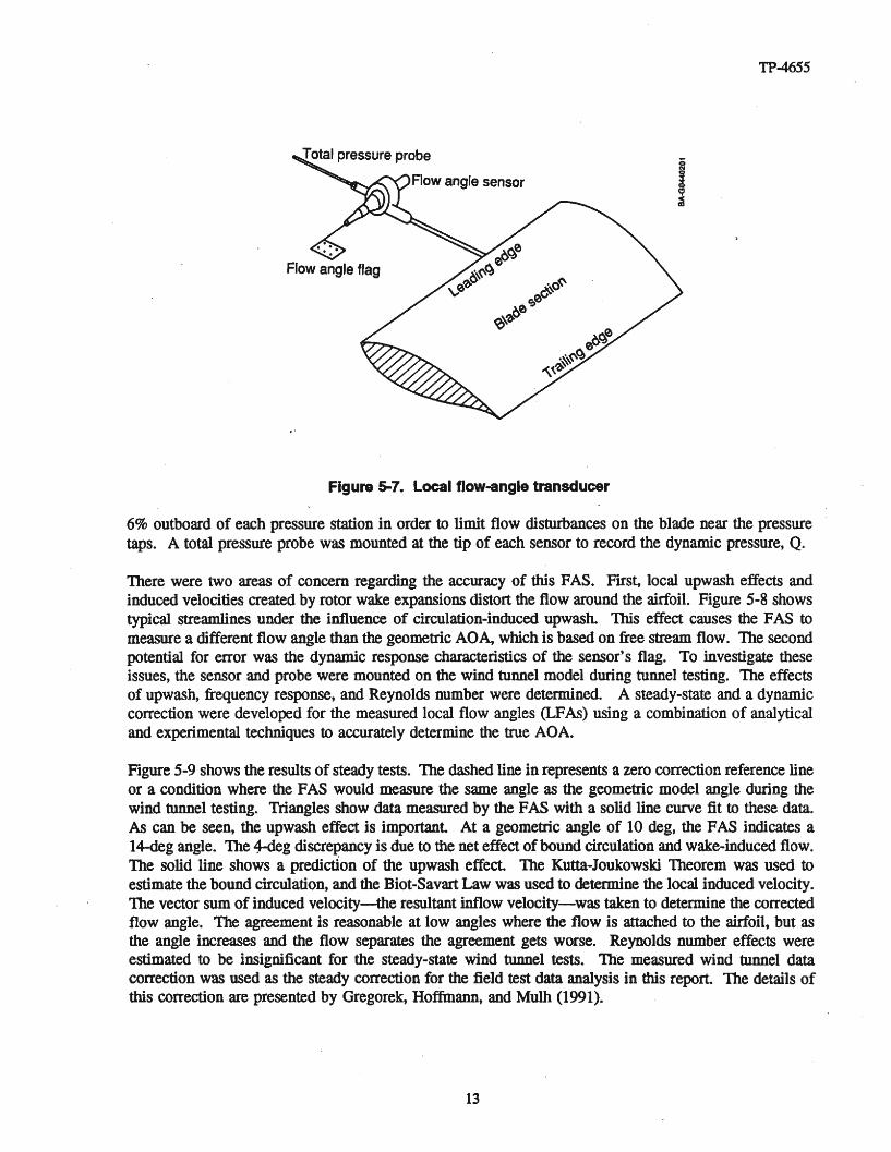
Figure 5-7 shows the flow angle sensor (FAS) that was developed by NREL for this test program.Lenschow (1971)describes earlydevelopment and testingof a similarsensorthat was usedin atmosphericflight testing. The CombinedExperimentFAS used a small, lightweight rigid flag that aligneditself withthe local flow. The flag angle is measured with a commercial rotary positionsensor mountedin a customhousing. The analog signals generated were sent to the hub, multiplexed, and recorded with the othersignals by the dataacquisition system. Flag angles were measured within O.I-deg accuracy. The sensorwas mounted36 cm aheadof the leadingedgeon 5/8-in.-diam. carbontubes. Transducers werepositioned .
12
TP-4655
Total pressure probe
Row angle sensor
Figure 5-7. Local flow-angle transducer
6% outboard of each pressure station in order to limit flow disturbances on the blade near the pressuretaps. A total pressure probe was mounted at the tip of each sensor to record the dynamic pressure, Q.
There were two areas of concern regarding the accuracy of this FAS. FIrSt, local upwash effects andinduced velocities created by rotor wake expansions distort the flow around the airfoil. Figure 5-8 showstypical streamlines under the influence of circulation-induced upwash. This effect causes the FAS tomeasure a different flow angle than the geometric AOA, which is based on free stream flow. The secondpotential for error was the dynamic response characteristics of the sensor's flag. To investigate theseissues, the sensor and probe were mounted on the wind tunnel model during tunnel testing. The effectsof upwash, frequency response, and Reynolds number were determined. A steady-state and a dynamiccorrection were developed for the measured local flow angles (LFAs) using a combination of analyticaland experimental techniques to accurately determine the true ADA.
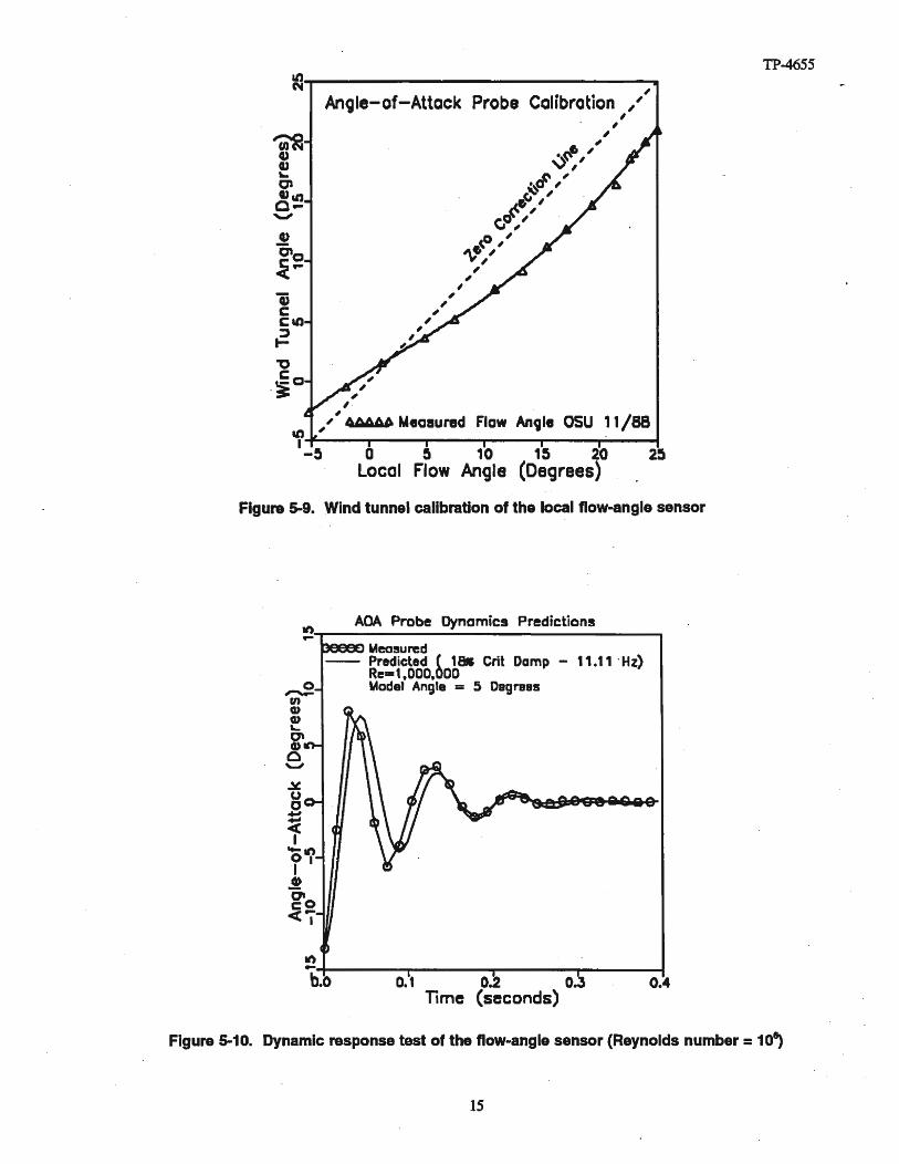
Figure 5-9 shows the results of steady tests. The dashed line in represents a zero correction reference lineor a condition where the FAS would measure the same angle as the geometric model angle during thewind tunnel testing. Triangles show data measured by the FAS with a solid line curve fit to these data.As can be seen, the upwash effect is important At a geometric angle of 10 deg, the FAS indicates a14-deg angle. The 4-deg discrepancy is due to the net effect of bound circulation and wake-induced flow.The solid line shows a prediction of the upwash effect. The Kutta-Joukowski Theorem was used toestimate the bound circulation, and the Biot-Savart Law was used to determine the local induced velocity.The vector sum of induced velocity-the resultant inflow velocity-was taken to determine the correctedflow angle. The agreement is reasonable at low angles where the flow is attached to the airfoil, but asthe angle increases and the flow separates the agreement gets worse. Reynolds number effects wereestimated to be insignificant for the steady-state wind tunnel tests. The measured wind tunnel datacorrection was used as the steady correction for the field test data analysis in this report. The details ofthis correction are presented by Gregorek, Hoffmann, and Mulh (1991).
13

TP-4655
To determine the dynamic response of the FAS, the flag was deflected and released in the wind tunnelat various Reynolds numbers. By recording the decay of the oscillations, a second-order system naturalfrequency and logarithmic damping ratio were determined. Figure 5-10 shows the angular displacementof the flag as the oscillations decay. Also shown are the analytical approximations for each case. Fromthe comparisons, it is clear that the FAS,is 'well damped but not critically damped, and the second-orderdifferential equations model the response well.
There is at least one caution that should be recognized pertaining to the above discussion. It is possiblethat dynamic bound circulation changes could cause local flow field modifications that would. alter thesteady correction shown in Figure 5-9. These effects are unknown at this time. Future dynamic stall windtunnel tests will attempt to address this issue. To investigate this, the FAS will be mounted on a windtunnel model in the tunnel while the model ADA is oscillated at representative frequencies. The effectof the dynamic flow field on upwash will be reflected in a comparison between geometric ADA andmeasured LFA.
Pressure Distributions
Integrated Forces
a • Geometric angle-of-attack
9 - a + localinduced velocity effectCL • Uft coefficientCo. Drag coefficientCN • Normal forcecoefficient
CT· Tangent Force CoefficientCm • Pitching moment coefficient
Figure 5-8. Upwash effectand terminology
14
TP4655
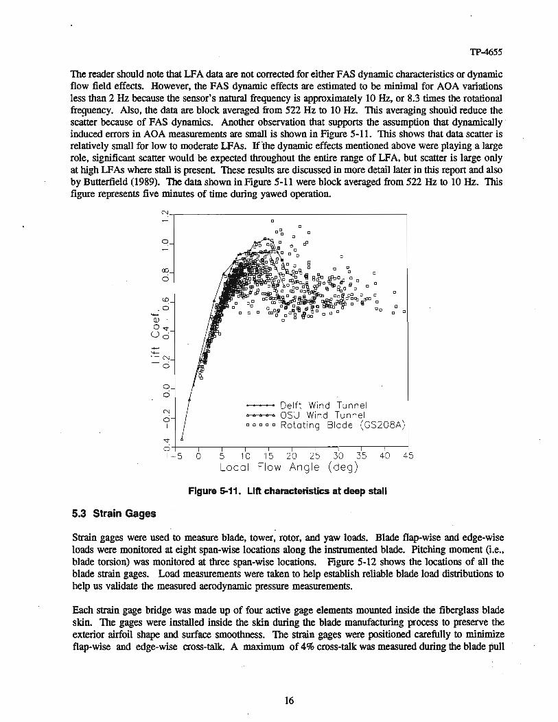
The reader should note that LFA data are not corrected for either FAS dynamic characteristics or dynamicflow field effects. However, the FAS dynamic effects are estimated to be minimal for AOA variationsless than 2 Hz because the sensor's natural frequency is approximately 10 Hz, or 8.3 times the rotationalfrequency, Also, the data are block averaged from 522 Hz to 10 Hz. This averaging should reduce thescatter because of FAS dynamics. Another observation that supports the assumption that dynamicallyinduced errors in AOA measurements are small is shown in Figure 5-11. This shows that data scatter isrelatively small for low to moderate LFAs. If the dynamic effects mentioned above were playing a largerole, significant scatter would be expected throughout the entire range of LFA, but scatter is large onlyat high LFAs where stall is present These results are discussed in more detail later in this report and alsoby Butterfield (1989). The data shown in Figure 5-11 were block averaged from 522 Hz to 10 Hz. Thisfigure represents five minutes of time during yawed operation.
"l
0
co0
<.0,0--(l)o~
U64-'--,- "l-I .
0
00
"l
0I
~
01-5 0
oo
o
c
o
oo 0
Delft Wind Tunnel'" to to to .. OSU Wind Tunnel00000 Rotating Blade (GS208A)
5 10 15 20 25 30 35 40 45Local Flow Angle (deg)
Figure 5-11. Lift characteristics at deep stall
5.3 Strain Gages
Strain gages were used to measure blade, tower, rotor, and yaw loads. Blade flap-wise and edge-wiseloads were monitored at eight span-wise locations along the instrumented blade. Pitching moment (i.e.,blade torsion) was monitored at three span-wise locations. Figure 5-12 shows the locations of all theblade strain gages. Load measurements were taken to help establish reliable blade load distributions tohelp us validate the measured aerodynamic pressure measurements.
Each strain gage bridge was made up of four active gage elements mounted inside the fiberglass bladeskin. The gages were installed inside the skin during the blade manufacturing process to preserve theexterior airfoil shape and surface smoothness. The strain gages were positioned carefully to minimizeflap-wise and edge-wise cross-talk. A maximum of 4% cross-talk was measured during the blade pull
16
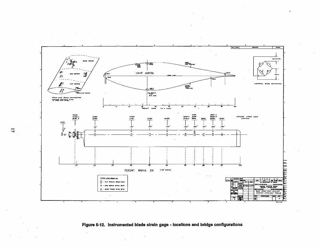
TP-4655
and strain gage calibration tests. These cross-channel interference effects were not considered significant,and corrections were not applied to the data
5.4 Anemometers
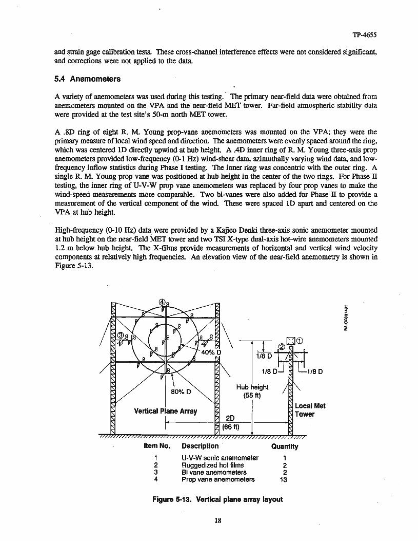
A variety of anemometers was used during this testing. ' The primary near-field data were obtained fromanemometers mounted on the VPA and the near-field .METtower. Far-field atmospheric stability datawere provided at the test site's 50-m north.MET tower.
A .80 ring of eight R. M. Young prop-vane anemometers was mounted on the VPA; they were theprimary measure oflocal wind speed and direction. The anemometers were evenly spaced around the ring,which was centered 10 directly upwind at hub height A 040 inner ring of R. M. Young three-axis propanemometers provided low-frequency (0-1 Hz) wind-shear data, azimuthally varying wind data,and lowfrequency inflow statistics during Phase I testing. The inner ring was concentric with the outer ring. Asingle R. M. Young prop vane was positioned at hub height in the center of the two rings. For Phase IItesting, the inner ring of U-V-W prop vane anemometers was replaced by four prop vanes to make thewind-speed measurements more comparable. Two bi-vanes were also added for Phase II to provide ameasurement of the vertical component of the wind. These were spaced 10 apart and centered on theVPA at hub height
High-frequency (0-10 Hz) data were provided by a Kajieo Denki three-axis sonic anemometer mountedat hub height on the near-field MET tower and two TSI X-type dual-axis hot-wire anemometers mounted1.2 m below hub height The X-films provide measurements of horizontal and vertical wind velocitycomponents at relatively high frequencies. An elevation view of the near-field anemometry is shown inFigure 5-13.
Vertical Plane Array
Hub height(55 ft)
20(66 ft)
1/80
Local MetTower
Item No. Description ·
1 U-V-W sonic anemometer2 Ruggedized hot films3 Bi vane anemometers4 Prop vane anemometers
Quantity
122
13
Figure 5-13. Vertical plane array layout
18

TP-4655
Far-field atmospheric data were recorded from the north MET tower. These data included temperaturegradient, wind shear up to 50 m, relative humidity, and wind directions at four different altitudes. Thesedata combined allowed measurements of atmospheric stability (Richardson number) to be made. Thesedata were multiplexed near the tower base and telemetered to the Combined Experiment test shed wherethey were recorded.
5.5 Video Equipment
5.5.1 Cameras
A lightweight 10-ft boom was designed and mounted to the hub to hold the 10-lb, high-shutter-speedvideo camera. The boom and camera arrangement was designed to be stiff with a system fundamentalfrequency of 10 cycles per revolution (lOP), and the axes of the boom and camera were mass balancedabout the axis of rotation. The lo-ft boom length allowed a view angle of 30 deg at the tip of the bladeand 45 deg at the 66% span. Additional equipment, such as the data acquisition system, the PSC, andlighting for night testing were also mounted on the boom.
For Phase I testing, a NISUS N-2000 video camera was used. A video monitor and recorder in the testshed were used to observe tufts on the low-pressure side of the blade. The camera used a mechanicalshutter to freeze video frames in 1/625 of a second. Thirty video frames were recorded every second toallow one frame to be recorded for every 11 deg of rotor azimuth position. The horizontal resolution ofthis system is limited to approximately 250 lines. One problem with this system was that good angularmeasurements of the tufts were difficult to interpret from the video images. For Phase II, the entire videosystem was upgraded to improve the images of the tufts. The boom-mounted NISUS camera was replacedby acolorPanasonic model WV-CL300. A second camera, aPanasonic WV-BD400 with a 15 to 160 romRainbow G10X16ME zoom lens, was also added to provide another independent view angle along theblade span. 'This camera was mounted on the blade itself and was allowed to pitch with the blade. Thisview provided a full span picture of all the tufts at one time and was instrumental in helping to identifyand match flow patterns with the aerodynamic phenomena observed in the data.
5.5.2 Tufts
Tufts were attached to the surface of the instrumented blade to allow the air flow over the blade to bevisualized. The tufts were made of thin, white, polyester thread measuring approximately 0.25 mm indiameter and 45 rom in length. They were attached to the downwind side of the blade with a small dropof fast drying glue. Tufts were placed in rows spaced 76 rom (3 in.) apart in the blade span-wisedirection. In each row, the tufts were spaced one every 10% of the chord. The tufts on the leading edgeand at 10% chord were intentionally omitted to avoid blade roughness effects that might have been createdby the tufts themselves. The diameter of the tufts was chosen to minimize the effects on the boundarylayer yet maintain good visibility for the video camera. If the tufts were large relative to the boundarylayer thickness, they could cause transition or premature separation. This effect is discussed in more detailby Rae and Pope (1984).
5.5.3 Lighting
Night testing was generally preferred over daytime tests. The black coloring of the blade that was chosento enhance the contrast of the tufts caused differential heating of the blade surfaces during the day. Thisled to a thermal drift problem with the blade strain gages. Also, daylight tended to produce a largeamount of glare and reflections that interfered with the video images. Night testing required lighting tobe added to illuminate the white tufts. Eleven tungsten-halogen 120-V spotlights were placed along thecamera boom and directed at the blade. With this configuration, the video pixel intensity of .a tuft was
19

TP-4655
35 on a gray scale of 0 to 256, and the black background was 10 to 15; the contrast was great enough sothat the tufts couId be seen easily. Unfortunately, there was still not enough light to operate the camerashutter, and moving images were blurred on the video display. In Phase II, the camera resolution wasgreatly improved, and remote control of the iris and focus adjustments were added.
5.6 Miscellaneous Transducers
In addition to the extensive hub-mounted instrumentation, several other measurements were required tocomplete the investigation of this turbine. Strain gages were mounted on the main shaft of the turbineto measure rotor torque and main shaft bending on two axes. Tower bending gages were mounted on twotower bending axes at the point just above the guy wire attachment These gages were oriented tomeasure bending in the direction of the prevailing wind and orthogonal to the prevailing wind Gageswere mounted on the arm of the yaw brake to allow the measurement of yaw moment when the yaw brakewas engaged. Special sensors were developed to measure yaw position (gear-driven potentiometer), pitchangle (gear-driven potentiometer), and rotor azimuth position (Trump Ross 512pulselrevolutionincremental encoder). Generator power was monitored using an Ohio Semitronics, Inc. (OSI) transducerin the test shed.
20
TP-4655
6.0 Data Acquisition and Reduction Systems
To accomplish the objectives of the Combined Experiment requirescollecting data from three majorareas:turbine rotating, turbine non-rotating, and meteorological. In the rotating turbine frame, measurementsare made on the turbine blades, blade attachments, and hub. Typical parameters include strain gagebending moments andtorsion,airfoilsurfacepressuredistributions, totaldynamic pressure, andbladepitchangle. Thesemeasurements providedata to determine blade aerodynamic and structural loads. In the nonrotatingturbineframe, measurements characterize machine performance anddetermine turbineloads. Thisrequires data from the turbine nacelle and tower, such as generator power production; tower bending,azimuth and yaw angles, and rotation speed.
To determine characteristics of the wind at the turbine, meteorological conditions are measured.Anemometers are used to measure near-field horizontal and vertical wind shear. This requires manychannels of wind-speed and wind-direction data from local upwind anemometer arrays. Atmosphericstability measurements are also important in evaluating inflow characteristics. This requires far-fieldatmospheric boundary layer measurements, includinganemometry, temperature, barometric pressure, anddew point
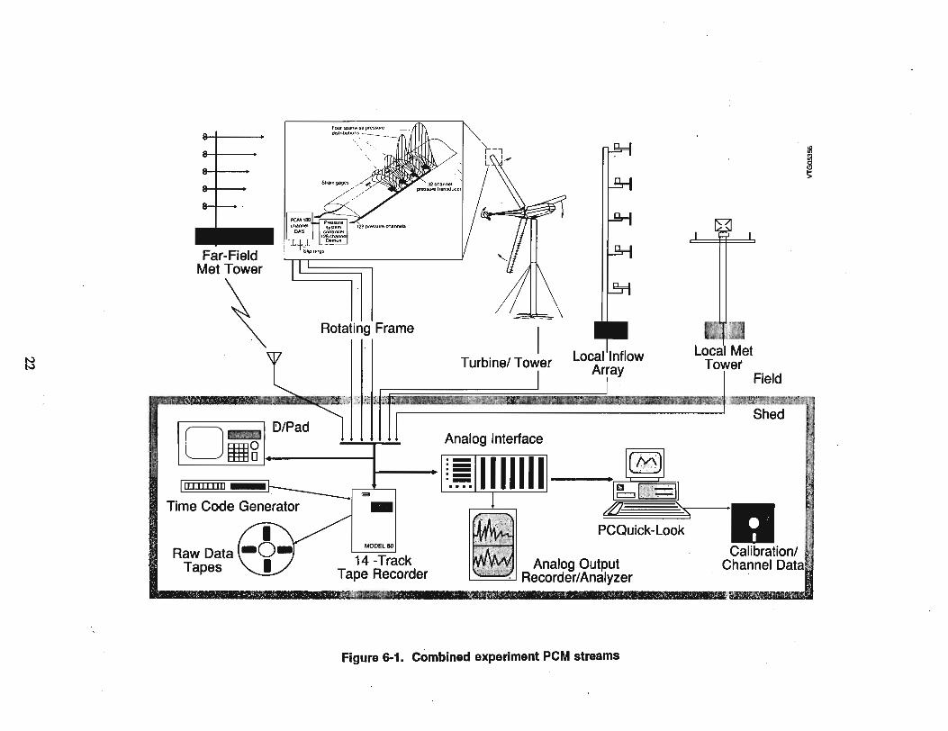
In an effort to increase accuracy, simplify instrumentation, and reduce noise, analog data signals aresampled and encoded into digital PCM streams as close to the measurement source as possible. Thestreams are then telemeteredto a convenient central receiving location and recorded on multi-track tape.Streams are conducted throughslip rings and cablesor transmitted over a radio frequency (RF) link. PCMstream layouts for the Combined Experiment are shown in Figure 6-1 and describedin Section 6.1.
The Combined Experimentuses a customized digital PCM-based hardware system for data acquisition.The system was developed and is used for the following reasons:
• To provide required measurement bandwidth and accuracy, especially from pressure measurementson the rotating blade, and to minimize induced noise and electronic drift in rugged and harshenvironments
• To perform automated multi-channel calibrations that enable essential rapid data verification in thefield
• To generate all required ancillary parameters, provide uncertainty analyses, and allow completecomprehensive data postprocessing.
The system accomplishes these objectives by incorporating military-spec PCM encoders that digitizeanalog signals close to the measurement source and transmit information in digital format to the ground.The system also has built-in microprocessor-controlled calibrationcapabilities and prescribedcalibrationtechniques that were designed to ensure data accuracy.
NREL developed a low-cost PC-based PCM decoding system specifically for use in the CombinedExperiment to facilitate quick PCM data analysis. We were severely limited in our ability to decodemultiple PCM streams for quick-look data processing and display in the field. There were no costeffectivecommercial systemsavailable thatprovidedthe requiredcapabilities. We neededmultiple-streamdecoding, derivation of parameters from multiple channels (across PCM streams), graphic display, datastorage, and a means to rapidly update calibration coefficients. We also needed the ability to monitorlong-termmeteorological conditions for evaluating currenttest status. Thesefieldcapabilities are essential
21

TP-4655
because debugging using laboratory-based postprocessing is inefficient and impractical. We thereforedeveloped PC-bas~ PCM decoding hardware (Simms and Butterfield, 1990) and wrotea custom"QuickLook" PCM data management software program (Simms, 1990). These are described in Sections 6.2and 6.3.
After initial field-based verification, PCM data streams from the Combined Experiment recorded onwide-band tape are extensively postprocessed in the laboratory. Many phases of comprehensive numbercrunching are necessary to produce the final required data sets to prescribed accuracy limits. These aredescribed in Section 6.4. The basic processes involved are as follows:
• Use the PC-based Quick-Look system to produce valid calibration coefficients for all measuredchannels.
• Use a custom laboratory-based telemetry data reduction system called the EXPRT PCMDecommutation System (Fairchild Weston, 1985) to merge the PCM streaminto a continuous timeseries.
• Use ·various UNIX-based computer systems and custom software to perform engineering. unitconversions, deriveancillary parameters, generate spectra, provide digitalfiltering, generate statistics,and maintain a data base of all data records.
The data postprocessing path is shownin Figure 6-2. Along the way, there are also many data integritychecks. Final data records contain 239 channels at 520 samples per second. They are stored in 5-minlong engineering unit records, each requiring 150 Mbytes of disk storage space. We use an erasableoptical disk system and a PC-baseddatabase programto managethe current5-h, 18-Gbyte data set Wehave also developed a digital data processing systemto filter datasets from l00-Hz to 40-, 10-, and I-Hzbandwidth and generatepower spectrain various frequency ranges. These are used to ensuredata qualityand facilitate subsequent data analyses.
6.1 Combined Experiment PCM Systems
PCM-encoded telemetry data systems provide highly accurate measurements over a wide dynamic rangewith low noise (Strock, 1983). These systems are ideal for collecting data related to the study of windturbines, especially in the Combined Experiment, whichrequires accurate multiple-channel measurementstaken from a variety of different locations. PCM systems consistof two basic components:
• Encoders to convert incoming analog signals into digital PCM values
• Decoders to decommutate the PCM values into data that can be computer processed.
Six PCM streams are used for datacollection. Three streams are recordedin the rotating frame, two fromlocal inflowand the turbine/tower, and one from far-field meteorology. Characteristics of the streams aresummarized in Table 6-1.
23


TP-4655
Table 6-1. Combined Experiment PCM Systems
Bit Sample Number Sample PCMPCM rate rate of interval source
# (Kbitls) (Hz) channels (msec) location
1 7.5 34.72 16 28.8 Far MET2 15 69.44 16 14.4 Inflow3 60 277.78 16 3.6 InflowfTurbine4 400 520.83 62 1.92 Rotor8 400 520.83 62 1.92 Rotor9 400 520.83 62 1.92 Rotor
The six PCM streams bring data from multiple sources in the field to a central location where they arecollected, verified to ensure accuracy, and recorded to provide for subsequent laboratory-based processingand analysis. The system layout is shown in Figure 5-1 and is described in detail in Butterfield andNelson (1990) and Butterfield, Jenks, Simms, and Musial (1990). All measurement transducers providelinear output volumes that are conditioned as specified in Appendix A and then input directly to PCM
. encoders. The signal conditioning/PCM encoding for streams 1, 2, and 3 each use a Fairchild-Weston16-channel EMR 600 PCM Data Acquisition System that operates at various bit rates depending on databandwidth requirements. The EMR 600 systems have a specified accuracy of 0.2% of full scale over theoperating temperature range -50° to 120 OF. For PCM 1, the EMR. 600 system is located in the datashedat site 1.1. Its PCM stream is telemetered to site 3.3 over an RF link. The EMR. 600 systems for PCMstreams 2 and 3 are located in the data shed at site 3.3. Analog signals for these two systems areconducted over cables from local transducers on the VPA and from the tower and nacelle. All theEMR 600 systems are in locations that offer a conditioned environment to minimize temperature-induceddrift effects. .
Streams 4, 8, and 9 each use a customized signal conditioning system coupled with three Lora! 61062-channel PCM encoders. The Lora! 610s are specified as having full-scale accuracy of 0.4% over theoperating temperature range of -400 to 185 OF. - This is for digitizing and PCM encoding only. Signalconditioning accuracy varies depending on measurement type, as described below. These systems are alllocated on the wind turbine in the hub-mounted rotor package. The three PCM signals from the rotatingframe are conducted through slip rings and run down the tower to the data shed. All operate at400 Kbitlsec, which provides a datasample rate of520.83 Hz on all 186 channels. The six PCM encodersprovide the capability to measure 234 channels. Of these, 185 are currently considered active andnecessary for the Unsteady Aero Experiment Deactivated channels are for spare or redundantmeasurements, or they were used in previous phases of experimentation. In addition to the 185 directmeasurements, there are five channels allocated for time and 45 subsequently derived ancillary parameters(i.e., integrated pressure distributions, disk-averaged wind speed, induced aerodynamic forces, etc.).
PCM encoders convert conditioned analog input voltages into digital counts. Overall accuracy is limitedby the number of bits used in the digital code. All channels are sampled with 12-bit resolution thatproduces count values in the range from 0 to 4,095. This limits quantizing errors to .024% of full scale,provides a peak signal-to-noise ratio (SIN) of 83 dB, and defines maximum possible dataaccuracy. Allchannels in the Combined Experiment have been set up so that the required data range occupies as muchof the available quantizing range as possible. Resulting quantizing errors are insignificant when comparedto other sources of error in the data acquisition and processing procedures. .
25

TP-4655
6.2 NREL PC-Based PCM Data Reduction System Hardware
In a single PC, the PCM decoding system provides continuous data acquisition to memory or disk fromup to four streams simultaneously. A variety of software packages can subsequently be used to read andprocess the data. Single-stream real-time datamonitoring is accomplished from a graphic bar chart displayprogram.
The full complement of boards in a PC permits data handling from a maximum of 16 PCM streamscontaining up to 62 channels each. The boards are Inter-Range Instrumentation Group (IRIG) compatibleand are designed for use with standard PCM encoders . The data streams can be accessed by cyclicsampling or simultaneous' acquisition or both. Maximum acquisition rates and data storage capacitydepend on PC hardware.
Optional analog interface modules can be used in conjunction with the PC-PCM decoder boards. Theseprovide digital-to-analog conversion of up to 8 user-selectable channels per PCM stream, or 32 channelstotal. Incorporating the PC-PCM system into small portable computers simplifies remote test monitoringof PCM data. The complete system provides test engineers with the ability to decode PCM data andperform quick-look data analysis in the field.
6.2.1 Objectives of PC-PCM System Development
The NREL PC-PCM system consists ofAT-compatible hardware boards for decoding and combining PCMdata streams and DOS software for control and management of data acquisition. Up to four boards canbe installed in a single PC, providing the capability to combine datafrom four PCM streams direct to diskor memory.
Our main objective was to provide a cost-effective PCM decoding system that could be duplicated at ourmany test sites to maintain consistency among systems. Future plans include development of aninexpensive turn-key data acquisition system that could be used by the wind industry. For many reasonsdescribed below, we decided that a PC-based system was most practical.
We contracted with a local electronics development company (Apex Systems, 1988) to develop thePC-based PCM decoding capability. We wanted a system built on printed circuit boards that could beinstalled in the expansion slots of a PCIAT or compatible computer. The system should include basiccontrol software to initialize and operate the boards. It should also provide a simple user interface toallow easy acquisition and examination of data from different PCM streams.
We specified four PCM input channels for each board, from which one could be software selected to readdata. A maximum of four boards could be installed, which would allow access to 16 PCM streams froma single computer. Multiple boards would permit acquisition from up to four streams simultaneously, andwould tag and interleave multiple incoming data into a contiguous digital time series.
We also specified that databe written directly to PC memory or disk meso This would enable subsequentdata processing and analysis to take advantage of the huge resource of software packages available forPCs, according to user preference. It also would enable easy development of custom packages in themany available software languages. The widespread use of PCs also would permit easy distribution ofa developed data acquisition and processing package to interested users.
26

TP-4655
6.2.2 PC-PCM Decoding System Hardware
The PC-PCMhardware boards support a subset of the IRIG PCM standard, designed to synchronize anddecommutate NRZ or Bi-Phase L PCM streams in the range of 1 to 800 Kbits/sec at 8 to 12 bits/wordand 2 to 64 words/frame. Multiple PCM streams (at various rates) can be combined and interleaved intoa contiguous digitaltime series. Maximum datathroughput depends on characteristics of the PC hardware,such as central processing unit (CPU) rate and disk access speed. We typically do not super-multiplexor subcommutate channels in the .PCM"frames. All channels on a givenPCM encoderare sampled at thesame rate as that required for the highest rate channel. Those channels that do not require the fast rateare anti-alias filtered to a lowerbandwidth and can subsequently be decimated in software. The PC-PCMdecoder board specifications are summarized in Table 6-2.
Table 6-2. Specifications for PC-PCM Decoder Board
Bit rateInput streamsInput polarityInput resistanceCodesBit sync typeInput data format
Words per frameSync words per frame
1-800 Kbits/sec4 (only one processed at a time)Negative or positive> 10 KohmsBi-phase L, NRZPhase-locked loop (PLL)8-12 bits/word, most significant bit(MSB) first
2-64 Oncludingsync)1-3 (maximum 32 bits)
In conjunction with the PCM decoderboards, we developed an analog interfacemodulethat reconstructsanalog output from up to eight channels per stream. The basic intent was to provide the ability to usereal-time analog test instruments such as a spectrum analyzer or a chart recorder. The analog module isan optional part of the system. Specifications are shown in Table 6-3.
Table 6-3. Specifications for Analog Interface Module
Analog outputOutput polarityOutput rangePCM inputStatus lights
8 channels (user selectable via thumb wheels)Unipolar or bipolaro to 10 V, 0 to 20 V, -5 to +5 V, -10 to +10 V4 (only one processed at a time)PLL lock, frame sync, first-in, first-out(FIFO), disabled
6.2.3 PC-PCM Decoding System Software
The PC-PCMhardware boards are controlled by DOS software written in C. Three programs and threeASCIIconfiguration files providebasiccapabilities. Thefirst program, PCMTEST, initializes boardsandcaptures data. The second program, PCMDUMP, reads capturedbinary data files. The third program,PCMBAR, generates a real-time bar chart graphics display. These programs input PCM systemdescriptions from DOS ASCn format data files that are easily accessed and modified by the user. Aconfiguration file (.CFG) contains information describing how PCM hardware boards are configured inthe PC. A stream file (.STM) defines characteristics of each PCM stream. The capture file (.CAP)
27
TP-4655
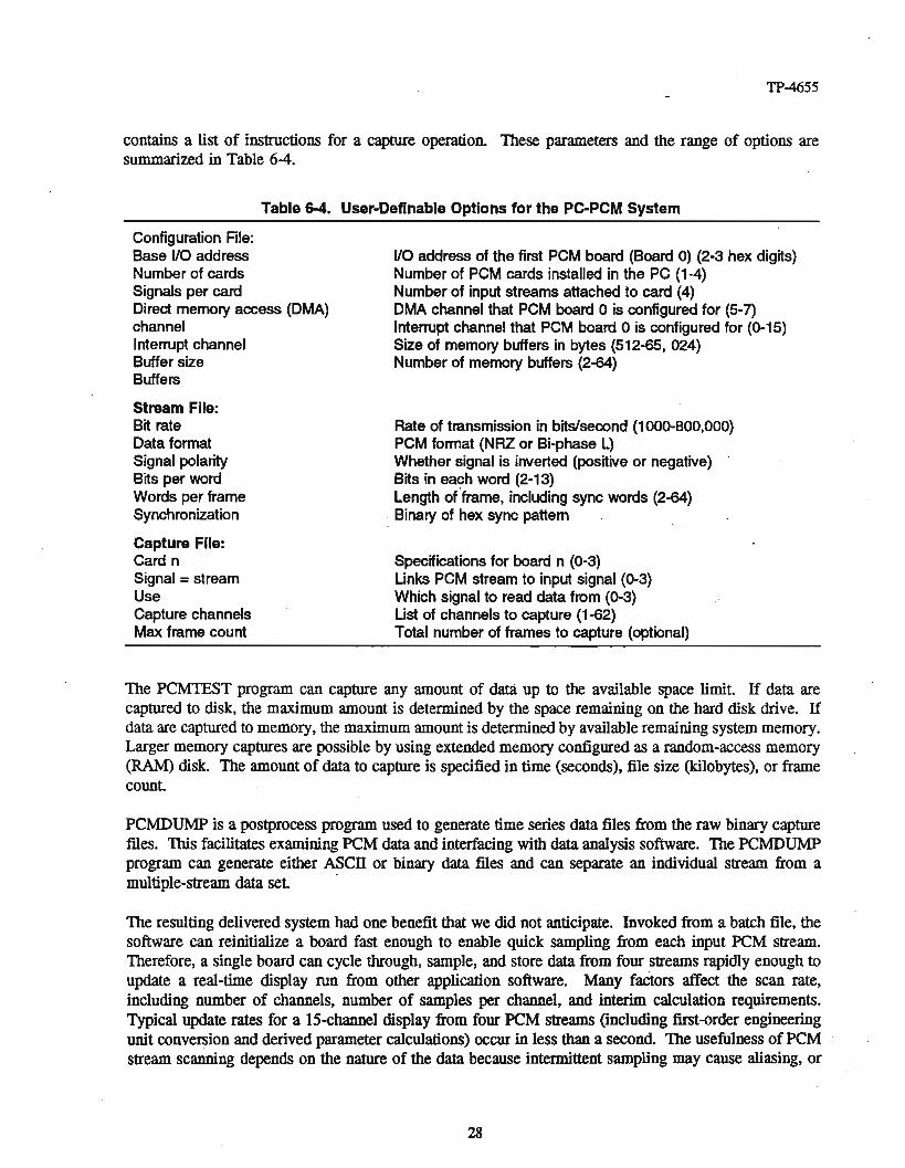
contains a list of instructions for a capture operation. These parameters and the range of options aresummarized in Table 6-4.
Table 6-4. User-Definable Options for the PC-PCM System
Configuration File:Base I/O addressNumber of cardsSignals per cardDirect memory access (DMA)channelInterrupt channelBuffer sizeBuffers
Stream File:Bit rateData formatSignal polarityBits per wordWords per frameSynchronization
Capture Rle:Card nSignal =streamUseCapture channelsMax frame count
I/O address of the first PCM board (Board 0) (2-3 hex digits)Number of PCM cards installed in the PC (1-4)Number of input streams attached to card (4)DMA channel that PCM board 0 is configured for (5-7)Interrupt channel that PCM board 0 is configured for (0-15)Size of memory buffers in bytes (512-65, 024)Number of memory buffers (2-64)
Rate of transmission in bits/second (1000-800,000)PCM format (NRZ or Bi-phase L)Whether signal is inverted (positive or negative)Bits in each word (2-13)Length ctframe, including sync words (2-64)
. Binary of hex sync pattem
Specifications for board n (0-3)Links PCM stream to input signal (0-3)Which signal to read data from (0-3)List of channels to capture (1-62)Total number of frames to capture (optional)
The PCMTEST program can capture any amount of data up to the available space limit. If data arecaptured to disk, the maximum amount is determined by the space remaining on the hard disk drive. Ifdataarecaptured to memory, the maximum amount is determined by available remaining system memory.Larger memory captures are possible by usingextended memory configured as a random-access memory(RAM) disk. The amount of datato capture is specified in time (seconds), file size (kilobytes), or framecount
PCMDUMP is a postprocess program used to generate time series data files fromthe raw binarycapturefiles. This facilitates examining PCM data and interfacing withdataanalysis software. ThePCMDUMPprogram can generate either ASCn or binary data files and can separate an individual stream from amultiple-stream dataset .
The resulting delivered system had one benefitthat we did not anticipate. Invoked from a batchfile, thesoftware can reinitialize a board fast enough to enable quick sampling from each input PCM stream.Therefore, a singleboard can cycle through, sample, and store data from four streams rapidly enough toupdate a real-time display run from other application software. Many factors affect the scan rate,including number of channels, number of samples per channel, and interim calculation requirements.Typical update rates for a 15-channel display from four PCM streams (including first-order engineeringunit conversion and derived parameter calculations) occurin less than a second The usefulness ofPCMstream scanning depends on the nature of the data because intermittent sampling may cause aliasing, or
28

TP-4655
transients may be missed. However, for many of our averageddataapplications, the monitoring of many.channels by scanning across multiple streams is very useful.
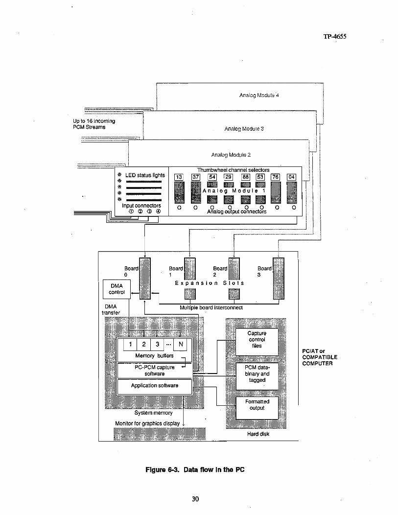
6.2.4 Data Flow in the Computer
A clear understanding of the data- flow inside the computeris helpful in understanding the capabilities andlimitations of the PCM decoder board. Figure 6-3 shows the dataflow inside the PC, described below.PCM data streams can be input directly to the PC-PCM decoder board or interfaced through an analogmodule. The analogmodule allows the user to selectup to eight desiredchannels (via thumb-wheel dials)for analog output The analog voltage output can be selected in the 10- or 20-V span range, bipolar orunipolar. The analogmodule also interfacesthe PC-PCMboards to panel-mounted liquid-emitting diodes(LEDs) to inform the user of system status. (TIle status LED panel could also be built independently ofthe D/A system.) Status lights indicate captureactivity, PLL status, frame sync status, PC memorystatus,and error state.
The PCM decoder boards are under the control of the capture software running in PC system memory.This program can be ron on its own or via user application software. The capture program writesbinary-format tagged PCM data. Each dataword is tagged with its correspondingPCM board number.Captured data can be accessed by the applicationprogram through memory or disk files.
The capture softwarereads user-definedparameters from the capture control disk files, then initiates andterminates the capture operation. Before initiating capture, the direct memory access (DMA) controlleris initialized to define the starting address and size of the first memory buffer. The DMA controllerhasa special address generator that allows it to move data from the PCM decoder card to the addresses -inmemory. When capture is initiated, the DMA controller moves data from the PCM board to the rustmemory buffer in 16-bit words. When the buffer is full, the DMA controller informs the PCM decodercard, which in turn generates an interrupt to the capture software.
Upon receiving the interrupt, the capture softwarereinitializes the DMA controller to transfer datato thenext availablebuffer. This process is repeateduntil the capture is complete. While the buffers are beingfilled, application software could simultaneously access the data in the full buffers. Flags are providedfor each buffer to define when they are full, empty, or in use.
This structurehas many advantages. First, the DMA controllermoves datafrom the PCM decoderboardto memory more quickly than a software transfer does, and it is an independent process. The DMAcontroller actually takes over the PC!AT bus when data are transferred and does not burden themicroprocessor, This makesthe application softwaresimplerand moreefficient Memorybuffersprovideanotheradvantage. When dataare beingtransferredto the hard disk, these buffers store datauntil the harddisk can rotate to the proper sector to write the data. Without these buffers, data would be lost
6.2.5 Data Capture Performance Estimates
In single-stream mode, a typical PC/AT can capture PCM data to disk at rates up to 800 Kbitslsec. Formultiple-stream disk capture, quantifying performance is difficult due to many possible combinations ofPCM stream rates and PC capabilities. An algorithm for estimating disk data capture rate is
nCR = 16 III (BR / BPW) * (CWPFIWPF)
29
(6-1)
TP-4655
where:
DCR = PC data disk capture rate in bits/secondBR = Incoming PCM bit rate in bits/second
BPW = Data bits per PCM wordCWPF = Words captured per PCM frame
WPF = Total words Per PCM frame, including sync.
The data capture rate (DCR) for multiple cards is the sum of the DCRs for each individual card.
To provide some rough performance estimates, a test was run using four PC-PCM boards installed in a25-MHz 80386-based PC. A PCM simulator was used to generate 62 channels of 12-bit words inBi-Phase L format with2 syncwords per frame. Datawere captured to contiguous blocksof disk storagespace. The PC system could continuously capture to disk all channels of data from two 800-Kbitlsecstreams. It could alsocapture all channels from four400-Kbitlsec streams. The maximum occurred withthree 800-Kbitlsec streams, each capturing 45 channels. At rates abovethis, the hard disk couldnot keepup with incoming data, and capture was terminated by a buffer overflow error condition.
Based on Eq. 6-1, the corresponding upper limit of disk data capture for this configuration isapproximately 2.25 Mbitslsec. The PC's hard disk was rated at 10 Molts/sec, indicating that the requiredPC disk speed should be 4 to 5 times the maximum data capture rate in order to ensure adequateperformance. Manyfactors are likely to affect these values, including disk fragmentation, disk interfacetype, disk interleave, buffer size, CPU speed, and other installed PC options.
With the same system configuration, there were no performance limits when capturing datato memory.PCM data fromfour 64-channel, 800-Kbitlsec streams weresuccessfully captured to an extended memoryRAM disk. This is useful for providing higher-rate capture, but data quantities are limited because ofmemory restrictions. Large amounts of memory are less common and more expensive than comparabledisk space.
6.2.6 Architecture of PCM Decoder Board
The PCM decoder boardhas a programmable bit detector for extracting the ones and zeros fromthe PCMsignal. These are passedon to the frame and wordprocessing sectionwhere the words are extracted andthen interfaced to the PC. The following paragraphs discuss each of these in detail.
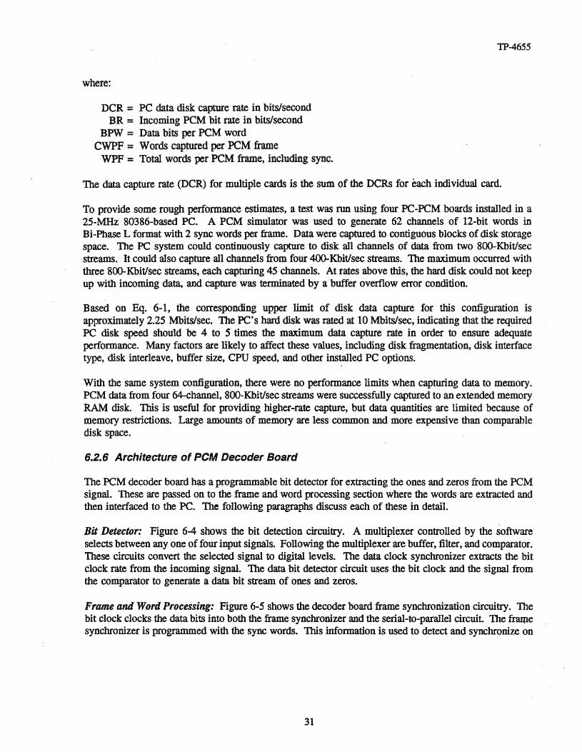
Bit Detector: Figure 6-4 shows the bit detection circuitry. A multiplexer controlled by the softwareselects betweenanyone of fourinput signals. Following the multiplexer arebuffer, :filter, andcomparator.These circuits convert the selected signal to digital levels. The data clock synchronizer extracts the bitclock rate from the incoming signal. The data bit detector circuituses the bit clock and the signal fromthe comparator to generate a data bit stream of ones and zeros.
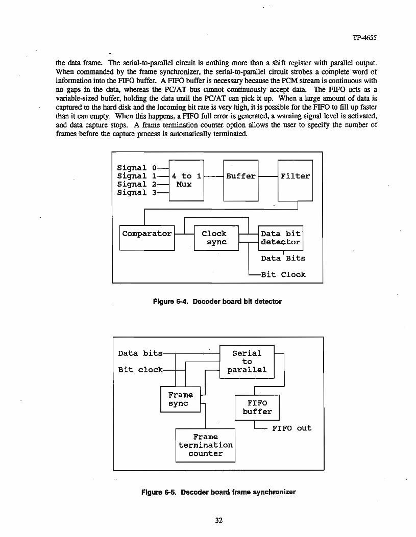
Frame andWord Processing: Figure6-5 shows the decoder boardframe synchronization circuitry. Thebit clockclocks the data bits into both the frame synchronizer andthe serial-to-parallel circuit. Theframesynchronizer is programmed with the sync words. This information is used to detectand synchronize on
31
TP-4655
the data frame. The serial-to-parallel circuit is nothing more than a shift register with parallel output.When commanded by the frame synchronizer. the serial-to-parallel circuit strobes a complete word ofinformation into the FIFO buffer. A FIFO buffer is necessary because the PCM stream is continuous withno gaps in the data, whereas the pC!AT bus cannot continuously accept data. The FIFO acts as avariable-sized buffer, holding the data until the PC/AT can pick it up. When a large amount of data iscaptured to the hard disk and the incoming bit rate is very high, it is possible for the FIFO to fill up fasterthan it can empty. When this happens. a FIFO full error is generated, a warning signal level is activated.and data capture stops. A frame termination counter option allows the user to specify the number offrames before the capture process is automatically terminated.
B~t Clock
Signal 0-Signal 1- 4 to 1 Buffer Filtersignal 2- Muxsignal 3-
0 - I
I IComparator Clock Data bitsync detector
Datal Bits
-I.
Figure 6-4. Decoder board bit detector
o out
s Serial -to
- parallel
Frame I
sync FIFObuffer
L FIFFrame
terminationcounter
Data bit
Bit clock
Figure 6-5. Decoder board frame synchronizer
32
TP-4655
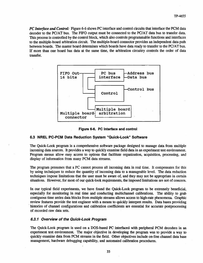
PCInterface andControl: Figure 6-6 shows PC interface and control circuits that interface the PCM datadecoder to the PCIAT bus. The FIFO output must be connected to the PCIAT data bus to transfer data.This process is controlled by the control block, which also controls programmable functions and interfacesto the multiple-board arbitration circuit The multiple-board connector provides an independent data pathbetween boards. The master board determines which boards have dataready to transfer to the PCIAT bus.If more than one board has data at the same timet the arbitration circuitry controls the order of datatransfer.
FIFO Out.---.----I16 bits
PC businterface
Control
Address busData bus
ontrol bus
MUltiple boardconnector
MUltiple boardarbitration
Figure 6-6. PC interface and control
6.3 NREL PC-PCM Data Reduction System IIQuick-Look" Software
The Quick-Look program is a comprehensive software package designed to manage data from multipleincoming data sources. It provides a way to quickly examine field data in an experiment test environment.Program menus allow easy access to options that facilitate organization, acquisition, processing, anddisplay of information from many PCM data streams.
The program presumes that a PC cannot process all incoming data in real time. It compensates for thisby using techniques to reduce the quantity of incoming data to a manageable level. The data reductiontechniques impose limitations that the user must be aware oft and they may not be appropriate in certainsituations. However, for most of our quick-look requirements, the imposed limitations are not of concern.
In our typical field experiments, we have found the Quick-Look program to be extremely beneficial,especially for monitoring in real time and conducting multichannel calibrations. The ability to grabcontiguous time series data blocks from multiple streams allows access to high-rate phenomena Graphicreview features provide the test engineer with a means to quickly interpret results. Data bases providinghistories of channel configurations and calibration coefficients are essential for accurate postprocessingof recorded raw data sets.
6.3.1 Overview of the Quick-Look Program
The Quick-Look program is used on a DOS-based PC interfaced with peripheral PCM decoders in anexperiment test environment. The major objective in developing the program was to provide a way toquickly examine data from PCM streams in the field. Other objectives include on-line channel data basemanagement, hardware debugging capability, and automated calibration procedures.
33
TP-4655 '
Menus are presented to the user enabling quick selectionof desired options. Each menu containsa title,followed by lines listing current availableoptions. The user uses the arrow keys to move a highlightedbar up and down to select the desired operation. From there, anotherlevel of menu options may appear,or option execution may begin.
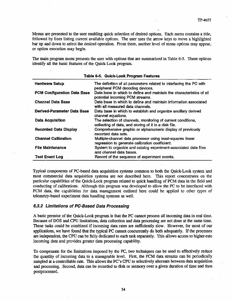
The main programmenu presents the user with options that are summarized in Table 6-5. These optionsidentify all the basic features of the Quick-Look program.
Table 6-5. Quick-Look Program Features
Hardware Setup The definitionof all parameters related to interfacing the PC withperipheral PCM decodingdevices.
PCM Configuration Data Base Data base in which to define and maintainthe characteristics of allpotential incoming PCM streams.
Channel Data Base Data base in which to define and maintain information associatedwith'all measured data channels.
Derived-Parameter Data Base Data base in which to establish and organize ancillary derivedchannel equations.
Data Acquisition The selectionof.channels, monitoring of current conditions,collecting of data, and storing of it in a disk file.
Recorded Data Display Comprehensive graphic or alphanumeric display of previouslyrecorded data sets.
Channel Calibration Multiple-channel data processor using least-squares linearregression to generate calibration coefficient.
File Maintenance Systemto organizeand catalog experiment-associated data filesand channel data bases.
Test Event Log Record of the sequenceof experiment events.
Typical components of PC-based data acquisition systems commonto both the Quick-Look system andmost commercial data acquisition systems are not described here. This report concentrates on theparticularcapabilities of the Quick-Look program related to quick handlingof PCM data in the field andconducting of calibrations. Although this program was developed to allow the PC to be interfaced withPCM data, the capabilities for data management outlined here could be applied to other types oftelemetry-based experiment data handling systems as well.
6.3.2 Limitations of PC-Based Data Processing
A basic premise of the Quick-Look programis that the PC cannot process all incomingdata in real time.Becauseof DOS and CPU limitations, data collectionand data processing are not done at the same time.These tasks could be combined if incoming data rates are sufficiently slow. However, for most of ourapplications. we have found that the typical PC cannot concurrently do both adequately. If the processesare independent, the CPU can be fully dedicatedto each task separately. This allowsaccessto higher-rateincoming data and provides greater data processing capability.
To compensate for the limitations imposed by the pc. two techniques can be used to effectively reducethe quantity of incoming data to a manageable level. First, the PCM data streams can be periodicallysampledat a controllable rate. This allowsthe PC's CPU to selectively alternate betweendata acquisitionand processing. Second.data can be recordedto disk or memoryover a given durationof time 'andthenpostprocessed.
34

TP-4655
These data reduction techniques impose restrictions that the user must be aware of, and they may not beappropriate in certain situations. For example, transients may be missed,or aliasing could be introduced.To provide data values representative of existing conditions, the data segments should be stationary timehistory records (Bendat and Piersol, 1980). The Quick-Look program provides many features that allowevaluation of time series data. It is up to the user to ensure that the data segments are sufficiently longand statistically meaningful to produce adequate results.
For most of our quick-lookrequirements, the limits imposed by the PC-based system are not of concern.In our typical field experiments, we have found this system to be extremely useful, especially·formonitoring current conditions and conducting channel calibrations. We do not, however,use this systemas a substitutefor full data processing. Usually, all PCM datastreams are recorded independently of thissystem to provide complete data sets for comprehensive postprocessing, as shown in Figure 6-2.
6.3.3 Interfacing a PC to ·the PCM Data Streams
The main function of the Quick-Look program is to interface a PC with PCM data. This requires sometype of PCM decoding hardwarewith the ability to transfer data into a PC. The data transfer can be donein a variety of ways, such as through a simple but slow serial communication port or complex but fastDMA buffers. The PCM decoding hardware can be outside or inside the PC. This report assumes thatPCM dataare providedto the Quick-Look programthrough a PC-basedPCM-decoding hardware systemdevelopedby NREL (Simms and Butterfield, 1990). The Quick-Look program could support other PCMdecoders if appropriate interfacedrivers were provided;however, some of the softwarefeatures describedhere depend on unique capabilities provided by the NREL decoding system.
The NREL PC-PCM decoding system consists of printed circuit boards (APEX Systems, 1988) that fitdirectly inside the chassis of a PCIAT or compatible computer and basic control software. PCM dataaredecoded on the board and DMA transferred to PC memory or disk. One board can decode one PCMstream at a time. Up to four boards can tie installed into a PC, permitting data from four streams to besimultaneously combined. The Quick-Look programbuilds all data files necessary for settingup PC-PCMboards and overlays control software to accomplish data acquisition.
The full complementof four boards in a PC allows the Quick-Look program to manage data from up to16PCM streams. Each board has four inputs and can be quickly reconfigured to cycle through the inputto sampledatafrom differentPCM streams. Variouscombinations of cyclic or concurrentacquisitioncanbe used. Maximumdata collectionrates vary, depending on hardware limitationsand other variables thatare discussed below. The boards support standard-format IRIG-compatible PCM streams with bit ratesin the range of 1000 to 800,000 bits/sec and a maximum of 64 data words (including sync) per frame.Based on 12-bit data resolution, channel sample rates from 1.3 to 33,000 Hz are possible.
The Quick-Look program assumes that each channel of input data is a time history record and that eachrecord has a constant sample rate. However, because data can originate from multiple PCM streams ofvarying rates, channels may have different sample rates. Data are transmitted to the program througharrays either in memory or on disk files. H multiplePC-PCMboards are used, datafrom up to four PCMstreams can be collected simultaneously. All incoming dataare meshed into a single file. After they arecollected, they are decoded for display by the Quick-Look program. H a single PC-PCM board is used,it is still possible to cycle throughand monitorup to four PCM streams,but simultaneous acquisition frommultiple streams is not possible. Software decoding of subcommutated or super-multiplexed PCM datais not supported.
35
TP-4655
To keep track of up to 16 PCM input, the Quick-Look program provides a locationmatrixinto which theuser assigns incoming PCM streams to their respective input locations. When data are requested from aparticular PCM stream, the program uses the matrix to determine how to set up acquisition so that thecorrectpcM streams are accessed.
During acquisition of PCM data, all values are based on raw counts, which are derived.from binary datawords that have been decodedfrom the PCM datastreams. Data resolution is determined by the numberof bits used to represent each measured data value. We typically use 12-bit resolution, which is 1 partin 212, corresponding to count values ranging from 0 to 4,095.The Quick-Look program interprets the raw count values provided by the PCM decoding hardware andconverts them to engineering units. As described above, because of the potentially large amount ofincoming dataand the limitations of the PC, the Quick-Look program does not acquire and process thedata simultaneously. It uses techniques of contiguous or sampled acquisition to reduce the volume ofincoming data to a manageable level. These techniques are described below.
6.3.4 Contiguous Data Acquisition
In contiguous data acquisition, data streamsare recorded as time historyrecordblockswith no gaps. Datafrom up to four streams can be acquired simultaneously to a disk file up to the limit of available diskspace. The datablocks are then postprocessed using features of the Quick-Look program or other dataanalysis programs. .
While contiguous data collection is occurring, no other process can run. After the block of data isacquired, summary statistics are presented on the monitor display. From these, the user can decidewhetherthe data set meets the necessary criteria.
The required number of samples is specifiedby the user as a time duration. The total resulting numberof data points depends on bit rate, numberof streams, and channels per stream. Large quantities of dataare not practical in this mode. Upward from 50,000 individual datavalues start to become difficult fortwo reasons:
1. Disk storage resources are quickly exhausted. Raw data are input to the program in an efficientbinary integer format However, to produce practical data sets, they are converted to engineering unitsand copied to an ASCII file in 80-column E12.3 format with corresponding time. This is very readable(and printable) but not storage efficient
2. It takes a longtimetoprocess. It is CPUintensive to decode and sort the raw binarydata. especiallyfor multi-board acquisition. Data from the PCM streams are intermeshed in one binary file as they areacquired. Each data valueis encodedwith a tag that identifies the streamand channel it came from. Thetag has to be removed from the data and used for sorting. The raw data valuesusually requireconversionto engineering units. Slower-rate data are interpolated to the rate of the fastest stream. The final data fileis chronologically organized as a time series,witheachrecordconsisting of a time value followed by datavalues from each requested channel for that time.
6.3.5 Real·Time Data Monitoring
Sampleddata acquisition is used to provide a real-time data monitoring capability. The incoming PCMstreams are periodically sampled to acquiresmall segments of contiguous data The segments are quicklyprocessed and displayed to show current conditions. The process is continuously repeated. Up to 135channels from any combination of incoming PCM streams can be displayed. Each representative value
36

TP-4655
for each channel is determined by averaging 1 to 10,000 contiguous samples. The user selects channelsfor display and defines an appropriate averaging interval.
Data monitoring is a cyclic repetitive process that is controlled by the Quick-Look program. This isshown in Figure 6-7 and can be described in three basic steps:
1. PCM-stream data acquisition is initiated to obtain datasegments from each requested channel. The. Quick-Look program overlays an independent data capture program that initializes the PCM decoding
boards, locks onto the PCM streams, and initiates datacapture. All PCM streams containing requestedchannels are sampled to obtain enough contiguous data frames for the required averaging interval. Dataare written to RAM disk, and control is returned to the Quick-Look program.
2. The Quick-Look program reads data from RAM disk and sorts by requested channel. Mean andstandard deviations are calculated for each channel from the total number of samples in the sample period.PCM data in units of counts can be converted to engineering units using the slope and offset from thechannel data base. If derived channels are requested, calculations are performed using equations fromthe derived-channel data base. Any combination of derive channels and measured channels can bedisplayed.
3. Resulting values are displayed on the screen in either raw PCM counts or engineering units. The mainreason for displaying counts is to conduct calibrations. The screen display is an alphanumericrepresentation of the current conditions for the requested set of data channels. The program monitors inpages of 15 channels each. Only one page is displayed at a time. The user can easily select from amongseveral pages by keying the desired page number. All pages are updated simultaneously after each setof data is processed. Each channel is displayed beginning with channel number, name, and units fromthe channel data base, followed by the current mean and standard deviation.
For example, selected channels would be displayed on the monitor in the following format:
201:Anemometer #1 (mls) .........................••... 1.067E+Ol (2.502E-Ol)307:Power Supply (Volts) 2.502E+OO (6.745E-02)402:Bending Moment (N-m) . . . . . . . . . . . . . . . . . . . . . . . . . . . .. 5.678E+02 (3.456E+Ol)
The first digit of the channel number identifies the PCM stream, and the next two digits identify the dataword The mean and standard deviation values continuously change as data monitoring cycles. Themonitor display may lag behind real time by a few seconds, depending on calculation overhead. For theCombined Experiment datastreams of Table 6-1, practical data monitor update rates of 1 to 10 sec wereeasily achievable.
At any time during data monitoring, data collection can be initiated via a user-entered keystroke. Thiscauses monitor-displayed mean and standard deviation values to be permanently recorded in an ASCn diskfile, The data monitor will continue to update and will note that data collection is in progress. Thecollection can be suspended and restarted at any time. Upon termination of data monitoring, collectionis stopped, and mean values for the entire period are calculated. These are inserted at the beginning ofthe data file, and the file is closed and saved. The user is notified of the file name, is shown the file forbrowsing, and has the option of printing a copy.
37
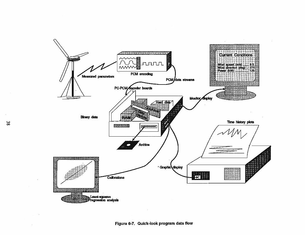

TP4655
6.3.6 Data Monitoring Features
Typically, the monitor displays current rapidly changing conditions. The current values are calculated byaveraging contiguous samples. Another level of averaging is also possible. A parallel monitor displayis available to show long-term averaged values that are determined from the current condition values.Keystrokes are used to toggle between the long- and short-term displays. For long-term averaging, currentdisplay values are summed for each channel (measured and derived) over the averaging period. At theend ofeachperiod the sums are divided bythe number ofscans, and the average display is updated. Theuser defines an appropriate long-term averaging period (typically in minutes).
Because up to 135 data channels can be monitored, it would be impractical to expect the user to re-enterthe list of desired channels each time he or she wants to monitor data. To overcome this, the programprovides a means of defining and saving collections of display channels. A user-defmed name isassociated with each collection. The user assembles a collection of channels, and the Quick-Look programadds it to a list of available selections. When data acquisition is initiated from the main menu, the useris presented with a menu containing the list of all available collections of channels and selects theappropriate one using the arrow keys. It is also possible to modify an existing collection, delete obsoleteones, and define new ones.
For real-time datamonitoring, a range-check feature exists that highlights the display when a value is outof range. The user enters the maximum and minimum allowable values for a particular channel in thechannel database. If a value is outside the range, it is displayed with a conspicuous red background.
Another type of real-time data monitor is provided in the form of a graphic bar chart display. This canbe invoked at any time during alphanumeric data monitoring via a user-entered keystroke. Up to 62measured channel values are graphically displayed.as bar graphs on the screen. The Quick-Look programsets up the bar chart display with the desired PCM stream configuration and channels. The bar chartmonitor shows data in units of counts and can be used on only one PCM stream at a time. Its displayupdate rate is very fast, typically many times per second. It is useful for quickly checking a large numberof channels at once because dead channels are readily detected and easily identified.
6.3.7 Factors Affecting Data Monitor Rates
The rate at which the data monitor display updates itself is affected by many factors. Some depend onwhich program options the user selects. Others are inherent in the hardware. Some of the factors are
1. CPU speed of the PC2. Number of channels to display3. Number of scans to average for each sample4. Whether engineering unit conversion is done5. Whether derived parameters are calculated6. Overhead of the PC-PCM board capture software7. Bit rate of the incoming PCM stream(s)8. PCM stream consistency and quality9. Whether data are captured to RAM or hard disk10. Whether simultaneous or cyclic acquisition is used11. Whether data collection is occurring.
39

TP-4655
6.3.8 Data Base of PCM Stream Configuration
TheQuick-Look program provides a form into which a setof configuration parameters defining eachPCMstream can be input The parameters are then usedto set up decoding hardware to access streams whosechannels are requested. The configuration parameters are
1. PCM stream title2. Number of data words per frame (data channels)3. Number of sync words per frame4. Binary sync bit pattern5. Bit rate in bits/second6. PCM data format (Bi-phase L or NRZ)7. Signal polarity8. Bits/word9. Samples to average.
6.3.9 Data Base of Channel Parameters
A data base is kept for each channel of each PCM stream. A maximum of 70 channels per stream isallowed. The data base consists of a set of user-definable parameters and corresponding data. For theCombined Experiment. the following parameters fields are used:
1. Channel description2. Sensor location3. Sensor type4. Sensor ID number5. Anti-alias filter setting6. Sample rate7. Engineering data units8. Slope (engineering units/count)9. Offset (engineering units)to. Range maximum11. Range minimum12. Reference channel for calibration13. Low, zero (mid), and high calibration values14. Flag to print mean values to a log file15. Date and time of latest revision.
Parameters 2 to 6 areavailable for bookkeeping purposes, andotherthanfor comprehensive printouts, theyare not used elsewhere in the program. Values do not have to be entered in these fields, Parameters 1and7 to 14areusedin various otherplaces in the software. Values mayneedto be entered in thesefieldsdepending on the program option selected.
The channel data base option of the Quick-Look program provides access to these parameters for anychannel on any PCM stream. The user is presented with a form on the screen that displays currentparameter values, which can easily be updated or modified. If any changes are made, a new version ofthe data base file is written and becomes the current version. Parameter 15 is updated automatically ifany changes are made in any field. •
40
TP-4655
Previous versions of the channel data base are retained so that a history of the channel, includingcalibration coefficients, is available. The program allows previous versions to easily be recovered. nusis especially useful for postprocessing raw PCM data recorded on tape, allowing ready access to datavalues in correct engineering units.
6.3.10 Derived Channel Data Base
A data·base of all derived channels is .maintained by the Quick-Look program. A derived channel canbe a function of many channels from multiple PCM streams. When the user selects the derived-channeldata base option, a simple form is presented in which the channel description and derived equation areentered. The equation may contain constants, functions, or measured channel numbers. Upon completion,the derived-channel information is saved and made available for use either in monitoring or generatingdata files.
6.3.11 Rapid Multi-Channel Calibration Capability
Only linear engineering unit conversions are provided, one slope and offset pair for each channel. Theslopes and offsets can be input manually into the channel data base, ifknown. They can also be generatedbased on measured data obtained during "calibration runs" and automatically inserted into the channel database. It is possible to quickly generate and update calibration coefficients for many channels from manyPCM streams simultaneously. There are four options for calibration runs:
1. 3-level highlmidllow calibration data2. 2-level highllow calibration data3. I-level zero calibrations (determines offset only)4. A function of another "reference" data channel.
For the first two options, PCM count data are collected at the constant calibration levels for a shortduration of time and stored in a file. The channel data base contains a value in engineering units thatshould coincide with the measured count value at each level. The count data are read from a file andcompared to the reference values. A least-squares regression line is generated from which a slope andoffset are found, and correlation statistics are calculated.
For the third option, count values corresponding to the channel zero (or any known level) are stored toa file. The data base zero value is used as a reference, and a new offset is calculated.
. For the fourth option, engineering unit data are concurrently measured from a reference channel used togenerate coefficients for the channels to be calibrated. The relation between the reference channel andthe channel to be calibrated is limited to a simple user-defined mathematical function entered in thechannel data base. A least-squares regression line is generated to obtain the relation between the twovariables. This allows a ramp calibration to be done, in which the data values are distributed over a widerange as opposed to discrete known levels.
Upon completion of a calibration run, the user is presented with a page of summary regression statistics,other information pertinent to the least-squares fit, and new calibration values. The user can opt to acceptor decline the cal coefficients based on these statistics. He or she can also set up criteria that automatethe acceptance process using defined tolerances. For example, the user can identify acceptable ranges ofstandard error and correlation coefficients. If the regression statistics are within the ranges, :calcoefficients are automatically accepted and inserted in the data base. This Provides a means of quickly
41

TP4655
calibrating many channels. It has proven very useful in the Combined Experiment, in which calibrationsof 128 pressure channels are required every 5 min of testing.
6.3.12 Event Log File
The Quick-Look program provides a means for maintaining a log of events that occur during anexperiment The user can set up a log file at any time. The log feature automatically notes when dataacquisition occurred and summarizes channels used and mean data values during the interval. If anychanges are made in the channel database, it is noted in the log that a new version was generated. If anychannels are recalibrated, their new calibration coefficients and regression statistics are included in the log.The user can easily enter comments, which will be time stamped.
6.3.13 Quick Review of Recorded Data
Upon completion of data collection to a file, the file is immediately available for review. It is presentedto the user and can be scanned and printed. Channel values can also be displayed easily using includedgraphics programs. Two- (2D) or three-dimensional (3D) plot capability is available. Basically, all theuser has to do is select a datafile, plot type, and desired channels. Available plot types are as follows:
• 2D time series plots: Channel data are plotted on the ordinate axis with time on the abscissa. Axes'maximum and minimum are automatically chosen based on datarange. Channel dataare plotted inappropriate units. A legend that uses the channel name to identify each curve is automaticallyincluded. Up to 10 channels of data can be displayed on one graph.
• 2D X-vs.-Yplots: Channel dataare plotted on both axes for comparison. A legend is generated fromthe name of each Y-axis channel to distinguish among multiple comparisons. Up to 10 comparisonscan be displayed on one graph.
• Custom 2D plots: This option provides the user with some flexibility to generate custom-format plots.
• 3D plotsoftime-vs.-channel-vs.-tJata value: This option provides a quick way to look at time seriesfrom many similar channels simultaneously. Time is plotted incrementally on the X axis. (It isassumed that the scans occur at even intervals of time.) Selected channels are plotted on the Y axisincrementally in the order in which they were selected. The datavalue magnitudes are plotted on theZ axis. The XYZ values are shown as a surface in three dimensions. Any deviation among channelsis readily noticeable on the plot surface. Appropriate surface display depends on the particular dataset, and display options are available to improve the view.
6.4 Combined Experiment Data Processing
Data processing requirements depend on what the dataare to be used for. Data from the Combined andUnsteady Aero Experiments are destined for a wide variety of different potential uses, and it is difficultto specify generic requirements. There are certain in-house projects and applications that dictate initialnecessities. Some of the subcontractors have also specified their needs. A channel measurement mayrequire greater accuracy for some applications than for others. We have attempted to incorporate themeasurement needs from all potential sources and, in addition, anticipate what future dataanalyses mightrequire. These measurement requirements are summarized in Appendix B.
The main objective is to provide channel data measurements within the defmed tolerance ranges to thespecified levels of confidence. It would be impossible, however, to make all measurements to these levels.
42
TP-4655
With 239 total channels, there is always the potential for some to be out of commission, not workingproperly, or not in calibration. It is therefore the test engineer's job to determine the severity of out-oftolerance data channels. This depends entirely on the objectives of the particular test It is the duty ofthe test engineer to ascertain what channel measurements are critical for that test. Ifcritical measurementsare within required tolerances, the dataset is considered valid, and those channels that are out of toleranceare listed and noted so that subsequent data users are aware of their status. For example, if a blade
.azimuth signal is out of tolerance, but the test requires non-rotating data, the azimuth signal accuracy isnot critical to the validity of the dataset If, however, critical channel measurements are out of tolerance,the data set is considered invalid and is not used. It is important for the test engineer to be able to assessthis in the field so that he knows that it is necessary to re-acquire the data set
Most of the tests conducted under the Combined Experiment require that pressure channels be withinspecified tolerances to a confidence level of one standard deviation. This pressure measurement accuracycriteria is typically the determining factor for accepting or declining a data set because these measurementsdemand the least allowable error. There are also varying requirements that certain other important datachannels be functioning properly. The test engineer weighs the results of the calibrations of the criticalchannels while considering the objectives of the particular test to determine if the data set is worth furtherpostprocessing. The test engineer has many tools at his disposal in the field for assessing data quality andcan usually successfully identify valid data sets. Not only can he perform calibrations, but he can alsomonitor conditions in real time, cross-check redundant measurements, check acceptability of derivedparameters, and scan channels for out-of-range data. This greatly reduces the amount of invalid datasubmitted for subsequent time-consuming postprocessing.
6.4.1 Measurement Accuracy
Under no circumstances do we use the manufacturer-specified accuracy of any transducer, signalconditioner, or PCM encoder. We also do not rely on manufacturer calibrations or manufacturerrecommended calibration intervals; Le., that transducers or equipment calibrated at recommended intervalswill unconditionally provide accurate results. Rather, accuracy is determined by conducting regularperiodic pre- and post-calibrations on the full data path of all measured channels. The results of thecalibrations are then used to specify measurement accuracy.
Pre- and post-calibration sequences were designedandare utilized to provide a direct measurement of dataaccuracy. Pre- and post-calibrations are performed on the complete data path of each channel for eachdata set Two criteria have to be met to ensure adequate calibrations. FIrSt, regression statistics resultingfrom calculated coefficients of each calibration are required to lie within specified error limits. Second,if the difference between the pre- and post-calibration coefficients exceeds the specified tolerance, datacollected during the interval between calibrations are considered out of tolerance for that channel.Measurement tolerances and calibration procedures for all channels are shown in Appendix B.
. Calibrations for all channels are conducted at time intervals sufficient to ensure the accuracy ofintermediate data and were determined from test experience. These time intervals vary from minutes tomonths, depending on the transducer or system component being calibrated and the required channelaccuracy. They are categorized according to calibration procedure and are listed in Section 6.4.3.
The objective in calibrating the full datapath is to measure the accuracy of all components of the dataacquisition system that affect data measurement This includes the transducer itself, connecting cables,signal conditioner, and AID converter. Full data path calibrations are conducted on all channels. For theCombined Experiment, they are performed in two basic ways:
43

TP-4655
1. Single-part or "end-to-end" calibriltWns: The most preferable way to calibrate a channel is todirectly measure the full-channel response using an external reference that produces a known result Thatway, all the components along the data path are calibrated together, and the accuracy of the full systemcan be calculated (i.e., blade pulls or reference pressure transducer).
Z. Two-part calibriltWns: For some channels, it is not possible -to calibrate the transducer in situ. Forthese, full-channel accuracy is determined from two calibrations, an electronics calibration and a transducercalibration. The electronics calibration is performed by replacing the transducer input signal with a known
- precision reference voltage. This measures the response of the electronic portion of the signal path(mainly the signal conditioning and AID conversion systems), which is usually most prone to drift. Theaccuracy of the transducer is determined by external pre- and post-calibration to ensure that it remainedwithin tolerance during use. A good example of this is the wind speed channels, where the electronicsare drift calibrated with each data set, but the anemometers themselves are calibrated seasonally in thewind tunnel. In these cases, the root-mean-square (RMS) sum of the accuracy values from variouscomponent calibrations determined the overall channel accuracy.
Procedures for performing calibrations to produce measurement accuracy within required statisticalsignificance levels are detailed in the calibration procedure column of Appendix B. Those channels inwhich the transducer requires an external calibration (calibration procedure prefixed by an E) are two-partcalibrations. All other channels are calibrated with an end-to-end calibration. Some channels (such aspressures and strain gages) require two end-to-end calibrations, one to calculate slope and another tocalculate offset
The pre- and post-calibration strategy assumes that the channel measurement stayed within calibrationduring the intervening period. Obviously, this may not be the case, but because it is impossible tocontinuously calibrate channels, some assumptions have to be made. We have conducted many calibrationstudies to define appropriate calibration intervals necessary to ensure data accuracy. We have also devisedmany built-in "sanity checks," which are used to periodically check the data validity of important channels.
6.4.2 Features of the Custom Data Calibration System
It is the objective of the test engineer in the field to produce measurements that are within the tolerancelimits specified in Appendix B. It is very difficult, however, to completely ensure the accuracy of allchannels, considering the limited facilities and time available in the field. To guarantee that all channelmeasurements are within the required error tolerance limits is no small task, especially when each 10 minof operation requires re-calibration of at least 200 channels, some of them to extremely tight tolerancelimits (to calibrate pressure channels to .2% full-scale allowable error requires least-squares linearregression calculations on hundreds of data points for each channel). For that reason, a custom datacalibration system was developed with the specific objective of assisting the test engineer in the field.It provides a variety of tools to initially assess the accuracy of the data by performing calibrations andexamining important or critical channel measurements. This strategy has proven to bevery useful becausethe test engineer can quickly identify and eliminate out-of-tolerance data. It saves having to spend a lotof time and effort postprocessing data sets only to find that they contain worthless information. It alsolets the test engineer immediately know the status of the test matrix. Subsequent rigorous postprocessinganalyses are performed to provide final data accuracy values.
The custom data calibration system consists of 3 COmponents:
1. Microprocessor-controlled, rotor-mounted PSC: As seen in Appendix B, pressure measurements arethose that require the most stringent calibration tolerances. The PSC was designed and built to provide
44
TP-4655
in-flight National Institute of Science and Technology-traceable reference calibration pressures to allpressure ports. While the machine is operating, the test engineer can initiate a command from the groundthat causes the pressure transducers to replace the measured tap pressures with reference calibrationpressure on all 128 ports simultaneously. The reference pressure ramps up and down across themeasurement range to allow acquisition and calibration of each channel to the required level of statisticalsignificance. The PSC also provides necessary anti-alias filtering and high-quality signal conditioning onall incoming analog pressure measurements to minimize drift and ensure data accuracy.
2. High- and low-calibration shunt system: For some channels, it is impossible or unnecessary toperform a completeend-to-end calibration in the field. A good example is wind speed. The anemometersonly require annual calibration in the wind tunnel. The electronics, however, from the output of thetransducers through the signal conditioning and data acquisition system, require more frequent calibrationto compensate for drift. This is done by periodically replacing incoming transducer voltages with a knownprecision reference voltage. A single-point calibration is used to compensate for electronics drift byproviding a reference for re-calculating the channel offset in engineering units. A two-point calibrationcan be used to provide a slope check.
3. PC-based Quick-Look automated calibration system: The experiment test environment rules out theuse of significant resources in the field to verify calibration results. We therefore developed the QuickLook system, which is a PC-based PCM data processing package. It simplifies the process of acquiringselected sets of channel data during calibration intervals and then automates generating engineering unitcalibration coefficients and maintaining data bases of calibration histories. It also allows easy examinationand channel cross-checking in real time. The Quick-Look system combines custom-developed PCMdecoding hardware boards with a custom-written software analysis package. The hardware boards areinserted into a PC to convert incoming PCM stream data to disk files. This capability is described indetail in Simms (1990). The software was developed to provide the test engineer with a quick way toconduct multi-channel calibrations in the field. It is described in Simms and Butterfield (1990).
It would have been impossible to conduct the frequent calibrations required by the Combined Experimentand manage all the resulting information without custom data calibration system capabilities. In previousexperiments, we had to rely on laboratory-based postprocessing analyses to provide calibration results.Often, by that time, it was too late to go back into the field if subtle or overlooked problems surfacedwhen analyzing data. At the time of planning for the Combined Experiment, we only had a basic fieldsystem that could display a limited number of channel data values. Cost-effective commercial systemsthat could provide more comprehensive field analysis were not available. We therefore had no choice butto develop our own system to satisfy specific field data verification requirements For that reason, theQuick-Look system, in conjunction with PC-PCM decoding boards, was developed. Recently, low-costcommercial PC-based systems have become available that provide expanded field display capability; thesemight be useful in future tests.
6.4.3 Combined Experiment Calibration Sequences
The calibration sequences can be classified into three categories: automatic, manual, and external. Thesequences are performed at various time intervals to provide information necessary to computemeasurement accuracy. Specific procedures are defined that the test engineer must undertake in order toperform the calibration sequences.
1. Automatic calibrations are those initiated by the test engineer in the test shed to automaticallyinvokethe calibration sequence and cause data channels to measure calibration data Automatic calibrations areused to calibrate the most sensitive channels (those that require the highest measurement tolerances). They
45

TP-4655
are usually conducted immediately before and after a dataevent and are directly recorded to the 14-trackdata tape. There is not enough time to process the results of these calibrations during data acquisitionbecause the objective is to get the calibration sequences as close as possible in time to the actual dataevent. The four types of automatic calibrations performed in the Combined/Unsteady Aero Experimentsare shown in Table 6-6.
Table 6-6. Automatic Calibration Procedures
procedure Description
A1 PCM 2&3 high and low shunt calibrationA2 Strain gage slow rotationsA3 Pressure system ramp calibrationA4 Pressure system short-line zero
calibration
Calibrate
OffsetOffsetSlopeOffset
2. Manual calibration requires the test engineer to set up and conduct the calibration in the field on thetransducers in situ. These calibrations should be performed within the specified time intervals. These aredone using the Quick-Look system, and all data are saved as PC data sets in units of raw counts. Twosets, a pre- and a post-calibration, need to be done for each affected channel before fmal accuracy valuescan be specified. The manual calibration procedures and recommended time intervals are shown inTable 6-7.
3. Extemai calibration requires the transducer to be removed and calibrated in the calibration lab or inthe wind tunnel. These calibrations require more effort and are typically done on channels that are verystable or require less measurement tolerance and do not need frequent calibration. The calibration resultsare worked up to ensure that all measurements are within the required accuracy. Two sets, a pre- andpost-calibration, need to be done for each transducer before final accuracy values can be specified.External calibration procedures are shown in Table 6-8. .
Table 6-7. Manual Calibration Procedures
Procedure Description Frequency Calibrate
M1 PCM 1 north MET electronics < 1 week Offset, M2 AOA transducers < 1 week Slope & OffsetM3 Blade pitch angle < 1 week Slope & OffsetM4 Machine yaw angle potentiometer < 1 month Slope & OffsetM5 Blade azimuth angle potentiometer < 1 month Slope & OffsetM6 VPA wind directions < 1 month Slope & OffsetM7 VPA wind elevations < 1 month Slope & OffsetM8 Blade pulls for blade strain gages < 1 month SlopeM9 Tower pull for tower strain gates < 1 year Slope & OffsetM10 Yaw pull for yaw moment < 1 year Slope & Offset
46

TP-4655
Table 6-8. External Calibration Procedures
Procedure Description Frequency Calibrate
E1 Anemometer calibrations in wind tunnel < 1 year SlopeE2 Differential pressure sensor in calibration lab < 1 year SlopeE3 Absolute pressure sensor in calibration lab < 1 year SlopeE4 Differential temperature sensor in calibration lab < 1 year SlopeE5 Absolute temperature sensor in calibration lab < 1 year SlopeE6 Powertransducers in calibration lab < 1 year Slope
The recommended frequency of calibration intervals is to be used only as a guide. The stated intervalsare based on test experience to provide required accuracy values. Exact timing is not critical becausecalibrating at these intervals does not guarantee data accuracy. What is importantis to performpre- andpost-calibrations. It should be the objective of the test engineerto see that all channelsare pre- and postcalibrated at appropriate times as close as possible to when experiment data events are recorded.·
6.4.4 Field Data Recording and Processing Requirements
A data event consistsof 10 min of recorded data, during which all required parameters are measured. Itis boundedby calibration sequences designedto ensuredata validity. All information necessary to conductrequiredcalibrations is recordedso that calibration sequences can be reproduced. It is most preferable todirectly record raw PCM count data coming from channels during calibration sequences. From these,count to engineering unit conversions are derived. Each 14-track tape should contain two data events,preceded and followed by the appropriate automatic calibration sequences as defined in Table 6-9.
Calibrations 8 through 11 are optional if events 1 and 2 are done within an hour. The overall objectiveis for all channels of each data event to have a pre- and a post-calibration sequence recorded on tape.Over a longer term, manualand externalcalibrations shouldbe performed in a timely fashion to maintaindata base calibration coefficients up to date and to guarantee data accuracy. A hypothetical schedule isshown in Table 6-10 that assumes an experiment conducted over a 6-monthperiod in which various setsof data events are collected. The pre- and post-calibrations should be performed as close to the dataeventsas practical. All data are recordedon the Quick-Look systemand calibration coefficients generatedaccording to prescribedmethods. Some of the intermediate calibrations could be omitted if data sets arerecorded close enough together in time.
All information necessary to generate calibration coefficients for all measured channels is available to thetest engineerin the field. The calibration procedures are Performed by the test engineer at required timeintervalsto provide the information necessary to assessdata accuracy and to determine if the data sets arevalid or need to be re-acquired. The test engineer can work up the data at any convenienttime after adata event or tape has been collected.
In addition to conducting calibration, other methods have been devised to ensure that critical datameasurements are valid. These methods depend entirely on the channels being measured and the .availability of built-inredundancy or cross-checking measurements. For example, to ensure that the VPAanemometers are functioning correctly, we have found that long-term averages to check horizontal windstratification will readily pinpointout-of-calibration anemometers. For verifying pressure measurements,we have wind tunnel data from three independent sources in whichpressuredistributions as an AOA
47

TP-4655
Table 6-9. Event Acquisition Procedure
# Type
1. A12. A23. A34. A45.6. A47. A38. A29. A110. A111. A212. A313. A414.15. A416. A317. A218. A1
. Description
Pre-PCM 2&3 high and low calibrationsPre-slow rotationsPre-pressure systems ramp calibrationPre-pressure system zero calibration
Post-pressure system zero calibrationPost-pressure system ramp calibrationPost-slow rotationsPost-PCM 2&3 high and low calibrationsPre-PCM 2&3 high and low calibrationsPre-slow rotations
. Pre-pressure system ramp calibrationPre-pressure system zero calibration
Post-pressure system zero calibration.Post-pressure system ramp calibrationPost-slow rotationsPost-PCM 2&3 high and low calibrations
Time
< 1 hour prior to event 1< 1 hour prior to event 1Immediately prior to event 1Immediately prior to event 1Event 1:10 min of run dataImmediately following event 1Immediately following event 1< 1 hour after event 1 (can sub 10 or17)< 1 hour after event 1 (can sub 9 or18)< 1 hour prior to event 2 (can sub 1or 9)< 1 hour prior to event 2 (can sub 2or 8)Immediately prior to event 2Immediately prior to event 2Event 2:10 min of run dataImmediately following event 2Immediately following event 2< 1 hour after event 2< 1 hour after event 2
Table 6-10. Six-month Experiment Acquisition Procedure
# Type Description Time
1. E1 Pre-wind tunnel calibrations Up to 2 months before experiment2. E2-E6 Pre-calibration lab transducer calibrations Up to 2 months before experiment3. M9, M10 Pre-tower and yaw pull calibrations Up to 2 months before experiment4. M4-M8 Pre-event set #1 in situ transducer calibrations Up to 2 weeks before event set #15. M1-M3 Pre-event set #1 critical calibrations Up to 3 days before event set #16. 1 week of Data Events set #1 (See Table 6-9)7. M1-M3 Post-event set #1 critical calibrations Up to 3 days after event set #18. M4-M8 Post-event set #1 in situ transducer calibrations Up to 2 weeks after event set #19. M4-M8 Pre-event set #2 in situ transducer calibrations Up to 2 weeks before event set #210. M1-M3 Pre-event set #2 critical calibrations Up to 3 days before event set #211. 1 week of Data Events Set #2 (see Table 6-9)12. M1-M3 Post-event set #2 critical calibrations Up to 3 days after event set #213. M4-M8 Post-event set #2 in situ transducer calibrations Up to 2 weeks after event set #1
n-2n-1n
M9, M10E2-E6E1
Post-tower and yaw pull calibrationsPost-calibration lab transducer calibrationsPost-wind tunnel calibrations
48
Up to 2 months after experimentUp to 2 months after experimentUp to 2 months after equipment
TP-4655
function are documented We have found that pressure dismbutiondata binned according to the AOAis a good way to validate pressure measurements. These and other techniques are built into variousprocessing routines that are used to check and verify critical measurements.
6.4.5 Comprehensive Data Postprocessing
As stated above, final channel accuracy values cannot be calculated until all post-event calibrationprocedures have been performed and processed. All post-calibrations should be performed as soon aspossible afterthe experiment has been completed For that reason, it is especially important to removeanemometers or other transducers so that they are not damaged if they cannot immediately be postcalibrated. After post-calibrations, resultingmeasurement accuracies for all channelsshould be calculatedand incorporated'into thechannel data base for use in subsequentcomprehensive postprocessing analysis.
Many subsequentprocessesare applied to the data sets duringthepostprocessing phase. All channel dataare reduced to sample rates, shown in Appendix C, by decimation and filtering. This requires the use ofvariouscomputersystemsand softwarepackages,as shownin Figure 6-8. These proceduresare describedfurther in other reports and are summarized below:
1. Record PCM streams and time code to I4-track analog tape.
2. Perform Quick-Look display and analysis in the field
3. Generate calibration coefficients for all channels using Quick-Looksystem.
4. Associate and assemble appropriate calibrationcoefficientswith each channel for each Io-min dataset
5. Make two passes through the NREIlFairchild-Weston PCM Telemetry Data Reduction System toreduce and combine PCM streams into two groups of three streams each; output binary data sets todigital 9-track tape.
6. Load digital tape stream sets into UNIX system.
7. Use custom UNIXlCsoftware to combinetwo groupsof three streamseach into one continuoustimeseries that contains all six streams combinedto I-msec precision.
8. Use custom·UNIXlC software toa. Convert counts to engineering unitsb. Convert multi-rate data to common rate of 1.92 msec (520.83 Hz)c. Generate secondary derived parametersd Smooth azimuth angle signal for azimuth averaginge. Store data sets to optical media.
9. Use GENPRO'toa. Low-pass filter all channels to 4O-Hz bandwidthb. Low-pass filter all channels to Io-Hz bandwidthc. Low-pass filter all channels to I-Hz bandwidthd, Interpolate and smooth low-rate data to higher ratese. Generate power spectra for selected channelsf. Generate statistics for all data sets.
49
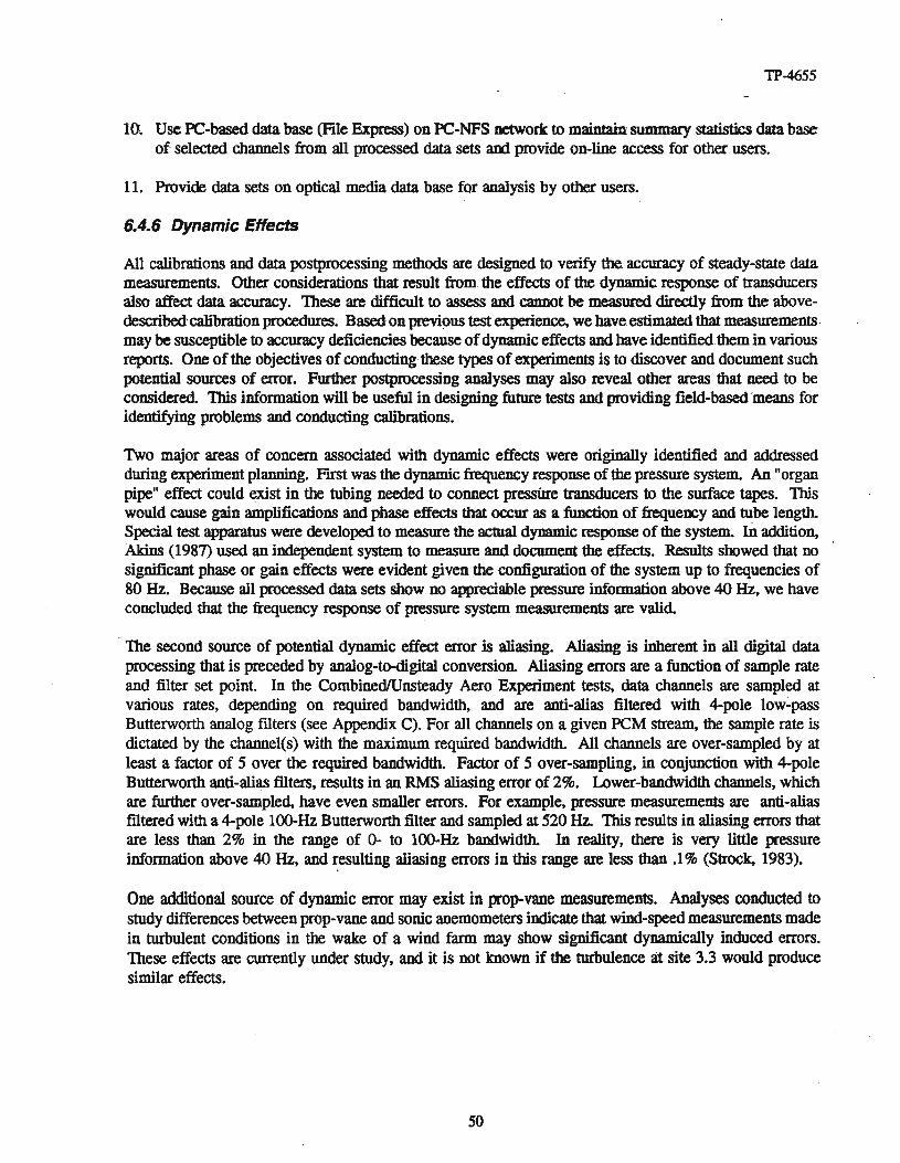
TP-4655
10. Use PC-based data base (File Express) on PC-NFS network to maintajn,summary statistics data baseof selected channels from all processed data sets and provide on-line access for other users.
11. Provide data sets on optical media data base for analysis by other users.
6.4.6 Dynamic Effects
All calibrations and datapostprocessing methods are designed to verify the accuracy of steady-state datameasurements. Other considerations that result from the effects of the dynamic response of transducersalso affect data accuracy. These are difficult to assess and cannot be measured directly from the abovedescribedcalibration procedures. Basedon previous test experience, we have estimated thatmeasurements,may be susceptible to accuracy deficiencies because ofdynamic effects and have identified them in variousreports. Oneof the objectives of conducting these types of experiments is to discover and document suchpotential sources of error. Further postprocessing analyses may also reveal other areas that need to beconsidered. This information will be useful in designing future tests and providing fleld-basedmeans foridentifying problems and conducting calibrations.
Two major areas of concern associated with dynamic effects were originally identified and addressedduring experiment planning. F.1!St was the dynamic frequency response of the pressure system. An "organpipe" effect could exist in the tubing needed to connect pressure transducers to the surface tapes. Thiswould cause gain amplifications and phase effects that occur as a function of frequency and tube length.Special test apparatus were developed to measure the actual dynamic response of the system. ID. addition,Akins (1987) used an independent system to measure and document the effects. Results showed that nosignificant phase or gain effects were evident given the configuration of the system up to frequencies of80 Hz. Because all processed data sets show no appreciable pressure information above 40 Hz, we haveconcluded that the frequency response of pressure system measurements are valid
The second source of potential dynamic effect error is aliasing. Aliasing is inherent in all digital dataprocessing that is preceded by analog-to-digital conversion. Aliasing errors are a function of sample rateand filter set point. In the CombinedlUnsteady Aero Experiment tests, data channels are sampled atvarious rates, depending on required bandwidth, and are anti-alias filtered with 4-pole low-passButterworth analog filters (see Appendix C). For all channels on a givenPCM stream, the sample rate isdictated by the channel(s) with the maximum required bandwidth. All channels are over-sampled by atleast a factor of 5 over the required bandwidth. Factor of 5 over-sampling, in conjunction with 4-poleButterworth anti-alias filters, results in an RMS aliasing error of 2%. Lower-bandwidth channels, whichare further over-sampled, have even smaller errors. For example, pressure measurements are anti-aliasfiltered with a 4-pole l00-Hz Butterworth filter and sampled at 520 Hz. This results in aliasing errors thatare less than 2% in the range of 0- to l00-Hz bandwidth. In reality, there is very little pressureinformation above 40 Hz, and resulting aliasing errors in this range are less than .1% (Strock, 1983).
One additional source of dynamic error may exist in prop-vane measurements. Analyses conducted tostudy differences between prop-vane and sonic anemometers indicate that wind-speed measurements madein turbulent conditions in the wake of a wind farm may show significant dynamically induced errors.These effects are currently under study, and it is not known if the turbulence at site 3.3 would producesimilar effects.
50

TP-4655
North Vertical Local Strain/ 30t & 63%&Met. Plane Metl SO% 47% Pressure
Tower Array Turbine Pressure Pressure & AOA's
11 213
14 Is 1
9
PCM Data streams
•14-TrackAnalog
Tape
Playback
PCM Data Streams
-PC
Quick-Look~--------~
System
SetupFiles(cals)
QuickLookData
Display
Dataverification
PCM Data Reduction:- 1/2 Tape speed (15 ips)- 5-minute record blocks- 2-pass process- output digital values
Fairchild/WestonPCM TelemetryEXPERT System
Data Archive:- Raw binary integers:- 234 Channels- 93,444 samples/sec- 11.2 Mbyte/min
Combine I------t Process i---tf------f opticalData Data Archive
Pass 1 passl2
PCM 4,8,1 PCM 9,2,39-track 9-tracktape tape
I
MASSCOMPUNIX
System
IntermediateData Storage/Transfer
I
Figure 6-8. Combined experiment phase II data processing plan
51

TP-4655
7.0 Wind Tunnel Testing
Wind tunnel data were used as reference data sets to compare with wind turbine data because this is thetype of datathat is used by designers as input to performance and structural design codes. For this reason,it was important to have an extensive data base for all operating conditions tested in the field. It was alsoimportant that this data base correspond to the exact airfoil under test. The wind tunnel data shouldrepresent the same chord, Reynolds number range, AOA range, pressure tap locations, and surfaceimperfections. Unfortunately, meeting all these criteria with one dataset measured from one wind tunnelwas not possible. For this reason, several wind tunnel tests were run; each one satisfied a different aspectof the required reference data set These different wind tunnel test programs are described in this section.
The airfoil chosen for the Combined Experiment was the S809, as mentioned earlier. This airfoil waschosen because;it was developed specifically for wind turbine applications, there was a wind tunnel database available from the Delft wind tunnel in The Netherlands, and NREL had extensive airfoil designanalysis results from the Eppler design code (Somers, 1989).
7.1 DELFT Tunnel Tests. .
The objectives of the Delft wind tunnel tests were to confirm the analytical design of the airfoil and tocalibrate the analysis code used to perform the design. To meet these Objectives, an extremely accurate600.Q-mm (23.6-in.) chord model was fabricated from aluminum and buffed to a surface finish that was .within 0.1 mm (0.004 in.) of the specified airfoil coordinates. Pressure taps were staggered on upper andlower surfaces at 108 locations. This level of model accuracy was necessary for model validation but wasnot practical for operating field tests on the Combined Experiment rotor. Butterfield (I989a) describesthe differences between the accurate Delft model and the model used in field tests and in Ohio StateUniversity wind tunnel tests.
Appendix D contains a summary of Somers (1989). This summary includes a brief description of the testsetup and a subset of the total results from these tests.
7.2 Ohio State University (OSU) Wind Tunnel Tests
Airfoil test data can be affected by surface irregularities, pressure tap locations, trailing edge accuracy, andmany other test setup details. It was important that the reference data set represent the exact airfoil andinstrumentation configuration, so that differences detected between the rotating blade data and the windtunnel data could be attributed ·to rotating blade effects. It was also important to establish an unsteady(dynamic stall) reference data set
For these reasons, a second series of wind tunnel tests was conducted. These tests used a 2D model thatwas fabricated using the same molds used to make the test blade. This assured that the same surfaceirregularities, trailing edge accuracy, chord length, and pressure tap locations would exist on the windtunnel test model. The same pressure measurement instrumentation was used in the wind tunnel as onthe test turbine. The same AOA probe was used during these tests to assure any effects of the probewould be included in the reference data sets.
The OSU wind tunnel was an open-eircuit type with a .92 m x 1.5 m (3 ft x 5 ft) test section. The modelhad a O.46-m (I8-in.) chord length and spanned the O.92-m dimension of the tunnel. The pressure taplocations and pressure measurement instrumentation used was the same as that used on the Combined
52
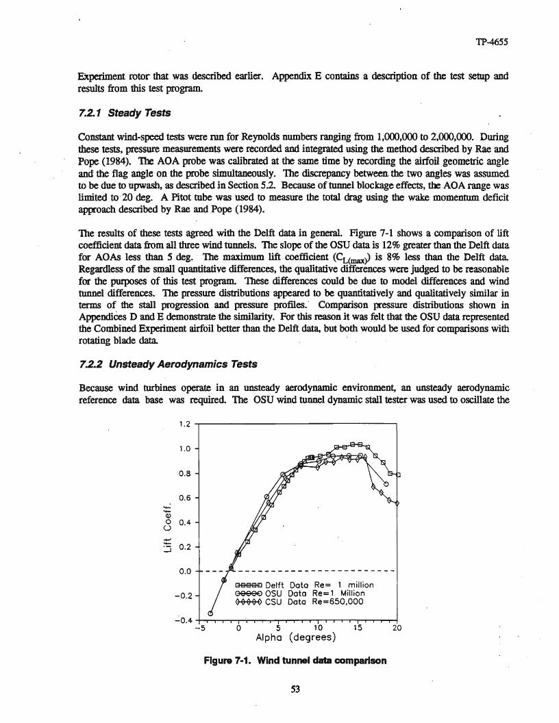
TP-4655
EXperiment rotor that was described earlier. Appendix E contains a description,of the test setup aridresults from this test program.
7.2.1 Steady Tests
Constant wind-speed tests were run for Reynolds numbers rangingfrom 1,000,000 to 2,000,000. Duringthese tests, pressure measurements were recorded.and integrated using the method described by Rae andPope (1984)~ The AOA probe was calibrated at the same time by recording the airfoil geometric angleand the flag angle'on the probe simultaneously. The discrepancy between thetwo angles was assumedto be due toupwash, as described in Section 5.2. Because of tunnel blockage effects, the AOA range waslimited to '20 deg. A Pitot tube was used to measure the total drag using the wake momentum deficitapproach described by Rae and Pope (1984).
The results of these tests agreed with the Delft data in general. Figure 7-1 shows a comparison of liftcoefficient data from all three wind tunnels. The slope of the OSU data is 12% greater than the Delft datafor AOAs less than 5 deg. ' The maximum lift coefficient (CL(max» is 8% less than the Delft data.Regardless of the small quantitative differences, the qualitative differences. were judged to be reasonablefor the purposes of this test program. These differences could be due to model differences and windtunnel differences. The pressure distributions appeared to be quantitatively and qualitatively similar interms of the stall progression and pressure profiles.' Comparison pressure distributions shown inAppendices D and E demonstrate the similarity. For this reason it was felt that the OSU data representedthe Combined Experiment airfoil better than the Delft data, but both would be used for comparisons withrotating blade data.
7.2.2 Unsteady Aerodynamics Tests
Because wind turbines operate in an unsteady aerodynamic environment, an unsteady aerodynamicreference data base was required. The OSU wind tunnel dynamic stall tester was used to oscillate the
1.2
1.0
0.8
0.6
----Q)
0 0.4U......-- 0.2:.:i
0.0
-0.2
-0.4-5
[3B8B€] Delft Data Re= 1 millionGeeeE) OSU Data Re= 1 Million~ CSU Data Re=650.000
o 5 10 15 20Alpha (degrees)
Figure 7-1. Wind tunnel data comparison
S3

TP-4655
model AOA in a sinusoidal manner. Various amplitudes and frequencies of oscillation were tested, andthe results are described in Appendix E.
7.2.3 Rough Airfoil Performance
Stall-controlledwind turbines suffer performance losses when the blade leading edges accumulatedebrisfrom insect impacts and airborne particulates. To document the sensitivity of the S809 to leading edgeroughness, buildup tests were conducted at OSU. Appendix E describes steady and unsteady airfoilperformance tests with roughness added to the leading edge of the model. The results of these testsprovided a reference data set for the rough blade tests conducted on the Combined Experiment turbine.The results of these tests are discussed in section 8.0.
7.3 Colorado State University Wind Tunnel
The Delft and OSU test data were limited to AOAs less than 22 deg and 20, respectively. Blockageeffects beyond these angles resulted in unacceptable errors. The Combined Experiment was focused onstall and deep stall airfoil performance that occurs at AOAs from IS to 30 deg. For this reason, anadditional wind tunnel test was conducted at the Colorado State University (CSU) Environmental WindTunnel. The large 3.66 m (12 ft) x 1 m (39 in.) test section available in this tunnel significantlyreducedthe blockage effects during high AOA testing.
7.3.1 Wind Tunnel Test Setup
The CSU Environmental Wind Tunnel was originally designed for studying flow over models of citiesand buildings. The test section was reduced to 3.66 m (12 ft.) x I m (39 in.), which allowed a I-m airfoiltest section to be inserted across the narrow dimension. This resulted in a wide test section that wouldminimize the blockage effects. The solid blockage was 0.28% using Thom's method (Rae and Pope,1984). Figure 7-2 shows the general layout of the tunnel and the modifications that were made for thistest. The modified,open-circuittunnel was capableof a maximumvelocityof 27 m/sec (a8 ftlsec), whichresulted in a Reynolds number, based on the 0.46-m (1.5-ft) chord, of 650,000. This Reynolds numbervalue is lower than the HAWT test conditions of 880,000 at the 80% blade span, but it was felt thatprevious wind tunnel data would accuratelydescribe the airfoil performancefor Reynolds number valuesfrom 750,000 to 3 million for AOA values less than 20 deg. Pressure distribution measurements weremade on the model along with pitot tube measurements 2 chord lengths displaced from each side of themodel and 1 chord length upwind of the model leading edge. Tunnel temperature, probe total pressure,local flow angle at 0.6 chord ahead of the leading edge, and model pitch angle relative to the tunnel axiswere also measured.
Normally, airfoil drag is measured by measuring the velocity profile in the wake of the airfoil and thenequating the momentum deficit in that wake to the total drag. This requires a movable Pitot tube or awake rake positioned downwind of the airfoil. These measurements were not possible to make on therotating wind turbine blade. There is also evidence that this technique is inaccurate when large-scaleseparationis present due to rotational flow in the wake. Because NREL's focus was stall behavior, wherelarge-scale separation is always present, it was decided that only pressure drag (CDn> would be measuredBecause CDp is determinedfrom pressure distributionintegrations(Rae and Pope, 1984),wind tunnel datacould be compared with HAWT data directly,
54
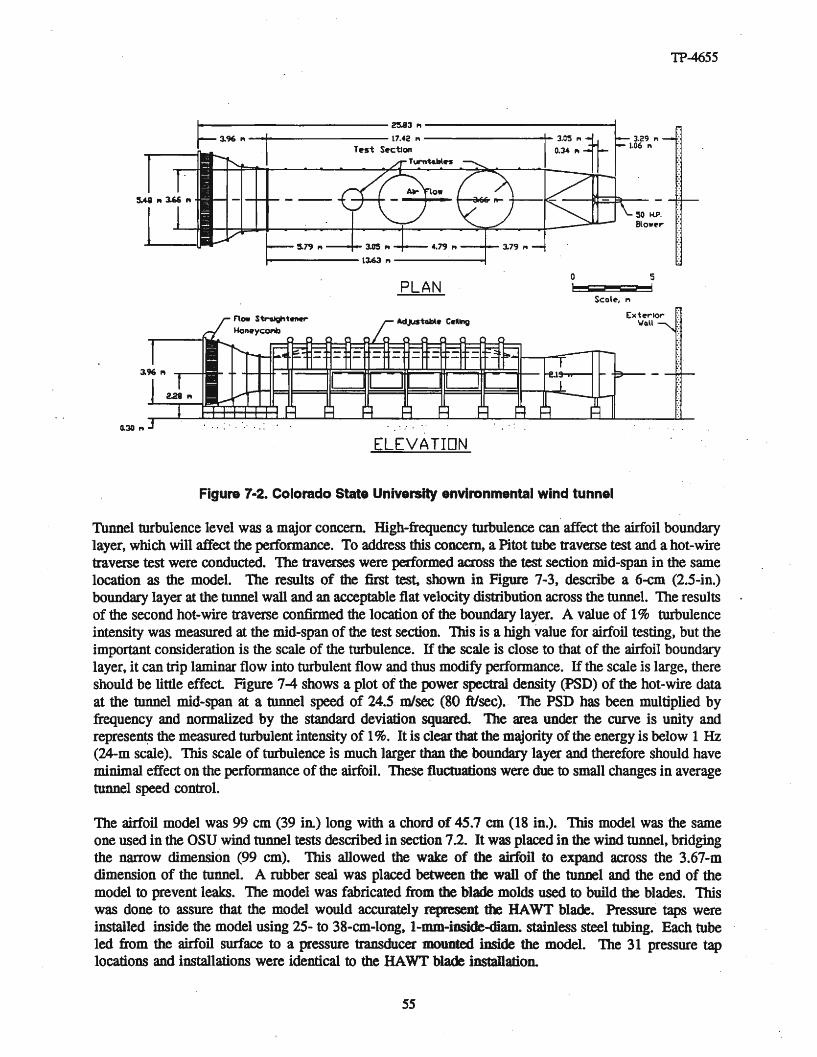
TP-4655
----------~3 .. -----------------17.42PI-------
T~st S~ctlon
T~"
0.30 PI ." .:"'."..:
PLAN
ELEVATION
a
---- Scale-, I"l
5
----'
Figure 7·2. Colorado State University environmental wind tunnel
Tunnel turbulence level was a major concern. High-frequency turbulence can affect the airfoil boundarylayer, which will affect the performance. To address this concern, a Pitot tube traverse test and a hot-wiretraverse test were conducted. The traverses were performed across the test section mid-span in the samelocation as the model. The results of the first test, shown in Figure 7-3, describe a 6-cm (2.S-in.)boundary layer at the tunnel wall and an acceptable flat velocity distribution across the tunnel. The resultsof the second hot-wire traverse confirmed the location of the boundary layer. A value of 1% turbulenceintensity was measured at the mid-span of the test section. This is a high value for airfoil testing, but theimportant consideration is the scale of the .turbulence. If the scale is close to that of the airfoil boundarylayer, it can trip laminar flow into turbulent flow and thus modify performance. If the scale is large, thereshould be little effect Figure 7-4 shows a plot of the power spectral density (PSD) of the hot-wire dataat the tunnel mid-span at a tunnel speed of 24.5 m1sec (80 ftIsec)e : The PSD has been multiplied byfrequency and normalized by the standard deviation squared. The area under the curve is unity andrepresents the measured turbulent intensity of 1%. It is clear that the majority of the energy is below 1 Hz(24-m scale). This scale of turbulence is much larger than the boundary layer and therefore should haveminimal effect on the performance of the airfoil. These fluctuations were due to small changes in averagetunnel .speed control. -
The airfoil model was 99 em (39 in.) long with a chord of 45.7 em (18 in.). This model was the sameone used in the OSU wind tunnel tests described in section 7.2. It was placed in the wind tunnel, bridgingthe narrow dimension (99 em). This allowed the wake of the airfoil to expand across the 3.67-mdimension of the tunnel. A rubber seal was placed between the wall of the tunnel and the end of themodel to prevent leaks. The model was fabricated from the blade molds used to build the blades. Thiswas done to assure that the model would accurately represent the HAWT blade. Pressure taps wereinstalled inside the model using 25- to 38-cm-Iong, I-mm-inside-diam. stainless steel tubing. Each tubeled from the airfoil surface to a pressure transducer mounted inside the model. The 31 pressure taplocations and installations were identical to the HAWT blade installation.
55
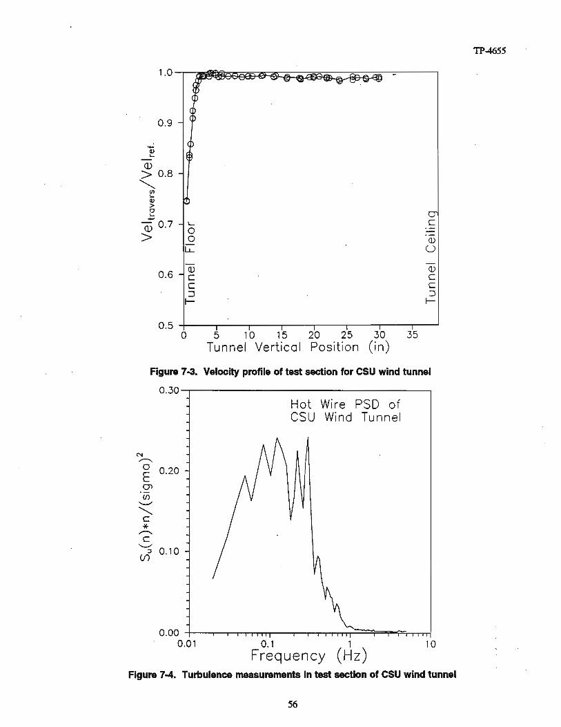
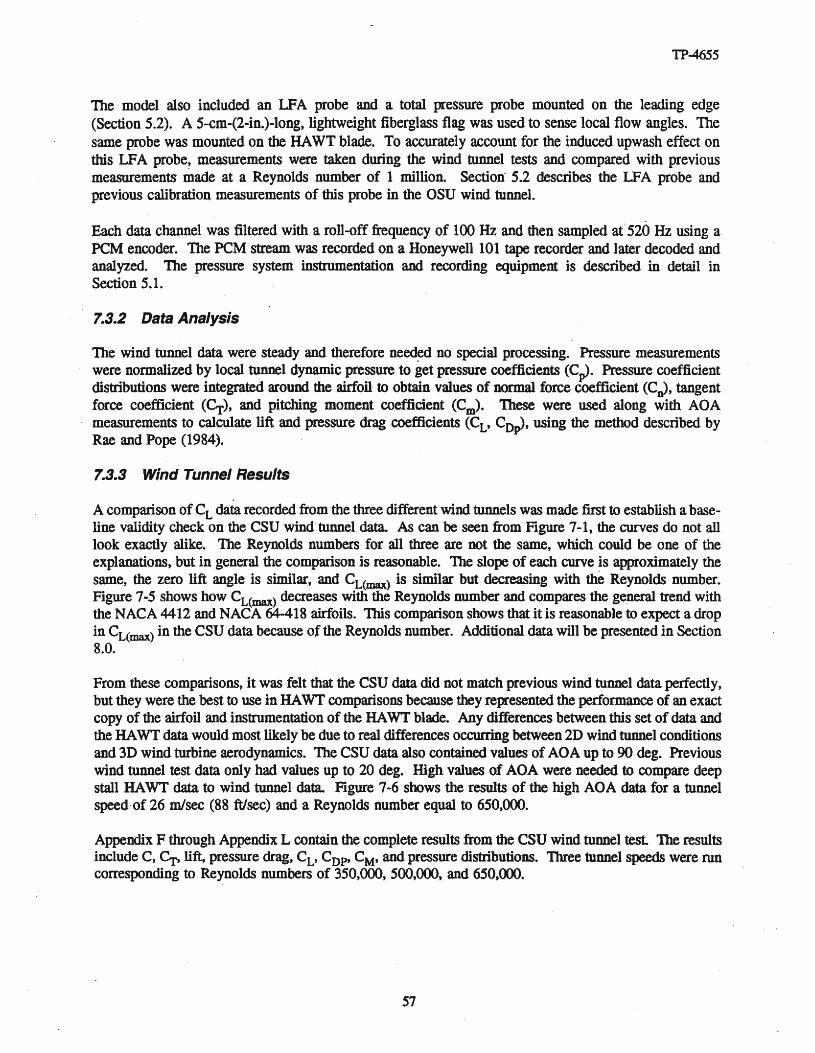
TP-4655
The model also included an LFA probe and a total pressure probe mounted on the leading edge(Section 5.2). A 5-cm-(2-in.)-long, lightweight fiberglass flag was used to sense local flow angles. Thesame probe was mounted on the HAWT blade. To accurately account for the induced upwash effect onthis LFA probe, measurements were taken during the wind tunnel tests and compared with previousmeasurements made at a Reynolds number of 1 million. Section"5.2 describes the LFA probe andprevious calibration measurements of this probe in the OSU wind tunnel.
Each data channel was filtered with a roll-off frequency of 100 Hz and then sampled at'520 Hz using aPCM encoder. The PCM stream was recorded on a Honeywell 101 tape recorder and later decoded andanalyzed. The pressure system instrumentation and recording equipment is described in detail inSection 5.1.
7.3.2 Data Analysis
The wind tunnel data were steady and therefore needed no special processing. Pressure measurementswere normalizedby local tunnel dynamicpressure to get pressure coefficients (CP>. Pressure coefficientdistributions were integrated around the airfoil to obtain values of normal force coefficient (CJ, tangentforce coefficient (Cr), and pitching moment coefficient (Cm). These were used along with AOAmeasurements to calculate.lift and pressure drag coefficients (CL, Cop>, using the method described byRae and Pope (1984).
7.3.3 Wind Tunnel Results
A comparisonof CLdata recordedfrom the three differentwind tunnelswas made first to establisha baseline validity check on the CSU windtunnel data. As can be seen from Figure 7-1, the curves do not alllook exactly alike. The Reynolds numbers for all three are not the same, which could be one of theexplanations, but in general the-comparisonis reasonable. The slope of each curve is approximately thesame, the zero lift angle is similar, and CL(max) is similar but decreasing with ttW Reynolds number.Figure 7-5 shows how CL(max) decreases with the Reynolds number and compares the general trend withthe NACA4412 and NACA 64-418 airfoils. This comparisonshowsthat it is reasonable to expect a dropin CL(max) in the CSU data because of the Reynoldsnumber. Additional data will be presentedin Section8.0.
From these comparisons, it was felt that the CSU data did not match previous wind tunnel data perfectly,but they were the best to use in HAWT comparisons because theyrepresentedthe performance of an exactcopy of the airfoil and instrumentation of the HAWT blade. Any differences betweenthis set of data andthe HAWT data wouldmost likely be due to real differences occurring between2D windtunnel conditionsand 3D wind turbine aerodynamics. The CSU data also containedvalues of AOA up to 90 deg. Previouswind tunnel test data only had values up to 20 deg. High values of AOA were needed to compare deepstall HAWT data to wind tunnel data. Figure 7-6 shows the results of the high AOA data for a tunnelspeed-of 26 mlsec (88 ftIsec) and a Reynolds number equal to 650,000.
Appendix F through Appendix L contain the completeresults from the CSU wind tunnel test The resultsinclude C, C1" lift, pressure drag, CL, CDP' CM, and pressuredistributions. 'Three tunnel speeds were runcorresponding to Reynolds numbers of 350,000, 500,000, and 650,000.
57
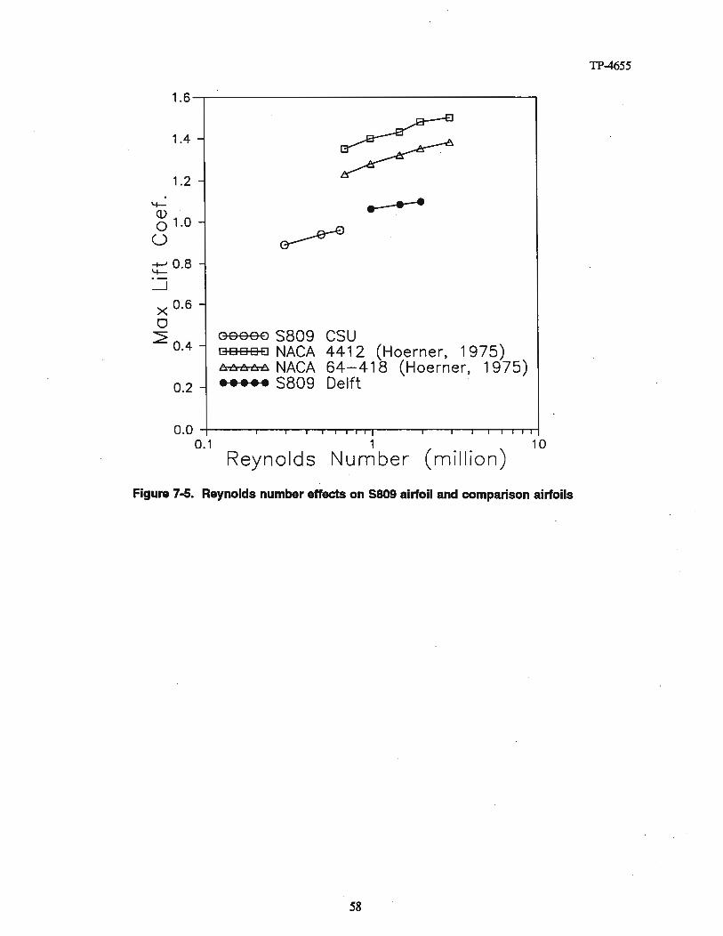

TP-4655
8.0 Rough Airfoil Performance Tests
8.1 Background
Blade surfaceroughness has been observed to decrease the efficiency of stall-controlled windturbines byas much as 40% (Yekutieli and Clark, 1987). Most of the degradation can typically be attributed topremature stalling of the airfoil, which lowers the maximum lift coefficient Figure 8-1 illustrates theeffect this can have on stall-controlled rotors. It shows a dramatic difference in the peak powerperformance for an Enertech 6Q-kW wind turbine before and after a rain shower. A smaller decline inrotor performance caused by leading edge roughness is experienced at lower AOAs, which can be asignificant factor in determining energy capture for pitch-controlled wind turbines (Holtz, 1988).
70.---------------------,
60
50
o'([0-00,.
C? C!.9 C!.9 Clean Blades .;0~Unclean Blades 0"0•
9'?
2018
o
8 10 12 14 16Wind Speed (m/s)
l'r?
d/
QlD °/
6O-+----r--~-__r--.___-_._-__r--.,._---i
4
10
20
L..(l)
~ 30o0...
Figure 8-1. 6o-kilowatt HAWT performance
Leading edge roughness on wind turbine blades is a universal problem that affects virtually everyconfiguration of wind turbine. It has contributed significantly to producing lower energy, fouling windturbine control algorithms, and making loads more difficult to predict Traditional airfoils, such as theNACA44XXor 23XXX, are beingdiscarded by wind turbinebladedesigners as they becomemore awareof the high degree of roughness sensitivity that these airfoils have. Newer airfoil designs such as theNREL airfoil families and the LS-l series from the National Aeronautics and Space Administration arebecoming more popular largely because of their relative insensitivity to roughness.
The effectsof roughness on airfoils are most commonly inferredby examining the influence on the rotor'spower curve. This method is accurate and reliable for determining the impact on energy capture for a
60
TP4655
specific HAWT configuration, but it does not provide much information about changes to the aerodynamicproperties of the airfoil. Wind tunnel tests may be used to predict performance degradations caused byroughness in the sub-stall regions, but stalled airfoil behavior is radically different on a rotating blade.The problem is that the stalled airfoil performance on a rotating wing is modified by 3D flow effects(Madsen, Rasmussen, and Pedersen, 1988). It is common for wind turbine designers to underestimatepeak performance and loads using wind tunnel airfoil data. Measurements taken directly off the rotatingairfoil are the only accurate way to completely determine the effect of roughness on airfoil properties.
8.2 Roughness Description
Most airfoil roughness problems experienced by HAWTs have been caused primarily by insectsaccumulating on the surface near the leading edge of the blade. The distribution is generally non-uniform,with larger particle sizes and particle densities distributed near the leading edge, rapidly declining towardthe trailing edge. In general, particle size usually increases and particle density decreases whenprogressing from the tip toward the root 'of the blade.
The NACA standard roughness was created to simulate the typical roughness distribution experienced byaircraft, This standard consists of a uniform distribution of particles between the leading edge and the 8%chord line on the upper and lower surfaces of the airfoil (Bragg and Gregorek, 1989). Particle size isdefined by the non-dimensional ratio of the particle diameter (k) divided by the chord length (c). The k1cvalue for the NACA standard roughness is .00046, which corresponds to grit sizes of .21 mm (.0083 in.)for the Combined Experiment rotor.
Operating conditions for wind turbines are quite different than for aircraft, however. Wind turbinesoperate closer to the ground and at lower Reynolds numbers and are cleaned less frequently.Consequently, the NACA standard roughness is not severe enough to represent the actual accumulationof insects observed by the authors. In order to do a realistic test of rough airfoil performance on the S809,it was necessary to create a roughness Pattern that was more appropriate for wind turbine applications.
A "simulated insect" roughness was developed and applied to all three blades over the outer 3.35 m(11 fi). Coarse grit particles ranging in size from 0.5 to 1.0 mm (.020 to .040 in.) were distributed ontoa 20.3-cm-wide (8-in.) strip of 3M #444 double-coated tape, 0.05-mm thick, that was centered on theleading edges of each blade. The grit was scattered randomly by dropping it onto the leading edge tapefrom above while the blade was horizontal with the leading edge positioned upward This created gritpatterns of.varying density that approximated the natural accumulation of insects and dirt on the blades.Grit densities were highest at the leading edge where 62 particleslcm2 (400 particlesJin2.) were countedand dropped off to zero particles near the aft edge of the tape. A photograph of the roughness distributionused is shown in Figure 8-2. The resulting k1cvalues ranged from .0011 to .0022, or roughly 2 to 4 timesthe NACA standard roughness size. Although the grit densities tapered off toward the trailing edge, somegrit particles were scattered back as far as 20% chord
Particle size and placement on the low-pressure surface of the airfoil are the two leading factors indetermining the severity of roughness (Bragg and Gregorek, 1989). When compared to NACA standardroughness, the NREL roughness distribution was more severe. This was an important factor in comparingthe data from this test with other airfoil data.
61

TP-4655
Figure 8-2. Roughness distribution on leading edges of test turbine blades
8.3 Roughness Testing
All the wind turbine roughness testing was conducted during Phase I of the Combined Experiment inMay 1989. Windtunnel roughness tests were conducted at CSUin September 1989. Windturbine testswereconducted over windspeeds ranging from5 m1sec (11.2 mph) to 30 m1sec (67.1 mph). Rough rotordata of 3.5 h wererecorded. Electrical power, shafttorque, andnineprop-vane anemometer signals werethe primary signals used for the performance comparisons; however, the active pressure, bladeload, andinflow signals were used to determine the aerodynamic effects of roughness on the airfoil. Most of theanalysis and data reduction techniques used follow the procedures described in the previous sections, butsome small changes were introduced for simplicity. The interested reader is referred to Musial,Butterfield, and Jenks (1989) and Musial and Butterfield (1990).
8.4 Rough Performance Results
A fifth-order polynomial was fit through each data set of rough and smooth data to obtain an accurateevaluation of the roughrotorperformance effects. Thesecurves are compared in Figure8-3 from 5 m1sec(11.2 mph) to 22 m1sec (49.2mph). Bothcurves haveapproximately the sameShape, but the rough data
62

TP4655
25~----~-~---------------------,
_ _ Measured Rough Data ( Curve Fit ). Measured Smooth Data ( Curve Fit )IJ-&+oEHI PROPPC ( OSU Smooth wr Data )
20
353010 15 20 "25Wind Speed (m/s)
5O-t----~--___r---____.---....,._---.,...._--__..,.....---_1
o
L.G)
3:o 10(L
5
Figure 8-3. Combined experiment wind turbine performance
curve is about 10% lower than the smooth data curve for most of the low to moderate wind speeds. Atabout 15 mlsec (33.6 mph), the two curves converge, and at 19 mlsec (42.5 mph), they cross.
Another way to look at this degradation is shownin Figure 8-4, where two normalized power curvesareplotted on the same graph. Both are plots of rough rotor performance normalized against smooth rotorperformance for the range of windspeedstested. A valueof 1.0on this curve wouldindicate no effectivechange caused by roughness. The percent of degradation caused by roughness is greatest at low windspeedsfor these curves. As indicated, one curve is mechanical power, and one curveis electrical power.Because data for these two curves were measured using independent transducers, their agreement ispresented here to validate the accuracy of the measurement
In Figure 8-3, the measured roughand smoothmechanical powercurvesare also compared to a predictedpower curve that was generated using PROppe performance code with 2D lift and drag data. Liftcoefficients from the OSU wind tunnel tests that were used to generate the predicted power curve areshown in Figure 8-5. The smooth measured data match the analytical predictions very closely untilapproximately 15 m1sec (33.6 mph), where the analytical power curves reach a maximum value at about15 kW and begin to roll off. The measured smooth power curve continues to increase beyond 18 kWwithout leveling off. At low wind speeds below 15 mlsec (33.6 mph), the smooth, predicted curvesexceed the rough data, as expected. As seen previously in Figure 8-4, the rotor experiences an average
63

TP-4655
1.1
~
(1) 1.03:o
0..0.9
...c+-'oE0.8
(f)<,~ 0.7(1)
3:o
0.. 0.6
.....---------------------K
...c01::J 0.5o
0:::
...- - Generator Power• • • • • Mechanical Power
0.4
25.0010.00 15.00 20.00Windspeed M/S -
0.3 -t-----.------r--------,.-------15.00
Figure 8-4. Normalized power output--combined experiment
decline of 10% in power production because of the leading edge roughness, but the rough and smoothmeasured power curves diverge from the predicted curve and continue to increase without reaching anupperlimit. 'This is a familiar problem that relates to the stall characteristics of windturbines ratherthana roughness phenomenon. '
The effects of roughness on the Combined Experiment windturbine were examined aboveby comparingroughand smooth powercurves. It is clearthat roughness had a negative effectoilperformance overmostof the operating range, but this rotor did not experience the drop-offin peak power that is usually seenon stall-controlled rotors. It was not clear what caused this effect.
'This windturbine differs from mostcommercial stall control windturbines because of its constant chord,zero-twist rotor. Therefore, muchof the inboard sections of the rotor operate in the stall region even atlow to moderate wind speeds. Much of the peak power performance is dictated by the deep stallcharacteristics of the airfoil and not by the low AOA section properties (AOA = 0-10 deg). In order tounderstand what is happening on this rotor, it is necessary to look at the stalled airfoil properties.
8.5 Rough 5809 Airfoil Characteristics
To studythe effectof roughness on airfoil properties, aerodynamic pressure measurements taken at 80%span were used. Figure 8-6 shows the rough and smooth C1 versus AOA curves for the rotating (windturbine) and non-rotating (wind tunnel) cases out to 25-deg AOA. All four curves are in goodagreementfor very low AOA (0-3 deg). At 3 deg the roughdata for both the 2D and 3D casesbeginto drop off
64
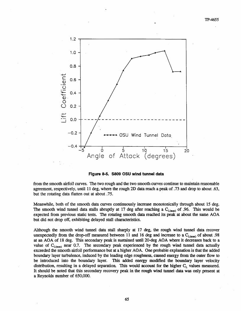
TP-4655
1.2 -r------------------------.
205 10 15
of Attack (degrees)
.......... OSU Wind Tunnel Data
-0.4 T-.;t----...----r------r---~---~-5 0
Angle
-0.2
-+-JC(1) 0.6
U
:::= 0.4(1) .
· 0U 0.2
1.0
0.8
Figure 8-6. S809 OSU wind tunnel data
from the smooth airfoil curves. The two rough and the two smooth curves continue to maintain reasonableagreement, respectively, until 11 deg, where the rough 2D datareach a peak of .73 and drop to about .63,but the rotating data flatten out at about .75.
Meanwhile, both of the smooth data curves continuously increase monotonically through about 15 deg.The smooth wind tunnel data stalls abruptly at 17 deg after reaching a CL(mu) of .96. This would beexpected from previous static tests. The rotating smooth data reached its peak at about the same AOAbut did not drop off, exhibiting delayed stall characteristics.
Although the smooth wind tunnel data stall sharply at 17 degt the rough wind tunnel data recoverunexpectedly from the drop-off measured between 11 and 16 deg and increase to a CL(mu) of about .98at an AOA of 18 deg. This secondary peak is sustained until 2O-deg AOA where it decreases back to avalue of CL(mu) near 0.7. The secondary peak experienced by the rough wind tunnel data actuallyexceeded the smooth airfoil performance but at a higher AOA. One probable explanation is that the addedboundary layer turbulence, induced by the leading edge roughness, caused energy from the outer flow tobe introduced into the boundary layer. This added energy modified the boundary layer velocitydistribution, resulting in a delayed separation. This would account for the higher CL values measuredIt should be noted that this secondary recovery peak in the rough wind tunnel data was only present ata Reynolds number of 650,000.
65
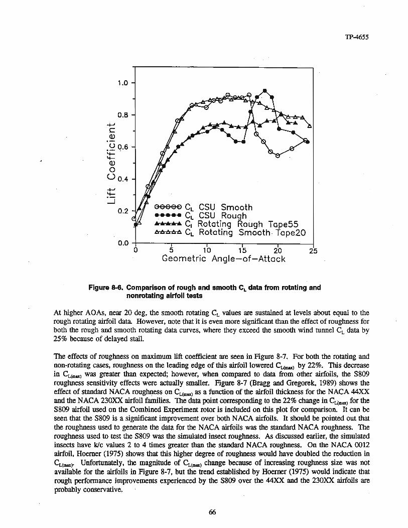
TP-4655
1.0
0.8-+.-JCQ).-
.U q.6'+'+-Q)
oUO.4
-+-''+-~
0.2 00000 CL CSU Smooth••••• CL CSU Rough......... C, Rotating Rough Tape55.t&AAAA CL Rotating Smooth Tape20
0.0 +-----,.---.----,.---..,...-----lo 5 10 15 20
Geometric Angle-of-Attack25
Figure 8-6. Comparison of rough and smooth CL data from rotating andnonrotating airfoil tests
At higher AOAs, near 20 deg, the smooth rotating CLvalues are sustained at levels about equal to therough rotating airfoil data. However, note that it is even moresignificant than the effectof roughness forboth the rough and smooth rotating data curves, where they exceed the smooth wind runnel CLdata by25% because of delayed stall.
The effects of roughness on maximum lift coefficient are seen in Figure 8-7. For both the rotating andnon-rotating cases, roughness on the leading edge of this airfoil lowered CL(III8lt) by 22%. This decreasein CL(mu) was greater than expected; however, when compared to data from other airfoils, the S809roughness sensitivity effects were actually smaller. Figure 8-7 (Bragg and Gregorek, 1989) shows theeffect of standardNACAroughness on CL(mu) as a function of the airfoil thickness for the NACA44XXand the NACA230XXairfoil families. The data point corresponding to the 22% changein CL(mu) for theS809 airfoil used on the Combined Experiment rotor is included on this plot for comparison. It can beseen that the S809 is a significant improvement over both NACA airfoils. It should be pointed out thatthe roughness used to generate the data for the NACA airfoils was the standard NACA roughness. Theroughness used to test the S809 was the simulated insect roughness. As discussed earlier, the simulatedinsects have klc values 2 to 4 times greater than the standard NACA roughness. On the NACA 0012airfoil, Hoerner (1975) shows that this higher degree of roughness wouldhave doubled the reduction inCL(mu). Unfortunately, the magnitude of CL(mu) change because of increasing roughness size was notavailable for the airfoils in Figure 8-7, but the trend established by Hoerner (1975) would indicate thatrough performance improvements experienced by the S809 over the 44XX and the 230XX airfoils areprobably conservative.
66
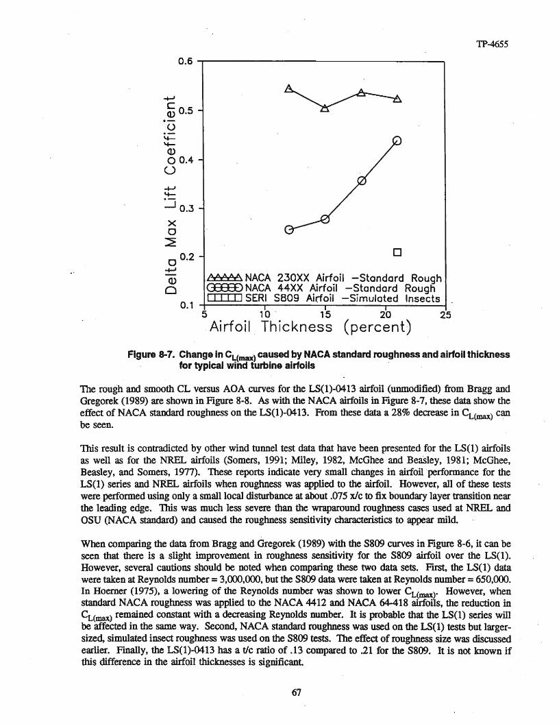
TP-4655
0.6 ~-------------------
-+-'cQ) 0.5
e_
U'+-'+-Q)00.4
U.......,'+-
:..J 0.3
Xo~
0°·2-+-'Q)
o0.1
o
AAAAA. NACA 230XX Airfoil -Standard Rougha:a::E> NACA 44XX Airfoil -Standard RoughI I I I I I SERI S809 Airloil -Simulated Insects
5 10 . 15 20 25
.Airfoil Thickness (percent)
Figure 8-7. Change in CL(max) caused by NACA standard roughness and airfoil thickness. for typical wind turbine airfoils .
The rough and smooth CL versus AOA curves for the LS(I)-0413 airfoil (unmodified) from Bragg andGregorek (1989) are shown in Figure 8-8. As with the NACA airfoils in Figure 8-7, these data show theeffect of NACA standard roughness on the LS(l)-0413. From these data a 28% decrease in CL(max) canbe seen.
'This result is contradicted by other wind tunnel test data that have been presented for the LS(l) airfoilsas well as for the NREL airfoils (Somers, 1991; Miley, 1982, McGhee and Beasley, 1981; McGhee,Beasley, and Somers, 1977). These reports indicate very small changes in airfoilperformance for theLS(1) series and NIffiL airfoils when roughness was applied to the airfoil. However, all of these testswere performed using only a smalllocaI disturbance at about .075 xJc to fix boundary layer transition nearthe leading edge. This was much less severe than the wraparound roughness cases used at NREL andOSU (NACA standard) and caused the roughness sensitivity characteristics to appear mild.
When comparing the data from Bragg and Gregorek (1989) with the S809 curves in Figure 8-6, it can beseen that there is a slight improvement in roughness sensitivity for the S809 airfoil over the LS(l).However, several cautions should be noted when comparing these two data sets. FlI'St, the LS(I) datawere taken at Reynolds number =3,000,000, but the S809 datawere taken at Reynolds number =650,000.In Hoerner (1975), a lowering of the Reynolds number was shown to lower CL(max). However, whenstandard NACA roughness was applied to the NACA 4412 and NACA 64-418 airfoils, the reduction inCL(max) remained constant with a decreasing Reynolds number. It is probable that the LS(I) series willbe affected in the same way. Second, NACA standard roughness was used on the LS(l) tests but largersized, simulated insect roughness was used on the S809 tests. The effect of roughness size was discussedearlier. Finally, the LS(l)-0413 has a tic ratio of .13 compared to .21 for the S809. It is not known ifthis difference in the airfoil thicknesses is significant
67
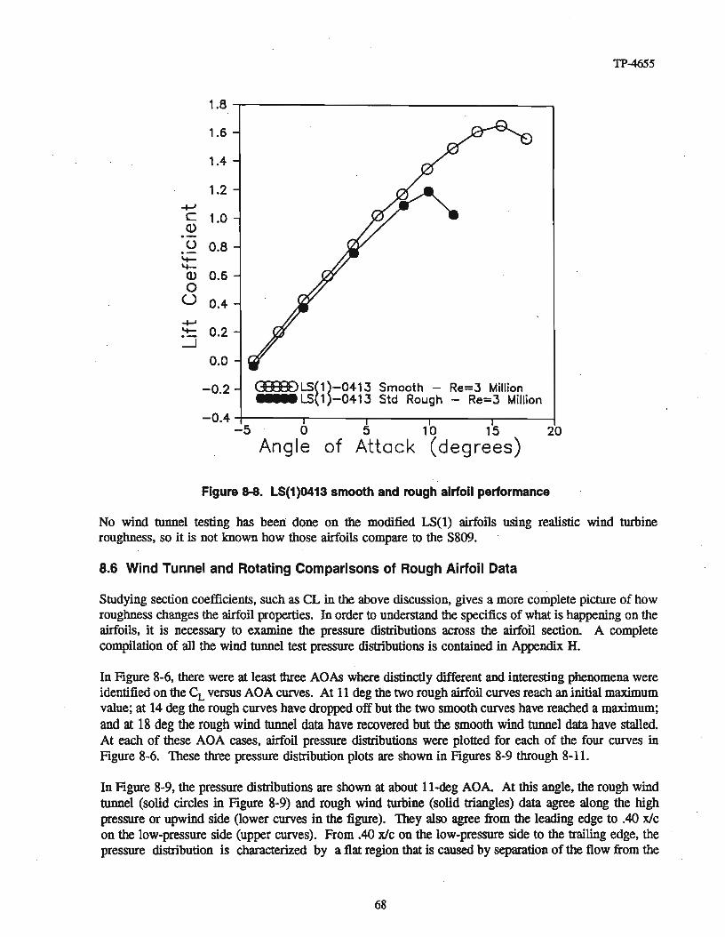
TP-4655
1.8
1.6
1.4
1.2-+oJc 1.0Q).-0 0.8.-
'+-'+-Q) 0.60
U 0.4-+oJ'+- 0.2:....J
0.0
-0.2 (m:!)LS(1)-0413 Smooth - Re=3 MillionI •••• LS(1)-0413 Std Rough - Re=3 Million
205 10 15of Attack (deg rees)
-0.4 ;-----r----,-----r---.-------I-5
Figure 8-8. LS(1)0413 smooth and rough airfoil performance
No wind tunnel testing has been done on the modified LS(l) airfoils using realistic wind turbineroughness, so it is not known how those airfoils compare to the S809.
8.6 Wind Tunnel and Rotating Comparisons of Rough Airfoil Data
Studying sectioncoefficients, such as CL in the abovediscussion, gives a more complete pictureof howroughness changes the airfoil properties. In order to understand the specifics of what is happening on theairfoils, it is necessary to examine the pressure distributions across the airfoil section. A completecompilation of all the wind tunnel test pressure distributions is contained in Appendix H.
In Figure 8-6, there were at least three ADAs wheredistinctly different and interesting phenomena wereidentified on the CL versusADA curves. At 11 degthe two roughairfoil curvesreach an initial maximumvalue; at 14 deg the rough curveshave droppedoff but the two smoothcurveshave reacheda maximum;and at 18 deg the rough wind tunnel data have recovered but the smooth wind tunnel data have stalled.At each of these ADA cases, airfoil pressure distributions were plotted for each of the four curves inFigure 8-6. These three pressure distribution plots are shown in Figures 8-9 through 8-11.
In Figure 8-9, the pressuredistributions are shown at about ll-deg ADA. At this angle, the rough windtunnel (solid circles in Figure 8-9) and rough wind turbine (solid triangles) data agree along the highpressure or upwind side (lower curves in the figure). 1bey also agree from the leading edge to .40 x1con the low-pressure side (upper curves). From.4O x1c on the low-pressure side to the trailing edge, thepressure distribution is characterized by a flat regionthat is causedby separation of the flow from the
68


TP-4655
-4-,----------------------,
-3...cQ)
o~ -2Q)
oU
Q)~
::J -1en(J)Q)L.-n,
o
10.0
G8E3E3E) CSU WT - Smooth 18.0 Deg C1=0.639••••• CSU WT - Rough 18.1 Deg C.=O.956.A•••• HAWT - Rough 18.5 Deg C.=O.77••••• HAWT - Smooth 18.5 Deg C1=0.849
0.2 0.4 0.6 0.8Blade Chord X/C
1.0
Figure 8-11. A comparison of pressure distributions for 180 angle of attack
airfoil. On close examination, one can see that the rough wind turbine pressure data meet that flat regionabout .10 xlc further toward the trailing edge than the non-rotating case. This implies that slightly delayedseparation may result from blade rotation.
Both smooth curves (open symbols) in Figure 8-9 show significantly lower (i.e., higher negative) pressuresin the low-pressure, leading edge region. Again, the rotating wind turbine blade data show a delayedseparation when compared to the wind tunnel data. The lower pressures in the leading edge region onthe smooth airfoils caused higher smooth lift coefficients. Both smooth curves resulted in CLs that were25% higher than the rough cases (see legend in Figure 8-9 for values of Cr).
Figure 8-10 shows pressure distributions for 14-deg AOA. Here, a larger difference in leading suctionpeak and separation point can be seen. The smooth curves show a Cp of -4.3 and -4.8 for the rotatingblade and the wind tunnel, respectively. Both rough cases show a maximum negative peak Cp of -3.3.Again, the separation point was delayed about .10 xlc for the rotating blade cases over their respectivewind tunnel cases. As would be predicted from Figure 8-6, both smooth cases show higher negativepressures over the first half of the low-pressure side of the airfoil. This difference is due to attached flowextending further toward the trailing edge for the smooth cases. For the wind tunnel cases, this resultedin a CL that was 40% greater for the smooth case than the rough case. For the rotating cases, thedifference between rough and smooth CL was only 25%.
At 18-deg AOA (Figure 8-11), the smooth wind tunnel data show a complete loss of suction peak. Thedistribution of pressures on the low-pressure side of the airfoil is nearly flat from the leading edge to thetrailing edge. This is caused by complete flow separation starting at the leading edge.
70

TP-4655
On the other three curves, high, negative pressures associated with high-velocity attached flow are evident.The rough wind tunnel data still show a strong suction peak, explaining the high CL at 18 deg inFigure 8-6. Now, CL for the rough case is 49% higher than the smooth case. It is probable thatturbulence resulting from roughness at the leading. edge has caused energy from the outer flow to beintroduced into the inner boundary layer flow at this Reynolds number. This energy modified theboundary layer velocity profile, making it similar to the effect of a vortex generator. The modifiedvelocity profile appears to have delayed flow separation and maintained the pressure peak at the leadingedge well beyond the normal stall angle.
. For the smooth rotating blade, the separation point appears to be further aft than the rough rotating case,but no sharp transition from attached flow (decreasing pressures) to separated flow (flat pressures) isvisible in these curves. This may be an anomaly of the averaging process, or it may be caused by 3Drotational effects. Further research is under way that is targeted at understanding the rotational andunsteady effects of these pressure measurements and will be the subject of future reports.
Further efforts to quantify the differences in roughness sensitivity between LS(1) and the NREL airfoilsshould be made using the same roughness conditions under similar conditions. It is important that arealistic roughness distribution, appropriate for wind turbines, be used in these experiments.
71

TP-4655
9.0 References
Akins, R E., 1987, Evaluation of SERUPSC Pressure System (Unpublished), NREL, Golden, CO.
APEX Systems, Inc., 1988, PCM Decoder Card Manual, APEX Systems, Inc., Boulder, CO.
Bendat, 1. S., and Piersol, A. G., 1980, Engineering Applications of Correlation and Spectral Analysis,A Wiley-Interscience Publication, John Wiley & Sons, New York.
Bragg, M. B., and Gregorek, G. M., 1989, "Environmentally Induced Surface Roughness Effects onLaminar Flow Airfoils: Irilplications for Flight Safety," Proceedings ofAIAA, Aircraft Design, Systemsand Operations Conference, Seattle, WA, July 31-Aug. 2, 1989, published by AIAA, 370 L'EnfantPromenade, S.W., Washington, D.C. 20004.
Butterfield, C. P., Scott, G. N., and Musial, W., 1990, Comparison of Wind Tunnel Airfoil PerformanceData with Wind Turbine Blade Data, 'IP-254-3799, NREL, Golden, CO.
Butterfield, C. P., 1989b, Three-Dimensional Airfoil Performance Measurements on a Rotating Wing,'IP-217-3505, NREL, Golden, CO.
Butterfield, C. P., Jenks, M. D., Simms, D. A., and Musial, W. P., 1990, Aerodynamic PressureMeasurements on a Rotating Wind Turbine Blade, 'IP-257-3695, NREL, Golden, CO.
Butterfield, C. P., 1989a, "Aerodynamic Pressure and Flow Visualization Measurements from a RotatingWind Turbine Blade," Proceedings of the Eighth ASME Wind Energy Symposium, Houston, TX,January 22-25, 1989, Vol. 7, pp. 245-255.
Butterfield, C. P., and Nelson, E. N., 1990, Aerodynamic Testing of a Rotating Wind Turbine Blade,'IP-257-3490, NREL, Golden, CO.
Fairchild Weston Systems, Inc., 1985, PCM Data Collection and Reduction System for the Solar EnergyResearch Institute: Operating Manual, Fairchild Weston Systems, Inc., Sarasota, FL.
Gregorek, G. M., Hoffman, M. J., and Mulh, K.. E., 1991, Wind Tunnel Tests of the S809 Airfoil Model,NREL, Golden, CO.
Hoerner, S. F., 1975, Fluid-Dynamic lift. Hoerner Fluid Dynamics, Brick Town, NJ.
Holtz, R., 1988, "The Effect of Blade Surface Roughness on the Lead-Lag Bending Moments of a U.S.Windpower 56-100 Wind Turbine," Proceedings of the Seventh ASME Wind Energy Symposium,American Society of Mechanical Engineers, New Orleans, Louisiana, Jan. 10-13, 1988, pp. 95-99.
Irwin, H., Cooper, K. R, and Hirard, R, 1979, "Correction of Distortion Effects Caused by TubingSystems in Measurements of Fluctuating Pressures," Journal ofIndustrial Aerodynamics 5, pp. 93-107.
Lenschow, D. H., 1971, "Vanes for Sensing Incidence Angles of the Air from an Aircraft," Journal ofApplied Meteorology, Vol. 10, No.6, pp. 1339-1343. .
72
TP-4655
Lora! Instrumentation, DIPAD Mark II Manual, Loral Instrumentation, San Diego, CA.
Madsen, H. A., Rasmussen, F., and Pedersen, T. F., 1988, Aerodynamics ofa Full-Scale HAWT Blade,Riso National Laboratory, Roskilde, Denmark.
McGhee, R. J., Beasley, W. D., and Somers, D. M., 1977, Low-Speed Aerodynamic Characteristics of a13-Percent-Thick Airfoil Section Designed for General Aviation Applications, NASA TM X-72697,Langley Research Center, Hampton, VA.
McGhee, R. J., and Beasley, W. D., 1981, Wind Tunnel Results for a Modified 17-Percent Thick LowSpeed Airfoil Section, Technical Paper 1919, National Aeronautics and Space Administration, Houston,TX.
Miley S. J., 1982, A Catalog ofLow Reynolds Number Airfoil Data for Wind Turbine Applications, RFP3387, U.S. Department of Energy, Washington, D.C.
Musial, W. D., Butterfield C. P., and Jenks, MD., 1989, Effects ofLeading-edge Roughness on S809Airfoil Rotor Performance, TP-217-3563, NREL, Golden, CO.
Musial, W., and Butterfield, C. P., 1990, A Comparison of Two- and Three- Dimensional S809 AirfoilProperties for Rough and Smooth HAWT Rotor Operation, TP-257-3603, NREL, Golden, CO.
Rae, H. W., and Pope, A., 1984, Low-Speed Wind Tunnel Testing, Second Edition, John Wiley & Sons,New York.
Rae, W. H., Jr., and Pope, A., 1984, Low-Speed Wind Tunnel Testing, Second Edition, John Wiley &Sons, New York, p. 133.
Simms, D. A., and Butterfield, C. P., 1990, Unsteady Aero Experiment "[est Plan (Unpublished), NREL,Golden, CO.
Simms, D. A., 1990, PC-Based PCM Telemetry Data Reduction System Software, '):P-257-3663, NREL,Golden, CO.
Simms, D. A., and Butterfield, C. P., 1990, PC-Based PCM Telemetry Data Reduction System Hardware,TP-257-3662, NREL, Golden, CO.
Somers, D. M, 1989, Design and Experimental Results for the S809 .Airfoil (Unpublished), NREL,Golden, CO.
Somers, D. M., 1991, Design and Experimental Results for the S809 Airfoil, NREL report, to bepublished
Strock, O. J., 1983, Telemetry Computer Systems: An Introduction, Prentice-Hall, Inc., Englewood Cliffs,NJ. -
Tangler, J. L., 1983, Horizontal-Axis Wind System Rotor Performance Model Comparison - ACompendium, RFP-3508, Rockwell International.
73
TP-4655
Vitema, L. A., and Corrigan, R. D., 1981, "Fixed Pitch Rotor Performance ofLarge Horizontal Axis WindTurbines," DOEJNASA Workshop on Large Horizontal Axis Wind Turbines, Cleveland, OH, July 28-30. .
Yekutieli, 0., and Clark, R. N., 1987, "Influence of Blade Surface Roughness on the Performance ofWindTurbines," Proceedings of the Sixth ASME Wind Energy Symposium, pp. 181-187, American Societyof Mechanical Engineers, Dallas TX, Feb. 15-18, 1987.
74

Appendix A
Combined/Unsteady Aero ExperimentHigh and Low Cal Setups for PCM600
A-I
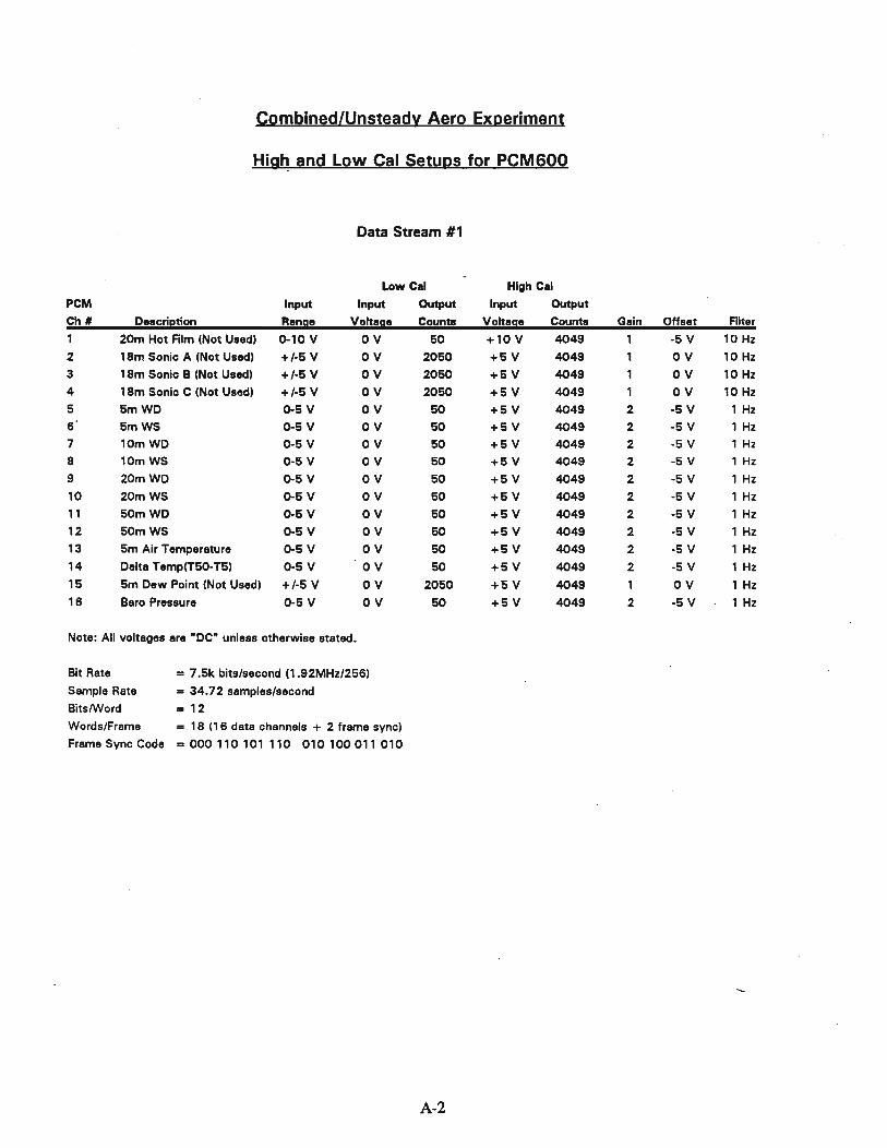
Combined/Unsteady Aero Experiment
Hig~ and Low Cal Setups for PCM600
Data Stream #1
Low Cal High Cal
PCM Input Input Output Input Output
Ch # Description Range Voltage Counts Voltage Counts Gain Offset Filter
1 20m Hot Film (Not Used) 0-10 V OV SO +10 V 4049 1 -S V 10 Hz
2 18m Sonic A (Not Used) +/-S V OV 20S0 +S V 4049 1 OV 10 Hz
3 18m Sonic B (Not Used) +/-S V OV 20S0 +S V 4049 1 OV 10 Hz
4 18m Sonic C (Not Used) +/-S V OV 20S0 +S V 4049 1 OV 10 Hz
S SmWD O-SV OV SO +S V 4049 2 -S V 1 Hz
6 SmWS O-S V OV SO +S V 4049 2 -S V 1 Hz
7 10mWD O-S V OV SO +S V 4049 2 -S V 1 Hz
8 10mWS O-SV OV SO +S V 4049 2 -S V 1 Hz
9 20mWD O-S V OV SO +S V 4049 2 -S V 1 Hz
10 20mWS O-SV OV SO +S V 4049 2 -S V 1 Hz
11 SOmWD O-S V OV SO +S V 4049 2 -S V 1 Hz
12 SOmWS O-SV OV SO +S V 4049 2 -S V 1 Hz
13 Sm Air Tempereture 0-5 V OV SO +S V 4049 2 -S V 1 Hz
14 Delta Temp(TSO-TS) O-S V OV SO +S V 4049 2 -S V 1 Hz
lS Sm Dew Point (Not Used) +/-S V OV 20S0 +SV 4049 1 OV 1 Hz
16 Baro Pressure O-S V OV SO +S V 4049 2 -S V 1 Hz
Note: All voltages are RDCRunless otherwise stated.
Bit Rate = 7.Sk bits/second (1.92MHz/2S6)
Sample Rate = 34.72 samples/second
BitslWord = 12Words/Frame = 18 (16 data channels + 2 frame sync)
Frame Sync Code = 000 110 101110 010 100011 010
A-2

Combined/Unsteady Aero -Experiment
High and low Cal Setups for PCM600
Data Stream #2
Low C.I High C.I
PCM Input Input Output Input Output
Ch # Description Range Voltage Counts Voltase Counts Gain Offset Filter
1 Propvane Anem. WS1 0-10 V OV 50 +10 V 4049 1 -5 V 2 Hz
2 Propvane Anem. WS2 0-10 V OV 50 +10 V 4049 1 -5 V 2 Hz
3 Propvane Anem. WS3 0-10 V OV 50 +10 V 4049 1 -5 V 2 Hz
4 Propvene Anem. WS4 0-10 V OV 50 +10 V 4049 1 -5 V 2 Hz
5 Propvane Anem. WS5 0-10 V OV 50 +10 V 4049 1 -5 V 2 Hz
6 Propvane Anem. WS6 0-10 V OV 50 +10 V 4049 1 -5 V 2 Hz
7 Propvane Anem. WS7 0-10 V OV 50 +10 V 4049 1 -5 V 2 Hz
8 Propvene Anem •.WS8 0-10 V OV 50 +10 V 4049 1 -5 V 2 Hz
9 Propvane Anem. WS9 0-10 V OV 50 +10 V 4049 1 -5 V 2 Hz
10 Propvane Anem. W09 0-10 V OV 50 +10 V 4049 1 -5 V 2 Hz
11 Bivane WS12 0-10 V OV 50 +10 V 4049 1 -5 V 2 Hz
12 Bivane WD12 0-2 V OV 50 +2.5V 4049 4 -5 V 2 Hz
13 Bivane WE12 0-2 V OV 50 +2.5V 4049 4 -5 V 2 Hz
14 Bivane WS13 0-10 V OV 50 +10 V 4049 1 -5 V 2 Hz
15 Bivane WD13 0-2 V OV 50 +2.5V 4049 4 -5 V 2 Hz
16 Bivane WE13 0-2 V OV 50 +2.5 V 4049 4 -5 V 2 Hz
Note: All voltages are "DC" u,nless otherwise stated.
Bit Rate ZI 15k bits/second (1.92MHz/128)
Sample Rate = 69.44 samples/second
BitslWord = 12Words/Frame = 18 (16 data channels + 2 frame sync)
Frame Sync Code = 000 110 101 110 010 100011 010
A-3
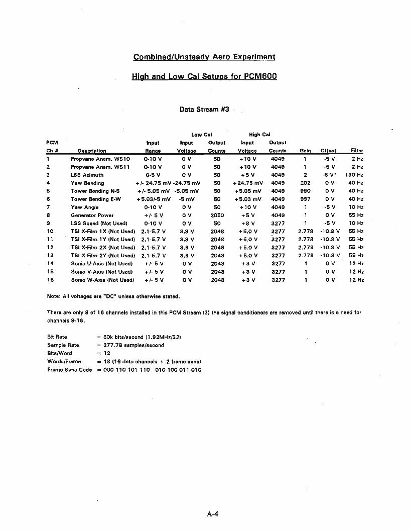
Combined/Unsteady Aero Experiment
High and Low Cal Setups for PCM600
Data Stream #3 '
Low Cal High Cal
PCM Input Input Output Input Output
Ch # Description Range Voltage Counts Voltase Counts Gain Offset Filter
1 Propvane Anem. WS10 0-10V OV 50 +10 V 4049 1 -5 V 2 Hz
2 Propvane Anem. WS11 Q.l0 V OV 50 +10 V 4049 1 -5 V 2 Hz
3 LSS Azimuth 0-5 V OV 50 +5V 4049 2 -5 V· 130 Hz
4 Yaw Bending +/- 24.75 mV -24.75 mV 50 +24.75 mV 4049 202 OV 40 Hz
5 Tower Bending N-S +/- 5.05 mV -5.05 mV 50 +5.05 mV 4049 990 OV 40 Hz
6 Towar Bending E-W +5.03/-5 mV -5 mV '50 +5.03 mV 4049 997 OV 40 Hz
7 Yaw Angle 0-10 V OV 50 +10 V 4049 1 -5 V 10 Hz
8 Generator Power +/- 5 V OV 2050 +5 V 4049 1 OV 55 Hz
9 LSS Speed (Not Used) 0-10 V OV 50 +8 V 3277 1 -5 V 10 Hz
10 TSI X-Film 1X (Not Used) 2.1-5.7 V 3.9 V 2048 +5.0 V 3277 2.778 -10.8 V 55 Hz
11 TSI X-Film 1Y (Not Used) 2.1-5.7 V 3.9 V 2048 +5.0V 3277 2.778 -10.8 V ·55 Hz
12 TSI X-Film 2X (Not Used) 2.1-5.7 V 3.9 V 2048 +5.0 V 3277 2.778 -10.8 V 55 Hz
13 TSI X-Film 2Y (Not Used) 2.1-5.7 V 3.9 V 2048 +5.0 V 3277 2.778 -10.8 V 55 Hz
14 Sonic U-Axis (Not Used) +/- 5 V OV 2048 +3 V 3277 1 OV 12 Hz
15 Sonic V-Axis (Not Used) +/- 5 V OV 2048 +3 V 3277 1 OV 12 Hz
16 Sonic W-Axis (Not Used) +/- 5 V OV 2048 +3 V 3277 1 OV 12 Hz
Note: All voltages are wDC· unless otherwise stated.
There ere onlv 8 of 16 channels installed in this PCM Stream (3) the signal conditioners are removed until there is a need for
channels 9-16.
Bit Rate
Sample Rate
BitslWord
Words/Frame
Frame Sync Code
:: 60k bits/second (1.92MHz/321
:: 277.78 samples/second
:: 12
= 18 (16 data channels + 2 frame sync)
= 000 110 101 110 010 100011 010
A-4

Combined/Unsteady Aero Experiment
High and Low Cal Setups for PCM600
Data Stream #4
Low C.I High C.I
PCM Input Input Output Input Output
Ch # Description Range Voltage Counts Voltage Counts Gain Offset Filter
1 Root Flap "RTFBM-A" ±6.25 mV OV 2048 800 OV 40 Hz
2 Root Flap "RTFBM-B" ±5.0 mV OV 2048 1000 OV 40 Hz
3 Root FI Blade 2 "RTFBM-2" ±5.0 mV OV 2048 1000 OV 40 Hz
4 Root Fl Blade 3 "RTFBM-3" ±6.25 mV OV 2048 800 OV 40 Hz
5 20% Flap "20FBM" ±5.0 mV OV 2048 1000 OV 40 Hz
6 40% Flap"4OFBM" ±10.0mV OV 2048 500 OV 40 Hz
7 50% Flap "50FBM" ±7.0 mV OV 2048 700 OV 40 Hz
8 60% Flap "60FBM" (Not Used) •
9 70% Flap "70FBM" ±S.O mV OV 2048 1000 OV 40 Hz
10 75% Flap "75FBM"(Not Used) -
11 80% Flap "80FBM" (Not Used) -
12 85% Flap "85FBM" (Not Used) -
13 90% Flap "90FBM" ±2.5 mV OV 2048 2000 OV 40 Hz14 Root Edge "RTEBM-A" ±6.2S mV OV 2048 800 OV 40 Hz15 20% Edge"20EBM" ·± 7.0 mV OV 2048 700 OV 40 Hz16 50% Edge"50EBM" ±10.0 mV OV 2048 500 OV 40 Hz
17 70% Blade Torque "70Ta" ± 2.5 mV OV 2048 2000 OV 40 Hz18 85% Edge "85EBM" (Not Used)-
19 Root Torque (Unk) "RTTa" ± 2.5 mV OV 2048 2000 OV 40 Hz
20 50% Torsion "SOTa" ±2.5 mV OV 2048 2000 OV 100 Hz
21 X-X LSS "LSSX-X" ± 10.0 mV OV 2048 500 OV 40 Hz
22 V-V LSS "LSSY-Y" ± 10.0 mV OV 2048 500 OV 40 Hz23 LSS Torque "LSSTa-A" ±5.0 mV OV 2048 1000 OV 40 Hz
24 LSS Torque "LSSTa-B" ±5.0 mV OV 2048 1000 OV 100 Hz25 85% RTD (Not Used)
26 Load Cell for Blade Pull Testing (Cal Only)
'27-58 Pressure Taps ±S.OV 1 OV 100 Hz
59 Absolute Pressure 0-5 V 2 :'5 V 1.5 kHz
60 Ca' Pressure ±2.5 V 2 OV 1.5 kHz
61 Pitch ·Angle 0-5 V 1 OV62 PCM Voltage Monitor 0-28 V .2 OV
Note: All voltages are "DC" unless otherwise stated.
Bit Rate ::II: 400k bits/second
Sample Rate = 520.83 samples/second
BitslWord = 12Words/Frame - 64 (62 data channels + 2 frame sync)
Frame Sync Code - 111110101 111 001 100 100000
A-5

Combined/Unsteady Aero Experiment
High and Low Cal Setups for PCM600
Data Stream #8
PCMCh#
1
23
4-62
DescriptionAbsolute PressureCal PressureSparePressure Taps
Input
Range0-5 V
±2.5 V
±5.0 V
Low Cal
Input Output
Voltage Counts
Data Stream #9
High Cal
Input OutputVoltage Counts Gain Offset Filter
2 -5 V 1.5 kHz
2 0 V 1.5 kHz
o V 100 Hz
PCMCh#1·3435
36
3738
39
40
4142-454647-52
53
54
55-62
DescriptionPressure Taps86% AOASpare
67.3% AOASpareSpareSpare
34% AOASpare
50.6% AOASpareAbsolute Pressure
Cal PressureSpare
InputRange±5.0 V
± 10.0 V
± 10.0 V
±10.0 V
± 10.0 V
0-5 V±2.5 V
Low Cal
Input OutputVoltage Counts
High Cal
Input OutputVoltage Counts Gain
1
2
2
Offset Filtero V 100 Hz
OV
OV
OV
OV
-5 V 1.5 kHz
o V 1.5 kHz
Note: All voltages are "DC" unless otherwise stated.
Bit Rate
Sample Rate
BitslWordWords/Frame
Frame Sync Code
= 400k bits/second
= 520.83 samples/second
= 12= 64 162 data channels + 2 frame sync)= 111110101111 001100100000
A-6
Appendix B
Unsteady Aero Experiment Measurement Tolerances
B-1
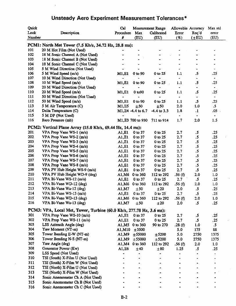
Unsteady Aero Experiment Measurement Tolerances *
Quick Cal Measurement Range Allowable Accuracy Max stdLook Description Procedure Max Calibrated Error Req'd errorNumber # (EU) (EU) (%) (±EU) (EU)
PCM1: North Met Tower (7.5 Kb/s, 34.72 Hz, 28.8 ms):101 20 M Hot Film (Not Used)102 18 M Sonic Channel A (Not Used)103 18 M Sonic Channel B (Not Used)104 18 M Sonic Channel C (Not Used)105 5 M Wind Direction (Not Used)106 5 M Wind Speed (m/s) M1,E1 Oto90 oto 25 1.1 .5 .25107 10 M Wind Direction (Not Used)108 10 M Wind Speed (m/s) M1,El Oto 90 Oto 25 1.1 .5 .25109 20 M Wind Direction (Not Used)110 20 M Wind Speed (m/s) Ml,El Oto90 oto 25 1.1 .5 .25111 50 M Wind Direction (Not Used)112 50 M Wind Speed (m/s) ·Ml,E1 oto 90 oto 25 1.1 .5 .25113 5 M Air Temperature (C) Ml,ES ±50 ±50 2.0 1.0 .5114 Delta Temperature (C) Ml,E4 -4.4 to 6.7 -4.4 to 3.3 1.8 .1 .05115 5 M DP (Not Used)116 Baro Pressure (mb) M1,E3 700 to 930 711 to 914 1.7 2.0 1.5
PCM2: Vertical Plane Array (15.0 Kb/s, 69.44 Hz, 14.4 ms):201 VPA Prop Vane WS-1 (m/s) Al,El oto 37 Oto25 2.7 .5 .25202 VPA Prop Vane WS-2 (m/s) Al,El Oto 37 oto 25 2.7 .5 .25203 VPA Prop Vane WS-3 (m/s) Al,El oto 37 oto 25 2.7 .5 .25204 VPA Prop Vane WS-4 (m/s) Al,E1 oto 37 Oto 25 2.7 .5 .25205 VPA Prop Vane WS-5 (m/s) Al,E1 oto 37 oto 25 2.7 .5 .25206 VPA Prop Vane WS-6 (m/s) Al,E1 oto 37 Oto 25 2.7 .5 .25207 VPA Prop Vane WS-7 (m/s) Al,El Oto 37 oto 25 2.7 .5 .25208 VPA Prop Vane WS-8 (m/s) A1,E1 Oto 37 oto 25 2.7 .5 .25209 VPA PV Hub Height WS-9 (m/s) Al,El oto 37 01025 2.7 .5 .25210 VPA PV Hub Height WD-9 (deg) Al,M6 0 to 360 112 to 292 .56 (f) 2.0 1.0211 VPA Bi-Vane WS-12 (m/s) A1,E1 oto 37 oto 25 2.7 .s .25212 VPA Bi-Vane WD-12 (deg) A1,M6 0 to 360 112 to 292 .56 (f) 2.0 1.0213 VPA Bi-Vane Wa-12 (deg) A1,M7 ±50 ±20 2.0 .5 .25214 VPA Bi-Vane WS-13 (m/s) A1,E1 oto 37 oto 25 2.7 .s .25215 VPA Bi-Vane WD-13 (deg) A1,M6 0 to 360 112 to 292 .56 (f) 2.0 1.0216 VPA Bi-Vane Wa-13 (deg) A1,M7 ±50 ±20 2.0 .5 .25
PCM3: VPA, Local Met, Tower, Turbine (60.0 Kb/s, 277.78 Hz, 3.6 ms):301 VPA Prop Vane WS-lO (m/s) A1,E1 oto 37 oto 25 2.7 .5 .25302 VPA Prop Vane WS-11 (m/s) A1,E1 oto 37 oto 25 2.7 .5 .25303 LSS Azimuth Angle (deg) A1,M5 0 to 360 90 to 270 .28 (f) 1.0 .5304 Yaw Moment (NT-m) A1,M10 ±3500 5.0 175 88305 Tower Bending E-W (NT-m) A1,M9 ±55000 ±5200 5.0 2750 1375306 Tower Bending N-S (NT-m) A1,M9 ±55000 ±5200 5.0 2750 1375)07 Yaw Angle (deg) A1,M4 0 to 360 112 to 292 .56 (f) 2.0 1.0308 Generator Power (Kw) A1,E6 ±40 ±80 1.25 .5 .25309 LSS Speed (Not Used)310 TSI (South) X-Film U (Not Used)311 TSI (South) X-Film W (Not Used)312 TSI (North) X-Film U (Not Used)313 TSI (North) X-Film W (Not Used)314 Sonic Anemometer Ch A (Not Used)315 Sonic Anemometer Ch B (Not Used)316 Sonic Anemometer Ch C (Not Used)
B-2
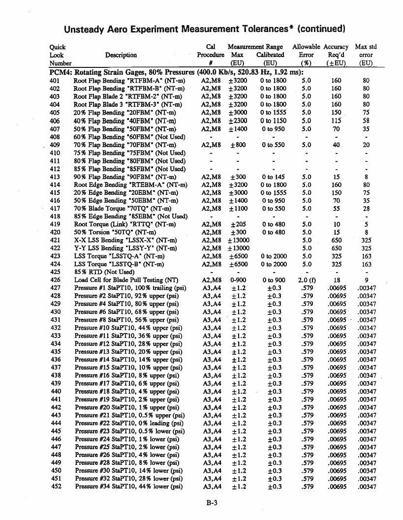
Unsteady Aero Experiment Measurement Tolerances* (continued)
Quick Cal Measurement Range Allowable Accuracy Max stdLook Description Procedure Max Calibrated Error Req'd errorNumber # (EU) (EU) (%) (±EU) (EU)
PCM4: Rotating Strain Gages, 80% Pressures (400.0 Kb/s, 520.83 Hz, 1.92 IDS):'401 Root Flap Bending WRTFBM-AW(NT-m) A2,MS ±3200 oto IS00 5.0 160 80402 Root Flap Bending wRTFBM-Bw (NT-m) A2,MS ±3200 O.to IS00 5.0 160 80403 Root Flap Blade 2 wRTFBM-2w(NT-m) A2,MS ±3200 oto IS00 5.0 160 SO404 Root Flap Blade 3 wRTFBM-3w(NT-m) A2,MS ±3200 oto.lS00 5.0 160 SO405 20 % Flap Bending w20FBMw(NT-m) A2,MS ±3000 oto 1555 5.0 150 . 75
406 40%Flap Bending -4OFBM- (NT-m) A2,M8 ±2300 oto 1150 5.0 115 58407 50% Flap Bending "SOFBM" (NT-m) A2,MS ±1400 oto 950 5.0 70 3540S 60% Flap Bending w60FBMw (Not Used)409 70% Flap Bending "70FBMw(NT-m) A2,MS ±SOO oto 550 5.0 40 20410 75 % Flap Bending "75FBMw (Not Used)411 SO% Flap Bending "SOFBMw(Not Used)412 S5% Flap Bending "85FBMw(Not Used)413 90% Flap Bending w90FBMw(NT-m) . A2,MS ±300 oto 145 5.0 15 S414 Root Edge Bending "RTEBM-A W(NT-m) A2,MS ±3200 oto 1800 5.0 160 80415 20 % Edge Bending w20EBMw(NT-m) A2,MS ±3000 oto 1555 5.0 150 75416 50% Edge Bending "50EBMw(NT-m) A2,MS ±1400 oto ·950 5.0 70 35417 70% Blade Torque "70TQ" (NT-m) A2,MS ±1100 oto 550 5.0 55 2S418 S5'% Edge Bending wS5EBM" (Not Used)419 Root Torque (Link) wRTTQw (NT-m) A2,MS ±205 oto 4S0 5.0 10 5420 50% Torsion w50TQ" (NT-m) A2,M8 ±300 oto 480 5.0 15 8421 X-X LSS Bending "LSSX-X" (NT-m) A2,MS ±13000 5.0 650 325422 y-y LSS Bending WLSSY-Y" (NT-m) A2,MS ±13000 5.0 650 325423 LSS Torque "LSSTQ-A" (NT-m) A2,MS ±6500 oto 2000 5.0 325 163424 LSS Torque "LSSTQ-B" (NT-m) A2,MS ±6500 oto 2000 5.0 325 163425 85 % RTD (Not Used)426 Load Cell for Blade Pull Testing (NT) A2,M8 0-900 oto 900 2.0 (f) 18 9427 Pressure #1 StaPTIO, 100% trailing (psi) A3,A4 ±1.2 ±0.3 .579 .00695 .00347428 Pressure #2 StaPTIO, 92% upper (psi) A3,A4 ±1.2 ±0.3 .579 .00695 .00347429 Pressure #4 StaPTIO, SO% upper (psi) A3,A4 ±1.2 ±0.3 .579 .00695 .00347430 Pressure #6 StaPTI0, 68 % upper (psi) A3,A4 ±1.2 ±0.3 .579 .00695 .00347431 Pressure #S StaPTI0, 56% upper (psi) A3,A4 ±1.2 ±0.3 .579 .00695 . .00347432 Pressure #10 StaPTI0, 44% upper (psi) A3,A4 ±1.2 ±0.3 .579 .00695 .00347433 Pressure #11 StaPTI0, 36% upper (psi) A3,A4 ±1.2 ±0.3 .579 .00695 .00347434 Pressure #12 StaPTIO, 2S % upper (psi) A3,A4 ±1.2 ±0.3 .579 .00695 .00347435 Pressure #13 StaPTI0, 20% upper (psi) A3,A4 ±1.2 ±0.3 .579 .00695 .00347
. 436 Pressure #14 StaPTI0, 14% upper (psi) A3,A4 ±1.2 ±O.3 .579 .00695 .00347437 Pressure #15 StaPTI0, 10% upper (psi) A3,A4 ±1.2 ±0.3 .579 .00695 .0034743S Pressure #16 StaPTI0, 8% upper (psi) A3,A4 ±1.2 ±0.3 .579 .00695 .00347439 Pressure #17 StaPTIO, 6% upper (psi) A3,A4 ±1.2 ±0.3 .579 .00695 .00347440 Pressure #IS StaPTI0, 4% upper (psi) A3,A4 ±1.2 ±O.3 .579 .00695 .00347441 Pressure #19 StaPTI0, 2 % upper (psi) A3,A4 ±1.2 ±0.3 .579 .00695 .00347442 Pressure #20 StaPTI0, 1.% upper (psi) A3,A4 ±1.2 ±0.3 ·.579 .00695 .00347443 Pressure #21 StaPTI0, 0.5 % upper (psi) A3,A4 ±1.2 ±0.3 .579 .00695 .00347444 Pressure #22 StaPTI0, 0% leading (psi) A3,A4 ±1.2 ±0.3 .579 .00695 .00347445 Pressure m StaPTI0, 0.5 % lower (psi) A3,A4 ±1.2 ±0.3 .579 .00695 .00347446 Pressure #24 StaPTI0, 1% lower (psi) A3,A4 ±1.2 ±0.3 .579 .00695 .00347447 Pressure #25 StaPTI0, 2% lower (psi) A3,A4 ±1.2 ±O.3 .579 .00695 .00347448 Pressure #26 StaPTI0, 4% lower (psi) A3,A4 ±1.2 ±0.3 .579 .00695 .00347449 Pressure #28 StaPTI0, S% lower (psi) A3,A4 ±1.2 ±0.3 .579 .00695 .00347450 Pressure #30 StaPTI0, 14% lower (psi) A3,A4 ±1.2 ±O.3 .579 .00695 .00347451 Pressure #32 StaPTI0, 2S% lower (psi) A3,A4 ±1.2 ±0.3 .579 .00695 .00347452 Pressure #34 StaPTI0, 44% lower (psi) A3,A4 ±1.2 ±O.3 .579 .00695 .00347
B-3

Unsteady Aero Experiment Measurement Tolerances" (continued)
Quick Cal Measurement Range Allowable Accuracy Max stdLook Description Procedure Max Calibrated Error Req'd errorNumber # (BU) (BU) (%) (±EU) (BU)PCM4: Continued (400.0 Kb/s, 520.83 Hz, 1.92 ms)453 Pressure #36 StaPT10, 68 % lower (psi) A3,A4 ±1.2 ±0.3 .579 .00695 .00347454 Pressure #38 StaPT10, 92 % lower (psi) A3,A4 ±1.2 ±0.3 .579 .00695 .00347455 Pressure #1~ StaPT9, 4% upper (psi) A3,A4 ±1.2 ±0.3 .500 .00600 .00300456 Pressure #11 StaPT9, 36% upper (psi) A3,A4 ±1.2 ±0.3 .500 .00600 .00300457 Pressure #11 StaPT8,36% upper (psi) A3,A4 ±1.2 ±0.3 .439 .00527 .00264458 Total Pressure Probe, 86 % span (psi) A3,A4 ±1.2 ±0.3 .579 .00695 .00347459 Absolute Reference Pressure (mb) E3 800-1100 711-914 2.0 3.0 1.5460 Calibration Pressure (psi) (Cal Only) E2 ±0.3 ±0.5 .222 (f) .00133 .00044**461 Pitch Angle (degrees) M3 -106 to 71 -10 to 20 1.0 1.0 .5462 PCM Voltage Monitor (Quick-Look Only) ±140 10 14 7
PCM8: Rotating 30% and 40% Pressures (400.0 Kb/s, 520.83 Hz, 1.92 ms):801 Absolute Reference Pressure (Not Used)802 Calibration Pressure (Cal Only) E2 ±0.3 ±0.5 .222 (f) .00133 .00044**803 Spare804 Pressure #1 StaPT1, 100% trailing (psi) A2,A3 ±0.43 ±0.3 .310 .00133 .00067805 Pressure #4 StaPT1, 80% upper (psi) A2,A3 ±0.43 ±0.3 .310 .00133 .00067806 Pressure #6 StaPT1, 68% upper (Psi) A2,A3 ±0.43 ±0.3 .310 .00133 .00067807 Pressure #8 StaPT1, 56 % upper (Psi) A2,A3 ±0.43 ±0.3 .310 .00133 .00067808 Pressure #10 StaPT1, 44% upper (psi) A2,A3 ±0.43 ·± 0.3 .310 .00133 .00067809 Pressure #11 StaPT1, 36% upper (psi) A2,A3 ±0.43 ±0.3 .310 .00133 .00067810 Pressure #13 StaPT1, 20% upper (psi) A2,A3 ±0.43 ±0.3 .310 .00133 .00067811 Pressure #14 StaPT1, 14% upper (psi) A2,A3 ±0.43 ±0.3 .310 .00133 .00067812 Pressure #15 StaPT1, 10% upper (psi) A2,A3 ±0.43 ±0.3 .310 .00133 .00067813 Pressure #16 StaPT1, 8% upper (psi) A2,A3 ±0.43 ±0.3 .310 .00133 .00067814 Pressure #17 StaPT1, 6% upper (psi) A2,A3 ±0.43 ±0.3 .310 .00133 .00067815 Pressure #18 StaPTl, 4% upper (psi) A2,A3 ±0.43 ±0.3 .310 .00133 .00067816 Pressure #19 StaPT1, 2% upper (psi) A2,A3 ±0.43 ±0.3 .310 .00133 .00067817 Pressure #21 StaPTl, 0.5% upper (psi) A2,A3 ±0.43 ±0.3 .310 .00133 .00067818 Pressure #22 StaPTl, 0% leading (psi) A2,A3 ±0.43 ±0.3 .310 .00133 .00067819 Pressure #23 StaPT1, 0.5% lower (psi) A2,A3 ±0.43 ±0.3 .310 .00133 .00067820 Pressure #24 StaPT1, 1% lower (psi) A2,A3 ±0.43 ±0.3 .310 .00133 .00067821 Pressure #2S StaPT1, 2 % lower (psi) A2,A3 ±0.43 ±0.3 .310 .00133 .00067822 Pressure #26 StaPT1, 4% lower (psi) A2,A3 ±0.43 ±0.3 .310 .00133 .00067823 Pressure #28 StaPTl, 8% lower (psi) A2,A3 ±0.43 ±0.3 .310 .00133 .00067824 Pressure #30 StaPT1, 14% lower (psi) A2,A3 ±0.43 ±0.3 .310 .00133 .00067825 Pressure #31 StaPTl, 20% lower (psi) A2,A3 ±0.43 ±0.3 .•310 .00133 .00067826 Pressure #34 StaPT1, 44% lower (psi) A2,A3 ±0.43 ±0.3 .310 .00133 .00067827 Pressure #36 StaPT1, 68 % lower (Psi) A2,A3 ±0.43 ±0.3 .310 .00133 .00067828 Pressure #38 StaPT1, 92%' lower (psi) A2,A3 ±0.43 ±0.3 .310 .00133 .00067829 Pressure #18 StaPT2, 4% upper (psi) A2,A3 ±0.43 ±0.3 .404 .00174 .00087830 Pressure #11 StaPT2, 36 % upper (psi) A2,A3 ±0.43 ±0.3 .404 .00174 .00087831 Pressure #11 StaPT3, 36% upper (psi) A2',A3 ±0.43 ±0.3 .495 .00213 .00106832 Total Pressure Probe, 34 % span (psi) A2,A3 ±0.43 ±0.3 .310 .00133 .00067833 Pressure #1 StaPT4, 100% trailing (psi) A2,A3 ±0.43 ±0.3 .620 .00267 .00133834 Pressure #2 StaPT4, 92% upper (psi) A2,A3 ±0.43 ±0.3 .620 - .00267 .00133835 Pressure #4 StaPT4, 80% upper (psi) A2,A3 ±0.43 ±0.3 .620 .00267 .00133836 Pressure #6 StaPT4, 68% upper (psi) A2,A3 ±0.43 ±0.3 .620 .00267 .00133837 Pressure #8 StaPT4, 56 % upper (psi) A2,A3 ±0.43 ±0.3 .620 .00267 .00133838 Pressure #10 StaPT4, 44% upper (psi) A2,A3 ±0.43 ±0.3 .620 .00267 .00133839 Pressure #11 StaPT4, 36 % upper (psi) A2,A3 ±0.43 ±0.3 .620 .00267 .00133840 Pressure #12 StaPT4, 28 % upper (psi) A2,A3 ±0.43 ±0.3 .620 .00267 .00133
B-4

Unsteady Aero Experiment Measurement Tolerances* (continued)
Quick Cal Measurement Range Allowable Accuracy Max stdLook Description Procedure Max Calibrated Error Req'd " errorNumber # (EU) (ED) (%) (±EU) (EU)PCM8: Continued (400.0 Kb/s, 520.83 Hz, 1.92 ms):841 Pressure #13 StaPT4, 20% upper (psi) A2,AJ ±0.43 ±0.3 .620 .00267 .00133842 Pressure #14 StaPT4, 14% upper (Psi) A2,AJ ±0.43 ±0.3 .620 .00267 .00133843 Pressure #15 StaPT4, 10% upper (psi) A2,AJ ±0.43 ±0.3 .620 .00267 .00133844 Pressure #16 StaPT4, 8 % upper (psi) A2,AJ ±0.43 ±0.3 .620 .00267 .00133845 Pressure #17 StaPT4, 6 % upper (psi) A2,AJ ±0.43 ±0.3 .620 .00267 .00133846 Pressure #18 StaPT4, 4% upper (psi) A2,AJ ±0.43 . ±0.3 .620 .00267 .00133847 P~ #19 StaPT4, 2 % upper (psi) A2,AJ ±0.43 ±0.3 .620 .00267 .00133848 Pressure #20 StaPT4, 1% upper (Psi) A2,AJ ±0.43 ±0.3 .620 .00267 .00133849 Pressure #21 StaPT4, 0.5 % upper (psi) ~,AJ ±0.43 ±0.3 .620 .00267 .00133850 Pressure #22 StaPT4, 0% leading (psi) A2,AJ ±0.43 ±0.3 .620 .00267 .00133851 Pressure #23 StaPT4, 0.5 % lower'(psi) A2,AJ ±0.43 ±0.3 .620 .00267 .00133852 Pressure #2S StaPT4, 2% lower (psi) A2,AJ ±0.43 ±0.3 .620 .00267 .00133853 Pressure #26 StaPT4, 4% lower (psi) A2,AJ ±0.43 ±0.3 .620 .00267 .00133854 Pressure #27 StaPT4, 6% lower (psi) A2,AJ ±0.43 ±0.3 .620 .00267 .00133855 Pressure #28 StaPT4, 8% lower (psi) - A2,AJ ±0.43 ±0.3 .620 .00267 .00133856 Pressure #30 StaPT4, 14% lower (psi) A2,AJ ±0.43 ±0.3 .620 .00267 .00133857 Pressure #32 StaPT4, 28% lower (psi) A2,AJ ±0.43 ±0.3 .620 .00267 .00133858 Pressure #34 StaPT4, 44 % lower (psi) A2,A3 ±0.43 ±0.3 .620 .00267 .00133859 Pressure #36 StaPT4, 68 % lower (psi) A2,AJ ±0.43 ±0.3 .620 .00267 .00133860 Pressure #38 StaPT4, 92 % lower (psi) A2,AJ ±0.43 ±0.3 .620 .00267 .00133861 Pressure #18 StaPT3, 4% upper (psi) A2,AJ ±0.43 ±0.3 .495 .00213 .00106862 Total Pressure Probe, 50.6 % span (psi) A2,AJ ±0.43 ±0.3 .620 .00267 .00133
PCM9: Rotating 63% Pressures, Angle of Attack (400.0 Kb/s, 520.83 Hz, 1.92 ms):901 Pressure #11 StaPTS, 36 % upper (psi) A2,AJ ±1.2 ±0.3 .262 .00317 .00159902 Pressure #18 StaPT5, 4% upper (psi) A2,AJ ±1.2 ±0.3 .262 .00317 .00159903 Pressure #1 StaPT7, 100% trailing (psi) A2,AJ ±1.2 ±0.3 .372 .00447 .00223904 Pressure #2 StaPT7, 92 % upper (psi) A2,AJ ±1.2 ±0.3 .372 .00447 .00223905 Pressure #4 StaPT7, 80 % upper (psi) A2,AJ ±1.2 ±0.3 .372 .00447 .00223906 Pressure #6 StaPT7, 68 % upper (psi) A2,A3 ±1.2 ±0.3 .372 .00447 .00223907 Pressure #8 StaPT7, 56 % upper (psi) A2,AJ ±1.2 ±0.3 .372 .00447 .00223908 Pressure #10 StaPT7, 44% upper (psi) A2,AJ ±1.2 ±0.3 .372 .00447 .00223909 Pressure #11 StaPT7, 36 % upper (psi) A2,A3 ±1.2 ±0.3 .372 .00447 .00223910 Pressure #12 StaPT7, 28 % upper (psi) A2,AJ ±1.2 ±0.3 .372 .00447 .00223911 Pressure #13 StaPT7, 20 % upper (psi) A2,AJ ±1.2 ±0.3 .372 .00447 .00223912 Pressure #14 StaPT7, 14% upper (psi) A2,AJ ±1.2 ±0.3 .372 .00447 .00223913 Pressure #15 StaPT7, 10 % upper (psi) A2,A3 ±1.2 ±0.3 .372 .00447 .00223914 Pressure #16 StaPT7, 8 % upper (psi) A2,AJ ±1.2 ±0.3 .372 .00447 .00223915 Pressure #17 StaPT7, 6% upper (psi) A2,AJ ±1.2 ±0.3 .372 .00447 .00223916 Pressure #18 StaPT7, 4% upper (psi) A2,A3 ±1.2 ±0.3 .372 .00447 .00223917 Pressure #19 StaPT7, 2 % upper (psi) A2,AJ ±1.2 ±0.3 .372 .00447 .00223918 Pressure #20 StaPT7, 1% upper (psi) A2,AJ ±1.2 ±0.3 .372 .00447 .00223919 Pressure #21 StaPT7, 0.5 % upper (psi) A2,AJ ±1.2 ±0.3 .372 .00447 .00223920 Pressure #22 StaPT7, 0% leading (psi) A2,AJ ±1.2 ±0.3 .372 .00447 .00223921 Pressure #23 StaPT7, 0.5% lower (psi) A2,AJ ±1.2 ±0.3 .372 .00447 .00223922 Pressure #24 StaPT7, 1 % lower (psi) A2,AJ ±1.2 ±0.3 .372 .00447 .00223923 Pressure #2S StaPT7, 2 % lower (psi) A2,AJ ±1.2 ±0.3 .372 .00447 .00223924 Pressure #26 StaPT7, 4 % lower (psi) A2,A3 ±1.2 ±0.3 .372 .00447 .00223925 Pressure #28 StaPT7, 8 % lower (psi) A2,AJ ±1.2 ±0.3 .372 .00447 .00223926 Pressure #30 StaPT7, 14% lower (psi) A2,AJ ±1.2 ±O.3 .372 .00447 .00223927 Pressure #32 StaPT7, 28 % lower (psi) A2,AJ ±1.2 ±0.3 .372 .00447 .00223 .928 Pressure #34 StaPT7, 44 % lower (psi) A2,AJ ±1.2 ±0.3 .372 .00447 .00223
B-5

Unsteady Aero Experiment Measurement Tolerances* (continued)
Quick Cal Measurement Range Allowable Accuracy Max stdLook Description Procedure Max Calibrated Error Req'd errorNumber # (EU) (EU) (%) (±EU) (EU)PCM9: Continued (400.0 Kb/s, 520.83 Hz, 1.92 ms):929 Pressure #36 StaPTI, 6~% lower (Psi) A2,A3 ±1.2 ±0.3 .372 .00447 .00223930 Pressure #38 StaPTI; 92% lower (psi) A2,A3 ±1.2 ±0.3 .372 .00447 .00223931 Pressure #18 StaPT6, 4% upper (psi) . A2,A3 ±1.2 ±0.3 .321 .00386 .00192932 Pressure #18 StaPT8, 4% upper (psi) A2,A3 ±1.2 :to.3 .439 .00527 .00264933 Pressure #11 StaPT6, 36 % upper (Psi) A2,A3 ±1.2 ±0.3 .321 .00386 .00192934 Total Pressure Probe, 67.3 % span (psi) A2,A3 ±1.2 ±0.3 .372 .00447 .00223935 Angle-of-Attack, 86% span (degrees) M2 -22 to 55 -20 to 40 2.6 1.0 .5936 Ground937 Angle-of-Attack, 67.3 % span (degrees) M2 -22 to 55 -20 to 40 2.6 1.0 .5938 Ground939 Do Not Use (Bad channel)940 Ground941 Angle-of-Attack, 34% span (degrees) M2 -22 to 55 -20 to 40 2.6 1.0 .5942 Ground943 Nitrogen Pressure (psi) (Quick-Look Only) ±2000 10 200 100944 +15 Volt Power Monitor (V) (Quick-Look Only)- ±20 10 1.5 .8945 -15 Volt Power Monitor (V) (Quick-Look Only) - ±20 10 1.5 .8946 Angle-of-Attack, 50.6 % span (degrees) M2 -22 to 55 -20 to 40 2.6 1.0 .5947 DC Ground Monitor (counts) (Quick-Look Only) - oto 4095948 Spare949 Spare950 Spare951 Spare952 Spare953 Absolute Reference Pressure E3 800-1100 711-914 2.0 3.0 1.5954 Calibration Pressure (Cal Only) E4 ±0.3 ±0.5 .222 (f) .00133 .00044**955 Spare956 Spare957 Spare958 Spare959 Spare960 Spare961 Spare962 Spare
Notes
* All measured channels and their corresponding calibration requirements are listed here. The first columnshows channel ID number as it is referenced by the Quick-Look system. The first digit is the PCM streamnumber and the next two digits are the PCM frame number. Column 2 contains channel descriptions and units.Each channel has defined calibration procedures identified in column 3 which are performed to measure the end toend accuracy of all channels. The procedures are identified by the letter A, E or M, followed by a number. Theletter designates 3 basic types of calibrations An WEWdesignates those channels in which the transducer requiresan external calibration, such as anamometers in the wind tunnel. An WAWdesignates an automatic calibration inwhich many incoming signals can be automatically placed in a known calibration state. An wM w designatescalibrations which require manual placement of transducers into a position to enable calibrating. The numberwhich follows identifies a specific procedure to be followed in order to calibrate that channel. These aredescribed in detail in Appendix D. Channels with type wEw calibrations are done in two parts in which thetransducer and electronics are calibrated separately, then RMS summed to determine overall channel accuracy.All other channels are end-to-end calibrated to directly measure the full channel response. Some channels (such aspressures and strain-gages) require two end-to-end cals, one to calculate slope, and another to calculate offset.
B-6
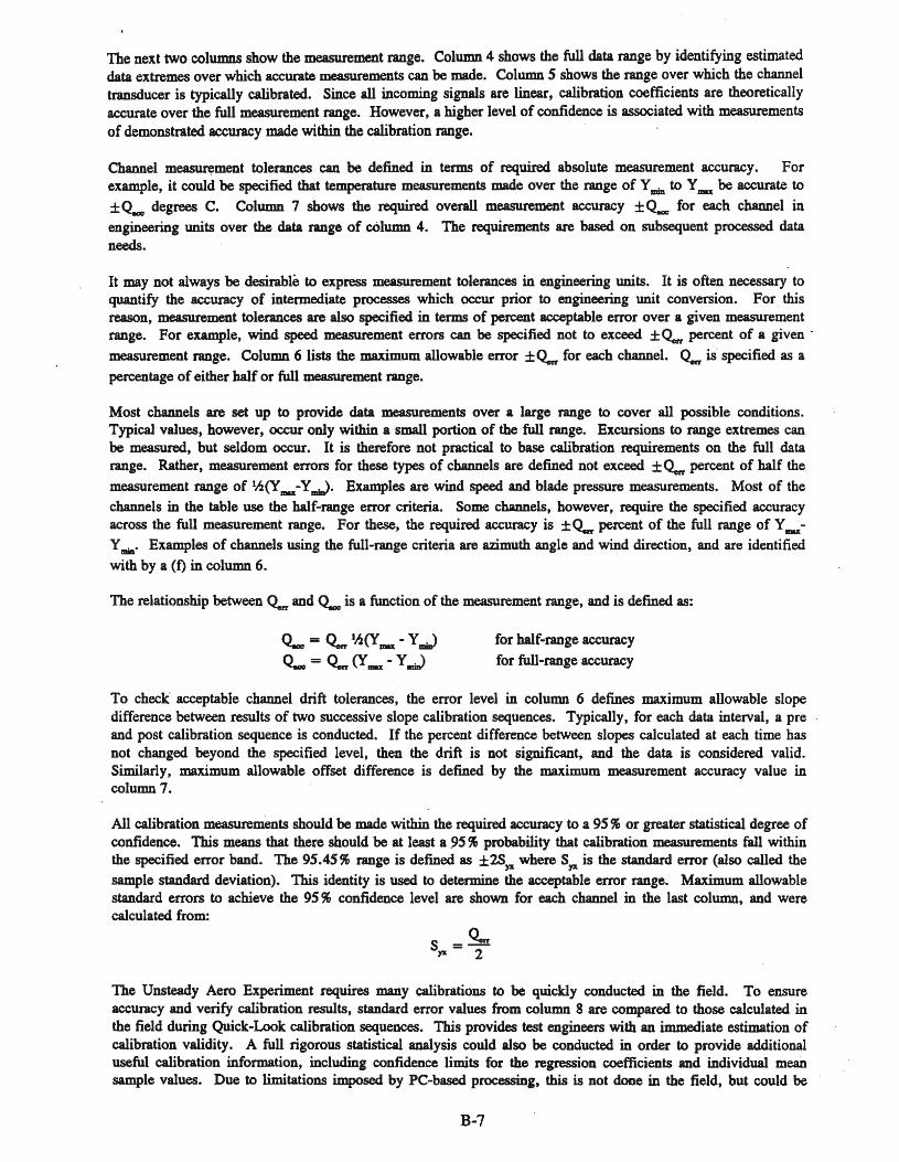
The next two columns show the measurement range. Column 4 shows the full data range by identifying estimateddata extremes over which accurate measurements can be made. Column 5 shows the range over which the channeltransducer is typically calibrated. Since all incoming signals are linear, calibration coefficients are theoreticallyaccurate over the full measurement range. However, a higher level of confidence is associated with measurementsof demonstrated accuracy made within the calibration range.
Channel measurement tolerances can be defined in terms of required absolute measurement accuracy. Forexample, it could be specified that temperature measurements made over the range of Ymin to Y_ be accurate to
±~ degrees C. Column 7 shows the required overall measurement accuracy ±~ for each channel in
engineering units over the data range of column 4. The requirements are based on subsequent processed dataneeds.
It may not always be desirable to express measurement tolerances in engineering units. It is often necessary toquantify the accuracy of intermediate processes which occur prior to engineering unit conversion. For thisreason, measurement tolerances are also specified in terms of percent acceptable error over a given measurementrange. For example, wind speed measurement errors can be specified not to exceed ±o.r percent of a given '
measurement range. Column 6 lists the maximum allowable error ±Q., for each channel. Q., is' specified as a
percentage of either half or full measurement range.
Most channels are set up to provide data measurements over a large range to cover all possible conditions.Typical values, however, occur only within a small portion of the full range. Excursions to range extremes canbe measured, but seldom occur. It is therefore not practical to base calibration requirements on the full datarange. Rather, measurement errors for these types of channels are defined not exceed ±<4n percent of half the
measurement range of 11.z(Y_-Ymm>. Examples are wind speed and blade pressure measurements. Most of the
channels in the table use the half-range error criteria. Some channels, however, require the specified accuracyacross the full measurement range. For these, the required accuracy is ±o.r percent of the full range of Y~
Ymin. Examples of channels using the full-range criteria are azimuth angle and wind direction, and are identified
with by a (f) in column 6.
The relationship between <4n and~ is a function of the measurement range, and is defined as:
~ = Q., Ih(Y_ - Y.,)~ = <4n (Y_ - YrmJ
for half-range accuracy
for full-range accuracy
To check acceptable channel drift tolerances, the error level in column 6 defines maximum allowable slopedifference between results of two successive slope calibration sequences. Typically, for each data interval, a preand post calibration sequence is conducted. If the percent difference between slopes calculated at each time hasnot changed beyond the specified level, then the drift is not significant, and the data is considered valid.Similarly, maximum allowable offset difference is defined by the maximum measurement accuracy value incolumn 7.
All calibration measurements should be made within the required accuracy to a 95% or greater statistical degree ofconfidence. This means that there should be at least a .95% probability that calibration measurements fall withinthe specified error band. The 95.45% range is defined as ±2Sya where Sya is the standard error (also called the
sample standard deviation). This identity is used to determine the acceptable error range. Maximum allowablestandard errors to achieve the 95% confidence level are shown for each channel in the last column, and werecalculated from:
s = o..mya 2
The Unsteady Aero Experiment requires many calibrations to be quickly conducted in the field. To ensureaccuracy and verify calibration results, standard error values from column 8 are compared to those calculated inthe field during Quick-Look calibration sequences. This provides test engineers with an immediate estimation ofcalibration validity. A full rigorous statistical analysis could also be conducted in order to provide additionaluseful calibration information, including confidence limits for the regression coefficients and individual meansample values. Due to limitations imposed by PC-based processing, this is not done in the field, but could be
B-7

post-calculated if required. 95 % confidence limits for least-squares regression slope value m are determinedfrom:
t.m S_m±--~..JiM. S..
where t.lnS is the student t distribution for N samples at the .975 level (use 5% significance I 2), and S.. is the
standard deviation of the measured X values. Similarly, 95 % confidence limits for the mean sample values can bedetermined using standard statistical techniques:
I ~ oc,-X>,Yo ± _~ S1" 1+ S 2
-vN-2 ..
where X is the mean of the measured X values and Yo is the predicted value of Y at X = Xo using the resulting
calculated regression slope m and offset b, ie, Yo = mXo + b.
•• For calibrating pressures, the refrence transducer is calibrated to a 99 % confidence level that measurementscan be made to a required accuracy of ± ,(>0133 psi accros the full calibration range of ± .3 psi. The 99.73 %level is defined as ± 3S1'" which is typically used when calibrating reference transducers from which other
calibrations are derived. For pressure calibrations, required pressure measurement accuracy is 10% of the totalinduced pressure.
B-8

Appendix C
Unsteady Aero Experiment Channel Data Rates
C-l

Unsteady Aero Experiment Channel Data Rates
QuicklEXP Filter DeclBW Sample No. PerLookrrag Description Setting (NthSeql) Rate DT 144 msecNumber (Hz) (Hz) (Hz) (msec) recordPCM1: North Met Tower (7.5 Kb/s, 34.72 Hz, 28.8 ms):10111301 20 M Hot Film (Not Used) 5/1 6.94 144.0 1102/1302 18 M Sonic Channel A (Not Used) 5/1 6.94 144.0 1103/1303 18 M Sonic Channel B (Not Used) 5/1 6.94 144.0 1104/1304 18 M Sonic Channel C (Not Used) 5/1 6.94 144.0 1105/1305 5 M Wind Direction (Not Used) 1 5/1 6.94 144.0 1106/1306 5 M Wind Speed 1 5/1 6.94 144.0 1107/1307 10 M Wind Direction (Not Used) 1 5/1 6.94 144.0 1108/1308 10 M Wind Speed 1 5/1 6.94 144.0 1109/1309 20 M Wind Direction (Not Used) 1 5/1 6.94 144.0 1110/1310 20 M Wind Speed 1 5/1 6.94 144.0 1111/1311 50 M Wind Direction (Not Used) 1 5/1 6.94 144.0 1112/1312 50 M Wind Speed 1 5/1 6.94 144.0 1113/1313 5 M Air Temperature 1 5/1 6.94 144.0 1114/1314 Delta Temperature 1 5/1 6.94 144.0 1115/1315 5 M DP (Not Used) 5/1 6.94 144.0 1116/1316 Baro Pressure 1 5/1 6.94 144.0 1
PCM2: Vertical Plane Array (15.0 Kb/s, 69.44 Hz, 14.4 ms):20110201 VPA Prop Vane WS-l 2 5/2 13.9 72.0 2202/0202 VPA Prop Vane WS-2 2 5/2 . 13.9 72.0 2203/0203 VPA Prop Vane WS-3 2 5/2 13.9 72.0 2204/0204 VPA Prop Vane WS-4 2 5/2 13.9 72.0 2205/0205 VPA Prop Vane WS-5 2 5/2 13.9 72.0 2206/0206 VPA Prop Vane WS-6 2 5/2 13.9 72.0 2207/0207 VPA Prop Vane WS-7 2 5/2 13.9 72.0 2208/0208 VPA Prop Vane WS-8 2 5/2 13.9 72.0 2209/0209 VPA PV Hub Height WS-9 2 5/2 13.9 72.0 2210/0210 VPA PV Hub Height WD-9 2 5/2 13.9 72.0 221110211 VPA Bi-Vane WS-12 2 5/2 13.9 72.0 2212/0212 VPA Bi-Vane WD-12 2 5/2 13.9 72.0 2213/0213 VPA Bi-Vane Wa-12 2 5/2 13.9 72.0 2214/0214 VPA Bi-Vane WS-13 2 5/2 13.9 72.0 2215/0215 VPA Bi-Vane WD-13 2 5/2 13.9 72.0 2216/0216 VPA Bi-Vane Wa-13 2 5/2 13.9 72.0 2
PCM3: VPA, Local Met, Tower, Turbine (60.0 Kb/s, 277.78 Hz, 3.6 ms):30110301 VPA Prop Vane WS-lO 2 20/2 13.9 72.0 2302/0302 VPA Prop Vane WS-11 2 20/2 13.9 72.0 2303/0303 LSS Azimuth Angle 32 0/54 277.78 3.6 40304/0304 Yaw Moment 40 0/54 277.78 3.6 40305/0305 Tower Bending E-W 40 0/54 277.78 3.6 40306/0306 Tower Bending N-S 40 0/54 277.78 3.6 40307/0307 Yaw Angle 10 5/11 55.56 18.8 8308/0308 Generator Power 54 0/54 277.78 3.6 40309/0309 LSS Speed (Not Used) 40/1 6.94 144.0 1310/0310 TSI (South) X-Film U (Not Used) 40/1 6.94 144.0 1311/0311 TSI (South) X-Film W (Not Used) 40/1 6.94 144.0 1312/0312 TSI (North) X-Film U (Not Used) 40/1 6.94 144.0 1313/0313 TSI (North) X-Film W (Not Used) 40/1 6.94 144.0 1314/0314 Sonic Anemometer Ch A (Not Used) 40/1 6.94 144.0 1315/0315 Sonic Anemometer Ch B (Not Used) 40/1 6.94 144.0 1316/0316 Sonic Anemometer Ch C (Not Used) 40/1 6.94 144.0 1
C-2
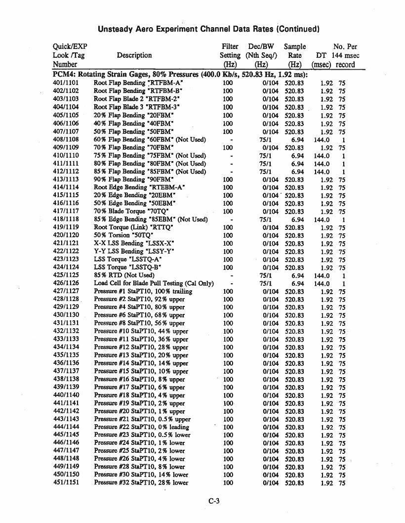
Unsteady Aero Experiment Channel Data Rates (Continued)
QuicklEXP Filter DecfBW Sample No. PerLook !fag Description Setting (Nth Seq/) Rate DT 144 msecNumber (Hz) (Hz) (Hz) (msec) recordPCM4: Rotating Strain Gages, 80% Pressures (400.0 Kb/s, 520.83 Hz, 1.92 ms):40111101 Root Flap Bending ~RTFBM-A" 100 0/104 520.83 1.92 7540211102 Root Flap Bending "RTFBM-B" 100 0/104 520.83 1.92 75403/1103 Root Flap Blade 2 "RTFBM-2· 100 01104 520.83 1.92 75404/1104 Root Flap Blade 3 "RTFBM-3" 100 0/104 520.83 1.92 7540511105 20 % Flap Bending "20FBM" 100 0/104 520.83 1.92 7540611106 40% Flap Bending "4OFBM" 100 0/104 520.83 1.92 7540711107 50% Flap Bending "50FBM" 100 0/104 520.83 1.92 75408/1108 60% Flap Bending "60FBM" (Not Used) 75/1 6.94 144.0 1409/1109 70% Flap Bending "70FBM" 100 0/104 520.83 1.92 75410/1110 75 % Flap Bending "75FBM" (Not Used) 75/1 6.94 144.0 1411/1111 80% Flap Bending "80FBM" (Not Used) 75/1 6.94 144.0 1412/1112 85 % Flap Bending "8SFBM" (Not Used) 75/1 6.94 144.0 141311113 90% Flap Bending "90FBM" 100 01104 520.83 1.92 75414/1114 Root Edge Bending "RTEBM-A" 100 0/104 520.83 1.92 75415/1115 20 % Edge Bending "20EBM" 100 0/104' 520.83 1.92 75416/1116 50% Edge Bending "SOEBM" 100 0/104 520.83 1.92 7541711117 70% Blade Torque "70TQ" 100 0/104 520.83 1.92 75418/1118 85% Edge Bending "8SEBM" (Not Used) 75/1 6.94 144.0 141911119 Root Torque (Link) "RTTQ" 100 0/104 520.83 1.92 7542011120 50% Torsion "SOTQ" 100 0/104 520.83 1.92 7542111121 X-X LSS Bending "LSSX-X" 100 01104 520.83 1.92 7542211122 Y-Y LSS Bending "LSSY-Y" 100 0/104 520.83 1.92 7542311123 LSS Torque "LSSTQ-A" 100 0/104 520.83 1.92 75424/1124 LSS Torque "LSSTQ-B" 100 0/104 520.83 1.92 75425/1125 85% RTD (Not Used) 75/1 6.94 144.0 1426/1126 Load Cell for Blade Pull Testing (Cal Only) 7511 6.94 144.0 142711127 Pressure #1 StaPTI0, 100% trailing 100 0/104 520.83 1.92 7542811128 Pressure #2 StaPTI0, 92% upper 100 0/104 520.83 1.92 75429/1129 Pressure #4 StaPTI0, 80% upper 100 0/104 520.83 1.92 75430/1130 Pressure #6 StaPTI0, 68 % upper 100 0/104 520.83 1.92 75431/1131 Pressure #8 StaPTI0, 56% upper 100 01104 520.83 1.92 75432/1132 Pressure #10 StaPT10, 44% upper 100 0/104 520.83 1.92 75 ·433/1133 Pressure #11 StaPTI0, 36% upper 100 0/104 520.83 1.92 75434/1134 Pressure #12 StaPTI0, 28 % upper 100 0/104 520.83 1.92 75435/1135 Pressure #13 StaPTI0, 20% upper 100 0/104 520.83 1.92 75436/1136 Pressure #14 StaPTI0, 14% upper 100 0/104 520.83 1.92 75437/1137 Pressure #15 S~10, 10% upper 100 0/104 520.83 1.92 75438/1138 Pressure #16 StaPTI0, 8% upper 100 0/104 520.83 1.92 7543911139 Pressure #17 StaPTI0, 6% upper 100 0/104 520.83 1.92 75440/1140 Pressure #18 StaPTI0, 4% upper 100 0/104 520.83 1.92 75441/1141 Pressure #19 StaPTI0, 2 % upper 100 01104 520.83 1.92 75442/1142 Pressure #20 StaPTI0, 1% upper 100 0/104 520.83 1.92 75443/1143 Pressure #21 StaPTI0, 0.5 % upper 100 0/104 520.83 1.92 75444/1144 Pressure #22 StaPTI0, 0% leading 100 0/104 520.83 1.92 75445/1145 Pressure #23 StaPTI0, 0.5% lower 100 0/104 520.83 1.92 75446/1146 Pressure #24 StaPTI0, 1% lower 100 0/104 520.83 1.92 75447/1147 Pressure #2S StaPTI0, 2 % lower 100 0/104 520.83 1.92 75448/1148 Pressure #26 StaPTI0, 4% lower 100 0/104 520.83 ·1.92 75449/1149 Pressure #28 StaPTI0, 8% lower 100 0/104 520.83 1.92 75450/1150 Pressure #30 StaPTI0, 14% lower 100 0/104 520.83 1.92 7545111151 Pressure #32 StaPTI0, 28% lower 100 0/104 520.83 1.92 75
C-3
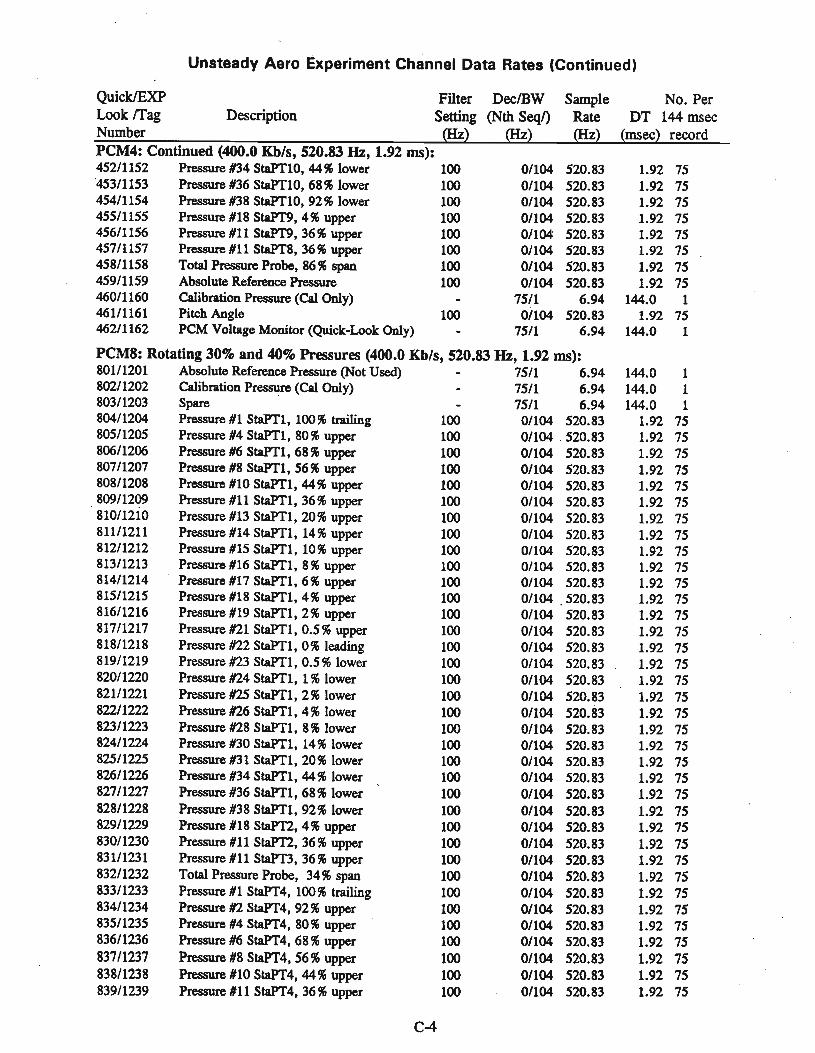
Unsteady Aero Experiment Channel Data Rates (Continued)
QuicklEXP Filter DeclBW Sample No. PerLook fI'ag Description Setting (NthSeql) Rate DT 144 msecNumber (Hz) (Hz) (Hz) (msec) recordPCM4: Continued (400.0 Kb/s, 520.83 Hz, 1.92 ms):452/1152 Pressure #34 StaPf10, 44 % lower 100 0/104 520.83 1.92 75"453/1153 Pressure #36 StaPf10, 68 % lower 100 0/104 520.83 1.92 75454/1154 Pressure #38 StaPf10, 92 % lower 100 0/104 520.83 1.92 75455/1155 Pressure #18 Sta.PT9, 4% upper 100 0/104 520.83 1.92 75456/1156 Pressure #11 Sta.PT9, 36% upper 100 0/104 520.83 1.92 75457/1157 Pressure #11 StaPf8, 36 % upper 100 0/104 520.83 1.92 75458/1158 Total Pressure Probe, 86 % span 100 0/104 520.83 1.92 75459/1159 Absolute Reference Pressure 100 0/104 520.83 1.92 75460/1160 Calibration Pressure (Cal Only) 75/1 6.94 144.0 1461/1161 Pitch Angle 100 0/104 520.83 1.92 75462/1162 PCM Voltage Monitor (Quick-Look Only) 75/1 6.94 144.0 1
PCM8: Rotating 30% and 40% Pressures (400.0 Kb/s, 520.83 Hz, 1.92 ms):801/1201 Absolute Reference Pressure (Not Used) 75/1 6.94 144.0 1802/1202 Calibration Pressure (Cal Only) 75/1 6.94 144.0 1803/1203 Spare 75/1 6.94 144.0 1804/1204 Pressure #1 StaPf1, 100% trailing 100 01104 520.83 1.92 75805/1205 Pressure #4 StaPf1, 80% upper 100 0/104 . 520.83 1.92 75806/1206 Pressure #6 StaPf1, 68% upper 100 0/104 520.83 1.92 75807/1207 Pressure #8 StaPf1, 56 % upper 100 0/104 520.83 1.92 75808/1208 Pressure #10 StaPf1, 44% upper 100 01104 520.83 1.92 75809/1209 Pressure #11 StaPT1, 36% upper 100 0/104 520.83 1.92 75810/1210 Pressure #13 StaPT1, 20% upper 100 0/104 520.83 1.92 75811/1211 Pressure #14 StaPf1, 14% upper 100 0/104 520.83 1.92 75812/1212 Pressure #15 StaPT1, 10% upper 100 01104 520.83 1.92 75813/1213 Pressure #16 StaPf1, 8 % upper 100 01104 520.83 1.92 75814/1214 Pressure #17 StaPf1, 6% upper 100 0/104 520.83 1.92 75815/1215 Pressure #18 StaPT1, 4% upper 100 0/104 520.83 1.92 75816/1216 Pressure #19 StaPf1, 2% upper 100 0/104 520.83 1.92 75817/1217 Pressure #21 StaPf1, 0.5% upper 100 0/104 520.83 1.92 75818/1218 Pressure #22 StaPf1, 0% leading 100 01104 520.83 1.92 75819/1219 Pressure #23 StaPf1, 0.5% lower 100 0/104 520.83 1.92 75820/1220 Pressure #24 StaPT1, 1% lower 100 0/104 520.83 1.92 75821/1221 Pressure #2S StaPf1, 2% lower 100 0/104 520.83 1.92 75822/1222 Pressure #26 StaPT1, 4% lower 100 0/104 520.83 1.92 75823/1223 Pressure #28 StaPf1, 8% lower 100 0/104 520.83 1.92 75824/1224 Pressure #30 StaPf1, 14% lower 100 0/104 520.83 1.92 75825/1225 Pressure #31 StaPT1, 20% lower 100 01104 520.83 1.92 75826/1226 Pressure #34 StaPf1, 44% lower 100 0/104 520.83 1.92 75827/1227 Pressure #36 StaPT1, 68% lower 100 0/104 520.83 1.92 75828/1228 Pressure #38 StaPf1, 92% lower 100 0/104 520.83 1.92 75829/1229 Pressure #18 StaPT2, 4% upper 100 0/104 520.83 1.92 75830/1230 Pressure #11 StaPT2, 36 % upper 100 0/104 520.83 1.92 75831/1231 Pressure #11 St.aPT3, 36% upper 100 0/104 520.83 1.92 75832/1232 Total Pressure Probe, 34 % span 100 0/104 520.83 1.92 75833/1233 Pressure #1 StaPf4, 100% trailing 100 0/104 520.83 1.92 75834/1234 Pressure #2 StaPT4, 92% upper 100 0/104 520.83 1.92 75835/1235 Pressure #4 StaPf4, 80% upper 100 0/104 520.83 1.92 75836/1236 Pressure #6 StaPf4, 68 % upper 100 0/104 520.83 1.92 75837/1237 Pressure #8 StaPT4, 56% upper 100 0/104 520.83 1.92 75838/1238 Pressure #10 StaPT4, 44% upper 100 0/104 520.83 1.92 75839/1239 Pressure #11 StaPT4, 36 % upper 100 0/104 520.83 1.92 75
C-4

Unsteady Aero Experiment Channel Data Rates (Continued)
QuicklEXP Filter DeclBW Sample No. PerLook rrag Description Setting (Nth Seq/) Rate DT 144 msecNumber (Hz) (Hz) (Hz) (InSec) recordPCM8: Continued (400.0 Kb/s, 520.83 Hz, 1.92 ms):840/1240 Pressure #12 StaPT4, 28% upper 100 0/104 520.83 1.92 7584111241 Pressure #13 StaPT4, 20% upper 100 0/104 520.83 1.92 7584211242 Pressure #14 StaPT4, 14% upper 100 0/104 520.83 1.92 7584311243 Pressure #15 StaPT4, 10% upper 100 0/104 520.83 1.92 75844/1244 Pressure #16 StaPT4, 8% upper 100 0/104 520.83 1.92 75845/1245 Pressure #17 StaPT4, 6% upper 100 0/104 520.83 1.92 7S84611246 Pressure #18 StaPT4, 4% upper 100 0/104 520.83 1.92 7584711247 Pressure #19 StaPT4, 2% upper 100 0/104 520.83 1.92 75848/1248 Pressure #20 StaPT4, 1%upper 100 01104 520.83 1.92 75849/1249 Pressure #21 StaPT4, 0.5% upper 100 01104 520.83 1.92 75850/1250 Pressure #22 StaPT4, 0% leading 100 0/104 520.83 1.92 7585111251 Pressure #23 StaPT4, 0.5% lower 100 0/104 520.83 1.92 7585211252 Pressure #25 StaPT4, 2 % lower 100 0/104 520.83 1.92 75853/1253 Pressure #26 StaPT4, 4% lower 100 0/104 520.83 1.92 75854/1254 Pressure #27 StaPT4, 6 % lower 100 0/104 520.83 1.92 75855/1255 Pressure #28 StaPT4, 8% lower 100 0/104 520.83 1.92 7585611256 Pressure #30 StaPT4, 14% lower 100 0/104 520.83 1.92 75857/1257 Pressure #32 StaPT4, 28% lower 100 01104 520.83 1.92 75858/1258 Pressure #34 StaPT4, 44% lower 100 0/104 520.83 1.92 75859/1259 Pressure #36 StaPT4, 68% lower 100 0/104 520;83 1.92 7586011260 Pressure #38 StaPT4, 92% lower 100 0/104 520.83 1.92 7586111261 Pressure #18 StaPT3, 4% upper 100 0/104 520.83 1.92 75862/1262 Total Pressure Probe, 50.6% span 100 0/104 520.83. 1.92 75
PCM9: Rotating 63% Pressures, Angle of Attack (400.0 Kb/s, 520.83 Hz, 1.92 ms):90l/0101 Pressure #11 StaFfS, 36% upper 100 01104 520.83 1.92 75902/0102 Pressure #18 StaPT5, 4% upper 100 0/104 520.83 1.92 75903/0103 Pressure #1 StaPT7, 100% trailing 100 01104 520.83 1.92 75904/0104 Pressure #2 StaPT7, 92% upper 100 0/104 520.83 1.92 7590510105 . Pressure #4 StaPT7, 80% upper 100 0/104 520.83 1.92 75906/0106 Pressure #6 StaPT7, 68% upper 100 0/104 520.83 1.92 75907/0107 Pressure #8 StaPT7, 56% upper 100 0/104 520.83 1.92 75908/0108 Pressure #10 StaPT7, 44% upper 100 0/104 520.83 1.92 75909/0109 Pressure #11 StaPT7, 36% upper 100 01104 520.83 1.92 75910/0110 Pressure #12 StaPT7, 28% upper 100 0/104 520.83 1.92 7591110111 Pressure #13 StaPT7, 20% upper 100 0/104 520.83 1.92 75912/0112 Pressure #14 StaPT7, 14% upper 100 0/104 520.83 1.92 75913/0113 Pressure #15 StaPT7, 10% upper 100 01104 520.83 1.92 75914/0114 Pressure #16 StaPT7, 8% upper 100 0/104 520.83 1.92 75915/0115 Pressure #17 StaPT7, 6% upper 100 0/104 520.83 1.92 75916/0116 Pressure #18 StaPT7, 4% upper 100 0/104 520.83 1.92 75917/0117 Pressure #19 StaPT7, 2% upper 100 01104 520.83 1.92 75918/0118 Pressure #20 StaPT7, 1% upper 100 0/104 520.83 1.92 75919/0119 Pressure #21 StaPT7, 0.5% upper 100 0/104 520.83 1.92 7S920/0120 Pressure #22 StaPT7, 0% leading 100 01104 520.83 1.92 7S92110121 Pressure #23 StaPT7, 0.5 % lower 100 0/104 520.83 1.92 75922/0122 Pressure #24 StaPT7, 1% lower 100 0/104 520.83 1.92 75923/0123 Pressure #25 StaPT7, 2 % lower 100 0/104 520.83 1.92 7S924/0124 Pressure #26 StaPT7, 4% lower 100 01104 520.83 1.92 75925/0125 Pressure #28 StaPT7, 8% lower 100 0/104 520.83 1.92 75926/0126 Pressure #30 StaPT7, 14% lower 100 01104 520.83 1.92 75927/0127 Pressure #32 StaPT7, 28% lower 100 0/104 520.83 1.92 75
C-5

Unsteady Aero Experiment Channel Data Rates (Continued)
QuicklEXP Filter DeclBW Sample No. PerLook trag Description Setting (NthSeql) Rate DT 144 msecNumber (Hz) (Hz) (Hz) (msec) recordPCM9: Continued (400.0 Kb/s, .520.83 Hz, 1.92 ms):928/0128 Pressure #34 StaPTI,. 44 % lower 100 0/104 520.83 1.92 75929/0129 Pressure #36 StaPTI, 68 % lower 100 0/104 520.83 1.92 75930/0130 Pressure #38 StaPTI, 92% lower 100 0/104 520.83 1.92 7593110131 Pressure #18 StaPT6, 4% upper 100 0/104 520.83 1.92 75932/0132 Pressure #18 StaPT8, 4% upper 100 0/104 520.83 1.92 75933/0133 Pressure #11 StaPT6, 36 % upper 100 0/104 520.83 1.92 75934/0134 Total Pressure Probe, 67.3 % span 100 0/104 520.83 1.92 75935/0135 Angle-of-Attack, 86% span 100 0/104 520.83 1.92 75936/0136 Not Used (Ground) 75/1 6.94 144.0 1937/0137 Angle-of-Attack, 67.3 % span 100 0/104 520.83 1.92 75938/0138 Not Used (Ground) 75/1 6.94 144.0 1939/0139 RTD 50% span (Not Used) 100 0/104 520.83 1.92 75940/0140 Not Used (Ground) 75/1 6.94 144.0 194110141 Angle-of-Attack, 34 % span 100 0/104 520.83 1.92 75942/0142 Not Used (Ground) 75/1 6.94. 144.0 1943/0143 Nitrogen Pressure (Quick-Look Only) 75/1 6.94 144.0 1944/0144 +15 Volt Power Monitor (Quick-Look Only) 75/1 6.94 144.0 1945/0145 -15 Volt Power Monitor (Quick-Look Only) 75/1 6.94 144.0 1946/0146 Angle-of-Attack, 50.6 % span 100 0/104 520.83 1.92 75947/0147 DC Ground Monitor #1 (V) (Quick-Look Only) - 75/1 6.94 144.0 1948/0148 Spare 75/1 6.94 144.0 1949/0149 Spare 75/1 6.94 144.0 1950/0150 Spare 75/1 6.94 144.0 195110151 Spare 75/1- 6.94 144.0 1952/0152 Spare 75/1 6.94 144.0 1953/0153 Absolute Reference Pressure 100 0/104 520.83 1.92 75954/0154 Calibration Pressure (Cal Only) 75/1 6.94 144.0 1955/0155 Spare 75/1 6.94 144.0 1956/0156 Spare 75/1- 6.94 144.0 1957/0157 Spare 75/1 6.94 144.0 1958/0158 Spare 75/1 6.94 144.0 1959/0159 Spare 75/1 6.94 144.0 1960/0160 Spare 75/1 6.94 144.0 196110161 Spare 75/1 6.94 144.0 1962/0162 Spare 75/1 6.94 144.0 1
C-6
Appendix D
Design and Experimental Results for the 5809 Airfoil
D-l
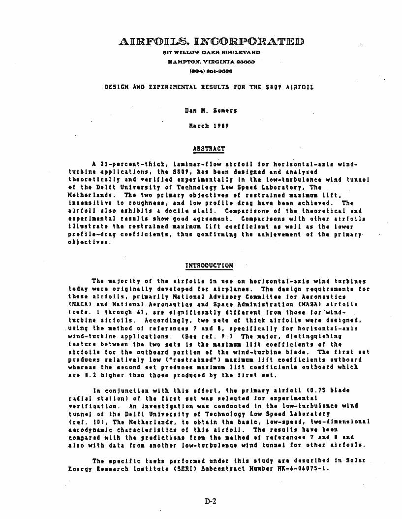
AIRFOIL§). ][NOORPORATED61T WILLOW OAKS BOULEVARD
RAMPI'ON. VIRGIlinA a3600
(1104) .1-9338
DESIGN AND EXPERIMENTAL RESULTS rOR THE sao, AIRFOIL
Dan M. SO.lrs
larch un
ABSTRACT
A Zl-perc.nt-tblck, la.lnar-flow airfoil for horllontal-aal. wlndturbln. application., the sao,. ha. bl.n d•• lvn.d and analyl.dthlor.tlcally and ••rlfl.d 'Ip.rl••ntally In lh. low-lurb.l.nc. wind tunnelof th. D.lft Unh.rslt, of T.chnolog, Low Spud Laboratory, Th.Nlth.rland•. Thl two prl.ar, ob'.ctl ••s of r •• traln.d .all.a. 11ft,In ••n.lti •• to roughnls" and low profl1. drag ha •• b••n achi'.ld. Theairfoil al.o elhlblt. a docl1 •• tall. Co.parl.on. of th. th.or.tlcal and••p.rl.ental r ••ult••how·good agr ••••nt. Co.part.on. with oth.r airfoil.111u.trat. thl re.traln.d .aal.ua 11ft co.fflcl.nt a. will a. the 10w.rprofll.-drag co.fflcl.nt •• thus conflr.lng the achl •••••nt of the prl.ary"ob'ecthes.
INTRODUCTION
Th••• ,orlty of the airfoil. In a.e on borllontal-aal. wind lurblne.today w.re originally .e•• loped for airplane.. The de.lgn requlr •••nt. forth••• airfoil •• prl.arll, National Ad.l.ory Co..ltt •• for A.ronaallc.(NACA) and National A.ronaatlc. and Spac. Ad.lnl.tratlon (NASA) alrfol11(refs. 1 throagh U, art .1gnlficantl, dlfftrtnt fro. thou lor 'wl ndturbln. airfoils. Accordingly. two .It. of thick airfoil. wlrl d•• lgn.d,
. a s i n, the •• thod of rlflrencls 7 and •• ,plcifically for horllontal-alllwind-tarblne application•. (511 rlf. ,.) Th. aa'or, di.tlngai.hingf •• tur. betw••n the two •• t. il the aaliaaa 11ft co.fflci.nt. of the~lrfolll for the oatboard portion of the wlnd-turbln. blad.. Th. flr.t I.tproduc•• r.l.tl •• l, low (-r •• trained-) .aal.ua 11ft eo.fflcl.nt. oatboardwhereal the .Icond I.t produci' .a.lau. lift co.ffici.nt. outboard whichare a.z hlghlr than tbol. produc.d b, thl fir.t I.t.
In con'unctlon with thl••ffort, the prlaary airfoil (0.7S blad.radial Itatlon) of thl flr.t •• t was ••1.ct.d fOf ••p.rl••ntal•• rlflcatlon. An In."tlgatlon wa. conduct.d in the low-tarbal.nc. windtunnel of the Delft Unl•• r.lty of T.chnolo,y Low Sp••d Laboratory(rd . 10). Th. N.thuland•• to obtain the baslc, loW-lp••d, two-dl••n.tona1a.rod,namic charact.ri.tlc. of this alffoi1. Thl r ••alt. ha•• b••nco.pared with th. pr.dlctlon. fro. th••• thod ot r.f.r.nci. 7 and. anda1.0 with data fro. anoth.r low-tarbal.nc. wind tann.l for oth.r alrtoll •.
Th. Ip.clflc taskl p.rfor••d andlr thl•• tady art dl.crlbld in ·SolarEner,y Re5.arch In.tltat. (SERI) Subcontract Na.blr HI-6-0607S-1.
D-2

EIPERI"ENTAL PROCEDURE
WIND TUNNEL
Thl low-turbulinci wind tannll (rlf: 10) of thl Dilft Uni.lrlity ofTlchnology Low Sp'ld Laboratory, Thl Nlthlrland., 1. I ClO.ld-throlt,11.011-return, at.olphlrlc tunnll tflg. 3). Thl turbulinci 11•• 1 in thlt.lt I.ction .arl •• froa J.D~ p.rclnt at 10 .1. (33 ft.I.) to 0.04 p.rclntat 60 .,. (200 ft.II).
Th. octagonal t.lt I.ctloa 1. 110.0 ca (7D.17 In.) wid. by 125.D e.(4'.21 In.) high. Ellctrically actaatld tarntablll pro.ldl pOlltloninq IDdIttachalnt for thl two-dl.lnllonl! aod.l. Th. tarntahl •• ar. flush withthe top Ind botto. tunn.l Willi Ind rotltl with thl .od.l. Thl ali. ofrotltlon colncldld with thl quart.r chord of the aod.1 which wal .ountld.Irtlcally bltw.ln the tarnta~I••. CSII fig. 4.) Thl 9api bltw.ln thl.odel Ind the turntlbll. wlrl ••al.d.
KDDEL
Th. Ila.lnua, wlnd-tannll aodll WI. conltruct.d b, the D.utlchlForlchungl- und Vlrlach.lnstllt fair taft- und lavaflhrl •. v. (DrVLR),Braun.ch•• lg, Fldlral R,publlc of Glraany. Thl aod.l had a chord of'00.10 •• (~3.'~~ In.Joand a .pan of 1~41 _ (.'.13 In.L Chordwl ••orlflc•• wlr. loclt.d in the upp.r Ind low.r lurfac'l to on. Iidl of the.ld.pln at lh. Itlgg.r.d pOlltlons 11st.d In·tabl. III. Spanwll' orlfie.sw.rl locatld In thl upp.r larfaci only In ordlr to aonltor lh. two-di.I•• Ionlllty of the flow It hl0h anolll of attact. All the oriflc'l vlre0.4D .. (0.01' In.) In dll•• t.r with thllr a••• plrp.ndlculaf to thesurflCI. Thl a.llur.d aod.l contoar wa. o.nlrally within 0.1 a.(0.004 In.) of lh. prl.crib.d shap•.
VAlE RAIE
A total-pr'llur., • Italic-pr •••ur., and an I~t.grlting watl flteWlrl aountld on I Itrut •• tw.en thl tunnll Ildlwalll (figl. 4 and 5). ThlItrut coald bl po.ltlon.d Ipanwil' and .tr.aawill in thl tl.t I.ction.Mo••••nt of thl .trut ,ro,lded pOlltlonlno of the watl rat •• noraal to thlIldlwalll. Th. tip. of thl total-pre••ar. tub'l wire locatlddown.tr.a. of thl trailing Id91 of the .odll. Thl d.tail. of thl watlrat •• arl Ihown In flgur •• , Ind 7. Thl lnt.,ratln, wat. rat. WI. not ulldin thl. in.l.tlgatlon.
INSTR1R'1ENTAT I ON
"11.arl••ntl of thl basle tunn.l prlssar.l, the Itatic prlssurl. onthl aodll lurfacl., and the watl-ratl prls.ar.1 were aade by a aultitub.aaDo•• tlr whleh was read .aato.atically a.lng photoel.ctric cIIII. Datiwlr. obtaln.d and record.d by an Illctronlc dala-acqaisltlon IYlt ••.
D-3

KETHODS
Thl .tatic-prlssurl •• asur •••nt. on thl .odll surface were reducld to.tandard prl••url cOlfficilnt. and nU.lrically intlgratld to obtain .ectionnormal-force coefficients and section pitehing-ao.ent coefficients aboutthl quarter-chord point. Section profil.-drag coefficients were computedfroa the wake-rake total and .tatic pressures by the method ofreflrencl 11. Standard, low-Ipe.d, wind-tunnll boundary corrections(ref. 13) ha., beln applied to thl data. Thl folloWing procldurl was used.
The uncorrect.d for~., aoa.nt, and prl.sarl cOlffici.nt. are r.f,rrld toth. apparent dynamic pressurl as ••asur.d tunnel ••pty at the .odllposition. Th. lift, profil.-drag, pitching-aoment, and airfoil pressurecoefficients and the angl. of attack art th.n corr.et.d by the aethod ofr.ference 13. Thl corrlctld .alaes arl plottld. Finally, as a check, thecorr.ctld airfoil pr.s5url distribution is nU.lrically intlgrated to obtainth. eorrlcted nor.al-forc. (and pitching-aoaent) cOlffici.nt which,toglther with the correctld profil.-drag co.fficilnt and angl. of attack,yi.1ds the corr.ct.d 11ft cOlffl~lent (and chord-fDrc. co.fflcilnt).
At high ang II. of·· a t tack, thl wah b.co... widlr than the wake rake.Vh.n this occurs, the drag is obtain.d fro. a parabolic •• trapolation ofthe aeasurld watt prlslur.s. At 1.ln highlr ang1.s of attack, the totalprelsurl co.fflclent••Ia.ur.d In the watt blco•• n.gati •• , .ating .calculation of the drag i~polsibl.. In thIS' cas.s, an uncorr.ctedprof ill-drag co.fficl.nt of 0.3 (.sti.at.d froa rlf. 14) is alsumld.
TESTS
Thl aod.1 was t.stld at R.ynolds nu.b.rs bas.d on aJrfoll chord froa1,000,000 to 3,000,000. Thl .od.1 wa. tlst.d s.ooth (transition frel) andwith transition fi.ld by roughn.ss at 1.02c on thl upplr surfacI and 0.05con the low.r surfac.. Thl grit roughnlss was liSld by the •• thod ofrlferencI 15 and spars.1y distributld along 3-.. (O.l-ln.) wide Itrlpsapplied to the aode1 with lacqu.r. (SI. tabl. IV.)
Starting froa lero degrels, thl angll of attack was increasld untilthe .ntire upp.r surfacI was slparatld and th.n d.crlasld In order tod.termine hysterlsil. Th••a•• proc.durl was follow.d for the nlgati.1ang1 •• of attack. For the R.ynold. nuablrs of 2,500,000 and 3,000,000, the.tatic prlssarl. on thl upp.r lurfac. could not b•••asur.d by the.anoa.ter at high angl.1 of attact b.caul. the diff.r.nc.1 b.twe.n thai'pr.ssur.s and thl fr ••-str.a. static pr ••sur. wlr. too gr.at.
For •••• ral t.st runs, thl _odll lurface. w.rl coatld with oil todetermin. the location. al well al the natur., of the boundary-lay.rtransition froa laainar to turbulent flow (r.f. 16). Tran.itlon was alsolocated using a probe containing a .icrophonl, which was positioned nearthe llading Idge and then aO.ld .lowly downstr.a. along the aod,l .urflce.Two span stations. corrllponding to the watl-rakl position and thlchordwisl orificl row, wert lur.lyed. The beginning of the turbulentboundary layer wal d.t.ct,d II an incr •••• in noill 1••• 1 o.lr that for the1aainar boundary lay.r which wal '5~lntial1, si1lnt. (SI. ref. 17.)
D-4

Two turbulator., li9-lag tap. (rlf. tl>, wI.rl placid on thl model,one betweln O.43c and O.4'c on thl upplr .urfaci and thl other betwllnO.42c andO.44c on the low.r surface, In ord.r to detlrminl their efflct onlaminar s.paration b~bbl.s and s.ction characteristics. The d.tairs of the0.2'-a. (O.DtO-ln.) thict tape are Ihown in the followin9 stitch.
J_-.A.I ''''ftI1
PRESENTATION OF RESULTS
Thl principal r.lult. of thl. In.lstigation arl prlslntld in thlfollowing fi9urls:
PreSlurl distributions for R • 2,000,000. Arrows indicatl dir.ctionof angl.-of-attack chang. (for dltlr.inatlonof hyst.rlsi.)
Oil-flow photographl of upplr lurfaci for R • 1,000,000Oil-flow photograph. of upplr lurfaci for R • 2,000,000Oil-flow photographs of upp.r surfaci for R • 3,000,000Oil-flow photographl of lowlr lurfaci for R • l,aOO,ooo ....Oil-flow photographs of lowlr lurfac. for R • 2,000,000Oil-flow photographs of lowlr lurfaci for R • 3,000.000 ....Transition location. Bar. I.tlnd fro. b.ginning ~o .nd of
transition. . . . . . . . .. . •..•Spanwisl drag co.fflcl.ntl for R • 2,000,000 ..Section eharactlrl.t(cs .....•...Effect of roughnll. on Iletion charaetiristici ..Eff.ct of ·.turbulators on drag cOlfflcilnt. . . . . ...Efflct of turbulator. on .'lction charact.ristici for R • 1,000,000 .Co.parllon of theorltical and I.plrl••ntal prll.url di.trlbutionsCo.parllon of th.oriticiland I.plri.lntal 'Ictlon charlctiriitici
with trlnsltion frel ...............•.......Co.plrl.on ofthlor.tlcil and I.plri.lntal ••ctlon charactlri.tlc.
with tran.ltion fi.ld .. . . . . . . . . . •. . .Co.parllon of .Ictlon chlractlriltlcs of SI09 and NACA 4421 airfoil.
for R • 3,000,000 ..•..•....•......•...Comparl.on of s.ction charactlrl.tic. of SI09 and NACA 23021
airfoil. for R • 3,000.000 ..••..••.••......
D-S
Fi9ure
I,101 t121314
IS161711192021
22
23
24
25


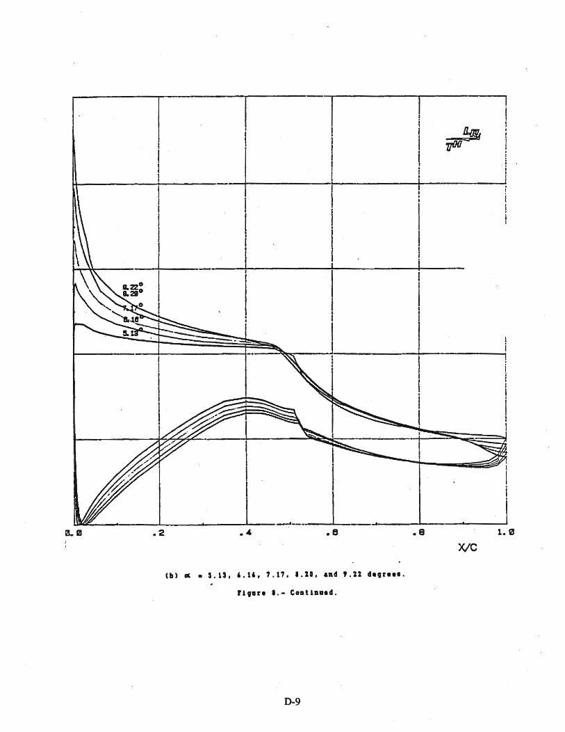

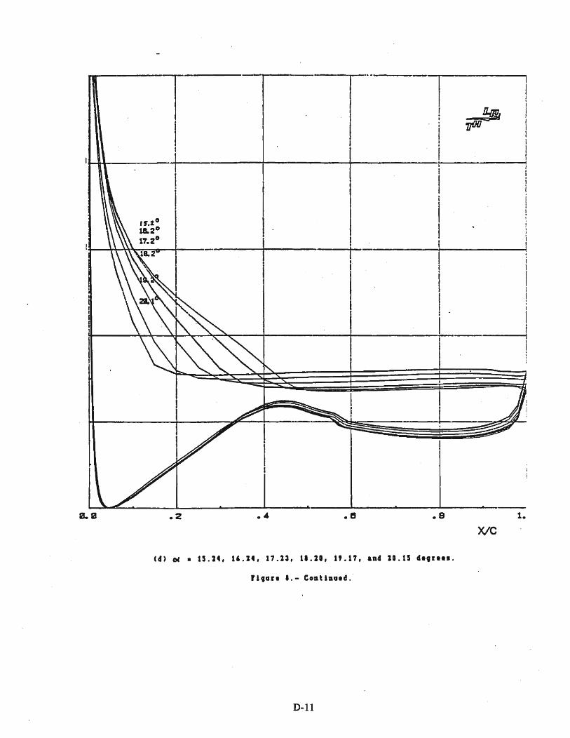

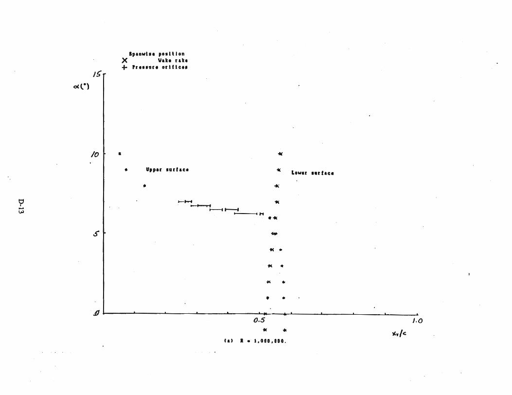

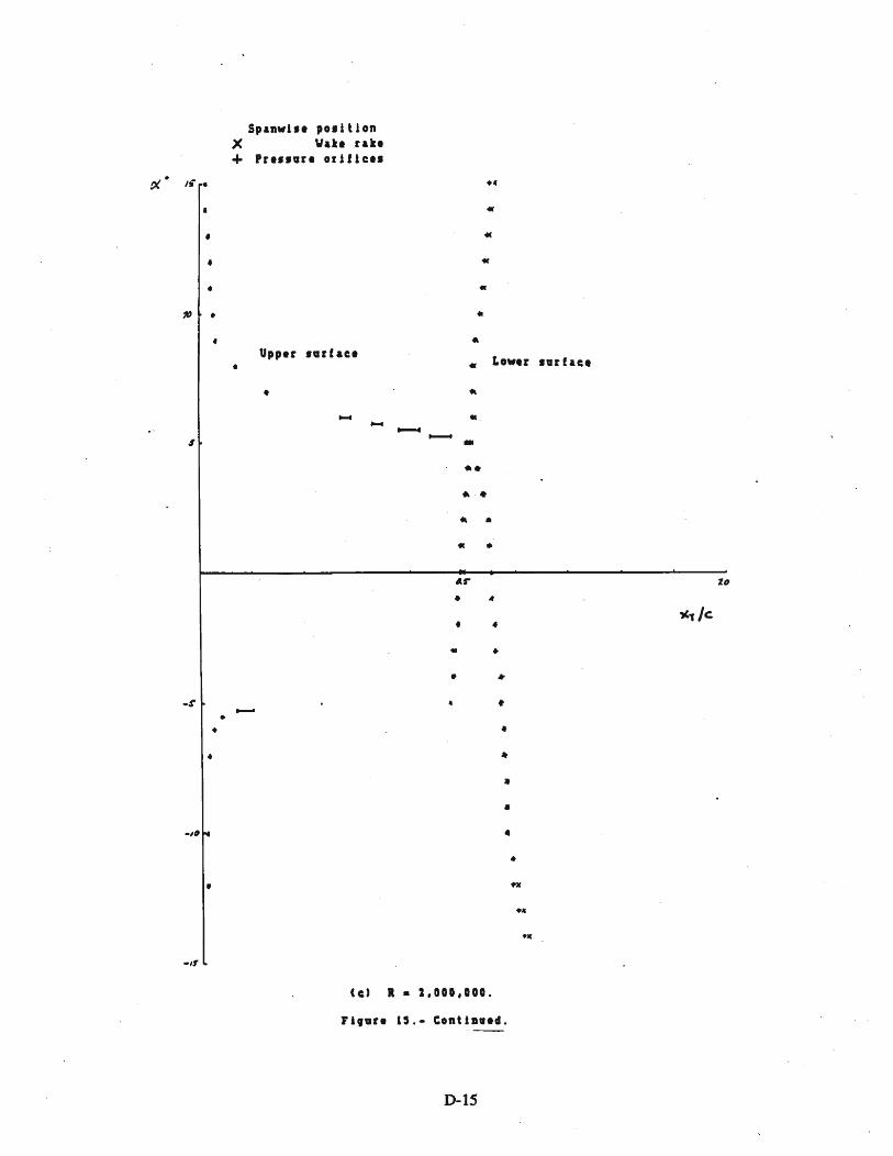
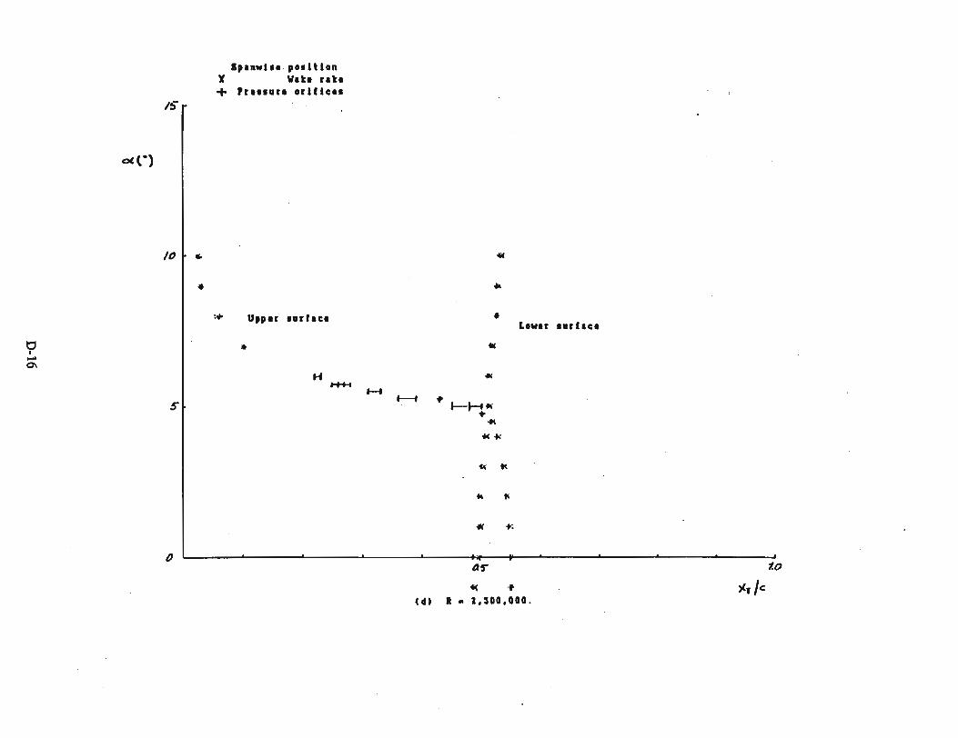
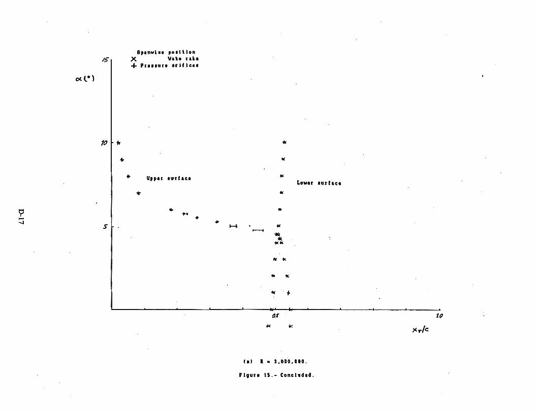

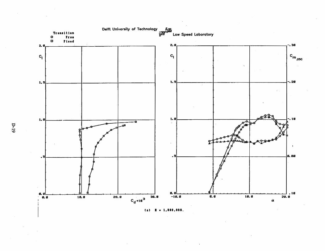

Appendix E
Wind Tunnel Tests of the 8809 Airfoil Model
E-l

T . H . E
OHIOSlATEUNIVERSITY
Aeronautial and AstronauticalResearch Laboratory
WIND TUNNEL TESTS OF
THE S809 AIRFOIL MODEL
G. M. GREGOREK
M. J. HOFFMANN
K. E. KULH
2300 West Case RoadColumbus.OH 43235-1949
Phone 614-292-5491
THE AERONAUTICAL & ASTRONAUTICAL RESEARCH LABORATORY
THE OHIO STATE UNIVERSITY
COLUMBUS. OHIO
APRIL 1991
Prepared for: SOLAR ENERGY RESEARCH INSTITUTEMIDWEST RESEARCH INSTITUTECONTRACT XL-9-19011-1
E-2

FOREWARn
This is the. Final Report on Midwest Research Institute GrantXL-9-19011-1 Entitled ''Wind Tunnel Testing on the 8809 Airfoil Model".(OSU Research Foundation Project 721623). Hr. Sandy Butterfield wasthe Technical Monitor for the Solar Energy Research Institute for theperiod November 1988 to June 1989.
E-3

TABLE 01' CONTENTS
ABSTRACT
I. INTRODUCTION
II. RESEARCH PROGRAM
A. Test Program
B. Experimental Facilities
C. Data Acquisition And Reduction
III. RESULTS AND DISCUSSIONS
A. Steady State Test Sequence
B. Vane Calibration
C. Unsteady Vane Measurements
IV. SUMMARY
APPENDICES
E-4
page
iii
1
3
3
3
5
6
6
8
10
12
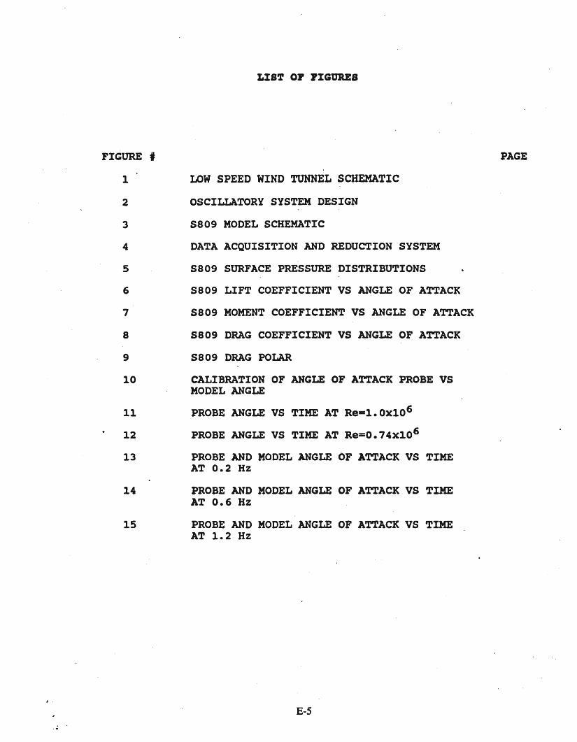
I ·
FIGURE j
1
2
3
4
5
6
7
8
9
10
11
12
13
14
15
LIST ·OP PIGURES
LOW SPEED WIND TUNNEL SCHEMATIC
OSCILLATORY SYSTEM DESIGN
5809 MODEL SCHEMATrC
DATA ACQUISITION AND REDUCTION SYSTEM
S809 SURFACE PRESSURE DISTRIBUTIONS
S809 LIFT COEFFICIENT VS ANGLE OF ATTACK
S809 MOMENT COEFFICIENT VS ANGLE OF ATTACK
S809 DRAG COEFFICIENT VS ANGLE OF ATTACK
S809 DRAG POLAR
CALIBRATION OF ANGLE OF ATTACK PROBE VSMODEL ANGLE
PROBE ANGLE VS TIME AT Real.OX106
PROBE ANGLE VS TIME AT Re=O.74xl06
PROBE AND MODEL ANGLE OF ATTACK VS TIMEAT 0.2 Hz
PROBE AND MODEL ANGLE OF ATTACK VS TIMEAT 0.6 Hz
PROBE AND MODEL ANGLE OF ATTACK VS TIMEAT 1.2 Hz
E-5
PAGE
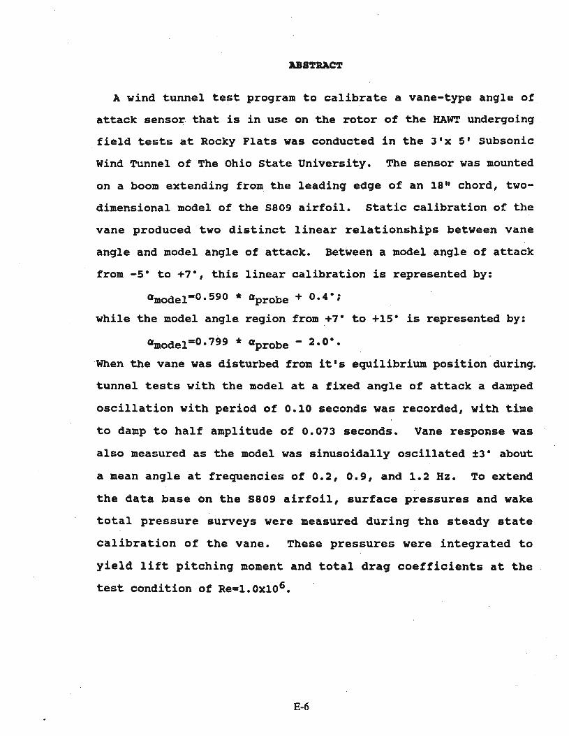
ABSTRACT
A wind tunnel test program to calibrate a vane-type angle of
attack senso~ that is in use on the rotor of the HAWT undergoing ,
field tests at Rocky Flats was conducted in the 3'x 5' Subsonic
Wind Tunnel of The Ohio state University. The sensor was mounted
on a boom extending from the leadinq edge of an 18" chord, two
dimensional model of the S809 airfoil. static calibration of the
vane produced two distinct linear relationships between vane
angle and model angle of attack. Between a model angle of attack
from -5· to +7-, this linear calibration is represented by:
Qmodel=0.590 * Qprobe + 0.4-;
while the model angle reqion from ,+7 - to +15- is represented by:
Qmodel=0.799 * Qprobe - 2.0-.
'When the vane was disturbed from it's equilibrium position during.
tunnel tests with the model at a fixed anqle of attack a damped
oscillation with period of 0.10 seconds was recorded, with time
to damp to half amplitude of 0.073 seconds. Vane response was
also measured as the model was sinusoidally oscillated ±3- about
a mean angle at frequencies of 0.2, 0.9, and 1.2 Hz. To extend
the data base on the S809 airfoil, surface pressures and wake
total pressure surveys were measured durinq the steady state
calibration of the vane. These pressures were integrated to
yield lift pitchinq moment and total draq coefficients at the
test condition of Re=1.0xl06•
E-6

I. INTRODUCTION
The 5809 airfoil is an airfoil tailored for Horizontal Axis
Wind Turbine (HAWT) rotors. It is presently being used on the
HAWT at Rocky Flats and .i s undergoinq extensive field tests.
This rotor on the field test machine has a vane projecting from '
the leading edge of the airf~il to 'be used as an anqle of attack
measuring device. The upwash from the airfoil alters the flow
field of the vane, necessitating a calibration .of the vane versus
model angle of attack. The purpose of the experimental program
conducted at the Aeronautical and Astronautical Research Labora
tory (AARL) of The Ohio state University (OSU) reported here, is
to provide this calibration for both steady and unsteady flow
conditions. In addition, during the steady state tests, surface
pressures are obtained and wake pressures measured to supplement
the existing data base on the aerodynamic characteristics of the
S809 airfoil.
The OSU 3 1x 51 Subsonic Wind Tunnel was used for the test
program. Test conditions were at a Reynolds number of 1x10⁶
based on an 18" model chord. Steady state pressures were meas
ured at angles of attack from.-S- to +15- and were reduced to
lift and pitching moment coefficients_ A wake survey probe
provided total drag for the steady state test sequence. Unsteady
information was obtained by 'oscillating the model with a sinusoi
dal wave form of amplitude ±3-. During the oscillations both
vane angle and model angle of attack were recorded. These data,
coupled with the steady state calibration of the vane versus
model angle of attack provide the needed calibration.
E-7

A description of the e~perimental program, wind tunnel and
model, fabricated earlier from the same mold ·used to produce the
HAWT rotor being field tested, follows. Results of the test are
presented in .both tabular and graphic form and include a short
test sequence of the dynamic response of the vane. An Appendix
includes the airfoil coordinates and location of the pressure
taps on the model to complete the report.
&8

II. RESEARCH PROGRAK
A. Test proqram
The main purpose of the present test program was the calibra
tion of the angle of attack vane relative to the airfoil angle of
attack. These calibrations were to be performed in steady state
and in an unsteady condition with the airfoil oscillating sinu
soidally at a nominal ±3- angle of attack. During the steady
state tests, surface pressures were to be recorded as well as
airfoil and vane angle of attack to provide pressure distribu
tions which could be integrated to lift, moment and pressure drag
coefficients. A wake survey would also be conducted to determine
the total drag of the airfoil. These steady state data were to
supplement data obtained from the model in an earlier test ser
ies.
All tests were conducted at a nominal Reynolds number of 1xl06
based on the 18" model chord.
B. Experimental Pacilities
The Subsonic Wind Tunnel at AARL is shown schematically in
Figure 1. It is an open-circuit, atmospheric wind tunnel of the
Eiffel type, powered by a 125 hp AC motor driving an 8' diameter,
6 blade fan. · The blade angle can be set, manually, to produce
velocities from 20 to 200 ft/sec. Test section turbulence level
is low; four 40 mesh seamless stainless steel screens and a 4
inch thick honeycomb of 1/4 inch cells upstream of the contrac
tion maintains' a turbulence level measured below 0.1%_·
The test section geometry is rectangular, with filleted cor
ners; dimensions of the test section are 55" wide and 39" high.
E-9

Because of ' this .or i ent a t i on , two dimensional airfoil models are
mounted vertically in the facility. A horizontally traversing
single total pressure probe is used to survey the wake behind the
airfoil to measure total airfoil drag • . Wind tunnel test condi
tions are monitored by a single total probe mounted off the wall
and by two static ports mounted in each side wall as shown in the
schematic.
Two pressure sensing systems can be used to measure airfoil
pressure distributions. For steady state measurements a single
pressure transducer is coupled to a 48 port scanning system
located outside of the wind tunnel to make the surface measure
ments. When unsteady pressure are required, two electronically
scanned pressure modules can be mounted inside the model to
reduce the length of pressure tubing and to provide the necessary
rapid response.
These unsteady airfoil tests are performed on pressure tapped
airfoil models mounted on the oscillating rig shown in Figure 2.
The rig is driven by a 5 hp AC motor that is controllable over a
wide range of frequencies. Because large airfoil models are
being studied, frequencies from 0.1 to 2 Hz are pertinent for the
wind turbine applications of interest. Amplitude and wave form
during the oscillation are controlled by specially designed face
cams. Sinusoidal wave forms and other more complex wave shapes
are available.
The two dimensional model of 18" chord studied in this experi
mental series has the specially designed S809 contour. It's
coordinates are listed in Table I of the appendix. Table II in
the appendix gives the location of the 31 pressure taps used in
the steady state surface pressure measurements. A sketch of the
&W
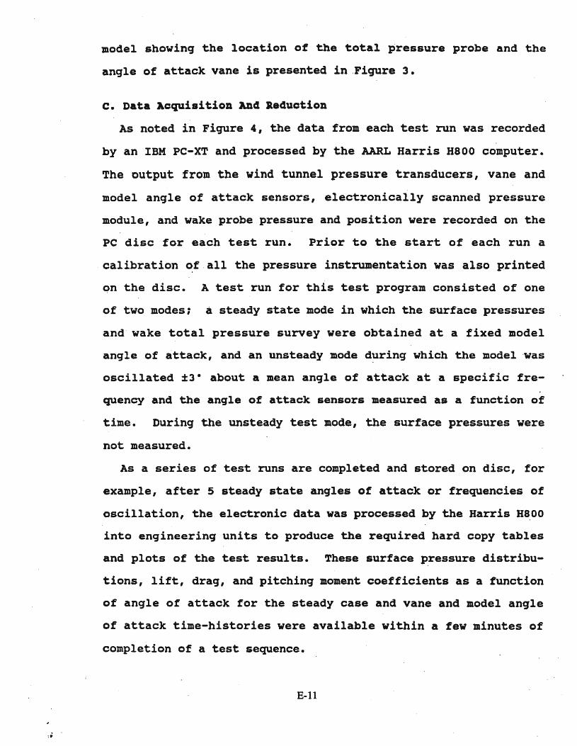
model showing the location of the total pressure probe and the
angle of attack vane is presented in .Figure 3.
c. Data Acquisition ADd Reduction
As noted in Fiqure 4, the data from each test run was recorded
by an IBM PC-XT and processed by the AARL Harris Haoo computer.
The output from the wind tunnel pressure transducers, vane and
model angle of attack sensors, electronically scanned pressure
module, and wake probe pressure and position were recorded on the
PC disc for each test run. Prior to the start of each run a
calibration ~f -all the pressure instrumentation was also printed
Qn the disc. A test run for this test program consisted of one
of two modes: a steady state mode in which the surface pressures
and wake total pressure survey were obtained at a fixed model
angle of attack, and an unsteady mode d~ring which the model ·was
oscillated ±3- about a mean angle of attack at a specific fre
quency and the angle of attack sensors measured as a function of
time. During the unsteady test mode, the surface pressures were
not measured.
As a series of test runs are completed and stored on disc, for
example, after 5 steady state angles of attack or frequencies of
oscillation, the electronic data was processed by the Harris H~OO
into engineering units to produce the required hard copy tables
and plots of the test results. These surface p~essure distribu
tions, lift, drag, and pitching moment coefficients as a function
of angle of attack for the steady case and vane and model angle
of attack time-histories were available within a few minutes of
completion of a test sequence.
B-11
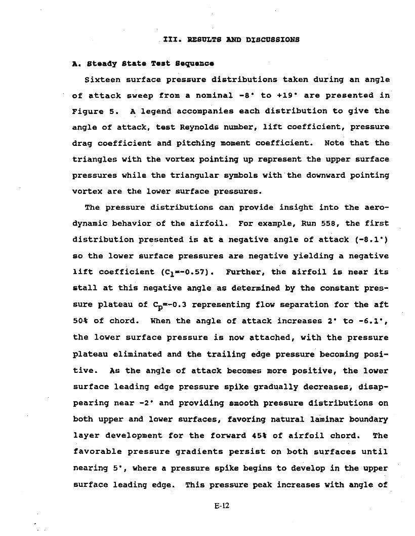
xxx_ RESULTS AND DXSCUSSXOHS
A_ Steady State Test Sequence
sixteen surface pressure distributions taken during an angle
of attack sweep from a nominal -8- to +19- are presented in
Figure 5. A legend accompanies each distribution to give the
angle of attack, test Reynolds number, lift coefficient, pressure
drag coefficient and pitching moment coefficient. Note that the
triangles with the vortex pointing up represent the upper surface
pressures while the triangular symbols with the downward pointing
vortex are the lower surface pressures.
The pressure distributions can provide insight into the aero
dynamic behavior of the airfoil. For example, Run 558, the first
distribution presented is at a negative angle of attack (-8.1-)
so the lower surface pressures are negative yielding a negative
lift coefficient (Cl=-0.57). Further, the airfoil is near its
stall at this negative angle as determined by the constant pres
sure plateau of Cp=-0.3 representing flow separation for the aft
50% of chord. When the angle of attack increases 2- to -6.1·,
the lower surface pressure is now attached, with the pressure
plateau eliminated and the trailing edge pressure becoming posi
tive. As the angle of attack becomes more positive, the lower
surface leading edge pressure spike gradually decreases, disap
pearing near -2- and providing smooth pressure distributions on
both upper and lower surfaces, favoring natural laminar boundary
layer development for the forward 45' of airfoil chord. The
favorable pressure gradients persist on both surfaces until
nearing 5·, where a pressure spike begins to develop in the upper
surface leading edge. This pressure peak increases with angle of

attack. At 7.1· the flow is attached up to the trailing edge,
but by 9.2· the flow has separated past the 55t chord of the
upper surface. In spite of this flow separation the low pressure
spike' continues to increase, with a corresponding modest increase
in lift coefficient until complete separation occurs on the upper
surface as shown at angle of attack 16.8·, and the lift coeffi
cient falls.
The integrated surface pressure distributions are presented in
Figures 6 to 9. Figures 6 and 7 'indicate the lift and pitching
moment coefficient versus angle of attack. The total drag coef
ficient obtained from integration of the momentum deficit in the
wake is illustrated in Figure 8; the pressure drag coefficient
is not shown since the pressure taps- on the model were not felt
to be sufficient to determine a reliable value of pressure drag.
A drag polar is given in Figure 9. From this information, perti-·
nent aerodynamic characteristics for this airfoil are summarized
in Table I below:
'1'ABLB I
5809 Measured Aerodynamic Coefficients At Re= 1.05 x 10⁶
Clmax 0.91 @ 0=7· , 1.03 @ 0=15·
dCl/da 0.121 '
alo -1.0
CMo -0.035
Cdmin 0.0069 @ a=5·
(Cl/Cd)mx 107 @ a=5·
-0.57 @a=-S·
E-13
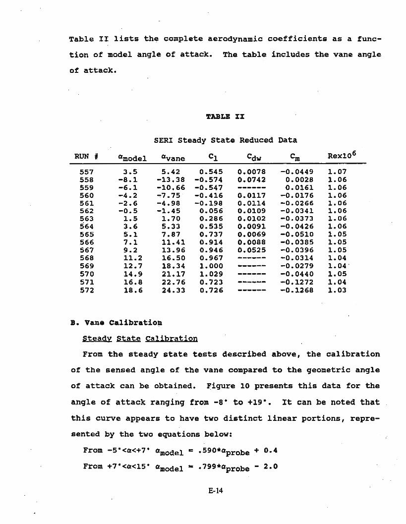
Table II lists the complete aerodynamic coefficients as a func
tion of model angle of attack. The table includes the vane angle
of attack.
TABLB XX
SERI Steady State Reduced Data
RUN tI °model °vane Cl Cdw em Rexl06
557 3.5 5.42 0.545 0.0078 -0.0449 1.07558 -8.1 -13.38 -0.574 0.0742 0.0028 1.06559 -6.1 -10.66 -0.547 ------ 0.0161 1.06560 -4.2 ~7.75 -0.416 0.0117 -0.0176 1.06561 -2~6 -4.98 -0.198 0.0114 -0.0266 1.06562 -0.5 -1.45 0.056 0.0109 -0.0341 1.06563 1.5 1.70 0.286 0.0102 -0.0373 1.06564 3.6 5.33 0.535 0.0091 -0.0426 1.06565 5.1 7.87 0.737 0.0069 -0.0510 1.05566 7.1 11.41 0.914 0.0088 -0.0385 1.05567 9.2 13.96 0.946 0.0525 -0.0396 1.05568 11.2 16.50 0.967 ------ -0.0314 1.04569 12.7 18.34 1.000 ------ -0.0279 1.04 ·570 14.9 21.17 1.029 ------ -0.0440 1.05571 16.8 22.76 0.723 ------ -0.1272 1.04572 18.6 24.33 0.726 ------ -0.1268 1.03
B. Vane Calibration
Steady state Calibration
From the steady state tests described above, the calibration
of the sensed angle of the vane compared to the geometric angle
of attack can be obtained. Figure 10 presents this data for the
angle of attack ranging from -8- to +19-_ It can be noted that
this curve appears to have two distinct linear portions, repre
sented by the two equations below:
From -5-<0<+7- 0model - .590*Oprobe + 0.4
From +7·<0<15- 0model = .799*ap r obe - 2.0
E-14

••
The two equations represent the experimental data with to.1· in
their range of applicability.
The two segment behavior of the vane calibration is related to
the loss of circulation as the flow separates from the airfoil.
Referring back to th~ pressure distributions, the angles of
attack between -5· and +7· all have positive pressures at the
trailing edge, indicating attached flow to the trailing edge and
a corresponding linear increase in lift with angle. At angles
above 7·, up to 14.9·, a low pressure plateau exists on the upper
aft airfoil surface with a leading edge pressure spike increasing
with angle. The pressure spike collapses at "16.8· and, again,
the vane calibration re~~ects this flow behavior by departing
from the linear equation. A similar separation pattern exists at
the negative angles of attack when the angle exceeds -5·, with
the vane calibrations again becoming non-linear.
Vane Response
A limited test sequence ~as per£ormed to examine the response
of the vane. With the model fixed at an angle of attack and the
tunnel operating, a clip restraining the vane was released,
allowing the vane to respond to the flow field about the airfoil.
Figures 11 and 12 illustrate the probe angle of attack as a
function of time. The vane responds with a damped oscillation as
shown. Two other trials at this wind tunnel test condition were
made, then two more such vane response checks were made at a
lower speed, corresponding to Re c O.74X106• Table III summa
rizes this response data.
~lS
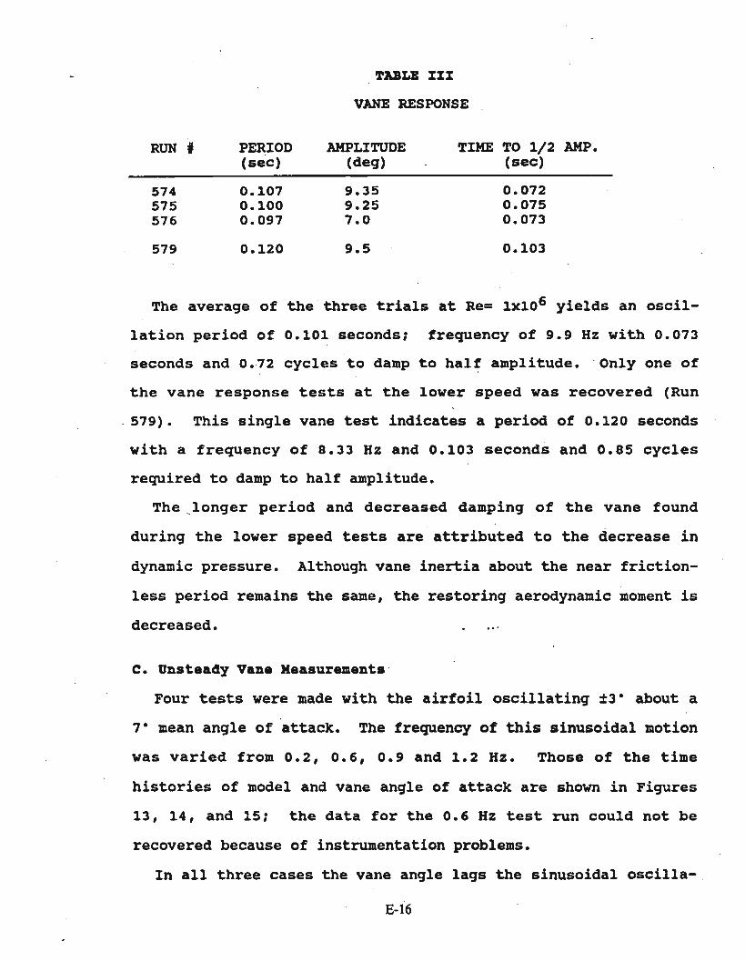
TABLB X:tJ:
VANE RESPONSE
RUN I PERIOD AMPLITUDE TIME TO 1/2 AMP.(sec) (deg) (sec)
574 0.107 9.35 0.072575 0.100 9.25 0.075576 0.097 7.0 0.073
579 0.120 9.5 0.103
The average of the three trials at Re= 1x10⁶ yields an oscil
lation period of 0.101 seconds; frequency of 9.9 Hz with 0.073
seconds and 0. ·72 cycles to damp to half amplitude • . Only one of
the vane response tests at the lower speed was recovered (Run
- 579). This single vane test indicates a period of 0.120 seconds
with a frequency of 8.33 Hz and 0.103 seconds and 0.85 cycles
required to damp to half amplitude.
The ~longer period and decreased damping of the vane found
during the lower speed tests are attributed to the decrease in
dynamic pressure. Although vane inertia about the near friction
less period remains the same, the restoring aerodynamic moment is
decreased.
c. Unsteady Vane Xeasurements
Four tests were made with the airfoil oscillating ±3· about a
7· mean angle of attack. The frequency of this sinusoidal motion
was varied from 0.2, 0.6, 0.9 and 1.2 Hz. Those of the time
histories of model and vane angle of attack are shown in Figures
13, 14, and 15; the data for the 0.6 Hz test run could not be
recovered because of instrumentation problems.
In all three cases the vane angle lags the sinusoidal oscilla-
E-16

••
. t i ons of the models. Examination of the digital data for each
test case indicates a phase lag of approximately 0.28 seconds for
the 0.2 Hz test, 0.05 seconds for the 0.9 Hz test and 0.03 sec
onds for the. 1.2 Hz case. These values for phase shift of the
vane time-history must be taken as approximate times; 'however,
since both angle of attack sensor outputs appear to"have a siza
ble noise level. The follower on the face cam that drives the
model angle of attack causes some ·chatter" in the model angle of
attack signal. When that "chatter" is coupled with the motion of
the vane that has the damped oscillation noted earlier, the vane
and model outputs are difficult to interpret.
Attempts to use the steady state calibrations of Fiqure '10 to
predict the model angle of attack from the vane output met with
mixed success. By applying the phase shift, using the static
ca~ibration and the vane measured angle, the model angle ofat~ack many times could be predicted within to.2· of the measured
model angle. At other times, the predicted values were more than
1·- off, usually due to noise in the digital output~ It appears
that a smoothing routine must be applied to the vane output to
reduce the scatter in the vane output data. As of this writing
it does appear that the static calibrations may be used to pre
dict the model angle of attack when the frequency dependent phase
lag of the vane is used to adjust prediction•

xv_ SUHKARY
A two dimensional model of the S809 airfoil has been tested in
the asu 3 1x 51 Subsonic Wind Tunnel. The experimental program
was performed to calibrate an angle of attack vane mounted on the
model and to provide additional aerodynamic data on the S809
characteristics.
Under steady state conditions, the vane angle versus model
angle resolved into two linear regions. In the model angle of
attack range from -5- to +7-,
Qmodel= 0.590 * Qprobe + 0.4
In the model angle of attack range from +7- to +15-
Qmodel= 0.799 * Qprobe - 2.0
In terms of probe angle measurements, the first equation applies
from a probe angle of -9- to +11-, the latter equation applies
when probe output is +11- to +21-. outside these angle of attack
ranges, the calibrations are non-linear.
Unsteady tests measured the dynamic response of the vane when
freed sUddenly. from a restraint while the tunnel was operating
and the model held at a ·fixed angle of attack. The period of the
damped oscillating response averaged 0.101 seconds for three
response trials at Re = lX106• Time to damp to half amplitude
averaged 0.073 seconds. At a lower Reynolds number (.74X106) a
single trial resulted in increase in both the period and half
amplitude time. A second unsteady series of tests put the model
in sinusoidal motion. The vane followed this motion, lagging the
model by approximately .28, .05 and .03 seconds for the three
recorded oscillation frequencies of 0.2, 0.9 and 1.2 HZ, respec-
E-18
tively. Application of the steady state vane calibration using
these phase laqs appeared to yield adequate predictions of model
anqle of attack for selected trials. However, both sets of
sensed.·anqle data, vane and model, require smoothinq and addi
tional analysis to improve the calibrations.
The measured steady state pressure distributions verified the
favorable laminar flow pressure gradients and the limited maximum
lift designed into the 8809 airfoil for KAWT applications. The
minimum draq coefficient measured was Cd - 0.0069, produclnq a
maximum lift to draq ratio of 107 at a - 5-. At a - 7- flow
separation occurred to initiate a limited maximum lift with full
separation from the upper surface at a - 14.9- holdinq the .maxi
mum value of lift coefficient to Cl - 1.029.
E-19
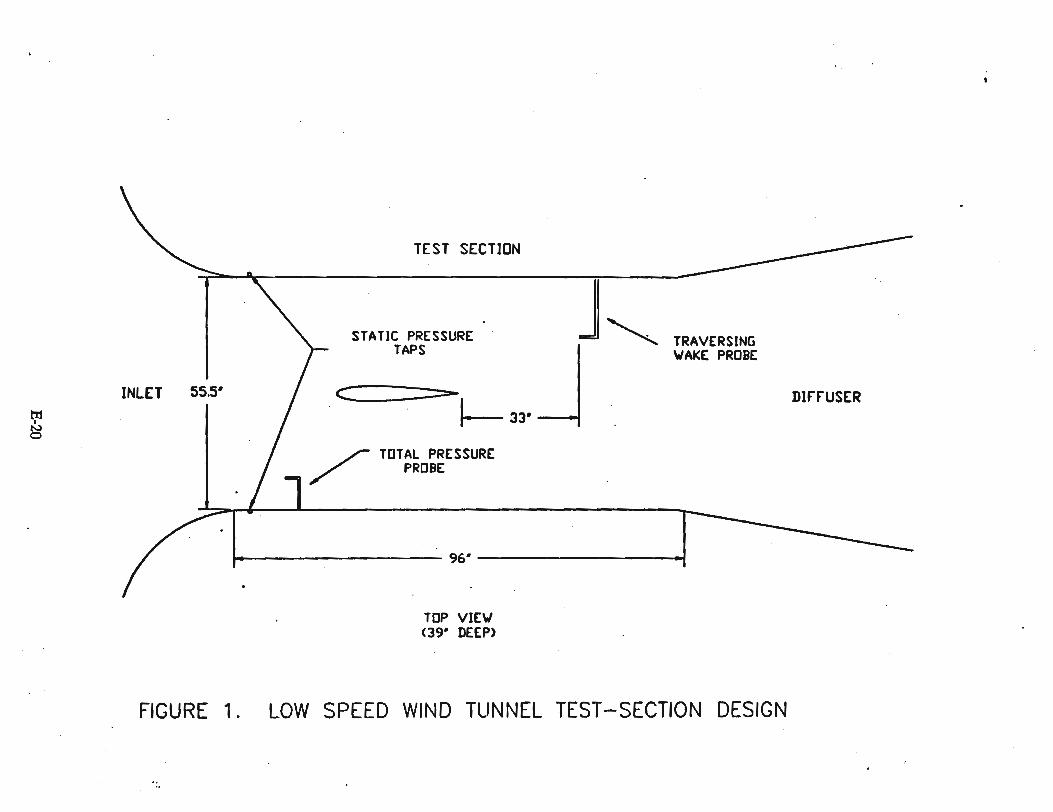

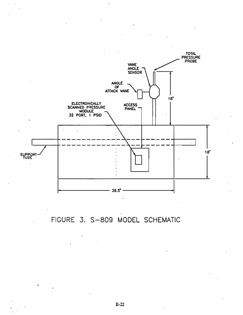

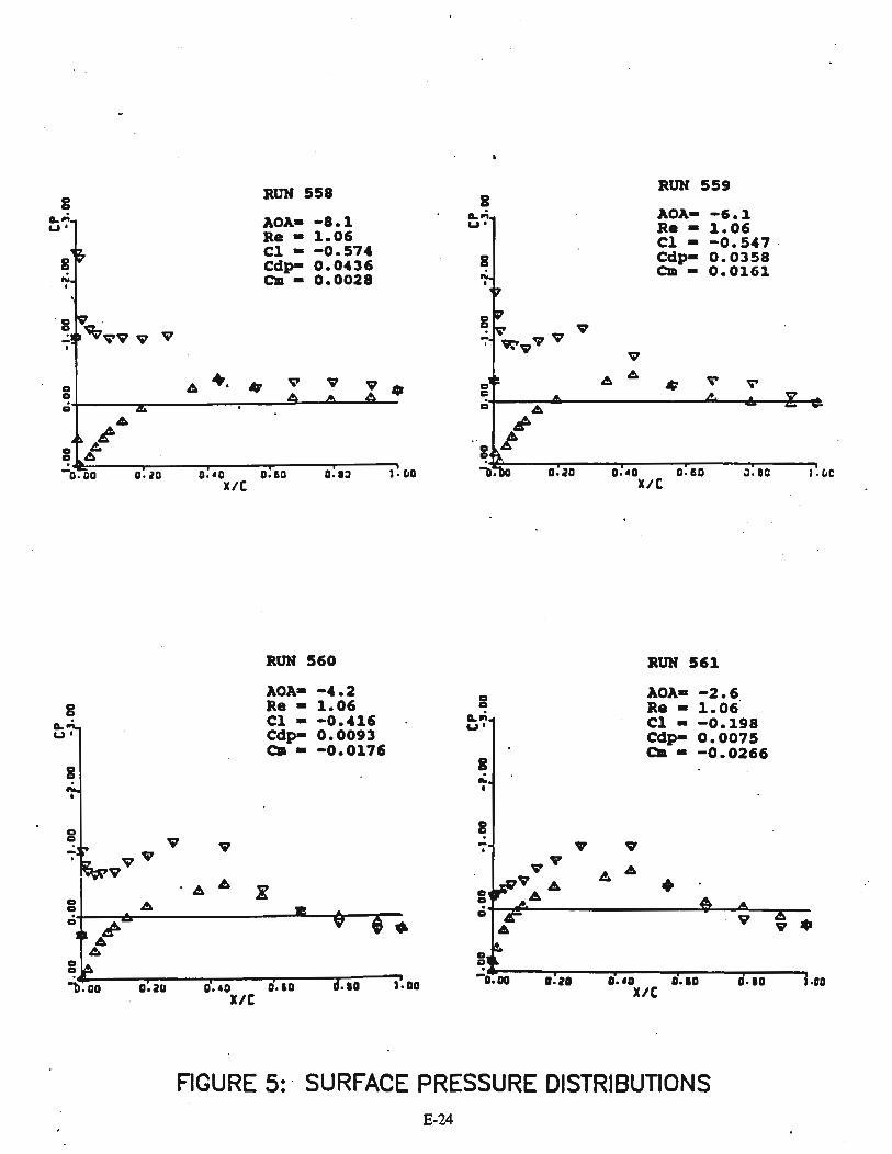
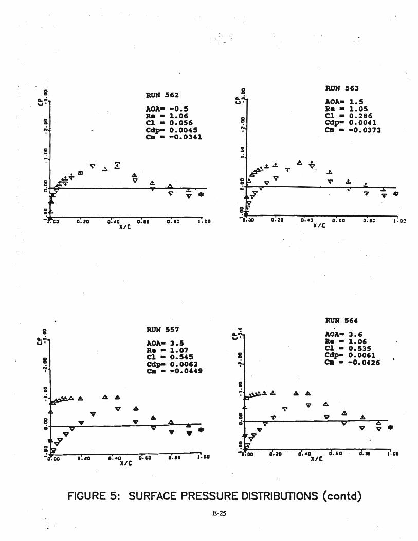


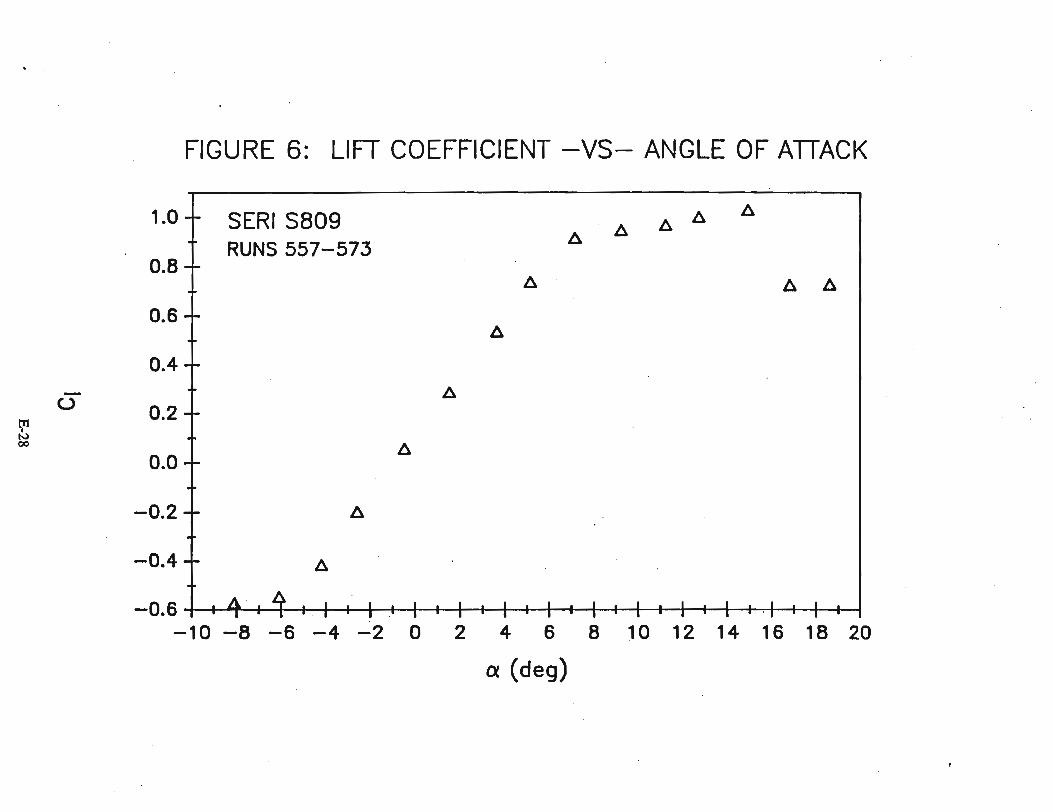
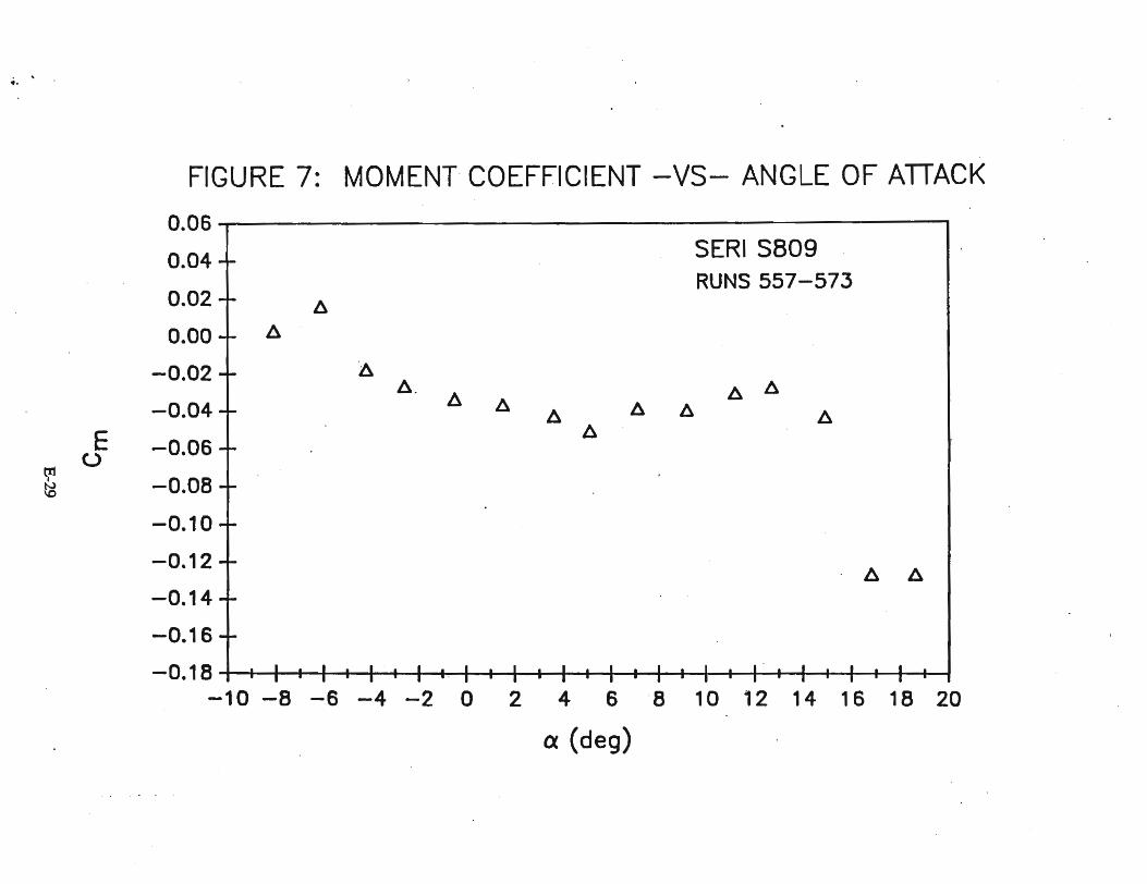
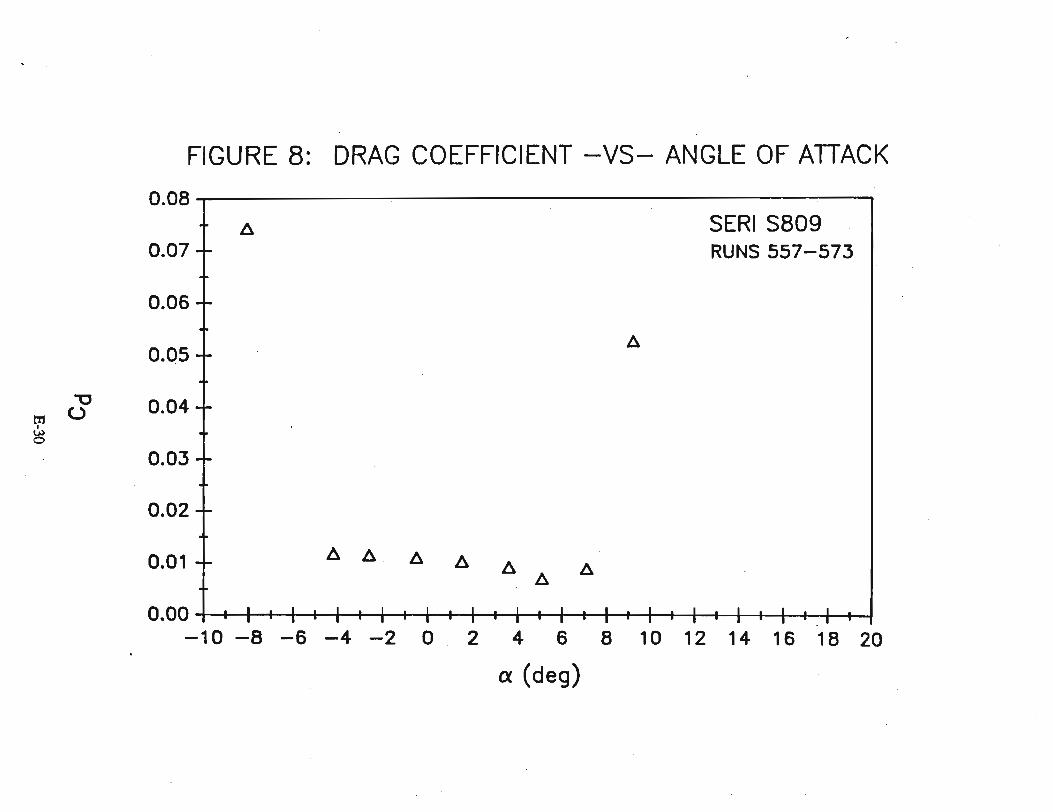

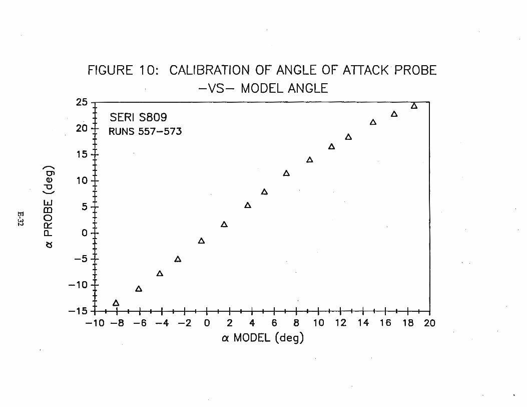


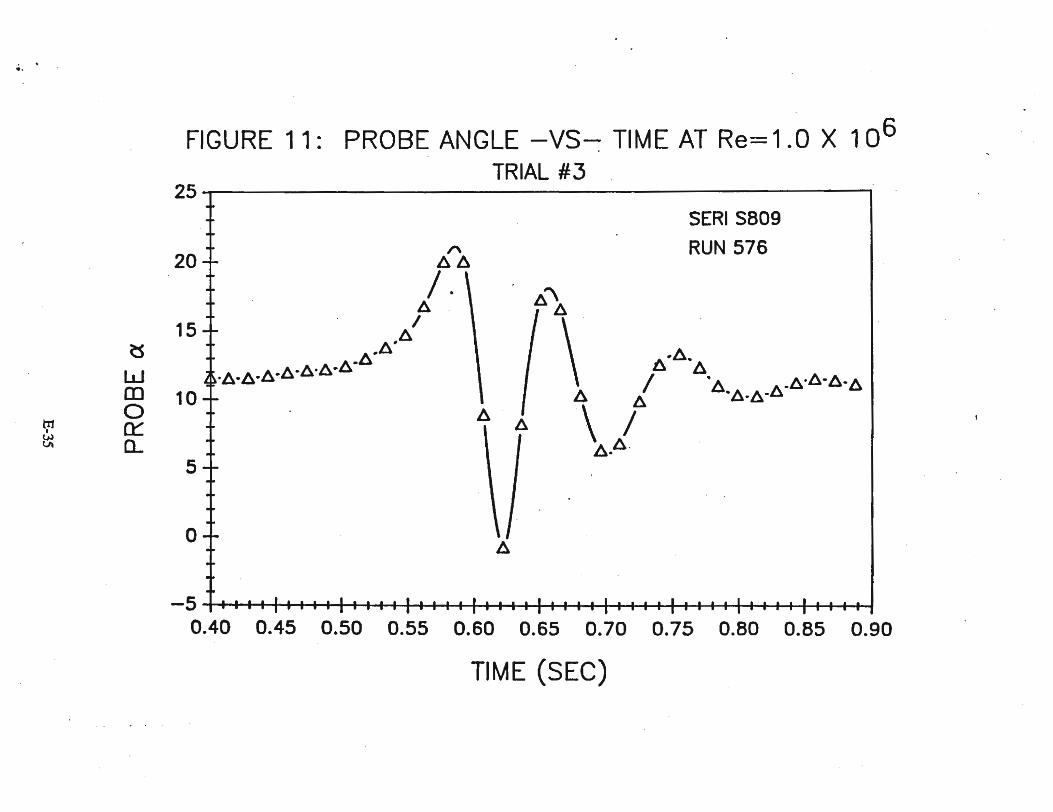
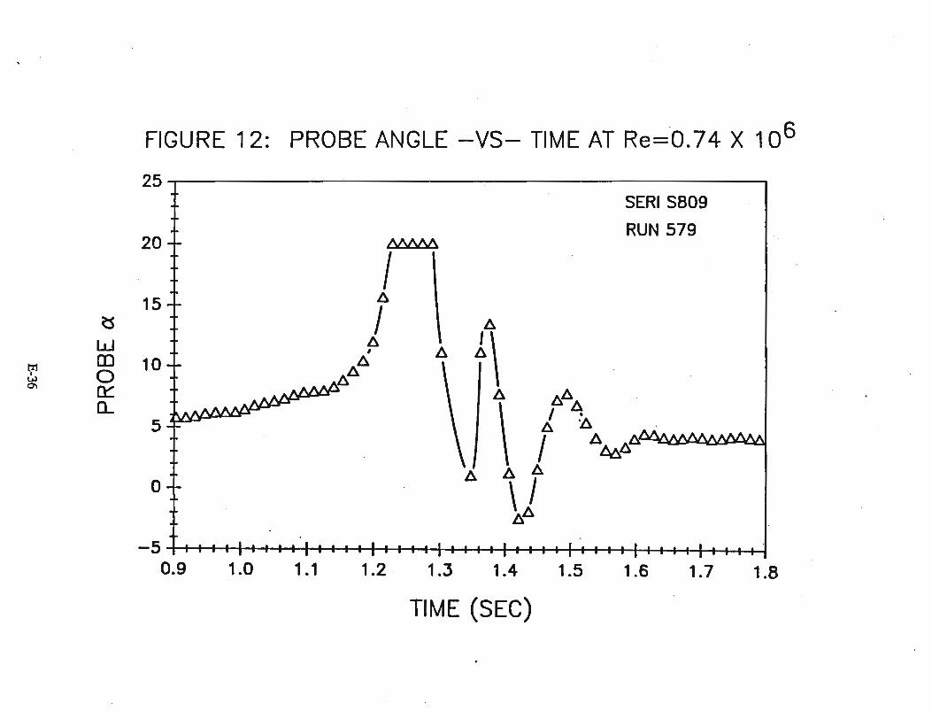
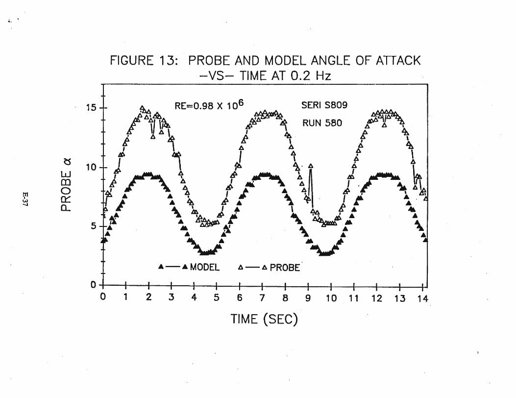


APPENDICES
E-40
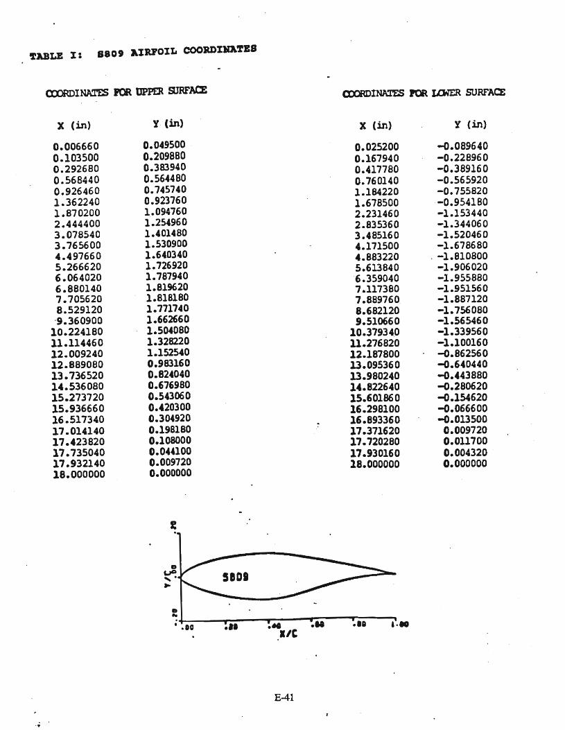
DUO, ...
• .DO .11 ... .11lIe
E-41
.Ia
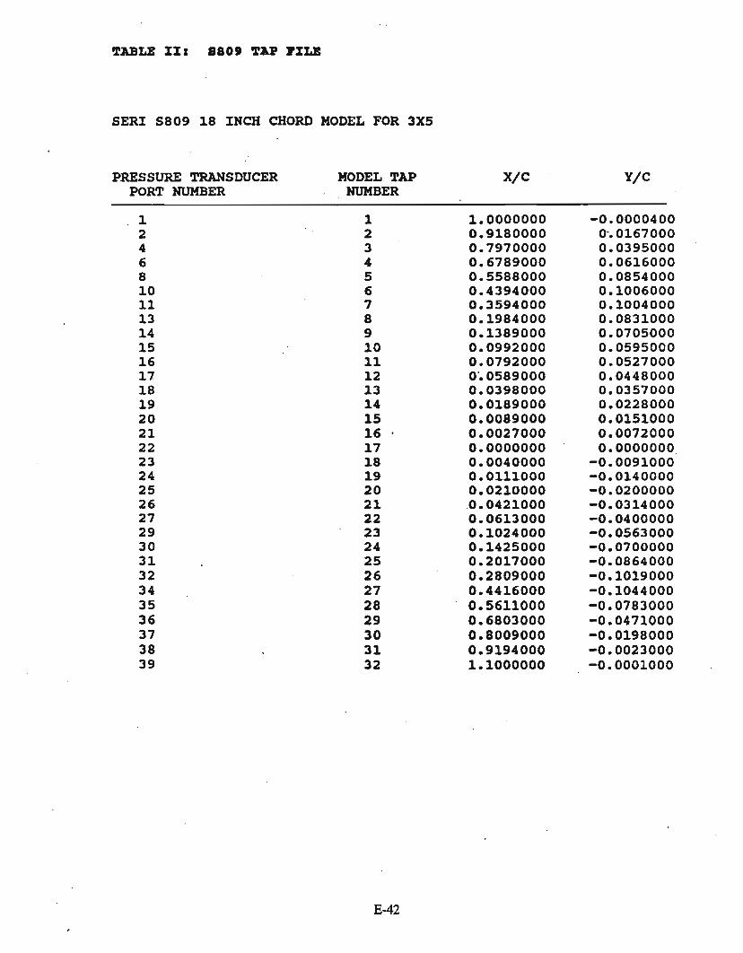
TABLE II I 880 t TAP I'J:LB
SERI S809 18 INCH CHORD MODEL FOR 3X5
PRESSURE TRANSDUCER MODEL TAP X/C Y/CPORT NUMBER NUMBER
1 1 1.0000000 -0.00004002 2 0.9180000 0-.01670004 3 0.7970000 0.03950006 4 0.6789000 0.06160008 5 0.5588000 0.085400010 6 0.4394000 0.100600011 7 0.3594000 0.100400013 8 0.1984000 0.083100014 9 0.1389000 0.070500015 10 . 0.0992000 0.059500016 11 0.0792000 0.052700017 12 0'.0589000 0.044800018 13 0.0398000 0.035700019 14 0.0189000 0.022800020 15 0.0089000 0.015100021 16 0.0027000 0.007200022 17 0.0000000 0.000000023 18 0.0040000 -0.009100024 19 0.0111000 -0.014000025 20 0.0210000 -0.020000026 21 0.0421000 -0.031400027 22 0.0613000 -0.040000029 23 0.1024000 -0.056300030 24 0.1425000 -0.070000031 25 0.2017000 -0.086400032 26 0.2809000 -0.101900034 27 0.4416000 -0.104400035 28 0.5611000 -0.078300036 29 0.6803000 -0.047100037 30 0.8009000 -0.019800038 31 0.9194000 -0.002300039 32 1.1000000 -0.0001000
E-42

Appendix F
Integrated Coefficients from all Tests
Plots of Integrated Coefficients
F-l
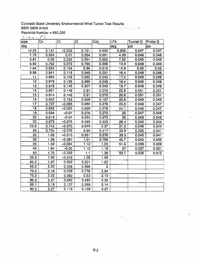
Colorado State University Environmental Wind Tunnel Test ResultsSERI S809 AirfoilReynolds Number = 650,000
alpa Cn Ct CI Cdp LFA Tunnel a Probe adeg deg psi psi
-0.25 0.151 -0.002 0.151 0.002 0.808 0.047 0.0471.75 0.354 0.01 0.354 0.001 4.09 0.048 0.0483.81 0.56 0.035 0.561 0.002 7.62 0.048 0.0485.92 0.762 0.073 0.765 0.006 10.9 0.049 0.0497.94 0.854 0.104 0.86 0.015 13.8 0.05 0.059.98 0.841 0.116 0.848 0.031 16.4 0.049 0.048
11 0.884 0.128 0.892 0.043 17.4 0.049 0.04912 0.879 0.136 0.888 0.049 18.4 0.049 0.04813 0.918 0.145 0.927 0.043 19.7 0.049 0.04914 0.901 0.148 0.91 0.075 20.8 0.051 0.05115 0.914 0.148 0.91 0.075 20.8 0.051 . 0.05116 0.922 0.153 0.928 0.107 22.9 0.049 0.04917 0.737 -0.066 0.686 0.278 23.3 0.048 0.04718 0.693 -0.065 0.639 0.276 24.1 0.048 0.04719 0.634 -0.07 0.576 0.273 25 0.047 0.04620 0.613 -0.07 0.552 0.275 26 0.048 0.04622 0.673 -0.076 0.596 0.323 28.4 0.045 0.044
23.9 0.743 -0.075 0.649 0.37 31.2 I 0.046 0.04426 0.794 -0.076 0.68 0.417 33.9 I 0.045 0.04130 1.02 -0.073 0.851 0.576 39.3 0.045 0.04135 1.28 -0.067 1.01 0.789 45.7 0.042 0.03540 1.52 -0.064 1.12 1.03 51.5 0.039 0.02945 1.64 -0.05 1.12 1.19 57 0.037 0.02150 1.75 -0.032 1.1 1.36 59.1 0.035 0.012
55.3 1.92 -0.018 1.08 1.5860.2 1.87 0.002 0.931 1.6265.2 2.22 0.038 0.968 270.2 2.18 0.039 0.776 2.0475.2 2.22 0.062 0.63 2.1380.2 2.37 0.082 0.485 2.3285.1 2.15 0.107 .0.289 2.1490.2 2.27 0.116 0.109 2.27
F-2

Colorado State University Environmental Wind Tunnel Test Resul.ts.SEAl S809 Airfoil ..Reynolds Number =500,000Smooth
. . -: . v'.: :.-,:: :.', " . ... ..".. _.. . . . .. ..
: -:.,.,., : .
. .. . . ...
alpha Cn cr CI Cdp LFAdeg deg
-2.23 -0.06 -0.004 -0.06 0.006 -2.34-0.161. 0.156 -0.005 0.156 0.004 0.8
1.84 0.369 0.005 0.369 0.006 4.133.88 0.571 0.031 0.571 0.008 7.445.89 0.752 0.068 0.755 0.009 10.57.89 0.854 0.101 0.86 0.017 13.78.95 0.88 0.115 0.887 0.024 14.59.91 0.862 0.115 0.869 0.035 15.710.9 0.86 0.126 0.868 0.039 16.9
12 0.885 0.138 0.894 0.048 17.912.9 0.928 0.15 0.938 0.061 19.1
14 0.919 0.153 0.929 0.074 2014.9 0.9 0.151 0.908 0.08 21
16 0.906 0.15 0.912 0.106 22.517 0.705 -0.07 0.655 0.271 2318 0.641 -0.07 0.588 0.265 23.619 0.646 -0.075 0.587 0.281 24.520 0.663 -0.076 0.597 0.299 25.722 0.681 -0.076 0.603 0.326 2824 0.744 -0.079 0.647 0.375 30.526 0.798 -0.077 0.683 0.419 32.9
28.1 0.884 -0.075 0.745 0.482 36.330 0.994 -0.073 0.824 0.56 3835 1.33 -0.063 1.05 0.817 39.640 1.54 -0.058 1;14 1.03 39.645 1.74 -0.046 1.2 1.26 39.650 1.77 -0.031 1.12 1.38 39.655 2.07 -0.014 1.17 1.7 39.660 2.16 0.002 1.08 1.87 39.665 2.19 0.012 0.94 1.98 39.670 2.35 0.056 0.857 2.19 39.6
74.9 2.27 0.078 0.666 2.17 39.679.9 2.26 0.076 0.472 2.21 39.684.8 2.34 0.146 0.356 2.32 39.689.9 2.09 0.139 0.142 2.09 39.6
F-3

.Colorado State University Environmental Wind·Tunnel Test Data •.·•.·· ·······. . .
.SERIS809 AirfoilReynolds Number = 30Q,OOOSmooth
alpha Cn Ct CI Cdp LFAdeg deg
0 0.105 -0.0116 0.105 0.0117 1.131.99 0.308 0 0.307 0.0116 3.594.08 0.544 0.025 0.545 0.0139 8.426.11 0.745 0.066 0.748 0.0135 10.78.14 0.874 0.105 0.88 0.0198 14.610.2 0.87 0.119 0.878 0.036 16.911.2 0.862 0.129 0.87 0.0446 17.412.2 0.846 0.132 0.854 0.0496 17.913.1 0.868 0.139 0.877 0.0619 20.514.1 0.884 0.148 0.894 0.0731 2115.2 0.882 0.15 0.891 0.0865 22.416.3 0.777 0.003 0.745 0.22 2317.2 0.638 -0.062 0.591 0.248 23.318.1 0.645 -0.067 0.592 0.265 23.719.2 0.64 -0.073 0.58 0.279 24.520.2 0.67 -0.071 0.604 0.298 2622.1 0.666 -o.on 0.588 0.323 28.226.2 0.782 -0.075 0.669 0.412 34.330.2 1.14 -0.071 0.946 0.633 39.235.2 1.3 -0.063 1.02 0.799 46.140.3 1.46 -0.051 1.08 0.983 51.845.2 1.79 -0.05 1.23 1.31 56.745.1 1.66 -0.054 1.13 1.21 56.2
50 1.94 -0.047 1.21 1.51 59.160 2.14 -0.019 1.05 1.86 59.1
69.9 2.41 -0.024 0.805 2.27 59.180 2.2 0.076 0.456 2.16 59.190 2.24 0.132 0.128 2.24 59.1
F-4
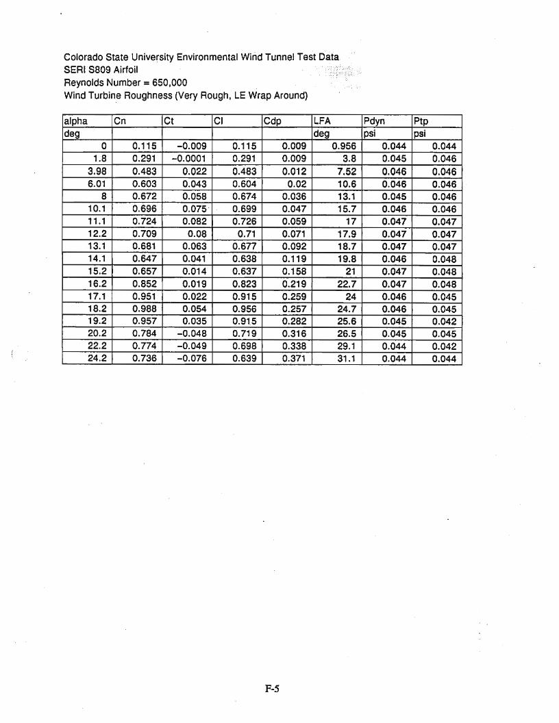
Colorado State University Environmental Wind Tunnel Test DataSERIS809 AirfoilReynolds Number = 650,000Wind Turbine Roughness (Very Rough, LE Wrap Around)
alpha Cn Ct CI Cdp · LFA Pdyn Ptpdeg deg psi psi
0 0.115 -0.009 0.115 0.009 0.956 0.044 0.0441.8 0.291 -0.0001 0.291 0.009 3.8 0.045 0.046
3.98 0.483 0.022 0.483 0.012 7.52 0.046 0.0466.01 0.603 0.043 0.604 0.02 10.6 0.046 0.046
8 0.672 0.058 0.674 0.036 13.1 0.045 0.04610.1 0.696 0.075 " 0.699 0.047 15.7 0.046 0.04611.1 0.724 0.082 0.726 0.059 17 0.047 0.04712.2 0.709 0.08 0.71 0.071 17.9 0.047 0.04713.1 0.681 0.063 0.6n 0.092 18.7 0.047 0.04714.1 0.647 0.041 0.638 0.119 19.8 0.046 0.04815.2 0.657 0.014 0.637 0.158 . 21 0.047 0.04816.2 0.852 0.019 0.823 0.219 22.7 0.047 0.04817.1 0.951 0.022 0.915 0.259 24 0.046 0.04518.2 0.988 0.054 0.956 0.257 24.7 0.046 0.04519.2 0.957 0.035 0.915 0.282 25.6 0.045 0.04220.2 0.784 -0.048 0.719 0.316 26.5 0.045 0.04522.2 ·0.774 -0.049 0.698 0.338 29.1 0.044 0.04224.2 0.736 -0.076 0.639 0.371 31.1 0.044 0.044
F-5
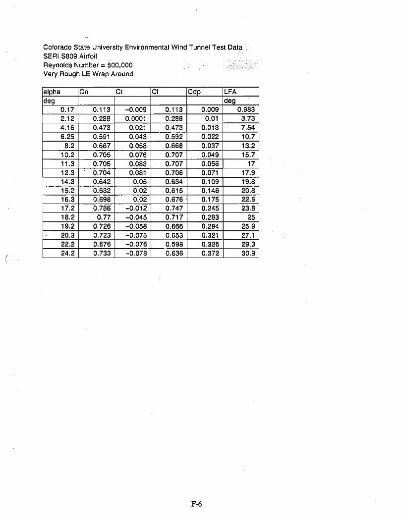
(
l
Colorado State University Environmental Wind Tunnel Test DataSERI S809 AirfoilReynolds Number =500,000Very Rough LE Wrap Around
alpha Cn Ct CI Cdp LFAdeg deg
0.17 0.113 -0.009 0.113 0.009 0.9832.12 0.288 0.0001 0.288 0.01 3.734.16 0.473 0.021 0.473 0.013 7.546.25 0.591 0.043 0.592 0.022 10.7
8.2 0.667 0.058 0.668 0.037 13.210.2 0.705 0.076 0.707 0.049 15.711.3 0.705 0.083 0.707 0.056 1712.3 0.704 0.081 0.706 0.071 17.914.3 0.642 0.05 0.634 0.109 19.815.2 0.632 0.02 0.615 0.146 20.816.3 0.698 0.02 0.676 0.175 22.517.2 0.786 -0.012 0.747 0.245 23.818.2 o.n -0.045 0.717 0.283 2519.2 0.726 -0.058 0.666 0.294 25.9
.s 20.3 0.723 -0.075 .0.653 0.321 27.122.2 0.676 -0.076 0.598 0.326 29.324.2 0.733 -0.078 0.636 0.372 30.9
F-6
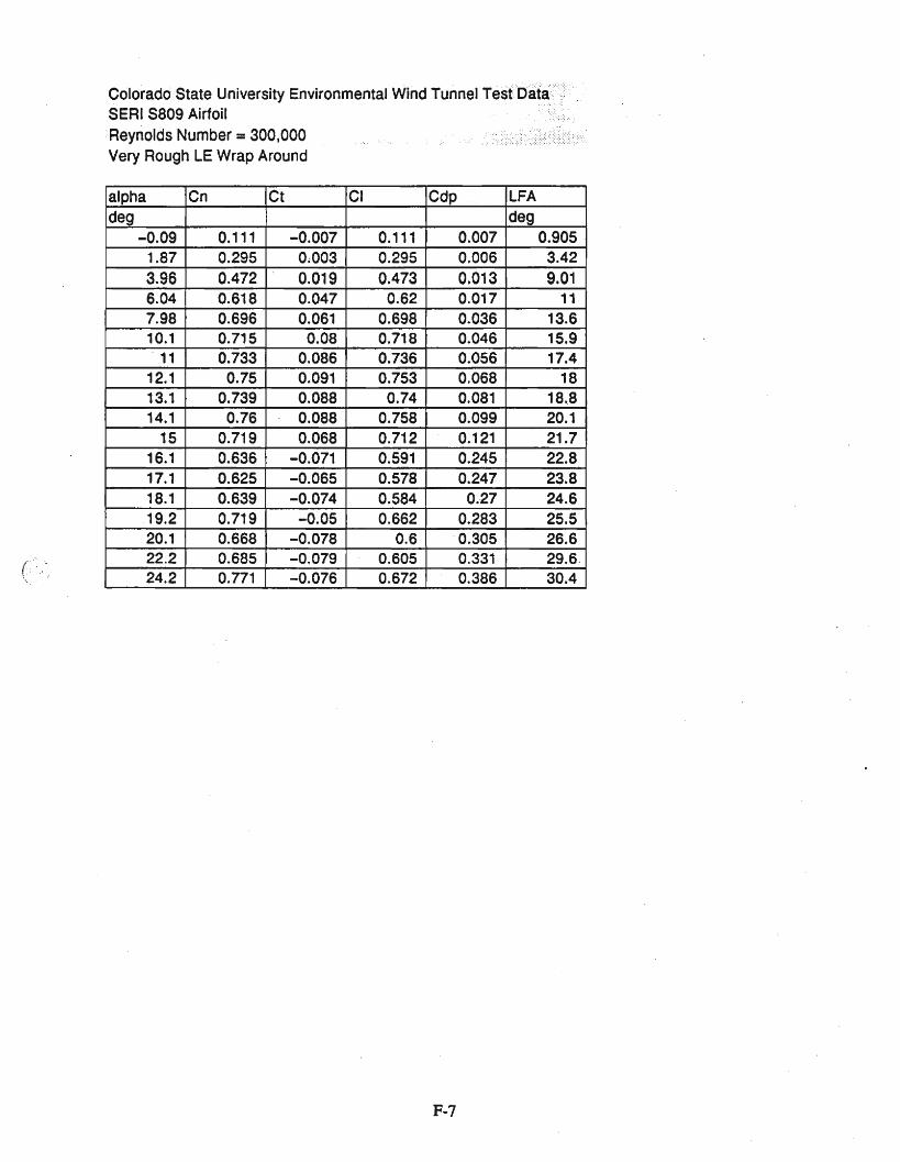
c.
Colorado State University Environmental Wind Tunnel Tesf6at~.~·· .: · . :SERI S809 Airfoil .:-t • . .
:Reynolds Number = 300,000 . ....Very Rough LE Wrap Around
alpha Cn Ct CI Cdp LFAdeg deg
-0.09 0.111 -0.007 0.111 0.007 0.9051.87 0.295 0~003 0.295 0.006 3.423.96 0.472 0.019 0.473 0.013 9.016.04 0.618 0.047 0.62 0.017 117.98 0.696 0.061 0.698 0.036 13.610.1 0.715 0.08 0.718 0.046 15.9. 11 0.733 0.086 0.736 0.056 17.4
12.1 0.75 0.091 0.753 0.068 1813.1 0.739 0.088 0.74 0.081 18.814.1 0.76 0.088 0.758 0.099 20.1
15 0.719 0.068 0.712 0.121 21.716.1 0.636 -0.071 0.591 0.245 22.817.1 0.625 -0.065 0.578 0.247 23.818.1 0.639 -0.074 0.584 0.27 24.619.2 0.719 -0~05 0.662 0.283 25.520.1 0.668 -0.078 0.6 ' 0.305 26.622.2 0.685 -0.079 0.605 0.331 29.6 .24.2 0.771 -0.076 0.672 0.386 30.4
F-7
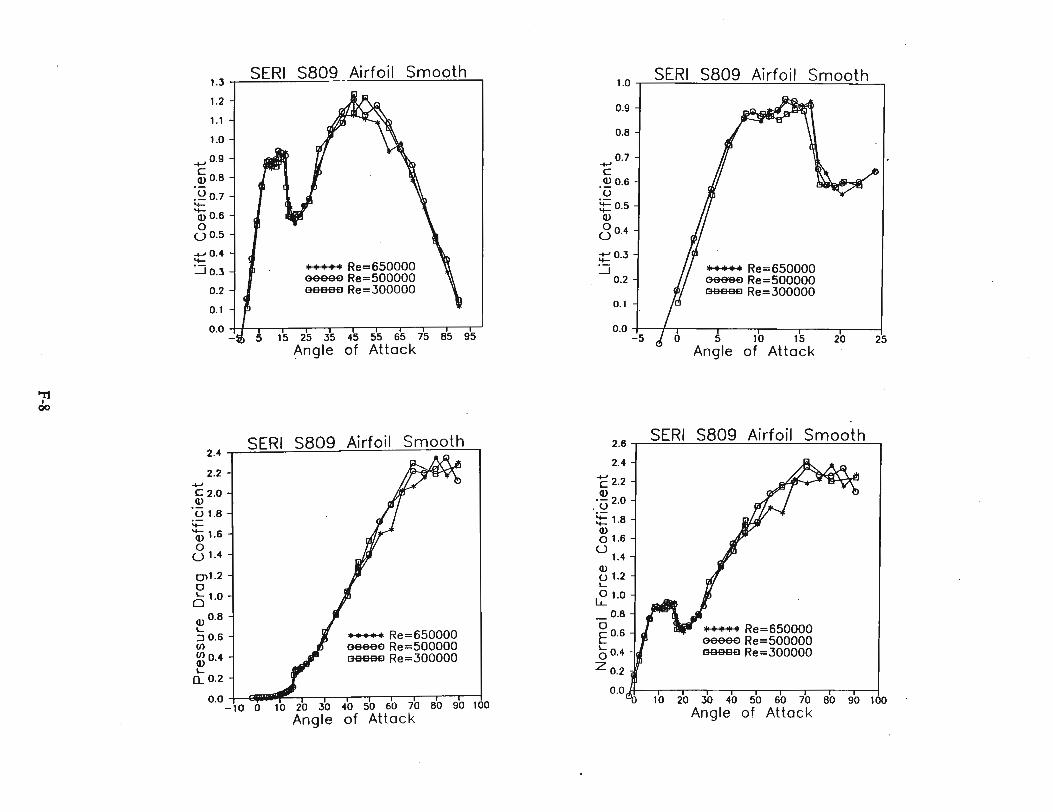
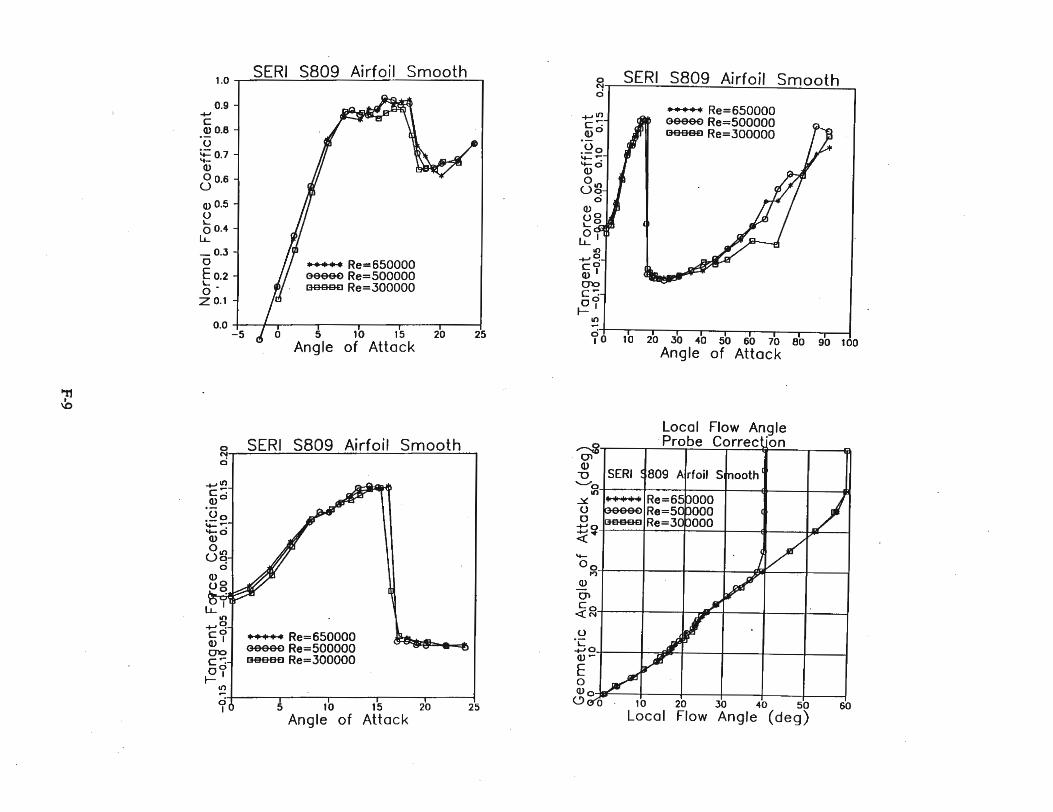

Appendix G
Pressure Distributions' forReynolds Number 650,000 Smooth
G-l


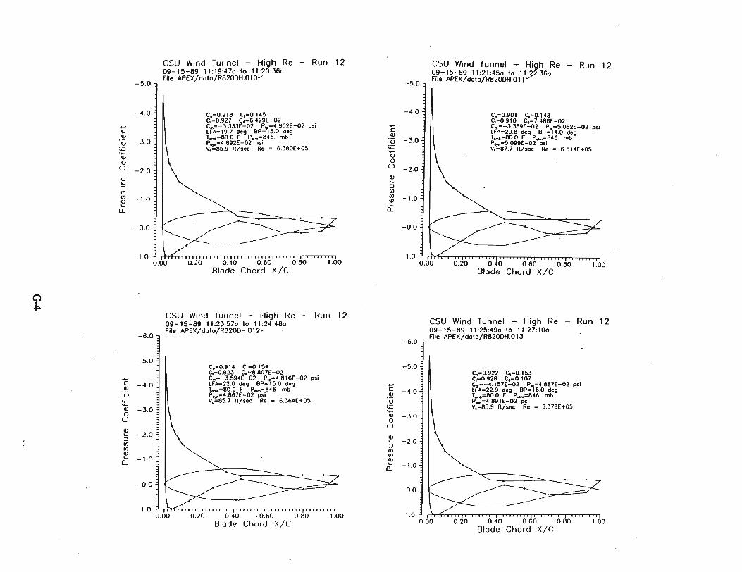

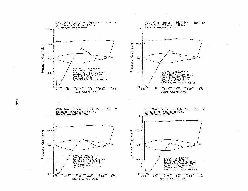
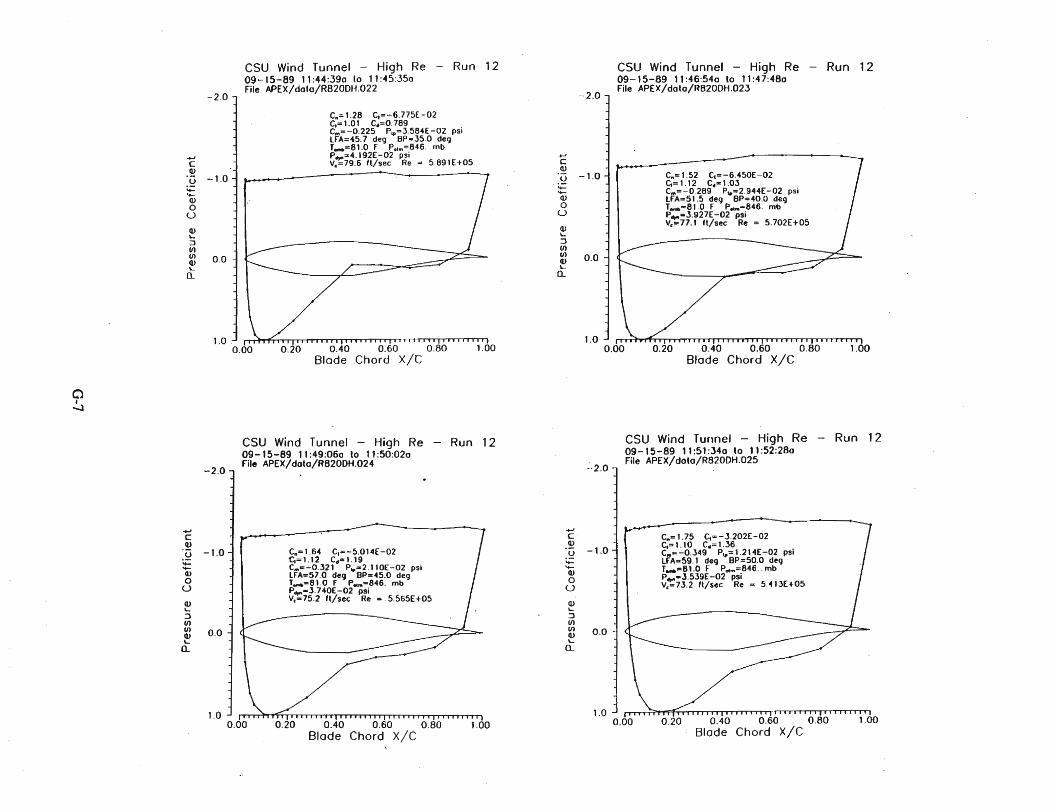

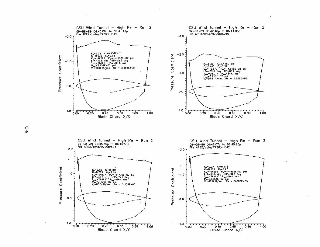
Appendix H
Pressure Distributions for Reynolds Number 650,000 Rough
H-l
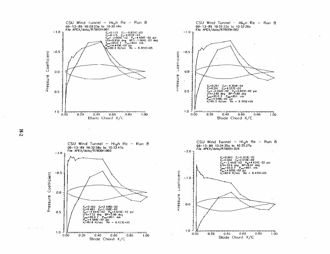

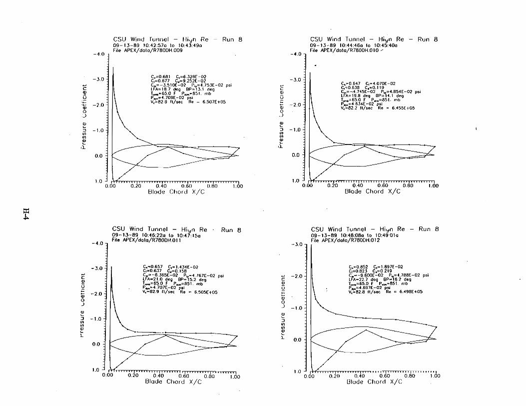
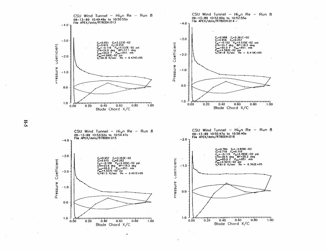
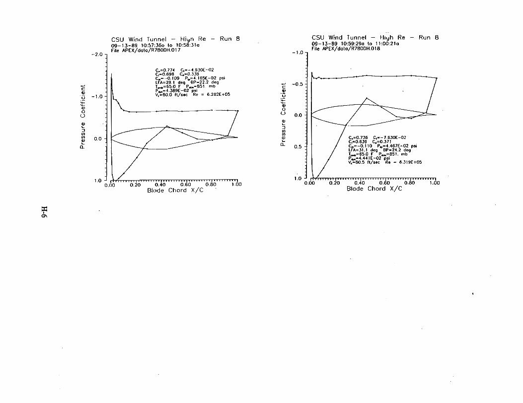

Appendix I
Pressure Distributions forReynolds Number 500,000 Smooth
1-1
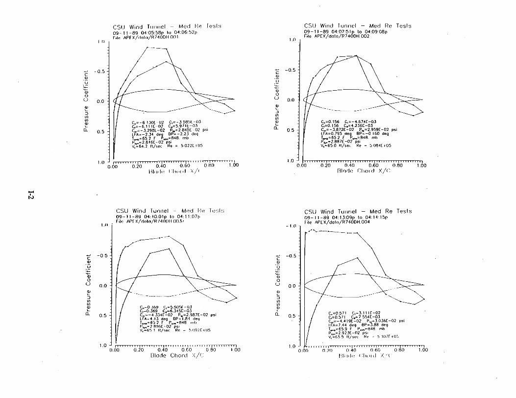

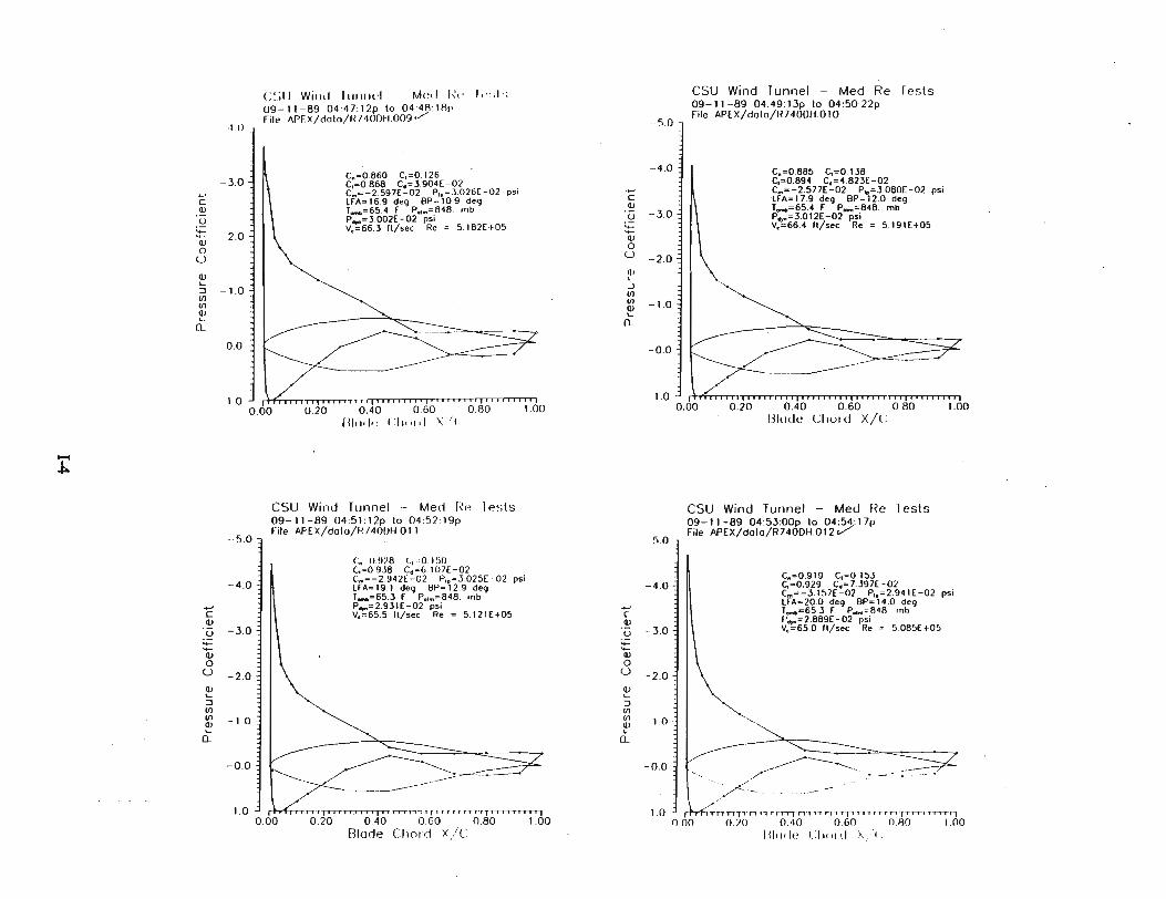
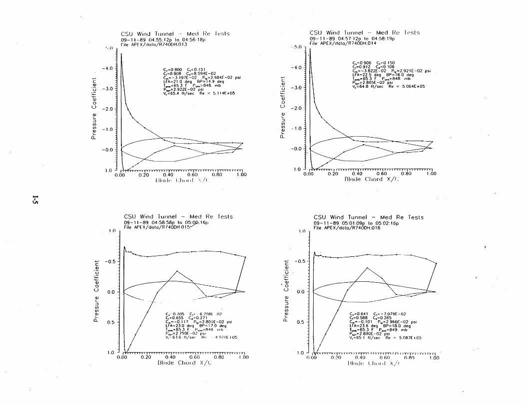
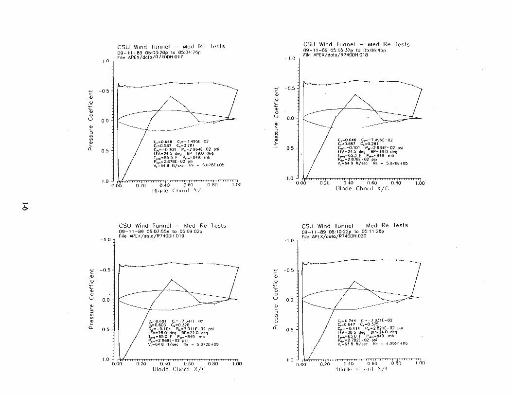


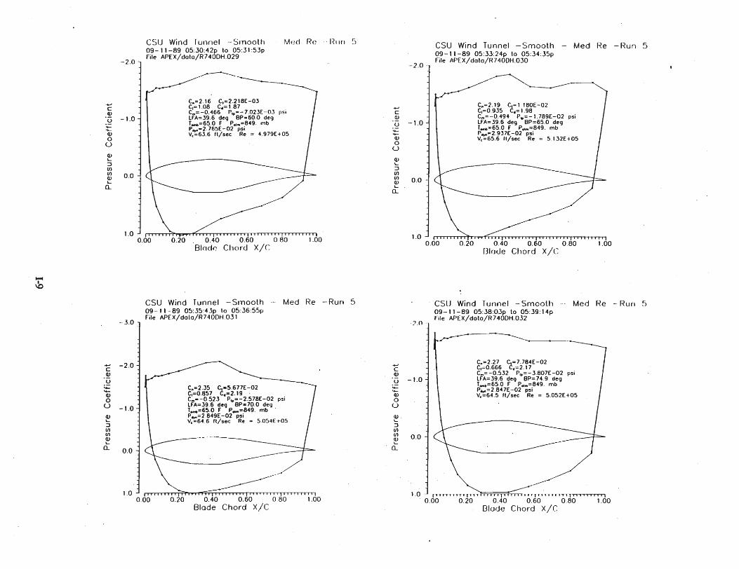


Appendix J
Pressure Distributions for Reynolds Number 500,000 Rough
J-l


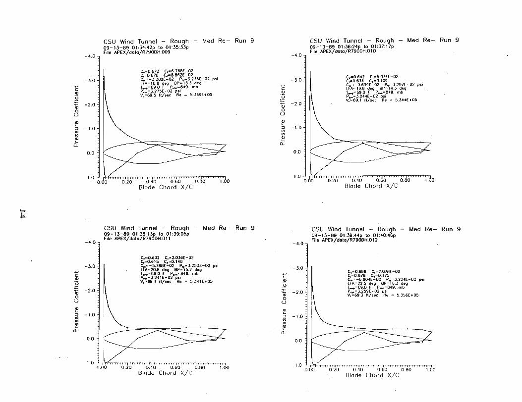


Appendix K
Pressure Distributions forReynolds Number 300,000 Smooth
K-l
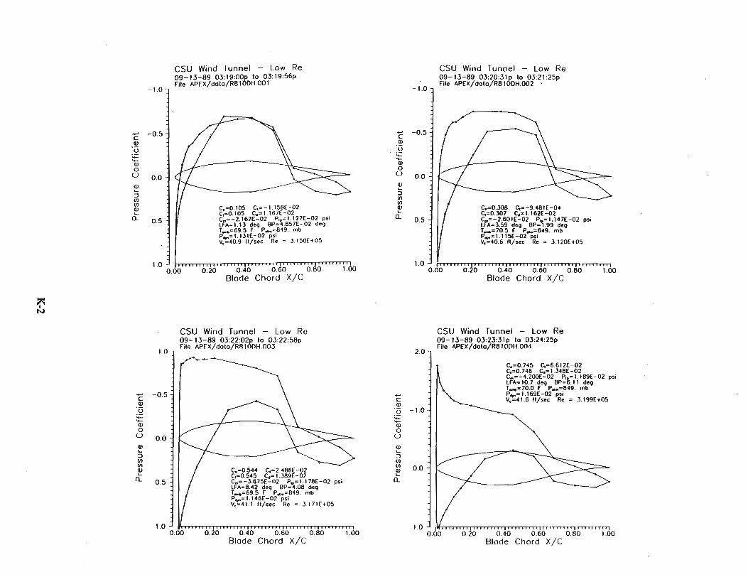
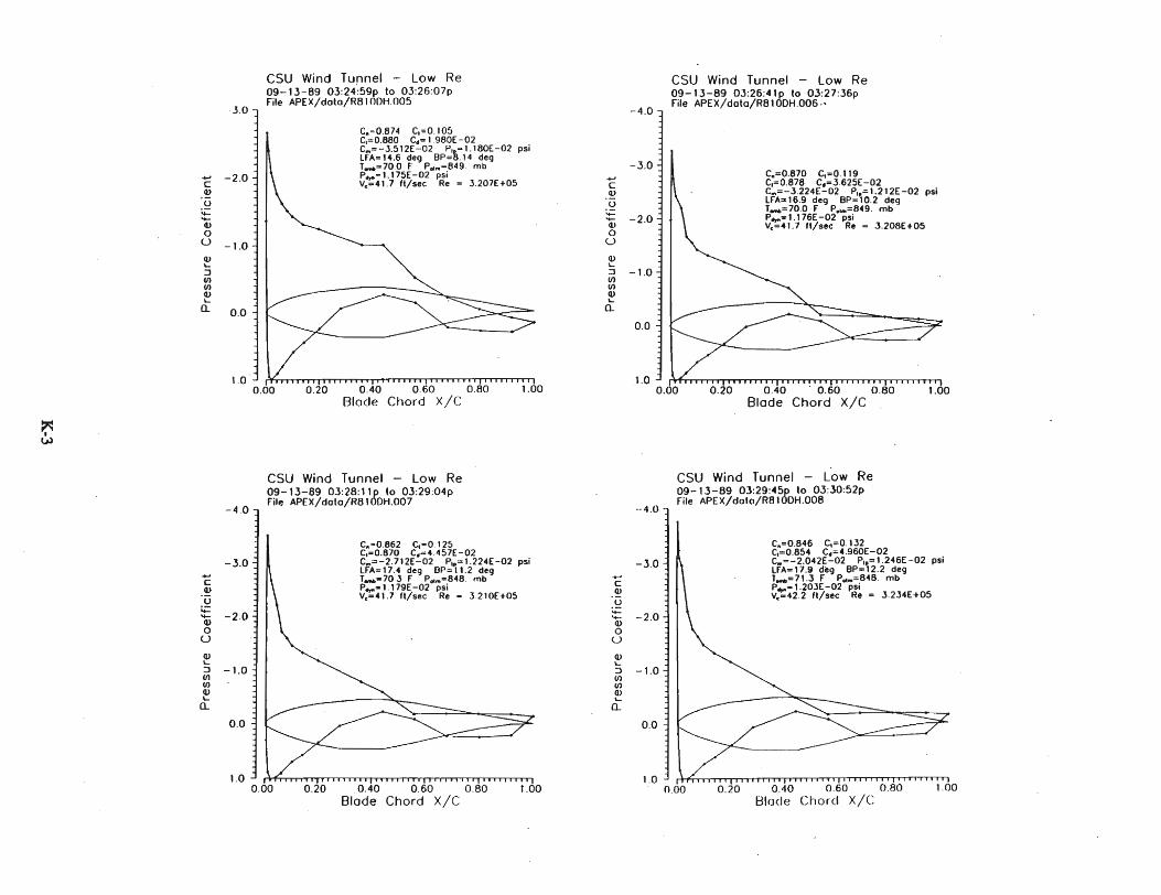


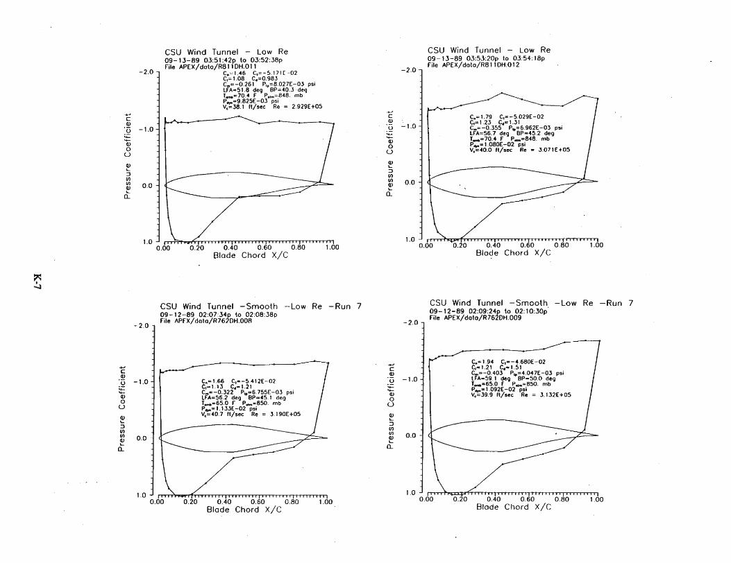
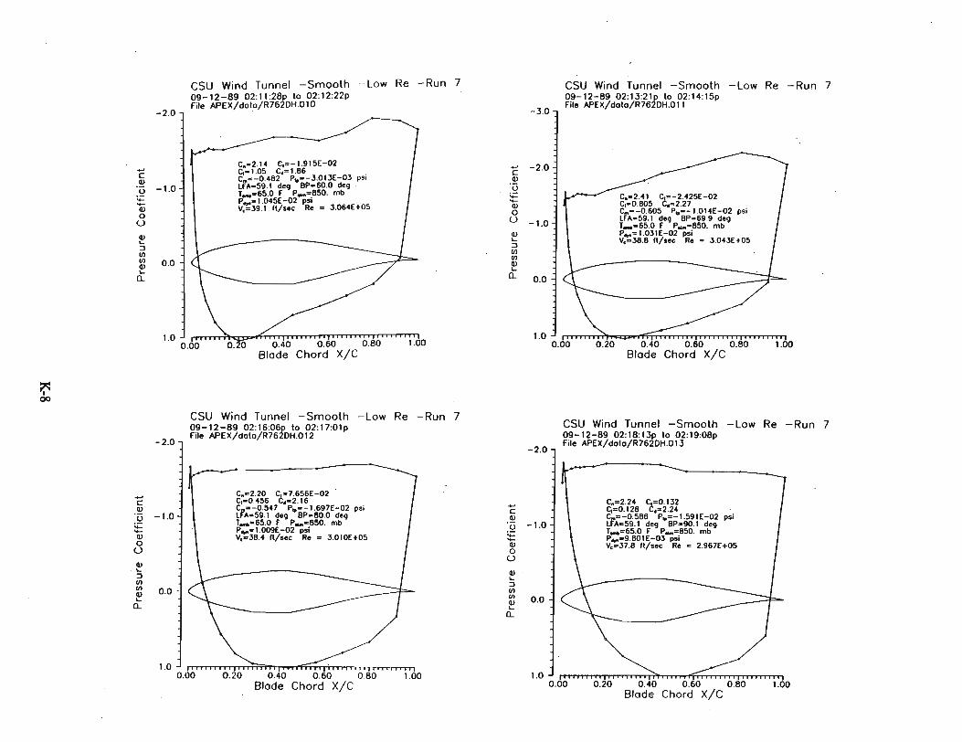

Appendix L
Pressure Distributions for Reynolds Number 300,000 Rough
L-l
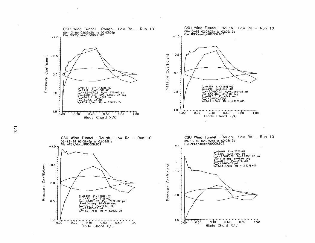


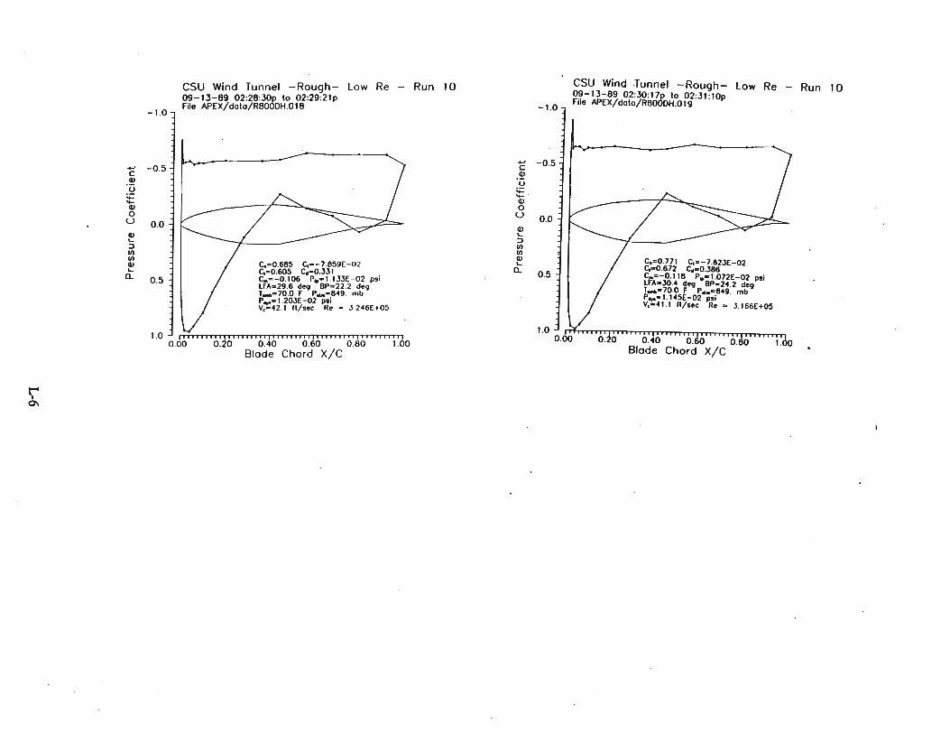

Document Control Page 1. NREL Report No.
NRElII'P·2S7-46S5
2. NTIS Accession No.
·0893000012
3. Recipienfs Accession No.
4. Title and Subtitle
Combined Experiment Phase I-Final Report
7. Author(s)C.P. Butterfield, W.P. Musial, D.A. Simms
9. Performing Organization Nameand Address
National Renewable Energy Laboratory1617 Cole Blvd.Golden. CO 80401
12. Sponsoring Organization Name and Address
NatiowRenewableEner~~
1617 Cole Blvd.Golden. CO 80401
15~ Supplementary Notes
16. Abstract (Umlt:200 words)
5. Publication DateOctober 1992
6.
8. Performing Organization Rept. No.
NREUI'P-2S7-4655
10. ProJecVTaskIWork Unit No.WE21.8101
11. Contract (0) or Grant (G) No.
(0)
(G)
13. Type of Report& PeriodCoveredTechnical Report
14.
How does wind tmmel airfoil data differ from the airfoil performance on an operating horizontal axis wind turbine (HAWf)?The National Renewable Energy laboratory has been conducting a comprehensive test program focused on answering thisquestion and understanding the basic fluid mechanics of rotating HAWf stall aerodynunics. The basic approach was toinstrument a wind turbine rotor, using an airfoil that was well documented by wind funnel tests, and measure operating pressuredistributions on the rotating blade. Based on the integrated values of the pressure data, airfoil perfonnance coefficients wereobtained, and comparisons were made between the rotating data and the wind tunnel data. Care was taken to minimize theaerodynamicand geometric differences between the rotating and the wind tunnel models
This is the first of two reports describing the Combined Experiment Program and its results. This Phase I report coversbackground information such as test setup and instrunlc'ntanon. It also includes wind tunnel test results androughness testing.
17. Document Analysis8. Desaiptors
wind turbines; wind turbine experimentalrotor dynamics; wind turbine aerodynamic pressure measurements
b. Identifiers/Open-Ended Terms
c. UOCategories261
18. Availability StatementNationalTechnical InfonnationServiceU.S. Department of Conunerce5285 PortRoyal RoadSpringfield, VA 22161
FormNo. 0069B (6-30-87)
19. No. of Pages
222
20. Price
A10