combining classification with fmri-derived complex network

Combining Classification with fMRI-Derived ComplexNetwork Measures for Potential NeurodiagnosticsTomer Fekete1., Meytal Wilf2., Denis Rubin1, Shimon Edelman3, Rafael Malach2, Lilianne R.

Mujica-Parodi1*

1 Department of Biomedical Engineering, State University of New York at Stony Brook, Stony Brook, New York, United States of America, 2 Department of Neurobiology,

Weizmann Institute of Science, Rehovot, Israel, 3 Department of Psychology, Cornell University, Ithaca, New York, United States of America

Abstract

Complex network analysis (CNA), a subset of graph theory, is an emerging approach to the analysis of functionalconnectivity in the brain, allowing quantitative assessment of network properties such as functional segregation,integration, resilience, and centrality. Here, we show how a classification framework complements complex network analysisby providing an efficient and objective means of selecting the best network model characterizing given functionalconnectivity data. We describe a novel kernel-sum learning approach, block diagonal optimization (BDopt), which can beapplied to CNA features to single out graph-theoretic characteristics and/or anatomical regions of interest underlyingdiscrimination, while mitigating problems of multiple comparisons. As a proof of concept for the method’s applicability tofuture neurodiagnostics, we apply BDopt classification to two resting state fMRI data sets: a trait (between-subjects)classification of patients with schizophrenia vs. controls, and a state (within-subjects) classification of wake vs. sleep,demonstrating powerful discriminant accuracy for the proposed framework.

Citation: Fekete T, Wilf M, Rubin D, Edelman S, Malach R, et al. (2013) Combining Classification with fMRI-Derived Complex Network Measures for PotentialNeurodiagnostics. PLoS ONE 8(5): e62867. doi:10.1371/journal.pone.0062867

Editor: Satoru Hayasaka, Wake Forest School of Medicine, United States of America

Received September 14, 2012; Accepted March 28, 2013; Published May 6, 2013

Copyright: � 2013 Fekete et al. This is an open-access article distributed under the terms of the Creative Commons Attribution License, which permitsunrestricted use, distribution, and reproduction in any medium, provided the original author and source are credited.

Funding: This research was supported by the Office of Naval Research, Grant #N000140410051 (LRMP) and the National Science Foundation, Grant #0954643(LRMP). The funders had no role in study design, data collection and analysis, decision to publish, or preparation of the manuscript.

Competing Interests: The authors have declared that no competing interests exist.

* E-mail: [email protected]

. These authors contributed equally to this work.

Introduction

Recent years have seen a growing interest in the analysis of

functional connectivity [1] data resulting from brain mapping

techniques such as fMRI. Complex network analysis (CNA), a

subset of graph theory that focuses on the topologically complex

networks often found in nature, has proved to be a powerful

approach to quantifying important features of functional connec-

tivity. These include general network properties such as its

functional segregation, integration, resilience, and centrality [2], as well as

quantifying the contribution of individual brain regions to the

network at large.

CNA is performed on graphs, which topologically represent a

matrix of functional connectivity. Functional connectivity can be

derived from cross-correlation in different frequency bands,

spectral coherence, or mutual information [3–10]. Normally,

graph representations are obtained after excluding negative and

auto-connections and are thresholded to retain only strongest

connections, sometimes to the point of binarization.

Network properties can be defined globally, describing the

structure of the entire network (e.g., assortativity coefficient [11],

closeness centrality [12], characteristic path length [13], clustering coefficient

[13], global efficiency [14], graph transitivity [15], local efficiency [14],

modularity [16], small-worldness [17]). Or, they can be defined locally,

on a per-node basis, so as to focus on neural regions of interest

(e.g., node betweenness centrality [12], node degree/strength, node

characteristic path length [13], node clustering coefficient [13] and node

global and local efficiency [14].

Compared to voxel-based analyses used in more standard brain

mapping, CNAs are theoretically parsimonious. However, in

practice, the number of actual choices involved in CNA, such as the

measure of connectivity, the connection threshold and frequency

band chosen for the analysis, and the combinatorics associated

with their optimization, could result in thousands of derived

measures (see Figure S1). Thus, while CNA has the advantage of

providing a large number of options by which functional

connectivity can be probed, the diversity comes at the cost of

having to find the ‘‘best’’ network model, with its concomitant

multiple comparisons problem.

We propose that a natural and appealing means for reaping the

full benefits of CNA is through combining complex network

analysis with a learning procedure that seeks to optimize

classification based on CNA features. By this we mean that the

range of possible network measures derived from a given data set

can be used as features for machine learning algorithms aiming at

classifying functional data according to different subject groups or

experimental conditions. The results of the procedure can then be

assessed for significance without the need for correction for

multiple comparisons. Moreover, as we describe below, feature

selection incorporated into the classifier constitutes a clear-cut,

readily interpretable, unbiased means of model selection.

Classification based on CNA measures holds appeal also for

several other reasons. First, complex network analysis has proved

PLOS ONE | www.plosone.org 1 May 2013 | Volume 8 | Issue 5 | e62867

to be sensitive in probing network features of psychiatric and

neurological disorders [18–23]. Thus, incorporating CNA into the

powerful framework of machine learning promises to be clinically

applicable. Second, multivariate classification methods make it

possible to explore how different measures of integration and

segregation interact in characterizing complex brain conditions,

including pathology.

Complex network measures can be naturally grouped into

families: all global measures (both binary and weighted) derived

from a single graph can be grouped together to what for

simplicity’s sake we will refer to as a graph. Similarly, local or

per-node measures computed across different graphs can be

grouped according to brain regions of interest, which we will refer

to as an ROI. We suggest that when applying machine learning to

complex network measures, feature selection should be carried out

by feature family; that is, by graph or ROI. In each case, model

selection can be based on the performance of the feature families

in question in supporting classification, that is, on discriminating

ability between subject groups or experimental conditions. Once

multivariate significance is established, the implicated ROIs/

graphs can be further probed through post hoc analysis, enabling

to focus on differences at a single-feature level to the degree they

are present in the data.

The scenario in which features are fed to a classifier by families

is commonly referred to as multiple kernel learning (MKL, [24]).

In what follows, we describe a complete MKL optimization

scheme incorporating graph/ROI selection: block diagonal

optimization (BDopt). As a proof of concept, we describe the

application of our scheme for complex network based classification

to two resting state fMRI data sets designed to elicit trait (between-

group; N = 18 patients with schizophrenia vs. controls) and state

(within-group; N = 10 wake vs. sleep) differences, and show how

CNA classification is not only useful in itself, but enables efficient

exploration of the organization of functional architectures under

various brain states.

Methods

In this study we analyzed two resting state fMRI data sets,

comparing schizophrenia patients vs. controls, as well as wake vs. sleep.

Detailed information on data collection in experiment 2 is

provided in Supplementary material S1. Formal definitions for

all graph theoretic terms are provided in Supplementary material

S2. This study was approved by the Institutional Review Board of

the Weizmann institute of science; all participants provided

informed written consent.

2.1 Data set 1– between-subjects Classification(Schizophrenic Patients vs. Controls)

2.1.1 Study design. Data were acquired from a publicly

available resting state fMRI dataset (http://hdl.handle.net/1926/1687). These data were collected and shared as per of the

National Alliance for Medical Image Computing (NA-MIC)

initiative, supported through the National Institutes of Health

Roadmap for Medical Research, Grant U54 EB005149. Subjects

were scanned using fMRI under resting state (closed-eyes)

conditions, and included 18 males, of which eight were patients.

There were no significant differences in age handedness or IQ

(WIS) between patients and controls (see Table 1). Patients were

medicated (all with atypical drugs, 1 with a conventional drug as

well).

2.1.2 Image acquisition. fMRI scans were acquired using a

3T GE scanner at Brigham and Women’s Hospital in Boston, MA,

using an echo planar imaging (EPI). An eight-channel coil was

used to perform parallel imaging using ASSET (GE) with a

SENSE-factor = 22. Runs were 10 minutes long, comprised 200

repetitions of a high resolution EPI scan (96696 in plane, 3 mm

thickness, TR-3000 ms, TE = 30, 39 slices).

2.1.3 Image analysis. Standard preprocessing procedures

were performed in SPM8 [25] including image realignment

correction for head movements, normalization to standard

26262 mm Montreal Neurological Institute space, and spatial

smoothing with a 6-mm full width at half maximum Gaussian

kernel. SPM movement estimates, as well as their squared

magnitudes were regressed out of fMRI time series, as were the

average time series from white matter, csf and global signal.

Finally, the time series were detrended. Data for one patient

exhibiting excessive movement were discarded.

2.2 Data set 2–Within-subjects Classification (Wake vs.Sleep)

2.2.1 Study design. Ten healthy volunteers (4 female, ages

25.662) participated in this study and were scanned under two

conditions: awake and asleep. For exact details see supplementary

material S1.

2.2.2 Image acquisition. The experiment was performed on

a Siemens 3 Tesla Trio Magnetom MRI scanner, with birdcage

radio frequency (RF) coil and a head only gradient coil designed

for EPI. Functional images of blood oxygenation level dependent

(BOLD) contrast comprising 46 axial slices were obtained with a

T2*-weighted gradient echo EPI sequence (TR = 3000 ms, TE

= 30, flip angle = 90u, FOV 240 mm, matrix size 80680, no gap

36363 mm voxel, ACPC) covering the whole brain.

2.2.3 Image analysis. Before analysis data were segmented

into 180 TR sequences that were scored for sleep. Segments

meeting the criteria for further analysis were preprocessed

separately. Preprocessing procedures were performed in SPM8,

including image realignment correction for head movements,

normalization to a 36363 mm Montreal Neurological Institute

template, and spatial smoothing with a 8-mm full width at half

maximum Gaussian kernel. The non-brain component of the time

series, assessed by averaging the signal in the ventricles, was

regressed out of fMRI time series [26], as were SPM movement

estimates, and after which time series were detrended. Following

the recommendation of a previous CNA study of sleep fMRI [27]

we avoided regressing out the global signal in this case. Segments

exhibiting excessive movement (.1 mm) were discarded. This

resulted in 44 segments total (21 sleep), such that there was at least

one example from each condition per subject.

2.3 Deriving Graphs from Imaging DataThe connectivity metrics chosen for this study were the

correlation and partial correlation coefficients. We first extracted

the average time series from the 116 automated anatomical

labeling ROIs [28], which span the brain gray matter, using WFU

Table 1. Demographics of participants in study 1(Schizophrenic Patients vs. Controls).

age handedness IQ (WIS)

Patients 44.1611.4 0.7860.18 102.4620.9

Controls 41.8611.2 0.7360.28 117.5617.4

Significance 0.67 0.28 0.12594

Significance was assessed using two sided two sample t-tests.doi:10.1371/journal.pone.0062867.t001

Complex Network Based Classification


pickAtlas [29]. The resulting time series were filtered into the

0.01–0.1 Hz [22] and 0.03–0.06 Hz frequency bands [30]. For

each time series array - both the filtered and original time series -

we computed the lagged correlations and partial correlations

ranging from 63TR and also derived the maximal correlation of

the seven. Negative values were set to zero, as well as

autocorrelations. The correlation matrices were thresholded to

leave a fraction a of the strongest connections using

a~ :5 :4 � � � :1½ � to produce 240 graphs (3626865; fre-

quency bands, linear/partial correlation, seven lags and their

maximum and five thresholds respectively - see Figure S1). From

each resulting connectivity matrix both weighted and binary

global features were harvested. For local measures, we focused on

a subset of these graphs that has been reported to be

discriminative, zero lagged partial correlations in the 0.01–

0.1 Hz band [22], from which both binary and weighted features

were derived for each ROI.

2.4 Complex Network MeasuresThe global measures employed in this study were: assortativity

coefficient [11], closeness centrality [12], characteristic path length [13],

clustering coefficient [13], global efficiency [14], graph transitivity [15], local

efficiency [14], modularity [16], small-world ratio. The local measures

[22] we utilized were: node betweenness centrality [12], node degree/

strength (the sum of edges), node characteristic path length [13], node clustering

coefficient [13], and node global and local efficiency [14].

The reason we chose to use the small world ratio rather than

small world index is twofold: for the binary ratio, normalization by

the random small world ratio is vestigial - it is a mere

multiplication by a constant that is factored out when features

are normalized for scale before classification. In the weighted case,

due to the exponentially greater combinatorial complexity, ratio

estimates are associated with random variance introduced solely

by permutation analysis, a clear artifact. We therefore applied

normalization only during post-hoc analysis.

2.5 Motion AnalysisTo compare head motion between groups five metrics were

computed for each data point using the motion estimates resulting

from SPM8’s correction procedure. These metrics were later

compared between groups using a t-test: 1) maximal displacement

across xyz coordinates, 2) maximal degree shift 3) average

translation 4) average rotation 5) frame displacement [31].

2.6 ClassificationThe goal of a classifier is to label data in a test set (e.g., patient

vs. control, sleep vs. wake) according to information gleaned from

learning data. All classification reported here was done using our

NeuroClass (http://www.lcneuro.org/) - a publicly available

Matlab toolbox for SVM based classification. NeuroClass utilizes

the LIB-SVM toolbox [32] as its computational core.

2.6.1 Feature scaling. Prior to analysis, each feature was

normalized across subjects in the training sample via a z transform

and the estimated mean and standard deviation were used to scale

the test data. Normalization is required to avoid driving results due

to trivial scale differences between features, and the necessity to

adapt classifier parameters to scale.

2.6.2 Multi kernel Block Diagonal optimization

(BDopt). Applying complex network analysis to neuroimaging

data results in various features (i.e., measures), which in turn could

simply be fed into a classifier. However, there are two substantial

reasons for treating complex network measures as families of

features rather than individual features. In the case of global

measures, it is natural to treat various measures originating from a

single graph as a single multidimensional representation, as

different measures afford complementary information regarding

basic properties of the dynamics: segregation, integration, central-

ity and resilience of the network [2]. In the case of local measures,

grouping features according to ROI enables one to characterize a

brain region in terms of its significance to the network as a whole,

as well as to anatomically localize group differences in the case of

pathology.

A general family of learning machines in which this can be

naturally implemented is kernel sum machines, which is referred

to as multiple kernel learning [MKL, 24]. In MKL, each family of

features is used to derive a kernel matrix: (xri ,x

rj ).kr

ij where xri is

the feature vector originating from the rth anatomical region (or

graph) derived from the ith observation. Next, the kernels derived

from all feature families are summed to produce a single kernel K,

i.e.: K~PR

r~1

wrKr. This kernel can then be fed to a kernel based

learning machine such as a support vector machine (SVM).

We developed a novel optimization method for deriving optimal

weights for feature families: multi kernel block diagonal optimi-

zation (BDopt). The kernel matrix can be thought of as

representing the degree of similarity between feature vectors. In

BDopt, the optimal weight vector w is found by maximizing the

ratio of within-class to between-class similarity. In the ideal

scenario – which would lead to perfect classification – the

similarity within class would be maximal, e.g., attain some

maximal value s for each pair of observations belonging to the

group, while the similarity between instances belonging to different

groups would be virtually zero. If the data are organized according

to class, that is, first the examples belonging to the first class,

followed by the examples from the second class and so on, then the

resulting kernel matrix would have the form of a block diagonal

matrix: the matrix entries corresponding to within class similarity

would attain the value s, while all other values would be

zero.(Figure 1). In general, this ideal similarity structure can be

represented by a block-diagonal binary matrix. Thus wr can be

found by minimizing the quadratic difference between the

weighted sum of kernels and the block diagonal matrix B, i.e.:

arg minw

PR

r~1

wrKr{B

��

��

2

. This is, in fact, an ordinary least

squares regression problem whose solution is given by

wopt~~kkT (~kkT~kk){1~bb, where ~kkT and ~bb respectively denote the

(column) vector representations of K and B. In the analysis

described here, we applied BDopt to our data using a spherical

kernel, i.e.: Krij~

xri

xrik k: xr

j

xrjk k

. The resulting SVM needs to be

optimized for the soft margin parameter C to achieve optimal

results as is always the case with SVM classification.

2.6.3 Feature selection. In high dimensional classification,

feature selection is crucial because increasing the dimensionality

(number of features) leads to accumulation of not only signal, but

also noise. Therefore, it is quite likely that for noisy features, the

information they carry might be masked by noise as the number of

features becomes excessive [33]. This is true both for the number

of feature families (ROIs, graphs), and for the dimensionality of

each family. BDopt readily allows for feature selection at both

levels.

To select features within each family, we used the squared two-

sample t-statistic [33], which allows the features to be ranked

according to their discriminative power, given the training sample.

After the features were ranked, only the top k% of the features in

each family was retained. Note that this extends to multiclass



scenarios in which the F statistic resulting from an ANOVA can be

used.

To select feature families, recursive feature elimination (RFE,

[34]), can be applied to the weighted kernels (i.e., RCK; [35]). In

each iteration, an SVM is trained on the training sample, and the

resulting weights are used to find the feature family that

contributes the least to the classification. The quadratic norm of

the SVM weights is given by wSVMk k2~aT Ka~aT (

Pr wrK

r)a.

Given that the contribution of each weighted kernel to the SVM

weights is aT wrKra, the least informative feature family is

determined by arg minr

aT wrKra. This feature family can then

be removed, and the process repeated. Note that this optimization

results in a ranking of feature families according to their

discriminative power.

2.6.4 Cross-validation. Due to the small number of subjects

in typical human neuroimaging studies, the most suitable choice

for cross-validation (CV) seems to be a leave one out (LOO)

scheme. In LOO, each subject in turn is removed from the pool.

Next, classification is carried out on the remaining subjects

(training data). Finally, the model is tested on the withheld subject

(test) data, after which the test data is returned to the pool. The

result for all subjects is averaged to yield a success rate.

In classification of neuroimaging time series, the dimensionality

(number of features) greatly exceeds the number of data points,

which can lead to overfitting the data. Overfitting can be

circumvented by taking several measures. First, it is critical to

carry out feature selection in conjunction with cross validation, i.e.,

independently for each training sample (the data after removing

example i), otherwise the classification results will be biased,

resulting in an inflated success rate. Second, regardless of the

choice of kernel, SVMs have at least one hyper-parameter that has

to be optimized for. Therefore, an additional CV step is necessary

to find both the optimal number of feature families (i.e., ROIs or

graphs) and the optimal SVM parameters. This means that for

each of the LOO training sets, an additional LOO CV is carried

out to select the abovementioned parameters. After they are

computed, the model can be retrained on the full LOO training

set, and tested on the withheld data. Given the small number of

samples in a typical neuroimaging classification scenario, it is

common for several parameter combinations to yield the maximal

success rate, making the choice of a specific optimal combination

of parameters arbitrary. We must, therefore, retain multiple

versions of the trained classifier, corresponding to the multiple

optimal combinations of parameters, and let the test outcomes be

decided by a majority vote among those.

BDopt, and all the associated methods described herein were

developed and tested on an independent data set of N = 33

schizophrenia patients and controls that we had previously

collected [36]. Those data suggested that in general the spherical

kernel appears to be a reasonable choice for classification, as it

strikes a balance between nonlinear kernels, which have more

parameters and are therefore more prone to overfitting, and the

more robust but less discriminating linear kernel. BDopt

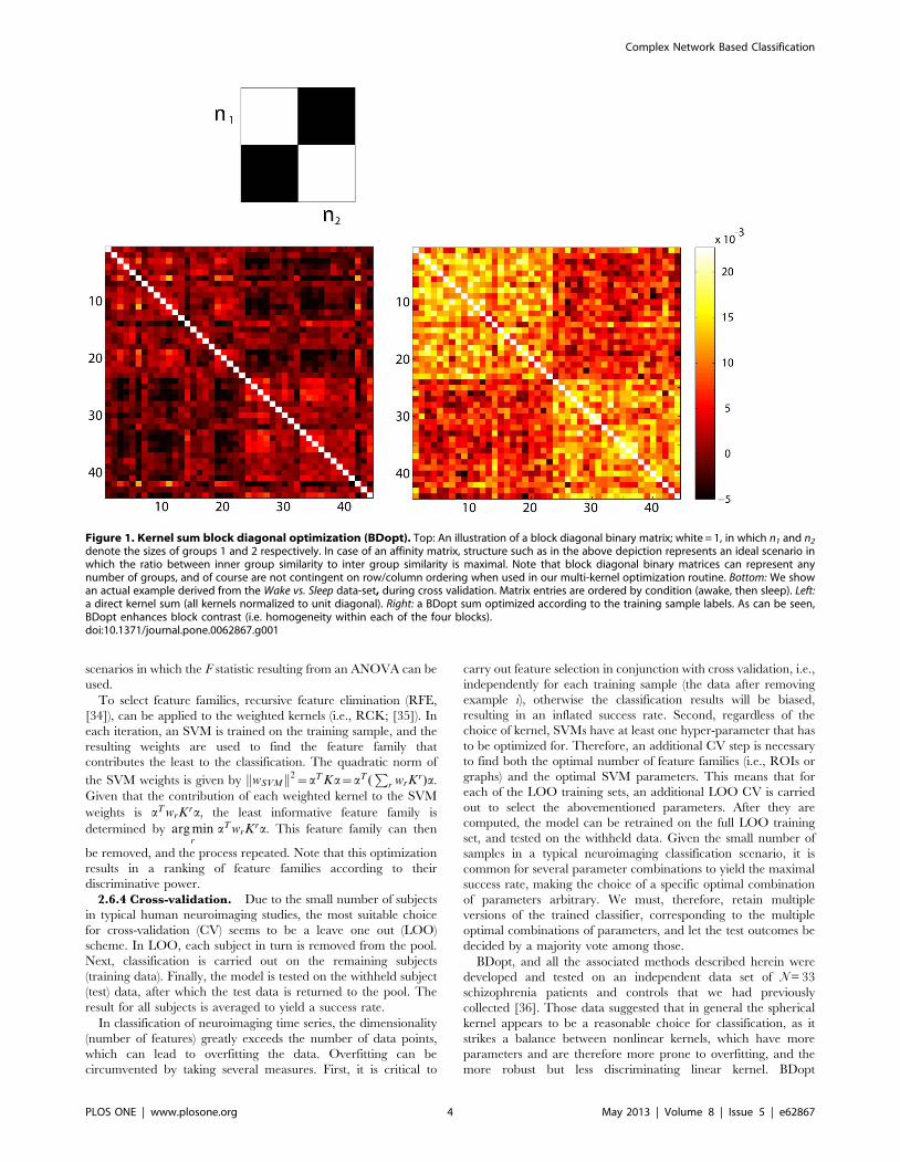
Figure 1. Kernel sum block diagonal optimization (BDopt). Top: An illustration of a block diagonal binary matrix; white = 1, in which n1 and n2

denote the sizes of groups 1 and 2 respectively. In case of an affinity matrix, structure such as in the above depiction represents an ideal scenario inwhich the ratio between inner group similarity to inter group similarity is maximal. Note that block diagonal binary matrices can represent anynumber of groups, and of course are not contingent on row/column ordering when used in our multi-kernel optimization routine. Bottom: We showan actual example derived from the Wake vs. Sleep data-set, during cross validation. Matrix entries are ordered by condition (awake, then sleep). Left:a direct kernel sum (all kernels normalized to unit diagonal). Right: a BDopt sum optimized according to the training sample labels. As can be seen,BDopt enhances block contrast (i.e. homogeneity within each of the four blocks).doi:10.1371/journal.pone.0062867.g001



classification as utilized in the present study is illustrated in Figure

S2.

2.6.5 Analysis of significance. Classification involving k

pattern classes applied to a test set results in a contingency table

(confusion matrix), that is, the frequency distribution NtestM(Ntest11,

Ntest12, …, Ntest

kk) of the patterns, where Ntestij denotes the number of

elements, belonging to class i, which were labeled by the classifier

as members of class j. Three methods have been commonly used to

assess the significance of such contingency tables [37]: Fisher’s

exact probability test [38], the x2 test (which is a poor

approximation when the sample size is small and contingency

cells may have low counts), and Monte Carlo methods. While

bootstrap methods are very appealing in this regard, due to the

computational intensity of RCK they are not feasible. According-

ly, in the analysis we describe below we deployed the exact

method.

2.6.6 Post hoc analysis. If the performance of a classifier has

proven to be significantly above chance, post hoc analysis can

indicate which are the graph measures driving the result. On

average (across CV folds), the performance of a classifier will peak

at a certain number of feature families. Thus application of BDopt

results in a unique subset of ranked graphs and ROIs. The CNA

can be further probed by paired t-tests on individual measures, to

assess the contribution of individual measures to the result.

If the number of contributing graphs or ROIs is substantial, it is

possible to carry out post hoc analysis on measure families, rather

than specific measures (e.g., the characteristic path length across

different graphs and ROIs). One approach would be to analyze

the distribution of the group comparison results for a given

measure for the ROIs implicated by the classifier. Feature families

that exhibited a higher fraction of significant comparisons than

expected by chance are sought after. Under the null hypothesis, a

single comparison is considered a random event generated by a

binomial distribution with a parameter of 0.05. Thus n events (e.g.

the comparisons across ROIs for a given measure) are can be

assessed for significance with B(n,0.05). Additionally, the resulting

p value is corrected for the number of features families. Further

still, for each feature family, the fraction of significant pairwise

comparisons for which the sign of the difference between groups

was consistent can be calculated serving as a measure of the

robustness of the result of the abovementioned analysis, and

assessed for significance utilizing a binomial distribution with a

parameter of 0.5, B(n,0.5). The resulting p-value is then corrected

for the number of feature families. Thus, feature families that

prove significant on both counts support group differences under a

given network measure.

Results

Both data sets were mined for global and local complex network

measures. The CNA measures were then used as classification

features. We compared the performance of several models - block

diagonal optimization (BDopt), recursive composite kernels (RCK;

[35]), recursive feature elimination (RFE, [34]), and standard

SVM classification - on both global and local CNA features. As a

control, classifier accuracy was compared to classification of the

functional connectivity pattern used to derive local features -

partial correlation in the 0.01–0.1 Hz frequency band - using

BDopt. In all cases the spherical kernel model was applied and

optimized for the soft margin parameter C = (221–26), and initial

feature selection, was according to a t2 threshold of 25%. All

classification experiments were carried out using NeuroClass

(http://www.lcneuro.org/) - a matlab toolbox for SVM based

classification. To rule out confounds to the results caused by

movement, we carried out two sample t-tests comparing maximal

displacement in coordinate and angle, average translation and

rotation, and frame displacement [31] between groups. No

significant differences were found for either of the five metrics in

both data sets: p = 0.29, 0.37, 0.41, 0.61,0.54, df = 43 for sleep vs.

wake and p = 0.20, 0.28, 0.11, 0.098, 0.11, df = 16 for

schizophrenia vs. control.

3.1 Data Set 1 (Patients with Schizophrenia vs. Controls)The results of the first classification experiment (patients vs.

controls) using global CNA features are shown in Table 2. BDopt

performed best achieving a success rate of 100%; Fisher’s exact

probability test confirmed the results to be significant

(p = 0.00005). Success rate was higher than achieved by RCK

and RFE, which both achieved 94% accuracy. In comparison,

application of SVM with the same parameters did not yield

significant classification.

The average minimal number of graphs necessary to achieve

perfect classification was 12. Table 3 lists the top twelve graphs

implicated by BDopt. We show a graphical representation of the

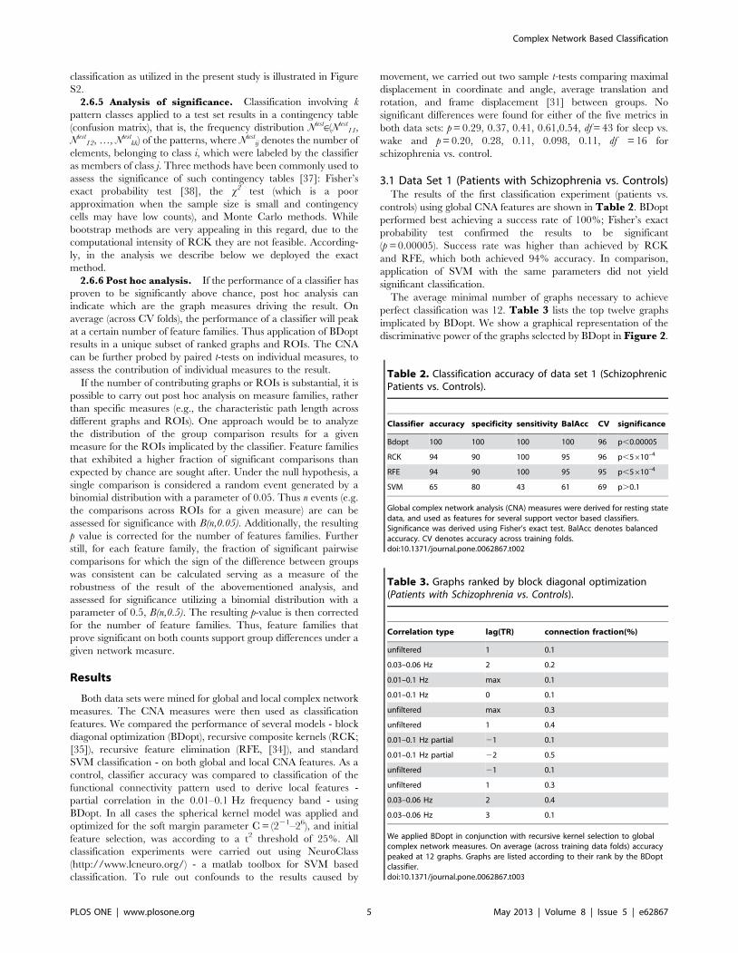
discriminative power of the graphs selected by BDopt in Figure 2.

Table 2. Classification accuracy of data set 1 (SchizophrenicPatients vs. Controls).

Classifier accuracy specificity sensitivity BalAcc CV significance

Bdopt 100 100 100 100 96 p,0.00005

RCK 94 90 100 95 96 p,5610–4

RFE 94 90 100 95 95 p,5610–4

SVM 65 80 43 61 69 p.0.1

Global complex network analysis (CNA) measures were derived for resting statedata, and used as features for several support vector based classifiers.Significance was derived using Fisher’s exact test. BalAcc denotes balancedaccuracy. CV denotes accuracy across training folds.doi:10.1371/journal.pone.0062867.t002

Table 3. Graphs ranked by block diagonal optimization(Patients with Schizophrenia vs. Controls).

Correlation type lag(TR) connection fraction(%)

unfiltered 1 0.1

0.03–0.06 Hz 2 0.2

0.01–0.1 Hz max 0.1

0.01–0.1 Hz 0 0.1

unfiltered max 0.3

unfiltered 1 0.4

0.01–0.1 Hz partial 21 0.1

0.01–0.1 Hz partial 22 0.5

unfiltered 21 0.1

unfiltered 1 0.3

0.03–0.06 Hz 2 0.4

0.03–0.06 Hz 3 0.1

We applied BDopt in conjunction with recursive kernel selection to globalcomplex network measures. On average (across training data folds) accuracypeaked at 12 graphs. Graphs are listed according to their rank by the BDoptclassifier.doi:10.1371/journal.pone.0062867.t003



Post hoc analysis could then be carried out on the individual

measures across groups, by applying two-sample t-tests. In general,

individual comparisons were moderately significant, and would

not have survived correction for multiple comparisons. However,

out of 216 (12 graphs618 features) comparisons, 55 were

significant (p,10–23 under a binomial test). Especially notable

was the binary small world ratio that was significant in 6 out of the

12 graphs. As can be expected in schizophrenia fMRI [18–21,39],

in all cases patients exhibited a smaller ratio, indicating

compromised efficiency of network topology (Table 4). The

difference between patients and controls in the small world index

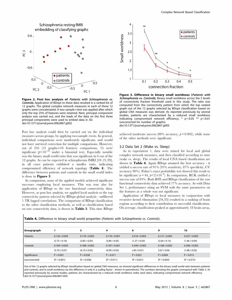
is show in Figure 3.

In comparison, none of the applied models achieved significant

successes employing local measures. This was true also for

application of BDopt to the raw functional connectivity data.

However, as post hoc analysis, we applied local analysis to the top

connectivity pattern selected by BDopt global analysis - unfiltered

1 TR lagged correlations. The comparison of BDopt classification

to the other classification methods, as well as classification based

on raw connectivity data, is shown in Table 5. This time BDopt

achieved moderate success (88% accuracy, p = 0.002), while none

of the other methods were significant.

3.2 Data Set 2 (Wake vs. Sleep)As in experiment 1, data were mined for local and global

complex network measures, and then classified according to state

(wake vs. sleep). The results of local CNA based classification are

shown in Table 6. Again BDopt attained the best accuracy - it

yielded a success rate of 91% (95% sensitivity, 87% specificity, CV

accuracy 90%). Fisher’s exact probability test showed this result to

be significant (n = 44, p,2610–8). In comparison, RCK yielded a

success rate of 84%. Both RFE and BDopt classification of the raw

functional connectivity data achieved 77% accuracy. As with Data

Set 1, performance using an SVM with the same parameters on

the features as a whole was not significant.

Application of BDopt to local measures in conjunction with

recursive kernel elimination [34,35] resulted in a ranking of brain

regions according to their contribution to successful classification.

On average, classification peaked at approximately 18 brain areas,

Figure 2. Post hoc analysis of Patients with Schizophrenia vs.Controls. Application of BDopt to these data resulted in a ranked list of12 graphs. The global complex network measures in each of these 12graphs were concatenated. A two sample t-test was applied after whichonly the top 25% of features were retained. Next, principal componentanalysis was carried out, and the loads of the data on the first threeprincipal components were used to embed data in 3D.doi:10.1371/journal.pone.0062867.g002

Table 4. Difference in binary small world properties (Patients with Schizophrenia vs. Controls).

Group/graph 1 3 4 6 9 10

Patients 0.12660.003 0.17660.002 0.17660.001 0.31660.003 0.12160.003 0.25760.003

(2.7560.10) (3.8560.05) (3.8460.05) (1.2760.03) (2.6460.15) (1.4660.04)

Controls 0.16960.003 0.18860.002 0.18760.001 0.34960.003 0.16860.003 0.29660.003

(3.7060.07) (4.1060.05) (4.0960.03) (.4060.01) 3.6760.06 (1.6860.02)

Significance P = 0.001 P = 0.038 P = 0.011 P = 0.021 P = 0.004 P = 0.015

[uncorrected] (P = 0.001) (P = 0.038) (P = 0.011) (P = 0.021) (P = 0.004) (P = 0.015)

Out of the 12 graphs selected by BDopt classification based on global CNA measures, six showed significant differences in the binary small world ratio between patientsand controls, and in small worldness (as the difference is only in a scaling factor - shown in parenthesis). The numbers denoting the graphs correspond with Table 3. Asreported previously by several studies, patients are characterized by a reduced small worldness index (and ratio), indicating compromised network efficiency.doi:10.1371/journal.pone.0062867.t004

Figure 3. Difference in binary small worldness (Patients withSchizophrenia vs. Controls). Binary small worldness across the 5 levelsof connectivity fraction threshold used in this study. The ratio wascomputed from the connectivity pattern from which the top rankedgraph out of the 12 graphs selected by BDopt classification based onglobal CNA measures was derived. As reported previously by severalstudies, patients are characterized by a reduced small worldnessindicating compromised network efficiency. * p,0.05 ** p,0.01(uncorrected for number of graphs).doi:10.1371/journal.pone.0062867.g003



which are shown in Table 7. In Figure 4, we show a graphical

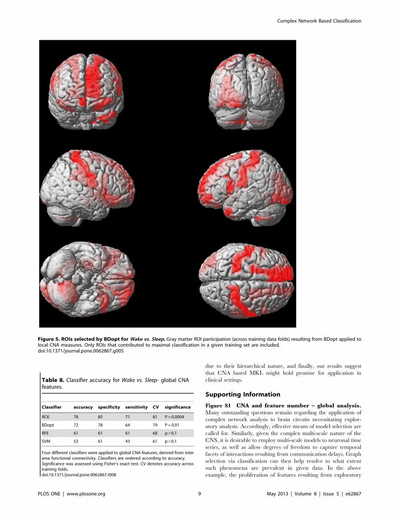
representation of these regions’ discriminative power. Figure 5highlights the implicated ROIs according to their participation

(the fraction of training data folds in which they were ranked

among the first 18 regions).

We then conducted post hoc analyses on the ranked ROIs, in

the form of paired t-tests for each measure/ROI conjunction

across groups. In general, as in the analysis of our first data set, p

values tended to be modest, and hence would not have survived

correction for multiple comparisons for number of regions, let

alone for the number of measures, models, and graphs tested.

However, out of 1080 measures (18 ROIs612 features65

threshold values) 271 were significant using p,0.05. We then

analyzed the distribution of p-values for a given measure. Four

families of local measures showed significant excess of low p-values

that was sign consistent across ROIs implicated by the classifier

(see methods): binary and weighted node clustering coefficient and

binary and weighted node local efficiency. This suggests that these

were the primary features responsible for the classification,

indicating low network efficiency during sleep.

In contrast global feature based classification achieved only

moderate success, as summarized in Table 8.

Discussion

Here we present a complete classification framework for

conducting complex network analysis, permitting the flexibility

afforded by various network measures, without the loss of power

resulting from multiple comparisons. We show how a novel

multiple kernel learning method, BDopt, through the process of

finding the most discriminative combination of feature families

(either connectivity patterns or brain regions), produces robust

unbiased model selection. Combining both methods, the research-

er can effectively mine functional brain imaging data for both

global and local characteristics of the functional architecture at

various scales.

BDopt achieved good classification accuracy when applied to

global CNA measures derived from resting state data obtained

from patients with schizophrenia and matched controls. Subse-

quent analysis showed that the result was driven to a large extent

by the compromised small world network properties in schizo-

phrenia. Our results are in line with previous results for resting

state fMRI CNA in schizophrenia, which show that the illness

produces marked differences in the global organization of

functional connectivity, as measured by small-worldness and other

Table 5. Classification using local features (Patients with Schizophrenia vs. Controls).

Classifier accuracy specificity sensitivity BalAcc CV significance

Bdopt 88 80 100 90 92 P = 0.002

RCK 76 90 57 74 91 p.0.1

SVM 71 90 43 67 79 p.0.1

RFE 68 65 71 68 79 p.0.1

FuncCon 56 60 43 52 74 p.0.1

Local complex network measures were computed for the top graph implicated by global CNA classification using BDopt (Table 3) - lag 1 (1 TR) correlation between the116 ROIs spanning brain gray matter employed in this study. Significance was assessed using Fisher’s exact test. FuncCon denotes BDopt classification using the rawfunctional connectivity. BalAcc denotes balanced accuracy. CV denotes accuracy across training folds.doi:10.1371/journal.pone.0062867.t005

Table 6. Classifier accuracy for Wake vs. Sleep- local CNAfeatures.

Classifier accuracy specificity sensitivity CV significance

Bdopt 91 87 95 90 p,2610–8

RCK 84 83 86 87 p,2610–5

RFE 77 87 67 81 p,5610–4

FuncCon 77 85 69 77 p,5610–4

SVM 64 76 52 66 p.0.1

Five different classifiers were applied to local CNA features, derived from interarea partial correlations in the 0.01–01 Hz band. Classifiers are orderedaccording to accuracy. Significance was assessed using Fisher’s exact test. CVdenotes accuracy across training folds. FuncCon denotes BDopt classificationusing the raw functional connectivity.doi:10.1371/journal.pone.0062867.t006

Table 7. Anatomical ROIs selected through BDoptclassification Wake vs. Sleep.

Anatomical ROI participation

Right insula 100%

Left temporal pole: middle temporal gyrus 100%

Left superior frontal gyrus, medial 100%

Right superior frontal gyrus, medial orbital 100%

Left caudate 100%

Left postcentral gyrus 100%

Left inferior frontal gyrus, opercular 100%

Right putamen 100%

Left superior frontal gyrus, dorsolateral 100%

Right postcentral gyrus 100%

Left Lingual gyrus 100%

Left middle frontal gyrus, orbital 95%

Right hippocampus 100%

Vermis 3 84%

Left Cerebelum 9 100%

Vermis 1/2 98%

Left Cerebelum 8 98%

Right anterior cingulate 66%

Local CNA features were used as the basis of classification. ROIs are listedaccording to their rank, achieved through recursive kernel elimination.Participation denotes the fraction of training folds in which a given ROI wasselected during the classification.doi:10.1371/journal.pone.0062867.t007



indices of network efficiency [18–21]. Likewise, the results of local

CNA-based classification of resting state fMRI under two distinct

states of wakefulness suggest that, as expected based upon previous

studies, there is a widespread reduction in network efficacy during

reduced wakefulness [40–42].

In this study we chose to focus on the most used measure of

functional connectivity - the correlation coefficient. However,

there are several methodological questions associated with the use

of correlation to estimate functional connectivity, which are

reflected in the functional connectivity literature: The current

understanding in fMRI is that functional connectivity is predom-

inated by low frequency components [4]. Indeed here have been

reports of successfully using different bandwidths for CNA such as

the 0.01–0.1 Hz frequency band (e.g., [22]) and the 0.03–0.06

frequency band (e.g., [30]). This raises the question whether there

should be a bandwidth of choice for analysis. Alternatively, it

stands to reason that different bandwidths afford complementary

information as to the underlying dynamics. Similarly, there have

been reports of successful application of both linear and partial

correlations (e.g., [43,44] respectively), again raising the question if

one should be preferred over the other. While it seems in order to

factor out external influences when trying to gauge pairwise

interactions (as in the use of partial correlations), given the

limitations of regression as a denoising method, as well the fact

that the number of ROIs typically analyzed is in the order of

magnitude of the time points sampled, there is room for concern

that important information might be thus lost. The latter concern

is true for applying filtration methods to time series, due to the

inherent limitations of filtration. Finally, although there have been

reports of successful use of cross-correlation (lagged correlation) to

study functional connectivity [45], recent simulation work [46]

questions its validity in the context of fMRI derived functional

connectivity. However for experimental modalities in which

sampling rates greatly exceed fMRI modeling signaling delays

might be critical for understanding the underlying dynamics [47].

One important advantage of the analysis framework we suggest,

is that it does not necessitate an a priori commitment to seemingly

competing analysis alternatives, but rather enables to answer such

questions in a data driven unbiased way. Accordingly, in our study

we derived complex network measures from several connectivity

patterns: patterns resulting from the raw time series, the 0.01–

0.1 Hz frequency and the 0.03–0.06 frequency band, from which

we derived both linear and partial lagged correlations (cross-

correlations 23TR to 3TR). Our results lend some support to the

line of thought that these seemingly conflicting modes of analysis

are complementary, at least to some extent. This might be

expected given the multi-scale richness of the underlying

dynamics.

Although in theory it is possible to optimize for both ROI and

graph while carrying out local CNA classification if the 240 graphs

we employed in our global analysis were utilized in local analysis,

in practice it would not be viable: first, the number of features

would have increased by two orders of magnitudes (the order of

magnitude of regions in the AAL atlas), leading to compromised

efficiency due to accumulation of noise resulting from the

increased dimension [33]. Secondly, by the same token, if the

optimization would be carried out on both ROIs and graphs, the

sheer increase in feature family number, again two orders of

magnitude, would result in unrealistic computation time. This

might be circumvented to some extent by applying heuristics (e.g.

halving the number of kernels in each iteration), albeit likely at the

expense of accuracy.

The most straightforward way to handle this difficulty would be

to carry out hierarchical classification: that is, begin with global

analysis to single out a small subset of putative graphs that could

be explored using local analysis (provided a significant classifica-

tion result). However in the two data sets we report here it was not

the case that significant global differences necessitate significant

local differences, and vice versa. This raises the (unsurprising)

possibility that some states of the brain indeed have global

signatures, while others are contained mainly to local networks.

Alternatively, it might be possible to carry out optimization on

both ROIs and graphs by conducting an elaborated process of

cross validation in which half of the training data are used to

optimize for ROI, and the remaining training data to optimize for

graphs. Of course for such a hybrid scheme to be meaningful the

amount of data available for analysis would have to exceed the

sample sizes typical in neuroimaging.

Several studies have combined network measures and learning

algorithms: In one study [47], five local measures were computed

from 36 ROIs. A classifier combined with feature selection was

applied optimizing for connection fraction threshold. Another

study [48] applied linear discriminant analysis to global CNA

measures, derived from anatomical connectivity graphs originating

from a mouse model for neurological disease and control mice.

This resulted in an 18 dimensional space, clearly a different

scenario from the one we describe. In contrast BDopt outper-

formed two benchmark classifiers - RFE and kernel averaging, and

further still, allows for hierarchical inference, first at the level of the

entire feature set, then at the level of feature families and finally at

the single feature level. Another recent study [49] also indicates the

promise in combining CNA and SVM classification.

In summary, multiple kernel methods, such as our BDopt, seem

to be a natural framework for conducting complex network

analysis: they allow to gauge network properties both globally and

locally, they offer the benefits of multivariate methods both in

powerful inference and model selection yet retain interpretability

Figure 4. Post hoc analysis of Wake vs. Sleep. Application of BDoptto local complex network features resulted in a ranked subset of regionsthat led to maximal classification accuracy. A two sample t-test wascarried out on the CNA features within these ROIs. The top 25% offeatures were retained and used for principal component analysis.These data were projected upon the first two principal components andcolor coded by condition.doi:10.1371/journal.pone.0062867.g004



due to their hierarchical nature, and finally, our results suggest

that CNA based MKL might hold promise for application in

clinical settings.

Supporting Information

Figure S1 CNA and feature number – global analysis.Many outstanding questions remain regarding the application of

complex network analysis to brain circuits necessitating explor-

atory analysis. Accordingly, effective means of model selection are

called for. Similarly, given the complex multi-scale nature of the

CNS, it is desirable to employ multi-scale models to neuronal time

series, as well as allow degrees of freedom to capture temporal

facets of interactions resulting from communication delays. Graph

selection via classification can then help resolve to what extent

such phenomena are prevalent in given data. In the above

example, the proliferation of features resulting from exploratory

Figure 5. ROIs selected by BDopt for Wake vs. Sleep. Gray matter ROI participation (across training data folds) resulting from BDopt applied tolocal CNA measures. Only ROIs that contributed to maximal classification in a given training set are included.doi:10.1371/journal.pone.0062867.g005

Table 8. Classifier accuracy for Wake vs. Sleep- global CNAfeatures.

Classifier accuracy specificity sensitivity CV significance

RCK 78 85 71 81 P = 0.0004

BDopt 72 78 64 79 P = 0.01

RFE 61 61 61 68 p.0.1

SVM 52 61 43 61 p.0.1

Four different classifiers were applied to global CNA features, derived from interarea functional connectivity. Classifiers are ordered according to accuracy.Significance was assessed using Fisher’s exact test. CV denotes accuracy acrosstraining folds.doi:10.1371/journal.pone.0062867.t008



analysis is illustrated. Note that local analysis increases feature

number by at least two orders of magnitude.

(PDF)

Figure S2 An illustration of a BDopt classificationexperiment.(PDF)

Supplementary Material S1 Data set 2– Wake vs. Sleep.(DOCX)

Supplementary Material S2 Complex Network Mea-sures.

(DOCX)

Author Contributions

Conceived and designed the experiments: MW RM. Performed the

experiments: MW. Analyzed the data: TF. Contributed reagents/

materials/analysis tools: TF DR. Wrote the paper: TF SE LRM.

References

1. Friston KJ (1994) Functional and effective connectivity in neuroimaging: a

synthesis. Human Brain Mapping 2: 56–78.

2. Rubinov M, Sporns O (2010) Complex network measures of brain connectivity:uses and interpretations. Neuroimage 52: 1059–1069.

3. Anand A, Li Y, Wang Y, Wu J, Gao S, et al. (2005) Antidepressant effect onconnectivity of the mood-regulating circuit: an FMRI study. Neuropsychophar-

macology 30: 1334–1344.4. Biswal B, Yetkin FZ, Haughton VM, Hyde JS (1995) Functional connectivity in

the motor cortex of resting human brain using echo-planar MRI. Magn Reson

Med 34: 537–541.5. Jeong J, Gore JC, Peterson BS (2001) Mutual information analysis of the EEG in

patients with Alzheimer’s disease. Clin Neurophysiol 112: 827–835.6. Murias M, Webb SJ, Greenson J, Dawson G (2007) Resting state cortical

connectivity reflected in EEG coherence in individuals with autism. Biol

Psychiatry 62: 270–273.7. Na SH, Jin SH, Kim SY, Ham BJ (2002) EEG in schizophrenic patients: mutual

information analysis. Clin Neurophysiol 113: 1954–1960.8. Rissman J, Gazzaley A, D’Esposito M (2004) Measuring functional connectivity

during distinct stages of a cognitive task. Neuroimage 23: 752–763.

9. Siegle GJ, Thompson W, Carter CS, Steinhauer SR, Thase ME (2007)Increased amygdala and decreased dorsolateral prefrontal BOLD responses in

unipolar depression: related and independent features. Biol Psychiatry 61: 198–209.

10. Sun FT, Miller LM, D’Esposito M (2004) Measuring interregional functionalconnectivity using coherence and partial coherence analyses of fMRI data.

Neuroimage 21: 647–658.

11. Leung C, Chau H (2007) Weighted assortative and disassortative networksmodel. Physica A: Statistical Mechanics and its Applications 378: 591–602.

12. Freeman LC (1979) Centrality in social networks conceptual clarification. Socialnetworks 1: 215–239.

13. Watts DJ, Strogatz SH (1998) Collective dynamics of small-world. Nature 393:

440–442.14. Latora V, Marchiori M (2001) Efficient behavior of small-world networks.

Physical Review Letters 87: 198701.15. Newman MEJ (2003) The structure and function of complex networks. SIAM

review 45: 167–256.16. Newman MEJ (2004) Fast algorithm for detecting community structure in

networks. Physical Review E 69: 066133.

17. Humphries MD, Gurney K (2008) Network ‘small-world-ness’: a quantitativemethod for determining canonical network equivalence. PLoS One 3: e0002051.

18. Lynall ME, Bassett DS, Kerwin R, McKenna PJ, Kitzbichler M, et al. (2010)Functional connectivity and brain networks in schizophrenia. The Journal of

Neuroscience 30: 9477.

19. van den Heuvel MP, Mandl RCW, Stam CJ, Kahn RS, Pol HEH (2010)Aberrant frontal and temporal complex network structure in schizophrenia: a

graph theoretical analysis. The Journal of Neuroscience 30: 15915–15926.20. Wang L, Metzak PD, Honer WG, Woodward TS (2010) Impaired efficiency of

functional networks underlying episodic memory-for-context in schizophrenia.The Journal of Neuroscience 30: 13171.

21. Bassett DS, Bullmore E, Verchinski BA, Mattay VS, Weinberger DR, et al.

(2008) Hierarchical organization of human cortical networks in health andschizophrenia. The Journal of Neuroscience 28: 9239.

22. Zhang J, Wang J, Wu Q, Kuang W, Huang X, et al. (2011) Disrupted BrainConnectivity Networks in Drug-Naive, First-Episode Major Depressive Disor-

der. Biological psychiatry 70: 334–342.

23. Bassett DS, Bullmore ET (2009) Human brain networks in health and disease.Current opinion in neurology 22: 340.

24. Lanckriet GRG, Cristianini N, Bartlett P, Ghaoui LE, Jordan MI (2004)Learning the kernel matrix with semidefinite programming. The Journal of

Machine Learning Research 5: 27–72.25. Friston KJ, Holmes AP, Worsley KJ, Poline JB, Frith CD, et al. (1995) Statistical

parametric maps in functional imaging: a general linear approach. Hum Brain

Mapp 2: 189–210.26. Salomon R, Bleich-Cohen M, Hahamy-Dubossarsky A, Dinstien I, Weizman R,

et al. (2011) Global Functional Connectivity Deficits in Schizophrenia Dependon Behavioral State. The Journal of Neuroscience 31: 12972–12981.

27. Spoormaker VI, Schroter MS, Gleiser PM, Andrade KC, Dresler M, et al.

(2010) Development of a large-scale functional brain network during human

non-rapid eye movement sleep. The Journal of Neuroscience 30: 11379–11387.

28. Tzourio-Mazoyer N, Landeau B, Papathanassiou D, Crivello F, Etard O, et al.

(2002) Automated anatomical labeling of activations in SPM using a

macroscopic anatomical parcellation of the MNI MRI single-subject brain.

Neuroimage 15: 273–289.

29. Maldjian JA, Laurienti PJ, Kraft RA, Burdette JH (2003) An automated method

for neuroanatomic and cytoarchitectonic atlas-based interrogation of fMRI data

sets. NeuroImage 19: 1233–1239.

30. Achard S, Salvador R, Whitcher B, Suckling J, Bullmore E (2006) A resilient,

low-frequency, small-world human brain functional network with highly

connected association cortical hubs. The Journal of Neuroscience 26: 63.

31. Power JD, Barnes KA, Snyder AZ, Schlaggar BL, Petersen SE (2011) Spurious

but systematic correlations in functional connectivity MRI networks arise from

subject motion. Neuroimage.

32. Chang CC, Lin CJ (2011) LIBSVM: a library for support vector machines.

ACM Transactions on Intelligent Systems and Technology (TIST) 2: 27.

33. Fan J, Fan Y (2008) High dimensional classification using features annealed

independence rules. Annals of statistics 36: 2605.

34. Guyon I, Weston J, Barnhill S, Vapnik V (2002) Gene selection for cancer

classification using support vector machines. Machine learning 46: 389–422.

35. Castro E, Martınez-Ramon M, Pearlson G, Sui J, Calhoun VD (2011)

Characterization of groups using composite kernels and multi-source fMRI

analysis data: Application to schizophrenia. Neuroimage.

36. Radulescu AR, Mujica-Parodi LR (2008) A systems approach to prefrontal-

limbic dysregulation in schizophrenia. Neuropsychobiology 57: 206–216.

37. Nyssen E (1998) Comparison of different methods for testing the significance of

classification efficiency. Advances in Pattern Recognition: 890–896.

38. Fisher RA (1922) On the interpretation of x 2 from contingency tables, and the

calculation of P. Journal of the Royal Statistical Society 85: 87–94.

39. Liu Y, Liang M, Zhou Y, He Y, Hao Y, et al. (2008) Disrupted small-world

networks in schizophrenia. Brain 131: 945–961.

40. Massimini M, Ferrarelli F, Murphy M, Huber R, Riedner B, et al. (2010)

Cortical reactivity and effective connectivity during REM sleep in humans.

Cognitive neuroscience 1: 176–183.

41. Massimini M, Ferrarelli F, Huber R, Esser SK, Singh H, et al. (2005)

Breakdown of cortical effective connectivity during sleep. Science 309: 2228.

42. Fekete T, Pitowsky I, Grinvald A, Omer DB (2009) Arousal increases the

representational capacity of cortical tissue. Journal of computational neurosci-

ence 27: 211–227.

43. Salvador R, Suckling J, Coleman MR, Pickard JD, Menon D, et al. (2005)

Neurophysiological architecture of functional magnetic resonance images of

human brain. Cerebral Cortex 15: 1332–1342.

44. Eguiluz VM, Chialvo DR, Cecchi GA, Baliki M, Apkarian AV (2005) Scale-free

brain functional networks. Physical Review Letters 94: 18102.

45. Siegle GJ, Thompson W, Carter CS, Steinhauer SR, Thase ME (2007)

Increased amygdala and decreased dorsolateral prefrontal BOLD responses in

unipolar depression: related and independent features. Biological Psychiatry 61:

198–209.

46. Smith SM, Miller KL, Salimi-Khorshidi G, Webster M, Beckmann CF, et al.

(2011) Network modelling methods for FMRI. Neuroimage 54: 875–891.

47. Zhang X, Tokoglu F, Negishi M, Arora J, Winstanley S, et al. (2011) Social

network theory applied to resting-state fMRI connectivity data in the

identification of epilepsy networks with iterative feature selection. Journal of

neuroscience methods.

48. Iturria-Medina Y, Fernandez AP, Hernandez PV, Penton LG, Canales-

Rodrıguez EJ, et al. (2011) Automated Discrimination of Brain Pathological

State Attending to Complex Structural Brain Network Properties: The Shiverer

Mutant Mouse Case. PloS one 6: e19071.

49. Lord A, Horn D, Breakspear M, Walter M (2012) Changes in Community

Structure of Resting State Functional Connectivity in Unipolar Depression.

PLoS One 7: e41282.



combining classification with fmri-derived complex network

Documents