combining effect size estimates in meta-analysis...

Combining Effect Size Estimates in Meta-Analysis WithRepeated Measures and Independent-Groups Designs

Scott B. MorrisIllinois Institute of Technology

Richard P. DeShonMichigan State University

When a meta-analysis on results from experimental studies is conducted, differ-ences in the study design must be taken into consideration. A method for combiningresults across independent-groups and repeated measures designs is described, andthe conditions under which such an analysis is appropriate are discussed. Combin-ing results across designs requires that (a) all effect sizes be transformed into acommon metric, (b) effect sizes from each design estimate the same treatmenteffect, and (c) meta-analysis procedures use design-specific estimates of samplingvariance to reflect the precision of the effect size estimates.

Extracting effect sizes from primary research re-ports is often the most challenging step in conductinga meta-analysis. Reports of studies often fail to pro-vide sufficient information for computing effect sizeestimates, or they include statistics (e.g., results ofsignificance tests of probability values) other thanthose needed by the meta-analyst. In addition, a set ofprimary research studies will often use different ex-perimental designs to address the same research ques-tion. Although not commonly recognized, effect sizesfrom different experimental designs often estimatedifferent population parameters (Ray & Shadish,1996) and cannot be directly compared or aggregatedunless adjustments for the design are made (Glass,McGaw, & Smith, 1981; Morris & DeShon, 1997).

The issue of combining effect sizes across differentresearch designs is particularly important when theprimary research literature consists of a mixture ofindependent-groups and repeated measures designs.For example, consider two researchers attempting todetermine whether the same training program resultsin improved outcomes (e.g., smoking cessation, jobperformance, academic achievement). One researchermay choose to use an independent-groups design, inwhich one group receives the training and the other

group serves as a control. The difference between thegroups on the outcome measure is used as an estimateof the treatment effect. The other researcher maychoose to use a single-group pretest–posttest design,in which each individual is measured before and aftertreatment has occurred, allowing each individual to beused as his or her own control.1 In this design, thedifference between the individuals’ scores before andafter the treatment is used as an estimate of the treat-ment effect.

Both researchers in the prior example are interestedin addressing the same basic question—is the trainingprogram effective? However, the fact that the re-searchers chose different research designs to addressthis question results in a great deal of added complex-ity for the meta-analyst. When the research base con-sists entirely of independent-groups designs, the cal-culation of effect sizes is straightforward and has beendescribed in virtually every treatment of meta-analysis (Hedges & Olkin, 1985; Hunter & Schmidt,1990; Rosenthal, 1991). Similarly, when the studiesall use repeated measures designs, methods exist for

Scott B. Morris, Institute of Psychology, Illinois Instituteof Technology; Richard P. DeShon, Department of Psychol-ogy, Michigan State University.

Correspondence concerning this article should be ad-dressed to Scott B. Morris, Institute of Psychology, IllinoisInstitute of Technology, 3101 South Dearborn, Chicago,Illinois 60616. E-mail: [email protected]

1 Repeated measures is a specific form of the correlated-groups design, which also includes studies with matched oryoked pairs. The common feature of all these designs is thatobservations are not independent, because two or more datapoints are contributed by each individual or each matchedpair. Because all correlated-groups designs have the samestatistical properties, the methodology presented in this ar-ticle applies to all correlated-groups designs. However, forsimplicity, the method is described in terms of the pretest–posttest repeated measures design.

Psychological Methods Copyright 2002 by the American Psychological Association, Inc.2002, Vol. 7, No. 1, 105–125 1082-989X/02/$5.00 DOI: 10.1037//1082-989X.7.1.105

105

conducting meta-analysis on the resulting effect sizes(Becker, 1988; Dunlap, Cortina, Vaslow, & Burke,1996; Gibbons, Hedeker, & Davis, 1993). However,in many research areas, such as training effectiveness(Burke & Day, 1986; Dilk & Bond, 1996; Guzzo,Jette, & Katzell, 1985), organizational development(Neuman, Edwards, & Raju, 1989), and psycho-therapy (Lipsey & Wilson, 1993), the pool of studiesavailable for a meta-analysis will include both re-peated measures and independent-groups designs. Inthese cases, the meta-analyst is faced with concernsabout whether results from the two designs are com-parable.

Although our discussion focuses on combining ef-fect size estimates from independent-groups and re-peated measures designs, it is important to note thatthis is a general problem in meta-analysis and is notspecific to these two designs. Unless a set of studiesconsists of perfect replications, differences in designmay result in studies that do not estimate the samepopulation effect size. Essentially the same issueshave been raised for meta-analysis with other types ofdesigns, such as different factorial designs (Cortina &Nouri, 2000; Morris & DeShon, 1997) or studies withnonequivalent control groups (Shadish, Navarro,Matt, & Phillips, 2000).

The combination of effect sizes from alternate de-signs raises several important questions. Is it possibleto simply combine these effect sizes and perform anoverall meta-analysis? Do these effect sizes provideequivalent estimates of the treatment effect? Howdoes the mixture of designs affect the computationalprocedures of the meta-analysis?

When dealing with independent-groups and re-peated measures designs, the current literature doesnot offer consistent guidance on these issues. Someresearchers have recommended that studies using asingle-group pretest–posttest design should be ex-cluded from a meta-analysis (e.g., Lipsey & Wilson,1993). Others have combined effect sizes across de-signs, with little or no discussion of whether the twodesigns provide comparable estimates (e.g., Eagly,Makhijani, & Klonsky, 1992; Gibbons et al., 1993).Our perspective is that effect size estimates can becombined across studies only when these studies pro-vide estimates of the same population parameter. Insome cases, studies that use different designs will es-timate different parameters, and therefore effect sizesfrom these studies should not be combined. In othercases, it will be possible to obtain comparable effectsize estimates despite differences in the research de-

sign. The goal of this article is to discuss the condi-tions under which effect sizes should and should notbe combined, so that researchers can make informeddecisions about the best way to treat alternate designsin a particular research domain.

Much of this article focuses on the question ofwhether effect sizes are comparable across the alter-nate designs. For effect size estimates to be meaning-fully compared across studies, it is necessary that (a)all effect sizes estimate the same treatment effect and(b) all effect sizes be scaled in the same metric. Thesetwo issues are reflected in the two parameters thatcompose the standardized mean difference effect size.The numerator reflects the mean difference betweentreatment conditions, and the denominator reflects thestandard deviation of the population. If the effect sizesfrom different studies estimate different populationmean differences or different population standard de-viations, they cannot be meaningfully combined. Forinstance, studies with different operationalizations ofthe independent variable may produce different treat-ment effects (Cortina & DeShon, 1998; Hunter &Schmidt, 1990). Also, the magnitude of the treatmenteffect can be influenced by the experimental design.Alternate experimental designs control for differentsources of bias, potentially leading to different esti-mates of treatment effects. As a result, in many meta-analyses the experimental design is examined as amoderator of the effect size.

Another factor that affects the comparability of ef-fect sizes across studies is the scaling of the effectsize. Although the use of the standardized mean dif-ference adjusts for differences in the scaling of thedependent variable across studies, it does not guaran-tee that the effect sizes have comparable metrics. Dif-ferences in study design can lead to different defini-tions of the relevant populations and, therefore,different standard deviations. For example, Morrisand DeShon (1997) showed that the within-cell stan-dard deviation from a factorial analysis of variance(ANOVA) reflects a population where the other fac-tors in the design are fixed. The standard deviationfrom a t test, on the other hand, does not control forthese other factors and, therefore, may reflect a dif-ferent population. Effect size estimates computedfrom these different standard deviations would not bein the same metric and could not be meaningfullycombined.

Similarly, the error term from a repeated measurest test is a function of the standard deviation of changescores, whereas the error term from an independent-

MORRIS AND DESHON106

groupst test is a function of the standard deviation ofraw scores. These two tests reflect different concep-tualizations of the relevant population, and both con-ceptualizations have been adopted as the basis for arepeated measures effect size. Some have argued thateffect size from a repeated measures study should bedefined in terms of the standard deviation of rawscores (Becker, 1988; Dunlap et al., 1996; Hunter &Schmidt, 1990). Others (Gibbons et al., 1993; Johnson& Eagly, 2000) have defined the repeated measureseffect size using the standard deviation of changescores. Both definitions of the effect size are reason-able; however, they reflect different population pa-rameters. As long as all effect sizes are defined con-sistently, the analyst may select the effect size metricthat best reflects the research question under investi-gation.

The purpose of this presentation is to highlight thateffect sizes can be combined across independent-groups and repeated measures designs. However, do-ing so requires that (a) all effect sizes be transformedinto a common metric, (b) effect sizes from each de-sign estimate the same treatment effect, and (c) meta-analysis procedures use design-specific estimates ofsampling variance to reflect the precision of the effectsize estimates. In the following sections, we reviewthe effect sizes that have been defined for alternatedesigns and discuss the conditions under which theywill provide comparable estimates. In addition, weprovide a general method whereby the meta-analysiscan be conducted in the metric most appropriate forthe analyst’s research question.

Alternate Definitions of the Effect Size

In many research domains, the pool of primarystudies contains a mixture of independent-groups andrepeated measures designs, which could lead to dif-ferent definitions of the effect size. We consider threecommon designs that can be distinguished along twodimensions. First, some designs use repeated mea-surements of the outcome variable (e.g., before andafter treatment), whereas other designs measure theoutcome only at a single point in time (posttreatment).Second, some designs compare results across inde-pendent groups (e.g., treatment and control groups),whereas other designs examine only the treatmentgroup. These factors define three designs, each ofwhich has led researchers to develop distinct defini-tions of the effect size.

In the independent-groups posttest design, the out-

come is measured at a single point in time and iscompared across independent groups that receive dif-ferent treatments (e.g., experimental and controlgroups). When independent groups are analyzed, theresearch question focuses on the difference betweengroups relative to the variability within groups. Therelevant parameters reflect the posttest means of thetwo treatment populations and the common standarddeviation of scores within each population (spost). Forsimplicity, we refer to experimental and control treat-ments (mpost, E and mpost, C), but the method can begeneralized to other contrasts as well. Hedges (1981,1982) has defined the independent-groups effect sizeas follows:

dIG =mpost, E− mpost, C

spost. (1)

If we assume homogeneity of variance, the best esti-mate ofspost is the pooled within-group standard de-viation of posttest scores (SDpost, P). Therefore, thesample estimator of the independent-groups effectsize is as follows:

dIG =Mpost, E− Mpost, C

SDpost, P, (2)

where Mpost, E and Mpost, C are the sample posttestmeans of the experimental and control groups, respec-tively.

In the single-group pretest–posttest design, all par-ticipants receive the same treatment, and scores on theoutcome are compared before and after treatment isadministered. The research questions in the repeatedmeasures design focus on change within a person,relative to the variability of change scores. Hence,these data are analyzed in reference to the populationof change scores. This is illustrated by the repeatedmeasurest test, where the denominator is a functionof the standard deviation of change scores rather thanthe standard deviation of raw scores. Gibbons et al.(1993) defined the repeated measures effect size(dRM) in terms of the population mean change (mD, E)and standard deviation of change scores (sD, E) in theexperimental group,

dRM =mD, E

sD, E, (3)

which is estimated by the sample statistic,

dRM =MD, E

SDD, E=

Mpost, E− Mpre, E

SDD, E. (4)

COMBINING RESULTS ACROSS DESIGNS IN META-ANALYSIS 107

Here,MD, E is the sample mean change, or the meandifference between pre- and posttest scores, in theexperimental group (Mpre, E andMpost, E), andSDD, E

represents the sample standard deviation of changescores.

In the independent-groups pretest–posttest design,the outcome is measured before and after treatment,and different groups receive different treatments (e.g.,experimental and control groups). Becker (1988) rec-ommended first computing an effect size within eachtreatment condition and then subtracting the control-group from the experimental-group effect size. Theeffect size for each treatment condition is defined asthe pretest–posttest change divided by the preteststandard deviation (spre). Because pretest standard de-viations are measured before any treatment has oc-curred, they will not be influenced by the experimen-tal manipulations and are therefore more likely to beconsistent across studies (Becker, 1988). If homoge-neity of pretest variances is assumed, the effect sizefor the independent groups pretest–posttest design(dIGPP) is

dIGPP=~mpost, E− mpre, E!

spre−

~mpost, C− mpre, C!

spre, (5)

which is estimated by the sample statistic,

dIGPP=~Mpost, E− Mpre, E!

SDpre, E−

~Mpost, C− Mpre, C!

SDpre, C. (6)

Combining Results Across Designs

For effect size estimates to be combined acrossstudies, it is essential that they estimate the samepopulation parameter. Any differences in the designsof those studies could result in effect sizes that esti-mate different parameters. The three effect sizes de-fined above illustrate the potential for inconsistenciesacross independent-groups and repeated measures de-signs. Because each effect size is defined in terms ofa different mean contrast and a different standard de-viation, it will be appropriate to combine them in ameta-analysis only when the relevant parameters areequivalent across designs. In some cases, it will bereasonable to assume that the parameters are equiva-lent or can be transformed into an equivalent form. Inother cases, effect sizes from alternate designs willnot be comparable and should not be combined in ameta-analysis.

It is appropriate to combine effect sizes across de-signs as long as three requirements can be satisfied.

First, all effect size estimates must be placed in thesame metric before aggregation is possible. Effectsizes for repeated measures data typically use differ-ent standard deviations than the effect size for theindependent-groups posttest design. The use of differ-ent standard deviations results in incompatible scales,unless all effect sizes are transformed into a commonmetric.

Second, the meta-analyst must determine whetherthe effect sizes from different designs provide equallygood estimates of the treatment effect. Some designsprovide better control for sources of bias and thereforemore accurately estimate the treatment effect. Com-bining results across designs is not appropriate if thedesigns yield effect sizes that are differentially af-fected by biasing factors. Therefore, before combin-ing effect sizes across different designs, the meta-analyst must determine that potential sources of biasdo not impact the effect size estimates. This could beaccomplished conceptually, based on knowledge ofthe research methodologies used, or empirically,through moderator analysis.

Third, different designs estimate the treatment ef-fect with more or less precision. Differences in pre-cision should be taken into account when aggregatingeffect sizes across studies. This can be accomplishedby weighting studies by the estimated sampling vari-ance of the effect size, which is partly a function ofthe study design. Each of these issues is discussed indetail in the following sections.

Comparability of Metrics

Making accurate inferences when combining effectsizes across studies in meta-analysis requires that theeffect sizes all be in the same metric (Glass et al.,1981). Unless the scale of the dependent variable isstandardized, differences in the measures used acrossstudies could create artificial differences in effectsize. Meta-analysis procedures entail the use of stan-dardized measures of effect size such as the correla-tion coefficient (Hunter & Schmidt, 1990; Rosenthal,1991) or the standardized mean difference betweengroups (Glass et al., 1981; Hedges, 1982) to accom-plish this requirement. However, the use of a stan-dardized effect size does not guarantee comparablescaling. Effect sizes from alternate designs may usedifferent standard deviations (e.g., the standard devia-tion of pretest vs. posttest scores or of raw scores vs.change scores). Effect sizes from alternate designswill be comparable only if these standard deviations


are the same or can be transformed into a commonparameter.

One reason for different scaling of the effect sizestems from the use of pretest versus posttest standarddeviations (Carlson & Schmidt, 1999). As shown inEquations 2, 4, and 6, the independent-groups effectsize uses only posttest standard deviations; the inde-pendent-groups pretest–posttest effect size uses onlypretest standard deviations; and the repeated measureseffect size uses the standard deviation of differencescores, which is influenced by both pre- and postteststandard deviations. Thus, these effect sizes will becomparable only when the variability of scores is con-stant across time periods. This is consistent with acompound symmetric error structure for repeatedmeasures data (Winer, 1971). To the extent that treat-ment or time affects individuals differentially (a sub-ject by time interaction), scores will grow more or lessvariable over time (Cook & Campbell, 1979). In thesecases, effect sizes computed using different standarddeviations will not be comparable.

Even when the variance of scores is homogeneousacross time, steps must be taken to ensure that effectsizes estimated from alternate designs are in the samemetric. Because they use different standard devia-tions,dIG anddRM are not in the same metric. Fortu-nately, it is possible to translate effect sizes from onemetric to the other. Such transformations have beendiscussed in previous work on meta-analysis, butthese methods allow only transformation into the raw-score metric (e.g., Dunlap et al., 1996; Glass et al.,1981). We adopt a more flexible approach wherebythe researcher may transform all effect sizes into themetric most appropriate to address the research ques-tion.

Choosing an effect size metric.Before transform-ing effect sizes into a common metric, the meta-analyst must decide what the metric will be. Differentmetrics resulting from alternate study designs eachrepresent legitimate, but different, definitions of thepopulation. The choice depends on how the meta-analyst wishes to frame the research question.

The repeated measures and independent-groups de-signs reflect different ways of framing the researchquestion, which lead to different definitions of thepopulation effect size. Specifically, in the indepen-dent-groups design, individuals are assigned to differ-ent treatment conditions. The focus is on group dif-ferences in the level of the outcome measure. Incontrast, in a repeated measures design, the same in-dividual is observed under multiple treatment condi-

tions. The interest is in how the individual’s perfor-mance changes as a result of successive trials(Keppel, 1982).

One reason researchers choose an independent-groups or repeated measures design is based on thematch of the design with the research question. If theresearch question concerns the effectiveness of alter-nate treatments (e.g., different dosages of a drug), thefocus is on whether differences between treatmentgroups exist. Hence, the independent-groups design isappropriate. On the other hand, research on changewithin an individual (e.g., learning or practice effects)is better analyzed using a repeated measures design,because this design allows the same individual to betracked across conditions, thereby facilitating theanalysis of change.

In a similar fashion, the definition of the effect sizeshould reflect the research question. If the focus of themeta-analysis is on group differences, the mean dif-ference between conditions is compared with the vari-ability of scores within each condition (i.e., the raw-score metric). On the other hand, if the research focusis on change, mean change due to treatment should becompared with the variability of change scores (i.e.,the change-score metric). The focus of the question onthe level of performance versus the change in perfor-mance leads to the use of different standard deviationsand thus to different definitions of the effect size.

Even when the mean difference is equivalent acrossthe two designs (mD, E 4 mpost, E− mpost, C), dIG anddRM can differ considerably, because the mean differ-ence is related to populations with different standarddeviations. The difference betweenspost andsD is afunction of the correlation between pre- and posttestscores (r). Assuming equal standard deviations in pre-and posttest populations,

sD = s=2~1 − r!. (7)

Consequently, the two definitions of the effect sizeare also related as a function of the pretest–posttestcorrelation,

dRM =mD

s=2~1 − r!=

dIG

=2~1 − r!. (8)

Whenr is greater than .5,sD will be smaller thans,and as a result, the repeated measures effect size willbe larger than the independent-groups effect size. Incontrast, whenr is less than .5,sD will be greater thans, and the independent-groups effect size will belarger. The two effect sizes will produce the same


result only whenr 4 .5, but even in this case theymay have different interpretations. Research on thestability of performance over time suggests that thepretest–posttest correlation will often exceed .5, bothfor simple perceptual tasks (Fleishman & Hempel,1955) and in more complex domains, such as jobperformance (Rambo, Chomiak, & Price, 1983).Thus, use of the change-score metric will often pro-duce larger effect sizes than the raw-score metric.

The different interpretations of the two effect sizemetrics can be illustrated through an example. Kelsey(1961) conducted a study to investigate the effect ofmental practice on task performance using a repeatedmeasures design. For the purpose of this illustration,we assume that the same mean difference would havebeen obtained if the practice and no-practice condi-tions were independent groups (the appropriateness ofthis assumption is discussed in the following section).The independent-groups effect size would reflect themean difference between practice and no-practiceconditions, relative to the pooled within-group stan-dard deviation:

dIG =45.0− 37.9

12.3= 0.58. (9)

This effect size estimates the average improvementrelative to the variability in task performance in thepopulation. Specifically, after mental practice, the av-erage performance was 0.58 standard deviationsabove the average performance without practice. Analternative interpretation of the effect size is based onthe overlap between distributions. Assuming that thepopulations are normally distributed with equal vari-ance, one could conclude that the average perfor-mance after mental practice was greater than the per-formance of 72% of the no-practice population (seeFigure 1).

The results could also be represented as a repeatedmeasures effect size, where the mean difference isdivided by the standard deviation of change scores:

dRM =45.0− 37.9

8.5= 0.84. (10)

Here, the effect size indicates that the average im-provement was 0.84 standard deviations above zero.The interpretation ofdRM can be represented graphi-cally by plotting the pre- and posttest scores for eachindividual (see Figure 2). For ease of interpretation,all of the individuals whose scores are depicted in thefigure have the same mean score (pre- and posttest

combined). Because mean differences between sub-jects do not influence the change scores, equating sub-jects on the mean score does not alter the result andprovides a clearer picture of the variance in changescores. If we assume that the slopes of the lines havea normal distribution, adRM of 0.84 implies that thechange would be positive for 80% of the cases. Thatis, mental practice would be expected to produce animprovement in task performance for 80% of thepopulation.

The example reflects the common situation wherethe change-score metric produced a larger effect sizeestimate than the raw-score metric (becauser isgreater than .5). This difference does not indicateover- or underestimation by one of the methods butrather reflects a difference in the focus of the researchquestion.

The choice of a metric for the effect size should beguided by the analyst’s research question. If the re-search focuses on differences across alternate treat-ments, the raw-score metric is preferred. On the otherhand, if the focus of the research is on individualchange, the change-score metric is most appropriate.

Figure 1. Graphic interpretation of independent-groups ef-fect size. The dashed line represents the distribution ofscores without treatment. The solid line represents the dis-tribution of scores with treatment.

Figure 2. Graphic interpretation of the repeated measureseffect size. Each line represents the pretest–posttest differ-ence for one individual.


In many situations, the same research questioncould be framed in terms of either metric. For ex-ample, the effectiveness of a training program couldbe expressed as the difference between training andno-training groups, suggesting the raw-score metric.Alternately, effectiveness could be defined as theamount of change produced as a result of training,suggesting the change-score metric. In either case, theeffect size would reflect the difference between per-formance with and without training but would repre-sent this difference in terms of different standard de-viations. The choice will depend on whether the meta-analyst conceives of the relevant population asreflecting the level of versus the change in the out-come variable.

When choosing a metric for the effect size, re-searchers should also consider whether studies aresampled from populations with different values forr,the correlation between pre- and posttest scores. Ifrdiffers across studies, the variance of change scoreswill be heterogeneous, anddRM from these studieswill be standardized in different metrics. If studycharacteristics that moderater can be identified (e.g.,length of time between repeated measurements), sub-sets of studies with homogeneousr could be analyzedseparately. Alternately, effect sizes could be definedin the raw-score metric, which does not depend on thevalue ofr. Because the raw-score metric is not sen-sitive to variations inr, it is recommended for situa-tions in which the homogeneity ofr cannot be as-sumed and cannot be tested empirically.

When the research question does not clearly sug-gest use of one metric over the other, several addi-tional factors should influence the choice. For ex-ample, it will generally be best to define the effectsizes in terms of the predominant design used in thepool of studies to be meta-analyzed. Studies that usea particular design are more likely to report the dataneeded to compute the effect size for that design.Therefore, matching the effect size metric to the de-sign of the majority of studies will greatly facilitatethe computation of effect sizes.

Another consideration is the ease of communicat-ing results. A major advantage of the raw-score metricis its familiarity. The independent-groups effect sizehas been used in numerous meta-analyses, and mostreaders are familiar with its interpretation. Becausethe change-score metric represents a departure fromthis common approach, we recommend its use only inthose situations in which the research question clearlycalls for the analysis of change.

Transformations to produce a common metric.When the population correlation between pre- and

posttest scores is known, any of the effect sizes can betransformed into either the raw-score or change-scoremetric. It should be noted that these transformationsonly correct for differences in the metric (i.e., thestandard deviation) of the effect size. They will notovercome disparities in how different designs esti-mate the mean difference between groups (i.e., differ-ences in control for biasing factors).

To transform a repeated measures effect size intothe raw-score metric, use

dIG = dRM=2~1 − r! . (11)

To transform an independent-groups effect size intothe change-score metric, use

dRM =dIG

=2~1 − r!. (12)

The transformed effect size in Equation 11 is simi-lar to the effect size proposed for repeated measuresdata by Becker (1988, cf. Morris, 2000):

dIG =Mpost− Mpre

SDpre. (13)

Although the two approaches will not produce exactlythe same value, they are equivalent estimates of thepopulation effect size. As long as pre- and posttestscores have equal population variances, the two esti-mates will have identical expectation and samplingvariance. However, if variances are not equal overtime, the use of the pretest standard deviation in Equa-tion 13 would be preferable, because this value isunaffected by the treatment and therefore should bemore consistent across studies (Becker, 1988).

Others have suggested pooling pre- and postteststandard deviations rather than using the pretest stan-dard deviation in Equation 13 (Dunlap et al., 1996;Taylor & White, 1992). The increase in the degrees offreedom should result in a better estimate ofs andthus a more precise estimate ofdIG. Unfortunately, thedistributional properties of this estimator are un-known. Because the pooled standard deviation iscomputed from nonindependent samples, the degreesof freedom are less than if all observations were in-dependent. However, the exact reduction in degrees offreedom is not known, and therefore a precise esti-mate of the sampling variance cannot be computed.Given the need to estimate the sampling variance, it ispreferable to estimate the effect size using either


Equation 11 or 13, for which the sampling variance isknown.

Effect sizes from the independent-groups pretest–posttest design could also be computed in either met-ric. If it can be assumed that the variance of scores ishomogeneous across time, the effect size defined inEquation 6 (dIGPP) will be in the same metric asdIG.Alternatively, the effect size could be computed in therepeated measures metric. This could be accom-plished either by replacing the pretest standard devia-tion in Equation 6 with the standard deviation ofchange scores or by applying the transformation givenin Equation 12.

Comparability of Treatment Effects

Often, meta-analysis includes studies involving avariety of experimental and quasi-experimental de-signs. Various designs have been developed to controlfor different sources of potential bias. To combineresults across different designs, we therefore need toassume that the potential sources of bias do not impacteffect size estimates. In the following sections, weoutline the potential sources of bias for independent-groups and repeated measures designs and discuss theassumptions needed to combine effect sizes acrossthese designs. We also describe methods to empiri-cally evaluate the impact of biasing factors (e.g., mod-erator analysis), as well as methods that can be used tocorrect for bias.

The magnitude of the treatment effect (in the origi-nal metric) is represented by the difference betweengroup means (i.e., the numerator of the effect sizeestimate). To illustrate the situations in which alter-nate designs provide comparable estimates of thetreatment effect, we first describe a general model thatarticulates several key sources of bias. Then, we dis-cuss how these biases influence the results in variousresearch designs. This model is intended to illustratethe types of bias that can occur in independent-groupsand repeated measures designs. A more comprehen-sive discussion of the strengths and weaknesses ofalternate designs can be found in a text on quasi-experimental design (e.g., Cook & Campbell, 1979).Furthermore, researchers conducting meta-analysisshould consider the design issues most relevant to theparticular research domain they are studying.

Consider a study in which participants are assignedto either a treatment or a control group, and a depen-dent variable is measured in both groups before andafter the treatment is administered. The pretest scorefor the ith individual in groupj is denoted by Preij .

Similarly, posttest scores are denoted by Postij . Thevarious factors influencing scores in each conditionare illustrated in Figure 3.

Pretest scores are influenced by the populationgrand mean (m), a selection effect (aj), and a randomerror term (eij1). The population grand mean refers tothe pretest mean of the common population fromwhich participants are sampled, before any selection,treatment, or other events occur.eij1 andeij2 refer tothe random error terms affecting pretest and posttestscores for individuali in treatment groupj. The modelassumes that all errors are independent and that theexpected error in each condition is zero. The selectioneffect is equal to the population difference betweenthe group pretest mean and the grand mean. The se-lection effect reflects any factors that produce system-atic group differences between experimental and con-trol groups on the pretest. For example, suppose thatmen were assigned to the experimental condition,whereas women were assigned to the control condi-tion: m would refer to the grand mean across gender,aE would be the difference between the mean pretestscore for men and the grand mean, andaC would bethe difference between the pretest mean for womenand the grand mean. Such effects are likely in non-equivalent control group designs (Cook & Campbell,1979), in which self-selection or other nonrandomfactors can influence group membership. If partici-

Figure 3. Potential sources of bias in treatment effect es-timates. Pre4 pretest score; Post4 posttest score;m 4mean of pretest population;a 4 selection effect;g 4 timeeffect;D 4 treatment effect;b 4 relationship between pre-and posttest scores;e 4 random error term. Subscripts in-dicate individual participants (i), treatment versus controlgroups (E and C), and pre- versus posttest scores (1 and 2).


pants are randomly assigned to experimental and con-trol conditions,aj would be zero.

Posttest scores will be influenced to some degreeby the individual’s standing on the pretest. The slopeof the relationship between pre- and posttest scores isindicated bybj. If pre- and posttest scores have equalvariances,bj is the within-group correlation betweenthe pretest and posttest. The model assumes that thisrelationship is the same for all participants within agroup but may differ across groups.

Posttest scores are also potentially influenced by atime effect (gj) and a treatment effect (DE). gj reflectsany factors that might systematically alter scores be-tween the pretest and posttest but are unrelated to thetreatment. Examples of such effects are maturation,history, or fatigue (Cook & Campbell, 1979).DE re-flects the change in scores that is directly caused bythe treatment. Because the control group does not re-ceive the treatment,DC 4 0 by definition and is there-fore excluded from Figure 3. BothDE andgj are as-sumed to equally affect all individuals within atreatment condition; however, the time effect is notnecessarily the same for treatment and control groups.

Following the model, pretest scores can be writ-ten as

Preij 4 m + aj + eij1. (14)

It is further assumed that, absent any time or treatmenteffect, the expected pre- and posttest means would beequal. Specifically, it is assumed that the expectedvalue on the posttest, given a score at the mean of thepretest, would equal the expected value of the pretest, or

E(Postij|Preij 4 m + aj, D 4 gj 4 0) 4 m + aj. (15)

From this assumption, posttest scores in the presenceof treatment and time effects can be written as

Postij = m + aj + bj ~Preij − m − aj! + gj + Dj + eij2

= m + aj + bj~eij1! + gj + Dj + eij2, (16)

whereDj 4 0 for the control group. We can use thismodel to examine how alternate designs would esti-mate the treatment effect.

Independent-groups posttest design.In the inde-pendent-groups posttest design, the treatment effect iscomputed from the difference between the two post-test means. The expected value of the difference be-tween means is as follows:

E(MPost, E− MPost, C) 4 DE + (aE − aC)+ (gE − gC). (17)

If one were to further assume that time affected bothgroups equally, and that there was no selection bias,the expected value would equal the true treatmenteffect.

Single-group pretest–posttest design.If a singlegroup is measured before and after treatment, thetreatment effect is estimated from the mean of thechange scores. The difference between PostE and PreEis as follows:

PostiE − PreiE 4 bE(eiE1) + gE + DE + eiE2 −eiE1. (18)

The expected value of the average change score is

E(MPost, E− MPre, E) 4 DE + gE. (19)

Thus, the standard pretest–posttest design accuratelyestimates the treatment effect only when the time ef-fect is zero.

Independent-groups pretest–posttest design.Ifpre- and posttest scores are available for both thetreatment and control groups, a common method ofanalysis would be to test for the difference acrossgroups in the mean pretest–posttest change. Thechange score for the experimental group is given inEquation 18. The change score for the control group is

PostiC − PreiC 4 bC(eiC1) + gC + eiC2 − eiC1, (20)

and the expected value of the difference between av-erage change scores is

E[(MPost, E− MPre, E) − (MPost, C− MPre, C)]4 DE + (gE − gC). (21)

Therefore, this design accurately estimates the treat-ment effect when the time effect is equivalent acrossgroups.

When the assumption of equal time effects cannotbe met, data from this design can still be used toestimate the same treatment effect (subject to thesame bias) as either of the other two designs, simplyby using the appropriate means. That is, the treatmenteffect could be estimated from the difference betweenposttest means (comparable to the independent-groups posttest design) or from the mean posttest–pretest difference in the experimental group (compa-rable to the single-group pretest–posttest design).However, both of these estimates ignore part of theavailable data and therefore will provide less preciseand potentially more biased estimates when the as-sumption is met.

Data from this design can also be analyzed usinganalysis of covariance (ANCOVA), with pretestscores as the covariate. A related approach is to com-


pute the mean difference between covariance-adjustedmeans or residualized gain scores, which are definedas the residual term after regressing the posttest scoresonto pretest scores. Both approaches provide the sameestimate of the treatment effect (Glass et al., 1981).These approaches are particularly useful when thepretest and posttest scores are in different metrics(e.g., because of the use of different measures), inwhich case the gain score would be difficult to inter-pret. Unfortunately, because the comparison is basedon adjusted means, the treatment effect estimated withthese methods will be comparable to the other designsonly under restrictive conditions. According to Maris(1998), ANCOVA will provide an unbiased estimateof the treatment effect only when selection intogroups is based on the individual’s standing on thecovariate. Except in unusual cases (e.g., the regres-sion-discontinuity design; Cook & Campbell, 1979),this condition is unlikely to be met, and therefore thedifference between adjusted means will not be com-parable to treatment effects from other designs.

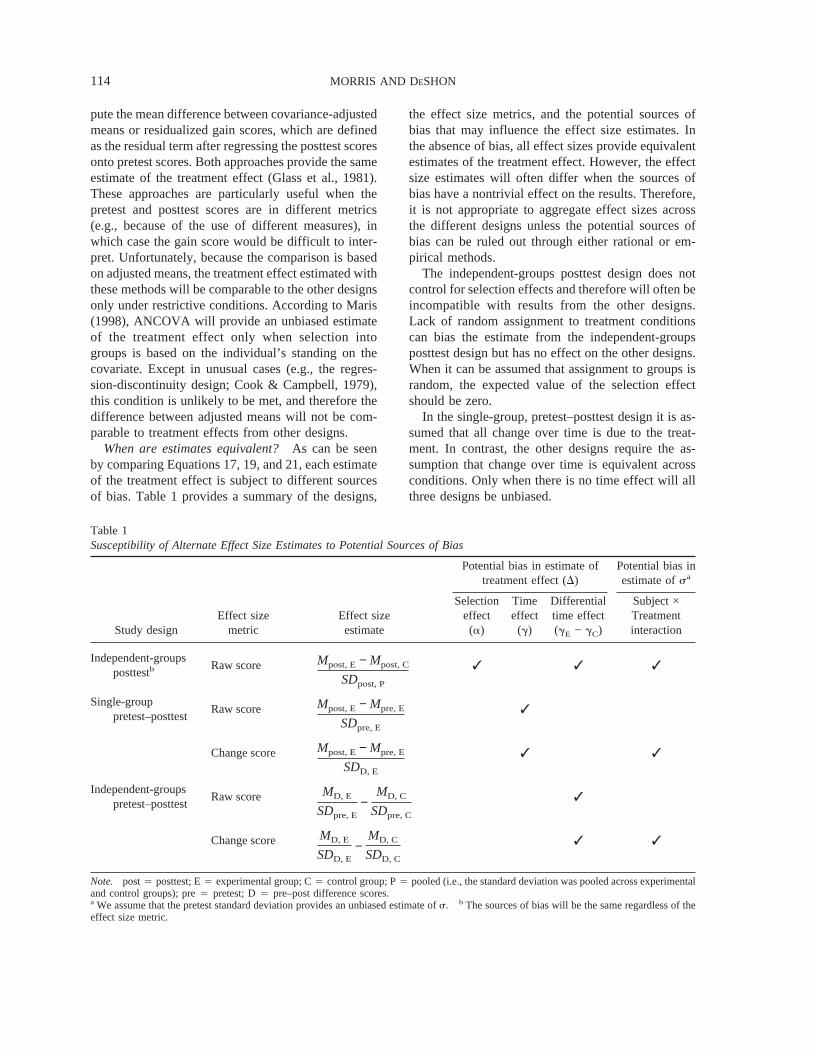
When are estimates equivalent?As can be seenby comparing Equations 17, 19, and 21, each estimateof the treatment effect is subject to different sourcesof bias. Table 1 provides a summary of the designs,

the effect size metrics, and the potential sources ofbias that may influence the effect size estimates. Inthe absence of bias, all effect sizes provide equivalentestimates of the treatment effect. However, the effectsize estimates will often differ when the sources ofbias have a nontrivial effect on the results. Therefore,it is not appropriate to aggregate effect sizes acrossthe different designs unless the potential sources ofbias can be ruled out through either rational or em-pirical methods.

The independent-groups posttest design does notcontrol for selection effects and therefore will often beincompatible with results from the other designs.Lack of random assignment to treatment conditionscan bias the estimate from the independent-groupsposttest design but has no effect on the other designs.When it can be assumed that assignment to groups israndom, the expected value of the selection effectshould be zero.

In the single-group, pretest–posttest design it is as-sumed that all change over time is due to the treat-ment. In contrast, the other designs require the as-sumption that change over time is equivalent acrossconditions. Only when there is no time effect will allthree designs be unbiased.

Table 1Susceptibility of Alternate Effect Size Estimates to Potential Sources of Bias

Study designEffect size

metricEffect sizeestimate

Potential bias in estimate oftreatment effect (D)

Potential bias inestimate ofsa

Selectioneffect(a)

Timeeffect(g)

Differentialtime effect(gE − gC)

Subject ×Treatmentinteraction

Independent-groupsposttestb

Raw score Mpost, E− Mpost, C

SDpost, P

✓ ✓ ✓

Single-grouppretest–posttest

Raw score Mpost, E− Mpre, E

SDpre, E

✓

Change score Mpost, E− Mpre, E

SDD, E

✓ ✓

Independent-groupspretest–posttest

Raw score MD, E

SDpre, E−

MD, C

SDpre, C

✓

Change score MD, E

SDD, E−

MD, C

SDD, C

✓ ✓

Note. post4 posttest; E4 experimental group; C4 control group; P4 pooled (i.e., the standard deviation was pooled across experimentaland control groups); pre4 pretest; D4 pre–post difference scores.a We assume that the pretest standard deviation provides an unbiased estimate ofs. b The sources of bias will be the same regardless of theeffect size metric.


In many areas of research, it is unrealistic to as-sume that there will be no time effect in the controlgroup. For example, if change over long periods oftime is looked at in a study, it is very likely thatmaturation or history effects would occur, suggestingthat the time effect will be nonzero. Research on psy-chotherapy (Lipsey & Wilson, 1993) and training(Carlson & Schmidt, 1999) frequently demonstratesnonzero change in the control group.

However, in other domains, there may be no reasonto expect a change absent treatment. In experimentalresearch comparing performance of the same subjectunder different conditions, many researchers usecounterbalancing of conditions, so that the mean dif-ference between treatments will not be influenced bythe order of presentation. A time effect would havethe same impact on treatment and control groupmeans and therefore would not bias the estimate of thetreatment effect. Other research applies repeated mea-sures over relatively short periods of time under con-trolled laboratory conditions. In such cases, matura-tion or history should have little effect. For example,in a meta-analysis on the effects of self-reference onmemory (Symons & Johnson, 1997), studies using asingle-group pretest–posttest design produced a meaneffect size that was very close to the estimate fromstudies that included a control group.

Furthermore, the assumption of no change in thecontrol group may be viable for variables that areresistant to spontaneous change. For example, in ameta-analysis on psychological treatments for insom-nia, Murtagh and Greenwood (1995) combined stud-ies using both the independent-groups posttest designand the single-group pretest–posttest design. The au-thors argued that it was appropriate to aggregate effectsizes across these two designs, because spontaneousrecovery from chronic insomnia is unlikely to occur.This decision was supported by their results, whichshowed a similar mean effect size across designs.Similarly, in a meta-analysis of training studies, Carl-son and Schmidt (1999) found changes in the controlgroup for some variables, but no substantial changewas found for measures of trainee attitudes.

Even when time effects occur, effect sizes can becombined across designs under certain conditions.When there is an equivalent time effect across groups,both designs involving independent groups will beunbiased and therefore can be combined. This wouldbe reasonable if the time effect was due to maturationand group assignment was unrelated to maturationrates.

Other types of time effects, such as fatigue, may berelated to the treatment, and therefore it may not beappropriate to assume equivalence across groups. Insuch cases, it may be reasonable to assume no timeeffect in the control group. With this assumption, ef-fect sizes from the single group pretest–posttest andindependent-groups pretest–posttest designs can becombined, although both will be biased estimates ofthe treatment effect.

In addition to the sources of bias discussed in thissection (selection, time, and differential time effects),Table 1 also indicates susceptibility to bias producedby a subject by treatment interaction. This form ofbias will not affect the estimation of the treatmenteffect, but it can bias the estimation of the standarddeviation as discussed in theComparability of Metricssection. Because the subject by treatment interactionwill inflate or deflate posttest variance, any effect sizethat uses posttest standard deviations is susceptible tothis form of bias. Effect sizes from the single-grouppretest–posttest and the independent-groups pretest–posttest designs will be unbiased if computed in theraw-score metric (using pretest standard deviations)but will be susceptible to bias when computed in thechange-score metric. Results from the independent-groups posttest only design will be susceptible to thisbias regardless of the metric of the effect size, becauseonly posttest standard deviations would be available(Carlson & Schmidt, 1999).

An alternative way to justify aggregation of effectsizes across designs would be to determine empiri-cally whether alternate designs provide similar esti-mates of the effect size. As a first step in a meta-analysis, a moderator test could be performed tocompare effect sizes across designs. If the mean effectsizes differ substantially, then separate analysesshould be performed for each design. However, ifsimilar mean effect size estimates are found for thealternate designs, they could be combined into asingle meta-analysis. Of course, it would also be pos-sible that differences in the bias in the various esti-mators would be confounded by differences in otherstudy characteristics. As a means of getting aroundthis problem, the study design could be used as one ofseveral moderators analyzed simultaneously in themeta-analysis (Hedges & Olkin, 1985).

Correcting for sources of bias.Often, it will notbe possible to assume that potential biasing factorshave no effect. In some cases, it may still be possibleto integrate effect sizes across designs if the relevantsources of bias can be estimated from the available


data. One of the advantages of aggregating resultsacross studies is that the strengths of one study cancompensate for the weaknesses of another. If somestudies provide adequate data to estimate a potentialsource of bias, this estimate can be applied to otherstudies in order to obtain unbiased estimates of theeffect size in all studies.

Consider a meta-analysis in which some of thestudies use a single-group pretest–posttest design andothers have an independent-groups pretest–posttestdesign. Whenever there is a nonzero pretest–posttestchange in the control group (gC), effect sizes from thetwo designs will estimate different parameters. If itcan be assumed that the time effect (g) is the same forthe treatment and control groups, the independent-groups pretest–posttest design will provide an unbi-ased estimate of the population effect size, whereasthe single-group pretest–posttest design will overesti-mate the effect of treatment. However, when suffi-cient information is available, it is possible to obtainan unbiased estimate using effect sizes from both de-signs.

Becker (1988) described two methods that can beused to integrate results from single-group pretest–posttest designs with those from independent-groupspretest–posttest designs. In both cases, meta-analyticprocedures are used to estimate the bias due to a timeeffect. The methods differ in whether the correctionfor the bias is performed on the aggregate results orseparately for each individual effect size. The twomethods are briefly outlined below, but interestedreaders should refer to Becker (1988) for a more thor-ough treatment of the issues.

The first approach would be to aggregate the pre-test–posttest effect sizes separately for the treatmentand control groups. For each independent-groups pre-test–posttest study, one effect size would be computedbased on the pre- and posttest means of the treatmentgroup, and a separate effect size would be computedbased on the pre- and posttest means for the controlgroup. The single-group pretest–posttest designwould only provide an effect size for the treatmentgroup. In order to account for the fact that multipleeffect sizes are included from the same study, a mixedmodel analysis could be used to estimate the meanstandardized pretest–posttest change for the treatmentand control groups. The result for the control groupprovides an estimate of the time effect, and the dif-ference between the two estimates provides an unbi-ased estimate of the population effect size. A similarmethod has been suggested by Li and Begg (1994).

A disadvantage of this method is that separate ef-fect size estimates are required for treatment and con-trol groups. Therefore, it would not be possible tointegrate these results with effect sizes from studiesusing an independent-groups posttest design. UsingBecker’s (1988) second method, it may be possible tocombine results from all three designs.

Rather than correcting for bias at the aggregatelevel, it is also possible to introduce a bias correctionfor individual studies. A preliminary meta-analysiswould be conducted on control groups from the stud-ies with independent-groups pretest–posttest designs.The mean standardized pretest–posttest change fromthese studies provides an estimate of the time effect(gC). If this time effect is assumed to be the same inthe treatment condition, then the mean time effect canbe subtracted from each of the effect size estimates forthe single-group pretest–posttest designs. As a result,both designs will provide an unbiased estimate of thetreatment effect. Furthermore, under conditions inwhich the independent-groups posttest design providesan unbiased estimate of the treatment effect, effect sizesfrom all three designs will be comparable and couldtherefore be combined in the same meta-analysis.

Because this method uses the results from one setof studies to estimate the correction factor for otherstudies, the effect size estimates will not be indepen-dent. Therefore, standard meta-analysis models,which assume independence, will not be appropriate.Consequently, Becker (1988) recommended the useof a generalized weighted least squares model for ag-gregating the results.

An important assumption of this method is that thesource of bias (i.e., the time effect) is constant acrossstudies. This assumption should be tested as part ofthe initial meta-analysis used to estimate the pretest–posttest change in the control group. If effect sizes areheterogeneous, the investigator should explore poten-tial moderators, and if found, separate time effectscould be estimated for subsets of studies.

Similar methods could be used to estimate and con-trol for other sources of bias. For example, Shadish etal. (2000) conducted a separate meta-analysis on thedifference between pretest scores for treatment andcontrol groups. This pretest effect size provided anestimate of the degree of bias resulting from nonran-dom assignment.

Sampling Variance Estimates

Sampling variancerefers to the extent to which astatistic is expected to vary from study to study, sim-


ply as a function of sampling error. Estimates of sam-pling error are used in a meta-analysis when comput-ing the mean and testing the homogeneity of effectsizes. Sampling variance is largely a function of thesample size but is also influenced by the study design.For example, whenr is large, the repeated measuresdesign will provide more precise estimates of popu-lation parameters, and the resulting effect size willhave a smaller sampling variance.

Variance formulas have been developed for boththe independent-groups (Hedges, 1981) and repeatedmeasures effect size (Gibbons et al., 1993). In addi-tion, Becker (1988, cf. Morris, 2000) and Hunter andSchmidt (1990) have developed slightly different for-mulas for an effect size in the raw-score metric esti-mated from repeated measures data. Rather than re-lying on these separate formulas, we present a generalform of the variance that encompasses the three ex-isting procedures, as well as a new situation, that is,an effect size in the change-score metric estimatedfrom an independent-groups posttest design.

The general form for the sampling variance (s2ei

)for an effect size in either metric is

sei

2 = SA2

ñ DS df

df − 2DS1 +ñ

A2 d*2D −

d*2

@c~df !#2. (22)

The derivation of this formula is presented in Appen-dix A. Each of the variables in Equation 22 can takeon different values, based on the design of the study

and the metric of the effect size.d* refers to the popu-lation effect size in the metric chosen for the meta-analysis. The bias functionc(df) is approximated bythe following (Hedges, 1982):

c~df ! = 1 −3

4 df − 1. (23)

When the data are from an independent-groupsposttest design,ñ4 (nE * nC)/(nE + nC), anddf 4 nE

+ nC − 2. If the data are from a single-group pretest–posttest design,ñ is the number of paired observa-tions, anddf 4 n − 1. In addition, if the result isexpressed in a different metric than the original de-sign, the appropriate transformation (as illustrated inEquations 11 and 12) is substituted for A. The result-ing variance for each type of effect size is indicated inTable 2.

The sampling variance formulas are somewhatmore complex when the effect size is estimated froman independent groups pretest–posttest design. Asshown in Equation 6, separate effect size estimateswould be calculated for the treatment and controlgroups. The difference between these two compo-nents effect sizes provides the best estimate of theoverall effect size for the study. The variance of thiscombined effect size is equal to the sum of the vari-ances for the two components (Becker, 1988). Thus,the variance would be estimated for each group, usingthe appropriate equation from Table 2, and thensummed.

Table 2Sampling Variance of the Effect Size as a Function of the Study Design and the Metric Used in the Meta-Analysis

Study design Effect size metric Sampling variance


Change score S1

nD Sn − 1

n −3D ~1 + ndRM2 ! −

dRM2

@c~n − 1!#2


Raw score F2 ~1 − r!

n G Sn − 1

n −3D F1 +n

2 ~1 − r!dIG

2 G −dIG

2

@c~n − 1!#2

Independent-groupsposttest

Raw score S1

ñD SN − 2

N −4D ~1 + ñdIG2 ! −

dIG2

@c~N − 2!#2

Independent-groupsposttest

Change score F 1

2 ~1 − r! ñG SN − 2

N −4D @1 + 2 ~1 − r! ñdRM2 # −

dRM2

@c~N − 2!#2

Note. nis the number of paired observations in a single–group pretest–posttest design;dRM anddIG are the population effect sizes in thechange-score and raw-score metrics, respectively;c(df ) is the bias function defined in Equation 23;ñ 4 (nE * nC)/(nE + nC); N is the combinednumber of observations in both groups (nE + nC).


Operational Issues in Estimating Effect Sizes

Estimating the Pretest–Posttest Correlation

Transforming effect sizes into alternate metrics re-quires an estimate of the population correlation be-tween pre- and posttest scores. Others have avoidedthis step by computing the independent-groups effectsize from means and standard deviations (Becker,1988; Dunlap et al., 1996; Hunter & Schmidt, 1990).However, the pretest–posttest correlation is also usedin the estimate of the sampling variance and thereforewill have to be estimated regardless of which ap-proach is used. In addition, it may be possible toestimater from studies in which sufficient data areavailable and to generalize this estimate to other stud-ies. This is similar to common procedures for estimat-ing study artifacts (e.g., reliability) based on incom-plete information in primary research reports (Hunter& Schmidt, 1990). Thus, the analyst would first per-form a preliminary meta-analysis on the pretest–posttest correlations and then use the result as thevalue ofr in the transformation formula. A variety ofmethods exist to aggregate correlation coefficientsacross studies, involving various corrections, weight-ing functions, and so forth (e.g., Hedges & Olkin,1985; Hunter & Schmidt, 1990; Rosenthal, 1991). Wedo not advocate any particular approach but ratherrely on the meta-analyst to determine the most appro-priate methods for the estimation ofr.

It is not necessary to assume that a single value ofr is appropriate for all studies. Some may feel thatrwill change as a function of study characteristics, suchas the length of time between pre- and posttest mea-sures (Dunlap et al., 1996). A test for homogeneity ofeffect size (Hedges & Olkin, 1985) can be used toevaluate whether the estimates ofr are consistentacross studies. If this test is significant, the differencesin r could be modeled as part of the initial meta-analysis, and then appropriate values estimated foreach study.

As noted earlier, the homogeneity ofr also hasimplications for the choice of an effect size metric.Effect sizes defined in the change-score metric shouldbe combined only for studies wherer is the same. Touse the change-score metric whenr varies acrossstudies, the researcher should perform separate meta-analyses for subsets of studies that have homogeneousr. Alternatively, the meta-analysis could be conductedin the raw-score metric, which is not affected byvariations inr.

Although the pretest–posttest correlation may not

be included in all study reports, it is often possible tocompute this value from available data. If boththe pre- and posttest standard deviations (SDpre andSDpost) are known, as well as the standard deviation ofdifference scores (SDD),

r =SDpre

2 + SDpost2 − SDD

2

~2! ~SDpre! ~SDpost!(24)

can be used to compute the pretest–posttest correla-tion. If the pre- and posttest standard deviations arenot known,r can also be estimated from the pooledstandard deviation (SDP),

r = 1 −SDD

2

2SDP2. (25)

The derivations of Equations 24 and 25 are presentedin Appendix B.

If the variance of difference scores is not reported,it can often be computed from test statistics and thensubstituted into one of the above equations. For ex-ample, if the means, sample size, and repeated mea-surest test (tRM) are reported,

SDD2 =

n~Mpost− Mpre!2

tRM2 . (26)

Estimating Effect Sizes From Test Statistics

If the means and standard deviations are unavail-able, the effect size can also be computed from teststatistics, using familiar conversion formulas. Whenan independent-groupst test is reported (tIG), the in-dependent-groups effect size estimate can be com-puted as follows (Glass et al., 1981):

dIG = tIGÎnE + nC

nEnC, (27)

wherenE and nC are the sample sizes from the twotreatment conditions. Similarly, the repeated measurest test (tRM) can be transformed into a repeated mea-sures effect size (Rosenthal, 1991),

dRM =tRM

=n, (28)

wheren is the number of individuals or matched pairsin the experiment.

For studies with an independent-groups pretest–posttest design, the effect size can be computed fromtest statistics, as long as the designs provide equiva-lent estimates of the treatment effect. The estimate


depends on the particular statistical test used. If at testwas computed on the difference between treatment-and control-group gain scores, then the repeated mea-sures effect size can be estimated using

dRM = tgainÎnE + nC

nEnC. (29)

An equivalent test would be to conduct a 2 × 2ANOVA with one between-groups factor (experimen-tal vs. control group) and one repeated factor (pre- vs.posttest). The square root of theF test on the group bytime interaction is equivalent totgainand therefore canbe substituted into Equation 29. Because theF valuedoes not indicate the direction of the difference, themeta-analyst must also specify whether the effect sizeis positive or negative, depending on the pattern ofmeans. For larger factorial designs, adjustments forthe other factors should also be considered (Cortina &Nouri, 2000).

If the data were analyzed using residualized gainscores or ANCOVA, the significance test will bebased on the difference between adjusted means, andtherefore it will not be possible to estimate the effectsize for unadjusted means from the significance test.As noted above, the difference between adjustedmeans will often not estimate the same treatment ef-fect as other designs. However, in cases in which theestimates are deemed to be comparable, Glass et al.(1981) provided formulas for estimating the indepen-dent-groups effect sizes from statistical tests. If at teston the difference in residualized gain scores (tr) isreported,

dIG = trÎ~1 − r2!SnE + nC

nEnCD . (30)

The F test from an ANCOVA can be translated intoan independent-groups effect size using

dIG = 2ÎF~1 − r2!~dfw − 1!

~nE + nC!~dfw − 2!, (31)

where dfw is the residual within-groups degrees offreedom.

Conducting the Meta-Analysis

Meta-analysis on effect sizes from alternate designscan be performed using standard procedures, as longas (a) the effect sizes are first transformed into a com-mon metric and (b) the appropriate sampling varianceformulas are used when estimating the mean and test-

ing for homogeneity of effect size. We present meth-ods for the fixed-effects model (Hedges & Olkin,1985). The procedures can be readily generalized torandom-effects models as well (Hedges & Vevea,1998).

The population effect size is generally estimatedfrom a weighted mean of the effect size estimates.The rationale for weighting is to allow more preciseestimates to have greater influence on the mean. If aneffect size has a small sampling variance, values arelikely to fall close to the population parameter. On theother hand, if the sampling variance is large, an indi-vidual estimate can differ substantially from the popu-lation effect size simply because of sampling error.By giving greater weight to more precise estimates,the resulting mean will be more accurate (i.e., will beless biased and have a smaller mean square error;Hedges & Olkin, 1985).

Precision is largely a function of the sample size;larger samples produce more precise estimates. As aresult, some have recommended weighting by samplesize (Hunter & Schmidt, 1990). When all studies arefrom the same design, this produces an average effectsize that is very close to the optimal precision-weighted estimate (Hedges & Olkin, 1985). However,when multiple designs are included, both the designand the sample size influence precision. For example,in a repeated measures design, each participant istreated as his or her own control, thereby reducingerror variance due to individual differences. Thesmaller error variance results in a more precise esti-mate of the mean difference and, consequently, amore precise effect size estimate.

The mean effect size will be most accurate whenthe estimates from the individual studies are weightedby the reciprocal of the sampling variance (Hedges &Olkin, 1985). In addition, because the design influ-ences the formula for the sampling variance, varianceweighting accounts for both sample size and studydesign. The variance-weighted mean effect size is

d =(

i

widi

(i

wi

, (32)

where the weights (wi) are defined as the reciprocal ofthe sampling variance (1/s2

ei) estimated from Equa-

tion 22.As Hedges (1982) noted, an inherent problem in

meta-analysis is that it is necessary to know the popu-lation effect size in order to estimate the sampling


variance, which in turn is needed to estimate thepopulation effect size. This problem can be solved byfirst computing an unweighted average effect size andthen using this value as the estimate ofd in the vari-ance formula. These variance estimates are then usedto compute the weighted mean effect size using Equa-tion 32.

Differences in study designs must also be taken intoaccount in tests for homogeneity of effect size. Testsfor homogeneity are based on the comparison of theobserved variance of the effect size (sd

2) to the theo-retical variance due to sampling error (se

2). Again, theeffect of study design will be incorporated by usingappropriate formulas for the sampling variance. Aswith the mean, variance-weighted estimates are gen-erally used. Thus, the observed variance is

sd2 =

(i

wi ~di − d!2

(i

wi

, (33)

wherewi 4 1/sei

2 . The variance due to sampling erroris estimated from the weighted average of the indi-vidual study variances, or

se2 =

(i=1

k

wi sei

2

(i=1

k

wi

=k

(i=1

k 1

sei

2

, (34)

wherek is the number of studies in the meta-analysis.Once the design effects have been taken into ac-

count in the estimates ofsd2 andse

2, standard tests forhomogeneity proceed normally. Using the Hunter andSchmidt (1990) 75% rule, the effect size would beviewed as homogeneous if

se2

sd2 . .75. (35)

Alternatively, Hedges (1982) recommended evaluat-ing homogeneity of effect size with a significancetest, which can be written as

Q =ksd

2

se2 . (36)

TheQ statistic is tested against a chi-square distribu-tion with k-1 degrees of freedom.

TheQ statistic can also be used to test for categori-cal moderators of the effect size. A separate test sta-

tistic (Qj) is computed for studies within each of theJlevels of the moderator, as well as the overall statisticfor all studies (QT). The difference between levels ofthe moderator can be tested using a between-groupsstatistic (QB), where

QB = QT − (j=1

J

Qj (37)

with df 4 J − 1. Methods for simultaneous analysis ofmultiple moderators are described in Hedges andOlkin (1985).

As an example, a small meta-analysis of the inter-personal skills training literature was performed. Forpurposes of illustration, separate meta-analyses wereconducted using both the raw-score and the change-score metrics. This is not recommended in practice,where a single meta-analysis should be conducted us-ing the metric that best addresses the research ques-tion.

Table 3 presents 15 effect sizes addressing the ef-ficacy of interpersonal skills training taken from 10studies. The first step in this meta-analysis was todetermine the design used and the relevant samplesize information for each computed effect size. Thefirst column in Table 3 contains the author of thestudy. The second column identifies the design usedin the study. Nine of the effect sizes were based onsingle-group pretest–posttest designs and the remain-ing 6 used independent-groups posttest designs. Thethird and fourth columns contain sample size infor-mation for the groups (these numbers may be unequalfor independent-groups posttest designs).

After identifying the design, the effect size esti-mates were computed. For the independent-groupsposttest designs this computation was based on Equa-tion 2 (if descriptive statistics were available) orEquation 27 (if at test orF test was available). Foreffect sizes taken from single-group pretest–posttestdesigns, Equation 4 or Equation 28 was used, depend-ing on whether descriptive statistics were available.

Next, Equations 11 and 12 were used to converteffect sizes from the independent-groups postteststudies into the change-score metric, and effect sizesfrom the single-group pretest–posttest studies into theraw-score metric, so that the results of each studywere computed in each metric. Again, this step wasperformed only to illustrate the procedure, and onlyone metric should be used in practice. A small com-plication arises when making these transformations.Both Equation 11 and Equation 12 require informa-


tion concerning the population correlation betweenthe repeated measures. As discussed earlier, we be-lieve that an aggregate of the correlational data acrossthe single-group pretest–posttest designs provides thebest estimate of the population correlation. Therefore,a small meta-analysis of the correlations across thesingle-group pretest–posttest studies was undertaken.Only the last four studies in Table 3 contained suffi-cient information to estimate the correlation of re-sponses across time (.69, .72, .55, and .58). UsingHedges and Olkin’s (1985) method to meta-analyzethese correlations yielded a variance-weighted aver-age correlation of .61. Before incorporating this esti-mate of the correlation into our analysis, the homo-geneity of the correlations was examined. TheQ testyielded a nonsignificant chi-square result,x2(3, N 4245)4 3.26,p > .05, indicating that the null hypoth-esis of homogeneity was not rejected.

The raw-score and change-score effects sizes foreach study are presented in the fifth and sixth columnsof Table 3. Notice that the change-score effect sizesare uniformly larger than the raw-score effect sizes, aswill generally be the case.

Once the effect sizes were computed, the next stepin the meta-analysis was to estimate the samplingvariance of each effect size. In addition to the valuesalready computed, two additional pieces of informa-tion were required to use these formulas—the biasfunction,c, and the population effect size. The valuefor the bias function,c, may be computed for botheffect size metrics using Equation 23.

There are many alternative ways to estimate thepopulation effect size needed to compute the samplingvariance. For most purposes, the simple average of theeffect sizes in Table 3 serves as a reasonable estimateof this parameter. Across all 15 effect sizes, the av-

Table 3Example of a Meta-Analysis Based on Raw-Score and Change-Score Effect Sizes

Study Design n1 n2 dIG dRM c

Raw-score metric Change-score metric

VarIG wIG wIG * dIG VarRM wRM wRM * dRM

Smith-Jentsch, Salas,and Baker (1996)

IG 30 30 0.61 0.69 0.99 0.08 13.12 8.04 0.10 10.30 7.09

Smith-Jentsch, Salas,and Baker (1996)

IG 30 30 0.89 1.00 0.99 0.08 13.12 11.62 0.10 10.30 10.25

Moses and Ritchie(1976)

IG 90 93 0.96 1.07 1.00 0.02 41.15 39.34 0.03 32.29 34.68

Fiedler and Mahar(1979)

IG 9 9 1.34 1.51 0.95 0.29 3.50 4.70 0.36 2.75 4.14

Fiedler and Mahar(1979)

IG 190 215 0.26 0.29 1.00 0.01 91.42 23.59 0.01 71.74 20.80

Engelbrecht andFischer (1995)

IG 41 35 0.52 0.59 0.99 0.06 16.67 8.69 0.08 13.08 7.65

Leister et al. (1977) RM 27 27 0.75 0.84 0.97 0.05 20.45 15.36 0.06 16.09 13.58Leister et al. (1977) RM 27 27 0.50 0.57 0.97 0.05 20.45 10.31 0.06 16.09 9.11R. M. Smith, White,

and Montello (1992)RM 12 12 1.25 1.40 0.93 0.13 7.60 9.48 0.17 5.98 8.38

R. M. Smith, White,and Montello (1992)

RM 12 12 1.10 1.23 0.93 0.13 7.60 8.32 0.17 5.98 7.35

P. E. Smith (1976) RM 36 36 2.89 3.25 0.98 0.04 28.13 81.30 0.05 22.14 71.96Gist et al. (1991) RM 44 44 0.84 0.94 0.98 0.03 34.96 29.33 0.04 27.51 25.94Gist et al. (1991) RM 35 35 0.83 0.93 0.98 0.04 27.28 22.61 0.05 21.46 20.00Campion and Campion

(1987)RM 127 127 0.38 0.43 0.99 0.01 105.74 40.50 0.01 83.19 35.77

Harris and Fleishmann(1955)

RM 39 39 0.11 0.13 0.98 0.03 30.69 3.44 0.04 24.15 3.04

Note. n1 andn2 are the sample sizes in the experimental and control group or the first and second time period, depending on the experimentaldesign;d is the effect size estimate;c is the bias function in Equation 23; Var is the estimated sampling variance of the effect sizes;w is thevalue used to weight the effect size estimates. IG4 independent groups; RM4 repeated measures. The statistics are reported for both theraw-score and change-score effect sizes as indicated by the subscripts IG and RM, respectively.


erage raw-score effect size was 0.882 and the averagechange-score effect size was 0.991.

The sampling variance of each effect size was es-timated using the equations in Table 2 and the valuesjust presented. As shown in Table 2, different equa-tions were required depending on the original studydesign and whether the effect size was analyzed in theoriginal metric or transformed. Equation 32 was usedto estimate the variance-weighted mean effect size.The weights were defined as the reciprocal of thesampling variance for each effect size estimate. Onthe basis of the values in Table 3, the effect sizes werecomputed by taking the sum of the column represent-ing the weighted effect sizes and dividing by the sumof the column representing the weights. For thechange-score effect sizes this equation yielded a valueof 0.77, and for the raw-score effect sizes this valuewas 0.69. As expected, the effect size was slightlylarger in the change-score metric than in the raw-scoremetric. In either case, the results indicate a moderatelylarge improvement due to training.

Next, effects sizes were tested for homogeneity.Sampling variance accounted for only a small propor-tion of the observed variance in effect sizes (.08 forboth effect size metrics), which falls far below theHunter and Schmidt (1990) 75% rule (Equation 35).Thus, for both metrics, there was substantial variancein the effect size estimates that could not be attributedto sampling error. Hedges’ chi-square test of homo-geneity resulted in similar conclusions. The chi-square homogeneity test was significant for both theraw-score metric,x2(14, N 4 1161)4 184.90,p <.01, and the change-score metric,x2(14, N 4 1161)4 183.78,p < .01. As with the 75% rule, this meansthat there is evidence of heterogeneity among the ef-fect sizes, and a search for possible moderator vari-ables is warranted.

As noted earlier, different designs may be subjectto different sources of bias and therefore may notprovide comparable estimates of effect size. To ex-amine whether effect sizes could be aggregated acrossdesigns, we tested for study design as a moderator ofthe effect size. The moderator analysis was conductedusing the fixed-effects analysis described in Hedgesand Olkin (1985) for the raw-score metric. When con-sidered separately, the effect sizes from independent-groups posttest designs were heterogeneousx2(5, N4 802) 4 18.72,p < .05, as were the effect sizesfrom the single-group pretest–posttest designs,x2(8,N 4 359)4 149.96,p < .05. The variance-weightedaverage effect size (in the raw-score metric) was 0.78

for the single-group pretest–posttest designs and 0.54for the independent-groups posttest designs. The testof moderation indicated that the design was a signifi-cant moderator of the effect sizes,x2(1, N 4 1161)416.22,p < .05. Thus, there is evidence that even afteraccounting for differences in the effect sizes due tothe metric, the effect sizes still differ across the de-signs. Substantive or bias explanations would have tobe explored to identify the cause of this difference,and these effect sizes should not be combined in asingle estimate of the effect of training on interper-sonal skills.

Conclusion

When a meta-analyses is conducted, it is often de-sirable to combine results across independent-groupsand repeated measures designs. When effect sizes arecombined across these designs, it is critical that anumber of steps be followed. Appropriate transforma-tions must be used to ensure that all effect sizes are ina common metric. In addition, meta-analysis proce-dures should use design-specific sampling varianceformulas to specify the precision of effect size esti-mates. Finally, unless the researcher can justify, basedon rational analysis or empirical moderator analyses,that the alternate designs estimate the same treatmenteffect, the effect sizes from the two designs should notbe combined. This procedure provides maximal flex-ibility to the meta-analyst. Researchers can choose toanalyze effect sizes in either the raw-score or change-score metric, depending on which metric best reflectsthe pool of studies and the research question, and canreadily incorporate results from studies using differentdesigns.

A major challenge to this approach is the need tojustify that effect sizes from different designs estimatethe same treatment effect. Because different designscontrol for different types of bias, certain designs arelikely to over- or underestimate the treatment effect.The researcher can justify aggregation of effect sizesacross designs either rationally or empirically. De-pending on the nature of the process under investiga-tion and the specific experimental designs used, itmay be possible to rule out potential sources of bias,thereby allowing estimates to be compared across de-signs. For example, when an intervention is examinedover relatively short time periods, bias due to historyor maturation can be ruled out, and time effects can beassumed to be minimal. As a result, effect sizes fromindependent-groups and repeated measures designs


should estimate the same treatment effect. Thus, al-though the two designs are not comparable in general,they may be comparable in specific research domains.

The aggregation of effect sizes across designs couldalso be justified empirically. As a first step in con-ducting a meta-analysis, the researcher should test formean differences between the effect sizes from alter-nate designs. If systematic differences are found, re-sults from different designs must be analyzed sepa-rately. Alternately, the magnitude of various sourcesof bias could be estimated as part of the meta-analysis(Becker, 1988; Li & Begg, 1994; Shadish et al., 2000).However, if no differences between designs arefound, effect sizes could be combined. Naturally, thestrongest case for aggregation can be made when bothrational and empirical justification can be provided.

A limitation of the repeated measures effect size isthat it compares only two time periods. In many re-search areas in which the repeated measures effectsize would be of greatest interest (e.g., practice orlearning effects), it is often beneficial to observe thetrajectory of growth curves across multiple observa-tions (Keppel, 1982). The use of a single pretest–posttest comparison might miss important informationabout the shape of growth trajectories. However, itshould be noted that this problem is inherent in anymeta-analysis using standardized mean differences,not just the methods proposed here. Becker (1988)suggested that this could be addressed by computingmultiple comparisons within each study and then us-ing a meta-analysis procedure that models bothwithin- and between-studies effects.

Combining effect sizes estimated from studies us-ing different research designs is a challenging andoften time-consuming process. In this presentation,we detailed the methods required to appropriatelycombine effect sizes from repeated measures and in-dependent-groups designs and highlighted the infer-ential hazards that may be encountered when doingso. However, it should be emphasized that the diffi-culties highlighted above (e.g., differences in metricand differential susceptibility to bias) are not uniqueto combining effects sizes across dependent- and in-dependent-groups designs. In fact, virtually all ofthese issues should be considered when combiningeffect sizes across different independent-groups de-signs (cf. Morris & DeShon, 1997). We recommendthat when a meta-analysis is conducted, it should becommon practice to record differences in design andto examine experimental design as a moderator of theeffect sizes.

References

Becker, B. J. (1988). Synthesizing standardized mean-change measures.British Journal of Mathematical andStatistical Psychology, 41,257–278.

Burke, M. J., & Day, R. R. (1986). A cumulative study ofthe effectiveness of managerial training.Journal of Ap-plied Psychology, 71,232–245.

Campion, M. A., & Campion, J. E. (1987). Evaluation of aninterviewee skills training program in a natural field ex-periment.Personnel Psychology, 40,675–691.

Carlson, K. D., & Schmidt, F. L. (1999). Impact of experi-mental design on effect size: Findings from the researchliterature on training.Journal of Applied Psychology, 84,851–862.

Cook, T. D., & Campbell, D. T. (1979).Quasi-experimentation: Design and analysis issues for field set-tings.Boston: Houghton Mifflin.

Cortina, J. M., & DeShon, R. P. (1998). Determiningrelative importance of predictors with the observa-tional design.Journal of Applied Psychology, 83,798–804.

Cortina, J. M., & Nouri, H. (2000).Effect size for ANOVAdesigns.Thousand Oaks, CA: Sage.

Dilk, M. N., & Bond, G. R. (1996). Meta-analytic evalua-tion of skills training research for individuals with severemental illness.Journal of Consulting and Clinical Psy-chology, 64,1337–1346.

Dunlap, W. P., Cortina, J. M., Vaslow, J. B., & Burke, M. J.(1996). Meta-analysis of experiments with matchedgroups or repeated measures designs.PsychologicalMethods, 1,170–177.

Eagly, A. H., Makhijani, M. G., & Klonsky, B. G. (1992).Gender and the evaluation of leaders: A meta-analysis.Psychological Bulletin, 111,3–22.

Engelbrecht, A. S., & Fischer, A. H. (1995). The managerialperformance implications of a developmental assessmentcenter process.Human Relations, 48,387–404.

Fiedler, F. E., & Mahar, L. (1979). A field experiment vali-dating contingency model leadership training.Journal ofApplied Psychology, 64,247–254.

Fleishman, E. A., & Hempel, W. E., Jr. (1955). The relationbetween abilities and improvement with practice in a vi-sual discrimination reaction task.Journal of Experimen-tal Psychology, 49,301–312.

Gibbons, R. D., Hedeker, D. R., & Davis, J. M. (1993). Es-timation of effect size from a series of experiments in-


volving paired comparisons.Journal of Educational Sta-tistics, 18,271–279.

Gist, M. E., Stevens, C. K., & Bavetta, A. G. (1991). Effectsof self-efficacy and post-training intervention on the ac-quisition and maintenance of complex interpersonalskills. Personnel Psychology, 44,837–861.

Glass, G. V., McGaw, B., & Smith, M. L. (1981).Meta-analysis in social research.Beverly Hills, CA: Sage.

Guzzo, R. A., Jette, R. D., & Katzell, R. A. (1985). Theeffects of psychologically-based intervention programson worker productivity: A meta-analysis.Personnel Psy-chology, 38,275–291.

Harris, E. F., & Fleishmann, E. A. (1955). Human relationstraining and the stability of leadership patterns.Journal ofApplied Psychology, 39,20–25.

Hedges, L. V. (1981). Distribution theory for Glass’s esti-mator of effect size and related estimators.Journal ofEducational Statistics, 6,107–128.

Hedges, L. V. (1982). Estimation of effect size from a seriesof independent experiments.Psychological Bulletin, 92,490–499.

Hedges, L. V., & Olkin, I. (1985).Statistical methods formeta-analysis.San Diego, CA: Academic Press.

Hedges, L. V., & Vevea, J. L. (1998). Fixed- and random-effects models in meta-analysis.Psychological Methods,3, 486–504.

Hunter, J. E., & Schmidt, F. L. (1990).Methods of meta-analysis: Correcting error and bias in research findings.Newbury Park, CA: Sage.

Johnson, B. T., & Eagly, A. H. (2000). Quantitative synthe-sis of social psychological research. In H. T. Reis &C. M. Judd (Eds.),Handbook of research methods in so-cial and personality psychology(pp. 496–528). Cam-bridge, England: Cambridge University Press.

Kelsey, I. B. (1961). Effects of mental practice and physicalpractice upon muscular endurance.Research Quarterly,32, 47–54.

Keppel, G. (1982).Design and analysis: A researcher’shandbook(2nd ed.). Englewood Cliffs, NJ: Prentice Hall.

Leister, A., Borden, D., & Fiedler, F. E. (1977). Validationof contingency model leadership training: Leader match.Academy of Management Journal, 20,464–470.

Li, Z., & Begg, C. B. (1994). Random effects models forcombining results from controlled and uncontrolled stud-ies in a meta-analysis.Journal of the American StatisticalAssociation, 89,1523–1527.

Lipsey, M. W., & Wilson, D. B. (1993). The efficacy ofpsychological, educational, and behavioral treatment:Confirmation from meta-analysis.American Psycholo-gist, 48,1181–1209.

Maris, E. (1998). Covariance adjustment versus gainscores—Revisited.Psychological Methods, 3,309–327.

Morris, S. B. (2000). Distribution of the standardized meanchange effect size for meta-analysis on repeated mea-sures.British Journal of Mathematical and StatisticalPsychology, 53,17–29.

Morris, S. B., & DeShon, R. P. (1997). Correcting effectsizes computed from factorial ANOVA for use in meta-analysis.Psychological Methods, 2,192–199.

Moses, J. L., & Ritchie, R. J. (1976). Supervisory relation-ships training: A behavioral evaluation of a behavioralmodeling program.Personnel Psychology, 29,337–343.

Murtagh, D. R. R., & Greenwood, K. M. (1995). Identifyingeffective psychological treatments for insomnia: A meta-analysis.Journal of Consulting and Clinical Psychology,63, 79–89.

Neuman, G. A., Edwards, J. E., & Raju, N. S. (1989). Or-ganizational development interventions: A meta-analysisof their effects on satisfaction and other attitudes.Per-sonnel Psychology, 42,461–489.

Rambo, W. W., Chomiak, A. M., & Price, J. M. (1983).Consistency of performance under stable conditions ofwork. Journal of Applied Psychology, 68,78–87.

Ray, J. W., & Shadish, W. R. (1996). How interchangeableare different estimators of effect size?Journal of Con-sulting and Clinical Psychology, 64,1316–1325.

Rosenthal, R. (1991).Meta-analytic procedures for socialresearch(Rev. Ed.). Newbury Park, CA: Sage.

Shadish, W. R., Navarro, A. M., Matt, G. E., & Phillips, G.(2000). The effects of psychological therapies underclinically representative conditions: A meta-analysis.Psychological Bulletin, 126,512–529.

Smith, P. E. (1976). Management modeling training to im-prove morale and customer satisfaction.Personnel Psy-chology, 29,351–359.

Smith, R. M., White, P. E., & Montello, P. A. (1992). In-vestigation of interpersonal management training for ad-ministrators.Journal of Educational Research, 85,242–245.

Smith-Jentsch, K. A., Salas, E., & Baker, D. P. (1996).Training team performance-related assertiveness.Per-sonnel Psychology, 49,909–936.

Symons, C. S., & Johnson, B. T. (1997). The self-referenceeffect in memory: A meta-analysis.Psychological Bulle-tin, 121,371–394.

Taylor, M. J., & White, K. R. (1992). An evaluation of al-ternative methods for computing standardized mean dif-ference effect size.Journal of Experimental Education,61, 63–72.

Winer, B. J. (1971).Statistical principles in experimentaldesign.New York: McGraw-Hill.


Appendix A

Derivation of the Variance of the Independent-Groups and Repeated Measures Effect Size

Hedges (1981) and Gibbons et al. (1993) have derived thevariance of the independent-groups and repeated measureseffect size, respectively. In both cases, normality and ho-mogeneity of variance across populations are assumed. Bothderivations resulted in the same equation for the samplingvariance, except for differences in the effect size parameter(dIG or dRM, both referred to asd* here),n, anddf,

sei2 = S1

nDS df

df−2D~1 + n d*2! −

d*2

c~df !2. (A1)

For the independent-groups effect size,df 4 nE + nC − 2and

n =nEnC

nE + nC. (A2)

For the repeated measures effect size,df 4 n − 1, andñ 4 n.

If the effect size is transformed by a multiplicative con-stant (dT 4 A d*), the variance will be A2 times the vari-ance of the original effect size. The variance will be a func-tion of the population effect size in the original metric (d*).However, for consistency, the equation should be presentedin terms of the chosen metric. This can be accomplished byreplacingd* with dT/A. Thus, the variance of the trans-formed effect size is as follows:

se = A2FS1

nDS df

df − 2DS1 + ndT

2

A2D +dT

2 /A2

c~df !2G

= SA2

n DS df

df − 2DS1 +n

A2dT

2D −dT

2

c~df !2. (A3)

Appendix B

Estimation of Pretest–Posttest Correlation From Standard Deviations

The variance of the difference scores (SDD2 ) can be writ-

ten as a function of the pre- and posttest variances (SD2pre

andSD2post) and the pretest–posttest correlation (r):

SD2D 4 SD2

pre + SD2post − (2) (r) (SDpre) (SDpost). (B1)

Solving for r, we obtain

r =SDpre

2 + SDpost2 − SDD

2

~2!~SDpre!~SDpost!. (B2)

If it is assumed that the pre- and posttest variances are bothequal to the pooled variance (SDP

2), Equation B2 reduces to

r = 1 −SDD

2

2SDP2. (B3)

Received June 13, 2000Revision received April 15, 2001

Accepted August 21, 2001■


combining effect size estimates in meta-analysis...

Documents