combining fixed- and moving-vessel acoustic doppler · pdf filecombining fixed- and...

Combining fixed- and moving-vessel acoustic Doppler current profilermeasurements for improved characterization of the mean flow in anatural river

John Petrie,1 Panayiotis Diplas,2 Marte Gutierrez,3 and Soonkie Nam4

Received 14 March 2013; revised 13 June 2013; accepted 1 July 2013.

[1] A methodology is presented to quantify the mean flow field in a natural river with aboat-mounted acoustic Doppler current profiler (ADCP). Moving-vessel (MV) and fixed-vessel (FV) survey procedures are used in a complementary fashion to provide an improvedrepresentation of mean three-dimensional velocity profiles along a cross section. Meanvelocity profiles determined with FV measurements are rotated to a stream-fitted orthogonalcoordinate system. The orientation of the coordinate system is established using MVmeasurements. The methodology is demonstrated using measurements obtained at twostudy sites on the lower Roanoke River for the mean annual flow (228 m3 s�1) and a flowthat produces bankfull conditions at the sites (565 m3 s�1). Results at a meander bendidentify well-known flow features, including a main circulation cell, outer-bank circulation,and separation at the inner bank. This methodology also provides a framework forcomparing time-averaged velocity profiles from FV measurements with spatially averagedprofiles from MV measurements. Results indicate that MV measurements can provide areasonable estimate of the streamwise velocity at many locations. The MV measurementsobtained here, however, were not sufficient to resolve the spanwise velocity component.

Citation: Petrie, J., P. Diplas, M. Gutierrez, and S. Nam (2013), Combining fixed- and moving-vessel acoustic Doppler currentprofiler measurements for improved characterization of the mean flow in a natural river, Water Resour. Res., 49, doi :10.1002/wrcr.20396.

1. Introduction

[2] The flow field in natural rivers is characterized byturbulent three-dimensional (3-D) velocity. The 3-D natureof velocity is due to channel planform curvature and pro-nounced channel topography [e.g., Rozovskii, 1957; Die-trich and Smith, 1983] as well as anisotropic turbulence[Tominaga et al., 1989]. To interpret field data, velocitymeasurements are often decomposed into orthogonal com-ponents in the streamwise, spanwise, and vertical direc-tions. Orientation of the horizontal components isdependent on the definition of the primary flow direction.Typically, the streamwise flow direction is prescribed usingeither channel geometry or flow characteristics. Velocitycomponents in the plane perpendicular to the streamwisedirection formed by the spanwise and vertical axes are

referred to as secondary velocities and are known to influ-ence channel morphology [e.g., Blanckaert, 2011] andecology [e.g., Shen and Diplas, 2008, 2010]. Interpretationof secondary velocity patterns is complicated due to thesmall magnitudes relative to the streamwise component aswell as when only the horizontal velocity is measured andvertical velocity must be inferred. Lane et al. [2000] advo-cated the use of 3-D computational fluid dynamics (CFD)models to directly represent velocity vectors as an alterna-tive to interpreting orthogonal components. Flows in natu-ral rivers are particularly challenging to model due to thepresence of moving boundaries, including both the channelboundary and free-surface, complex topography, turbu-lence, and boundary roughness. Despite these complexities,CFD has been applied to flows in natural rivers with prom-ising results [e.g., Ferguson et al., 2003; Shen and Diplas,2008, 2010; R€uther et al., 2010]. High-resolution field datafor boundary conditions and validation are needed to sup-port the expanding role of CFD in fluvial hydraulics.

[3] A boat-mounted acoustic Doppler current profiler(ADCP) is a versatile tool for riverine studies that can pro-vide measurements of 3-D velocity and channel topogra-phy. The spatial and temporal resolution of the velocitymeasurements is dependent on the type of deployment.During moving-vessel (MV) measurements, the ADCPrecords continuously while the boat traverses the channel.This is the most common boat-mounted survey procedureand provides accurate measurements of discharge [Obergand Mueller, 2007]. Fixed-vessel (FV) measurements areperformed while the boat is held at a constant position

1Department of Civil and Environmental Engineering, WashingtonState University, Pullman, Washington, USA.

2Imbt Environmental Hydraulics Laboratory, Department of Civil andEnvironmental Engineering, Lehigh University, Bethlehem, Pennsylvania,USA.

3Division of Engineering, Colorado School of Mines, Golden, Colorado,USA.

4Department of Civil and Environmental Engineering, South DakotaSchool of Mines and Technology, Rapid City, South Dakota, USA.

Corresponding author: J. Petrie, Department of Civil and Environmen-tal Engineering, Washington State University, 405 Spokane St., Sloan 101,Pullman, WA 99164-2910, USA. ([email protected])

©2013. American Geophysical Union. All Rights Reserved.0043-1397/13/10.1002/wrcr.20396

1

WATER RESOURCES RESEARCH, VOL. 49, 1–15, doi:10.1002/wrcr.20396, 2013

within the channel. The improved temporal resolution canbe used to determine mean (e.g., time-averaged) velocityprofiles [Petrie et al., 2013] and bed load velocity [Rennieet al., 2002]. Due to the increased effort required to collectFV measurements, several studies have investigated meanvelocity profiles from MV measurements using spatialaveraging or interpolation [Muste et al., 2004a, 2004b;Dinehart and Burau, 2005; Szupiany et al., 2007].Recently, kriging has been used to interpolate planformmaps of flow quantities, including depth-averaged velocity,boundary shear stress, and bed load velocity, from MVmeasurements [Rennie and Church, 2010; Guerrero andLamberti, 2011]. Jamieson et al. [2011] and Tsubaki et al.[2012] have extended this work to interpolate the 3-D ve-locity field. While these maps do not represent mean quan-tities in a strict time-averaged sense, Jamieson et al. [2011]argued that interpolated maps may better represent a com-plex flow field than averaging repeat transects that are notcoincident and introduce spatial averaging. Nonetheless, adetailed comparison of interpolated maps to time-averagedvelocities has yet to be reported.

[4] This study presents a methodology to quantify themean flow field in a natural river with a boat-mountedADCP using both MV and FV survey procedures. Thisapproach capitalizes on the relative advantage of each pro-cedure, with the MV measurements providing the directionof primary flow and channel topography while the FVmeasurements determine the mean velocity profiles. Acomparison of mean velocity profiles from FV and MVmeasurements is performed to determine if the MV meas-urements can quantify the spatial distribution of the meansecondary velocity. The methodology is then demonstratedby examining mean velocity profiles throughout a meanderbend.

2. Field Measurements

2.1. Study Sites

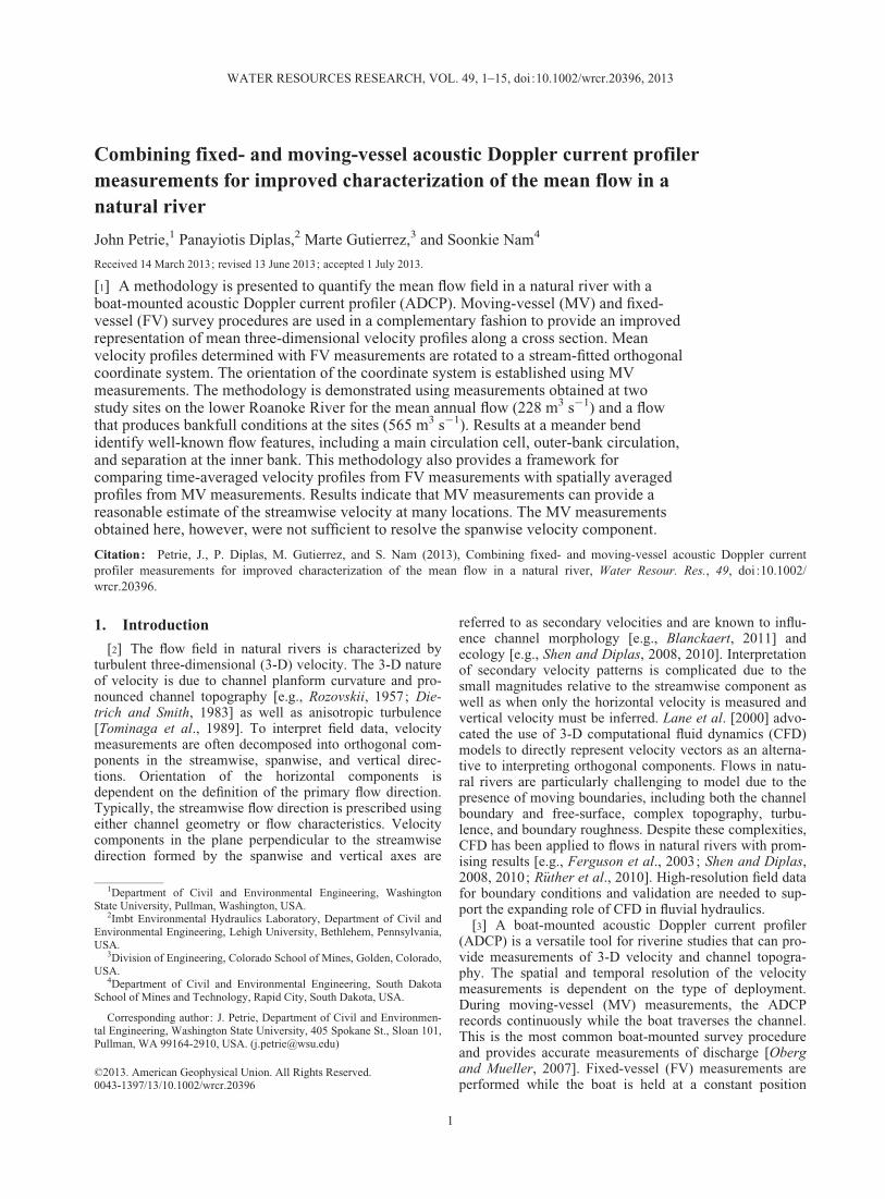
[5] ADCP measurements were obtained in May and June2009 at two study sites shown in Figure 1 on the lower Ro-anoke River in eastern North Carolina. Flow to the lowerreach is primarily controlled by releases from the RoanokeRapids Dam. The effect of this flow regulation on bankretreat has been the subject of recent investigations [Huppet al., 2009; Nam et al., 2010, 2011]. Reservoir releaseswere relatively steady for both survey periods, with the dis-charge Q in May close to the mean annual flow (Q¼ 228m3 s�1) and at bankfull in June (Q¼ 565 m3 s�1). Furtherinformation on the study sites and flow conditions is pro-vided in Petrie et al. [2013].

2.2. Equipment and Measurement Procedures

[6] The ADCP measures 3-D velocity components byapplying the Doppler principle to the frequency shift ofreflected acoustic pulses, called pings. Measurements areassigned to equally spaced discrete locations in the watercolumn, called bins. A bin size of 0.25 m was used for allmeasurements in this study. Limitations of the instrumentprevent velocity measurements from being obtained nearthe water surface or near the bed [see Simpson, 2001]. Anensemble is one measurement of the velocity profile andmay be composed of a single ping or the average of several

pings. For the FV measurements, 20 subpings sent 50 msapart were used to create each ensemble. The recom-mended settings provided by the ADCP software were usedfor the MV measurements. For the mean annual flow, thisresulted in seven subpings sent 40 ms apart to create an en-semble for most transects and one subping sent 70 ms apartfor most transects during the bankfull flow. Data were col-lected using Water Mode 12 and Bottom Mode 5 [seeMueller and Wagner, 2009]. Global positioning system(GPS) was used as the velocity reference for all measure-ments, with the exception of one FV measurement,S1xs6p2 (nomenclature is explained in the following sec-tion), during the mean annual flow, due to a problem withthe GPS signal. The decision to use GPS was based onobservations of bed movement, especially during the bank-full flow. Further details on ADCP operational principlescan be found in the work of Gordon [1989], Simpson[2001], and Mueller and Wagner [2009].

[7] A 1200 kHz Workhorse Rio Grande ADCP (Tele-dyne RD Instruments, Poway, CA) and a Trimble DSM232 GPS (Sunnyvale, CA) were mounted to a tethered boat(Oceanscience, Oceanside, CA). The GPS antenna is posi-tioned directly above the ADCP at a height of about 50 cmfrom the water surface. Rope was used to attach the teth-ered boat (length¼ 1.2 m) to the starboard (right) side of amotorboat (length¼ 6 m). The tethered boat remained onthe starboard side near center of the motorboat for both sur-vey procedures. The ADCP and GPS data were recordedwith WinRiver II software provided by the ADCP manu-facturer. The horizontal accuracy of the GPS was approxi-mately 1.0 m. Measurement locations were found duringdeployment with HYPACK LITE (HYPACK, Inc., Middle-town, CT).

[8] Both MV and FV survey procedures were performedat each study site. FV measurements were performed byanchoring the boat within the channel and measuring con-tinuously for 1200 s. A data assurance procedure was per-formed on each individual measurement to verify that the

Figure 1. Map of the portion of the lower Roanoke Riverwatershed located within North Carolina. The location ofthe watershed in North Carolina is shown in gray in the box[from Petrie et al., 2013].

PETRIE ET AL.: FIXED- AND MOVING-VESSEL ADCP MEASUREMENTS

2

measured velocity was (1) statistically stationary, (2) notadversely influenced by motion of the ADCP, and (3) ofsufficient sample record length [Petrie et al., 2013]. MVmeasurements consisted of driving the boat from one bankedge to the other in a path approximately perpendicular tothe flow direction with the ADCP measuring continuously.One pass across the river produces a single measurementand is referred to as a transect. Four transects, two startingat each bank, were performed at each cross section of inter-est. Directional errors were observed near the end of sometransects as a result of acceleration due to the ADCP turn-ing near the bank edge. The affected ensembles wereremoved from the sample record.

[9] Measurements were aligned along cross sections, six atSite 1 and two at Site 5, oriented approximately perpendicularto the riverbanks. The cross sections are numbered consecu-tively from upstream to downstream, as shown in Figure 2.For each discharge, between three and five FV measurementswere performed, followed by four MV transects at each crosssection. Difficulty positioning the ADCP prevented measure-ments from occurring at the exact same locations during June2009. The average distance between the FV locations for thetwo discharges is 5.1 m. Each FV measurement is labeled toidentify the site, cross section, and profile number, e.g.,S1xs1p1, where the profile nearest the left bank is designatedprofile number 1. A total of 25 (26) profiles were measuredduring the mean annual flow (bankfull flow) at Site 1, andeight profiles were obtained at Site 5 for each discharge. Thesurveys required approximately 6 days with a three-personcrew. Data processing for both FV and MV measurementswas performed with in-house codes developed in MATLABVR

(The MathWorks, Natick, MA) at the Baker EnvironmentalHydraulics Laboratory of Virginia Tech.

3. Data Analysis

[10] Interpreting flow data in a natural river can be diffi-cult due to complex channel topography and the turbulent,

3-D nature of velocity. A methodology is presented herethat allows velocity data obtained with MV and FV surveyprocedures to be presented in a consistent framework. Thevelocity data are first rotated to a common coordinate sys-tem and then translated to a two-dimensional plane repre-senting a cross section. This procedure allows acomparison of measured velocity from different surveyprocedures as well as a hybrid approach to presenting ve-locity patterns at a cross section, e.g., using the MV meas-urements to quantify the channel bathymetry and FVmeasurements to determine mean velocity profiles.

[11] Velocity components are presented in a stream-based coordinate system. As the orientation of the coordi-nate system may not be known prior to field measurements,ADCP velocity data are output in a Cartesian coordinatesystem defined by east, E, north, N, and vertical, Z, axes,more specifically the Universal Transverse Mercator(UTM) geographic coordinate system, referred to here asthe geographic coordinate system. The geographic compo-nents are rotated in the horizontal plane by an angle, �, tothe stream coordinate system—a ‘‘channel-fitted’’ curvilin-ear coordinate system defined by streamwise, s, spanwise,n, and vertical, z, axes. The angle of rotation, �, is meas-ured clockwise from the N axis to the s axis. Representingvelocity in stream coordinates allows the velocity vectorsto be decomposed into a primary component, orientedalong the s axis, and secondary components, occurringwithin the secondary plane—the plane formed by the n andz axes. The angle of rotation, �, is referred to as the direc-tion of primary flow, the streamwise direction, or simplythe flow direction.

[12] The direction of primary flow may be defined usingchannel geometry or flow characteristics [Hey and Rain-bird, 1996; Lane et al., 2000]. Channel curvature refer-enced to either the bank edge or channel centerline hasbeen used to define the flow direction in curved laboratorychannels [De Vriend, 1979; Blanckaert and Graf, 2001] aswell as field sites [Dinehart and Burau, 2005; Nanson,

Figure 2. Orientation of the streamwise and spanwise axes using the Paice definition at each cross sec-tion during the bankfull flow for (a) Site 1 and (b) Site 5.


3

2010; Sukhodolov, 2012]. Difficulties may be encounteredwhen applying this approach to natural rivers, includingproblems identifying the bank edge or channel centerline,nonuniformity between the right and left bank edges,changing channel curvature, and other complex featuressuch as bifurcations and confluences. Definitions usingflow characteristics to determine flow direction depend onthe spatial extent over which the flow direction is definedwith 1-D, 2-D, and 3-D approaches being available. Themost commonly applied definition is the one-dimensionalapproach of Rozovskii [1957], where the direction of pri-mary flow along a vertical profile is defined as the directionthat results in a zero net secondary discharge across the ver-tical. Requiring a zero net secondary discharge ensures thatboth positive and negative spanwise velocity values exist inall profiles. The Rozovskii definition is applied to individ-ual velocity profiles; thus, it provides a local flow directionwhich may vary for different locations along a cross sec-tion. Paice [1990] defined the direction of primary flow asthe direction that results in the maximum discharge througha vertically oriented plane, a two-dimensional approach.Equivalently, this definition results in zero net secondarydischarge in the cross-section plane. The Paice definitionproduces a single flow direction for a cross section, allow-ing for regions of unidirectional spanwise velocity to exist.

[13] The choice of definition for the flow direction willinfluence the interpretation of secondary velocity anddepends on the available data. For example, the local flowdirection resulting from the Rozovskii definition mayobscure flow features when secondary profiles are viewedalong a cross section [Dietrich and Smith, 1983]. The Paicedefinition was selected due to the fact that it provides aconsistent flow direction along a cross section. The algo-rithm for computing the flow direction using the Paice defi-nition [see Hey and Rainbird, 1996] can be adapted to MVtransects using the following steps:

[14] 1. Perform a MV transect in the same manner asobtaining a discharge measurement.

[15] 2. Calculate the streamwise and spanwise velocitycomponents in each bin for all possible angles of rotationfrom 0� to 360�.

[16] 3. For each angle of rotation, compute the net span-wise discharge for the transect.

[17] 4. The angle of rotation in step 3 which produces azero net spanwise discharge is the direction of primaryflow, �.

[18] Both Paice [1990] and Markham and Thorne [1992]applied a similar procedure after collecting velocity profilesalong a cross section with a current meter and applying themidsection method to compute discharge. MV transectswith a boat-mounted ADCP provide spatial resolution ofvelocity that produce improved estimates of discharge and,likely, the flow direction as well. Calculating discharge inthe streamwise and spanwise directions from MV measure-ments requires a modification to the standard dischargeequation presented in Christensen and Herrick [1982] andused in WinRiver II. Modification is necessary due to thefact that the standard discharge equation computes the totalnet horizontal discharge independent of coordinate system[Simpson, 2001]. Reintroducing the dependence on coordi-nate system results in the following equation for the span-wise discharge for the ith ensemble:

Qni¼Xm

j¼1

unj Vsð ÞiDtiDz; ð1Þ

where the ensemble contains j¼ 1, 2, . . . , m bins; unj is thespanwise velocity component of the jth bin; (Vs)i is thestreamwise component of the boat velocity for the ensem-ble; Dti is the time elapsed between ensembles i and i� 1;and Dz is the bin height. Summing over all ensembles pro-vides the total discharge in the spanwise direction:

Qn ¼Xk

i¼1

Qni; ð2Þ

where the transect contains i¼ 1, 2, . . . , k ensembles. Aderivation of equations (1) and (2) is provided in AppendixA. As with discharge measurements [see Mueller and Wag-ner, 2009], multiple transects should be obtained at eachcross section and the flow direction computed from the av-erage of the individual transect results.

[19] To present the velocity component in a single plane,velocity data are translated onto the secondary plane. Dine-hart and Burau [2005] referred to this procedure as ‘‘sec-tion straightening.’’ While care is taken to obtainmeasurements close to the cross section, measurementswill inevitably vary in location. Multiple MV transects willnot be coincident due to difficulty keeping the boat movingalong the same straight path while traversing the riverchannel. Likewise, difficulty fixing the boat at an exactlocation in the river may prevent the FV measurement loca-tions from lying along the MV transects. Dinehart andBurau [2005] defined the horizontal orientation of the planeby fitting a mean line through multiple boat paths, thenrotating the ADCP data about a distant point onto the meanline with cosine rotation. It is not explicitly stated how themean line is fit through the boat paths. Two options are tovisually estimate the mean line or perform a linear regres-sion on the horizontal locations from the boat path, as dis-cussed by Szupiany et al. [2007].

[20] Following the general approach of Dinehart andBurau [2005] and Szupiany et al. [2007], the procedure forsection straightening presented here fits a straight linethrough the boat paths of the MV transects. The slope ofthis line is prescribed to produce a line coincident to thespanwise axis, n, in local stream coordinates. The motiva-tion for using the orientation of the spanwise axis is to pro-vide a convenient physical interpretation for velocity datavisualized in the secondary plane. Specifically, when meanspanwise and vertical velocity components are plotted, theresulting patterns occur within the plane as shown. Oncethe direction of primary flow is determined, sectionstraightening is performed with the following steps.

[21] 1. Rotate the location of all ensembles from MVtransects from geographic to stream coordinates.

[22] 2. Translate the MV locations to a local stream coor-dinate system where the location of the spanwise axis(s¼ 0) is set to the location of the average streamwise loca-tion. The location of the primary axis (n¼ 0) is set to themean of the spanwise locations to approximate the channelcenterline.

[23] 3. Translate the locations of MV or FV data perpen-dicularly to lie on the secondary plane. Following Dinehart


4

and Burau [2005], the translated velocity data remainunchanged.

[24] Once section straightening is performed, any loca-tion may be presented in either geographic or stream coor-dinates. As the stream coordinate system changes for eachcross section, geographic coordinates are preferred whenrepresenting data from multiple cross sections. Figure 3demonstrates section straightening for S1xs2 during themean annual flow. In Figure 3a, the gray line shows thelocation of the spanwise axis, and the vector arrows indi-cate the direction of primary flow. Figure 3b shows the FVand MV measurement locations in stream coordinates. Thedistance required to translate each FV profile to the second-ary plane is provided in Table 1. The mean and maximumtranslation distances for the mean annual flow (bankfullflow) are 7.7 m (8.8 m) and 17.4 m (20.1 m), respectively.

4. Results

4.1. Mean Velocity Profiles From MV and FVProcedures

[25] While time-averaged velocity profiles cannot bedirectly determined from MV transects, spatial averagingof multiple transects has been used to produce mean pro-files [Dinehart and Burau, 2005; Szupiany et al., 2007].The data set from the lower Roanoke River is used to eval-uate the adequacy of spatially averaged velocity profilesderived from MV transects to represent mean (i.e., time-averaged) velocity profiles. The velocity profiles from theMV transects at a cross section are compared with time-averaged velocity profiles from FV measurements obtainedalong the cross section. Mean velocity profiles wereobtained from multiple transects by first applying thesection-straightening procedure to the individual transects.Each geographic velocity component is interpolated atlocations corresponding to the bins in the FV measurement

of interest, resulting in a velocity profile for each transect.The velocity profiles interpolated from the individual trans-ects are then averaged to create the mean velocity profile.A similar procedure was employed by Dinehart and Burau[2005] to represent secondary velocity components. Toprovide a consistent coordinate system for comparison, themean geographic velocity components are rotated using theflow direction determined with the Rozovskii definitionfrom the corresponding FV measurement. The results attwo locations are excluded from this analysis: (1) S1xs4p5for the mean annual flow, which is located in a recircula-tion region, and (2) S1xs5p5 for the bankfull flow due tothe fact that the FV measurement location falls outside ofthe transects.

[26] The FV and MV results for the streamwise andspanwise velocity components for all bins are compared inFigure 4. Generally, closer agreement is seen in the stream-wise component. The majority of bins which show largespanwise velocity from the MV results occur in four pro-files: S1xs2p1, S1xs4p1, S1xs4p2, and S1xs4p4 during themean annual flow. The velocity components at these loca-tions are shown in gray in Figure 4. Example velocity pro-files from FV and MV measurements along S5xs1 duringthe bankfull flow are provided in Figure 5. Reasonableagreement is seen in the streamwise velocity profiles, whilethe spanwise profiles show differences in both magnitudeand direction. The time averaging performed for the FVmeasurements reduces the effects of instrument noise andturbulent fluctuations, resulting in smoother velocitydistributions.

[27] Table 2 presents the mean percent difference andthe maximum percent difference between the MV and FVresults for each profile of velocity magnitude and stream-wise velocity. The median value of the mean percent differ-ence for all profiles is about 10% or less, demonstratingthat MV transects can provide reasonable estimates of the

Figure 3. Locations of MV transects (black lines) and FV profiles (targets) at S1xs2 during the meanannual flow in (a) geographic coordinates and (b) stream coordinates. The profiles locations are shown incolor: S1xs2p1 (black), S1xs2p2 (green), S1xs2p3 (blue), and S1xs2p4 (red).


5

time-averaged velocity magnitude and streamwise velocityprofiles (see Figure 5). The maximum percent differencewithin each profile, however, was found to be as large as96%, with median values over 20%. Thus, values at spe-cific locations within the profile may vary considerably.The largest differences were generally seen in cross sec-tions near the bend apex at Site 1 (S1xs2 through S1xs5),particularly at locations near the inner bank. The percentdifference values for the spanwise velocity component arenot reported in Table 2, due to the fact that the values wereuniformly large—only two profiles have a mean percentdifference less than 100%. The median value of the meanabsolute difference for the spanwise velocity profiles dur-ing the mean annual flow (bankfull flow) was 0.052 m s�1

(0.070 m s�1). These differences are the same order ofmagnitude as the mean spanwise velocities measured withthe FV procedure. The differences in spanwise velocity areobserved in both magnitude and direction (see Figures 4and 5).

[28] Also included in Table 2 is the absolute differencebetween the local flow directions calculated from the FVand MV mean profiles using the Rozovskii definition.Good agreement was found for most profiles, with a me-dian difference less than 4� for both discharges and 68%(44 out of 65) of the profiles having differences less than

5�. Despite the generally good agreement, two profiles—S1xs4p1 and S1xs4p2 during the mean annual—had abso-lute differences of about 40�.

4.2. Direction of Primary Flow

[29] The flow direction at each cross section is found byaveraging the individual results of the four MV transects.

Table 1. Summary of FV Velocity Profiles

Mean Annual Flow Bankfull Flow

U (m s�1) H (m)

RozovskiiFlow

Direction (�)Translation

Distance (m) U (m s�1) H (m)

RozovskiiFlow

Direction (�)Translation

Distance (m)

S1xs1 p1 0.52 5.1 92.5 7.1 0.86 7.7 92.9 6.9p2 0.65 4.7 95.7 9.2 0.99 7.3 94.0 0.6p3 0.63 4.6 91.8 6.3 0.92 7.3 95.2 0.6

S1xs2 p1 0.71 6.4 131.2 9.8 0.90 9.5 132.5 15.6p2 0.66 5.7 134.1 7.2 1.01 9.0 130.5 13.9p3 0.68 4.9 132.3 10.6 0.96 8.3 133.0 15.3p4 0.70 3.5 125.7 4.6 0.99 6.7 129.7 12.6

S1xs3 p1 0.46 5.7 173.8 8.8 0.73 9.9 167.5 10.5p2 0.64 8.3 166.7 8.3 0.99 11.4 170.6 15.2p3 0.68 5.8 166.0 6.2 1.00 9.2 168.3 10.9p4 0.56 4.6 167.1 1.7 0.88 7.6 167.1 1.0p5 0.21 2.2 162.2 9.3 0.69 5.2 161.2 11.1

S1xs4 p1 0.44 6.2 227.8 8.1 0.89 5.8 198.1 17.3p2 0.51 11.0 232.4 8.2 0.92 12.2 206.0 18.2p3 0.58 13.5 190.0 13.7 0.88 16.7 196.7 20.1p4 0.48 11.8 188.0 8.9 0.82 13.7 185.9 14.1p5 �0.02 7.8 77.3 5.2 0.52 11.0 187.4 12.4

S1xs5 p1 0.48 4.5 221.7 15.1 0.54 5.4 222.3 9.0p2 0.57 8.7 223.3 16.7 0.91 12.0 228.9 3.2p3 0.56 7.1 227.2 16.4 0.88 10.3 231.9 13.3p4 0.57 5.2 227.1 17.4 0.79 8.2 236.3 5.9p5 0.41 3.8 228.9 8.3 0.47 5.4 233.9 11.2

S1xs6 p1 0.75 7.0 256.9 2.5 1.06 10.5 268.2 0.2p2 0.61 5.5 257.8 14.6 0.98 7.8 266.8 8.8p3 0.61 4.0 260.7 1.5 0.87 7.2 267.9 4.4p4 — — — — 0.70 6.2 265.9 5.4

S5xs1 p1 0.61 3.2 177.9 4.3 0.69 6.3 180.3 2.9p2 0.72 3.3 183.2 1.0 0.89 7.0 185.4 0.7p3 0.65 4.0 180.5 3.9 0.94 7.4 186.6 4.7p4 0.71 4.7 180.1 10.2 0.81 8.1 182.8 9.5

S5xs2 p1 0.57 3.2 174.8 0.7 0.72 6.4 176.3 3.6p2 0.65 3.5 174.9 0.4 0.86 6.9 176.2 4.9p3 0.72 4.0 173.6 3.7 0.98 7.7 175.5 7.7p4 0.71 5.0 171.3 3.7 0.89 8.3 175.3 8.4

Figure 4. (a) Mean streamwise velocity and (b) meanspanwise velocity for all bins at each cross section meas-ured with FV and MV survey procedures. The points shownin gray correspond to S1xs2p1, S1xs4p1, S1xs4p2, andS1xs4p4 during the mean annual flow.


6

For each transect, discharge was recomputed using therotated velocity components and compared to the valueproduced by the standard equation. The mean differencebetween the two discharges for all transects was 2.0%. Themean flow direction along with the standard deviation andrange for all cross sections are provided in Table 3. Theresults show good agreement among the individual transectestimates with low standard deviations and reasonableranges considering the ADCP compass accuracy of 2� [RDInstruments, 2007] at all but two cross sections: S1xs4 andS1xs5 during the mean annual flow. Site and flow condi-tions prevented the transect boat paths from aligning withthe planned path at these sites. For the majority of crosssections, an increase in discharge leads to a decrease inboth the standard deviation and range, indicating a reduc-tion in variability between the individual transect estimates.

This improved agreement is likely related to the increasedpercentage of the flow area measured for a higher dis-charge. Analogous to discharge measurements, the accu-racy of flow direction estimates will increase as themeasured region of the channel increases. Additionally, theeffect of instrument noise is reduced for larger velocities.

[30] The flow direction generally follows the channelcurvature around the bend, with no significant changeresulting from the increase in discharge (see Figure 2 andTable 3). The flow uniformity at the two discharges can beattributed to the fact that the flow remains within the outerbank. At bankfull discharge, however, an increased area ofthe inner bank is submerged. While ADCP measurementsin the inner bank region were not possible due to the pres-ence of trees and other vegetation, the flow was visuallyjudged to be moving slowly and, thus, would contribute

Figure 5. Streamwise and spanwise mean velocity profiles from FV (black) and MV (gray) measure-ments at S5xs1 during the bankfull flow.


7

little to the measured discharge. These results indicate thatsimilar flow directions are likely present for all within bankflows.

[31] The flow direction at each FV location using theRozovskii definition is provided in Table 1. Comparingthese values with the flow direction determined from thePaice definition with MV transects at each cross sectiongives a median difference of 2.8� (1.9�) for the mean an-nual (bankfull) flow. Three locations at each dischargehave a difference larger than 10�, with all six measure-ments located at S1xs4. The greatest difference is found atS1xs4p5 during the mean annual flow—a location within arecirculation zone [see Petrie et al., 2013]. Table 3 pro-vides estimates of the flow direction based on channel ge-ometry. This geometric flow direction is found by visuallypositioning a spanwise axis that is perpendicular to thebank edge. The geometric flow direction remains constantfor changes in discharge as a single aerial photo was used.Good agreement is seen between the flow directions deter-mined from channel geometry and the Paice definition atall but two cross sections, S1xs3 and S1xs4. The high cur-vature at Site 1 directs the flow toward the outer bank inthe vicinity of the apex, resulting in a flow direction fromthe Paice definition oriented toward the outer bank and notparallel to the banks as produced by the geometric flowdirection. The effect of different definitions of flow direc-tion on the velocity profiles is addressed in section 5.

4.3. Velocity Distribution in the MeanderBend at Site 1

4.3.1. Depth-Averaged Velocity[32] The mean depth-averaged velocity in the stream-

wise flow direction using the Paice definition, U, and flowdepth, H, for each FV profile is provided in Table 1. Theflow depth was determined using the average of the fourbeam measurements over the entire sample record. For themean annual flow (bankfull flow), U ranges from �0.02(0.47) to 0.75 (1.06) m s�1. As the flow moves through thebend, U decreases in the vicinity of the bend apex, S1xs4and S1xs5, to accommodate the increase in flow depth. Ateach cross section, the maximum U value generally occursin the outer half of the channel. The depth-averaged veloc-ity at S1xs4p5 for the mean annual flow is a small negativevalue (U¼�0.02 m s�1), indicating that the mean flow ismoving upstream at this location. This result suggests thatthis location is within a region of flow separation and recir-culation as observed in both the laboratory [Leopold et al.,

1960] and natural rivers [Ferguson et al., 2003]. The sepa-ration region was not captured for the bankfull flow,although a significant decrease in velocity is seen atS1xs4p5. Separation may still occur but has moved furtherinward, where ADCP measurements could not be obtained.4.3.2. Primary Velocity Profiles

[33] The primary or streamwise velocity profiles for allFV measurements are shown in Figure 6. The profiles arenondimensionalized with the depth-averaged velocity andflow depth. Many of the nondimensional profiles show asimilar distribution of velocity for both discharges. Thelargest deviation between discharges appears to occur atS1xs4. Another notable feature is the presence of a velocitydip in several profiles, particularly at locations near thebanks. The velocity dip is an indicator of strong secondaryvelocity (see Figure 7). The primary velocity profiles atS1xs4p1 and S1xs4p2 at the bankfull flow both exhibit asudden decrease in velocity as the free surface isapproached. This behavior is due to the presence of a largetree protruding almost perpendicularly from the bank justupstream of the measurement location. At bankfull dis-charge, a portion of the tree is submerged. While it was notpossible to determine the submerged depth of the tree, thedistance is estimated to be �2 to 3 m based on visual obser-vation at lower flows. The small, negative depth-averagedvelocity at S1xs4p5 for the mean annual flow results in anondimensional profile that extends over a large range withboth positive and negative values. Positive values of us/Uindicate upstream flow for the mean annual flow atS1xs4p5.4.3.3. Secondary Velocity Profiles

[34] The mean secondary, i.e., spanwise and vertical, ve-locity profiles found using the flow direction determinedfrom the MV measurements are shown in Figure 7. The ve-locity scale is the same for all cross sections with theexception of S1xs4. The maximum secondary velocitymagnitude in each profile is typically on the order of 20%of U or less. The change in discharge produces no cleartrend in the secondary velocity magnitude, with bothincreasing and decreasing magnitudes relative to U. Thelargest magnitudes of relative secondary velocity are foundat S1xs4 for the mean annual flow. In particular, S1xs4p1and S1xs4p2 have secondary velocity magnitudes close toU, while the secondary velocity magnitude at S1xs4p5 isseveral times larger than U.

Table 2. Percent Difference in Velocity and Absolute Differencein Flow Direction Between Mean Velocity Profiles ObtainedFrom FV and MV Procedures

Velocity Magnitude Primary Velocity

FlowDirection

Mean(%)

Maximum(%)

Mean(%)

Maximum(%)

Mean annual flowRange 3.2–58 9.4–96 3.1–36 9.5–94 0.04�–42�

Median 10.8 20.4 11.3 23.3 3.6�

Bankfull flowRange 5.3–42 14.9–76 5.6–43 15.1–73 0.4�–12.7�

Median 8.6 25.6 8.9 25.3 3.3�

Table 3. Direction of Primary Flow From MV Transects andChannel Geometry (�)

Mean Annual Flow Bankfull Flow

ChannelGeometryMean

StandardDeviation Range Mean

StandardDeviation Range

S1xs1 92.6 1.5 3.5 92.4 2.3 4.8 93.7S1xs2 130.1 4.8 10.8 127.3 4.4 9.1 132.8S1xs3 166.8 3.4 7.6 166.7 2.5 6.1 180.3S1xs4 189.3 10.9 23.8 186.2 1.9 4.3 204.4S1xs5 224.4 6.0 14.4 231.3 1.7 3.9 229.3S1xs6 263.9 0.8 1.7 266.1 0.8 1.8 264.8S5xs1 185.1 2.0 4.5 184.5 1.9 3.9 185.7S5xs2 174.0 4.3 9.2 176.3 1.2 2.7 173.8


8

[35] Several well-established features of flow in naturalmeander bends are identified in Figure 7. A circulation cellcan be seen in several profiles for both discharges at S1xs2,

S1xs3, S1xs4, and S1xs6. This main circulation cell is gen-erated by channel curvature and has been observed in boththe laboratory [e.g., Kikkawa et al., 1976; Blanckaert and

Figure 6. Mean primary velocity profiles for FV measurements at Site 1 for the mean annual flow(black) and bankfull flow (gray). Profiles location labels include the site, cross section, and profile; e.g.,Site 1, cross section 2, profile 3 is notated S1xs2p3.


9

Graf, 2001] and field [e.g., Thorne et al., 1985; Sukhodo-lov, 2012]. The cell appears to move from the centralregion of the channel at S1xs2 to the inner half of the chan-nel at S1xs6. It is possible that the strong negative spanwisevelocities seen near the outer bank at S1xs4 may be respon-sible, in part, for this shift in location. Evidence of a circu-lation cell rotating counter to the main circulation cell isalso seen near the outer bank at the apex in the profileS1xs3p1 at bankfull discharge. Sukhodolov [2012]

observed an outer bank cell that developed near the bendapex and strengthened downstream. This outer bank cellmay exist at other locations as well ; however, it was notcaptured, due to the difficulty in obtaining measurementswith the ADCP near the steep outer bank.

[36] Further effects of channel topography on the veloc-ity field are seen at the inner bank and in the vicinity of ascour hole located just downstream of the bend apex. Topo-graphic steering of the flow over the inner bank in the form

Figure 7. Mean secondary velocity profiles for FV measurements at Site 1 for the mean annual flow(left column) and bankfull flow (right column). The primary flow direction is into the page.


10

of unidirectional positive spanwise velocities occurs in pro-files for the mean annual discharge at S1xs2p4, S1xs3p5,and S1xs4p5 and for the bankfull flow at S1xs3p5. Figure 8shows a region of increased flow depth centered approxi-mately at S1xs4p3. Downward vertical velocities are seenin Figure 7 as the flow approaches this region in S1xs3 andS1xs4 followed by upward vertical velocities as the flowexits the scour hole at S1xs5.

5. Discussion

[37] The results from the lower Roanoke River show thatspatially interpolated and averaged velocity profiles fromMV transects do not adequately predict time-averaged pro-files obtained from FV measurements. While general trendscan be reasonably identified in the streamwise direction,agreement was poor for the spanwise velocity component.Two reasons that may explain the differences are: (1) theMV transects and FV measurements were obtained at loca-tions with differing velocity characteristics, and (2) meas-urements were insufficient to describe the mean flow.Petrie et al. [2013] demonstrated that the FV measurementswere adequate to represent the mean flow at each locationand MV transects were performed while monitoring theboat path with GPS ensuring reasonable agreement amongindividual transect locations. When performing sectionstraightening, however, the locations of some FV profileswere translated up to 20 m. It is possible that followingtranslation, the FV and MV velocity data correspond toregions with different flow characteristics.

[38] The absolute difference between mean velocitycomponents using FV and MV survey procedures and cor-responding translation distance for all bins, except S1xs4p5during the mean annual flow, are shown in Figure 9. While

an increase in absolute difference with increasing transla-tion distance is seen in some bins, the majority of binsshow a similar range across all translation distances. Thelack of a clear trend in absolute velocity difference withtranslation distance suggests that other factors, e.g., turbu-lence and instrument noise, play a more dominant role inproducing the observed velocity difference. Figure 9 alsoshows that the range of the absolute difference is similarfor both velocity components despite the large difference inmagnitude between the two components. Additional sup-port that the two survey procedures measured flow in simi-lar regions of the channel is found by observing themeasured flow depths. In Figure 7, the length of the lineindicating the profile location corresponds to the measuredflow depth from the FV measurement, while the channelboundary is the average of the flow depths measured duringthe MV transects. Generally, good agreement can be seenat all cross sections with the exception of S1xs4 (discussedbelow).

[39] For a stationary flow, the ability of a FV measure-ment to describe the mean flow field is controlled by thesample record length, while the number and duration oftransects control the ability of the MV measurements toaccurately reproduce the spatial distribution of the meanflow. Petrie et al. [2013] found the flow field at the lowerRoanoke River study sites to be stationary for both dis-charges and the sample record length of 1200 s to be suffi-cient for all FV measurements. The four transects collectedat each cross section, however, are likely not sufficient todetermine the mean velocity. As the boat traverses thechannel for each transect, the flow field is changing due toturbulent fluctuations. While guidelines are available fordischarge [e.g., Mueller and Wagner, 2009], the variabilityin transect timing and location along with flow turbulenceand instrument noise makes it difficult to prescribe a mini-mum number of transects required to accurately representthe spatial distribution of the mean flow. Turbulence isespecially problematic when considering the secondary ve-locity components. Using detached-eddy simulation of ariver confluence, Tsubaki et al. [2012] found that the maxi-mum value of the turbulence intensity was similar for allthree components. Accordingly, even if the mean valuesare small, sufficient individual transects are needed toensure that these large fluctuations do not bias the resultingmean value. Previous studies comparing velocity profiles

Figure 8. The FV locations (targets), boat paths for MVtransects (thin lines), secondary plane orientation (thicklines), and primary flow direction (vector arrows) shownalong with the measured flow depth near the apex at Site 1for the bankfull flow.

Figure 9. Absolute difference between FV and MV meanvelocity for the (a) streamwise and (b) spanwise componentsfor all bins versus translation distance. The points shown ingray correspond to the locations noted in Figure 4.


11

derived from transects with time-averaged values [e.g.,Muste et al., 2004b; Szupiany et al., 2007] have focused onstreamwise velocity or velocity magnitude and not explic-itly investigated secondary velocity components. Based onthe reasonable agreement of both the measured flow depthsand streamwise velocity profiles using both FV and MVmeasurements at many locations, the likely cause of thediscrepancy between FV and MV mean velocities is aninsufficient number of transects at each cross section.

[40] While ADCP transects are well suited to determineflow direction with the Paice algorithm, especially whencompared to point velocity measurement techniques, twoissues related to the accuracy of the flow direction requirefurther discussion. First, the flow direction is determinedonly by the measured region of the cross section, excludingareas near the bed, bank, and water surface. This issueapplies to flow directions determined from both FV meas-urements using the Rozovskii definition and MV measure-ments applying the Paice definition. The unmeasuredregion near the water surface would likely have the stron-ger influence on the calculated flow direction as the veloc-ity and, thus, discharge is expected to be larger than inregions close to the channel boundary. Given that the ma-jority of the discharge is contained within the measuredportion of the cross section and the difficulty in estimatingvector components of velocity, it is recommended to deter-mine the flow direction using only measured velocity datawithout extrapolation to unmeasured regions. The final esti-mate of flow direction is also dependent on the number oftransects obtained at each cross section. The four transectsper cross section obtained at the study sites were originallyperformed to measure discharge. Table 3 shows goodagreement among the transects at all cross sections exceptS1xs4, indicating that four transects are sufficient for mostcross sections at the study sites. Further study on the effectof transect number on flow direction is necessary to estab-lish guidelines similar to those for discharge measurements[see Mueller and Wagner, 2009].

[41] While not investigated here, the time required tocomplete each transect may influence the flow directionfrom the Paice definition and the ability of transects to rep-resent the mean flow. Oberg and Mueller [2007] found thatmeasurement duration was more important to the accuracyof a discharge estimate than the number of transects per-formed. Estimates of flow direction, a bulk quantity likedischarge, make likewise benefit from increased durations.Additionally, the higher spatial resolution resulting fromlonger duration transects may improve the ability of thesetransects to predict mean velocity components.

[42] The MV transects at each cross section weredesigned to be performed perpendicular to the banks as thechannel geometry gives a first approximation of the flowdirection. Perpendicular boat paths were not always possi-ble due to difficulties maneuvering the boat, the flow condi-tions encountered, and other factors. Figure 8 shows theboat paths and secondary plane orientation for S1xs3 toS1xs5 during the bankfull flow. While reasonable agree-ment between the boat paths and secondary plane are seenat S1xs3 and S1xs5, significant differences occur at S1xs4.An area of vegetation near the inner bank not visible in theaerial photograph forced the boat paths to diverge from theplanned course. This region shows spatial variability in

channel topography and likely flow characteristics as well.The variability in topography can be seen in Figure 7 byexamining the flow depths measured with FV and MV pro-cedures at S1xs4p4 and S1xs4p5. The difference in theboat paths and the FV measurement locations along withthe changes in bathymetry suggest that the MV transectsand FV measurements at S1xs4p4 and S1xs4p5 are meas-uring regions where the flow may not be considered homo-geneous. Whenever possible, the location of a cross sectionshould be selected so that sufficient boat access is availableto perform transects.

[43] The different definitions of the primary flow direc-tion all provide a means to visualize three-dimensional ve-locity data in an orthogonal coordinate system. Figure 10shows the mean secondary velocity profiles at S1xs3 forthe bankfull flow considering three different definitions:(1) Rozovskii, (2) Paice, and (3) channel geometry. Asnoted previously, the Rozovskii definition produces a flowdirection for each profile (see Table 1), making the presen-tation of velocity in Figure 10 somewhat misleading. Atthis cross section, the range of flow directions from theRozovskii definition is 9.4�, with a mean value close to theprimary flow direction determined with the Paice defini-tion. Despite this agreement, differences in the secondaryvelocity patterns are seen in two profiles: S1xs3p2 andS1xs3p5. The flow direction based on the channel geometrydiffers from that of the Paice definition by more than 10�.The strong curvature of the meander bend directs the flowtoward the outer bank in the vicinity of the apex, as shownin Figures 2 and 8. By not considering the flow conditions,the channel geometry definition results in a significantlydifferent pattern of secondary velocity. The spanwise com-ponent using the channel geometry definition is directedalmost entirely toward the outer bank, obscuring the

Figure 10. Secondary velocity profiles at S1xs3 for thebankfull flow using different definitions for the flow direc-tion. The primary flow direction is into the page.


12

circulation pattern observed with the Paice definition. Theresults presented in Figure 10 highlight two advantages ofthe Paice definition when presenting secondary velocityprofiles at a cross section: (1) the velocity at each profileoccurs in the plane as shown and (2) the orientation of thesecondary plane is determined by the flow characteristics atthe site, clarifying secondary velocity patterns of smallmagnitude and removing the need for decisions regardingchannel orientation. The fact that both cross sections at Site5 show similar secondary velocity profiles with the Paiceand channel geometry definitions for both discharges dem-onstrates that results of the two definitions diverge as chan-nel curvature increases.

6. Conclusions

[44] A methodology has been proposed to quantify themean 3-D velocity distribution in natural rivers using aboat-mounted ADCP. The approach benefits from theadvantages of the different survey procedures. The highspatial resolution of MV transects define the coordinatesystem for cross sections and establish the cross section ba-thymetry. FV measurements obtained along the cross sec-tion provide mean 3-D velocity profiles at discretelocations. The methodology can be adapted to present spa-tially averaged velocity from MV measurements and time-averaged velocity from FV measurements in the stream-based coordinate system. Comparing 65 mean velocity pro-files obtained with both FV and MV procedures demon-strates that MV transects can often provide reasonableestimates of velocity magnitude profiles, streamwise veloc-ity profiles, and local flow direction. The spanwise velocityprofiles from the two survey procedures show sizeable dif-ferences, likely stemming from the inability of the fourtransects obtained at each cross section to adequately repre-sent secondary velocity. This comparison demonstrates theneed for high temporal resolution FV measurements toquantify mean secondary velocity components. Applyingthe methodology to a meander bend, several well-knownflow features are captured, including a main circulationcell, an outer-bank circulation cell, unidirectional flow overthe inner bank, and separation at the inner bank.

[45] The orientation of the coordinate system is specifiedwith the Paice definition, which has several advantageouscharacteristics. The flow direction is constant for a crosssection, allowing secondary velocity to be visualized in asingle plane defined by the spanwise and vertical axes.Additionally, flow characteristics determine the flow direc-tion, removing the uncertainty associated with geometricapproaches to defining the flow direction in natural chan-nels. The presentation of velocity data along cross sectionallows the field data to be integrated with numerical modelsto provide boundary conditions, calibration data, and vali-dation data.

[46] While the procedure performs well for the condi-tions encountered at the study site, further testing should beundertaken for a variety of flow conditions and channelgeometries. For example, the procedure could be expandedto confluences where individual flow directions are com-puted from each tributary, following the recommendationof Lane et al. [2000]. Studies at confluences and other com-plex flows may require further investigation of the effects

of repeat transects and transect duration on the averageflow direction.

Appendix A: Derivation of Equations to CalculateDischarge

[47] Applying the Paice definition to MV transectsrequires that the streamwise or spanwise discharge be cal-culated for a specified angle of rotation. While the equa-tions developed here are necessary to apply the Paicemethod, they are not meant to replace the traditional dis-charge calculation method. Derivations of the equationused to calculate the total discharge from a MV transectcan be found in Christensen and Herrick [1982] and Simp-son and Oltmann [1993]. Derivation of the equation for thedischarge in the streamwise flow direction is demonstratedand a similar procedure may be followed for the spanwisedischarge. Discharge in a river is defined as

Q ¼ZZ

AV�ndA; ðA1Þ

where Q is the discharge across the surface A, V is the ve-locity vector of the river flow, n is the normal vector to A,and dA is the differential area of A. The surface A is speci-fied by the angle of rotation and is the plane defined by thetwo axes mutually orthogonal to the primary flow directionas shown in Figure A1, i.e., the spanwise, n, and vertical, z,axes. By definition, A is perpendicular to the streamwiseaxis and, therefore, n is constant. The integrand in equation(A1) becomes

V�n ¼ us; ðA2Þ

where us is the streamwise component of velocity. The dif-ferential area can be rewritten as

dA ¼ dndz; ðA3Þ

where dn is the differential distance along the spanwiseaxis and dz is the differential distance along the verticalaxis. The distance dn is found by projecting the boat pathonto the plane A using the boat velocity in stream coordi-nates (see Figure A1),

dn ¼ Vbndt; ðA4Þ

where Vbn is the spanwise component of the boat velocityand dt is the differential elapsed time. Substituting equa-tions (A2), (A3), and (A4) into equation (A1) yields thegeneral equation for the discharge in the primary flowdirection:

Qs ¼ZT

0

ZH

0

usVbndzdt; ðA5Þ

where T is the total elapsed time for the transect and H isthe flow depth. The discrete form of equation (A5) is bettersuited for ADCP data. Following a similar approach to that


13

presented by Simpson [2001, pp. 27–29], the discharge inthe primary flow direction for the ith ensemble is

Qsi ¼Xm

j

usj Vbnð ÞiDtiDz; ðA6Þ

where the ensemble contains j¼ 1, 2, . . . , m bins, usj is theprimary velocity component of the jth bin, (Vbn)i is thespanwise component of the boat velocity of the ensemble,Dz is the bin size, and Dti is the time elapsed betweenensembles i and i� 1. Summing over all ensembles pro-vides the total discharge in the primary direction:

Qs ¼Xk

i

Qsi; ðA7Þ

where the transect contains i¼ 1, 2, . . . , k ensembles. Fol-lowing a similar procedure, the discharge in the secondarydirection for the ith ensemble and the total secondary dis-charge are calculated with equations (1) and (2).

Notation

H flow depth (m).n unit normal vector.Q discharge (m3 s�1).

Qn discharge in the spanwise direction (m3 s�1).Qs discharge in the streamwise direction (m3 s�1).un spanwise velocity (m s�1).us streamwise velocity (m s�1).U depth-averaged streamwise velocity (m s�1).V river velocity vector (m s�1).

Vn spanwise boat velocity (m s�1).Vs streamwise boat velocity (m s�1).y depth below water surface (m).� streamwise flow direction (�).Dt time elapsed between ensembles (s).Dz bin size (m).

[48] Acknowledgments. The authors acknowledge the financial sup-port of Dominion, the U.S. Army Corps of Engineers, the Hydro ResearchFoundation, and the Edna Bailey Sussman Foundation. Ozan Celik andNikos Apsilidis assisted with the field measurements. Bob Graham gra-ciously provided a boat when engine trouble threatened to cut our fieldcampaign short. The comments and criticisms of three anonymous

reviewers and the Associate Editor have improved the presentation of thiswork.

ReferencesBlanckaert, K. (2011), Hydrodynamic processes in sharp meander bends

and their morphological implications, J. Geophys. Res., 116, F01003,doi:10.1029/2010JF001806.

Blanckaert, K., and W. H. Graf (2001), Mean flow and turbulence in open-channel bend, J. Hydraul. Eng., 127(10), 835–847.

Christensen, J. L., and L. E. Herrick (1982), Mississippi River test, FinalRep. DCP4400/300, vol. 1, prepared by AMETEK for U.S. Geol. Surv.,El Cajon, Calif.

De Vriend, H. J. (1979), Flow measurements in a curved rectangular chan-nel, Internal Rep. 9–79, Delft Univ. of Technol., Delft, Netherlands.

Dietrich, W. E., and J. D. Smith (1983), Influence of the point-bar on flowthrough curved channels, Water Resour. Res., 19(5), 1173–1192.

Dinehart, R. L., and J. R. Burau (2005), Averaged indicators of secondaryflow in repeated acoustic Doppler current profiler crossings of bends,Water Resour. Res., 41, W09405, doi:10.1029/2005WR004050.

Ferguson, R. I., D. R. Parsons, S. N. Lane, and R. J. Hardy (2003), Flow inmeander bends with recirculation at the inner bank, Water Resour. Res.,39(11), 1322, doi:10.1029/2003WR001965.

Gordon, R. L. (1989), Acoustic measurement of river discharge, J. Hydraul.Eng., 115(7), 925–936.

Guerrero, M., and A. Lamberti (2011), Flow field and morphology mappingusing ADCP and multibeam techniques: Survey in the Po River, J.Hydraul. Eng., 137(12), 1576–1587, doi:10.1061/(ASCE)HY.1943–7900.0000464.

Hey, R. D., and P. C. B. Rainbird (1996), Three-dimensional flow instraight and curved reaches, in Advances in Fluvial Dynamics and Stra-tigraphy, edited by P. A. Carling and M. R. Dawson, pp. 33–66, JohnWiley, Chichester, U. K.

Hupp, C. R., E. R. Schenk, J. M. Richter, R. K. Peet, and P. A. Townsend(2009), Bank erosion along the dam-regulated lower Roanoke River,North Carolina, in Management and Restoration of Fluvial Systems withBroad Historical Changes and Human Impacts, Geological Society ofAmerica Special Papers 451, edited by L. A. James, S. L. Rathburn, andG. R. Whittecar, p. 97–108, Geological Society of America, Boulder,Colo., doi:10.1130/2009.2451(06).

Jamieson, E. C., C. D. Rennie, R. B. Jacobson, and R. D. Townsend (2011),3-D flow and scour near a submerged wing dike: ADCP measurementson the Missouri River, Water Resour. Res., 47, W07544, doi:10.1029/2010WR010043.

Kikkawa, H., S. Ikeda, and A. Kitagawa (1976), Flow and bed topographyin curved open channels, J. Hydraul. Eng., 102(9), 1327–1342.

Lane, S. N., K. F. Bradbrook, K. S. Richards, P. M. Biron, and A. G. Roy(2000), Secondary circulation cells in river channel confluences: Mea-surement artefacts or coherent flow structures?, Hydrol. Processes,14(11-12), 2047–2071.

Leopold, L. B., R. A. Bagnold, M. G. Wolman, and J. L. M. Brush (1960),Flow resistance in sinuous or irregular channels, U.S. Geol. Surv. Prof.Pap. 282-D.

Markham, A. J., and C. R. Thorne (1992), Geomorphology of gravel-bedriver bends, in Dynamics of Gravel-Bed Rivers, edited by P. Billi et al.,pp. 433–450, John Wiley, Chichester, U. K.

Mueller, D. S., and C. R. Wagner (2009), Measuring discharge with acous-tic Doppler current profilers from a moving boat, U.S. Geol. Surv. Tech.and Methods 3A-22.

Muste, M., K. Yu, T. Pratt, and D. Abraham (2004a), Practical aspects ofADCP data use for quantification of mean river flow characteristics; partII: Fixed-vessel measurements, Flow Meas. Instrum., 15(1), 17–28,doi:10.1016/j.flowmeasinst.2003.09.002.

Muste, M., K. Yu, and M. Spasojevic (2004b), Practical aspects of ADCPdata use for quantification of mean river flow characteristics; part 1:Moving-vessel measurements, Flow Meas. Instrum., 15(1), 1–16,doi:10.1016/j.flowmeasinst.2003.09.001.

Nam, S., M. Gutierrez, P. Diplas, J. Petrie, A. Wayllace, N. Lu, and J. J.Munoz (2010), Comparison of testing techniques and models for estab-lishing the SWCC of riverbank soils, Eng. Geol., 110(1-2), 1–10,doi:10.1016/j.enggeo.2009.09.003.

Nam, S., M. Gutierrez, P. Diplas, and J. Petrie (2011), Determination of theshear strength of unsaturated soils using the multistage direct shear test,Eng. Geol., 122(3–4), 272–280, doi:10.1016/j.enggeo.2011.06.003.

Figure A1. Definition sketch for calculating discharge instream coordinates.


14

Nanson, R. A. (2010), Flow fields in tightly curving meander bends of lowwidth-depth ratio, Earth Surf. Processes Landforms, 35(2), 119–135,doi:10.1002/esp.1878.

Oberg, K., and D. S. Mueller (2007), Validation of streamflow measurementsmade with acoustic Doppler current profilers, J. Hydraul. Eng., 133(12),1421–1432, doi:10.1061/(ASCE)0733–9429(2007)133:12(1421).

Paice, C. (1990), Hydraulic control of river bank erosion: An environmen-tal approach, PhD thesis, Sch. of Environ. Sci., Univ. of East Anglia,Norwich, U. K.

Petrie, J., P. Diplas, M. Gutierrez, and S. Nam (2013), Data evaluation foracoustic Doppler current profiler measurements obtained at fixed loca-tions in a natural river, Water Resour. Res., 49, 1–14, doi:10.1002/wrcr.20112.

RD Instruments (2007), Work Horse Rio Grande Acoustic Doppler CurrentProfiler Technical Manual, San Diego, Calif.

Rennie, C. D., and M. Church (2010), Mapping spatial distributions anduncertainty of water and sediment flux in a large gravel bed river reachusing an acoustic Doppler current profiler, J. Geophys. Res., 115,F03035, doi:10.1029/2009JF001556.

Rennie, C. D., R. G. Millar, and M. A. Church (2002), Measurement of bedload velocity using an acoustic Doppler current profiler, J. Hydraul.Eng., 128(5), 473–483.

Rozovskii, I. L. (1957), Flow of water in bends of open channels [in Rus-sian], Acad. of Sci. of the Ukrainian SSR, Kiev. (English translation, Isr.Program for Sci. Transl., Jerusalem, 1961.).

R€uther, N., J. Jacobsen, N. R. B. Olsen, and G. Vatne (2010), Prediction ofthe three-dimensional flow field and bed shear stresses in a regulatedriver in mid-Norway, Hydrol. Res., 41(2), 145–152, doi:10.2166/nh.2010.064.

Shen, Y., and P. Diplas (2008), Application of two-and three-dimensionalcomputational fluid dynamics models to complex ecological stream flows,J. Hydrol., 348(1-2), 195–214, doi:10.1016/j.jhydrol. 2007.09.060.

Shen, Y., and P. Diplas (2010), Modeling unsteady flow characteristics ofhydropeaking operations and their implications on fish habitat, J.Hydraul. Eng., 136(12), 1053–1066, doi:10.1061/(ASCE)HY.1943–7900.0000112.

Simpson, M. R. (2001), Discharge measurements using a broad-bandacoustic Doppler current profiler, U.S. Geol. Surv. Open File Rep. 01-1,123 pp., Sacramento, Calif.

Simpson, M. R., and R. N. Oltmann (1993), Discharge-measurement sys-tem using an acoustic Doppler current profiler with applications to largerivers and estuaries, U.S. Geol. Surv. Water Supply Pap. 2395, 32 pp.

Sukhodolov, A. N. (2012), Structure of turbulent flow in a meander bend ofa lowland river, Water Resour. Res., 48, W01516, doi:10.1029/2011WR010765.

Szupiany, R. N., M. L. Amsler, J. L. Best, and D. R. Parsons (2007), Com-parison of fixed- and moving-vessel flow measurements with an aDp in alarge river, J. Hydraul. Eng., 133(12), 1299–1309, doi:10.1061/(ASCE)0733–9429(2007)133:12(1299).

Thorne, C. R., L. W. Zevenbergen, J. C. Pitlick, S. Rais, J. B. Bradley, andP. Y. Julien (1985), Direct measurements of secondary currents in ameandering sand-bed river, Nature, 315(6022), 746–747.

Tominaga, A., I. Nezu, K. Ezaki, and H. Nakagawa (1989), Three-dimen-sional turbulent structure in straight open channel flows, J. Hydraul.Res., 27(1), 149–173.

Tsubaki, R., Y. Kawahara, Y. Muto, and I. Fujita (2012), New 3-D flowinterpolation method on moving ADCP data, Water Resour. Res., 48,W05539, doi:10.1029/2011WR010867.


15

combining fixed- and moving-vessel acoustic doppler · pdf filecombining fixed- and...

Documents