Delft University of Technology

Delft Center for Systems and Control

Technical report 16-029

Combining knowledge and historical data

for system-level fault diagnosis of HVAC

systems∗

K. Verbert, R. Babuska, and B. De Schutter

If you want to cite this report, please use the following reference instead:

K. Verbert, R. Babuska, and B. De Schutter, “Combining knowledge and historical

data for system-level fault diagnosis of HVAC systems,” Engineering Applications of

Artificial Intelligence, vol. 59, pp. 260–273, Mar. 2017.

Delft Center for Systems and Control

Delft University of Technology

Mekelweg 2, 2628 CD Delft

The Netherlands

phone: +31-15-278.51.19 (secretary)

fax: +31-15-278.66.79

URL: http://www.dcsc.tudelft.nl

∗This report can also be downloaded via http://pub.deschutter.info/abs/16_029.html

Combining Knowledge and Historical Data for System-Level

Fault Diagnosis of HVAC systems

K. Verberta,∗, R. Babuskaa, B. De Schuttera

aDelft Center for Systems and Control, Delft University of Technology, Mekelweg 2, 2628 CD Delft, The Netherlands

Abstract

Interdependencies among system components and the existence of multiple operating modes present a challenge for faultdiagnosis of Heating, Ventilation, and Air Conditioning (HVAC) systems. Reliable and timely diagnosis can only beensured when it is performed in all operating modes, and at the system level, rather than at the level of the individualcomponents. Nevertheless, almost no HVAC fault diagnosis methods that satisfy these requirements are describedin literature. In this paper, we propose a multiple-model approach to system-level HVAC fault diagnosis that takescomponent interdependencies and multiple operating modes into account. For each operating mode, a distinct Bayesiannetwork (diagnostic model) is defined at the system level. The models are constructed based on knowledge regardingcomponent interdependencies and conservation laws, and based on historical data through the use of virtual sensors.We show that component interdependencies provide useful features for fault diagnosis. Incorporating these featuresresults in better diagnosis results, especially when only a few monitoring signals are available. Simulations demonstratethe performance of the proposed method: faults are timely and correctly diagnosed, provided that the faults result inobservable behavior.

Keywords: fault diagnosis, HVAC systems, virtual sensors, Bayesian networks

1. Introduction

Heating, Ventilation, and Air Conditioning (HVAC)systems, widely used in residential and commercial build-ings, are responsible for a large part (20 − 40%) of theworldwide energy consumption [1]. Malfunction or degra-dation of HVAC system components causes reduced com-fort on the one hand, and approximately 15 − 30% wasteof energy on the other hand [2, 3]. Therefore, the devel-opment of effective preventive maintenance strategies forHVAC systems is of major importance.

A promising preventive maintenance strategy is condi-tion-based maintenance, which plans the maintenance ac-cording to the need indicated by the system condition [4,5]. An important step within the condition-based mainte-nance process is the determination of the system conditionfrom the available monitoring signals, hereafter referred toas fault diagnosis [6]. Fault diagnosis of HVAC systems isa challenging task for the following reasons:

1. The HVAC system behavior is difficult to model, asit varies from building to building and it is influencedby uncertain factors, like weather and building use.

2. In general, relatively few variables are measured, es-pecially at the component level. For example, air

∗Corresponding authorEmail addresses: k.a.j.verbert@tudelft.nl (K. Verbert),

r.babuska@tudelft.nl (R. Babuska), b.deschutter@tudelft.nl(B. De Schutter)

and water flow rates are rarely available for all com-ponents, such as radiators and air handling units.

3. The available measurements are often only crude es-timates of the underlying variables, e.g. they are col-lected by single-point air temperature sensors.

4. (Hierarchical) relationships exist among the differ-ent system components [7]. For example, a non-functioning boiler will also affect the working of allradiators and air handling units connected to thisboiler. Similarly, the degree to which a radiator faultaffects the room temperature depends, among otherfactors, on the availability and capacity of other ra-diators in the room.

5. Environmental variations and users settings (e.g. dayand night schedules) require that HVAC systems op-erate in different modes. For example, during theday, both the refresh rate and the supply air tem-perature are controlled, while during the night onlythe refresh rate is controlled. Each of the operatingmodes may require a different diagnostic model.

Although research has been devoted to fault diagnosisfor HVAC systems [7–15], almost no attention has beenpaid to component interdependencies and to the conse-quences of multiple operating modes. Most papers fo-cus on specific methods (e.g. principal component analysis[10, 11], Bayesian network approaches [16, 17] clusteringtechniques [15], neural networks [12], fuzzy systems [9, 13],or support vector machines [8, 11, 14]) for the fault di-

Preprint submitted to Elsevier

agnosis of one specific HVAC component. For example,the authors of [15] propose a model-based diagnosis ap-proach for commercial heat pumps; in [8, 9, 12–14, 17]different diagnosis strategies for the fault diagnosis of anair handling unit have been proposed; [11, 16] specificallyfocus on the fault diagnosis of the chiller plant; and theauthors of [10] present a strategy based on the principalcomponent analysis to detect and diagnose sensor faults intypical air-handling units. In [7] fault diagnosis is consid-ered at the system level taking component interdependenceinto account. However, the proposed diagnostic model iscaptured by a rule-based system, which cannot easily bemodified to changing situations and other building config-urations and which does not take uncertainty into account.

Fault diagnosis methods that do not take both compo-nent interdependencies and changing operating modes intoaccount, will not result in adequate fault diagnosis in prac-tice. To ensure correct and timely diagnosis the problemcharacteristics should explicitly be taken into account inthe formulation of the diagnostic model, and that is whatwe do. More specifically, we propose a multiple-model ap-proach to system-level fault diagnosis in HVAC systemsthat1:

1. takes the interdependencies among the different HVACcomponents into account; and

2. can easily adapt to changing operation conditionsand different building configurations.

Each model is captured by a Bayesian network, whichis an intuitive and transparent model for reasoning un-der uncertainty that can easily adapt to varying opera-tion conditions and different building configurations [18–21]. Bayesian networks have already shown to be an ef-fective reasoning tool for a variety of diagnostic applica-tion (see e.g. [16, 22–24]). We construct the Bayesiannetworks based on both knowledge regarding component

interdependencies and conservation laws, and based onhistorical data through the use of virtual sensors. Thisway, advantage is taken of the available knowledge anddata, while keeping the reasoning transparent. Moreover,we prefer a combined knowledge and data-based approachover a learning-based approach because: 1. the amount ofhistorical data required by learning approaches is not yetavailable for most buildings; 2. practice calls for an under-standable and intuitive decision support system; and 3.the knowledge proposed can support future learning ap-proaches.

The remainder of this paper consists of three parts: Inthe first part (Sections 2 till Section 4) we propose ourmultiple-model approach to fault diagnosis in HVAC sys-tems. Next in Sections 5 and 6, we present two case studies

1Challenges 1−3 as outlined before are implicitly accounted for byassuming the availability of only a realistic set of monitored variables,by including noise and measurement error in the simulation model,and by using Bayesian networks to handle the associated uncertainty.

feature

generation

discretization

diagnostic

model

monitoring

data

features

symptoms

faults

- System knowledge

- interdependence

- conservation laws

- Historical data

Figure 1: Overview model-based fault diagnosis.

involving a simple HVAC-controlled building to demon-strate and evaluate the proposed method. Afterwards, inSection 7 we discuss the generalization to other buildingconfigurations.

2. Overview of the proposed diagnosis approach

Figure 1 gives a schematic overview of model-basedfault diagnosis. First, characteristic features are extractedfrom the monitoring variables. Next, the continuous-valuedfeatures are mapped to discrete-valued symptoms. Finally,based on the symptoms the presence and type of faults isinferred by using the diagnostic model2.

In our approach, component interdependencies are takeninto account by performing diagnosis at the system level(instead of the component level) and by exploiting knowl-edge regarding component interdependencies in definingthe mappings from monitoring data to features, from fea-tures to symptoms, and from symptoms to faults (see Fig-ure 1). Because the relations between faults and symptomsare uncertain and may differ for different operating modes,an appropriate diagnostic model is defined for each oper-ating mode and captured by a Bayesian network. Finally,it is ensured that the method is applicable to a wide rangeof building configurations by exploiting system knowledgethat is applicable to all kinds of building configurations(e.g. conservation laws) in defining the different mappings.

3. Elaboration of the diagnosis approach

This section elaborates in more detail on the construc-tion of the Bayesian network, i.e. the diagnostic model. ABayesian network for a set of variables X = {X1, ..., Xn}consists of two components [26]:

2A diagnostic model is a set of static or dynamic relations thatlink specific input variables – the symptoms – to specific outputvariables – the faults [25].

2

1. Network structure N encoding a set of conditionalindependence assertions about the variables in X;

2. A set P of local probability distributions associatedwith each variable.

The network structure N is a directed acyclic graph, withthe nodes in one-to-one correspondence to the variablesin X and the edges representing direct dependencies. Formore background information on Bayesian networks, seee.g. [26–28]

The construction of a Bayesian network for fault diag-nosis consists of the determination of:

1. The network nodes, which can be divided into:(a) observable nodes, representing the symptoms;(b) unobservable nodes, representing the faults;

2. The probabilistic relations between the nodes.

Because the exact set of symptoms and the relations be-tween symptoms and faults will differ from building tobuilding, we do not propose symptoms here, but we intro-duce important information sources, namely componentinterdependencies and conservation laws, and discuss howthey can be used for feature extraction and symptom gen-eration. Later, in the case studies in Section 6, symptomsare derived based on these information sources.

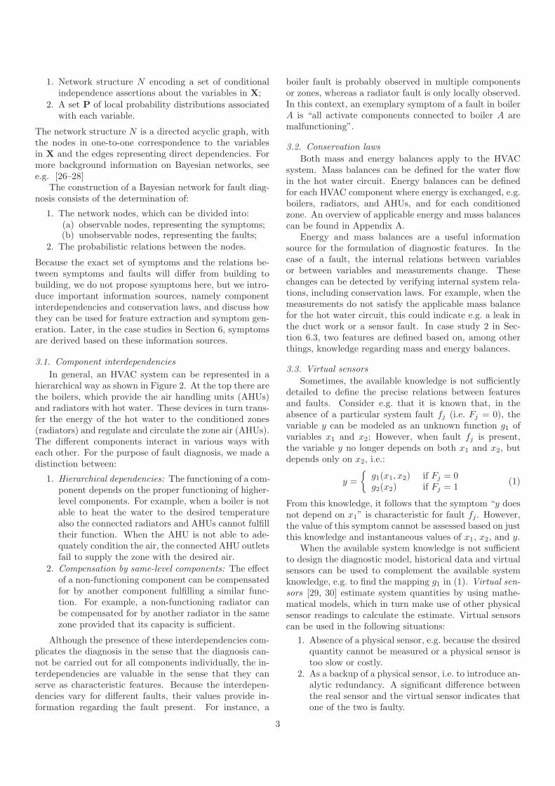
3.1. Component interdependencies

In general, an HVAC system can be represented in ahierarchical way as shown in Figure 2. At the top there arethe boilers, which provide the air handling units (AHUs)and radiators with hot water. These devices in turn trans-fer the energy of the hot water to the conditioned zones(radiators) and regulate and circulate the zone air (AHUs).The different components interact in various ways witheach other. For the purpose of fault diagnosis, we made adistinction between:

1. Hierarchical dependencies: The functioning of a com-ponent depends on the proper functioning of higher-level components. For example, when a boiler is notable to heat the water to the desired temperaturealso the connected radiators and AHUs cannot fulfilltheir function. When the AHU is not able to ade-quately condition the air, the connected AHU outletsfail to supply the zone with the desired air.

2. Compensation by same-level components: The effectof a non-functioning component can be compensatedfor by another component fulfilling a similar func-tion. For example, a non-functioning radiator canbe compensated for by another radiator in the samezone provided that its capacity is sufficient.

Although the presence of these interdependencies com-plicates the diagnosis in the sense that the diagnosis can-not be carried out for all components individually, the in-terdependencies are valuable in the sense that they canserve as characteristic features. Because the interdepen-dencies vary for different faults, their values provide in-formation regarding the fault present. For instance, a

boiler fault is probably observed in multiple componentsor zones, whereas a radiator fault is only locally observed.In this context, an exemplary symptom of a fault in boilerA is “all activate components connected to boiler A aremalfunctioning”.

3.2. Conservation laws

Both mass and energy balances apply to the HVACsystem. Mass balances can be defined for the water flowin the hot water circuit. Energy balances can be definedfor each HVAC component where energy is exchanged, e.g.boilers, radiators, and AHUs, and for each conditionedzone. An overview of applicable energy and mass balancescan be found in Appendix A.

Energy and mass balances are a useful informationsource for the formulation of diagnostic features. In thecase of a fault, the internal relations between variablesor between variables and measurements change. Thesechanges can be detected by verifying internal system rela-tions, including conservation laws. For example, when themeasurements do not satisfy the applicable mass balancefor the hot water circuit, this could indicate e.g. a leak inthe duct work or a sensor fault. In case study 2 in Sec-tion 6.3, two features are defined based on, among otherthings, knowledge regarding mass and energy balances.

3.3. Virtual sensors

Sometimes, the available knowledge is not sufficientlydetailed to define the precise relations between featuresand faults. Consider e.g. that it is known that, in theabsence of a particular system fault fj (i.e. Fj = 0), thevariable y can be modeled as an unknown function g1 ofvariables x1 and x2; However, when fault fj is present,the variable y no longer depends on both x1 and x2, butdepends only on x2, i.e.:

y =

{

g1(x1, x2) if Fj = 0g2(x2) if Fj = 1

(1)

From this knowledge, it follows that the symptom “y doesnot depend on x1” is characteristic for fault fj . However,the value of this symptom cannot be assessed based on justthis knowledge and instantaneous values of x1, x2, and y.

When the available system knowledge is not sufficientto design the diagnostic model, historical data and virtualsensors can be used to complement the available systemknowledge, e.g. to find the mapping g1 in (1). Virtual sen-sors [29, 30] estimate system quantities by using mathe-matical models, which in turn make use of other physicalsensor readings to calculate the estimate. Virtual sensorscan be used in the following situations:

1. Absence of a physical sensor, e.g. because the desiredquantity cannot be measured or a physical sensor istoo slow or costly.

2. As a backup of a physical sensor, i.e. to introduce an-alytic redundancy. A significant difference betweenthe real sensor and the virtual sensor indicates thatone of the two is faulty.

3

central equipment

intermediate equipment

terminal equipment

conditioned building

wall 1 wall i

boiler 1 boiler j

AHU 1 AHU k

outlet 1 outlet l radiator 1 radiator m

zone 1 zone 2 zone n

Figure 2: An illustration of the (hierarchical) dependencies among the HVAC components in a building.

3. To estimate the behavior of a system variable corre-sponding to a specific type of system behavior, e.g.healthy behavior. In this case, the virtual sensor istrained using data corresponding to the consideredsystem behavior and a significant difference betweenthe actual sensor reading and the virtual sensor out-put indicates that the system does not behave ac-cording to the considered behavior.

In the case studies in Section 6, a virtual sensor coveringsituation 3 is constructed and in Section 7, examples areprovided where situation 1 applies.

The design of a virtual sensor essentially consists ofthree steps:

Step 1: The choice for the quantity to be estimated, i.e.which variables are valuable features for diagnosis.

Step 2: The selection of available sensor measurements thatare relevant to estimate these quantities

Step 3: The choice for the method to capture the relationbetween the quantity of interest and the relevantsensor measurements, e.g. first principles or data-based approaches.

In this work, the main focus is on the first two steps. Forthe third step, a standard data-based approach from liter-ature, nearest neighbor regression [31], can be used.

4. Fault diagnosis strategy

4.1. Construction of the diagnostic model

Procedure 1 describes the construction of the diagnos-tic model, in the form of a set of Bayesian networks. In line1, the system faults f1 till fn are determined, e.g. basedon expert knowledge. Next, in lines 2 − 4, a binary nodeFi is assigned to each system fault fi. Note that a binarynode is used for each of the faults to easily handle multiplefault scenarios. Next, in line 5, an appropriate symptomset is determined based on knowledge and data regard-ing component interdependencies and conservation laws.

Subsequently, a node Sj is assigned to each of the symp-toms (lines 6−8). Next, the different operating modes aredetermined (line 9). For each of them, the relationshipsbetween the system faults and the symptoms are defined(i.e. the corresponding network is built) (lines 11− 13).

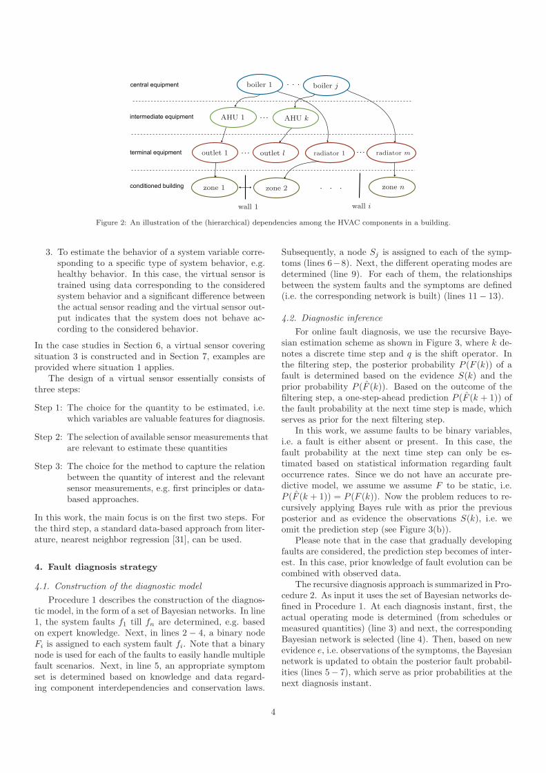
4.2. Diagnostic inference

For online fault diagnosis, we use the recursive Baye-sian estimation scheme as shown in Figure 3, where k de-notes a discrete time step and q is the shift operator. Inthe filtering step, the posterior probability P (F (k)) of afault is determined based on the evidence S(k) and theprior probability P (F (k)). Based on the outcome of thefiltering step, a one-step-ahead prediction P (F (k + 1)) ofthe fault probability at the next time step is made, whichserves as prior for the next filtering step.

In this work, we assume faults to be binary variables,i.e. a fault is either absent or present. In this case, thefault probability at the next time step can only be es-timated based on statistical information regarding faultoccurrence rates. Since we do not have an accurate pre-dictive model, we assume we assume F to be static, i.e.P (F (k + 1)) = P (F (k)). Now the problem reduces to re-cursively applying Bayes rule with as prior the previousposterior and as evidence the observations S(k), i.e. weomit the prediction step (see Figure 3(b)).

Please note that in the case that gradually developingfaults are considered, the prediction step becomes of inter-est. In this case, prior knowledge of fault evolution can becombined with observed data.

The recursive diagnosis approach is summarized in Pro-cedure 2. As input it uses the set of Bayesian networks de-fined in Procedure 1. At each diagnosis instant, first, theactual operating mode is determined (from schedules ormeasured quantities) (line 3) and next, the correspondingBayesian network is selected (line 4). Then, based on newevidence e, i.e. observations of the symptoms, the Bayesiannetwork is updated to obtain the posterior fault probabil-ities (lines 5− 7), which serve as prior probabilities at thenext diagnosis instant.

4

(a) (b)

S(k)S(k) filteringfiltering

P(

F (k + 1))

=P (F (k))

P (F (k))

P(

F (k + 1)) q−1q−1

prediction

prior = P(

F (k))prior = P

(

F (k))

Figure 3: Bayesian fault diagnosis scheme, with evidence S(k) the observations at time k, F (k) the fault variable at time k, and q the shiftoperator: (a) the full scheme; (b) the simplified scheme adopted in this paper.

Procedure 1 Model constructionInput: Expert knowledge, historical data1: Determine possible system faults f1 till fn2: for i = 1, ..., n do

3: Define binary node Fi

4: end for

5: Determine symptoms S1 till Sm based on expert knowledgeand data

6: for j = 1, ...,m do

7: Define discrete-valued node Sj

8: end for

9: Determine the system’s operating modes 1 till ℓ10: for h = 1, ..., ℓ do

11: Determine Nh, which is the network structure definingthe relations between the symptoms S1 till Sm and thefault variables F1 till Fn, in operating mode h

12: Determine Ph, which is the set of local probability func-tions associated with each node in Nh

13: end for

Output: Bayesian network (Nh,Ph) for each operatingmode h

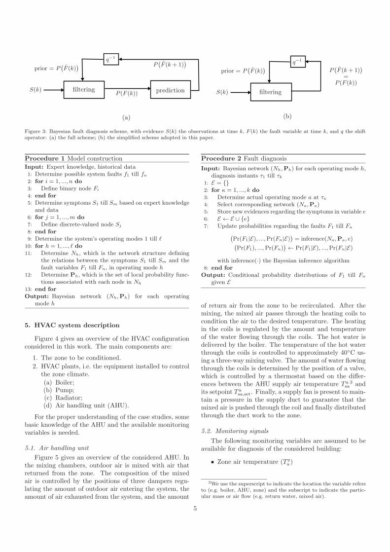
5. HVAC system description

Figure 4 gives an overview of the HVAC configurationconsidered in this work. The main components are:

1. The zone to be conditioned.

2. HVAC plants, i.e. the equipment installed to controlthe zone climate.

(a) Boiler;(b) Pump;(c) Radiator;(d) Air handling unit (AHU).

For the proper understanding of the case studies, somebasic knowledge of the AHU and the available monitoringvariables is needed.

5.1. Air handling unit

Figure 5 gives an overview of the considered AHU. Inthe mixing chambers, outdoor air is mixed with air thatreturned from the zone. The composition of the mixedair is controlled by the positions of three dampers regu-lating the amount of outdoor air entering the system, theamount of air exhausted from the system, and the amount

Procedure 2 Fault diagnosis

Input: Bayesian network (Nh,Ph) for each operating mode h,diagnosis instants τ1 till τk

1: E = {}2: for κ = 1, ..., k do

3: Determine actual operating mode a at τκ4: Select corresponding network (Na,Pa)5: Store new evidences regarding the symptoms in variable e6: E ← E ∪ {e}7: Update probabilities regarding the faults F1 till Fn

(

Pr(F1|E), ...,Pr(Fn|E))

= inference(Na,Pa, e)(

Pr(F1), ...,Pr(Fn))

← Pr(F1|E), ...,Pr(Fn|E)

with inference(·) the Bayesian inference algorithm8: end for

Output: Conditional probability distributions of F1 till Fn

given E

of return air from the zone to be recirculated. After themixing, the mixed air passes through the heating coils tocondition the air to the desired temperature. The heatingin the coils is regulated by the amount and temperatureof the water flowing through the coils. The hot water isdelivered by the boiler. The temperature of the hot waterthrough the coils is controlled to approximately 40◦C us-ing a three-way mixing valve. The amount of water flowingthrough the coils is determined by the position of a valve,which is controlled by a thermostat based on the differ-ences between the AHU supply air temperature T a

sa3 and

its setpoint T asa,set. Finally, a supply fan is present to main-

tain a pressure in the supply duct to guarantee that themixed air is pushed through the coil and finally distributedthrough the duct work to the zone.

5.2. Monitoring signals

The following monitoring variables are assumed to beavailable for diagnosis of the considered building:

• Zone air temperature (T za )

3We use the superscript to indicate the location the variable refersto (e.g. boiler, AHU, zone) and the subscript to indicate the partic-ular mass or air flow (e.g. return water, mixed air).

5

Radiator

Zone

thermostat

temperature

sensor

A��

outlet s�����

air

s����� ���

radiator

temperature

sensorthermostat

boilers����� ���

boiler

��

P���

return ���

radiator

return ���

boiler

s����� ���

��

z��

air

return ����

���

outside

air

T bsw,set T z

a,set

T asa,set

T za

T asa

Figure 4: Overview of the considered HVAC system. Dotted lines represent air flows, dashed lines represent mass flows, and solid linesrepresent signals.

T asa,set

outside air

exhaust air

mixed air supply air

zone

zone air

Ua

supply water

return water

heating coils

T asa

thermostat

sensor

damper settings

fan speed

Figure 5: Schematic overview of an AHU.

6

• Supply air temperature (T asa)

• Mixed air temperature (T ama)

• Outside air temperature (T oa )

• Supply water temperature (T bsw)

• Return water temperature (T brw)

• Mass flow through the boiler (wbsw)

• Control signal to AHU valve (Ua)

• Control signal to the radiator valve (U r)

Furthermore, the zone air temperature setpoint (T za,set),

supply air temperature setpoint (T asa,set), and supply water

temperature setpoint (T bsw,set) are assumed to be known.

6. Fault diagnosis case studies

In this section, the proposed method is illustrated basedon two case studies. Case study 1 comprises the fault de-tection of a stuck AHU heating coil valve and mainly servesto illustrate the problems that occur when neglecting thedifferent operating modes and interdependencies betweenHVAC components. Case study 2 extends case study 1 inthe sense that the possibility of a non-functioning boileris included. Although this case study is still relativelysimple, it clearly illustrates the implications of multipleoperation modes and component interdependencies on thefault diagnosis, and how they are handled in the proposeddiagnosis approach.

6.1. Simulation model

6.1.1. System modeling

For the purpose of analysis and validation, experts atHoneywell have developed a simulation model of the con-sidered building [32]. The model has been verified usingdata obtained from real buildings. The model makes a dis-tinction between two sets of variables: temperatures andmass flows. As the pressure dynamics are much faster thanthe temperature dynamics, the transient behavior of themass flow rates is neglected, i.e.:

wasw(t) = fa (X

a(t), Xr(t)) (2)

wrsw(t) = fr (X

a(t), Xr(t)) (3)

with wasw and wr

sw the mass flows through the AHU andradiator respectively, and Xa and Xr the positions of theAHU valve and the radiator valve. For more details on thesimulation model, see [32].

6.1.2. Fault modeling

Stuck heating coil valve. A stuck valve stays in the posi-tion it was before it got stuck, regardless of the controlsignal Ua sent to the valve by the thermostat. This meansthat the mass flow through the heating coil remains thesame. In the simulation model, a stuck valve is modeledby constraining the mass flow to be constant, i.e.:

wasw(t) = wa

sw(ta) ∀t ≥ ta (4)

with ta the time that the valve stopped functioning.

Non-functioning boiler. When the boiler breaks down, thewater returning from the hot water circuit is no longerheated to the supply water temperature setpoint T b

sw,set,

i.e. the supply water temperature T bsw becomes equal to

the return water temperature T brw. Therefore, a non-func-

tioning boiler is modeled as follows4:

T bsw(t) = T b

rw(tb) ∀t ≥ tb (5)

with tb the time that the boiler stopped functioning.

6.1.3. Simulation specifications

1. The daily schedule is defined as:

• day operation between 04.00 and 18.00 hours;

• night operation between 18.00 and 04.00 hours.

2. The setpoints of the boiler supply water temperatureT bsw, the AHU supply air temperature T a

sa, and thezone air temperature T z

a are:

T bsw,set =

{

75 day operation65 night operation

T asa,set =

{

20 day operation- night operation

T za,set =

{

21 day operation18 night operation

3. Damper positions are fixed, i.e. the ratio betweenzone air and outside air is constant (1:4 during theday and 3:7 during the night).

4. Fan speed is fixed, i.e. wasa is constant (0.1kg/s during

the day and 0.001kg/s during the night).

5. Detailed weather reports of the winter season areavailable as input for the simulation.

6.2. Case study 1

Consider the building configuration depicted in Fig-ure 4 and assume that the system is healthy except fora possibly stuck AHU heating coil valve. Our aim is todetermine whether or not the valve is stuck. This is achallenging problem because:

4Note that in practice there is some delay between the time theboiler stops functioning and the time the supply water temperaturebecomes equal to the temperature of the return water. We assumethis delay to be small and neglect it in the remainder.

7

F a

S1 T ama

(a) AHU on

F a

S1 T ama

(b) AHU off

Figure 6: Bayesian network representations of case study 1. Duringday symptom S1 is influenced by both an AHU fault and by themixed air temperature. During night, the AHU is switched off andthe relations between F a, T a

ma, and S1 no longer hold.

1. The extent to which the fault expresses itself in themeasured variables highly depends on the position inwhich the valve got stuck and on weather conditions;

2. The mass flow through the valve is not measured.

6.2.1. Diagnostic model

Network structure. Given the measurements specified inSection 5.2, an obvious way to detect a stuck heating coilvalve is to compare the supply air temperature T a

sa withits setpoint T a

sa,set. In the case of a broken valve, a dif-ference between the two temperatures is expected. Thisknowledge gives rise to define symptom S1 as:

S1 =

{

1 if |T asa − T a

sa,set| > ǫ10 otherwise

(6)

with ǫ1 > 0 a user-defined threshold. The system healthis related to symptom S1 as follows:

If the system is healthy, i.e. F a = 0 then likely S1 = 0

If the valve is broken, i.e. F a = 1 then likely S1 = 1

with F a a binary variable indicating whether the AHUvalve is healthy (F a = 0) or stuck (F a = 1). Here,“likely” indicates that due to uncertain influences, we arenot completely sure about the relations. The degree of un-certainty is expressed in the conditional probability tableof S1, which will be defined later. The relations hold underthe assumptions that the system operates in day mode andT ama ≤ T a

sa,set. Because the supply air temperature T asa is

not controlled during the night, a stuck heating coil valveis only expressed in symptom S1 during the day. Further-more, as only heating is present in the considered system,in the summer period when T a

ma > T asa,set, too high a value

of the supply air temperature can be both due to a stuckvalve or due to high outside temperatures.

The proposed diagnostic model is graphically repre-sented by the Bayesian networks in Figure 6. Due to theimposed day and night schedule, the system must oper-ate in two modes, which are also reflected in the diagnos-tic model. As the available simulation data concern thewinter season, in which case T a

ma < T asa,set, node T a

ma isneglected in the remainder.

0 10 20 30 40 50 60

6

8

10

12

14

16

18

20

22

24

Supply

air

tem

perature

Ta sa

(◦C)

Time (hours)

Figure 7: Daily behavior of the supply air temperature. Note thatduring the night, the AHU supply air temperature is not controlled.

Local probability distributions. To complete the construc-tion of the Bayesian network, the following items need tobe determined:

1. the value of ǫ1;

2. the conditional probability table of S1;

3. the initial prior probability distribution of F a.

Determination of ǫ1 To determine ǫ1, the nomi-nal variations in T a

sa are considered. Figure 7 shows thebehavior of T a

sa on three consecutive days. It can be ob-served that in the morning, when the system switches today mode, it takes some time (about half an hour) beforethe supply air temperature has converged to its desiredvalue T a

sa,set = 20◦C. After this time, the temperaturefluctuates around its desired value. To gain some insightinto the degree of fluctuation, in Figure 8 the histogram of|T a

sa − T asa,set| containing data of two consecutive months

is shown. We tune the value of ǫ1 such that 99% of theT asa values between 04.30 and 18.00 hours are within the

interval [T asa,set − ǫ1, T

asa,set + ǫ1], resulting in

ǫ1 = 2.5

Conditional probability table of S1 As ǫ1 is tunedsuch that in 99% of the healthy cases it holds that S1 = 0,the probability that S1 = 1 given the system is healthyis 1%. To determine the probability that S1 = 1 given astuck heating coil valve, simulation data from faulty be-havior are considered5. Actually, the data set used for thismust contain measurements corresponding to faults in alldifferent valve positions and for all relevant weather con-ditions. Figure 9 shows two completely different behaviors

5Instead of using (simulation) data, these probabilities can alsobe directly derived from expert knowledge.

8

0 0.5 1 1.5 2 2.5 3 3.5 40

2000

4000

6000

8000

10000

12000

14000

16000

Deviation from setpoint °C

Num

ber

of occure

nce

Figure 8: Distribution of |T asa − T a

sa,set|.

Table 1: Conditional probability table of S1, the values correspond-ing to P (S1|F a)

S1

F a 0 1

0 0.99 0.011 0.24 0.76

of T asa corresponding to a stuck AHU valve. In the first sit-

uation, the valve got stuck during night in a cold period,whereas in the second situation, the valve got stuck duringday while the outside temperature is increasing. Here, theprobability of S1 = 1 given an AHU valve fault (F a = 1) isapproximated based on a finite number of randomly cho-sen fault scenarios. The results are included in Table 1.

Initial prior probability distribution of F a Inthe first diagnosis step, a user-defined prior Pr0(F a = 1) =0.01 is used. The initial prior probability Pr0(F a = 1)indicates how likely we consider the occurrence of an AHUvalve fault before observing the monitoring data. Notethat from Bayes’ rule, which state that:

Pr(F a|S1) =Pr(S1|F

a) Pr(F a)∑

y∈ΘFaPr(S1|y) Pr(y)

(7)

with ΘF a = {0, 1} the domain of F a

it follows that the influence of the initial prior probabilitydistribution on the fault diagnosis is small as the proba-bilities are recursively updated every minute and the like-lihood functions have clearly different values for F a = 0and F a = 1 (see Table 1).

6.2.2. Fault diagnosis

The proposed approach is demonstrated by means oftwo simulations. In the first example (see Figure 10), thevalve got stuck in a cold period during the night (aroundtime t = 220 hours). As a consequence, the air in the AHUis not sufficiently heated during the subsequent day, symp-tom S1 becomes equal to one, and shortly afterwards, anAHU fault is detected, i.e. F a = Pr(F a = 1|E) ≈ 1, where,because of the recursive nature of the Bayesian approach,E contains all observations of symptom S1. Besides thecorrect fault detection around t = 220 hours, an AHUfault is incorrectly detected around t = 160 hours. Thisincorrect detection is of a very short duration and a conse-quence of the way ǫ1 is tuned. Recall that ǫ1 is tuned suchthat in 1% of the healthy cases symptom S1 is activated. Ifthis happens at several consecutive time instants, this willlead to a false positive detection6. In the second example(see Figure 11), the valve got stuck during the day. As theposition in which the valve got stuck was quite favorablewith respect to the supply air temperature setpoint in thesubsequent days, the fault is only detected after four days,i.e. as soon as the effects become observable.

6.2.3. Concluding remarks

Although the diagnostic model defined in Section 6.2.1turned out to be effective in the sense that in the sim-ulations faults are detected as soon as their effects areobservable, diagnosis is not carried out continuously in alloperating modes. Specific shortcomings are:

1. Faults cannot be detected during the night;

2. The model is not useful for high mixed-air tempera-tures;

3. The underlying assumptions are too simplistic, e.g.as only an AHU valve fault is allowed, hierarchicalrelationships are assumed to be absent.

Therefore, the next section deals with a case study includ-ing multiple fault scenarios where the goal is to determinea diagnostic model that it is less sensitive to high valuesof the mixed air temperature and that allows for fault di-agnosis in all operating modes.

6.3. Case study 2

This case study extends the problem discussed in Sec-tion 6.2 by including the possibility of a non-functioningboiler. In this case, there are four possible fault scenarios:

1. Healthy system;

2. Stuck heating coil valve:

3. Non-functioning boiler;

4. Both the valve and the boiler are non-functioning.

6Remember that we consider a recursive filter in which the posterprobabilities serve as prior at the next time step.

9

0 100 200 300 400 500 600 700 800 900 1000-10

0

10

20

0 100 200 300 400 500 600 700 800 900 1000-20

0

20

Time (hours)

0 100 200 300 400 500 600 700 800 900 1000-0.5

0

0.5

1

1.5

Ta sa

To a

Fa

0 100 200 300 400 500 600 700 800 900 100010

20

30

0 100 200 300 400 500 600 700 800 900 1000

-10

0

10

20

30

Time (hours)

0 100 200 300 400 500 600 700 800 900 1000-0.5

0

0.5

1

1.5

Ta sa

To a

Fa

Figure 9: Possible behaviors of T asa corresponding to a stuck heating coil valve. Left: the valve got stuck during the night in a cold period.

Right: the valve got stuck during the day while the outside temperature is increasing.

0 50 100 150 200 2500

10

20

30

0 50 100 150 200 250

0

0.5

1

Time (hours)

0 50 100 150 200 250

0

0.5

1fault

fault estimation

Ta sa

S1

Fa,F

a

Figure 10: AHU fault diagnosis example 1.

0 50 100 150 200 250 3000

10

20

30

0 50 100 150 200 250

0

0.5

1

Time (hours)

0 50 100 150 200 250

0

0.5

1fault

fault estimation

Ta sa

S1

Fa,F

a

Figure 11: AHU fault diagnosis example 2.

6.3.1. Diagnostic model

Network structure. Besides that the diagnostic model forcase study 1 does not support fault diagnosis during thenight and is sensitive to high values of the mixed air tem-perature, the model cannot distinguish between all faultscenarios. If S1 = 1 all scenarios except for scenario 1 areplausible. To make a further distinction between the differ-ent fault scenarios possible, symptom S1 is extended froma binary valued symptom to a three-valued symptom S′

1:

S′

1 =

−1 if (T asa − T a

sa,set) ∈ (−∞,−ǫ1)0 if (T a

sa − T asa,set) ∈ [−ǫ1, ǫ1]

1 otherwise(8)

Symptom S′

1 relates to the system health as follows:

If F a = F b = 0 then likely S′

1 = 0

If F a = 1 and F b = 0 then likely S′

1 = −1 or S′

1 = 1

If F b = 1 then likely S′

1 = −1

So, S′

1 = 0 characterizes a healthy system and S′

1 = 1characterizes an AHU valve that got stuck in a too openedposition. When S′

1 = −1, scenarios 2, 3, and 4 are all pos-sible. To improve the diagnostic power and to allow fordiagnosis during both the day and the night, two addi-tional symptoms are proposed: S2 to the verify the properfunctioning of the AHU valve and S3 to verify the properfunctioning of the boiler.

To verify whether or not the valve is stuck, the rela-tionships between the mass flow through the boiler wb

sw

and the control signals Ua and U r to the AHU valve andthe radiator valve respectively are used:

• When F a = 0, the mass flow through the boiler wbsw

depends both on the control signal to the AHU valveUa and the control signal to the radiator valve U r.

• When F a = 1, the mass flow through the boiler wbsw

no longer depends on Ua, but depends only on U r.

10

F a F b

S′

1 S2 S3

T ama

(a) AHU on

F a F b

S′

1 S2 S3

T ama

(b) AHU off

Figure 12: Bayesian network representations of case study 2. Duringday, symptom S′

1is influenced by both F a, Fb, and T a

ma, symptomS2 is influenced by F a, and symptom S3 is influenced by Fb. Duringnight, when the AHU is switched off, only the relations between F a

and S2 and between Fb and S3 still hold.

This follows from the applicable mass balance (A.1) andequations (2) and (3). Since the relationships among wb

sw, Ua,

and U r are not exactly known, we construct a virtual sen-sor that predicts the mass flow through the boiler wb

sw

based on the AHU and radiator valve control signals Ua

and U r. The virtual sensor is trained based on healthydata. So, the virtual sensor estimate wb

sw(Ua, U r) will be

close to its actual value wbsw when the AHU valve functions

properly. When the AHU valve is broken, the virtual sen-sor estimate wb

sw(Ua, U r) likely differs from the measured

value wbsw. This gives symptom S2 as:

S2 =

{

1 if |wbsw − wb

sw(Ua, U r)| > ǫ2

0 otherwise(9)

Symptom S2 is linked to the system health as follows:

If F a = 0 then likely S2 = 0

If F a = 1 then likely S2 = 1

To verify whether the boiler is functioning, a straight-forward approach is to compare the boiler supply watertemperature T b

sw with its setpoint T bsw,set. In case of boiler

non-functioning these two values will differ significantly.To this end, symptom S3 is defined as:

S3 =

{

0 if (T bsw − T b

sw,set) ∈ [−ǫ3,∞)1 otherwise

(10)

with ǫ3 > 0, which links to the system health as follows:

If F b = 0 then likely S3 = 0

If F b = 1 then likely S3 = 1

Considering the symptoms S′

1, S2, and S3, the diagnosticmodel for this case is represented by the Bayesian networkin Figure 12. A distinction is made between two operatingmodes: a day mode (AHU on) and a night mode (AHUoff). Fault diagnosis can be carried out in both modes.

Similarly as for case study 1, we restrict ourselves todiagnosis in the cold season, i.e. node T a

ma is disregarded.

Time (hours)

0 200 400 600 800 1000 1200

×10-3

-8

-6

-4

-2

0

2

4

6

8

10

wb sw−

wb sw

(a) F a = 0

Time (hours)

0 200 400 600 800 1000 1200-0.03

-0.02

-0.01

0

0.01

0.02

0.03

0.04

0.05

wb sw−

wb sw

(b) F a = 1

Figure 13: Time behavior of wbsw − wb

sw.

Local probability distributions. Before the network can beused for diagnostic inference, the following items need tobe determined:

1. the values of ǫ1, ǫ2, and ǫ3

2. the conditional probability tables of S′

1, S2, and S3

3. the initial prior probability distributions of F a andF b

Determination of ǫ1, ǫ2, and ǫ3 The value of ǫ1 ischosen similar as in case study 1 (as the variation of wa

sa

is symmetrical around 20◦C, there is no need to make adistinction between positive and negative deviations), i.e.

ǫ1 = 2.5

To determine ǫ2, the variation in wbsw −wb

sw is considered.In Figure 13, time behaviors of wb

sw−wbsw are given for both

a healthy and a stuck AHU valve. The value of ǫ2 is chosensuch that given F a = 0, it holds that Pr(S2 = 0) = 0.99.This is the case for

ǫ2 = 0.003

Finally, ǫ3 is tuned. As the boiler supply water tempera-ture setpoint T b

sw,set changes at 04.00 hours in the morningand at 18.00 hours in the evening, there is some natu-ral difference between T b

sw and T bsw,set shortly after these

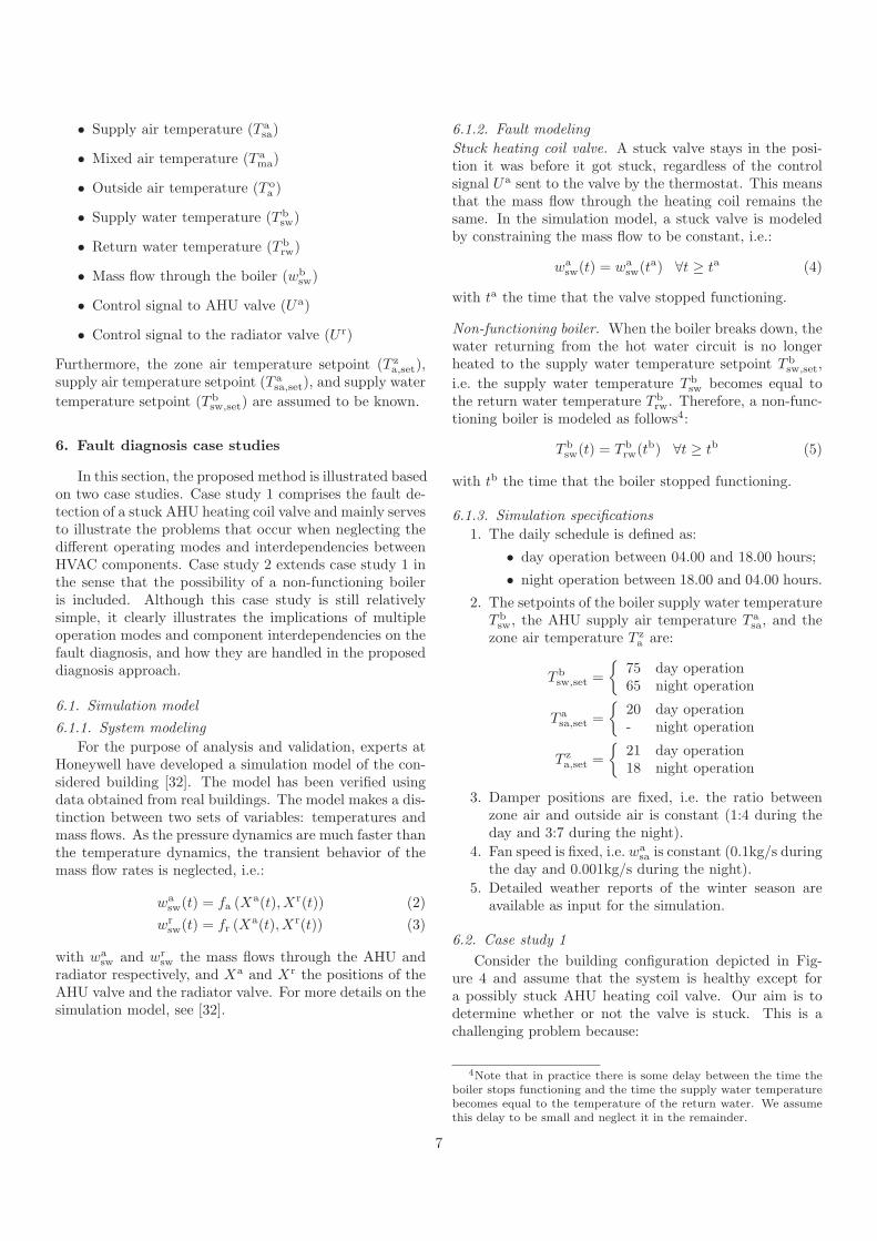
times (see Figure 14). Therefore, for fault diagnosis andthe determination of ǫ3, only the time intervals 04.30 till18.00 hours and 18.30 till 04.00 hours are considered. Thevalue of ǫ3 is chosen such that given F b = 0, it holds thatPr(S3 = 0) = 0.99, i.e.:

ǫ3 = 0.8

Conditional probability tables of S′

1, S2, and S3

The conditional probability tables are defined similarly asin case study 1. The results are given in Tables 2 till 4.

7If the boiler is broken the temperature significantly decreasesand if the fault holds for some time this probability converges toone.

11

Time (hours)

0 5 10 15 20 25

64

66

68

70

72

74

76

Tb sw

Tbsw

Tbsw,set

Figure 14: Daily behavior of Tbsw.

Table 2: Conditional probability table of S′

1

S1

F a F b -1 0 1

0 0 0.05 0.99 0.051 0 0.47 0.24 0.280 1 17 0 01 1 1 0 0

Table 3: Conditional probability table of S2

S2

F a 0 1

0 0.99 0.011 0.11 0.89

Table 4: Conditional probability table of S3

S3

F b 0 1

0 0.99 0.011 0 1

0 50 100 150 200 250

-1

0

1

0 50 100 150 200 250

0

0.5

1

Time (hours)

0 50 100 150 200 250

0

0.5

1

S′ 1,S2,S3

Fa,F

aF

b,F

b

S′

1S2S3

F a

F a

Fb

Fb

Figure 15: Boiler and AHU fault diagnosis example.

Prior probability distributions of F a and F b Theinitial prior probability distributions are defined similarlyas for case study 1:

Pr0(F a = 1) = Pr0(F b = 1) = 0.01

Again the effect of the initial priors on the fault diagnosisis small as the likelihood functions have clearly differentvalues for the different fault situations (see Tables 2, 3,and 4).

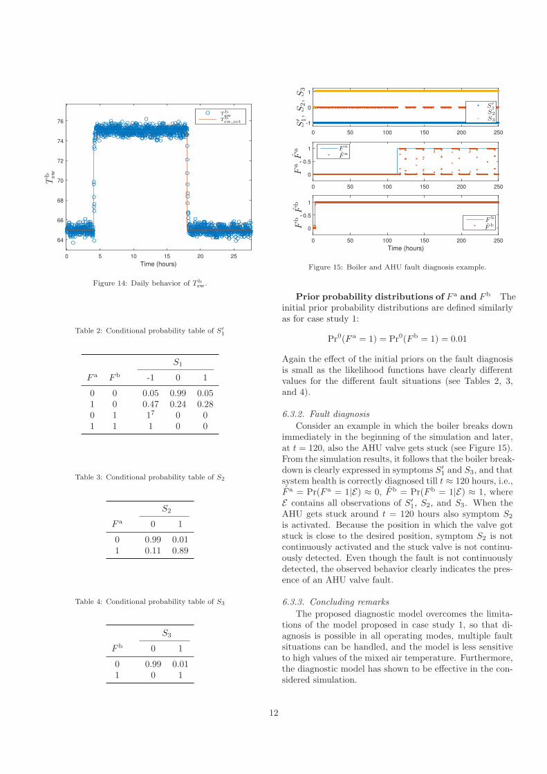
6.3.2. Fault diagnosis

Consider an example in which the boiler breaks downimmediately in the beginning of the simulation and later,at t = 120, also the AHU valve gets stuck (see Figure 15).From the simulation results, it follows that the boiler break-down is clearly expressed in symptoms S′

1 and S3, and thatsystem health is correctly diagnosed till t ≈ 120 hours, i.e.,F a = Pr(F a = 1|E) ≈ 0, F b = Pr(F b = 1|E) ≈ 1, whereE contains all observations of S′

1, S2, and S3. When theAHU gets stuck around t = 120 hours also symptom S2

is activated. Because the position in which the valve gotstuck is close to the desired position, symptom S2 is notcontinuously activated and the stuck valve is not continu-ously detected. Even though the fault is not continuouslydetected, the observed behavior clearly indicates the pres-ence of an AHU valve fault.

6.3.3. Concluding remarks

The proposed diagnostic model overcomes the limita-tions of the model proposed in case study 1, so that di-agnosis is possible in all operating modes, multiple faultsituations can be handled, and the model is less sensitiveto high values of the mixed air temperature. Furthermore,the diagnostic model has shown to be effective in the con-sidered simulation.

12

6.4. Alternative symptoms for case study 2

Although the diagnostic model for case study 2 resultsin good performance, there may exist situations in whichother or additional symptoms are required (e.g. in caseof an absent or broken supply water temperature sensor).Therefore, we conclude this section with the proposal oftwo alternative symptoms for case study 2:

1. Find and use the relationship between the supply airtemperature T a

sa, the mixed air temperature T ama, the

supply water temperature T bsw, and the control sig-

nal to the AHU valve Ua. Depending on the actualsystem health, the AHU supply air temperature T a

sa

can be described as a function of:

T ama, U

a if F a = F b = 0T ama if F a = 1, F b = 0

T ama, U

a, T bsw if F a = 0, F b = 1

T ama, T

bsw if F a = 1, F b = 1

(11)

These relations follow from the energy balance (A.4),the knowledge that the thermal energy of air/waterdepends on its temperature and volume, and the factthat, for a healthy valve, the mass flow wa

sw is directlyrelated to the control signal Ua. Since the exact re-lationships are unknown, we use this knowledge toconstruct two virtual sensors. Multiple virtual sen-sors are needed since in this case, a distinction be-tween multiple scenarios has to be made8. For ex-ample, one virtual sensor T a

sa(Tama, U

a) is designed toestimate the AHU supply air temperature T a

sa corre-sponding to healthy system behavior (F a = F b = 0)and another one T a

sa(Tama, U

a, T bsw) to estimate the

behavior of T asa corresponding to a non-functioning

boiler (F a = 0, F b = 1). Accordingly, symptom Sa1

is defined as (12) and linked to the system health asfollows:

• If F a = F b = 0 then likely Sa1 = 0

• If F a = 0 and F b = 1 then likely Sa1 = −1

• If F a = 1 then likely Sa1 = 1

A possible drawback of this symptom is that it relieson the availability of historical data of fault situa-tions for designing the virtual sensor (in this casehistorical data of a non-functioning boiler). How-ever, when a good physical simulator is available,simulated data can also be used to train the virtualsensor.

2. Verify whether other AHUs or radiators connectedto the same boiler function properly. This strategycan be used provided that multiple systems (e.g. ra-diators and AHUs) are connected to the same boiler.In case of a boiler fault, also the connected systems

8For sake of clarity, we restrict ourselves to two virtual sensorshere.

will exhibit aberrant behavior (hierarchical depen-dencies, see Section 3.1). In the considered buildingconfiguration, one radiator is connected to the sameboiler as the considered AHU. If this radiator func-tions properly this indicates that the boiler cannot bebroken (provided that radiator heating is required).This knowledge gives rise to defining symptom Sa2

as:

Sa2 =

{

1 if T za − T z

a,set < ǫa20 otherwise

(13)

which is linked to the system health as follows:

If F b = 0 then likely Sa2 = 0

If F b = 1 then likely Sa2 = 1

Note that it is assumed that the radiator functionsproperly and that this symptom is only useful whenradiator heating is required.

Taking the additional symptoms Sa1 and Sa2 into accountthe diagnostic model is represented by the Bayesian net-work in Figure 16. Now, a distinction between four oper-ating modes has to be made. An advantage of this modelcompared to the original model (see Figure 12) is that, dueto its redundancy, fault diagnosis is also possible when oneof the symptoms is missing. In addition, the redundancycan be used to detect possible sensor faults.

7. Discussion on generalization

So far, the focus was on one particular HVAC configu-ration. In practice, each building is different, e.g. it mayhave another number of zones, different types of separa-tion between the zones, and different HVAC equipmentinstalled to condition the building. Therefore, it is impor-tant to consider how the diagnostic model can be extendedto other cases.

7.1. Different HVAC equipment

In general, a building (including HVAC system) can berepresented as shown in Figure 2. The number of compo-nents in each layer and the way the components are con-nected varies from building to building. These differencesinfluence the diagnostic model. Here, it is shown that evenfor two slightly different HVAC configurations the diag-nostic model may vary. For this purpose, an additionalradiator is installed in the building setup considered be-fore (Figure 2). In the original building, a non-functioningradiator, F r = 1, will manifest itself in a too low zonetemperature (provided that radiator heating is required).This gives rise to use symptom Sg1 , which is defined as:

Sg1 =

{

1 if T za − T z

a,set < −ǫg10 otherwise

(14)

and linked to the system health as:

If F r = 0 then likely Sg1 = 0

13

Sa1 =

−1 if∣

∣T asa − T a

sa(Tama, U

a, T bsw)

∣

∣ < ǫa1 and∣

∣T asa − T a

sa(Tama, U

a, T bsw)

∣

∣ ≤∣

∣T asa − T a

sa(Tama, U

a)∣

∣

0 if∣

∣T asa − T a

sa(Tama, U

a)∣

∣ < ǫa1 and∣

∣T asa − T a

sa(Tama, U

a, T bsw)

∣

∣ >∣

∣T asa − T a

sa(Tama, U

a)∣

∣

1 otherwise

(12)

F a F b

S′

1 S2 S3Sa1 Sa2

T ama

(a) AHU on, Radiator on

F a F b

S′

1 S2 S3Sa1 Sa2

T ama

(b) AHU on, Radiator off

F a F b

S′

1 S2 S3Sa1 Sa2

T ama

(c) AHU off, Radiator on

F a F b

S′

1 S2 S3Sa1 Sa2

T ama

(d) AHU off, Radiator off

Figure 16: Bayesian network of case study 2 with alternative symp-toms taken into account.

If F r = 1 then likely Sg1 = 1

In the new building, this relation does not necessarily hold.A non-functioning radiator may be compensated for by theother radiator, provided that its capacity is sufficient. Inthis case, a non-functioning radiator needs to be identifiedin an alternative way, e.g. by verifying whether the radi-ator control signal U r is close to control signal expectedbased on the outside temperature U r(T o

a ). This meansthat the Bayesian network should be extended with anextra symptom node Sg2 connected to F r, with:

Sg2 =

{

1 if |U r − U r(T oa )| > ǫg2

0 otherwise(15)

with U r(T oa ) a prediction of U r based on weather informa-

tion. Symptom Sg2 relates to the system health as:

If F r = 0 then likely Sg2 = 0

If F r = 1 then likely Sg2 = 1

7.2. Different monitoring variables

The symptoms proposed in this work rely on the avail-ability of monitoring data (see Table 5 for an overview ofthe variables required by each of the proposed symptoms).The set of available monitoring signals however varies frombuilding to building. This means that there may exist sit-uations in which part of the monitoring data required to

Table 5: Variables required by each of the proposed symptoms.

Symptom Required variablesS′

1 T asa, T

asa,set

S2 wbsw, U

a, U r

S3 T bsw, T

bsw,set

Sa1 T asa, T

ama, U

a, T bsw

Sa2 U r, T za , T

za,set

compute the underlying features is missing. In this case,one of the following strategies can be followed:

1. definition of alternative symptoms;

2. use of virtual sensors to estimate missing variables.

The first strategy searches for alternative symptoms thatcan be determined from the available monitoring data andthat can replace the missing original symptoms. Considerfor example that the control signal to the radiator valve U r

is not measured, meaning that symptom S2 cannot be de-fined. In this case, another symptom is needed to identifya stuck AHU heating coil valve. When both the controlsignal to the AHU valve Ua, i.e. the desired position of thevalve, and the actual position of the valveXa are available,a straightforward alternative symptom Sg3 is:

Sg3 =

{

1 if |Ua −Xa| > ǫg30 otherwise

(16)

which relates to the system health as:

If F a = 0 then likely Sg3 = 0

If F a = 1 then likely Sg3 = 1

In practice, the definition of adequate alternative symp-toms is often not so obvious. In this case, strategy 2 be-comes of interest, which aims to estimate the missing vari-able based on the available variables using a virtual sensor.Considering again that U r is not measured, then symptomS2 can still be used if U r can be accurately estimated basedon the available data, e.g. by estimating U r based on thezone air temperature T z

a and its setpoint T za,set.

7.3. Different control strategies

The way in which the different temperatures and massflows in the HVAC systems are controlled influences thediagnostic model. For example, in the case studies con-sidered in Section 6, the fan speed and so the air flow wa

sa

through the AHU are fixed. This justifies that for symp-tom Sa1 , only Ua, T a

ma, and T bsw are used as inputs for

14

the virtual sensor. However, when the fan speed is con-trolled, a correct implementation of symptom Sa1 requiresthe mass flow rate wa

sa to be included as input of the vir-tual sensor. Indeed, when wa

sa varies over time, there is nofixed relation between T a

sa and Ua and T ama for a healthy

system, and no fixed relation between T asa and Ua, T a

ma,and T b

sw in case of a non-functioning boiler. Similarly, insystems where the supply water temperature T a

sw to theAHU is not controlled to a fixed value, this variable shouldbe included as an input of the virtual sensor.

8. Conclusions

In this work, a model-based Bayesian network approachto fault diagnosis in HVAC systems has been proposed.The diagnostic model was defined using expert knowledgeregarding component interdependencies and conservationlaws and historical data by the use of virtual sensors. Im-portant properties of the proposed method are: 1. it ad-equately handles interdependencies between the differentcomponents, 2. diagnosis is carried out continuously in alloperating modes, and 3. the method is applicable to allkinds of building setups. The importance of these prop-erties and the applicability of the proposed method havebeen demonstrated based on various case studies. It isconcluded that faults are timely and properly diagnosed,even in the case of multiple faults, provided that the faultresults in any undesired behavior.

Because a different diagnostic model is required foreach building and each operation mode, a lot of time andeffort is saved when the diagnostic model can be auto-matically generated for a class of common buildings andoperating modes. In future work, we will therefore workon methods to automate the construction of the diagnosticmodel. Another direction for future research includes theextension of the method to other diagnostic applications.Indeed, most of the method ingredients, e.g. exploitingcomponent interdependencies, and combining knowledgeand data, are applicable to other applications as well. Po-tential applications include e.g. fault diagnosis of road andrailway networks.

Acknowledgment

We thank Ondrej Holub, Jan Berka, Karel Macek, andHenrik Dibowski of the Honeywell Prague Labs for theprovision of the simulation data and for the fruitful dis-cussions during our stays at Honeywell Prague Labs.

The research leading to these results has received fund-ing from the People Programme (Marie Curie Actions)of the European Union’s Seventh Framework Programme(FP7/2007-2013) under REA grant agreement nr. 324432(AMBI project). This research is part of STW/ProRailproject “Advanced monitoring of intelligent rail infras-tructure (ADMIRE)”, project 12236, which is supportedby ProRail and the Dutch Technology Foundation STW,

which is part of the Netherlands Organization for Scien-tific Research (NWO), and which is partly funded by theMinistry of Economic Affairs.

References

[1] L. Perez-Lombard, J. Ortiz, C. Pout, A review on buildingsenergy consumption information, Energy and BFuildings 40 (3)(2008) 394–398.

[2] M. A. Piette, S. K. Kinney, P. Haves, Analysis of an infor-mation monitoring and diagnostic system to improve buildingoperations, Energy and Buildings 33 (8) (2001) 783–791.

[3] S. Katipamula, M. R. Brambley, Review article: methods forfault detection, diagnostics, and prognostics for building sys-temsa review, part i, HVAC&R Research 11 (1) (2005) 3–25.

[4] L. Wang, Modeling and simulation of HVAC faulty operationsand performance degradation due to maintenance issues, in:Proceedings of the Asia Conference of International BuildingPerformance Simulation Association, 2014.

[5] R. Yam, P. Tse, L. Li, P. Tu, Intelligent predictive decision sup-port system for condition-based maintenance, The InternationalJournal of Advanced Manufacturing Technology 17 (5) (2001)383–391.

[6] A. Jardine, D. Lin, D. Banjevic, A review on machinery diag-nostics and prognostics implementing condition-based mainte-nance, Mechanical Systems and Signal Processing 20 (7) (2006)1483–1510.

[7] J. Schein, S. T. Bushby, A hierarchical rule-based fault detectionand diagnostic method for HVAC systems, HVAC&R Research12 (1) (2006) 111–125.

[8] J. Liang, R. Du, Model-based fault detection and diagnosis ofHVAC systems using support vector machine method, Interna-tional Journal of Refrigeration 30 (6) (2007) 1104–1114.

[9] A. L. Dexter, D. Ngo, Fault diagnosis in air-conditioning sys-tems: a multi-step fuzzy model-based approach, HVAC&R Re-search 7 (1) (2001) 83–102.

[10] S. Wang, F. Xiao, AHU sensor fault diagnosis using principalcomponent analysis method, Energy and Buildings 36 (2) (2004)147–160.

[11] S. M. Namburu, M. S. Azam, J. Luo, K. Choi, K. R. Patti-pati, Data-driven modeling, fault diagnosis and optimal sensorselection for HVAC chillers, IEEE Transactions on AutomationScience and Engineering, 4 (3) (2007) 469–473.

[12] W.-Y. Lee, J. M. House, N.-H. Kyong, Subsystem level fault di-agnosis of a building’s air-handling unit using general regressionneural networks, Applied Energy 77 (2) (2004) 153–170.

[13] C. Lo, P. Chan, Y. Wong, A. Rad, K. Cheung, Fuzzy-geneticalgorithm for automatic fault detection in HVAC systems, Ap-plied Soft Computing 7 (2) (2007) 554–560.

[14] T. Mulumba, A. Afshari, K. Yan, W. Shen, L. K. Norford, Ro-bust model-based fault diagnosis for air handling units, Energyand Buildings 86 (2015) 698–707.

[15] D. Zogg, E. Shafai, H. Geering, Fault diagnosis for heat pumpswith parameter identification and clustering, Control Engineer-ing Practice 14 (12) (2006) 1435–1444.

[16] Y. Zhao, F. Xiao, S. Wang, An intelligent chiller fault detec-tion and diagnosis methodology using bayesian belief network,Energy and Buildings 57 (2013) 278 – 288.

[17] F. Xiao, Y. Zhao, J. Wen, S. Wang, Bayesian network based{FDD} strategy for variable air volume terminals, Automationin Construction 41 (2014) 106 – 118.

[18] A. Darwiche, Modeling and Reasoning with Bayesian Networks,Cambridge University Press, 2009.

[19] W. Wiegerinck, H. Kappen, W. Burgers, Bayesian networksfor expert systems: Theory and practical applications, in:R. Babuska, F. Groen (Eds.), Interactive Collaborative Informa-tion Systems, Vol. 281 of Studies in Computational Intelligence,Springer, 2010, pp. 547–578.

[20] J. Pearl, S. Russel, Bayesian networks, in: M. Arbib (Ed.),

15

Handbook of Brain Theory and Neural Networks, MIT press,2001.

[21] H. Boudali, J. B. Dugan, A discrete-time Bayesian network reli-ability modeling and analysis framework, Reliability Engineer-ing & System Safety 87 (3) (2005) 337–349.

[22] Z. Yongli, H. Limin, L. Jinling, Bayesian networks-based ap-proach for power systems fault diagnosis, IEEE Transactionson Power Delivery 21 (2) (2006) 634–639.

[23] F. Sahin, M. etin Yavuz, Z. Arnavut, nder Uluyol, Fault diagno-sis for airplane engines using bayesian networks and distributedparticle swarm optimization, Parallel Computing 33 (2) (2007)124 – 143.

[24] B. Cai, Y. Liu, Q. Fan, Y. Zhang, Z. Liu, S. Yu, R. Ji, Multi-source information fusion based fault diagnosis of ground-sourceheat pump using bayesian network, Applied Energy 114 (2014)1 – 9.

[25] R. Isermann, Fault-Diagnosis Applications: Model-Based Con-dition Monitoring: Actuators, Drives, Machinery, Plants, Sen-sors, and Fault-Tolerant Systems, Springer Science & BusinessMedia, 2011.

[26] D. Heckerman, A tutorial on learning with Bayesian networks,in: M. Jordan (Ed.), Learning in Graphical Models, Vol. 89,Springer Netherlands, 1998, pp. 301–354.

[27] J. Pearl, Probabilistic Reasoning in Intelligent Systems: Net-works of Plausible Inference, Morgan Kaufmann Publishers,1988.

[28] J. Pearl, Causality; Models, Reasoning, and Inference, Cam-bridge University Press, 2000.

[29] H. Li, J. E. Braun, Decoupling features and virtual sensors fordiagnosis of faults in vapor compression air conditioners, Inter-national Journal of Refrigeration 30 (3) (2007) 546–564.

[30] M. Oosterom, R. Babuska, Virtual sensor for fault detectionand isolation in flight control systems-fuzzy modeling approach,in: Proceedings of the 39th IEEE Conference on Decision andControl, Vol. 3, 2000, pp. 2645–2650.

[31] N. S. Altman, An introduction to kernel and nearest-neighbornonparametric regression, The American Statistician 46 (3)(1992) 175–185.

[32] O. Holub, K. Macek, HVAC simulation model for advanced di-agnostics, in: Proceedings of the IEEE 8th International Sym-posium on Intelligent Signal Processing, 2013, pp. 93–96.

Appendix A. Energy and mass balances

For each hot water circuit in the HVAC, the followingmass balance applies:

wbsw(t) = wa1

sw(t) + . . .+ wanasw (t) + wr1

sw(t) + . . .+ wrnrsw (t)(A.1)

with wbsw(t) the mass flow through the boiler at time t,

and wa1sw(t) + . . .+w

anasw (t) and wr1

sw(t) + . . .+wrnrsw (t), the

mass flows through the connected AHUs and radiators re-spectively at time t.

Energy balances can be defined for each componentin the HVAC system where energy is exchanged, e.g. theboiler, the radiator, and the AHU. In the boiler, chemicalor electrical energy is transformed into thermal energy.The heat generated is used to warm up the water in thehot water circuit. So, the following energy balance holds:

Ebchem(t−∆)− Eb

chem(t) =∫ t

t−∆

(

Ebsw,thermal(τ)− Eb

rw,thermal(τ) + Ebloss(τ)

)

dτ

(A.2)

with Ebchem the energy in the available fuel, Eb

rw,thermal

the thermal energy of the water returning from the hotwater circuit, Eb

sw,thermal the energy in the water after it is

heated by the boiler, Ebloss all energy originating from the

fuel that is not converted to thermal energy of the water,and ∆ a time shift.

In the radiator, part of the thermal energy of the hotwater is transferred to the neighboring air of relatively lowtemperature. The degree of energy exchange depends onthe difference between the temperature of the hot waterflowing through the radiator and the temperature of thezone air. The following energy balance applies:

Ersw,thermal(t)− Er

rw,thermal(t) = Qr(t) + Erloss(t) (A.3)

with Ersw,thermal and Er

rw,thermal the thermal energy of theradiator supply and return water respectively, Qr the heattransferred to the zone, and Er

loss the energy extractedfrom the water that is not transferred to the zone.

The energy exchange in the AHU is similar to thatin the radiator, i.e. thermal energy of the water flowingthrough the coils is used to increase the thermal energy ofthe passing air:

Easw,thermal(t)− Ea

rw,thermal(t) =

Easa,thermal(t)− Ea

ma,thermal(t) + Ealoss(t) (A.4)

with Easw,thermal and Ea

rw,thermal the thermal energy of theAHU return and supply water respectively, Ea

sa,thermal andEa

ma,thermal the thermal energy of the supply air and themixed-air respectively, and Ea

loss energy losses. In additionto the energy balances for the HVAC system components,energy balances apply to the zone(s):

mzczTza (t) = −Qz(t) +Qr(t) +Qa(t) +Qη(t) + σ(t)

(A.5)

with T za the zone air temperature, mzcz the thermal ca-

pacity of the zone, Qz heat losses to the outside/otherzones, Qr the heat produced by the radiators, Qa the heatproduced by the AHUs, Qη the heat produced by peopleinside the room, and σ modeling and process noise.

16