combining livestock production information in a process
TRANSCRIPT

HAL Id: insu-01388912https://hal-insu.archives-ouvertes.fr/insu-01388912
Submitted on 27 Oct 2016
HAL is a multi-disciplinary open accessarchive for the deposit and dissemination of sci-entific research documents, whether they are pub-lished or not. The documents may come fromteaching and research institutions in France orabroad, or from public or private research centers.
L’archive ouverte pluridisciplinaire HAL, estdestinée au dépôt et à la diffusion de documentsscientifiques de niveau recherche, publiés ou non,émanant des établissements d’enseignement et derecherche français ou étrangers, des laboratoirespublics ou privés.
Distributed under a Creative Commons Attribution| 4.0 International License
Combining livestock production information in aprocess-based vegetation model to reconstruct the
history of grassland managementJinfeng Chang, Philippe Ciais, Mario Herrero, Petr Havlik, Matteo Campioli,Xianzhou Zhang, Yongfei Bai, Nicolas Viovy, Joanna Joiner, Xuhui Wang, et
al.
To cite this version:Jinfeng Chang, Philippe Ciais, Mario Herrero, Petr Havlik, Matteo Campioli, et al.. Combininglivestock production information in a process-based vegetation model to reconstruct the history ofgrassland management. Biogeosciences, European Geosciences Union, 2016, 13 (12), pp.3757 - 3776.�10.5194/bg-13-3757-2016�. �insu-01388912�
Biogeosciences, 13, 3757–3776, 2016www.biogeosciences.net/13/3757/2016/doi:10.5194/bg-13-3757-2016© Author(s) 2016. CC Attribution 3.0 License.
Combining livestock production information in a process-basedvegetation model to reconstruct the history of grasslandmanagementJinfeng Chang1,2, Philippe Ciais1, Mario Herrero3, Petr Havlik4, Matteo Campioli5, Xianzhou Zhang6, Yongfei Bai7,Nicolas Viovy1, Joanna Joiner8, Xuhui Wang9,10, Shushi Peng10, Chao Yue1,11, Shilong Piao10, Tao Wang12,13,Didier A. Hauglustaine1, Jean-Francois Soussana14, Anna Peregon1,15, Natalya Kosykh15, andNina Mironycheva-Tokareva15
1Laboratoire des Sciences du Climat et de l’Environnement, UMR8212, CEA-CNRS-UVSQ, 91191 Gif-sur-Yvette, France2Sorbonne Universités (UPMC), CNRS-IRD-MNHN, LOCEAN/IPSL, 4 place Jussieu, 75005 Paris, France3Commonwealth Scientific and Industrial Research Organisation, Agriculture Flagship, St. Lucia, QLD 4067, Australia4Ecosystems Services and Management Program, International Institute for Applied Systems Analysis, 2361 Laxenburg,Austria5Centre of Excellence PLECO (Plant and Vegetation Ecology), Department of Biology, University of Antwerp, 2610 Wilrijk,Belgium6Lhasa Plateau Ecosystem Research Station, Key Laboratory of Ecosystem Network Observation and Modeling, Institute ofGeographic Sciences and Natural Resources Research, CAS, 100101 Beijing, China7State Key Laboratory of Vegetation and Environmental Change, Institute of Botany, Chinese Academy of Sciences, 100093Beijing, China8NASA Goddard Space Flight Center, Greenbelt, MD, USA9Laboratoire de Météorologie Dynamique, Institute Pierre Simon Laplace, 75005 Paris, France10Sino-French Institute of Earth System Sciences, College of Urban and Environmental Sciences, Peking University, 100871Beijing, China11CNRS and UJF Grenoble 1, UMR5183, Laboratoire de Glaciologie et Géophysique de l’Environnement (LGGE),Grenoble, France12Key Laboratory of Alpine Ecology and Biodiversity, Institute of Tibetan Plateau Research, Chinese Academy of Sciences,100085 Beijing, China13CAS Center for Excellence in Tibetan Plateau Earth Sciences, Chinese Academy of Sciences, 100085 Beijing, China14INRA, UAR0233 CODIR Collège de Direction. Centre-Siège de l’INRA, Paris, France15Institute of Soil Science and Agrochemistry, Siberian Branch Russian Academy of Sciences (SB RAS), Pr. AkademikaLavrentyeva 8/2, 630090 Novosibirsk, Russia
Correspondence to: Jinfeng Chang ([email protected])
Received: 9 January 2016 – Published in Biogeosciences Discuss.: 18 February 2016Revised: 26 May 2016 – Accepted: 8 June 2016 – Published: 29 June 2016
Published by Copernicus Publications on behalf of the European Geosciences Union.
3758 J. Chang et al.: Reconstructing the history of grassland management in a vegetation model
Abstract. Grassland management type (grazed or mown)and intensity (intensive or extensive) play a crucial role inthe greenhouse gas balance and surface energy budget ofthis biome, both at field scale and at large spatial scale.However, global gridded historical information on grass-land management intensity is not available. Combining mod-elled grass-biomass productivity with statistics of the grass-biomass demand by livestock, we reconstruct gridded mapsof grassland management intensity from 1901 to 2012. Thesemaps include the minimum area of managed vs. maximumarea of unmanaged grasslands and the fraction of mownvs. grazed area at a resolution of 0.5◦ by 0.5◦. The grass-biomass demand is derived from a livestock dataset for2000, extended to cover the period 1901–2012. The grass-biomass supply (i.e. forage grass from mown grassland andbiomass grazed) is simulated by the process-based modelORCHIDEE-GM driven by historical climate change, ris-ing CO2 concentration, and changes in nitrogen fertilization.The global area of managed grassland obtained in this studyincreases from 6.1× 10⁶ km2 in 1901 to 12.3× 10⁶ km2 in2000, although the expansion pathway varies between differ-ent regions. ORCHIDEE-GM also simulated augmentationin global mean productivity and herbage-use efficiency overmanaged grassland during the 20th century, indicating a gen-eral intensification of grassland management at global scalebut with regional differences. The gridded grassland manage-ment intensity maps are model dependent because they de-pend on modelled productivity. Thus specific attention wasgiven to the evaluation of modelled productivity against aseries of observations from site-level net primary produc-tivity (NPP) measurements to two global satellite productsof gross primary productivity (GPP) (MODIS-GPP and SIFdata). Generally, ORCHIDEE-GM captures the spatial pat-tern, seasonal cycle, and interannual variability of grasslandproductivity at global scale well and thus is appropriate forglobal applications presented here.
1 Introduction
The rising concentrations of greenhouse gases (GHGs), suchas carbon dioxide (CO2), methane (CH4), and nitrous oxide(N2O), are driving climate change through increased radia-tive forcing (IPCC, 2013). It is estimated that, globally, live-stock production (including crop-based and pasture-based)currently accounts for 37 and 65 % of the anthropogenic CH4and N2O emissions respectively (Martin et al., 2010; FAO,2006). Grassland ecosystems support most of the world’slivestock production, thus contributing indirectly a signifi-cant share of global CH4 and N2O emissions. For CO2 fluxes,however, grassland can be either a sink or a source with re-spect to the atmosphere. The annual changes in carbon stor-age of managed grassland ecosystems in Europe (hereafterreferred to as net biome productivity, NBP) was found to
be correlated with carbon removed by grazing and/or mow-ing (Soussana et al., 2007). Thus, knowledge of managementtype (grazed or mown) and intensity (intensive or extensive)is crucial for simulating the carbon stocks and GHG fluxesof grasslands.
For European grasslands, Chang et al. (2015a) constructedmanagement intensity maps over the period 1961–2010based on (i) national-scale livestock numbers from statis-tics (FAOSTAT, 2014), (ii) static sub-continental grass-fedfractions for each animal type (Bouwman et al., 2005), and(iii) the grass-fed livestock numbers supported by the net pri-mary productivity (NPP) of the ORCHIDEE-GM (ORganiz-ing Carbon and Hydrology In Dynamic Ecosystems grass-land management) model. That study estimated an increas-ing NBP (i.e. acceleration of soil carbon accumulation) overthe period 1991–2010. The increasing NBP was attributed toclimate change, CO2 trends, nitrogen (N) addition, and land-cover and management intensity changes. The observation-driven trends of management intensity were found to be thedominant driver explaining the positive trend of NBP acrossEurope (36–43 % of the total trend with all drivers; Changet al., 2016). That study confirmed the importance of man-agement intensity in drawing up a grassland carbon balance.However, the national-scale management intensity and theidentical history maps between 1901 and 1960 in that studycarried several sources of uncertainty (Chang et al., 2015a).It implies that long-term history of large-scale gridded in-formation on grassland management intensity is needed. TheHYDE 3.1 land-use dataset (Klein Goldewijk et al., 2011)provides reconstructed gridded changes of pasture area overthe past 12 000 years. Here, “pasture” represents managedgrassland providing grass biomass to livestock. This recon-struction is based on population density data and country-level per capita use of pasture land derived from FAO statis-tics (FAOSTAT, 2008) for the post-1961 period and assumedby those authors for the pre-1960 period. It defines land usedas pasture but does not provide information about manage-ment intensity. To our knowledge, global maps of grasslandmanagement intensity history are not available.
Recently, Herrero et al. (2013) garnered global livestockdata to create a dataset with gridded grass-biomass-use in-formation for year 2000. In this dataset, grass used for graz-ing or silage is separated from grain feed, occasional feed,and stover (fibrous crop residues). A variety of constraintshave been taken into account in creating this global dataset,including the specific metabolisable energy (ME) require-ments for each animal species and regional differences inanimal diet composition, feed quality, and feed availability.This grass-biomass-use dataset provides a starting point forconstraining the amount of carbon removed by grazing andmowing (i.e. the target of grass-biomass use) and is suit-able for adoption by global vegetation models to account forlivestock-related fluxes.
The major objective of this study is to produce global grid-ded maps of grassland management intensity since 1901 for
Biogeosciences, 13, 3757–3776, 2016 www.biogeosciences.net/13/3757/2016/

J. Chang et al.: Reconstructing the history of grassland management in a vegetation model 3759
global vegetation model applications. These maps combinehistorical NPP changes from the process-based global veg-etation model ORCHIDEE-GM (Chang et al., 2013, 2015b)with gridded grass-biomass use extrapolated from Herreroet al. (2013). First, ORCHIDEE-GM is calibrated to simu-late the distribution of “potential” (maximal) harvested andgrazed biomass from mown and grazed grasslands respec-tively. In a second step, the modelled productivity maps areused in combination with livestock data to reconstruct an-nual maps of grassland management intensity, at a spatialresolution of 0.5◦ by 0.5◦. This is done for each countrysince 1961 and for 18 large regions of the globe for 1901–1960. The reconstructed management intensity defines thefraction of mown, grazed, and unmanaged grasslands in eachgrid cell. The gridded grassland management intensity mapsare model dependent because they rely on simulated NPP.Thus, in this study we also give a specific attention to theevaluation of modelled productivity against both a new set ofsite-level NPP measurements and satellite-based models ofgross primary productivity (GPP). In Sect. 2, we describe theORCHIDEE-GM model, the adjustment of its parameters forthe C4 grassland biome, model input, the method proposedto reconstruct grassland management intensity, and the dataused for evaluation. The derived management intensity mapsand the comparison between modelled and observed produc-tivity are presented in Sect. 3 and discussed in Sect. 4. Con-cluding remarks are made in Sect. 5.
2 Material and methods
2.1 Model description
ORCHIDEE is a process-based ecosystem model developedfor simulating carbon fluxes, and water and energy fluxes inecosystems, from site level to global scale (Krinner et al.,2005; Ciais et al., 2005; Piao et al., 2007). ORCHIDEE-GM(Chang et al., 2013) is a version of ORCHIDEE that includesthe grassland management module from PaSim (Riedo etal., 1998; Vuichard et al., 2007a, b; Graux et al., 2011),a grassland model for field-level to continental-scale appli-cations. Accounting for the management practices such asmowing, livestock grazing and organic fertilizer applicationon a daily basis, ORCHIDEE-GM proved capable of simulat-ing the dynamics of leaf area index, biomass, and C fluxes ofmanaged grasslands. ORCHIDEE-GM version 1 was eval-uated and some of its parameters calibrated, at 11 Euro-pean grassland sites representative of a range of managementpractices, with eddy-covariance net ecosystem exchange andbiomass measurements. The model successfully simulatedthe NBP of these managed grasslands (Chang et al., 2013).Chang et al. (2015b) then added a parameterization of adap-tive management through which farmers react to a climate-driven change of previous-year productivity. Though a fullN cycle is not included in ORCHIDEE-GM, the positive
effect of nitrogen fertilizers on grass photosynthesis rates,and thus on subsequent ecosystem productivity and carbonstorage, is parameterized with an empirical function cali-brated from literature estimates (version 2.1; Chang et al.,2015b). ORCHIDEE-GM v2.1 was applied over Europe tocalculate the spatial pattern, interannual variability (IAV),and the trends of potential productivity, i.e. the productiv-ity that maximizes simulated livestock densities assumingan optimal management system in each grid cell (Chang etal., 2015b). This version was further used to simulate NBPand NBP trends over European grasslands during the last 5decades at a spatial resolution of 25 km and a 30 min timestep (Chang et al., 2015a).
ORCHIDEE-GM v1 and v2.1 were developed based onORCHIDEE v1.9.6. To benefit from recent developmentsand bug corrections in the ORCHIDEE model, ORCHIDEE-GM is updated in this study with ORCHIDEE Trunk.rev2425(available at https://forge.ipsl.jussieu.fr/orchidee/browser/trunk#ORCHIDEE). We further made the adjustment of itsparameters for the C4 grassland biome (Sect. 2.2) and im-plemented a specific strategy for wild herbivores grazing(Sect. 2.3; also see Supplement Sect. S1). The updated modelis referred to hereafter as ORCHIDEE-GM v3.1.
2.2 Model parameter settings
ORCHIDEE-GM was applied to simulate GHG budgets andecosystem carbon stocks under climate, CO2, and manage-ment changes for Europe. However, an extension of modelapplication to regions outside Europe requires first a cali-bration of key productivity-related parameters. Two sensitiveparameters representing photosynthetic capacity (the maxi-mum rate of Rubisco carboxylase activity at a reference tem-perature of 25 ◦C; Vcmax25) and the morphological planttraits (the maximum specific leaf area; SLAmax) were re-ported by Chang et al. (2015a) for simulating grassland NPP.The Vcmax25= 55 µmol m−2 s−1 and SLAmax = 0.048 m2
per g C in ORCHIDEE-GM were previously defined fromobservations and indirectly evaluated against eddy-flux towermeasurements of GPP for temperate C3 grasslands in Eu-rope (Chang et al., 2013, 2015b). The global TRY databasegives SLA values for C4 grasses, of 0.0192 m2 g−1 dry mat-ter (DM) (0.0403 m2 per g C with a mean leaf carbon con-tent per DM of 47.61 %; Kattge et al., 2011). Thus, we haveset the value of SLAmax = 0.044 m2 per g C for C4 grassesin ORCHIDEE-GM to fit the mean value from the TRY es-timate, as we did previously for C3 grasses (Chang et al.,2013). The parameter Vcmax25 cannot be directly measured,but it is usually derived from A/Ci curves in C3 or C4 pho-tosynthesis models (C3: Farquhar et al., 1980; C4: Collatzet al., 1992), where A is the leaf-scale net CO2 assimila-tion rate and Ci the partial pressure of CO2 in leaf intercel-lular spaces. Several researches provide observation-basedestimates of Vcmax25 (Feng and Dietze, 2013; Verheijen etal., 2013; range of 24–131 µmol m−2 s−1 for C3 grasses and
www.biogeosciences.net/13/3757/2016/ Biogeosciences, 13, 3757–3776, 2016

3760 J. Chang et al.: Reconstructing the history of grassland management in a vegetation model
of 15–46 µmol m−2 s−1 for C4 grasses). Based on these es-timates, we keep the value of Vcmax25= 55 µmol m−2 s−1
previously calibrated in Europe for all C3 grasses and setVcmax25= 25 µmol m−2 s−1 for C4 grasses. These valuesmay reflect neither differences in nitrogen and phospho-rus availability between locations nor adaptation or specieschanges within a C3 or C4 grassland, but they are within therange of observations made under different conditions andconsistent with values used by other terrestrial ecosystemmodels (Table S1 in the Supplement). All other parametersof ORCHIDEE model are kept the same as in Trunk.rev2425.The parameter settings for grassland management moduleare in consistent with that in ORCHIDEE-GM v1 (Chang etal., 2013) and v2.1 (Chang et al., 2015a, b).
2.3 Model input
ORCHIDEE-GM v3.1 was run on a global grid over theglobe using the 6-hourly CRU+NCEP reconstructed climatedata at 0.5◦× 0.5◦ spatial resolution for the period 1901–2012 (Viovy, 2013). The fields used as input of the modelare temperature, precipitation, specific humidity, solar radi-ation, wind speed, pressure, and long-wave radiation. Otherinput data are (1) yearly domestic grazing-ruminant stock-ing density maps, (2) wild-herbivores population densitymaps, (3) N fertilizer application maps including manure-Nand mineral-N fertilizers, and (4) atmospheric-N depositionmaps. These input maps all cover the period from 1901 to2012 and are briefly described below (also see SupplementSects. S2–S5). Table 1 lists all variables shown in this sec-tion, including their abbreviations, units, related equations,and data sources.
Grazing-ruminant stocking density maps: spatial statis-tical information on grazing-ruminant stocking density isnot available at global scale. In this study, we combinedthe domestic ruminant stocking density maps (SupplementSect. S2) and historic land-cover change maps (SupplementSect. S3) to construct gridded grazing-ruminant stockingdensity.
Assuming that all the ruminants in each grid cell weregrazing on the grassland within the same grid, we definedthe grazing-ruminant stocking density in grid cell k in yearm (Dgrazing,m,k , livestock unit (LU) per ha of grassland area)as
Dgrazing,m,k =Dm,k
fgrass,m,k
, (1)
where Dm,k is the total domestic ruminant stocking density(unit: LU per ha of land area; Supplement Sect. S2) andfgrass,m,k is the grassland fraction in grid cell k in year m
from a set of historic land-cover-change maps (SupplementSect. S3). To avoid unrealistic densities of ruminant grazingover grassland (which might cause grasses to die during thegrowing season), a maximum value of 5 LU ha−1 was set forthe density map. In addition, a minimum grazing-ruminant
density of 0.2 LU ha−1 was set to avoid economically im-plausible stocking rates. Figure S1 in the Supplement showsthe example maps of domestic ruminant stocking density(D) and the corresponding grazing-ruminant stocking den-sity (Dgrazing) for reference year 2006.
Wild herbivore density maps: gridded maps of wild her-bivore density are not available; therefore the gridded pop-ulation density of wild herbivores (Dwild; unit: LU per haof grassland area) is derived from the literature data andfrom Bouwman et al. (1997) (see Table S2 for detail). Thepopulation of these herbivores from literature was first con-verted to LU according to the ME requirement calculatedfrom their mean weight (Table S2) and then distributed tosuitable grasslands based on grassland aboveground (con-sumable) NPP simulated from ORCHIDEE-GM v3.1 (Sup-plement Sect. S4; Fig. S2). The wild herbivores densitywas assumed to remain constant during the period of 1901–2012, because no worldwide historical wild-animal popula-tion information was available. A specific grazing strategyfor wild herbivores is incorporated in the model (Supple-ment Sect. S1). We assumed wild herbivores eat fresh grassbiomass during the growing season and eat dead grass duringthe non-growing season.
Nitrogen application rates from mineral fertilizers and ma-nure: grassland is fertilized with organic N fertilizer (e.g.manure, slurry) and/or even mineral-N fertilizer, though thisis not as common as for cropland. Gridded fertilizer appli-cation rates on grassland are not available worldwide. Theonly exception that we are aware of is for European grass-lands (Leip et al., 2008, 2011, 2014; data available for EU-27as used in Chang et al., 2015a). For countries/regions otherthan EU-27, the following data were used. The amount ofmanure-N fertilizer for 17 world regions at 1995 was derivedfrom various sources (e.g. IFA, 1999; FAO/IFA/IFDC, 1999;FAO/IFA, 2001) and synthesized by Bouwman et al. (2002a,b; Table S3). For mineral-N fertilizers on grassland, country-scale data of fertilized area and mean fertilization rate for1999/2000 are available in FAO/IFA/IFDC/IPI/PPI (2002)with grassland/pasture been fertilized in 13 non-EU coun-tries. The regional/country-scale data were downscaled to a0.5◦× 0.5◦ grid and extended to cover the period 1901–2012(see Supplement Sect. S5 for detail).
Atmospheric-nitrogen deposition maps: the historicalatmospheric-N deposition maps were simulated by theLMDz-INCA-ORCHIDEE global chemistry–aerosol–climate model (Hauglustaine et al., 2014). Hindcastsimulations for the years 1850, 1960, 1970, 1980, 1990,and 2000 have been performed using anthropogenic emis-sions from Lamarque et al. (2010). The total nitrogendeposition fields (wet and dry; NHx and NOy) of allnitrogen-containing gas-phase and aerosol species have beensimulated at a spatial resolution of 1.9◦ in latitude and 3.75◦
in longitude. Linear interpolation was performed betweenthe hindcast snapshot years to produce temporally variable
Biogeosciences, 13, 3757–3776, 2016 www.biogeosciences.net/13/3757/2016/
J. Chang et al.: Reconstructing the history of grassland management in a vegetation model 3761
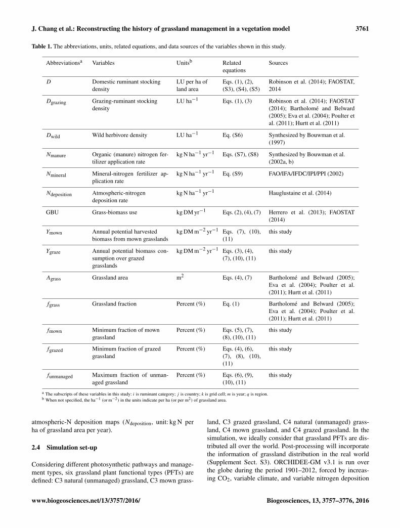
Table 1. The abbreviations, units, related equations, and data sources of the variables shown in this study.
Abbreviationsa Variables Unitsb Relatedequations
Sources
D Domestic ruminant stockingdensity
LU per ha ofland area
Eqs. (1), (2),(S3), (S4), (S5)
Robinson et al. (2014); FAOSTAT,2014
Dgrazing Grazing-ruminant stockingdensity
LU ha−1 Eqs. (1), (3) Robinson et al. (2014); FAOSTAT(2014); Bartholomé and Belward(2005); Eva et al. (2004); Poulter etal. (2011); Hurtt et al. (2011)
Dwild Wild herbivore density LU ha−1 Eq. (S6) Synthesized by Bouwman et al.(1997)
Nmanure Organic (manure) nitrogen fer-tilizer application rate
kg N ha−1 yr−1 Eqs. (S7), (S8) Synthesized by Bouwman et al.(2002a, b)
Nmineral Mineral-nitrogen fertilizer ap-plication rate
kg N ha−1 yr−1 Eq. (S9) FAO/IFA/IFDC/IPI/PPI (2002)
Ndeposition Atmospheric-nitrogendeposition rate
kg N ha−1 yr−1 Hauglustaine et al. (2014)
GBU Grass-biomass use kg DM yr−1 Eqs. (2), (4), (7) Herrero et al. (2013); FAOSTAT(2014)
Ymown Annual potential harvestedbiomass from mown grasslands
kg DM m−2 yr−1 Eqs. (7), (10),(11)
this study
Ygraze Annual potential biomass con-sumption over grazedgrasslands
kg DM m−2 yr−1 Eqs. (3), (4),(7), (10), (11)
this study
Agrass Grassland area m2 Eqs. (4), (7) Bartholomé and Belward (2005);Eva et al. (2004); Poulter et al.(2011); Hurtt et al. (2011)
fgrass Grassland fraction Percent (%) Eq. (1) Bartholomé and Belward (2005);Eva et al. (2004); Poulter et al.(2011); Hurtt et al. (2011)
fmown Minimum fraction of mowngrassland
Percent (%) Eqs. (5), (7),(8), (10), (11)
this study
fgrazed Minimum fraction of grazedgrassland
Percent (%) Eqs. (4), (6),(7), (8), (10),(11)
this study
funmanaged Maximum fraction of unman-aged grassland
Percent (%) Eqs. (6), (9),(10), (11)
this study
a The subscripts of these variables in this study: i is ruminant category; j is country; k is grid cell; m is year; q is region.b When not specified, the ha−1 (or m−2) in the units indicate per ha (or per m2) of grassland area.
atmospheric-N deposition maps (Ndeposition, unit: kg N perha of grassland area per year).
2.4 Simulation set-up
Considering different photosynthetic pathways and manage-ment types, six grassland plant functional types (PFTs) aredefined: C3 natural (unmanaged) grassland, C3 mown grass-
land, C3 grazed grassland, C4 natural (unmanaged) grass-land, C4 mown grassland, and C4 grazed grassland. In thesimulation, we ideally consider that grassland PFTs are dis-tributed all over the world. Post-processing will incorporatethe information of grassland distribution in the real world(Supplement Sect. S3). ORCHIDEE-GM v3.1 is run overthe globe during the period 1901–2012, forced by increas-ing CO2, variable climate, and variable nitrogen deposition
www.biogeosciences.net/13/3757/2016/ Biogeosciences, 13, 3757–3776, 2016
3762 J. Chang et al.: Reconstructing the history of grassland management in a vegetation model
fgrazed fmown funmanaged
Ygrazed Ymown
Agrass GBU
Dgrazing Dwild Nmanure Nmineral Ndeposition
ORCHIDEE-GM
Unmanaged grassland
Mown grassland
Grazed grassland
Input maps
Model simulation
Model Output
Data used as constraint
Management intensity maps
��
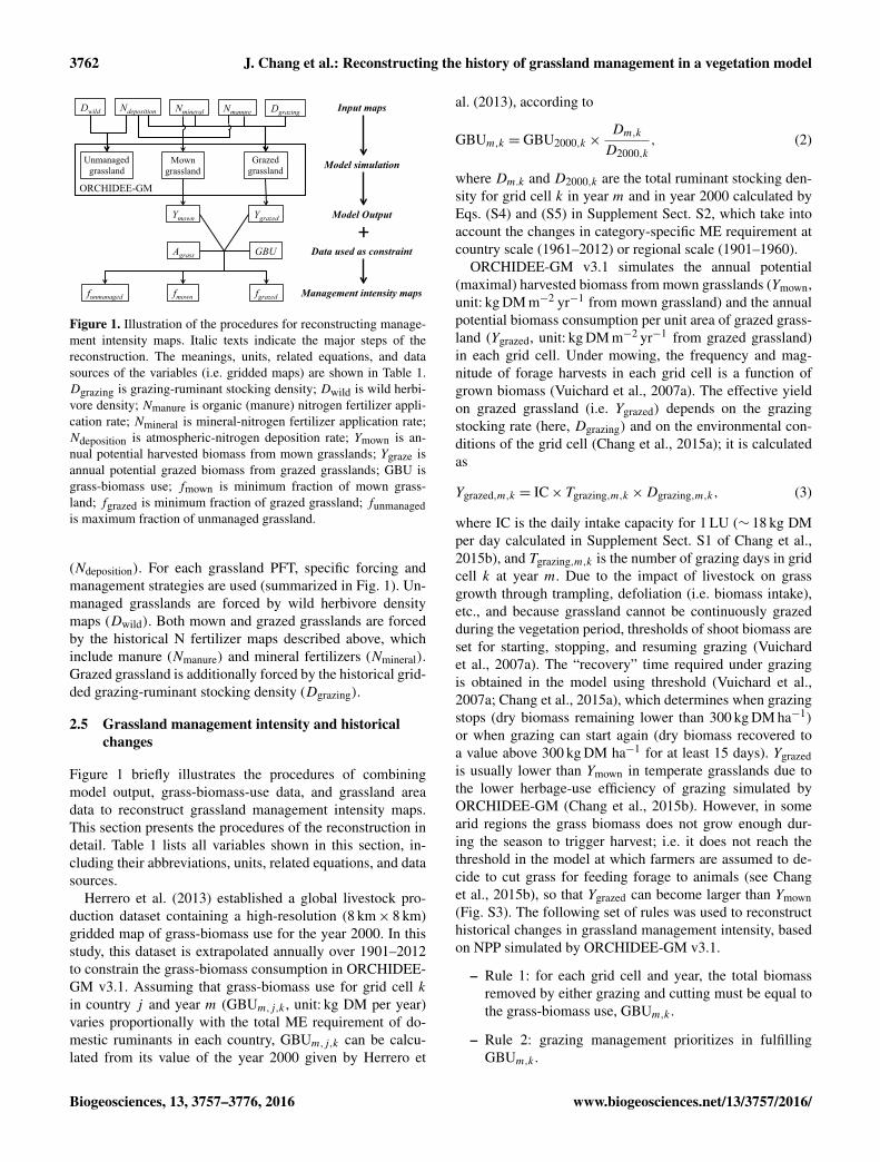
Figure 1. Illustration of the procedures for reconstructing manage-ment intensity maps. Italic texts indicate the major steps of thereconstruction. The meanings, units, related equations, and datasources of the variables (i.e. gridded maps) are shown in Table 1.Dgrazing is grazing-ruminant stocking density; Dwild is wild herbi-vore density; Nmanure is organic (manure) nitrogen fertilizer appli-cation rate; Nmineral is mineral-nitrogen fertilizer application rate;Ndeposition is atmospheric-nitrogen deposition rate; Ymown is an-nual potential harvested biomass from mown grasslands; Ygraze isannual potential grazed biomass from grazed grasslands; GBU isgrass-biomass use; fmown is minimum fraction of mown grass-land; fgrazed is minimum fraction of grazed grassland; funmanagedis maximum fraction of unmanaged grassland.
(Ndeposition). For each grassland PFT, specific forcing andmanagement strategies are used (summarized in Fig. 1). Un-managed grasslands are forced by wild herbivore densitymaps (Dwild). Both mown and grazed grasslands are forcedby the historical N fertilizer maps described above, whichinclude manure (Nmanure) and mineral fertilizers (Nmineral).Grazed grassland is additionally forced by the historical grid-ded grazing-ruminant stocking density (Dgrazing).
2.5 Grassland management intensity and historicalchanges
Figure 1 briefly illustrates the procedures of combiningmodel output, grass-biomass-use data, and grassland areadata to reconstruct grassland management intensity maps.This section presents the procedures of the reconstruction indetail. Table 1 lists all variables shown in this section, in-cluding their abbreviations, units, related equations, and datasources.
Herrero et al. (2013) established a global livestock pro-duction dataset containing a high-resolution (8 km× 8 km)gridded map of grass-biomass use for the year 2000. In thisstudy, this dataset is extrapolated annually over 1901–2012to constrain the grass-biomass consumption in ORCHIDEE-GM v3.1. Assuming that grass-biomass use for grid cell k
in country j and year m (GBUm,j,k , unit: kg DM per year)varies proportionally with the total ME requirement of do-mestic ruminants in each country, GBUm,j,k can be calcu-lated from its value of the year 2000 given by Herrero et
al. (2013), according to
GBUm,k = GBU2000,k ×Dm,k
D2000,k
, (2)
where Dm.k and D2000,k are the total ruminant stocking den-sity for grid cell k in year m and in year 2000 calculated byEqs. (S4) and (S5) in Supplement Sect. S2, which take intoaccount the changes in category-specific ME requirement atcountry scale (1961–2012) or regional scale (1901–1960).
ORCHIDEE-GM v3.1 simulates the annual potential(maximal) harvested biomass from mown grasslands (Ymown,unit: kg DM m−2 yr−1 from mown grassland) and the annualpotential biomass consumption per unit area of grazed grass-land (Ygrazed, unit: kg DM m−2 yr−1 from grazed grassland)in each grid cell. Under mowing, the frequency and mag-nitude of forage harvests in each grid cell is a function ofgrown biomass (Vuichard et al., 2007a). The effective yieldon grazed grassland (i.e. Ygrazed) depends on the grazingstocking rate (here, Dgrazing) and on the environmental con-ditions of the grid cell (Chang et al., 2015a); it is calculatedas
Ygrazed,m,k = IC× Tgrazing,m,k ×Dgrazing,m,k, (3)
where IC is the daily intake capacity for 1 LU (∼ 18 kg DMper day calculated in Supplement Sect. S1 of Chang et al.,2015b), and Tgrazing,m,k is the number of grazing days in gridcell k at year m. Due to the impact of livestock on grassgrowth through trampling, defoliation (i.e. biomass intake),etc., and because grassland cannot be continuously grazedduring the vegetation period, thresholds of shoot biomass areset for starting, stopping, and resuming grazing (Vuichardet al., 2007a). The “recovery” time required under grazingis obtained in the model using threshold (Vuichard et al.,2007a; Chang et al., 2015a), which determines when grazingstops (dry biomass remaining lower than 300 kg DM ha−1)
or when grazing can start again (dry biomass recovered toa value above 300 kg DM ha−1 for at least 15 days). Ygrazedis usually lower than Ymown in temperate grasslands due tothe lower herbage-use efficiency of grazing simulated byORCHIDEE-GM (Chang et al., 2015b). However, in somearid regions the grass biomass does not grow enough dur-ing the season to trigger harvest; i.e. it does not reach thethreshold in the model at which farmers are assumed to de-cide to cut grass for feeding forage to animals (see Changet al., 2015b), so that Ygrazed can become larger than Ymown(Fig. S3). The following set of rules was used to reconstructhistorical changes in grassland management intensity, basedon NPP simulated by ORCHIDEE-GM v3.1.
– Rule 1: for each grid cell and year, the total biomassremoved by either grazing and cutting must be equal tothe grass-biomass use, GBUm,k .
– Rule 2: grazing management prioritizes in fulfillingGBUm,k .
Biogeosciences, 13, 3757–3776, 2016 www.biogeosciences.net/13/3757/2016/

J. Chang et al.: Reconstructing the history of grassland management in a vegetation model 3763
– Rule 3: if the potential biomass consumption from graz-ing (Ygrazed) is not high enough to fulfil GBUm,j,k , acombination of grazing and mowing management istaken.
Thus, for grid cell k in year m, the minimum frac-tion of grazed (fgrazed,m,k), the minimum fraction of mown(fmown,m,k), and the maximum fraction of unmanaged grass-land (funmanaged,m,k) are calculated with the following equa-tions (definitions of minimum and maximum in this contextare given below).
If Agrass,m,k ×Ygrazed,m,k > GBUm,k , then
fgrazed,m,k =GBUm,k
Agrass,m,k ×Ygrazed,m,k
(4)
fmown,m,k = 0 (5)funmanaged,m,k = 1− fgrazed,m,k, (6)
where Agrass,m,k (unit: m2) is the grassland area for grid cellk in year m of the series of historic land-cover change maps(Supplement Sect. S3).
If Agrass,m,k ×Ygrazed,m,k < GBUm,k and Agrass,m,k ×
Ymown,m,k > GBUm,k then
fgrazed,m,k ×Agrass,m,k ×Ygrazed,m,k + fmown,m,k
×Agrass,m,k ×Ymown,m,k = GBUm,k (7)fgrazed,m,k + fmown,m,k = 1 (8)funmanaged,m,k = 0. (9)
If GBUm,k cannot be fulfilled by any combination of mod-elled Ygrazed and Ymown, we diagnose a modelled grass-biomass production deficit and apply the following equa-tions:
if Ygrazed>Ymown, then fgrazed,m,k = 1, fmown,m,k = 0,
and funmanaged,m,k = 0, (10)if Ygrazed<Ymown, then fmown,m,k = 1, fgrazed,m,k = 0,
and funmanaged,m,k = 0. (11)
This set of equations is valid for a mosaic of different typesof grasslands in each grid cell, some managed (grazed and/ormown) and some remaining unmanaged. In reality, (1) farmowners could increase the mown fraction to produce moreforage, which corresponds approximately to the mixed andlandless systems of Bouwman et al. (2005); and (2) animalscould migrate a long way across grazed and unmanaged frac-tions (as they do in real rangelands) and only select the mostdigestible grass in pastoral systems, which corresponds to ex-tensively grazed grasslands. Yet, given the approximationsmade in this study, fgrazed,m,k and fmown,m,k represent theminimum fractions of grazed/mown grasslands rather thanthe actual fractions, and funmanaged,m,k corresponds to a max-imum fraction of unmanaged grasslands since both mixedand landless and extensive grazing are not modelled.
Herbage-use efficiency (Hodgson, 1979) is defined as theforage removed expressed as a proportion of herbage growth.It can be an indicator of management intensity over managedgrassland, in addition to the fraction of managed area ob-tained above. In this study, the forage removed is modelledannual grass-biomass use including Ygrazed and Ymown, andherbage growth is modelled annual grass GPP.
2.6 Model evaluation: datasets and model–dataagreement metrics
The gridded grassland management intensity maps are modeldependent because they depend on modelled productiv-ity. Thus the evaluation of modelled productivity becomesnecessary. In this study, modelled productivity (NPP andGPP) is compared to a new set of site-level NPP measure-ments (Sect. 2.7.1) and two satellite-based models of GPP(MODIS-GPP, from the Moderate Resolution Imaging Spec-troradiometer, Sect. 2.7.2; sun-induced chlorophyll fluores-cence (SIF) data, Sect. 2.7.3). Modelled NPP (or GPP) com-bines grassland productivity of all PFTs (Sect. 2.4), account-ing for the variable fractions of grazed, mown, and un-managed grassland in each grid cell calculated by Eqs. (4–11), and hereafter is referred to as NPPmodel (or GPPmodel).Model–data agreement of NPP and GPP was assessed usingPearson’s product-moment correlation coefficients (r) androot mean squared errors (RMSEs).
2.6.1 Grassland NPP observation database
NPP is a crucial variable in vegetation models and it isessential that this variable is properly validated. High-qualitymeasurements of grassland NPP are scarce, partly due to thedifficulty of measuring some NPP components such as fine-root production (Scurlock et al., 1999, 2002). An updatedversion of the Luyssaert et al. (2007) database comprisingnon-forest biomes (Campioli et al., 2015) was used here. Thisdatabase contains a flag indicating managed or unmanagedto each site and provides mean annual temperature, annualprecipitation, and downwelling solar radiation based on sitemeasurements from the literature, CRU database (Mitchelland Jones, 2005), MARS database (http://mars.jrc.ec.europa.eu/mars/About-us/AGRI4CAST/Data-distribution/AGRI4CAST-Interpolated-Meteorological-Data), or World-Clim database (Hijmans et al., 2005). Three additionaldatasets used in this study present NPP measurements from30 sites across China (Zeng et al., 2015; Y. Bai, personalcommunication, 2015) and 16 sites across western Siberia(Peregon et al., 2008; with data updated to 2012). Data fromChina include NPP observations at fenced (i.e. unmanaged)and unfenced (i.e. managed) grassland for each site, and dataof western Siberia are observations from natural wetland.In total, we have 305 NPP observations (NPPobs) withseparated aboveground and belowground NPP from 129sites all over the world (including grassland, wetland, and
www.biogeosciences.net/13/3757/2016/ Biogeosciences, 13, 3757–3776, 2016
3764 J. Chang et al.: Reconstructing the history of grassland management in a vegetation model
savanna; Fig. S4). Duplicate observations from the samesite year were averaged and considered as a single entry.NPP measurements with different management (managed orunmanaged) at the same site were considered as identicalobservations. In total, 270 grassland NPP measurementswere compared to the simulation of ORCHIDEE-GM v3.1for the grid cell, corresponding to each site and for the timeperiod of observation. Depending on the status of measuredgrassland (unmanaged or managed), modelled NPP fromunmanaged or managed grassland is used for comparison.Modelled NPP over managed grassland accounts for the NPPfrom mown and grazed grassland and their correspondingfractions.
2.6.2 Grassland GPP from MODIS products
The MOD17A3 dataset (version 55; Zhao et al., 2005;Zhao and Running, 2010) – a MODIS product on vege-tation production – provides the seasonal and annual GPPdata at a spatial resolution of 1 km from 2000 to 2013.To obtain the grassland GPP from the MOD17 dataset,we first extract the MOD17 GPP at 1 km resolution overgrassland grids in the MOD12Q1 dataset. Here, the grass-land in the MOD12Q1 dataset includes the “open shrub-land”, “savanna”, and “grassland” in the Boston University’sUMD classification scheme. The extracted annual and sea-sonal MODIS GPP was then averaged and aggregated to0.5◦× 0.5◦ spatial resolution to be comparable to model out-put.
2.6.3 Sun-induced chlorophyll fluorescence data
Space-based observations of SIF provide a time-resolvedmeasurement of a proxy of photosynthesis (Guanter et al.,2014). Similar to the MPI-BGC data-driven GPP product(Jung et al., 2011), SIF values exhibit a linear relationship(r2= 0.79) with monthly tower GPP at grassland sites in
western Europe (Guanter et al., 2014). Compared to MODISEVI (MOD13C2 products), SIF observations drop to zeroduring the non-growing season, thus providing a clearer sig-nal of photosynthetic activity (Guanter et al., 2014) thanother vegetation indices based on visible and near-infraredreflectances. SIF also provides a better seasonal agreementwith GPP from flux towers as compared to vegetation indices(Joiner et al., 2014).
In this study, we used monthly GOME-2 (version 26, level3) SIF data products with the spatial resolution of 0.5◦× 0.5◦
(available from 2007 to 2012). SIF-GPP is calculated by aSIF-GPP linear model adjusted from Guanter et al. (2014)(SIF-GPP = −0.1 + 4.65 × SIF (V26); see SupplementSect. S6 for detail). To reduce the contamination of SIF bynon-grassland PFTs, we restrict the model–data compari-son to grassland-dominated grid cells, defined as those withgrassland cover in the MOD12Q1 dataset (Sect. 2.5.2) islarger than 50 %.
3 Results
3.1 Maps of grassland management intensity
Figure 2 shows the minimum fractions of mown and grazedgrasslands and the maximum fraction of unmanaged out oftotal grassland (fmown, fgrazed, and funmanaged respectively;Sect. 2.4) in the year 2000. Grazed grasslands comprise mostof the managed grasslands in the maps (Fig. 2b). Signif-icant fractions of mown grasslands are only found in re-gions with high ruminant stocking density such as east-ern China, India, eastern and northern Europe, and easternUnited States, where Ygrazed cannot fulfil the grass-biomassdemand (Fig. 2a). Using the FAO-defined regions (see cap-tion to Table 2), the largest fractions of managed grasslandsare modelled in regions of high ruminant stocking density(Fig. S1) such as in eastern Europe with a mean fractionof 90± 17 % (the mean is the average fraction of mownand grazed grasslands over all the grid cells in this region,and the standard deviation is taken from differences be-tween grid cells), South Asia (59± 46 %), and western Eu-rope (55± 36 %). The lowest managed grasslands fractionsare modelled in the Russian Federation (17± 34 %).
In some grid cells, the simulated grassland productivity isnot sufficient to fulfil the grass-biomass use given by Her-rero et al. (2013; Fig. 2d). Of the 2.4 billion tonnes of grass-biomass use (in dry matter for the reference year 2000) givenby Herrero et al., 16 % cannot be fulfilled by the produc-tivity simulated by ORCHIDEE-GM v3.1. This translatesinto a modelled grass-biomass production deficit of 0.38 bil-lion tonnes (Table 2). Out of all regions, the largest mod-elled production deficit (fglobal in Table 2) is found in SouthAsia (49 %). This South Asian deficit is predominantly in In-dia (35 % of the modelled global total deficit) and Pakistan(10 % of the modelled global total deficit). Other regions witha biomass production deficit are the Near East and NorthAfrica (18 %) and sub-Saharan Africa (13 %). Overall, 32 %of the global production deficit comes from regions with dryclimate and low NPP (less than 50 g C m−2yr−1), and 34 %of it comes from regions with low grassland cover (less than10 % of total land cover). The causes of this grass-biomassproduction deficit diagnosed by ORCHIDEE-GM are dis-cussed in Sect. 4.2.
Modelled herbage-use efficiency over managed grasslandduring the 2000s (grazed plus mown; Fig. 3) ranges between2 and 20 % in most regions and generally follows the spatialpattern of grazing-ruminant density (Fig. S1). High herbage-use efficiency (over 20 %) is found in regions with signif-icant mown grassland (fmown) simulated due to the largerfraction of biomass removed over mown grassland than thatover grazed grassland in the same grid cell (Fig. S3).
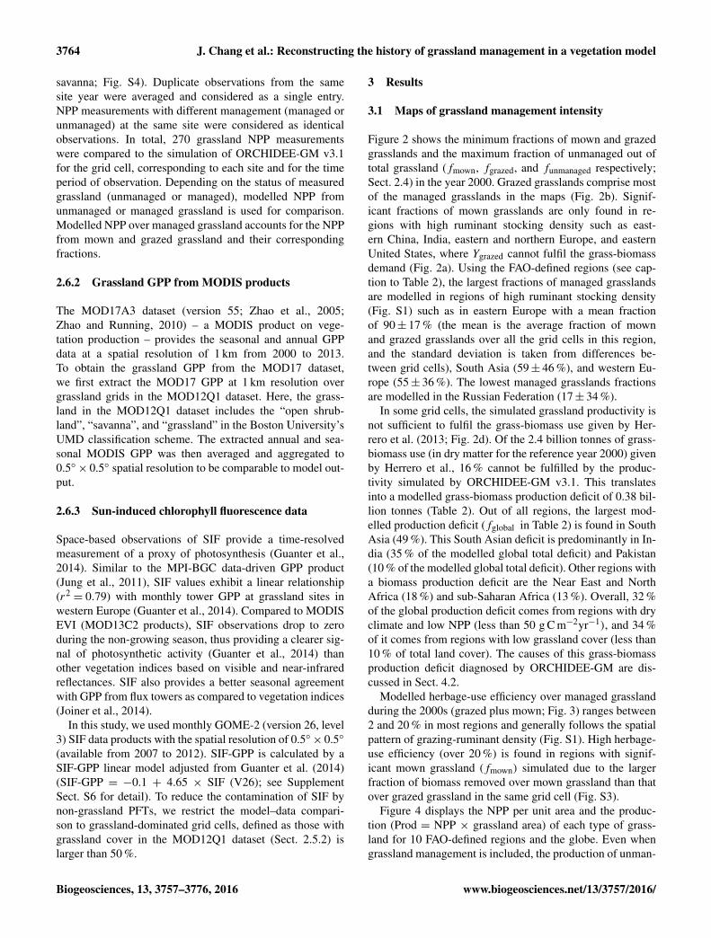
Figure 4 displays the NPP per unit area and the produc-tion (Prod = NPP × grassland area) of each type of grass-land for 10 FAO-defined regions and the globe. Even whengrassland management is included, the production of unman-
Biogeosciences, 13, 3757–3776, 2016 www.biogeosciences.net/13/3757/2016/

J. Chang et al.: Reconstructing the history of grassland management in a vegetation model 3765
Figure 2. (a) Mown, (b) grazed, and (c) unmanaged fraction of global grassland, and (d) modelled grass-biomass production deficit of2000. Modelled grass-biomass production deficit indicates the simulated grassland productivity in the grid cells is not sufficient to fulfil thegrass-biomass use given by Herrero et al. (2013) and is expressed with units of g dry matter (DM) per m2 of total land area in each grid cell.
Table 2. Grass-biomass production deficits in regions where simulated productivity by ORCHIDEE-GM v3.1 (i.e. Ymown and Ygrazed; seetext) cannot fulfil the grass-biomass use given by Herrero et al. (2013) for 2000.
Regionsa Grass-biomass use Production deficit fdeficit fglobal(million tonne DM) (million tonne DM) (%)b (%)c
North America 228 19 8 % 5 %Russian Federation 52 1 2 % 0.3 %Western Europe 196 5 2 % 1 %Eastern Europe 82 1 1 % 0.3 %Near East and North Africa 175 67 39 % 18 %East and Southeast Asia 275 25 9 % 7 %Oceania 107 4 3 % 1 %South Asia 390 188 48 % 49 %Latin America and Caribbean 534 23 4 % 6 %Sub-Saharan Africa 351 48 14 % 13 %World total 2391 380 16 % 100 %
a Regions are classified following the definition in the FAO Global Livestock Environmental Assessment Model (GLEAM;http://www.fao.org/gleam/en/).b fdeficit is the fraction of production deficit in the total grass-biomass use of the region for 2000.c fglobal is the fraction of production deficit in the global total production deficit for 2000.
aged grassland (Produnmanaged) still comprises 63 % of thetotal production (Prodtotal) in the 1990s. The production ofgrazed grasslands (Prodgrazed) accounts for 34 % of Prodtotal,while the production of mown grasslands (Prodmown) is only3 %, given the small area under this management practice(Fig. 4). Mown grasslands only contribute to production inthe regions where climate conditions and fertilizers maintaina high NPP, and Ygrazedis not enough to fulfil the animal re-quirement, which triggers the harvest practice in Eqs. (7–11).
Over unmanaged grassland (Fig. S2), ORCHIDEE-GMv3.1 simulated a total annual consumption by wild herbivoresof 147–654 million tonnes DM of the 5778 million tonnes
DM in aboveground NPP (consumable NPP) over suitablegrassland (Table S5), which comprises 3–11 % of the con-sumable NPP, similar to the range given by Warneck (1988).The fraction of consumption in consumable NPP varied from1 % in the former USSR to 9 % in Scandinavia, indicating thedifferent significance of wild herbivores on grassland.
3.2 Historical changes in the area and productivity ofmanaged grassland
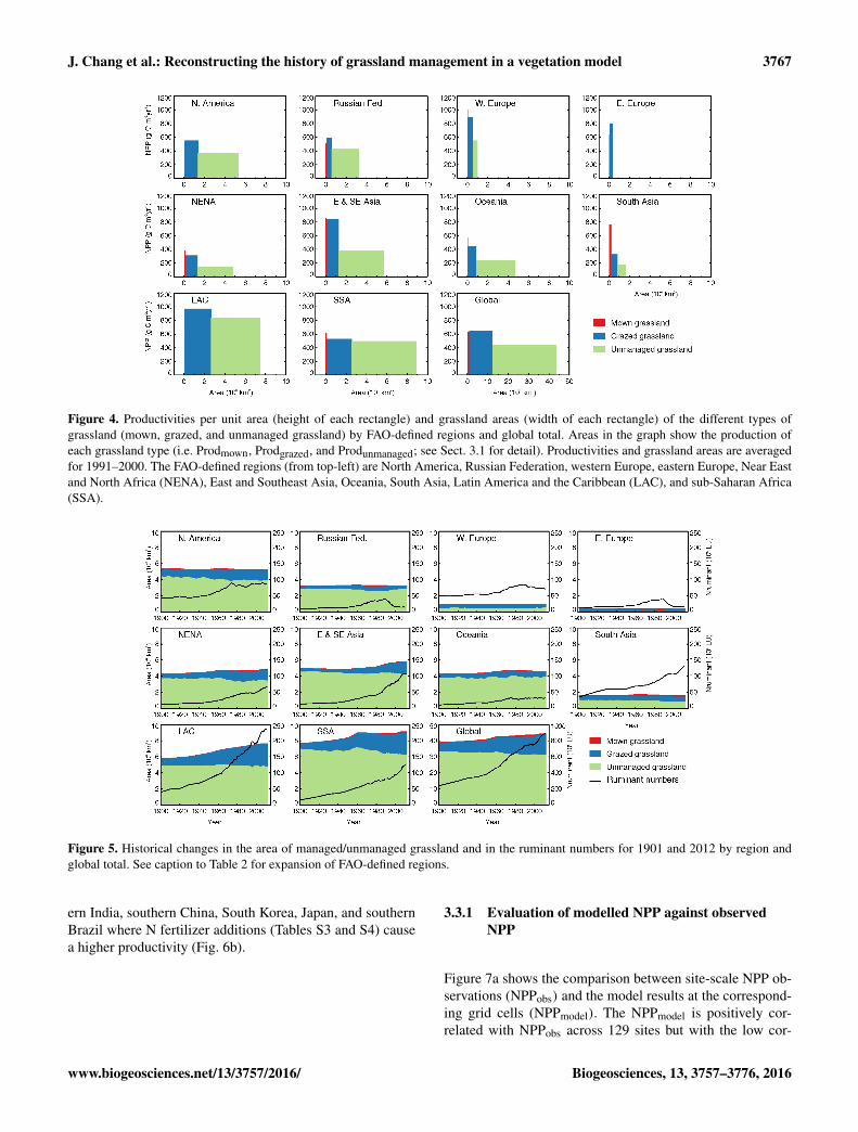
The global minimum area of managed grassland(Amanaged-gm) is of 6.1× 10⁶ km2 in 1901 and increased to12.3× 106 km2 in 2000 (Table 3; Fig. 5) – an increase of
www.biogeosciences.net/13/3757/2016/ Biogeosciences, 13, 3757–3776, 2016

3766 J. Chang et al.: Reconstructing the history of grassland management in a vegetation model
Table 3. Area, mean productivity, and herbage-use efficiency of managed grassland from this study, ruminant numbers, and pasture areafrom HYDE 3.1 dataset for 1901 and 2000 by regions and global total.
Regionsa Grassland area Mean productivity Herbage-use Nruminantc Pasture area from
(1000 km2; 1901/2000) (kg DM m2 yr−1; 1900s/1990sb) efficiency (Percent; (106 LU; HYDE 3.1d
Total managed Mown Grazed Ymown Ygrazed 1900s/1990s) 1901/2000) (1000 km2; 1901/2000)
North America 989/1360 41/95 948/1265 0.26/0.38 0.09/0.13 6.2 %/7.4 % 42/87 1157/2482Russian Federation 351/567 23/49 329/518 0.19/0.42 0.06/0.10 5.0 %/5.8 % 9/16 2995/904Western Europe 514/555 54/44 460/522 0.51/0.85 0.22/0.31 10.0 %/10.6 % 49/76 793/595Eastern Europe 339/366 71/93 268/274 0.26/0.54 0.11/0.21 7.1 %/9.8 % 12/17 655/248Near East and North Africa 595/1334 17/130 578/1205 0.09/0.18 0.05/0.06 6.3 %/6.2 % 12/50 2607/5607East and Southeast Asia 419/1271 6/77 412/1194 0.43/0.72 0.09/0.14 4.2 %/5.8 % 14/83 2998/5327Oceania 499/828 52/60 447/769 0.18/0.33 0.07/0.11 7.2 %/7.0 % 11/33 979/4000South Asia 614/830 123/202 491/628 0.32/0.58 0.10/0.12 10.4 %/14.0 % 35/109 651/962Latin America and Caribbean 960/2640 11/33 949/2608 0.35/0.39 0.11/0.18 4.1 %/5.2 % 40/194 1341/5446Sub-Saharan Africa 803/2561 8/109 795/2452 0.32/0.46 0.08/0.10 4.8 %/5.5 % 16/93 4486/6991Global total 6083/12 313 404/891 5679/11 422 0.29/0.48 0.10/0.14 6.2 %/6.6 % 238/759 19 181/32 764
a Regions are classified following the definition in the FAO Global Livestock Environmental Assessment Model (GLEAM; http://www.fao.org/gleam/en/).b The potential harvested biomass from mown grassland (Ycut) and the potential biomass consumption over grazed grassland (Ygraze) are 10-year averages for the period 1901–1910 (1900s) and 1991–2000 (1990s), representing theproductivity at the beginning and at the end of the 20th century respectively.c Ruminant numbers (in units of livestock unit, LU) are calculated based on the total metabolisable energy (ME) requirement by all ruminant. The ME requirement by all ruminants is based on ruminant numbers from statistics (for1961–2012; data derived from FAOSTAT, 2014) and literature estimates (for 1901–1960; data derived from Mitchell (1993, 1998a, b) and available in HYDE database athttp://themasites.pbl.nl/tridion/en/themasites/hyde/landusedata/livestock/index-2.html), using the calculation method given in the Supplement Sect. S1 of Chang et al. (2015a).d See Klein Goldewijk et al. (2011) for details.
Figure 3. Average herbage-use efficiency over managed grassland(grazed plus mown) in 2000–2009 simulated by ORCHIDEE-GMv3.1. Herbage-use efficiency (Hodgson, 1979) is defined as the for-age removed expressed as a proportion of herbage growth. In thisstudy, the forage removed is modelled annual grass-biomass use in-cluding Ygrazed and Ymown, and herbage growth is modelled annualgrass GPP.
102 % during the 20th century. This expansion of managedgrasslands is mainly explained by the increase in the areaof grazed lands (+5.7× 10⁶ km2), while mown grasslandincreased only marginally (+0.5× 10⁶ km2). The largestextension of Amanaged-gm is found in sub-Saharan Africa(+1.8× 10⁶ km2) and Latin America and the Caribbean(+1.7× 10⁶ km2; Fig. 5). The regions with the largestrelative expansion of managed grasslands (as a percentageof 1901 areas) are sub-Saharan Africa (+219 %), Eastand Southeast Asia (+204 %), nd Latin America and theCaribbean (+175 %), and the regions where the numberof domestic ruminants (Nruminant) increased by nearly orover a factor of 3. Only small increases of Amanaged-gmwere modelled in western Europe (+41× 103 km2; i.e. 8 %)and eastern Europe (+27× 103 km2; i.e. 8 %), despite anincrease of Nruminant by a factor of 1.5 in western Europe
(+27×106 LU) and of 1.4 in eastern Europe (+5× 10⁶ LU).This means that livestock production intensified in thosetwo regions, first by giving crop feedstock given to animals(Bouwman et al., 2005) and second through the optimizationof forage harvesting and grazing to feed higher animal-stocking densities. Note that the animal density in easternand western Europe peaked at 123× 106 LU near 1990 andhas declined by 29 % since then.
Besides the extension of managed grassland area, mod-elled herbage-use efficiency over managed grassland in-creased from 6.2 to 6.6 % during the 20th century, indicat-ing the intensification of grassland management. Large in-crease in herbage-use efficiency is modelled in South Asia(+3.6 %) and eastern Europe (+2.7 %), while marginal de-crease of herbage-use efficiency is found in the Near Eastand North Africa (−0.1 %) and Oceania (−0.2 %; Table 3).
The global mean potential productivity of mown grass-land (Ymown) increased by 62 % from 0.29 kg DM m−2 yr−1
for 1900s to 0.48 kg DM m−2 yr−1 for the 1990s, whilethat of grazed grassland Ygrazed increased by 40 %, from0.10 kg DM m−2 yr−1 for the 1900s to 0.14 kg DM m−2 yr−1
for the 1990s (Table 3). During the last century, Ymown in-creased by more than 40 % in most regions except in LatinAmerica and the Caribbean (14 %), while the increase ofYgrazed ranged from 25 % in sub-Saharan Africa and 80 % ineastern Europe (Table 3).
3.3 Evaluation of modelled productivity
Figure 6 shows the grassland productivity (NPPmodel;Fig. 6a) and the NPP differences between NPPmodel and NPPfrom unmanaged grassland (Fig. 6b). The effect of includingmanagement does not produce a big difference in simulatedNPP, which has similar patterns in most regions (Fig. 6b).Nevertheless, there are significant differences of NPP due tomanagement in the central United States, Europe, northeast-
Biogeosciences, 13, 3757–3776, 2016 www.biogeosciences.net/13/3757/2016/
J. Chang et al.: Reconstructing the history of grassland management in a vegetation model 3767
Figure 4. Productivities per unit area (height of each rectangle) and grassland areas (width of each rectangle) of the different types ofgrassland (mown, grazed, and unmanaged grassland) by FAO-defined regions and global total. Areas in the graph show the production ofeach grassland type (i.e. Prodmown, Prodgrazed, and Produnmanaged; see Sect. 3.1 for detail). Productivities and grassland areas are averagedfor 1991–2000. The FAO-defined regions (from top-left) are North America, Russian Federation, western Europe, eastern Europe, Near Eastand North Africa (NENA), East and Southeast Asia, Oceania, South Asia, Latin America and the Caribbean (LAC), and sub-Saharan Africa(SSA).
Figure 5. Historical changes in the area of managed/unmanaged grassland and in the ruminant numbers for 1901 and 2012 by region andglobal total. See caption to Table 2 for expansion of FAO-defined regions.
ern India, southern China, South Korea, Japan, and southernBrazil where N fertilizer additions (Tables S3 and S4) causea higher productivity (Fig. 6b).
3.3.1 Evaluation of modelled NPP against observedNPP
Figure 7a shows the comparison between site-scale NPP ob-servations (NPPobs) and the model results at the correspond-ing grid cells (NPPmodel). The NPPmodel is positively cor-related with NPPobs across 129 sites but with the low cor-
www.biogeosciences.net/13/3757/2016/ Biogeosciences, 13, 3757–3776, 2016

3768 J. Chang et al.: Reconstructing the history of grassland management in a vegetation model
Figure 6. Modelled mean grassland NPP (NPPmodel) for the period1990–1999 (a), and the NPP differences (b) between NPPmodel andNPP from unmanaged grassland only. NPPmodel combines grass-land productivity of all PFTs (Sect. 2.5), accounting for the variablefractions of grazed, mown, and unmanaged grassland in each gridcell calculated by Eqs. (4)–(11).
relation coefficient of r = 0.35 (p<0.01) and the RMSEof 380 g C m−2yr−1. Figure 7b presents box-and-whiskerplot of the observed and modelled annual whole-plant NPP,aboveground NPP, and belowground NPP. The mean valueand range of modelled whole-plant NPP are both higher thanthose of NPPobs. The NPP overestimation by the model ismainly due to a too-high aboveground NPP, while below-ground NPP is only little higher for its mean or even lowerfor its median than belowground NPPobs.
3.3.2 Evaluation of modelled GPP againstMODIS-GPP for annual mean and interannualvariability
At global scale, MODIS-GPP gives a mean grassland GPPof 537 g C m−2 yr−1 and ORCHIDEE-GM v3.1 simulatesa mean value of 796 g C m−2 yr−1, ≈ 50 % higher thanMODIS-GPP. A higher modelled GPP (GPPmodel) thanMODIS is found for all latitude bands especially in bo-real (50–80◦ N) and tropical regions (20◦ S–20◦ N; Fig. 8).The linear regression between gridded MODIS-GPP andGPPmodel suggests a similar spatial pattern (slope = 1.05,and the correlation coefficient rspatial = 0.84; Fig. S5).
The temporal correlation coefficient between the de-trended time series of global GPPmodel and MODIS-GPP wasfound to be high (rIAV-global 0.88, p<0.01). Within the grid
Figure 7. (a) Comparison between site observations of whole-plant NPP (NPPobs) and modelled NPP (NPPmodel); (b) box-and-whisker plot of the observed and modelled annual whole-plant NPP,aboveground NPP, and belowground NPP. In subplot (a), grass-land sites in different Köppen climate zones are specified by dif-ferent colours. The Köppen climate zones are classified based onPeel et al. (2007) using climate data from WorldClim (http://www.worldclim.org/). In subplot (b), the “whisker” indicates the cross-measurement (total 270 measurements) uncertainty.
cells covered by grass over more than 20 % of total land inMOD12Q1, significant positive interannual correlations be-tween GPPmodeland MODIS-GPP were found for 39 % of thegrid cells (i.e. 40 % of the grassland area), except in sometundra areas of Siberia and North America, grassland on theQinghai–Tibet Plateau, and savannah in sub-Saharan Africa(Fig. 9).
3.3.3 Evaluation of modelled seasonal cycle of GPPagainst MODIS-GPP and GOME-2 SIF products
Figure 10 compares the normalized seasonal variation ofGPPmodel, MODIS-GPP, and SIF-GPP for five latitude bandsand the globe. Similar mean seasonal variations of grasslandproductivity are found between modelled GPP, MODIS-GPP,and SIF (rseasonal range from 0.55 to 0.89; Table 4). Com-pared to both MODIS-GPP and SIF data, ORCHIDEE-GMv3.1 captures the seasonal variation of productivity in bo-
Biogeosciences, 13, 3757–3776, 2016 www.biogeosciences.net/13/3757/2016/

J. Chang et al.: Reconstructing the history of grassland management in a vegetation model 3769
Table 4. Mean ± standard deviation of rseasonal comparing the seasonal cycle of modelled GPP (GPPmodel), MODIS-GPP, and SIF data forthe five latitude bands and global scale. rseasonal is expressed as mean ± standard deviation of grid level correlation coefficient within eachlatitude band and global. To avoid the strong impact of other land-cover types (e.g. crop and forest) to the seasonal cycle, we only considerrseasonal for grid cells with grassland covering more than 50 % of total land in the MOD12Q1 dataset.
rseasonal Latitude bands Global
60–90◦ N 30–60◦ N 0–30◦ N 0–30◦ S 30–60◦ S
GPPmodel vs. SIF data 0.84± 0.15 0.81± 0.19 0.66± 0.27 0.68± 0.28 0.55± 0.33 0.77± 0.23GPPmodel vs. MODIS-GPP 0.89± 0.10 0.86± 0.16 0.71± 0.30 0.63± 0.44 0.63± 0.31 0.80± 0.27MODIS-GPP vs. SIF data 0.90± 0.11 0.87± 0.16 0.80± 0.22 0.61± 0.37 0.61± 0.36 0.81± 0.25
Figure 8. Comparison between mean MODIS-GPP and modelledGPP for the period 2000–2013 by latitude band. The uncertainty ofMODIS-GPP comes from the reported relative error term driven byNASA’s Data Assimilation Office (DAO) reanalysis datasets (Zhaoet al., 2006). The uncertainty of modelled GPP is the standard devi-ation of interannual variation of grassland GPP in each band for theperiod 2000–2013.
Figure 9. Spatial distribution of rIAV between MODIS-GPP andGPPmodel. rIAV is the correlation coefficient between detrendedtime series of modelled and MODIS-GPP from 2000 to 2012. Thisfigure only shows the rIAV for grid cells with grassland coveringmore than 20 % of total land in the MOD12Q1 dataset. Grey indi-cates insignificant or negative rIAV (p>0.05 or rIAV<0); yellow-to-red indicates significant positive rIAV with increasing value(rIAV>0 and p<0.05).
real and temperate regions of the Northern Hemisphere well(rseasonal >0.8; Table 4). In the band from 60◦ S to 30◦ N, rel-atively low average rseasonal correlations are found both withMODIS-GPP and SIF (ranging from 0.55 to 0.71). However,note that the rseasonal between the two remote sensing GPP re-lated products is relatively low for grassland between 60◦ Sand 30◦ N, particularly between 0 and 60◦ S (Table 4).
4 Discussion
4.1 Managed area of grassland and managementintensity: comparison with previous estimates
The area of managed grasslands obtained in this study islower than the pasture area of HYDE 3.1 (Apasture-hyde, KleinGoldewijk et al., 2011; Table 3), except in eastern Europefor the year 2000. Apasture-hyde is 3.2 times larger than theminimum area of managed grasslands (mown plus grazedgrasslands; hereafter referred to as Amanaged-gm) in the year1901 and 2.7 times larger in the year 2000. The differencecomes from the method used for estimating managed ar-eas between Klein Goldewijk et al. (2011) and this study.Apasture-hyde in Klein Goldewijk et al. (2011) was estimatedsimply from population density and the country-level-per-capita use of pasture derived from the FAO statistics (FAO-STAT, 2008). In this study, Amanaged-gm is constrained bygrass-biomass-use data (i.e. requirement of biomass for an-imals) and the simulated grassland productivity (i.e. supplyof biomass to animals). In fact, the actual (real-world) man-aged grassland area could be larger than Amanaged-gm in re-gions where grasslands are not strictly unmanaged, i.e. notfully occupied by Amanaged-gm in the management intensitymaps (i.e. funmanaged>0; Fig. 2c). In pastoral systems such asopen rangeland and mountain areas, animals keep moving tosearch for the most digestible grass. Tracts of grasslands canbe grazed for a short period, with only a small part of the an-nual grass productivity being digested (i.e. very low herbage-use efficiency). This type of grassland could be recognizedas extensively grazed grassland, whereas it is considered asunmanaged in this study. For example, lower herbage-useefficiency than that simulated in this study (Fig. 3) couldbe expected in open rangeland of central Asia, the Rus-
www.biogeosciences.net/13/3757/2016/ Biogeosciences, 13, 3757–3776, 2016

3770 J. Chang et al.: Reconstructing the history of grassland management in a vegetation model
Figure 10. The normalized seasonal variation of modelled GPP (GPPmodel), MODIS-GPP, and SIF for five latitude bands (a–e) and (f)global average.
sia federation, sub-Saharan Africa, Brazil, and Australia andin the mountains of southwestern China and the EuropeanAlps. Reclassifying these areas would result in a larger areaof extensively managed grassland. Few studies reported theherbage-use efficiency of managed grassland. One exceptionis the network of European eddy-covariance flux sites. Forthese sites the average herbage-use efficiency (expressed asforage defoliated as a proportion of GPP) is 7.1%± 6.1%for grazed sites, and 13.3%± 6.4 % for mown sites (J.-F.Soussana, personal communication, 2015); a similar range,between 2 and 20 %, is simulated in this study (Fig. 3).
The time evolution of Amanaged-gm since 1901 in this studyis arguably more realistic than HYDE because it considerschanges in animal stocking density from statistics and theevolution in per-head use of pasture. Amanaged-gm takes intoaccount (1) changes in grass-biomass requirement, consider-ing both ruminant numbers and meat/milk productivity (Sup-plement Sect. S2; Nruminant in Table 3); (2) changes in grass-land productivity driven by climate change, rising CO2 con-centration, and changes in N fertilization (Ymown and Ygrazedin Table 3); and (3) changes in management types (mownand grazed grassland areas in Table 3 and Fig. 5). For exam-ple in intensively managed grasslands, an increase in rumi-nant stocking density causes a shift from grazed to mowngrassland (globally and regionally, except in western Eu-rope; Table 3 and Fig. 5), because mown grassland providesmore grass biomass than grazed grassland per unit of area(Fig. S3).
Apasture-hyde is consistent with country-specific pasturearea censuses and thus may be suitable for reconstructingland cover, but it does not provide information about man-agement intensity. Amanaged-gm and its split between mown,grazed, and unmanaged fractions provide specific global dis-tributions of pasture management intensity and its historicalchanges. However, there are several limitations, which may
cause uncertainties in our maps of management intensity: (1)the grass fraction in ruminant diet has likely been changingduring the last century while, due to a lack of information,we assumed that it was static in each region up to the year2000; (2) technical developments (such as ruminant breed-ing) are not considered but may affect the feeding efficiency(meat/milk production per amount of feed) and thus feedbackon the grass-biomass requirement; (3) the spatial distributionof ruminants was kept constant in our estimate, whereas itcould have changed, depending on geographic changes inhuman population distribution; and (4) the results depend onthe accuracy of NPP modelling in ORCHIDEE-GM. Despitethese limitations, the maps of grassland management inten-sity provide new information for drawing up global estimatesof management impact on biomass production and yields(Campioli et al., 2015) and for global vegetation models likeORCHIDEE-GM to enable simulations of carbon stocks andGHG budgets beyond simple tuning of grassland productiv-ities (e.g. like in LPJmL; Bondeau et al., 2007) to accountfor management. These maps can also be tested in other veg-etation models, or the same algorithm can be implementedin other models to give the management intensity consistentwith simulated NPP.
4.2 Causes of regional grass-biomass productiondeficits
Grass-biomass production is constrained by the griddedbiomass consumption for the year 2000 (Herrero et al.,2013). In some grid cells, the gridded biomass consumptionby year 2000 cannot be fulfilled by the potential grass pro-duction simulated by ORCHIDEE-GM v3.1 (Fig. 2d). Thesemodelled grass-biomass production deficits could be due toseveral reasons.
Biogeosciences, 13, 3757–3776, 2016 www.biogeosciences.net/13/3757/2016/
J. Chang et al.: Reconstructing the history of grassland management in a vegetation model 3771
– Land-cover maps used as input to ORCHIDEE-GMv3.1 do not represent grasslands well in the mixed andlandless systems and grasslands providing occasionalfeed to ruminant (e.g. roadside, forest understory graz-ing land, and small patches). This failing could causethe model to miss a significant part of grass produc-tivity in this study. For example, the largest modelledgrass-biomass production deficit is found in India be-cause the simulated grassland productivity is far fromagreeing with the grass-biomass-use data. In this coun-try, occasional feed may constitute an important frac-tion of ruminant diet (30 or 50 % in mixed and landlessor pastoral systems of South Asia from Bouwman et al.,2005), which is not represented by the land-cover mapsused as input to ORCHIDEE-GM v3.1 and thus is notmodelled.
– In arid regions such as Pakistan, Sudan, Iran, Egypt,and northwestern China, grass can grow in places wherethe water table is near to the surface and groundwa-ter resources are available (e.g. oases, riparian zones,lakes). However, ORCHIDEE-GM v3.1 is driven bygridded climate data and does not taken into accountlocal topography-dependent water resources such asrivers and lakes and thus is not being able to simulatelocal grass growing areas in arid regions.
– Grassland irrigation, though it is not as common as incropland, is applied in arid regions such as Saudi Arabiabut is not considered by ORCHIDEE-GM v3.1.
– In some semi-arid open rangeland, ruminants may walklong distances to acquire enough grass. For example,in semi-arid sub-Saharan Africa, Uzbekistan, and cen-tral Australia, animals usually keep moving in order tosearch for grass. This displacement of grazing animalsfrom grass sources is not considered in the model.
– The grass fraction in ruminant diet is defined per re-gion according to specific production systems. How-ever, the grass fraction can differ within a region de-pending on local fodder crop production and grass-land use. For example, the large numbers of ruminantsin eastern China are mostly fed by grain and stovers(fibrous crop residues) instead of grass, because littlegrassland exists in that region.
4.3 Model performance: comparison of modelled andobserved grassland productivity
In Sect. 3.3, the spatial patterns of NPPmodel or GPPmodelwere compared with observations (NPPobs or MODIS-GPP). ORCHIDEE-GM v3.1 captured well the spatial pat-tern of grassland productivity, with (i) high rspatial betweenGPPmodel and MODIS-GPP (Sect. 3.3.2) and (ii) NPPmodelextracted from global simulation showing significant corre-lation with site-level NPP observation from 129 sites all over
the world (Sect. 3.3.1). However, GPPmodel is higher thanMODIS-GPP in all latitude bands (Fig. 8). It should be keptin mind that MODIS-GPP had a calculated 18 % uncertaintydue to climate forcing (Zhao et al., 2006). Besides, a lowbias of MODIS-GPP for grasslands has been reported in atallgrass prairie in the United States (Turner et al., 2006) andin an alpine meadow on the Tibetan Plateau (Zhang et al.,2008) when compared to the GPP from flux-tower measure-ments. The underestimate of MODIS-GPP is mostly relatedto the low value of the maximum light-use efficiency param-eters used in the MODIS-GPP algorithm (Turner et al., 2006;Zhang et al., 2008).
The relatively low r value between NPPmodel and site-levelNPPobs (r = 0.35, p<0.01; Sect. 3.3.1) could be related tothe fact that local climate, soil properties, and topographicfeatures are not considered in the model. For example, the r
between the site-level climate and that from the CRU+NCEPclimate forcing data (0.5◦× 0.5◦ resolution) is 0.96 for an-nual mean temperature but only 0.86 for annual total precip-itation and 0.86 for solar radiation. The relatively low corre-lation for annual total precipitation may cause inaccuracy inthe model simulations of productivity, because water avail-ability could be a major factor limiting grass growth (e.g. intemperate regions; Le Houerou et al., 1988; Silvertown et al.,1994; Briggs and Knapp 1995; Knapp et al., 2001; Nippert etal., 2006; Harpole et al., 2007). Further, a similar mean be-lowground NPP and an overestimation of mean abovegroundNPP by ORCHIDEE-GM v3.1 is found in Sect. 3.3.1, whichsuggests that (1) the model tends to overestimate above-ground NPP possibly due to overestimation of GPP (com-pared to MODIS-GPP) and (2) the model tends to overes-timate the ratio of aboveground and belowground biomassallocation (Rabove/below) compared to observation. This over-estimation could be the result of nitrogen limitation on thecarbon allocation scheme for grassland. For example, a largenitrogen supply has been observed to increase Rabove/below(Aerts et al., 1991; Cotrufo and Gorissen, 1997), while nitro-gen limitation might cause it to decrease. However, nitrogenlimitation in grassland is not accounted for in ORCHIDEE-GM v3.1, which possibly leads to the model’s overestimationof Rabove/below. The model could be improved by incorporat-ing the full nitrogen cycle.
For the seasonal cycle, we compared modelled GPPseasonality to both MODIS-GPP and GOME-2 SIF data.ORCHIDEE-GM v3.1 captures the seasonal variation of pro-ductivity in most regions where grassland is the dominantecosystem (coverage > 50 %), as shown by the high rseasonalbetween GPPmodel and MODIS-GPP (Fig. S6a) or SIF data(Fig. S6b). However, the model does not capture the seasonalamplitude of grassland productivity in some arid/semi-aridregions (e.g. southwestern United States and central Aus-tralia; Fig. S6a and b). In arid/semi-arid regions, grass pro-ductivity is triggered by discrete precipitation events and de-pends on the timing and magnitude of these pulses (Sala etal., 1982; Schwinning and Sala, 2004; Huxman et al., 2004).
www.biogeosciences.net/13/3757/2016/ Biogeosciences, 13, 3757–3776, 2016
3772 J. Chang et al.: Reconstructing the history of grassland management in a vegetation model
These precipitation pulses are infrequent, discrete, and notrepresented in a global climate re-analysis dataset such asCRU+NCEP used in our simulation. In particular, NCEP,like all climate models tends to produce “general circula-tion model drizzle” (Berg et al., 2010), i.e. too many fre-quent small rainfall events. This forcing uncertainty couldbe a major obstacle for our model to capture the seasonalityof productivity in these regions. In dry grasslands, the domi-nant species could change during the season, but the resultantchanges in SLA and Vcmax25 by different dominant speciescannot be reflected in ORCHIDEE-GM v3.1. This within-season variability could be another reason for the model–data discrepancy in arid/semi-arid grassland seasonality. Forthe savanna of sub-Saharan Africa, eastern Africa, and SouthAmerica (Fig. S6), the relatively low rseasonal could be a re-sult of the fact that the frequent fires are not simulated in thecurrent version of the model used here.
ORCHIDEE-GM v3.1 captures the IAV of grassland GPPat global scale and in many regions of the world (40 % ofglobal grassland area) compared to the MODIS-GPP. Oneexception where IAV is not in phase with MODIS-GPP issub-Saharan Africa (Fig. 9). Possible causes of this dis-crepancy are (1) the frequent fires which affect the IAV ofGPP, which are not simulated in this study; (2) model bi-ases in the IAV of soil moisture, which could affect themodel performances for the productivity of semi-arid Africa,given its two-layer bucket hydrology; (3) the problems withMODIS-GPP dry areas, which may degrade the model–dataagreement. The cold Qinghai–Tibet plateau and boreal tun-dra are the other regions where the model does not cap-ture the GPP IAV (Fig. 9). The low model–data agreementin IAV could be due to shortcomings in (1) the specificcharacteristics, functioning traits, and nutrient availability ofthe tundra/alpine-grassland ecosystem that are not well pa-rameterized or accounted for in our model (e.g. Tan et al.,2010, for Qinghai–Tibet plateau) and (2) the snow scheme.The timing of snowmelt will impact the grass phenology,while early spring soil moisture impacted by snow water stor-age may affect the grassland productivity. The single-bucketsnowpack scheme (Chalita and Le Treut, 1994) in the currentversion of ORCHIDEE-GM may not represent the snow pro-cesses sufficiently accurately. The mechanistic intermediate-complexity snow scheme (ISBA-ES; Boone and Etchevers,2001) implemented into ORCHIDEE-ES (Wang et al., 2013)may improve the model performance in simulating grasslandproductivity.
5 Concluding remarks
In this study, we have derived the global gridded mapsof grassland management intensity, including the minimumarea of managed grassland with fraction of mown/grazedpart, the grazing-ruminant stocking density, and the den-sity of the wild animal population at a resolution of 0.5◦
by 0.5◦. The management intensity maps are built based onthe assumption that grass-biomass production from managedgrassland (simulated by ORCHIDEE-GM v3.1) in each gridcell is just enough to satisfy the grass-biomass requirementby ruminants in the same grid (data derived from Herreroet al., 2013). Furthermore, the maps are extended to coverthe period 1901–2012, taking into account both the changesin grass-biomass requirement and supply. The evolution ingrass-biomass requirement is determined by the ME-basedruminant numbers calculated in this study, while the changesin grass-biomass supply are simulated by ORCHIDEE-GMv3.1, considering variable drivers such as climate, CO2 con-centration, and N fertilization. Despite the multiple sourcesof uncertainty, these maps, to our knowledge for the firsttime, provide global, time-dependent information on grass-land management intensity. Global vegetation models suchas ORCHIDEE-GM, containing an explicit representation ofgrassland management, are now able to use these maps tomake a more accurate estimate of global carbon and GHGbudgets.
The gridded grassland management intensity maps aremodel dependent because they depend on NPP. Thus inthis study we also give a specific attention to the evalua-tion of modelled productivity against both a new set of site-level NPP measurements and global satellite-based products(MODIS-GPP and GOME2-SIF). Generally, ORCHIDEE-GM v3.1 captures the spatial pattern, seasonal cycle, and IAVof grassland productivity at global scale, except in regionswith either arid or cold climates (tundra) and high-altitudemountains/plateaus. Because the major purpose of a globalvegetation model like ORCHIDEE-GM is to simulate car-bon, water, and energy fluxes at a large scale, it uses a lim-ited number of plant functional types and generic equations.The model is not expected to accurately capture productiv-ity variations everywhere. Thus we conclude that its currentversion, ORCHIDEE-GM v3.1, is suitable to simulate globalgrassland productivity.
6 Data availability
The ORCHIDEE model used as a starting point in thisstudy is ORCHIDEE rev2425. The source code can be ob-tained at http://forge.ipsl.jussieu.fr/orchidee/browser/trunk#ORCHIDEE. A detailed documentation and the forcing dataneeded to drive ORCHIDEE can be found at http://forge.ipsl.jussieu.fr/orchidee/wiki/Documentation and http://forge.ipsl.jussieu.fr/orchidee/wiki/Forcings. ORCHIDEE-GM v3.1 isderived from rev2425 with the modifications presented inSect. 2.1 and the previous studies (Chang et al., 2013, 2015a,b), the source code of which can be obtained upon request(http://labex.ipsl.fr/orchidee/index.php/contact).
CRU-NCEPv4 climate forcing is available athttp://dods.extra.cea.fr/data/p529viov/cruncep/readme.htm.The EC-JRC-MARS database (European Commision – Joint
Biogeosciences, 13, 3757–3776, 2016 www.biogeosciences.net/13/3757/2016/

J. Chang et al.: Reconstructing the history of grassland management in a vegetation model 3773
Research Center – Monitoring Agricultural ResourceS)can be accessed at https://ec.europa.eu/jrc/en/mars. Thedata on ruminant numbers come from several sources:for the period 1961–2012, data were derived from FAO-STAT (2014) (http://faostat3.fao.org/); for the period1901–1960, data were available from the HYDE databaseat http://themasites.pbl.nl/tridion/en/themasites/hyde/landusedata/livestock/index-2.html and derived from liter-ature estimates by Mitchell (1993, 1998a, b). The Köppenclimate zones are classified based on Peel et al. (2007)using climate data from WorldClim (Hijmans et al., 2005;available at http://www.worldclim.org/).
The Supplement related to this article is available onlineat doi:10.5194/bg-13-3757-2016-supplement.
Acknowledgements. We thank the editor and the two anonymousreferees for their valuable review comments, which helped togreatly improve the paper. We gratefully acknowledge fund-ing from the European Union Seventh Framework ProgrammeFP7/2007–2013 under grant no. 603864 (HELIX). Philippe Ciaisand Shushi Peng acknowledge support from the ERC Synergygrant ERC-2013-SyG-610028 IMBALANCE-P. Matteo Campioliis a postdoctoral fellow at the Research Foundation – Flanders(FWO). Chao Yue is supported by the European Commission-funded project LUC4C (grant no. 603542). Tao Wang is funded byEuropean Union FP7-ENV project PAGE21 (grant no. 282700).We thank those who developed the EC-JRC-MARS dataset(©European Union, 2011–2014) created by MeteoConsult based onECWMF (European Centre for Medium Range Weather Forecasts)model outputs and a reanalysis of ERA-Interim. We greatly thankJohn Gash for his effort on English language editing.
Edited by: A. Ito
References
Aerts, R., Boot, R. G. A., and Van der Aart, P. J. M.: The relation be-tween above- and belowground biomass allocation patterns andcompetitive ability, Oecologia, 87, 551–559, 1991.
Bartholomé, E. and Belward, A.: GLC2000: a new approach toglobal land cover mapping from Earth observation data, Int. J.Remote Sens., 26, 1959–1977, 2005.
Berg, A., Sultan, B., and de Noblet-Ducoudré, N.: What are thedominant features of rainfall leading to realistic large-scale cropyield simulations in West Africa?, Geophys. Res. Lett., 37,L05405, doi:10.1029/2009GL041923, 2010.
Bondeau, A., Smith, P. C., Zaehle, S., Schaphoff, S., Lucht,W., Cramer, W., Gerten, D., Lotze-Campen, H., Mueller, C.,Reichstein, M., and Smith, B.: Modelling the role of agri-culture for the 20th century global terrestrial carbon bal-ance, Global Change. Biol., 13, 679–706, doi:10.1111/j.1365-2486.2006.01305.x, 2007.
Boone, A. and Etchevers, P.: An intercomparison of three snowschemes of varying complexity coupled to the same land surfacemodel: Local-scale evaluation at an Alpine site, J. Hydrometeo-rol., 2, 374–394, 2001.
Bouwman, A., Lee, D., Asman, W., Dentener, F., Van Der Hoek, K.,and Olivier, J.: A global high-resolution emission inventory forammonia, Global Biogeochem. Cy., 11, 561–587, 1997.
Bouwman, A., Boumans, L., and Batjes, N.: Estimation of globalNH3 volatilization loss from synthetic fertilizers and animal ma-nure applied to arable lands and grasslands, Global Biogeochem.Cy., 16, 8-1–8-14, 2002a.
Bouwman, A., Boumans, L., and Batjes, N.: Modeling global an-nual N2O and NO emissions from fertilized fields, Global Bio-geochem. Cy., 16, 28-21–28-29, 2002b.
Bouwman, A. F., Van der Hoek, K. W., Eickhout, B., and Soe-nario, I.: Exploring changes in world ruminant production sys-tems, Agr. Syst., 84, 121–153, doi:10.1016/j.agsy.2004.05.006,2005.
Briggs, J. M. and Knapp, A. K.: Interannual variability in pri-mary production in tallgrass prairie – climate, soil-moisture, to-pographic position fire as determinants of aboveground biomass,Am. J. Bot., 82, 1024–1030, doi:10.2307/2446232, 1995.
Campioli M., Vicca S., Luyssaert S., Bilcke, J., Ceschia, E.,Chapin III, F. S., Ciais, P., Fernandez-Martinez, M., Malhi, Y.,Obersteiner, M., Olefeldt, D., Papale, D., Piao, S. L., Peñue-las, J., Sullivan, P. F., Wang, X., Zenone, T., and Janssens, I.A.: Biomass production efficiency controlled by managementin temperate and boreal ecosystems, Nat. Geosci., 8, 843–846,doi:10.1038/NGEO2553, 2015.
Chalita, S. and Le Treut, H.: The albedo of temperate and borealforest and the Northern Hemisphere climate: a sensitivity exper-iment using the LMD GCM, Clim. Dynam., 10, 231–240, 1994.
Chang, J., Ciais, P., Viovy, N., Vuichard, N., Sultan, B., and Sous-sana, J. F.: The greenhouse gas balance of European grasslands,Global Change. Biol., 21, 3748–3761, 2015a.
Chang, J., Viovy, N., Vuichard, N., Ciais, P., Campioli, M., Klumpp,K., Martin, R., Leip, A., and Soussana, J.-F.: Modeled Changesin Potential Grassland Productivity and in Grass-Fed RuminantLivestock Density in Europe over 1961–2010, PLoS ONE, 10,e0127554, doi:10.1371/journal.pone.0127554, 2015b.
Chang, J., Ciais, P., Viovy, N., Vuichard, N., Herrero, M., Havlík,P., Wang, X., Sultan, B., and Soussana, J. F.: Effect of cli-mate change, CO2 trends, nitrogen addition, and land-coverand management intensity changes on the carbon balanceof European grasslands, Global Change. Biol., 22, 338–350,doi:10.1111/gcb.13050, 2016.
Chang, J. F., Viovy, N., Vuichard, N., Ciais, P., Wang, T., Cozic,A., Lardy, R., Graux, A.-I., Klumpp, K., Martin, R., and Sous-sana, J.-F.: Incorporating grassland management in ORCHIDEE:model description and evaluation at 11 eddy-covariance sites inEurope, Geosci. Model Dev., 6, 2165–2181, doi:10.5194/gmd-6-2165-2013, 2013.
Ciais, P., Reichstein, M., Viovy, N., Granier, A., Ogee, J., Allard, V.,Aubinet, M., Buchmann, N., Bernhofer, C., Carrara, A., Cheval-lier, F., De Noblet- Ducoudré, N., Friend, A. D., Friedlingstein,P., Grunwald, T., Heinesch, B., Keronen, P., Knohl, A., Krin-ner, G., Loustau, D., Manca, G., Matteucci, G., Miglietta, F.,Ourcival, J. M., Papale, D., Pilegaard, K., Rambal, S., Seufert,G., Soussana, J. F., Sanz, M. J., Schulze, E. D., Vesala, T.,
www.biogeosciences.net/13/3757/2016/ Biogeosciences, 13, 3757–3776, 2016

3774 J. Chang et al.: Reconstructing the history of grassland management in a vegetation model
and Valentini, R.: Europe-wide reduction in primary productivitycaused by the heat and drought in 2003, Nature, 437, 529–533,doi:10.1038/nature03972, 2005.
Collatz, G. J., Ribas-Carbo, M., and Berry, J. A.: Coupledphotosynthesis-stomatal conductance model for leaves of C4plants, Funct. Plant Biol., 19, 519–538, 1992.
Cotrufo, M. F. and Gorissen, A.: Elevated CO2 enhances below-ground C allocation in three perennial grass species at differentlevels of N availability, New Phytol., 137, 421–431, 1997.
European Commision – Joint Research Center: Monitoring Agri-cultural ResourceS: https://ec.europa.eu/jrc/en/mars, last access:December 2013.
Eva, H. D., Belward, A. S., De Miranda, E. E., Di Bella, C. M.,Gond, V., Huber, O., Jones, S., Sgrenzaroli, M., and Fritz, S.: Aland cover map of South America, Glob. Change. Biol., 10, 731–744, 2004.
FAO: FAO Production Yearbook, Vol. 56, Rome, 2003.FAO: World agriculture: towards 2030/2050. Interim report, Global
Perspective Studies Unit, Food and Agriculture Organization ofthe United Nations, Rome, Italy, 2006.
FAO/IFA: Global estimates of gaseous emissions of NH3, NO andN2O from agricultural land, report, 106 pp., U.N./Int. Fertil. Ind.Assn., Rome, 2001.
FAO/IFA/IFDC: Fertilizer use by crop, Fourth Edition, Rome, 1999.FAO/IFA/IFDC/IPI/PPI: Fertilizer use by crop, Fifth Edition,
Rome, 64 pp., 2002.FAOstat: Food and Agriculture Organization of the United Nations
(FAO), Rome, Italy, available at: http://www.fao.org (last access:October 2008), 2008.
FAOstat: http://faostat3.fao.org/ (last access: November 2014),2014.
Farquhar, G. D., von Caemmerer, S. V., and Berry, J. A.: A bio-chemical model of photosynthetic CO2 assimilation in leaves ofC3 species, Planta, 149, 78–90, 1980.
Feng, X. and Dietze, M.: Scale dependence in the effects of leafecophysiological traits on photosynthesis: Bayesian parameteri-zation of photosynthesis models, New Phytol., 200, 1132–1144,2013.
Graux, A. I., Gaurut, M., Agabriel, J., Baumont, R., Delagarde,R., Delaby, L., and Soussana, J. F.: Development of the Pas-ture Simulation Model for assessing livestock production un-der climate change, Agric. Ecosyst. Environ., 144, 69–91,doi:10.1016/j.agee.2011.07.001, 2011.
Guanter, L., Zhang, Y., Jung, M., Joiner, J., Voigt, M., Berry, J. A.,Frankenberg, C., Huete, A. R., Zarco-Tejada, P., Lee, J., Moran,M. S., Ponce-Campos, G., Beer, C., Camps-Valls, G., Buchmann,N., Gianelle, D., Klumpp, K., Cescatti, A., Baker, J. M., andGriffis, T. J.: Global and time-resolved monitoring of crop photo-synthesis with chlorophyll fluorescence, P. Natl. Acad. Sci. USA,111, E1327–E1333, doi:10.1073/pnas.1320008111, 2014.
Harpole, W. S., Potts, D. L., and Suding, K. N.: Ecosystem re-sponses to water and nitrogen amendment in a California grass-land, Glob. Change. Biol., 13, 2341–2348, doi:10.1111/j.1365-2486.2007.01447.x, 2007.
Hauglustaine, D. A., Balkanski, Y., and Schulz, M.: A global modelsimulation of present and future nitrate aerosols and their directradiative forcing of climate, Atmos. Chem. Phys., 14, 11031–11063, doi:10.5194/acp-14-11031-2014, 2014.
Herrero, M., Havlik, P., Valin, H., Notenbaert, A., Rufino,M. C., Thornton, P. K., Bluemmel, M., Weiss, F., Grace,D., and Obersteiner, M.: Biomass use, production, feed ef-ficiencies, and greenhouse gas emissions from global live-stock systems, P. Natl. Acad. Sci. USA, 110, 20888–20893,doi:10.1073/pnas.1308149110, 2013.
Hijmans, R. J., Cameron, S. E., Parra, J. L., Jones, P. G., and Jarvis,A.: Very high resolution interpolated climate surfaces for globalland areas, Int. J. Climatol., 25, 1965–1978, 2005.
Hodgson, J.: Nomenclature and definitions in grazing studies, GrassForage Sci., 34, 11–17, 1979.
Hurtt, G., Chini, L. P., Frolking, S., Betts, R., Feddema, J., Fis-cher, G., Fisk, J., Hibbard, K., Houghton, R., and Janetos, A.:Harmonization of land-use scenarios for the period 1500–2100:600 years of global gridded annual land-use transitions, woodharvest, and resulting secondary lands, Clim. Change, 109, 117–161, 2011.
Huxman, T. E., Snyder, K. A., Tissue, D., Leffler, A. J., Ogle, K.,Pockman, W. T., Sandquist, D. R., Potts, D. L., and Schwinning,S.: Precipitation pulses and carbon fluxes in semiarid and aridecosystems, Oecologia, 141, 254–268, 2004.
IFA (International Fertilizer Industry Association), Nitrogen-Phosphate-Potash, IFADATA statistics from 1973/74–1973 to1997/98–1997 including separately world fertilizer consumptionstatistics, Paris, 1999.
IPSL: ORCHIDEE, available at: http://forge.ipsl.jussieu.fr/orchidee/browser/trunk#ORCHIDEE (last access: January2015), 2015.
IPCC (Intergovernmental Panel on Climate Change): Climatechange 2013: The Physical Scientific Basis (Contribution ofWorking Group I to the Fifth Assessment Report of the Inter-governmental Panel on Climate Change, 2013), Cambridge Uni-versity Press, Cambridge, United Kingdom and New York, NY,USA, 2013.
Joiner, J., Yoshida, Y., Vasilkov, A., Schaefer, K., Jung, M., Guan-ter, L., Zhang, Y., Garrity, S., Middleton, E., and Huemmrich, K.:The seasonal cycle of satellite chlorophyll fluorescence observa-tions and its relationship to vegetation phenology and ecosystematmosphere carbon exchange, Remote Sens. Environ., 152, 375-391, 2014.
Jung, M., Reichstein, M., Margolis, H. A., Cescatti, A., Richard-son, A. D., Arain, M. A., Arneth, A., Bernhofer, C., Bonal, D.,and Chen, J.: Global patterns of land-atmosphere fluxes of car-bon dioxide, latent heat, and sensible heat derived from eddy co-variance, satellite, and meteorological observations, J. Geophys.Res.-Biogeosci., 116, G00J07, doi:10.1029/2010JG001566,2011.
Kattge, J., Díaz, S., Lavorel, S., et al.: TRY – a globaldatabase of plant traits, Glob. Change Biol., 17, 2905–2935,doi:10.1111/j.1365-2486.2011.02451.x, 2011.
Klein Goldewijk, K., Beusen, A., Van Drecht, G., and De Vos,M.: The HYDE 3.1 spatially explicit database of human-inducedglobal land-use change over the past 12,000 years, Global Ecol.Biogeogr., 20, 73–86, 2011.
Knapp, A. K., Briggs, J. M., and Koelliker, J. K.: Fre-quency and extent of water limitation to primary produc-tion in a mesic temperate grassland, Ecosystems, 4, 19–28,doi:10.1007/s100210000057, 2001.
Biogeosciences, 13, 3757–3776, 2016 www.biogeosciences.net/13/3757/2016/
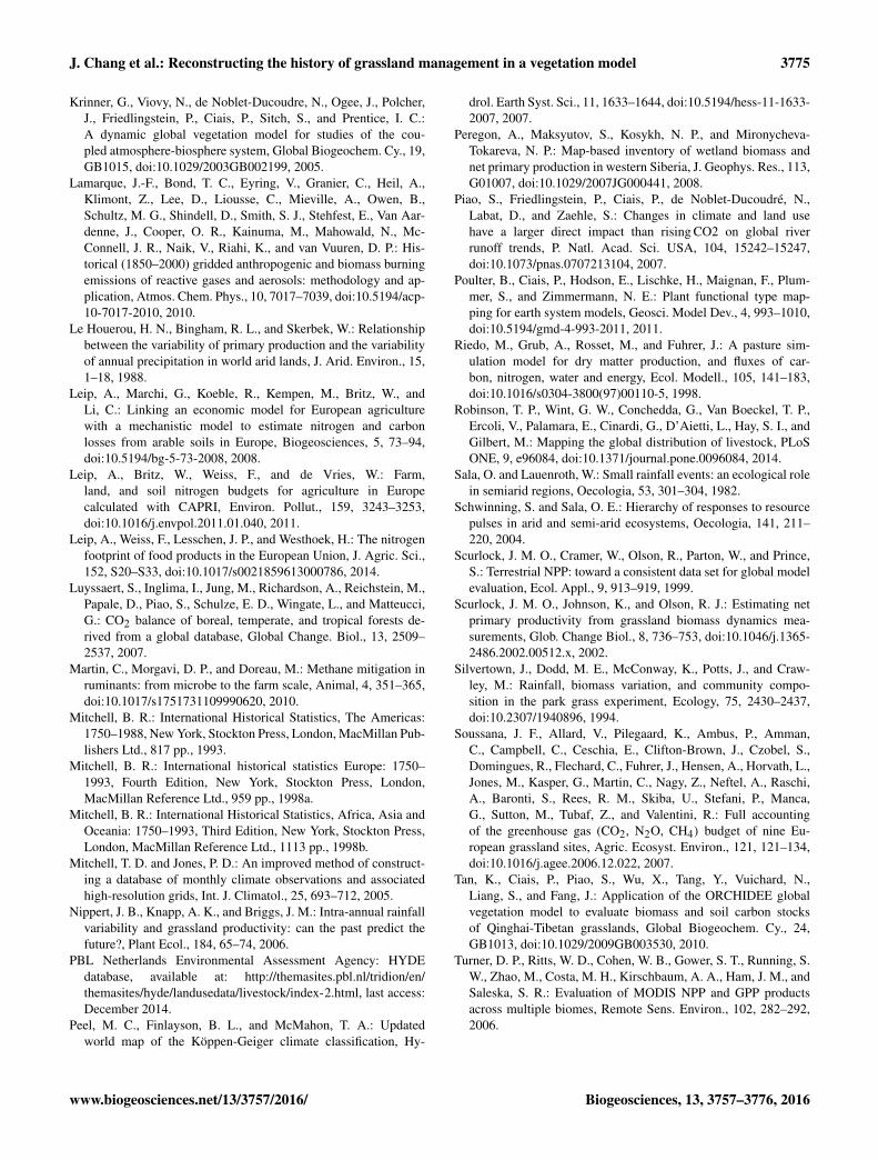
J. Chang et al.: Reconstructing the history of grassland management in a vegetation model 3775
Krinner, G., Viovy, N., de Noblet-Ducoudre, N., Ogee, J., Polcher,J., Friedlingstein, P., Ciais, P., Sitch, S., and Prentice, I. C.:A dynamic global vegetation model for studies of the cou-pled atmosphere-biosphere system, Global Biogeochem. Cy., 19,GB1015, doi:10.1029/2003GB002199, 2005.
Lamarque, J.-F., Bond, T. C., Eyring, V., Granier, C., Heil, A.,Klimont, Z., Lee, D., Liousse, C., Mieville, A., Owen, B.,Schultz, M. G., Shindell, D., Smith, S. J., Stehfest, E., Van Aar-denne, J., Cooper, O. R., Kainuma, M., Mahowald, N., Mc-Connell, J. R., Naik, V., Riahi, K., and van Vuuren, D. P.: His-torical (1850–2000) gridded anthropogenic and biomass burningemissions of reactive gases and aerosols: methodology and ap-plication, Atmos. Chem. Phys., 10, 7017–7039, doi:10.5194/acp-10-7017-2010, 2010.
Le Houerou, H. N., Bingham, R. L., and Skerbek, W.: Relationshipbetween the variability of primary production and the variabilityof annual precipitation in world arid lands, J. Arid. Environ., 15,1–18, 1988.
Leip, A., Marchi, G., Koeble, R., Kempen, M., Britz, W., andLi, C.: Linking an economic model for European agriculturewith a mechanistic model to estimate nitrogen and carbonlosses from arable soils in Europe, Biogeosciences, 5, 73–94,doi:10.5194/bg-5-73-2008, 2008.
Leip, A., Britz, W., Weiss, F., and de Vries, W.: Farm,land, and soil nitrogen budgets for agriculture in Europecalculated with CAPRI, Environ. Pollut., 159, 3243–3253,doi:10.1016/j.envpol.2011.01.040, 2011.
Leip, A., Weiss, F., Lesschen, J. P., and Westhoek, H.: The nitrogenfootprint of food products in the European Union, J. Agric. Sci.,152, S20–S33, doi:10.1017/s0021859613000786, 2014.
Luyssaert, S., Inglima, I., Jung, M., Richardson, A., Reichstein, M.,Papale, D., Piao, S., Schulze, E. D., Wingate, L., and Matteucci,G.: CO2 balance of boreal, temperate, and tropical forests de-rived from a global database, Global Change. Biol., 13, 2509–2537, 2007.
Martin, C., Morgavi, D. P., and Doreau, M.: Methane mitigation inruminants: from microbe to the farm scale, Animal, 4, 351–365,doi:10.1017/s1751731109990620, 2010.
Mitchell, B. R.: International Historical Statistics, The Americas:1750–1988, New York, Stockton Press, London, MacMillan Pub-lishers Ltd., 817 pp., 1993.
Mitchell, B. R.: International historical statistics Europe: 1750–1993, Fourth Edition, New York, Stockton Press, London,MacMillan Reference Ltd., 959 pp., 1998a.
Mitchell, B. R.: International Historical Statistics, Africa, Asia andOceania: 1750–1993, Third Edition, New York, Stockton Press,London, MacMillan Reference Ltd., 1113 pp., 1998b.
Mitchell, T. D. and Jones, P. D.: An improved method of construct-ing a database of monthly climate observations and associatedhigh-resolution grids, Int. J. Climatol., 25, 693–712, 2005.
Nippert, J. B., Knapp, A. K., and Briggs, J. M.: Intra-annual rainfallvariability and grassland productivity: can the past predict thefuture?, Plant Ecol., 184, 65–74, 2006.
PBL Netherlands Environmental Assessment Agency: HYDEdatabase, available at: http://themasites.pbl.nl/tridion/en/themasites/hyde/landusedata/livestock/index-2.html, last access:December 2014.
Peel, M. C., Finlayson, B. L., and McMahon, T. A.: Updatedworld map of the Köppen-Geiger climate classification, Hy-
drol. Earth Syst. Sci., 11, 1633–1644, doi:10.5194/hess-11-1633-2007, 2007.
Peregon, A., Maksyutov, S., Kosykh, N. P., and Mironycheva-Tokareva, N. P.: Map-based inventory of wetland biomass andnet primary production in western Siberia, J. Geophys. Res., 113,G01007, doi:10.1029/2007JG000441, 2008.
Piao, S., Friedlingstein, P., Ciais, P., de Noblet-Ducoudré, N.,Labat, D., and Zaehle, S.: Changes in climate and land usehave a larger direct impact than rising CO2 on global riverrunoff trends, P. Natl. Acad. Sci. USA, 104, 15242–15247,doi:10.1073/pnas.0707213104, 2007.
Poulter, B., Ciais, P., Hodson, E., Lischke, H., Maignan, F., Plum-mer, S., and Zimmermann, N. E.: Plant functional type map-ping for earth system models, Geosci. Model Dev., 4, 993–1010,doi:10.5194/gmd-4-993-2011, 2011.
Riedo, M., Grub, A., Rosset, M., and Fuhrer, J.: A pasture sim-ulation model for dry matter production, and fluxes of car-bon, nitrogen, water and energy, Ecol. Modell., 105, 141–183,doi:10.1016/s0304-3800(97)00110-5, 1998.
Robinson, T. P., Wint, G. W., Conchedda, G., Van Boeckel, T. P.,Ercoli, V., Palamara, E., Cinardi, G., D’Aietti, L., Hay, S. I., andGilbert, M.: Mapping the global distribution of livestock, PLoSONE, 9, e96084, doi:10.1371/journal.pone.0096084, 2014.
Sala, O. and Lauenroth, W.: Small rainfall events: an ecological rolein semiarid regions, Oecologia, 53, 301–304, 1982.
Schwinning, S. and Sala, O. E.: Hierarchy of responses to resourcepulses in arid and semi-arid ecosystems, Oecologia, 141, 211–220, 2004.
Scurlock, J. M. O., Cramer, W., Olson, R., Parton, W., and Prince,S.: Terrestrial NPP: toward a consistent data set for global modelevaluation, Ecol. Appl., 9, 913–919, 1999.
Scurlock, J. M. O., Johnson, K., and Olson, R. J.: Estimating netprimary productivity from grassland biomass dynamics mea-surements, Glob. Change Biol., 8, 736–753, doi:10.1046/j.1365-2486.2002.00512.x, 2002.
Silvertown, J., Dodd, M. E., McConway, K., Potts, J., and Craw-ley, M.: Rainfall, biomass variation, and community compo-sition in the park grass experiment, Ecology, 75, 2430–2437,doi:10.2307/1940896, 1994.
Soussana, J. F., Allard, V., Pilegaard, K., Ambus, P., Amman,C., Campbell, C., Ceschia, E., Clifton-Brown, J., Czobel, S.,Domingues, R., Flechard, C., Fuhrer, J., Hensen, A., Horvath, L.,Jones, M., Kasper, G., Martin, C., Nagy, Z., Neftel, A., Raschi,A., Baronti, S., Rees, R. M., Skiba, U., Stefani, P., Manca,G., Sutton, M., Tubaf, Z., and Valentini, R.: Full accountingof the greenhouse gas (CO2, N2O, CH4) budget of nine Eu-ropean grassland sites, Agric. Ecosyst. Environ., 121, 121–134,doi:10.1016/j.agee.2006.12.022, 2007.
Tan, K., Ciais, P., Piao, S., Wu, X., Tang, Y., Vuichard, N.,Liang, S., and Fang, J.: Application of the ORCHIDEE globalvegetation model to evaluate biomass and soil carbon stocksof Qinghai-Tibetan grasslands, Global Biogeochem. Cy., 24,GB1013, doi:10.1029/2009GB003530, 2010.
Turner, D. P., Ritts, W. D., Cohen, W. B., Gower, S. T., Running, S.W., Zhao, M., Costa, M. H., Kirschbaum, A. A., Ham, J. M., andSaleska, S. R.: Evaluation of MODIS NPP and GPP productsacross multiple biomes, Remote Sens. Environ., 102, 282–292,2006.
www.biogeosciences.net/13/3757/2016/ Biogeosciences, 13, 3757–3776, 2016

3776 J. Chang et al.: Reconstructing the history of grassland management in a vegetation model
Verheijen, L. M., Brovkin, V., Aerts, R., Bönisch, G., Cornelissen,J. H. C., Kattge, J., Reich, P. B., Wright, I. J., and van Bodegom,P. M.: Impacts of trait variation through observed trait-climate re-lationships on performance of an Earth system model: a concep-tual analysis, Biogeosciences, 10, 5497–5515, doi:10.5194/bg-10-5497-2013, 2013.
Viovy, N.: CRU-NCEPv4, CRUNCEP dataset, available at: http://dods.extra.cea.fr/data/p529viov/cruncep/readme.htm (last ac-cess: December 2013), 2013.
Viovy, N. and de Noblet, N.: Coupling water and Carbon cycle inthe biosphere, Sci. Géol. Bull., 50, 109–121, 1997.
Vuichard, N., Ciais, P., Viovy, N., Calanca, P., and Sous-sana, J.-F.: Estimating the greenhouse gas fluxes of Euro-pean grasslands with a process-based model: 2. Simulations atthe continental level, Global Biogeochem. Cy., 21, GB1005,doi:10.1029/2005GB002612, 2007a.
Vuichard, N., Soussana, J.-F., Ciais, P., Viovy, N., Ammann, C.,Calanca, P., Clifton-Brown, J., Fuhrer, J., Jones, M., and Mar-tin, C.: Estimating the greenhouse gas fluxes of European grass-lands with a process-based model: 1. Model evaluation fromin situ measurements, Global Biogeochem. Cy., 21, G01002,doi:10.1029/2004JG000004, 2007b.
Wang, T., Ottlé, C., Boone, A., Ciais, P., Brun, E., Morin, S., Krin-ner, G., Piao, S., and Peng, S.: Evaluation of an improved inter-mediate complexity snow scheme in the ORCHIDEE land sur-face model, J. Geophys. Res.-Atmos., 118, 6064–6079, 2013.
Warneck, P., Chemistry of the Natural Atmosphere, 757 pp., Aca-demic, San Diego, Calif., 1988.
Zeng, C., Wu, J., and Zhang, X.: Effects of grazing on above-vs. below-ground biomass allocation of alpine grasslands onthe northern Tibetan Plateau, PLoS ONE, 10, e0135173,doi:10.1371/journal.pone.0135173, 2015.
Zhang, Y., Yu, Q., Jiang, J., and Tang, Y.: Calibration ofTerra/MODIS gross primary production over an irrigated crop-land on the North China Plain and an alpine meadow on the Ti-betan Plateau, Glob. Change. Biol., 14, 757–767, 2008.
Zhao, M. and Running, S. W.: Drought-induced reduction in globalterrestrial net primary production from 2000 through 2009, Sci-ence, 329, 940–943, 2010.
Zhao, M., Heinsch, F. A., Nemani, R. R., and Running, S. W.: Im-provements of the MODIS terrestrial gross and net primary pro-duction global data set, Remote Sens. Environ., 95, 164–176,2005.
WorldClim: Global Climate Data, available at: http://www.worldclim.org/, last access: December 2014.
Biogeosciences, 13, 3757–3776, 2016 www.biogeosciences.net/13/3757/2016/