combining low-energy electrical resistance heating with biotic
TRANSCRIPT

FINAL REPORT Combining Low-Energy Electrical Resistance Heating
With Biotic and Abiotic Reactions for Treatment of Chlorinated Solvent DNAPL Source Areas
ESTCP Project ER-200719
December 2012
Tamzen Macbeth CDM Michael Truex Pacific Northwest National Laboratory Thomas Powell Thermal Remediation Services Mandy Michalsen United States Army Corps of Engineers

REPORT DOCUMENTATION PAGE Form Approved
OMB No. 0704-0188 Public reporting burden for this collection of information is estimated to average 1 hour per response, including the time for reviewing instructions, searching existing data sources, gathering and maintaining the data needed, and completing and reviewing this collection of information. Send comments regarding this burden estimate or any other aspect of this collection of information, including suggestions for reducing this burden to Department of Defense, Washington Headquarters Services, Directorate for Information Operations and Reports (0704-0188), 1215 Jefferson Davis Highway, Suite 1204, Arlington, VA 22202-4302. Respondents should be aware that notwithstanding any other provision of law, no person shall be subject to any penalty for failing to comply with a collection of information if it does not display a currently valid OMB control number. PLEASE DO NOT RETURN YOUR FORM TO THE ABOVE ADDRESS.
1. REPORT DATE (DD-MM-YYYY)
12-05-2012
2. REPORT TYPE
ESTCP Final Report
3. DATES COVERED (From - To)
June 2007 to December 2012
4. TITLE AND SUBTITLE
Combining Low-Energy Electrical Resistance Heating With Biotic
and Abiotic Reactions for Treatment of Chlorinated Solvent
DNAPL Source Area
5a. CONTRACT NUMBER
W912DQ-08-D-0018
5b. GRANT NUMBER
5c. PROGRAM ELEMENT NUMBER
6. AUTHOR(S)
Macbeth, Tamzen, W.
Truex, Michael, J.
Powell Thomas,
Michalsen, Mandy
5d. PROJECT NUMBER
ER-0719
5e. TASK NUMBER
W912DQ-08-D-0018-EC02
5f. WORK UNIT NUMBER
7. PERFORMING ORGANIZATION NAME(S) AND ADDRESS(ES)
CDM Smith
50 West 14th Street Suite 200
Helena, MT 59601
Pacific Northwest National Laboratory
P.O. Box 999, MS K6-96
Richland/WA 99352
Thermal Remediation Services
PO Box 737
Longview, WA 98632
Unites States Army Corps of Engineers
4735 East Marginal Way South
Seattle, WA 98134
8. PERFORMING ORGANIZATION REPORT NUMBER
9. SPONSORING / MONITORING AGENCY NAME(S) AND ADDRESS(ES) 10. SPONSOR/MONITOR’S ACRONYM(S)
Unites States Army Corps of
Engineers
4735 East Marginal Way South
Seattle, WA 98134
USACE
11. SPONSOR/MONITOR’S REPORT
NUMBER(S)
12. DISTRIBUTION / AVAILABILITY STATEMENT
UU
13. SUPPLEMENTARY NOTES

14. ABSTRACT
The effectiveness and timeframe of in situ remedies such as in situ bioremediation (ISB) and zero-valent iron (ZVI) is a function of mass
transfer when applied in chlorinated solvent dense nonaqueous phase liquid (DNAPL) source zones. The ESTCP ER-0719 project
demonstrated combining low-temperature subsurface heating with in situ remedies to enhance remediation performance through both
increased degradation reaction rates and contaminant dissolution. Dechlorination was induced in two test cells for ZVI and ISB. For the
ZVI test, increased temperature from 10oC to between 35 and 45
oC increased dechlorination by a factor of 4 to 8. For the ISB test,
increasing the temperatures (10oC to between 35 and 45
oC) accelerated overall contaminant dechlorination by a factor of 2-4 at hotspot
locations close to residual contaminant mass. Field test results demonstrated that moderate heating and minor operational costs enhanced
efficiency and effectiveness of in situ treatment of trichloroethene (TCE). Capture and treatment of contaminated vapor— a major cost
element of standard thermal treatment—was not needed as treatment maintained low aqueous TCE concentrations. Additional
infrastructure needed for heating was limited to subsurface electrodes and a power control unit. These results suggest that combined
heating and in situ treatment may be cost effective in source zones with moderate contaminant mass or when combined with high-
temperature thermal.
As expected, reductive dechlorination occurred with ISB and a mixture of reductive dechlorination and reductive elimination occurred with
ZVI. Increased reaction and contaminant dissolution were observed in both tests with increased temperature, but volatilization was
minimal during the test because in situ reactions maintained low aqueous phase TCE concentrations.
For the ISB test, increasing the temperatures (10oC to between 35 and 45
oC) accelerated overall contaminant dechlorination by a factor of
2-4 at hotspot locations close to residual contaminant mass. An average of 430 kW-h per day of electrical power was applied to raise the
test zone temperature to 40oC within 30 days over a volume of 271 m
3, after which, 25-140 kW-h per day was sufficient to sustain the
temperature depending on infiltration rates.
Field test results demonstrated that moderate heating and minor operational costs enhanced efficiency and effectiveness of in situ treatment
of TCE. Capture and treatment of contaminated vapor— a major cost element of standard thermal treatment—was not needed as treatment
maintained low aqueous TCE concentrations. Additional infrastructure needed for heating was limited to subsurface electrodes and a
power control unit. These results suggest that combined heating and in situ treatment may be cost effective in source zones with moderate
contaminant mass or when combined with high-temperature thermal.
15. SUBJECT TERMS
Chlorinated solvent, DNAPL, bioremediation, zero valent iron, thermal remediation, electrical
resistance heating, combined remedy
16. SECURITY CLASSIFICATION OF:
17. LIMITATION OF ABSTRACT
18. NUMBER OF PAGES
19a. NAME OF RESPONSIBLE PERSON
Tamzen W. Macbeth
a. REPORT
b. ABSTRACT
c. THIS PAGE
SAR
19b. TELEPHONE NUMBER (include area
code)
(208)904-0238
Standard Form 298 (Rev. 8-98) Prescribed by ANSI Std. Z39.18

ACKNOWLEDGEMENTS
The principal investigator (PI) for this project was Dr. Tamzen Macbeth, P.E. (CDM, Smith Inc.) along with Dr. Kent Sorenson, who provided technical oversight, and Howard Young led the overall development of the project and designed and implemented the in situ bioremediation. Co-PI Michael Truex with Pacific Northwest National Laboratory supported by Mart Oostrom, Lirong Zhong, Vince Vermeul, led the development of the zero valent iron (ZVI) design and implementation. Thomas Powell, also a Co-PI, supported by Gregory Sandberg and Chad Crownover, with Thermal Remediation Services led the design and operation of the low-energy heating system. North Wind, Inc., led by Saige Ballack-Dixon, performed most of the field work for the demonstration as well as the data management. This demonstration was funded entirely by ESTCP under project ER-0719. Their thoughtful reviews of project documents and their support significantly contributed to the success of the project. Special thanks are due to Andrea Leeson and Hans Stroo of the ESTCP program in this regard. The U.S. Army Corps of Engineers Seattle District was instrumental in providing support and coordinating with the Ft. Lewis Public Works Department. From the Corps, special thanks are extended to Kira Lynch (now with EPA Region 10), Mandy Michalsen, Richard Smith, Emile Petri, and Travis Shaw. From Ft. Lewis Public Works, Richard Wilson (now with the Corps, Seattle District) and James Gillie are due many thanks.

EXECUTIVE SUMMARY
The applicability of in situ groundwater remedies such as in situ bioremediation (ISB) or zero valent iron (ZVI) reduction in chlorinated solvent source zones (i.e. containing dense non-aqueous phase liquids [DNAPLs]) is often limited by the relatively long treatment timeframes required to meet remedial objectives at sites. Combining subsurface heating with in situ remedies can potentially accelerate the treatment rate by increasing dissolution of residual contaminants into groundwater where they are available for in situ degradation reactions. Conceptually, the goal of ESTCP demonstration project ER-0719 was to evaluate moderate heating (i.e. 35-50 oC) to accelerate dissolution/desorption of residual trichloroethylene (TCE) contamination offset by concomitant accelerated in situ degradation kinetics, and to minimize volatilization and the need for soil gas extraction and treatment, typically required for high-temperature thermal applications. This field demonstration combined electrical resistance heating with for both ZVI and ISB for TCE treatment.
The demonstration objectives included quantifying, 1) the effect of low-energy heating on the extent and rate of contaminant degradation reactions, 2) the enhanced mass removal rate, 3) the relative contribution of biotic and abiotic contaminant degradation mechanisms at different temperatures, and 4) the cost-benefit of applying low-energy heating with in situ treatments. The project was broken up into three phases. Phase 1 consisted of initial characterization and verification of the suitability of two test cells, in which ISB and ZVI to be demonstrated, to meet project objectives. Phase 2 consisted of a field demonstration of ISB and ZVI without heating to establish performance of the individual technologies including the degradation kinetics and mass balance factors at ambient temperature. Phase 3 consisted of a field demonstration of ISB with low-energy ERH to evaluate treatment performance at elevated temperatures of approximately 30-45°C, and ZVI at elevated temperatures of approximately 30-55°C. This field demonstration was used to evaluate the feasibility of various low-temperature heating applications for in situ treatment including: (1) application designs with low-temperature heating as the primary treatment, and (2) application designs with low-temperature heating in combination with high temperature heating in series and in parallel.
Phase 1 characterization included a soil gas survey, and confirmation soil and groundwater sampling which demonstrated high concentrations of TCE in soils (max. 220 mg/kg) and groundwater (max. 29 ppm) within the two test cells. Phase 2 was initiated with injection of zero-valent iron (ZVI) within the ZVI test cell. One of the most significant challenges to in situ ZVI reduction is effective distribution of ZVI particles within subsurface environments. During the ER-0719 field demonstration, micron-scale ZVI particles were suspended within a shear-thinning fluid to increase distribution of micron-scale ZVI. Approximately 190 kg of 2-micron-diameter ZVI particles were injected into the top six feet of an unconfined aquifer within the trichloroethene (TCE) source zone. Continuous monitoring during and after injection revealed ZVI concentrations at the monitoring wells at all wells within 12 feet at the end of the injection period. TCE dechlorination was monitored over a period of two months at the monitoring wells

and the injection well as part of validating ZVI particle distribution. All wells showed indications of dechlorination with only dechlorination products, with high concentrations of ethene and ethane, present by the end of two months at ambient temperature. Data indicate a mixture of abiotic reactions and biotic dechlorination reactions were occurring as daughter products also included cis-DCE (biotic) and ethene and ethane (abiotic).
For the ISB test cell, efficient degradation of TCE was established during Phase 2 via monthly injections of emulsified vegetable oil and powdered whey for nine months. A reactive treatment zone approximately 20 feet in diameter and 12 feet thick was established where geochemical conditions were generally reduced to support methane production and reductive dechlorination of TCE to primarily cis-DCE with trace ethene was achieved at ambient temperature. However, relatively high groundwater velocities within the treatment zone resulted in relatively low retention of amendment within the test cell, which was the reason that monthly injections were conducted.
Electrical resistance heating was applied to raise the temperature in the test zone to between 30oC and 45oC in the ISB test cell and to 40oC and 55oC in the ZVI test cell. The elevated temperatures increased the dissolution of contaminant into the groundwater and increased the rate and extent of dechlorination in both test cells. The viability of moderately-heated in situ treatment requires that increases in physical mass transfer rates for both dissolution and volatilization as temperatures increase must be balanced by contaminant degradation to prevent transport of mobilized contaminants out of the heated treatment zone. Contaminant dissolution and volatilization generally increase with increasing temperature. Imhoff et al., 1997 empirically and predictively reported that moderate temperature increases during hot water flushing for chlorinated solvent treatment enhance the mass transfer rate of residual DNAPL by a factor of 4 to 5 when temperatures were increased from 5oC to 60oC. Similarly, total contaminant mass discharge observed during the ER-0719 demonstration increased by a factor of 4-16 within the ZVI test cell at approximately 45oC compared to ambient temperatures of 10oC. This enhanced mass transfer was evaluated largely based on reductive daughter products as the degradation kinetics were sufficiently high to keep TCE concentration low. For the ISB test cell, total contaminant mass discharge increased by a factor of approximately 4-5 at approximately 40oC compared to ambient temperatures of 10oC. The fraction of ethene dramatically increased during Phase3 compared to Phase 2. A longer reactive zone was required downgradient of the ISB DNAPL zone to ensure complete biodegradation of contaminants transported from the heated zone. In addition, contaminant fluxes to the vadose zone increased by less than 1.5% at the elevated temperatures compared to ambient indicating VOC losses to the vadose zone were minimal.
A summary of cost factors for low-temperature ZVI and ISB suggest that low-temperature heating is less expensive than high temperature ERH, but only incrementally so. Therefore, application of low-temperature heating likely makes sense only for sites that contain only low to moderate VOC concentrations as residual in soil where contaminant mass could be removed in less than 1-2 years. However, the benefit of heating to in situ reactions was clearly demonstrated

both from an enhanced kinetics of degradation reactions and VOC mass removal rates. Therefore, combining in situ treatment with heating, especially for sites already considering high temperature heating, may provide added benefit. In addition, in situ technologies could be implemented after thermal shut down to treat any remaining contaminants in the treatment zone.

i ESTCP ER-0719 Final Report
TABLE OF CONTENTS
ACKNOWLEDGEMENTS
EXECUTIVE SUMMARY
ACRONYMS AND ABBREVIATIONS .................................................................... viii SECTION 1 INTRODUCTION ..................................................................................... 1
1.1 Background .............................................................................................................. 1 1.2 Objective of the Demonstration ............................................................................... 3 1.3 Regulatory Drivers ................................................................................................... 4 1.4 Stakeholders/End-User Issues .................................................................................. 4
SECTION 2 TECHNOLOGY DESCRIPTION ........................................................... 7 2.1 Low-Energy ERH .................................................................................................... 7 2.2 In Situ Bioremediation ............................................................................................. 7 2.3 ZVI Technology ..................................................................................................... 12 2.4 Advantages and Limitation of the Technology ...................................................... 15
SECTION 3 PERFORMANCE OBJECTIVES ......................................................... 19
SECTION 4 SITE DESCRIPTION ............................................................................. 21 4.1 Site Location and History ...................................................................................... 21 4.2 Site Geology/Hydrogeology .................................................................................. 21
4.2.1 Geology ......................................................................................................... 21 4.2.2 Hydrogeology ................................................................................................ 22
4.3 Contaminant Distribution ....................................................................................... 23
SECTION 5 TEST DESIGN ........................................................................................ 29 5.1 Conceptual Experimental Design........................................................................... 29 5.2 Phase 1: Baseline Characterization ........................................................................ 30
5.2.1 Gore™ Sorber Survey ................................................................................... 31 5.2.2 Soil Characterization and Installation of ISB Test Cell Wells ...................... 34 5.2.3 Soil Characterization and Installation of ZVI Test Cell Wells ..................... 39 5.2.4 Hydraulic Characterization: ISB Test Cell.................................................... 40
Tracer Test Design ........................................................................................................................................... 40 Hydraulic Testing Results ............................................................................................................................ 43 Groundwater Velocity .................................................................................................................................... 43 Hydraulic Conductivity .................................................................................................................................. 50
5.2.5 Hydraulic Characterization: ZVI Test Cell ................................................... 51 5.3 Laboratory Study Results ....................................................................................... 51 5.4 Design and Layout of Technology Components.................................................... 52
5.4.1 ISB Field Test Design ................................................................................... 52 ISB Test Cell Layout ........................................................................................................................................ 52 ISB Field Injection Equipment .................................................................................................................... 53
5.4.2 ZVI Field Test Design ................................................................................... 53 ZVI Test Cell Layout ........................................................................................................................................ 53

Table of Contents
ii
ESTCP ER-0719 Final Report
ZVI Injection Equipment ............................................................................................................................... 55 5.4.3 ERH System Design ...................................................................................... 55
ERH Power Control Unit ............................................................................................................................... 55 ERH Electrode Layout .................................................................................................................................... 59 Temperature Monitoring Points ............................................................................................................... 63
5.5 Field Testing .......................................................................................................... 64 5.5.1 Phase 2 and 3: ISB Injection Strategy ........................................................... 64
EOS® Injections ................................................................................................................................................. 64 Bicarbonate Buffered Whey Injections .................................................................................................. 66
5.5.2 Phase 2 and 3: ZVI Injection Strategy .......................................................... 66 5.5.3 Phase 3: ERH System Operations ................................................................. 67
ERH System Start Up ...................................................................................................................................... 67 Safety and Security .......................................................................................................................................... 71 ERH Operations ................................................................................................................................................ 71 ERH Operations System Optimization .................................................................................................... 72 Demobilization .................................................................................................................................................. 72
5.6 Sampling Methods ................................................................................................. 72 5.6.1 Tracer Test..................................................................................................... 75 5.6.2 Groundwater Sampling Methods .................................................................. 78 5.6.3 Soil Gas Sampling Methods .......................................................................... 78 5.6.4 Soil Sampling Methods ................................................................................. 79 5.6.5 EEH Sampling Methods ................................................................................ 79
Subsurface Temperature Monitoring ...................................................................................................... 79 ERH Power Output and Control Monitoring ........................................................................................ 79
5.7 Sampling Results ................................................................................................... 80 5.7.1 Phases 2 and 3: ISB ....................................................................................... 80
5.7.1.1 Groundwater Monitoring .......................................................................................................... 81 Mass Flux And Discharge Modeling ......................................................................................................... 93 5.7.1.2 Soil Vapor Monitoring .............................................................................................................. 101
5.7.2 ZVI Injection Results .................................................................................. 111 5.7.3 Phase 2 and 3: ZVI ...................................................................................... 116
Groundwater Monitoring .......................................................................................................................... 116 Geochemical Response ............................................................................................................................... 116 Contaminant And Dechlorination Product Concentrations ....................................................... 119 Soil Vapor Monitoring ................................................................................................................................. 130 Soil Monitoring ............................................................................................................................................... 130 Microbial Community.................................................................................................................................. 132
5.7.4 Phase 3: Low-Energy ERH ......................................................................... 132 Power and Energy......................................................................................................................................... 132 Temperature ................................................................................................................................................... 136
SECTION 6 PERFORMANCE ASSESSMENT ...................................................... 144 6.1 Mass Balance Factors ISB ................................................................................... 146
6.1.1 ISB Enhanced Mass Transfer ...................................................................... 146 6.1.2 ISB Impact of Elevated Temperature on Kinetics ...................................... 148
6.2 Mass Balance Factors ZVI ................................................................................... 151

Table of Contents
iii ESTCP ER-0719 Final Report
6.2.1 ZVI Mass Transfer ...................................................................................... 151 6.2.2 ZVI Kinetic Changes ................................................................................... 154 6.2.3 Biotic/Abiotic .............................................................................................. 155 6.2.4 Impact of Temperature on Dissolution/Volatilization ................................ 156
6.3 Summary of Performance related to Objectives .................................................. 157
SECTION 7 COST ASSESSMENT ........................................................................... 160 7.1 Cost Model ........................................................................................................... 160
7.1.1 “Summary Info ZVI-Thermal” Worksheet ................................................. 164 Start-Up Costs ................................................................................................................................................. 165 Capital Costs .................................................................................................................................................... 166 Operation And Maintenance Costs ........................................................................................................ 166 Demobilization Costs ................................................................................................................................... 166 Waste Disposal Costs ................................................................................................................................... 167 Grand Total Combined ZVI-Thermal Costs for this Demonstration ....................................... 167
7.1.2 “Summary Info Bio-Thermal” Worksheet .................................................. 167 Start-Up Costs ................................................................................................................................................. 167 Capital Costs .................................................................................................................................................... 167 Operation and Maintenance Costs ......................................................................................................... 167 Demobilization Costs ................................................................................................................................... 168 Waste Disposal Costs ................................................................................................................................... 168 Grand Total Combined ISB-Thermal Costs For This Demonstration ..................................... 168
7.1.3 “Summary Info Thermal” Worksheet ......................................................... 168 7.2 Cost Drivers ......................................................................................................... 168
7.2.1 ZVI .............................................................................................................. 168 7.2.2 ISB ............................................................................................................... 170 7.2.3 Thermal .................................................................................................... 171
7.3 Cost Analysis ....................................................................................................... 171
SECTION 8 IMPLEMENTATION ........................................................................... 172 8.1 Key Regulations ................................................................................................... 174 8.2 Other Regulatory Issues ....................................................................................... 174 8.3 End-User Issues ................................................................................................... 175 8.4 Procurement ......................................................................................................... 175
SECTION 9 REFERENCES ...................................................................................... 176
LIST OF FIGURES Figure 2-1. Areal view of Ft. Lewis EGDY and location of demonstration test cells ....... 8 Figure 2-2. Potential reactions during ISB ........................................................................ 9 Figure 2-3. Potential reactions with ZVI ......................................................................... 10 Figure 2-4. Preliminary data from Ft. Lewis show that DHC might have an optimal
temperature range for growth that is well above typical ambient groundwater. ................................................................................................ 11

Table of Contents
iv
ESTCP ER-0719 Final Report
Figure 2-5. Ft. Lewis NAPL Area 3 data showing the response of DHC and functional reductase genes tceA, bvcA, and vcrA on increasing temperature during thermal heating during the ERH remedy ..................................................... 13
Figure 4-1. Treated Sites in Relation to EGDY Site Features ......................................... 24 Figure 4-2. Test Site Existing Sample Locations and Results ......................................... 26 Figure 4-3. Results of Membrane Interface Probe data collected during the RI at SM0030
located at the corner of EGDY Treatment Plant .......................................... 27 Figure 5-1. Schematic of emplaced Gore™ Sorber ......................................................... 32 Figure 5-2. Gore™ Sorber deployment locations ............................................................ 33 Figure 5-3. TCE Gore™ Sorber results ISB test cell ....................................................... 35 Figure 5-4. TCE Gore™ Sorber results ZVI test cell ...................................................... 37 Figure 5-5. Final Placement of ISB and ZVI Test Cells .................................................. 38 Figure 5-6. Breakthrough curve ISB-MW1 ..................................................................... 46 Figure 5-7. Breakthrough curve ISB-MW2 ..................................................................... 47 Figure 5-8. Breakthrough curve ISB-MW3 ..................................................................... 48 Figure 5-9. Breakthrough curves for ISB-MW4, ISB-MW5, ISB-MW6 ........................ 49 Figure 5-10. ZVI test cell well layout. The large circle shows the nominal target 3.5 m
injection radius ............................................................................................. 54 Figure 5-11. Test equipment schematic ........................................................................... 56 Figure 5-12. ZVI Injection System .................................................................................. 57 Figure 5-13. Power Control Unit (PCU) Electrical One-Line Drawing .......................... 58 Figure 5-14. ERH Electrode Locations of the ISB Test Cell ........................................... 60 Figure 5-15. ERH Electrode Locations of the ZVI Test Cell .......................................... 61 Figure 5-16. Electrode Detail ........................................................................................... 62 Figure 5-17. Stock solution of SlurryPro™ (0.2 wt%) .................................................... 68 Figure 5-18. Picture of ZVI injection solution during injection ...................................... 69 Figure 5-19. Samples at monitoring wells a the mid-point of ZVI injection ................... 70 Figure 5-20. Concentrations of carbon during Phase 1, 2 and 3 in the ISB wells Vertical
black lines indicate transition from Phase 2 to Phase 3 ............................... 84 Figure 5-21. Typical progression of redox parameters during Phase 2 and 3 ................. 87 Figure 5-22. Phase 2 and 3 total molar VOC mass in ISB test cell (A) and downgradient
concentration at ISB-MW4 (B) .................................................................... 90 Figure 5-23. Chlorine numbers calculated for wells ISB-INJ, ISB-MW1 through-MW3
(average of depths 12, 17, and 22 ft bgs) and downgradient wells ISB-MW4 through –MW6 during the demonstration.................................................... 92
Figure 5-24. Phase 2 and 3 total VOC mass flux (A), reductive daughter product mass flux (B) and VOC, daughter product and chloride discharge (C) as a function of temperature across the ISB-MW1 and ISB-MW2 transect ....... 94
Figure 5-25. MVS-modelled mass flux and discharge versus temperature from the ISB test cell at three timepoints during Phase 2 and 3 ........................................ 97
Figure 5-26. Results of molecular DNA Analysis for DHC during Phase 1, 2 and 3 of operations ................................................................................................... 101
Table of Contents
v ESTCP ER-0719 Final Report
Figure 5-27. TCE vapor flux during Phases 1, 2, and 3 for the ISB test cell ................ 104 Figure 5-28. cis-DCE vapor flux during Phases 1, 2, and 3 for the ISB test cell .......... 105 Figure 5-29. VC vapor flux during Phases 1, 2, and 3 for the ISB test cell .................. 106 Figure 5-30. Modeled and extrapolated vapor flux at 7 feet bgs in the ISB test cell .... 109 Figure 5-31. Modeled and extrapolated vapor flux at ground surface in the ISB test cell
.................................................................................................................... 110 Figure 5-32. Summary of soil concentration results for Phases 1, 2 and 3 for the ISB test
cell .............................................................................................................. 113 Figure 5-33. Pressure response at A) the injection well, B) monitoring well MW1 located
at a radial distance of 1.22 m from the injection well, and C) monitoring well MW5 located at a radial distance of 2.23 m from the injection well . 114
Figure 5-34. Water level variation during the field test ................................................. 117 Figure 5-35. Oxidation-reduction potential over time in the test cell ............................ 118 Figure 5-36. Measured pH response during ZVI demonstration (A) and for first 150 days
(B) .............................................................................................................. 120 Figure 5-37. Groundwater concentrations at well INJ. B graph presents groundwater
constituents at a refined scale to show details ........................................... 121 Figure 5-38. Groundwater concentrations at well MW1. B graph presents groundwater
constituents at a refined scale to show details ........................................... 122 Figure 5-39. Groundwater concentrations at well MW2. B graph presents groundwater
constituents at a refined scale to show details ........................................... 123 Figure 5-40. Groundwater concentrations at well MW3 ............................................... 124 Figure 5-41. Groundwater concentrations at well MW4 ............................................... 124 Figure 5-42. Groundwater concentrations at well MW ................................................. 125 Figure 5-43. Groundwater concentrations at well MW6 ............................................... 125 Figure 5-44. Groundwater concentrations at well MW7 B graph presents groundwater
constituents at a refined scale to show details ........................................... 126 Figure 5-45. Groundwater concentrations at well MW8. B graph presents groundwater
constituents at a refined scale to show details ........................................... 127 Figure 5-46. Groundwater concentrations at well MW9. B graph presents groundwater
constituents at a refined scale to show details ........................................... 128 Figure 5-47. Soil concentrations of TCE, DCE, and VC measured before ZVI treatment
and at the end of Phase 2, and Phase 3 ...................................................... 131 Figure 5-48. Microbial data during ZVI field test for functional genes (bvcA, vcrA,
tceA), and 16S RNA gene copies (16s) as a function of temperature Figure 5-49. Cumulative Energy Applied to the ZVI and ISB Test Cells ........... 133
Figure 5-50. Cumulative Energy and Temperature in ZVI and ISB Test Cells ............ 135 Figure 5-51. Weekly Energy Applied to the ZVI Test Cell ........................................... 137 Figure 5-52. Weekly Energy Applied to the ISB Test Cell ........................................... 138 Figure 5-53. Average Internal ZVI Test Cell TMP Temperatures ................................ 139 Figure 5-54. Average External ZVI Test Cell TMP Temperatures ............................... 140 Figure 5-55. Average Internal ISB Test Cell TMP Temperatures ................................. 142

Table of Contents
vi
ESTCP ER-0719 Final Report
Figure 5-56. Average External ISB Test Cell TMP Temperatures ................................ 143 Figure 6-1. Mass discharge analysis configuration where MDin is the influent mass
discharge and MDout-w and MDout-v are the effluent mass discharge in the water and vapor phases, respectively (Truex et al. 2011). ......................... 145
Figure 6-2. Linear correlation between MDdissolution, R, and Rtc as a function of temperature ................................................................................................ 149
Figure 6-3. Calculated TCE reaction rates and Nd for the INJ segment (Truex etal. 2011).................................................................................................................... 152
Figure 6-4. Chloride concentration over time in the ZVI test cell. Wells MW8 and MW9 are outside the injection zone, although a small amount of ZVI was distributed to MW8 during injection (Truex et al. 2011) ........................... 156
Figure 7-1. ZVI cost model treatment area and system infrastructure Figure 7-2. ISB cost model treatment area and system infrastructure ................................. 161
Figure 7-3. Treatment time comparison......................................................................... 165
LIST OF TABLES Table 1-1. Safe Drinking Water Act maximum contaminant levels for Ft. Lewis EGDY
contaminants of concern (COCs). ................................................................... 5
Table 5-1. Summary of ER-0719 Phase 1: Pre-Design Characterization/Baseline Activities. ...................................................................................................... 31
Objective 31
Table 5-2. Summary of Baseline Analytical Results from Field Screening and Soil Sampling. ....................................................................................................... 36
Table 5-3. Groundwater Flow Direction and Horizontal Hydraulic Conductivity at the ISB Test Cell ........................................................................................................ 40
Table 5-4. ISB Tracer injection strategy. ........................................................................ 41
Table 5-6. Groundwater elevations during and after ISB tracer test .............................. 44
Table 5-7. Hydraulic parameters calculated based on the tracer test and used for calculations. ................................................................................................... 45
Table 5-8. Estimated ZVI injection based on laboratory measured stoichiometry of TCE degraded per ZVI mass. ................................................................................. 52
Table 5-9. Concentration ratios for TCE and ZVI in laboratory tests compared to the selected ZVI injection for the field test. ........................................................ 52
Table 5-10. Details of completed wells within ISB test cell. .......................................... 53
Table 5-11. ZVI TMP Thermocouple Numbers and Depths. .......................................... 63
Table 5-12. ISB TMP Thermocouple Numbers and Depths. .......................................... 64
Table 5-13. Summary of amendment injections in the ISB test cell during Phase 2 and 3. ....................................................................................................................... 65
Table 5-14. ZVI Sample Types and Quantities. .............................................................. 73
Table 5-15. ISB Sample Types and Quantities. .............................................................. 75
Table of Contents
vii ESTCP ER-0719 Final Report
Table 5-16. Groundwater Sample Analysis Summary. ................................................... 77
Table 5-17. ERH Temperature and Power Sampling Frequency. ................................... 80
Table 5-18. Concentration of COD during baseline and post-Phase 2 EOS and whey injections. ...................................................................................................... 82
Table 5-19. Concentration of COD during Phase 2 and 3. .............................................. 83
Table 5-20. Summary of mass discharge estimates for Phase 2 and 3. .......................... 99
Table 5-21. TCE and Temperature Profiles for ISB-MW1. .......................................... 103
Table 5-22. Modeled Results for TCE for ISB-MW1. .................................................. 103
Table 5-23. Summary of tracer arrival and ZVI distribution results. ........................... 112
Table 5-24. Summary of ZVI injection parameters. ..................................................... 112
Table 5-25. Average groundwater concentration of TCE and dechlorination products.130
Table 6-1. Comparison of mass discharge from the ISB test cell in groundwater and in soil gas. ........................................................................................................ 147
Table 6-2. Average overall rate of TCE transformation based on organic dechlorination products (Rt) and chloride concentrations (Rtc) (Truex et al. 2011). ........... 155
Table 6-3. Summary of Achievement of Demonstration Performance Objectives. ...... 157
Table 7-1. Cost Assumption Model. ............................................................................. 160
APPENDICES Appendix A Points of Contact Appendix B Boring Logs Appendix C Laboratory Test Report Appendix D Analytical Data

Table of Contents
viii
ESTCP ER-0719 Final Report
ACRONYMS AND ABBREVIATIONS AFB Air Force Base ARD anaerobic reductive dechlorination bgs below ground surface oC degree Celcius CERCLA Comprehensive Environmental Response, Compensation, and Liability
Act CFR Code of Federal Regulations CMT continuous multi-channel tubing COC contaminant of concern COD chemical oxygen demand DCE dichloroethene DHC Dehalococcoides spp. DNA deoxyribonucleic acid DNAPL dense non-aqueous phase liquid DO dissolved oxygen DoD U.S. Department of Defense EGDY East Gate Disposal Yard (Fort Lewis) EOS® emulsified oil substrate EPA U.S. Environmental Protection Agency ERH electrical resistance heating ESTCP Environmental Security Technology Certification Program ft feet gpm gallons per minute ISB in situ bioremediation JBLM Joint Base Lewis-McChord kW kilowatt kWh kilowatt hour LOTO Lock-Out/Tag-Out µg microgram µg/kg microgram per kilogram µg/L microgram per liter MBAC Methanobacteriales MCOC Methanococcales mg/L milligram per liter MCRF Molecular Core Research Facility MMIC Methanomicrobiales mmol millimole MROD Mount Rainer Ordnance Detail MSAR Methanosarcina msl mean sea level MVS Mining Visualization System

Table of Contents
ix ESTCP ER-0719 Final Report
MW monitoring well NAPL non-aqueous phase liquid O&M operations and maintenance ORP oxidation-reduction potential PCE tetrachloroethene PCU power control unit PID photoionization detector ppm parts per million PVC polyvinyl chloride POL petroleum, oils, and lubricants PPE personal protective equipment qPCR quantitative polymerase chain reaction RCRA Resource Conservation and Recovery Act RI remedial investigation SV soil vapor TCA 1,1,1-trichloroethane TCE trichloroethene TMP temperature monitoring point TOC total organic carbon TRS Thermal Remediation Services UIC underground injection control uM micromoles per liter USACE United States Army Corps of Engineers USCS Unified Soils Classification System VC vinyl chloride VFA volatile fatty acid VOA volatile organic analysis VOC volatile organic compound WAC Waste Acceptance Criteria WDOE Washington Department of Ecology ZVI zero valent iron


1 ESTCP ER-0719 Final Report
SECTION 1 INTRODUCTION This report describes results of a field demonstration combining low energy electrical resistance heating (ERH) with in situ bioremediation (ISB), or with iron-based reduction using zero valent iron (ZVI), for the remediation of dense non-aqueous phase liquid (DNAPL) source zones. The field demonstration was conducted at Joint Base Lewis-McChord (JBLM) Landfill 2, formerly known as the Fort Lewis East Gate Disposal Yard (EGDY). The demonstration is focused on illustrating the benefits of combining low-energy ERH with either ISB or with iron-based reduction using injectable ZVI. This effort includes assessing the extent to which contaminant degradation is enhanced during heating compared to ambient temperatures, the relative contribution of biotic and abiotic contaminant degradation mechanisms at different temperatures, and the cost-benefit of applying low-energy heating with in situ treatments. The demonstration was conducted in three phases to allow accurate evaluation of the effects of ERH on ISB and ZVI reduction. The ISB and ZVI tests were conducted in hydraulically isolated test cells in the following three phases:
Phase 1: Pre-characterization and verification of the suitability of each test cell to meet demonstration objectives, treatment system installation, and baseline sampling.
Phase 2: Field demonstration of ISB and ZVI (without low-energy ERH).
Phase 3: Field demonstration of ISB and ZVI (with low-energy ERH).
The remainder of Section 1 briefly discusses background information, overall demonstration objectives, regulatory drivers, and stakeholder/end-user issues. The technologies are described in Section 2 and performance objectives are described in Section 3. Site conditions are described in Section 4. A detailed description of the technology demonstration design is presented in Section 5. The performance assessment strategy is described in Section 6. The cost assessment and implementation issues are addressed in Sections 7 and 8, respectively.
1.1 Background Chlorinated solvents are the most prevalent contaminants detected at hazardous waste sites according to the U.S. Environmental Protection Agency (EPA) National Priorities List. The U.S. Department of Defense (DoD) alone has approximately 3,000 sites contaminated with chlorinated solvents, with a large percentage of these sites containing residual sources of contamination containing DNAPLs, which serve as continuing, long-term sources of dissolved phase groundwater contamination.
The prevalence of chlorinated solvents has been linked to both to their widespread use and to their longevity in the environment. Their longevity is partly due to the hydrophobic nature that makes them such good solvents, as well as their relatively oxidized states that prevent them from serving as electron donors for microorganisms. Pertinent to their longevity is the fact that the solubility of the common chlorinated solvents (i.e., tetrachloroethene (PCE), trichloroethene (TCE), 1,1,1-trichloroethane (TCA), and carbon tetrachloride) ranges from about 200 to 1,400
Section 1 • Introduction
2
ESTCP ER-0719 Final Report
milligram per liter (mg/L) at 25°C (Sale 1998). These relatively low solubilities play a significant role in limiting mass transfer to the aqueous phase once the solvents contaminate groundwater. Dissolution of a DNAPL into groundwater is governed by the difference between the aqueous solubility of the compound and the actual concentration in groundwater. At typical groundwater velocities, the aqueous concentration of the solvent in the immediate vicinity of the groundwater non-aqueous phase liquid (NAPL) interface approaches the solubility within the first few centimeters of the DNAPL (Bouwer and McCarty 1983). Due to the laminar flow nature of most groundwater systems, very little mixing of water occurs, even a few centimeters from the DNAPL; thus, there is limited dissolution of DNAPLs into groundwater. The result is that chlorinated solvents can persist in groundwater for many decades.
The prevalence of DNAPL sites has prompted the DoD’s Strategic Environmental Research and Development Program (SERDP) and Environmental Security Technology Certification Program (ESTCP) program to develop a technical review panel focused on developing the strategy for research, and ultimately development of cost-effective technologies, to treat these sites. In particular, ESTCP has recognized a fundamental need for assessment of source zone treatment technologies focused on better implementation of existing technologies. Three relatively mature technologies, namely enhanced ISB, in situ iron-based reduction using ZVI, and thermal treatment using ERH, have been demonstrated independently for residual source zones. In situ technologies destroy contaminants without generation of secondary waste streams, are non-hazardous to workers and the environment, have relatively low capital and maintenance costs, and generally minimize disturbance of the site.
The remedial timeframe using many in situ technologies, however, is relatively long due to limitations in mass transfer of contaminants from the residual to the dissolved phase, where contaminants are available for destruction. Thermal treatment through ERH, which is a proven aggressive technology for the treatment of DNAPL source zones, rapidly removes large quantities of residual mass from subsurface environments. However, high capital and maintenance costs and the requirement for vapor control and secondary waste treatment make this technology a high cost alternative at many contaminated sites. Combining in situ and thermal treatment may provide many of the benefits of the in situ treatments with the shorter remedial timeframe associated with thermal treatment. This proposal is focused on demonstrating the benefits of combining low-energy ERH with either ISB or with iron-based reduction using injectable ZVI, including the assessment of the extent to which contaminant degradation is enhanced during heating compared to ambient temperatures, the relative contribution of biotic and abiotic contaminant degradation mechanisms at different temperatures, and the cost-benefit of applying low-energy heating with in situ treatments.
In providing thermally enhanced ISB or ZVI treatment, dissolution of DNAPL would be enhanced by the following phenomena:
1. At elevated temperatures, the dissolution rate of DNAPL is increased compared to lower temperatures. Dissolution of DNAPL is proportional to the diffusion rate in the water film. Because diffusion rate increases with temperature, so does the dissolution rate. For the

Section 1 • Introduction
3 ESTCP ER-0719 Final Report
proposed technology, it is important to maximize dissolution of DNAPL while minimizing volatilization so that the contaminants are transferred and maintained in the aqueous phase (where in situ reactions occur),but not transferred to the gas phase (where they must be captured to avoid spread of contamination).
2. At elevated temperatures, the desorption rate is increased compared to lower temperatures. An increase in temperature will enhance the rate of contaminant desorption and thereby improve the availability of these contaminants for degradation.
Although ERH, ISB, and ZVI are relatively mature technologies, the benefits of combining these technologies have not been fully demonstrated or validated. The overall cost for a combined system will be significantly lower than the cost for standard ERH because of the utilization of a low-energy system. Additionally, combining technologies will make in situ contaminant destruction reactions more effective for source area treatment. This combined technology approach is expected to provide more rapid source area cleanup than the ambient temperature in situ technologies alone but without the high cost of conventional ERH associated with boiling the entire water column and extracting and treating contaminants at the surface.
1.2 Objective of the Demonstration This demonstration is designed to evaluate the benefits of combining low-energy ERH with either ISB or with iron-based reduction using injectable ZVI. To evaluate the potential for decreased costs and increased efficiency of the combined remedies, the specific technical objectives of this demonstration are as follows:
Objective 1: To validate the rate and extent to which contaminant degradation is increased during enhanced ISB at a temperature of approximately 30 to 40°C compared to ISB at ambient temperature.
Objective 2: To validate the rate and extent to which contaminant degradation is increased during iron-based reduction at a temperature of approximately 50 to 60°C compared to ambient temperature.
Objective 3: To determine the relative contributions of biotic and abiotic degradation at different temperatures in order to optimize each.
Objective 4: To use data collected from a controlled field demonstration at a DoD site to develop cost and performance data for the combined remedies.
The goal of using heating to enhance in situ reactions is to treat a source area more cost effectively than is possible with only heating (e.g., ERH) or only an in situ remediation technology (e.g., ISB). A key data need for determining how to meet this goal is in finding the “sweet spot” where the cost of heating is more than offset by the gains in treatment efficiency for the in situ remediation technology. The demonstration provided a controlled field setting to test the impact of increased temperature on treatment efficiency using these in situ technologies. The demonstration also provided key engineering data relative to how ERH can be cost-effectively

Section 1 • Introduction
4
ESTCP ER-0719 Final Report
designed and applied to provide moderate heating rather than the standard design for heating to the boiling point.
1.3 Regulatory Drivers As stated in Section 1.1, chlorinated solvents are the most prevalent contaminants detected at hazardous waste sites, with the DoD alone having an estimated 2,151 sites with volatile organic compound (VOC) contamination in groundwater, with an estimated 85% of these sites containing residual sources (e.g., DNAPL) of contamination (EPA 2004). As stated previously, the solubilities of the common chlorinated solvents (PCE, TCE, TCA, and carbon tetrachloride) range from about 200 to 1,400 mg/L at 25°C (Sale 1998). These solubilities exceed Federal Safe Drinking Water Act maximum contaminant levels (see Table 1-1) by five to six orders of magnitude. The persistence of chlorinated solvents in groundwater, their prevalence, and their solubilities far in excess of health-based levels drive the need for cost-effective remediation technologies.
1.4 Stakeholders/End-User Issues This demonstration involves technologies (i.e., ISB, ZVI injections, and ERH) that are generally well received by the regulators and the public for many reasons. There are many advantages to the technologies (outlined in Section 2.4), including lower overall risks, low secondary waste generation, lower cost, and minimal impacts during operation.
There are several additional issues of concern to stakeholders/end-users specifically related to the use of thermally-enhanced treatments, including:
1. How will the application of heat affect the performance of ISB and ZVI?
2. Can the thermal systems be designed to minimize volatilization of contaminants such that in situ treatment is effective at treating released contaminant mass?
3. Is low-temperature heating cost-effective relative to implementing ZVI and ISB at ambient temperature?
The sampling and analysis strategy includes monitoring the ZVI and ISB at ambient and at elevated temperature. Potential risks posed by increased contaminant flux due to increased groundwater temperatures will be mitigated by the concomitant increase in rates and extents of biotic and abiotic degradation. A mass balance approach will be implemented that evaluates the fate of contaminants in the vadose and saturated zones of the aquifer system to address the first issue. Comprehensive groundwater, soils, and soil gas analyses will be conducted to understand, in detail, performance of the treatments at ambient and elevated temperature. In addition, evaluation of the soil gas will be conducted during each of the three phases to ensure that volatilization of contaminant mass is not occurring without treatment to address the second issue. The third issue will be addressed by assessing overall treatment performance at ambient and elevated temperature and detailed cost assessment performed to determine the relative change in cost-effectiveness of treatment.

Section 1 • Introduction
5 ESTCP ER-0719 Final Report
Table 1-1. Safe Drinking Water Act maximum contaminant levels for Ft. Lewis EGDY contaminants of concern (COCs).
Compound Regulatory Limit (µg/L1)
PCE 5 TCE 5
cis-DCE 70 trans-DCE 100
Vinyl chloride 2
140 CFR 141.61

Section 1 • Introduction
6
ESTCP ER-0719 Final Report
This page intentionally left blank.

7 ESTCP ER-0719 Final Report
SECTION 2 TECHNOLOGY DESCRIPTION The low-energy ERH with ISB and ZVI demonstration was conducted in two test cells at the JBLM Landfill 2 as shown in Figure 2-1. ERH, ISB, and ZVI are individually relatively mature technologies that have all been previously applied for chloroethene residual source area remediation. Each technology is described below with emphasis on information pertinent to application of combined treatment/heating configurations. The demonstration described in this report was the first field test for the combination of ISB/ERH and ZVI/ERH.
2.1 Low-Energy ERH ERH has been used historically to treat soil and groundwater aggressively in contaminant source areas by increasing subsurface temperatures to the boiling point of water. At this temperature, steam is created in situ and contaminants are directly volatilized. The steam acts as a carrier gas to strip volatiles from the subsurface and route them to the surface under vacuum for treatment. The low-energy ERH approach discussed here is based on raising subsurface temperatures to approximately 30 to 60°C to enhance the rate of biotic and abiotic contaminant dechlorination, respectively (see Figures 2-2 and 2-3 for biotic and abiotic degradation mechanisms). This less aggressive approach will use electrodes installed on a wider spacing using boring, pile-driving, or direct push technology and will eliminate vapor and steam recovery and treatment. As a result, the total cost of ERH can be reduced by 50 to 75%.
2.2 In Situ Bioremediation ISB for chlorinated ethenes has been investigated, demonstrated, and implemented at numerous sites, including NAPL Area 3 of Landfill 2 at JBLM. Biostimulation techniques use injection of amendments as electron donors to grow indigenous bacteria capable of dechlorinating chloroethenes. In cases where complete dechlorination to non hazardous end products cannot be obtained by activity of indigenous bacteria, bioaugmentation has been applied to inoculate the subsurface with bacteria that are capable of complete dechlorination. Bioaugmentation is most effective for smaller treatment zones where the bacteria can be effectively distributed.
Enhanced dissolution of contaminants has also been demonstrated during ISB as a result of increasing the concentration gradient during removal of contaminants from the aqueous phase and producing more soluble reductive daughter products (Yang and McCarty 2000; Carr et al. 2000). In addition, high-concentration electron donor amendments also enhance dissolution of contaminants (Sorenson 2002; Macbeth et al. 2006; ESTCP ER-0218). Collectively, these data have suggested that an increase in dissolution of contaminants (by a factor of 4 to 16) can be expected during ISB. The added value of increasing temperatures may not only enhance dissolution further, but biological reaction rates increase with increasing temperature within a specific range of temperature. Microbial activity is a function of temperature, and for mesophilic microorganisms, which include Dehalococcoides ethenogenes (Empadinhas et al. 2004) as well as other dehalogenators (Suyama et al 2002), optimal metabolic rates are typically near 30 to 40°C, which ERH can stimulate (Heath and Truex 1994). Figure 2-4 illustrates the spatial variation in Dehalococcoides spp. (DHC) concentrations at different temperatures during thermal
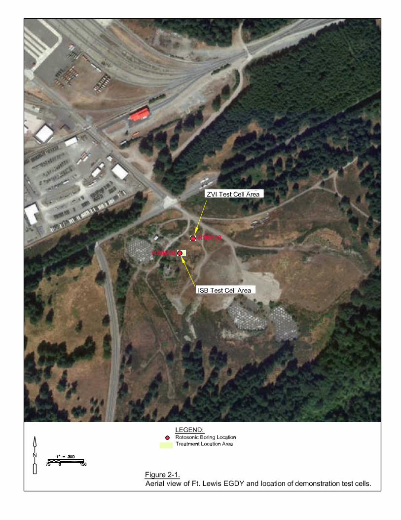

Figure 2-2. Potential reactions during ISB.
TCE
DCE
VC
Ethene
H2
H2
H2
Organic Substrate
Hydrogenolysis
TCE (or other chloroethenes)
Chloroacetylene
Acetylene
Ethene Ethane
Fe(III)
Fe(II)
Fe(III)
H2Organic acid
Organic Substrate
Reductive β elimination
bacteriabacteria
bacteriaFe(III)
Fe(II)
DCE or VC
Aerobic or Anaerobic Direct Metabolism
O2
H2O

Figure 2-3. Potential reactions with ZVI.
TCE
DCE
VC
Ethene
H2
H2
H2
Hydrogenolysis
TCE (or other chloroethenes)
Chloroacetylene
Acetylene
Ethene Ethane
Fe(0)
Fe(II)Reductive β elimination
H2O
Fe(0) emulsion material (if present)
bacteria
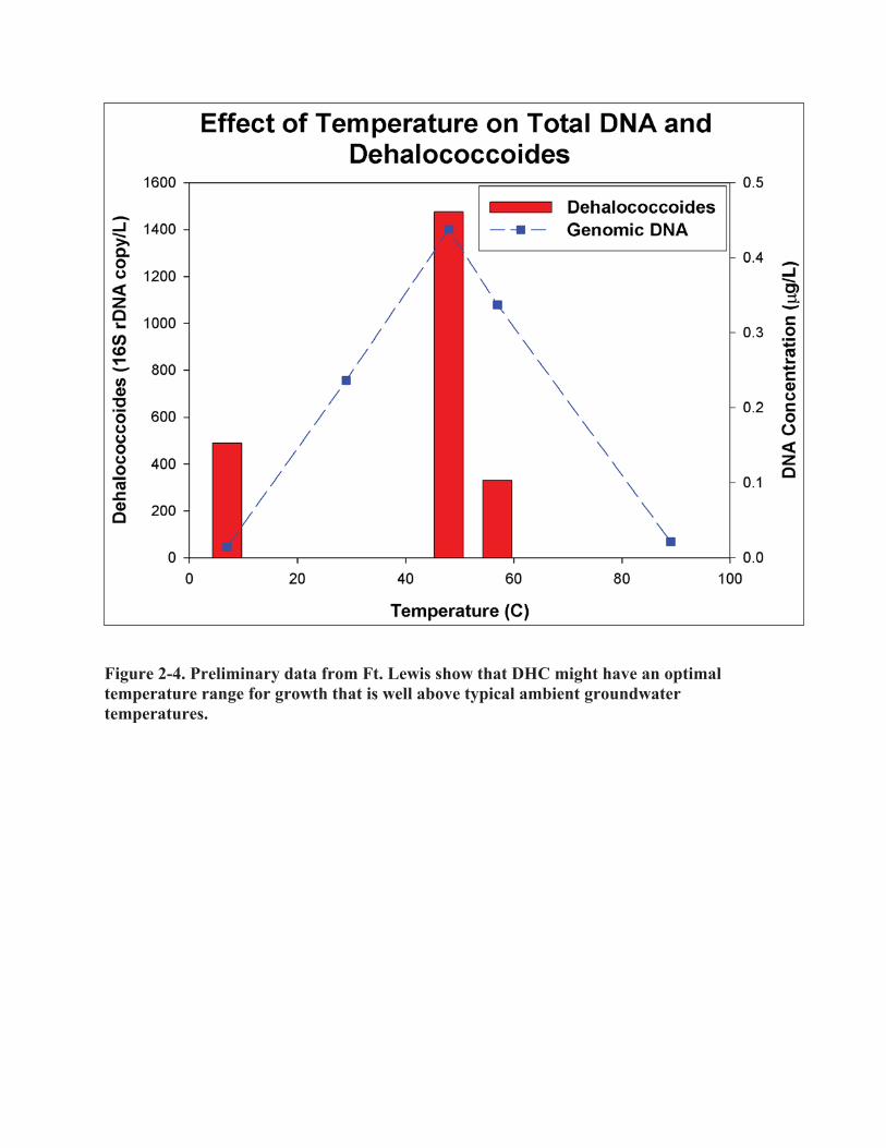
Figure 2-4. Preliminary data from Ft. Lewis show that DHC might have an optimal temperature range for growth that is well above typical ambient groundwater temperatures.

Section 2 • Technology Description
12
ESTCP ER-0719 Final Report
treatment at Fort Lewis Landfill 2, suggesting that DHC concentrations were higher at 48°C compared to ambient (10°C) (note: represents the natural response in groundwater where no other change in condition, besides a change in temperature, was effected).
In addition, Figure 2-5 illustrates the response of DHC 16S rRNA gene and functional reductase genes tceA, bvcA, and vcrA at Fort Lewis NAPL Area 3 before and during ERH heating. DHC had been enriched at this location during ESTCP project ER-0218, which evaluated bioremediation in a source area. Following the onset of heating, a two order of magnitude increase in DHC and functional genes was observed at 33°C relative to ambient temperature (approximately 12°C). At high temperatures (>70°C), however, DHC concentrations were significantly reduced and only detected near the method detection limit (MDL).
2.3 ZVI Technology Application of injectable ZVI and factors related to combination of ZVI with heating are described in detail by Truex et al. (2010 and 2011) and summarized in this section. Zero-valent iron (ZVI) has been developed and applied for in situ remediation of inorganic compounds and chlorinated solvents. Reaction mechanisms for ZVI and chlorinated solvents have been described by Arnold and Roberts (2000) and Roberts et al. (1996). Abiotic reductive elimination reactions facilitated by ZVI are beneficial for treatment of chlorinated contaminants, such as TCE), because no persistent hazardous degradation products are generated. ZVI reactions can also directly generate dichloroethene (DCE) (Arnold and Roberts 2000; Su and Puls 1999) and indirectly generate DCE (Hendrickson et al. 2002) and vinyl chloride (VC) (Maymo-Gatell et al. 1997) through facilitation of biotic reductive dechlorination. Initial kinetics of TCE dechlorination by ZVI are relatively fast and have been studied as a function of temperature (Su and Puls 1999), TCE concentration (Orth and Gillham 1996; Grant and Kueper 2004), type of iron (Miehr et al. 2004; Lin and Lo 2005; Ebert et al. 2006), and presence of multiple chlorinated solvents and other organic and inorganic species (Dries et al. 2004; Dries et al. 2005; D’Andrea et al. 2005). While initial kinetics of ZVI reactions are relatively fast, reaction kinetics can diminish over time due to corrosion and mineral precipitation, and the rate and extent of decrease in reaction rates are a function of groundwater chemistry (Farrell et al. 2000; D’Andrea et al. 2005; Kohn and Roberts 2006). Hydrogen is produced by ZVI reactions with water (Reardon et al 1995) and may stimulate biotic dechlorination of TCE with products including DCE, VC, and ethene.
A key aspect of ZVI application is successful distribution of sufficient ZVI particles in the subsurface to allow for necessary contact and reaction with the contaminant of concern (COC). Installation via trenching or physical mixing has been implemented (Wadley et al. 2005; ITRC 2005) but is not relevant for some situations. ZVI can be emplaced in an aquifer as either nano-scale or micron-scale particles. For longevity and overall cost-effectiveness, micron-scale particles are preferred, but injection of these particles using a standard groundwater well can be problematic. Their high density and size prevent the particles from being suspended in water and they cannot be injected without some form of facilitated transport. Research on improved injection strategies for iron particles has been conducted using emulsified oil (Quinn et al. 2005),

Figure 2-5. Ft. Lewis NAPL Area 3 data showing the response of DHC and functional reductase genes tceA, bvcA, and vcrA on increasing temperature during thermal heating during the ERH remedy.
H06
09/04/06 09/18/06 10/02/06 10/16/06 10/30/06
Gen
e co
pies
/L g
roun
dwat
er
1e+0
1e+1
1e+2
1e+3
1e+4
1e+5
1e+6
1e+7
1e+8
1e+9
1e+10
Tem
pera
ture
(C)
0
20
40
60
80
100
tceAbvcAvcrA16S rRNA geneTemperature

Section 2 • Technology Description
14
ESTCP ER-0719 Final Report
hydrofracturing of the aquifer (Schnell and Mack 2003), use of carrier particles (Schrick et al. 2004), and co-injection of iron with polymers (Cantrell et al. 1997a,b; Oostrom et al. 2005, 2007). Shear-thinning polymers have been demonstrated to improve transport characteristics of micron-scale ZVI and show considerable promise for emplacing ZVI within the subsurface. These polymers have been shown to promote distribution of ZVI particles in columns and meter-scale wedge-shaped flow cells (Cantrell et al. 1997a, b; Oostrom et al. 2005, 2007), but have not been field-demonstrated.
Shear-thinning fluids are non-Newtonian fluids in that their viscosity is a function of the fluid shear rate, with higher shear resulting in lower fluid viscosity. The static viscosity of the fluid may be relatively high (e.g., 100 cP). With no shear-thinning properties, injection of a 100 cP fluid into porous media would require significant pressure. However, when a shear-thinning fluid is injected into porous media, movement through the pores creates high shear conditions and the viscosity decreases significantly, enabling injection at moderate pressure (Zhong et al. 2008). Shear-thinning fluids are effective for transporting ZVI particles because the high static viscosity of the fluid results in a low settling rate for the particles compared to the settling rate in water. Thus, the ZVI particles stay suspended for a relatively long time and can be moved through the porous media. The distance that the particles can be transported is a function of how far the fluid can be moved before the particles settle and contact the sediment. Filtration of particles also limits movement, so the ZVI particles must be sufficiently small relative to the pore size to minimize filtration.
An additional benefit of using shear-thinning fluid for applications that target residual contaminant mass in soils is that the treatment volume, once emplaced, can be designed to be hydraulically isolated. During injection, the ZVI particles are carried into the targeted zone and injection pressures remain moderate due to the shear-thinning effect. Once injection ceases, however, the shear rate declines and the fluid viscosity returns to near the static value. Because the injected fluid, at low velocity, has a much higher viscosity than the groundwater (i.e., 100 cP compared to 1 cP for water), the groundwater cannot readily displace the injected solution. In an unconfined aquifer, the groundwater tends to bypass the higher viscosity injected fluid rather than displace it. Thus, the injected fluid forms a relatively isolated treatment volume within the injection zone until the shear-thinning fluid degrades or dissipates. While isolated, the desired dechlorination reactions can proceed with minimal influx of dissolved oxygen (DO) and other solutes that can passivate the ZVI. For permeable barrier applications, flow through the barrier would be slow until the shear-thinning fluid dissipates or degrades. Use of shear-thinning fluids for creating a permeable reactive barrier and the rate of shear-thinning fluid dissipation were not investigated in this effort.
In situ remediation using ZVI, similar to other in situ remedies, has potential benefits including, destruction of contaminants without generation of secondary waste streams, limited hazards to workers and the environment, relatively low capital and maintenance costs, and generally minimal disturbance of the site. For in situ remedies such as the application of injectable ZVI amendments, contaminant mass destruction only occurs in the aqueous phase. Thus, the

Section 2 • Technology Description
15 ESTCP ER-0719 Final Report
effectiveness and timeframe of these technologies, especially when applied where non-aqueous phase or significant sorbed contaminant mass is present, can be impacted by limitations in mass transfer of contaminants to the aqueous phase.
Enhanced mass transfer rate of contaminants from sorbed or DNAPL phases to the aqueous phase has been demonstrated during in situ treatment through: 1) increasing the degradation reaction rate can increase the concentration gradient between the DNAPL and water interface (Yang 2000; Cope 2001; Yang 2002; Christ 2007) and can generate more soluble, less sorbing degradation daughter products which increases the amount of contaminant mass that can be carried in the aqueous phase (Carr 2000); and 2) environmental conditions can be manipulated to enhance mass transfer (e.g. dissolution) of contaminants to the aqueous phase using cosolvents (Imhoff et al 1995), surfactants (Johnson et al 1999; Rathfeldera 2003, Singh 2007), and through dissolved organic matter partitioning (Macbeth 2008). Combining subsurface heating with in situ treatment has the potential to accelerate mass transfer further and to enhance remediation performance because higher temperatures can increase degradation reaction rates, dissolution, and volatilization.
The rate of both biologically-mediated reactions and ZVI reactions are expected to increase from temperatures typical of most groundwater systems (10-12˚C) to reach a maximum and then decline with further temperature increase. This type of temperature function is well documented for microbial processes (Atlas and Bartha 1987; Empadinhas et al 2004; Suyama et al 2002), and for reductive dechlorination reactions in particular (Kohring et al 1989, Holliger 1993, He 2003), and was observed for ZVI dechlorination processes (section 5.3). Note that the rate of some reactions, such as hydrolysis, may also continue to increase with increasing temperature.
Contaminant dissolution and volatilization generally increase with increasing temperature (Yaws et al. 2009, Sleep and Ma 1997, Horvath 1982). Typical thermal treatment applications increase temperatures to near the boiling point and mobilize DNAPL through generation of vapors which are extracted and treated. Imhoff et al, 1997 empirically and predicatively demonstrated that moderate temperature applications of hot water flushing for chlorinated solvent treatment enhance the mass transfer rate of residual DNAPL by a factor of four to five when temperatures were increased from 5 degrees Celsius (oC) to 60oC. Combining subsurface heating to moderate temperatures with in situ technologies, such as such as ZVI could negate the requirement for vapor extraction and treatment, which is a large fraction of the cost of typical thermal applications that reach boiling temperatures. For this approach to be viable, however, increases in physical mass transfer rates for both dissolution and volatilization as temperature increases must be balanced by reaction or contaminants will migrate out of the heated treatment zone without being degraded.
2.4 Advantages and Limitation of the Technology Factors significantly affecting cost and performance of this technology include:
Ability to identify the NAPL or sediment-associated contaminants and adequately deliver electron donor or ZVI. This factor is associated with site-specific properties,

Section 2 • Technology Description
16
ESTCP ER-0719 Final Report
including depth, permeability and heterogeneity of the formation, and NAPL/sediment-associated contaminant distribution. This factor can be assessed by baseline characterization using NAPL-locating techniques, including geophysics, tracer tests, groundwater sampling, and boreholes. This factor can be addressed by installing adequate numbers of electron donor and/or ZVI injection wells in the source area and/or adjusting volumes and/or concentrations of amendments used to achieve adequate contact. Wells may be screened or packers installed to target selected intervals for amendment delivery.
Ability to treat large source mass. Both ZVI and ISB would have a limited overall capacity for source treatment. Zones with high NAPL saturation would require a high dosing of ZVI or ISB substrates and long treatment times. In those cases, other treatment approaches may be more cost effective.
Presence/absence of a microbial community capable of complete conversion of TCE to ethene (ISB test cell). This factor can be assessed through baseline sampling for the presence/absence of VC and ethene; or through molecular evaluation of the microbial community, including quantitative polymerase chain reaction (qPCR) or deoxyribonucleic acid (DNA) based microarrays. These latter techniques can identify specific ribosomal DNA community profiles for comparison to those known to perform complete dechlorination. This factor may be addressed through bioaugmentation.
There are significant advantages of coupling low energy thermal treatment with either ISB or ZVI injections relative to implementing each of these technologies alone. These include:
Minimal above ground infrastructure—The coupling of in situ technologies with moderate heating negates the need for above ground treatment systems generally necessary for conventional thermal applications.
Lower safety hazards—Moderate heating also has the advantage of minimizing safety hazards associated with high temperature heating of the subsurface.
Low risks—The remediation strategies take advantage of in situ treatment where most or all of the contaminant treatment occurs in the soil or groundwater, thereby reducing risks to human health and the environment during implementation compared to ex situ technologies.
Low secondary waste generation—Most of the contaminant treatment occurs on-site, with little off-site disposal of residuals required. In addition, secondary treatment usually associated with thermal treatment (i.e., soil vapor (SV) extraction and ex-situ treatment) will not be required.
Lower cost—The cost assessment from the field demonstration showed moderate cost increases by adding heating infrastructure, in addition, the technology can be coupled to high temperature thermal applications where much of the infrastructure is already available.

Section 2 • Technology Description
17 ESTCP ER-0719 Final Report
Overall risk reduction—Demonstration data show that heating-enhanced ZVI and ISB can achieve moderate treatment endpoint conditions for groundwater and sediment contamination.
These technologies, however, face several limitations, including:
Greater uncertainty in treatment performance and life cycle costs. Uncertainties are inherent with in situ processes because conditions throughout the entire targeted region cannot be explicitly manipulated to create conditions that are optimal for the desired in situ reaction at all locations in the subsurface.
Site-specific conditions can limit application of many in situ remedial technologies, including complex lithology, low permeability media, and/or complex geochemistry.

Section 2 • Technology Description
18
ESTCP ER-0719 Final Report
This page intentionally left blank

19 ESTCP ER-0719 Final Report
SECTION 3 PERFORMANCE OBJECTIVES As previously stated, the overall objective of this demonstration was to evaluate the cost-benefit of applying low-energy ERH in combination with ISB and iron-based reduction technologies. With this in mind, detailed performance objectives were developed for each phase of the demonstration that will help meet the overall objective. Table 3-1 outlines the overall qualitative and quantitative performance objectives for the demonstration. It is important to note that interpretation of the data relies on a comparison of the reaction kinetics and evaluation of mass balance components in soils, soil gas, and groundwater (including contaminants and reductive daughter products) between Phases 2 and 3 in each individual cell. This approach avoids the difficulties in interpretation that would be introduced due to unknown differences in hydrogeologic heterogeneity and DNAPL distribution if ambient and heating tests were conducted in separate locations. That is, it allows treatment performance measurements in Phase 3 to be normalized by those made in Phase 2 in each cell. For instance, changes in treatment efficiency from Phase 2 to Phase 3 within a cell were used to quantify the effect of heating on remediation performance. The cost benefit of heating was also assessed.
Information for the cost benefit assessment includes the capital and operating cost data for the amendments, injection/hydraulic control systems, and heating system and demonstration data used to estimate the remediation timeframe and operational conditions necessary for the ambient temperature and the heated treatment. For instance, amendment quantities, electricity usage, equipment costs, and labor requirements were tracked during the test (see Section 5). The contaminant degradation rate data was measured and used to estimate treatment timeframe. This information was then used to develop a life-cycle cost estimate, including capital and operating costs and a present value assessment, so that overall remediation costs for the ambient and heated treatments can be effectively compared.

Section 3 • Performance Objectives
20
ESTCP ER-0719 Final Report
Table 3-2. Performance Objectives. Type of
Performance Objective
Primary Performance Criteria
Performance (Metric)
Qualitative
Induce dechlorination of chlorinated ethenes.
Dechlorination to desired endpoints will be achieved in each treatment cell.
Reduction in parent compounds and accumulation of abiotic and/or biotic reductive daughter products.
Biotic contaminant removal will be the primary mechanism at ambient and elevated temperature in the ISB test cell. Abiotic and biotic contaminant removal will be significant in the ZVI test cell at ambient temperature; however, abiotic mechanisms will predominate at elevated temperature.
Quantitative
Characterize nature of contamination with test cell.
Sufficient contaminant mass will be present in both test cells to meet demonstration objectives.
Define rate of dechlorination as a function of temperature.
The rate of dechlorination will be enhanced at elevated temperature in both test cells relative to ambient temperature.
Quantify test cell mass balance and loss mechanisms for chlorinated ethenes in the test cells as a function of temperature.
Contaminant mass removal will be enhanced at elevated temperature in both test cells relative to ambient temperature.
Evaluate cost-effectiveness of heating.
The overall treatment efficiency at elevated temperature will be enhanced sufficiently to offset the cost of heating in both test cells.
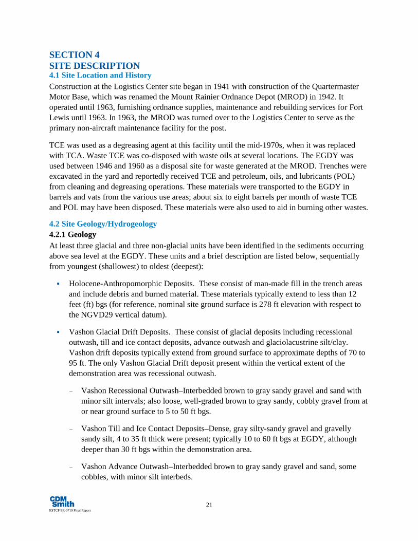
21 ESTCP ER-0719 Final Report
SECTION 4 SITE DESCRIPTION 4.1 Site Location and History Construction at the Logistics Center site began in 1941 with construction of the Quartermaster Motor Base, which was renamed the Mount Rainier Ordnance Depot (MROD) in 1942. It operated until 1963, furnishing ordnance supplies, maintenance and rebuilding services for Fort Lewis until 1963. In 1963, the MROD was turned over to the Logistics Center to serve as the primary non-aircraft maintenance facility for the post.
TCE was used as a degreasing agent at this facility until the mid-1970s, when it was replaced with TCA. Waste TCE was co-disposed with waste oils at several locations. The EGDY was used between 1946 and 1960 as a disposal site for waste generated at the MROD. Trenches were excavated in the yard and reportedly received TCE and petroleum, oils, and lubricants (POL) from cleaning and degreasing operations. These materials were transported to the EGDY in barrels and vats from the various use areas; about six to eight barrels per month of waste TCE and POL may have been disposed. These materials were also used to aid in burning other wastes.
4.2 Site Geology/Hydrogeology 4.2.1 Geology At least three glacial and three non-glacial units have been identified in the sediments occurring above sea level at the EGDY. These units and a brief description are listed below, sequentially from youngest (shallowest) to oldest (deepest):
Holocene-Anthropomorphic Deposits. These consist of man-made fill in the trench areas and include debris and burned material. These materials typically extend to less than 12 feet (ft) bgs (for reference, nominal site ground surface is 278 ft elevation with respect to the NGVD29 vertical datum).
Vashon Glacial Drift Deposits. These consist of glacial deposits including recessional outwash, till and ice contact deposits, advance outwash and glaciolacustrine silt/clay. Vashon drift deposits typically extend from ground surface to approximate depths of 70 to 95 ft. The only Vashon Glacial Drift deposit present within the vertical extent of the demonstration area was recessional outwash.
- Vashon Recessional Outwash–Interbedded brown to gray sandy gravel and sand with minor silt intervals; also loose, well-graded brown to gray sandy, cobbly gravel from at or near ground surface to 5 to 50 ft bgs.
- Vashon Till and Ice Contact Deposits–Dense, gray silty-sandy gravel and gravelly sandy silt, 4 to 35 ft thick were present; typically 10 to 60 ft bgs at EGDY, although deeper than 30 ft bgs within the demonstration area.
- Vashon Advance Outwash–Interbedded brown to gray sandy gravel and sand, some cobbles, with minor silt interbeds.

Section 4 • Site Description
22 ESTCP ER-0719 Final Report
- Glaciolacustrine Silt/Clay–Gray, laminated to massive silt and clayey silt with minor fine sand interbeds. Also very stiff to hard, dark gray clayed massive silt varying in thickness from 10 to 150 ft, typically between depths of 80 and 230 ft.
- Olympia Beds–Mottled, massive, organic-rich clayey sandy gravel or lavender silt, peat, sand and gravelly sand. May be up to 40 ft thick. May not be present in the demonstration area.
- Pre-Olympia Drift–Gray to brown, fine-to medium-grained sand with minor sandy gravel interbeds, oxidized at the top, common silt interbeds at the base, with discontinuous till. Where present this unit is typically 10 to 70 ft thick.
- Second Non-Glacial Deposits–Mottled, massive, organic rich, clayey, sandy gravel (mudflows) or lavender silt, peat, sand, and gravelly sand (fluvial overbank deposits).
- Third Glacial Drift–Interbedded, orange to dark gray sand gravel and sand with minor silt interbeds, intensely iron oxide-stained at top (recessional outwash), dense, gray, silty, sandy gravel and gravelly sandy silt (till); and interbedded, gray to brown, to dark gray sandy gravel and sand with minor silt interbeds (advance outwash).
- Third Non-Glacial Deposits–Lavender silt, peat, sand and gravelly sand.
4.2.2 Hydrogeology The primary aquifers and aquitards are listed below, sequentially from shallowest to deepest:
Vashon Aquifer or Upper Aquifer. The Vashon drift, Olympia beds, and Pre-Olympia drift comprise the Vashon unconfined aquifer. Vashon till and Olympia beds may act locally as discontinuous aquitards within the Vashon aquifer. Vashon outwash and pre-Olympia drift deposits comprise the aquifer materials within the Vashon aquifer. The Vashon aquifer varies in thickness from 100 to 130 ft and is continuous throughout the EGDY.
Intermediate Aquitard. A somewhat laterally continuous till layer may separate the Vashon aquifer locally into an upper and lower permeable unit separated by this relatively low-permeability till or glaciolacustrine silt. This till is notably absent immediately north of NAPL area 3 where low permeability units do not separate the upper and lower portions of the Vashon aquifer. The demonstration was performed in the upper Vashon aquifer, above the intermediate aquitard.
Non-Glacial Aquitard. A regional aquitard consisting of low permeability second non glacial deposits separating the Vashon aquifer from the Sea Level (lower) aquifer.
Sea Level Aquifer. Third glacial drift deposits and permeable lower deposits of the second non-glacial unit comprise the Sea Level aquifer. This unit is widely used as a source of groundwater for industrial and municipal use.
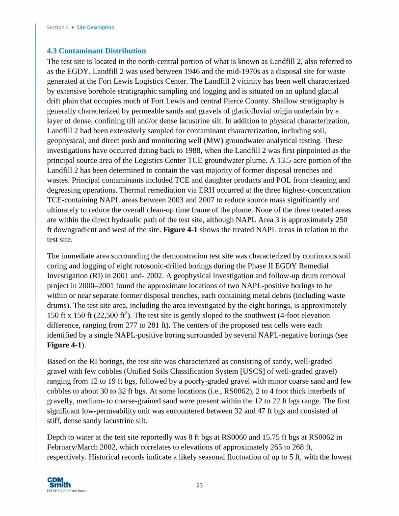
Section 4 • Site Description
23 ESTCP ER-0719 Final Report
4.3 Contaminant Distribution The test site is located in the north-central portion of what is known as Landfill 2, also referred to as the EGDY. Landfill 2 was used between 1946 and the mid-1970s as a disposal site for waste generated at the Fort Lewis Logistics Center. The Landfill 2 vicinity has been well characterized by extensive borehole stratigraphic sampling and logging and is situated on an upland glacial drift plain that occupies much of Fort Lewis and central Pierce County. Shallow stratigraphy is generally characterized by permeable sands and gravels of glaciofluvial origin underlain by a layer of dense, confining till and/or dense lacustrine silt. In addition to physical characterization, Landfill 2 had been extensively sampled for contaminant characterization, including soil, geophysical, and direct push and monitoring well (MW) groundwater analytical testing. These investigations have occurred dating back to 1988, when the Landfill 2 was first pinpointed as the principal source area of the Logistics Center TCE groundwater plume. A 13.5-acre portion of the Landfill 2 has been determined to contain the vast majority of former disposal trenches and wastes. Principal contaminants included TCE and daughter products and POL from cleaning and degreasing operations. Thermal remediation via ERH occurred at the three highest-concentration TCE-containing NAPL areas between 2003 and 2007 to reduce source mass significantly and ultimately to reduce the overall clean-up time frame of the plume. None of the three treated areas are within the direct hydraulic path of the test site, although NAPL Area 3 is approximately 250 ft downgradient and west of the site. Figure 4-1 shows the treated NAPL areas in relation to the test site.
The immediate area surrounding the demonstration test site was characterized by continuous soil coring and logging of eight rotosonic-drilled borings during the Phase II EGDY Remedial Investigation (RI) in 2001 and- 2002. A geophysical investigation and follow-up drum removal project in 2000–2001 found the approximate locations of two NAPL-positive borings to be within or near separate former disposal trenches, each containing metal debris (including waste drums). The test site area, including the area investigated by the eight borings, is approximately 150 ft x 150 ft (22,500 ft2). The test site is gently sloped to the southwest (4-foot elevation difference, ranging from 277 to 281 ft). The centers of the proposed test cells were each identified by a single NAPL-positive boring surrounded by several NAPL-negative borings (see Figure 4-1).
Based on the RI borings, the test site was characterized as consisting of sandy, well-graded gravel with few cobbles (Unified Soils Classification System [USCS] of well-graded gravel) ranging from 12 to 19 ft bgs, followed by a poorly-graded gravel with minor coarse sand and few cobbles to about 30 to 32 ft bgs. At some locations (i.e., RS0062), 2 to 4 foot thick interbeds of gravelly, medium- to coarse-grained sand were present within the 12 to 22 ft bgs range. The first significant low-permeability unit was encountered between 32 and 47 ft bgs and consisted of stiff, dense sandy lacustrine silt.
Depth to water at the test site reportedly was 8 ft bgs at RS0060 and 15.75 ft bgs at RS0062 in February/March 2002, which correlates to elevations of approximately 265 to 268 ft, respectively. Historical records indicate a likely seasonal fluctuation of up to 5 ft, with the lowest
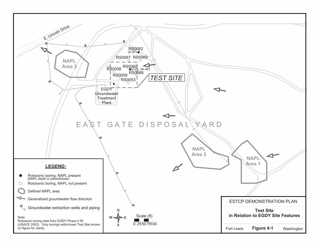
RS0060
RS0069
RS0068
RS0053
RS0058RS0059
WashingtonFigure 4-1Fort Lewis
Test Sitein Relation to EGDY Site Features
ESTCP DEMONSTRATION PLAN
E. Lincoln Drive
0 255075100
Scale (ft)
NAPLArea 3
NAPLArea 2
NAPLArea 1
E A S T G A T E D I S P O S A L Y A R D
Note:Rotosonic boring data from EGDY Phase II RI (USACE 2002). Only borings within/near Test Site shown on figure for clarity.
(NAPL depth in parentheses)Rotosonic boring, NAPL present
Rotosonic boring, NAPL not present
Defined NAPL area
Generalized groundwater flow direction
Groundwater extraction wells and piping
LEGEND:
(5-20')
(2-25, 34-36')
EGDYGroundwater
TreatmentPlant
TEST SITE
RS0067
RS0062

Section 4 • Site Description
25 ESTCP ER-0719 Final Report
groundwater levels in October and the highest levels in April. The horizontal hydraulic gradient is approximately 0.004 ft/ft in a westerly to southwesterly direction.
NAPL was observed within one of the NAPL-positive borings from approximately 5 to 20 ft bgs (designated RS0062) consisting predominantly of TCE (up to 25 mg/kg) and cis-DCE (up to 16.4 mg/kg). TCE was the predominant constituent (up to 2,460 mg/kg) within the second NAPL positive boring (RS0060), which contained NAPL from 2 to 25 ft bgs and 34 to 36 ft bgs. No cis-DCE was detected in samples from this boring. See Figure 4-2 for a summary of existing TCE and DCE analytical results. NAPL consisting primarily of TCE from approximately 10 to 18 ft bgs was interpreted at membrane interface probe boring SM0030 conducted as part of the RI, as shown on Figure 4-3. All of the NAPL contamination was observed to be within permeable gravels and sands. Figure 4-3 illustrates results of membrane interface probe SM0030 located at the edge of the EGDY groundwater treatment plant.

276
278
27627
6
278
280
DP-1
DP-15
DP-21
DP-22
DP-24
DP-32
DP-38
RS0060
RS0069
RS0068
RS0053
RS0058
RS0059
WashingtonFigure 4-2Fort Lewis
Test SiteExisting Sample Locations and Results
ESTCP DEMONSTRATION PLAN
0 25 50 75 100
Scale (ft)
Notes:1. Rotosonic boring data from EGDY 2002 Phase II RI. 2. Drive-point groundwater locations from 1999 Phase I RI.
(NAPL depth in parentheses)Rotosonic boring, NAPL present
Rotosonic boring, NAPL not present
MIP boring, NAPL present
Drive-point groundwater location
Generalized groundwater flow direction
Removed drum
Magnetic anomaly
Ground surface contour (ft)
LEGEND:
(5-20')
(2-25, 34-36')
EGDYGROUNDWATER
TREATMENT PLANT
RS0067
RS0062 RS0062 (soil, ug/kg) TCE cis-DCE7-7.5 ft: 25,000 2,38013-14 ft: 10,600 16,40023.5-24 ft: 2,030 ND36-37 ft: 327J ND
RS0060 (soil, ug/kg) TCE cis-DCE6-7 ft: 2,460,000 ND17-18 ft: 206,000 ND26-27 ft: 2,790 ND40-41 ft: ND ND47-48 ft: ND ND57-58 ft: ND ND
DP-22 (groundwater, ug/l) TCE cis-DCE10 ft: 42 1.316 ft: 51 3.624 ft: 1,800 5732 ft: 61 69
RS0069 (soil, ug/kg) TCE cis-DCE16-17 ft: ND ND30-31 ft: 3,100 ND
RS0067 (soil, ug/kg) TCE cis-DCE9-9.5 ft: 2,100 ND26-27 ft: 546 ND
RS0058 (soil, ug/kg) TCE cis-DCE7-8 ft: 2,610 59025-26 ft: 2,310 ND35-36 ft: 504 ND36-37 ft: 682 ND
RS0059 (soil, ug/kg) TCE cis-DCE10-11 ft: 3,620 26710-11 ft Dup: 4,600 40130-31 ft: 532 ND
RS0068 (soil, ug/kg) TCE cis-DCE6-7 ft: ND ND25-26 ft: ND ND
DP-32 (groundwater, ug/l) TCE cis-DCE10 ft: 220 5.319 ft: 960 <2524 ft: 2,200 8628 ft: 840 <125
RS0053 (soil, ug/kg) TCE cis-DCE8-9 ft: ND 10519-20 ft: 195 ND30.5-31 ft: 2,010 22653-54 ft: ND ND
T E S T
S I T E
Membrane Interface Probe (MIP) SM0030(NAPL inferred 10-18')

Figure 4-3. Results of Membrane Interface Probe data collected during the RI at SM0030 located at the corner of EGDY Treatment Plant.
8

Section 4 • Site Description
28 ESTCP ER-0719 Final Report
This page intentionally left blank

29 ESTCP ER-0719 Final Report
SECTION 5 TEST DESIGN 5.1 Conceptual Experimental Design This demonstration was designed to evaluate the benefits of low-energy ERH combined with ISB and iron-based reduction technologies for treatment of chlorinated solvent residual source areas. The demonstration included use of two test cells to evaluate each combination of technologies. The demonstration was executed in three phases, including:
Phase 1: Initial characterization and verification of the suitability of each test cell to meet project objectives, which provided information for a “go/no-go” decision on test cell placement. Once the test site was selected, each treatment system was installed with implementation of hydraulic characterization and baseline sampling.
Phase 2: Field demonstration of ISB and ZVI without heating. This phase of the demonstration established the reaction kinetics and mass balance factors at ambient temperature.
Phase 3: Field demonstration of ISB and ZVI with low-energy ERH. This phase of the demonstration established reaction kinetics and mass balance factors at elevated temperatures of approximately 35°C for the ISB cell and 55°C for the ZVI cell. Results were compared to Phase 2 to determine if objectives were met.
Phase 1 of the demonstration included pre-design characterization to determine the suitability of the test cells for the demonstration (i.e., confirm presence of sufficient residual DNAPL mass within the test cell); test cell installation, baseline contaminant characterization via groundwater sampling, soil gas sampling, and soil boring and sampling; and hydraulic tracer testing within the ISB test cell (note that for the ZVI test cell, tracer was injected along with the ZVI amendment and so is discussed as part of Phase 2 for that test cell).
Phase 2 of the demonstration evaluated performance of the ISB and ZVI in situ technologies at ambient groundwater temperatures. This phase included amendment injection, groundwater, soil gas, and soil boring and sampling as a baseline for comparison to the heated condition (Phase 3).
Phase 2 activities for the ISB test cell included establishing efficient anaerobic reductive dechlorination (ARD) at ambient temperature through injection of electron donors, emulsified oil (EOS®) and then whey powder. Relatively low substrate concentrations were used in the test to minimize the substrate impact on dissolution so that increases in dissolution could be primarily attributed to temperature and ARD. The desired transformation reactions, which convert TCE to DCE, VC, and ultimately to ethene are illustrated in Figure 2-2. In addition, some sediment iron reduction and subsequent TCE dechlorination may occur once anaerobic conditions are established, dependent on the presence, extent, and availability of reducible iron (Szecsody et al. 2004). During the ISB study, products of each reaction shown on Figure 2-2 were measured in soils, groundwater, and soil gas, as appropriate, to determine the relative rates of these reactions at ambient test temperatures. The extent and rate of ARD and contaminant mass removal will be

Section 5 • Test Design
30
ESTCP ER-0719 Final Report
established under the ambient temperatures. In addition, a mass balance approach was used to evaluate mass reduction rates and extents based on a mass-discharge approach.
Phase 2 activities for the ZVI test cell included first establishing in situ destruction of TCE using injectable micron-scale ZVI (see Truex et al. 2010 for details). The ZVI injection concentration was established based on laboratory treatability studies. The desired primary transformation reaction converts TCE to ethene and ethane via beta-elimination, and is illustrated in Figure 2-3. In addition to abiotic reactions, some biological transformation was expected due to hydrogen production (also illustrated in Figure 2-3), although potentially some reductive dechlorination may occur through direct interaction with the ZVI. During the ZVI study, products of each reaction were measured in soils, groundwater and soil gas, as appropriate, to determine the relative rates of these reactions at ambient temperatures. In addition, a mass balance approach was used to evaluate mass reduction rates and extents based on a mass-discharge approach (see Truex et al. 2011 for details).
Phase 3 of the demonstration evaluated the effect of low-temperature heating of the test cells to 30 to 40°C for the ISB cell and 40-50°C for the ZVI test cell. Again, groundwater, soil gas, and soil boring and sampling data were collected. In this way, the demonstration allowed for the measurement of the relative impact of heating on the overall rate and extent of TCE dechlorination under the heated condition (Phase 3) compared to the ambient condition (Phase 2) (see Truex et al. 2011 for details).
5.2 Phase 1: Baseline Characterization One of the most significant technical uncertainties of this demonstration was whether the quantity of residual contaminant mass within the test cells was sufficient to meet project objectives. A key objective of the project is to evaluate the relative increase in contaminant removal rates under heated conditions relative to the ambient condition. Therefore, sufficient residual contaminant mass in soil was required to observe enhanced mass transfer to the aqueous phase during Phases 2 and 3 of the demonstration. The selection of the planned test cells was based on two soil cores collected during the RI (2001–2002) that were positive for NAPL, suggesting favorable localized conditions for the demonstration (Figure 4-2). However, both of the NAPL-containing soil cores were surrounded by additional soil cores containing no NAPL (see Figure 4-2). Therefore, the pre-design characterization effort was undertaken to further characterize the area within and around the planned test cells. Table 5-1 illustrates the characterization activity and the objectives of the activity.
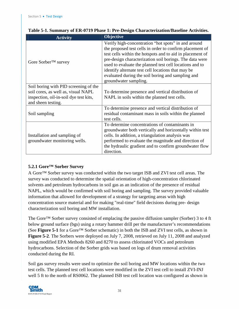
Section 5 • Test Design
31 ESTCP ER-0719 Final Report
Table 5-1. Summary of ER-0719 Phase 1: Pre-Design Characterization/Baseline Activities. Activity Objective
Gore Sorber™ survey
Verify high-concentration “hot spots” in and around the proposed test cells in order to confirm placement of test cells within the hotspots and to aid in placement of pre-design characterization soil borings. The data were used to evaluate the planned test cell locations and to identify alternate test cell locations that may be evaluated during the soil boring and sampling and groundwater sampling.
Soil boring with PID screening of the soil cores, as well as, visual NAPL inspection, oil-in-soil dye test kits, and sheen testing.
To determine presence and vertical distribution of NAPL in soils within the planned test cells.
Soil sampling To determine presence and vertical distribution of residual contaminant mass in soils within the planned test cells.
Installation and sampling of groundwater monitoring wells.
To determine concentrations of contaminants in groundwater both vertically and horizontally within test cells. In addition, a triangulation analysis was performed to evaluate the magnitude and direction of the hydraulic gradient and to confirm groundwater flow direction.
5.2.1 Gore™ Sorber Survey A Gore™ Sorber survey was conducted within the two target ISB and ZVI test cell areas. The survey was conducted to determine the spatial orientation of high-concentration chlorinated solvents and petroleum hydrocarbons in soil gas as an indication of the presence of residual NAPL, which would be confirmed with soil boring and sampling. The survey provided valuable information that allowed for development of a strategy for targeting areas with high concentration source material and for making "real-time" field decisions during pre- design characterization soil boring and MW installation.
The Gore™ Sorber survey consisted of emplacing the passive diffusion sampler (Sorber) 3 to 4 ft below ground surface (bgs) using a rotary hammer drill per the manufacturer’s recommendations (See Figure 5-1 for a Gore™ Sorber schematic) in both the ISB and ZVI test cells, as shown in Figure 5-2. The Sorbers were deployed on July 7, 2008, retrieved on July 11, 2008 and analyzed using modified EPA Methods 8260 and 8270 to assess chlorinated VOCs and petroleum hydrocarbons. Selection of the Sorber grids was based on logs of drum removal activities conducted during the RI.
Soil gas survey results were used to optimize the soil boring and MW locations within the two test cells. The planned test cell locations were modified in the ZVI test cell to install ZVI-INJ well 5 ft to the north of RS0062. The planned ISB test cell location was configured as shown in

Figure 5-1. Schematic of emplaced Gore™ Sorber.
99
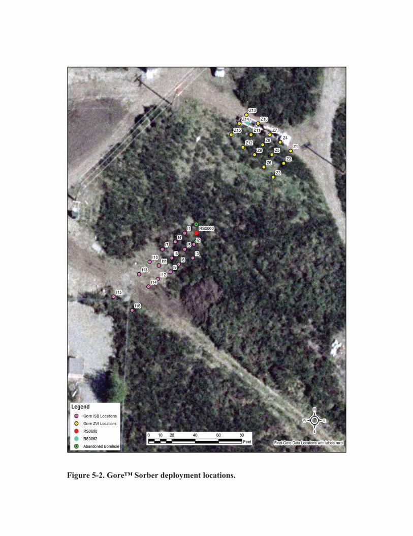
Figure 5-2. Gore™ Sorber deployment locations.

Section 5 • Test Design
34
ESTCP ER-0719 Final Report
the Demonstration Plan with ISB- MW2 corresponding to Sorber location I1 and ISB-MW1 and ISB-MW3 to the north and south of RS0060 (Figure 5-3). An alternate location was identified near Gore™ Sorber locations I15 and I16 if the soil boring and sampling indicated that one or the other test cells was not suitable. A strategy for soil boring, screening and decision criteria for MW installation was developed. The decision strategy included the following steps:
1. Soil boreholes were advanced and soil cores were collected along the entire vertical interval.
2. Photoionization detector (PID) measurements were collected along the core at approximately 2-ft intervals. Previous investigation at the site indicated that relatively high PID readings (>200 parts per million (ppm)) and visual observation of NAPL corresponded to high (>10,000 microgram per kilogram (µg/kg)) concentrations of VOCs in soils.
3. Sheen and dye testing was used to determine the presence of NAPL.
4. If PID readings indicated high concentrations of volatiles and/or if the sheen and dye testing indicated NAPL was present, three soil samples were collected from the soil intervals with the highest detected concentrations, and the groundwater well was installed within the borehole.
5. If PID readings and sheen and dye testing did not indicate the presence of contaminants, the borehole was abandoned, and the technical team convened in real time to discuss re-configuration and placement of additional boreholes.
The ability to evaluate field data and make decisions in real time about well placement was intended to maximize drilling mobilization efficiency and increase the probability of well placement in high contaminant concentration areas suitable for meeting demonstration objectives.
5.2.2 Soil Characterization and Installation of ISB Test Cell Wells Following the Gore™ Sorber survey, pre-design characterization subsurface drilling, soil sampling, and well installation was conducted. Pre-design characterization work included drilling and lithologic logging of soil borings at three locations identified as ISB-MW1, ISB-MW2, and ISB-MW3 (boring logs provided in Appendix B). These borings were originally
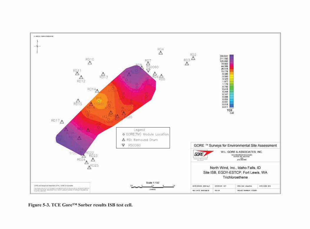
�
Figure 5-3. TCE Gore™ Sorber results ISB test cell.
101

Section 5 • Test Design
36
ESTCP ER-0719 Final Report
positioned such that the planned centerline well ISB-MW2 would be at high soil gas sample location I1, and ISB-MW1 and ISB-MW3 would be north and south of RS0060. Original locations for ISB-MW1 and ISB-MW3 were abandoned because field screening results indicated that no NAPL contaminant mass was present (Appendix B). Alternate locations that were bored, screened and completed as MWs included a location that corresponded directly with RS0060 and one that corresponded to the area between Gore™ Sorber locations I4 and I5 that indicated relatively high contaminant mass levels. Field screening results indicated both locations contained sufficiently high levels of contamination for completion as ISB-MW1 and ISB-MW3 (see Figure 5-5 for location of actual well placements).
Analytical soil samples were collected at the three depths from each soil core collected for a boring that was completed as a MW. Sample points were selected based on areas that demonstrated the highest potential for contamination based on elevated PID readings, visual NAPL evidence, dye testing and sheen testing results. Soil sample depths at ISB-MW1 occurred at 17.5, 19, and 27.5 ft bgs (Table 5-2). At ISB-MW2, sample depths were 9, 14, and 19 ft bgs; at ISB-MW3, depths were 9, 14.5, and 16 ft bgs.
Table 5-2. Summary of Baseline Analytical Results from Field Screening and Soil Sampling.
Cell Borehole Location
Analytical Sample Point (ft
bgs)
Analytical Result TCE
(µg/kg)
Analytical Result cis-1,2-DCE (µg/kg)
Maximum PID
Measurement (ppm)
Interpreted NAPL Depth
Interval
ISB
ISB-MW1
17.5 76,000 11 715 16.5-20 ft bgs 19 10,000 5.6 98
27.5 4,900 28 44
ISB-MW2
9 5,100 11 63 14.0-20 ft bgs 14 130,000 91 1,555
19 65,000 30 9,300
ISB-MW3
9 17,000 8 197 None 14.5 8,500 7.9 142
16 4,000 16 2,662
ZV
I
ZVI-INJ1 8.8 220,000 180 629
5-13 ft bgs 10.5 11,000 110 15 15.3 6,800 48 4
ZVI-MW1
11 2500 38 10.6 None 16 470 33 0.7
20.5 250 16 0.7
ZVI-MW2
12 1600 100 32.9 None 16.5 1400 34 1.4
20 1900 110 9.8 Note: Area shaded in grey indicates soil samples that met the “Go” decision criteria of 10,000 µg/kg. The grey areas that also have bold lettering indicate samples collected within the saturated interval and gray areas without bold lettering indicate samples collected within the vadose zone.

�
Figure 5-4. TCE Gore™ Sorber results ZVI test cell.
102

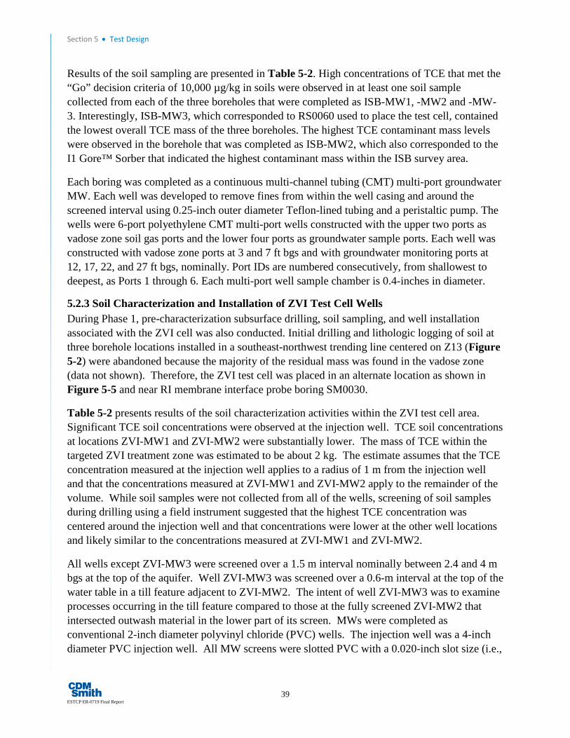
Section 5 • Test Design
39 ESTCP ER-0719 Final Report
Results of the soil sampling are presented in Table 5-2. High concentrations of TCE that met the “Go” decision criteria of 10,000 µg/kg in soils were observed in at least one soil sample collected from each of the three boreholes that were completed as ISB-MW1, -MW2 and -MW-3. Interestingly, ISB-MW3, which corresponded to RS0060 used to place the test cell, contained the lowest overall TCE mass of the three boreholes. The highest TCE contaminant mass levels were observed in the borehole that was completed as ISB-MW2, which also corresponded to the I1 Gore™ Sorber that indicated the highest contaminant mass within the ISB survey area.
Each boring was completed as a continuous multi-channel tubing (CMT) multi-port groundwater MW. Each well was developed to remove fines from within the well casing and around the screened interval using 0.25-inch outer diameter Teflon-lined tubing and a peristaltic pump. The wells were 6-port polyethylene CMT multi-port wells constructed with the upper two ports as vadose zone soil gas ports and the lower four ports as groundwater sample ports. Each well was constructed with vadose zone ports at 3 and 7 ft bgs and with groundwater monitoring ports at 12, 17, 22, and 27 ft bgs, nominally. Port IDs are numbered consecutively, from shallowest to deepest, as Ports 1 through 6. Each multi-port well sample chamber is 0.4-inches in diameter.
5.2.3 Soil Characterization and Installation of ZVI Test Cell Wells During Phase 1, pre-characterization subsurface drilling, soil sampling, and well installation associated with the ZVI cell was also conducted. Initial drilling and lithologic logging of soil at three borehole locations installed in a southeast-northwest trending line centered on Z13 (Figure 5-2) were abandoned because the majority of the residual mass was found in the vadose zone (data not shown). Therefore, the ZVI test cell was placed in an alternate location as shown in Figure 5-5 and near RI membrane interface probe boring SM0030.
Table 5-2 presents results of the soil characterization activities within the ZVI test cell area. Significant TCE soil concentrations were observed at the injection well. TCE soil concentrations at locations ZVI-MW1 and ZVI-MW2 were substantially lower. The mass of TCE within the targeted ZVI treatment zone was estimated to be about 2 kg. The estimate assumes that the TCE concentration measured at the injection well applies to a radius of 1 m from the injection well and that the concentrations measured at ZVI-MW1 and ZVI-MW2 apply to the remainder of the volume. While soil samples were not collected from all of the wells, screening of soil samples during drilling using a field instrument suggested that the highest TCE concentration was centered around the injection well and that concentrations were lower at the other well locations and likely similar to the concentrations measured at ZVI-MW1 and ZVI-MW2.
All wells except ZVI-MW3 were screened over a 1.5 m interval nominally between 2.4 and 4 m bgs at the top of the aquifer. Well ZVI-MW3 was screened over a 0.6-m interval at the top of the water table in a till feature adjacent to ZVI-MW2. The intent of well ZVI-MW3 was to examine processes occurring in the till feature compared to those at the fully screened ZVI-MW2 that intersected outwash material in the lower part of its screen. MWs were completed as conventional 2-inch diameter polyvinyl chloride (PVC) wells. The injection well was a 4-inch diameter PVC injection well. All MW screens were slotted PVC with a 0.020-inch slot size (i.e.,
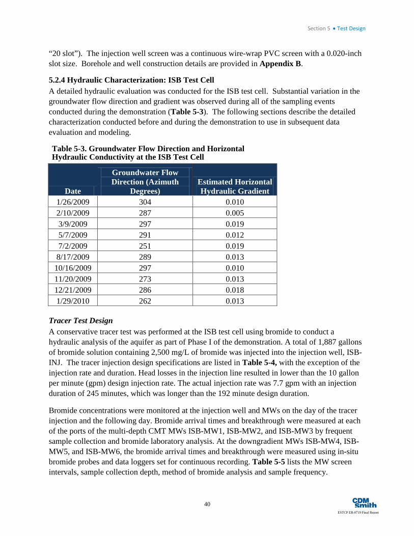
Section 5 • Test Design
40
ESTCP ER-0719 Final Report
“20 slot”). The injection well screen was a continuous wire-wrap PVC screen with a 0.020-inch slot size. Borehole and well construction details are provided in Appendix B.
5.2.4 Hydraulic Characterization: ISB Test Cell A detailed hydraulic evaluation was conducted for the ISB test cell. Substantial variation in the groundwater flow direction and gradient was observed during all of the sampling events conducted during the demonstration (Table 5-3). The following sections describe the detailed characterization conducted before and during the demonstration to use in subsequent data evaluation and modeling.
Table 5-3. Groundwater Flow Direction and Horizontal Hydraulic Conductivity at the ISB Test Cell
Date
Groundwater Flow Direction (Azimuth
Degrees) Estimated Horizontal Hydraulic Gradient
1/26/2009 304 0.010 2/10/2009 287 0.005 3/9/2009 297 0.019 5/7/2009 291 0.012 7/2/2009 251 0.019 8/17/2009 289 0.013 10/16/2009 297 0.010 11/20/2009 273 0.013 12/21/2009 286 0.018 1/29/2010 262 0.013
Tracer Test Design A conservative tracer test was performed at the ISB test cell using bromide to conduct a hydraulic analysis of the aquifer as part of Phase I of the demonstration. A total of 1,887 gallons of bromide solution containing 2,500 mg/L of bromide was injected into the injection well, ISB-INJ. The tracer injection design specifications are listed in Table 5-4, with the exception of the injection rate and duration. Head losses in the injection line resulted in lower than the 10 gallon per minute (gpm) design injection rate. The actual injection rate was 7.7 gpm with an injection duration of 245 minutes, which was longer than the 192 minute design duration.
Bromide concentrations were monitored at the injection well and MWs on the day of the tracer injection and the following day. Bromide arrival times and breakthrough were measured at each of the ports of the multi-depth CMT MWs ISB-MW1, ISB-MW2, and ISB-MW3 by frequent sample collection and bromide laboratory analysis. At the downgradient MWs ISB-MW4, ISB-MW5, and ISB-MW6, the bromide arrival times and breakthrough were measured using in-situ bromide probes and data loggers set for continuous recording. Table 5-5 lists the MW screen intervals, sample collection depth, method of bromide analysis and sample frequency.
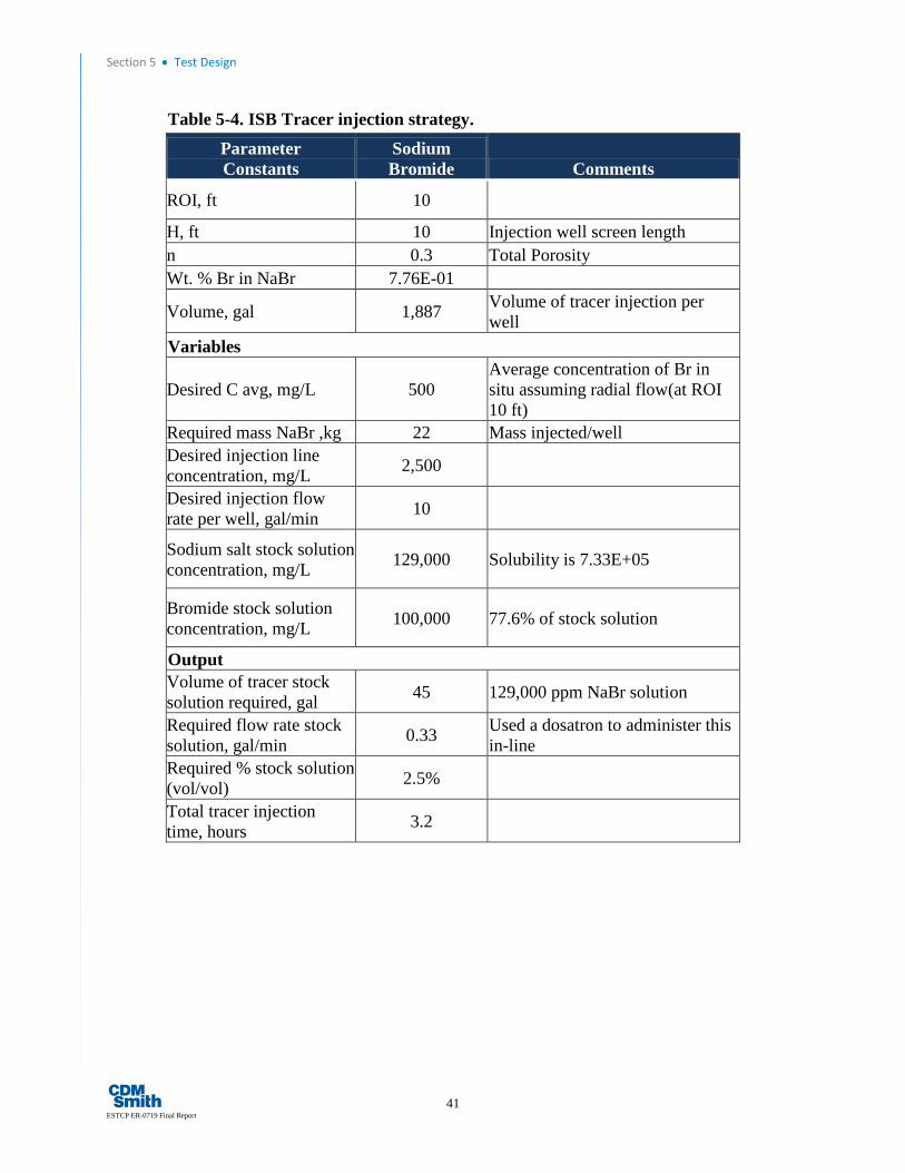
Section 5 • Test Design
41 ESTCP ER-0719 Final Report
Table 5-4. ISB Tracer injection strategy. Parameter Constants
Sodium Bromide Comments
ROI, ft 10
H, ft 10 Injection well screen length n 0.3 Total Porosity Wt. % Br in NaBr 7.76E-01
Volume, gal 1,887 Volume of tracer injection per well
Variables
Desired C avg, mg/L 500 Average concentration of Br in situ assuming radial flow(at ROI 10 ft)
Required mass NaBr ,kg 22 Mass injected/well Desired injection line concentration, mg/L 2,500
Desired injection flow rate per well, gal/min 10
Sodium salt stock solution concentration, mg/L 129,000 Solubility is 7.33E+05
Bromide stock solution concentration, mg/L 100,000 77.6% of stock solution
Output Volume of tracer stock solution required, gal 45 129,000 ppm NaBr solution
Required flow rate stock solution, gal/min 0.33 Used a dosatron to administer this
in-line Required % stock solution (vol/vol) 2.5%
Total tracer injection time, hours 3.2
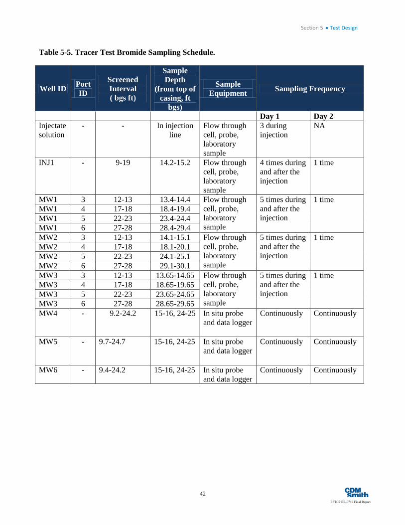
Section 5 • Test Design
42
ESTCP ER-0719 Final Report
Table 5-5. Tracer Test Bromide Sampling Schedule.
Well ID Port ID
Screened Interval ( bgs ft)
Sample Depth
(from top of casing, ft
bgs)
Sample Equipment Sampling Frequency
Day 1 Day 2 Injectate solution
- - In injection line
Flow through cell, probe, laboratory sample
3 during injection
NA
INJ1 - 9-19 14.2-15.2 Flow through cell, probe, laboratory sample
4 times during and after the injection
1 time
MW1 3 12-13 13.4-14.4 Flow through cell, probe, laboratory sample
5 times during and after the injection
1 time MW1 4 17-18 18.4-19.4 MW1 5 22-23 23.4-24.4 MW1 6 27-28 28.4-29.4 MW2 3 12-13 14.1-15.1 Flow through
cell, probe, laboratory sample
5 times during and after the injection
1 time MW2 4 17-18 18.1-20.1 MW2 5 22-23 24.1-25.1 MW2 6 27-28 29.1-30.1 MW3 3 12-13 13.65-14.65 Flow through
cell, probe, laboratory sample
5 times during and after the injection
1 time MW3 4 17-18 18.65-19.65 MW3 5 22-23 23.65-24.65 MW3 6 27-28 28.65-29.65 MW4 - 9.2-24.2 15-16, 24-25 In situ probe
and data logger Continuously Continuously
MW5 - 9.7-24.7 15-16, 24-25 In situ probe and data logger
Continuously Continuously
MW6 - 9.4-24.2 15-16, 24-25 In situ probe and data logger
Continuously Continuously

Section 5 • Test Design
43 ESTCP ER-0719 Final Report
Hydraulic Testing Results Bromide tracer arrival times were used to determine the groundwater seepage velocity during the tracer test. These results were used along with hydraulic gradient information to calculate the groundwater seepage velocity during ambient (i.e., non-injection) conditions and to estimate the hydraulic conductivity at discrete depths within the ISB test cell. The following sections describe the calculation approach and results.
Hydraulic Gradient To evaluate the horizontal hydraulic gradient during ambient conditions and during an injection event, groundwater elevation measurements were collected during the Phase 3 whey injection event that occurred on January 29, 2010. This injection took place over a 247-minute period at an average injection rate of 6.1 gpm. ISB-INJ1 was utilized as the injection well. The groundwater elevation at each of the ISB test cell MWs was measured immediately prior to and 2.9 hours after the start of the injection. The EGDY pump and treat system was operating continuously throughout the injection period.
Table 5-6 lists the groundwater elevation monitoring results, including the ambient groundwater flow direction and hydraulic gradient, the average hydraulic gradient during the injection, amount of groundwater mounding at each monitoring point, and the distance between the injection well and each monitoring point. The results indicate that the ambient groundwater flow direction and hydraulic gradient was 262° at 0.013 foot/foot and that a radial flow pattern developed as a result of the injection. Observed groundwater mounding ranged from a maximum of +0.56 ft at the MW located 7 ft away from the injection well to a minimum of +0.10 ft at the MW located 37 ft away.
Groundwater Velocity Figures 5-6, 5-7, and 5-8 show the breakthrough curves for the ISB test cell MWs (ISB-MW1, ISB-MW2, and ISB-MW3). The breakthrough curves for the downgradient MWs (ISB-MW4, ISB-MW5, and ISB-MW6) are shown in Figure 5-9. The peak of each curve represents the maximum bromide concentration or peak breakthrough. Because the tracer injection occurred as a 245-minute injection and was not instantaneous, the midpoint of the injection period, time (t) = 122.5 minutes, was selected as the start travel time (t0) for the purpose of groundwater velocity calculation. The advective travel time is the time from t0 until peak breakthrough at a particular monitoring point. The groundwater seepage velocity is derived by dividing the distance between the injection well and the MW by the advective travel time.
The advective travel times and corresponding groundwater seepage velocity for each monitoring point within the ISB test cell are listed in Table 5-7. The seepage velocities ranged from 64 to 252 ft/day within the ISB test cell during the tracer test.
The seepage velocities observed during the groundwater tracer test are much higher than ambient due to groundwater mounding centered on the injection well and the resulting increased horizontal hydraulic gradient. In order to estimate a seepage velocity under ambient conditions,

Table 5-6. Groundwater elevations during and after ISB tracer test.
East Gate Disposal Yard ISB Test CellFort Lewis, Washington
Monitoring Point ID
Distance Between Injection Well and Monitoring Point (ft)
Groundwater Elevation (ft)
Groundwater Flow Direction
Hydraulic Gradient1
(ft/ft)Groundwater Elevation (ft)
Groundwater Flow Direction
Hydraulic Gradient1
(ft/ft)
Amount of Groundwater
Mounding(ft)
ISB-INJ 0 270.31 272.35 2.04ISB-MW1-3 21 270.09 270.17 0.08ISB-MW2-3 15 270.01 270.29 0.28ISB-MW3-3 7 270.16 270.72 0.56ISB-MW4 37 269.82 269.92 0.10ISB-MW5 37 269.85 269.96 0.11ISB-MW6 36 270.12 270.17 0.05Notes:
The EGDY groundwater extraction system was operating continuously prior to and during the injection event.1 The hydraulic gradient listed is the average gradient between the ISB-MW1, ISB-MW2, ISB-MW3 well clusters and the downgradient ISB-MW4, ISB-MW5, and ISB-MW6 monitoring wells.
Radial262 0.013 0.022
Ambient Conditions During Injection - 2.9 Hours After Start
174

Table 5-7. Hydraulic parameters calculated based on the tracer test and used for calculations.
Landfill 2, Fort Lewis, Washington: ISB Test Cell
Monitoring Point
Distance from
Injection Point (ft)
Depth of
Screen (ft bgs)
Tracer Travel Time1
(minutes)
Groundwater Velocity
During Tracer Test (ft/d)
Estimated Ambient
Groundwater Velocity (ft/d)
Estimated Horizontal Hydraulic Gradient During
Tracer Test2
Estimated Effective Porosity3
Hydraulic Conductivity3
(ft/d)INJ 0 5 - 19 -- -- -- -- -- --MW1-3 21 12 440 67 31 0.028 0.18 455MW1-4 21 17 310 95 36 0.034 0.18 532MW1-5 21 22 430 69 32 0.028 0.18 466MW1-6 21 27 460 64 31 0.027 0.18 452MW2-3 15 12 240 87 28 0.040 0.18 413MW2-4 15 17 250 84 27 0.040 0.18 397MW2-5 15 22 150 139 45 0.040 0.18 661MW2-6 15 27 NA NA NA NA NA NAMW3-3 7 12 50 202 66 0.040 0.18 9585
MW3-4 7 17 70 144 47 0.040 0.18 6845
MW3-5 7 22 40 252 82 0.040 0.18 1,1975
MW3-6 7 27 >1573 NA NA NA NA NANotes: 1 Tracer travel time is defined as the time from midpoint of the bromide injection period to the time of breakthrough at the monitoring point. 2 The hydraulic gradient is estimated based on the gradient observed during the whey injection event that occurred in cell in 2009 and 2010. 3 Literature derived porosity estimate (Vermeul et al. 2000). 4 The hydraulic conductivity (K) is calculated as K = (Groundwater Velocity X effective porosity)/horizontal hydraulic gradient NA - Not analyzed due to no measurable response 5 Hydraulic conductivities estimated for MW3 were not used in modeling of mass discharge because of uncertainty in their representativeness due to tracer arrival times that occurred before the tracer injection had ended.
175

0
100
200
300
400
500
600
700
800
900
1000
0 500 1,000 1,500 2,000 2,500
Brom
ide
(mg/
L)
Time (minutes)
MW1
MW1-3
MW1-4
MW1-5
MW1-6
Injection Start
Injection End
Figure 5-6. Breakthrough curve ISB-MW1.

0
200
400
600
800
1000
1200
0 200 400 600 800 1,000 1,200 1,400 1,600 1,800 2,000
Brom
ide
(mg/
L)
Time (minutes)
MW2
MW2-3
MW2-4
MW2-5
MW2-6
Injection Starts
Injection Ends
Figure 5-7. Breakthrough curve ISB-MW2.
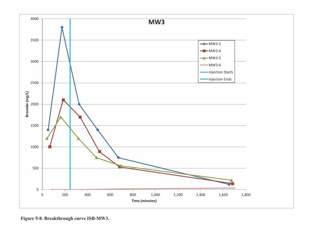
0
500
1000
1500
2000
2500
3000
3500
4000
0 200 400 600 800 1,000 1,200 1,400 1,600 1,800
Brom
ide
(mg/
L)
Time (minutes)
MW3
MW3-3
MW3-4
MW3-5
MW3-6
Injection Starts
Injection Ends
Figure 5-8. Breakthrough curve ISB-MW3.
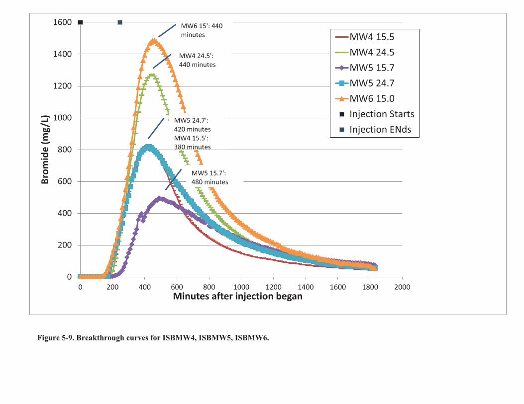
0
200
400
600
800
1000
1200
1400
1600
0 200 400 600 800 1000 1200 1400 1600 1800 2000
Brom
ide
(mg/
L)
Minutes after injection began
MW4 15.5MW4 24.5MW5 15.7MW5 24.7MW6 15.0Injection StartsInjection ENds
MW6 15': 440 minutes
MW4 24.5': 440 minutes
MW5 24.7': 420 minutes MW4 15.5': 380 minutes
MW5 15.7': 480 minutes
Figure 5-9. Breakthrough curves for ISBMW4, ISBMW5, ISBMW6.

Section 5 • Test Design
50
ESTCP ER-0719 Final Report
the seepage velocities calculated for the groundwater tracer test must be corrected for ambient hydraulic gradient conditions. The correction is derived as follows:
During the groundwater tracer test:
V tracer test = K * I tracer test [Equation 1] ne
During ambient conditions: V ambient = K * I ambient
ne
By substitution: V ambient = V tracer test * I ambient [Equation 2] I tracer test
Where:
V = seepage velocity
K = hydraulic conductivity
I = horizontal hydraulic gradient
ne = effective porosity
As discussed in the previous section, the hydraulic gradient induced by an injection at the ISB test cell was evaluated during the January 29, 2010 whey injection event. The average horizontal hydraulic gradient during the ISB cell tracer test was approximated in the vicinity of each of the ISB cell MWs based on the amount of groundwater mounding observed during the January 29, 2010 whey injection event.
Table 5-7 lists the estimated groundwater seepage velocities for ambient conditions, which were calculated using Equation 2 and the hydraulic gradients that were assumed for the tracer injection event. The seepage velocities under ambient (i.e. non-injection) conditions within the ISB test cell are estimated to range from 27 to 82 ft/day.
Hydraulic Conductivity The hydraulic conductivity for each groundwater monitoring point within the ISB test cell was calculated using Equation 1, shown in the previous section. The groundwater seepage velocity and hydraulic gradient during the tracer test were used for this calculation. Table 5-7 lists the calculated hydraulic conductivities. The calculated hydraulic conductivity ranged from 397 ft day to 1,197 ft/day. Depth discrete conductivity values measured for ISB- MW1 and ISB-MW2 were averaged and used for mass discharge calculations. ISB-MW 3 values were not included because the tracer arrival time occurred before the tracer injection was complete.

Section 5 • Test Design
51 ESTCP ER-0719 Final Report
5.2.5 Hydraulic Characterization: ZVI Test Cell A tracer study was also conducted at the ZVI test cell just prior to injection of ZVI to evaluate the injection hydraulic response, finalize ZVI injection parameters, and to evaluate groundwater flow velocity through elution monitoring. Results of the ZVI tracer test are discussed in conjunction with the ZVI injection results in Section 5.5.2 (see also Truex et al. 2010).
5.3 Laboratory Study Results The laboratory tests were conducted to 1) finalize selection of the polymer as the delivery mechanism for the ZVI, 2) determine injection parameters (i.e., quantity of ZVI/polymer addition), and 3) provide baseline reaction kinetics to assist in field data interpretation. The laboratory tests demonstrated that SlurryPro™ does not impact the dechlorination rate of TCE by ZVI in the presence of site sediments. It was observed that zero-order reaction rates in SlurryPro™ range from about 80 to over 100% of the rates in water. Thus, the impact of SlurryPro™ on the ZVI reactions is deemed to be minimal (Truex et al. 2011; see also treatability test in Appendix B). Additionally, the laboratory tests demonstrated that the solubility of TCE is not impacted by SlurryPro™ (Truex et al. 2010). For treatments containing site sediments, reaction rates at 40oC are about 2.5 to 4 times faster than rates at 20oC. As such, the reaction rate is expected to be significantly enhanced by the heating process during the field test. The full treatability test report is provided in Appendix B.
During installation of field test site wells, sediment samples from three of the wells were analyzed for TCE. The mass of TCE within the targeted ZVI treatment zone was estimated to be 2 to 6 kg-TCE. The lower estimate assumes that the TCE concentration measured at the injection well applies to a radius of 1 m from the injection well (220 mg/kg) and that the concentrations measured at MW1 (1.6 mg/kg) and MW2 (11 mg/kg) apply to the remainder of the volume. The high estimate applies the average concentration of the three measurements across the entire treatment volume. While sediment samples were not collected from all of the wells, screening of sediment samples during drilling using a field instrument suggest that the highest TCE concentration is centered around the injection well and that concentrations are lower at the other well locations and likely similar to the concentrations measured at MW1 and MW2.
Results of laboratory treatability tests (ER-0719 project report submitted in October 2008) were used as input to select the ZVI mass to be injected into the test cell. The factors considered for selection included 1) the observed stoichiometry of TCE degraded per mass of ZVI from laboratory treatability tests, 2) the ratio of TCE concentration to ZVI concentration expected in the groundwater within the test zone and how this ratio compares to the ratio in the laboratory treatability tests that were used to determine the TCE degradation rate, 3) the required weight percentage of ZVI in the injection solution and how this percentage compares to the previous tests for ZVI injection and transport (Oostrom et al., 2007), and 4) the material cost of ZVI per treatment volume. Table 5-8 shows the estimated required mass of ZVI in the treatment zone based on the average and maximum stoichiometry observed in the laboratory treatability tests.

Section 5 • Test Design
52
ESTCP ER-0719 Final Report
Table 5-8. Estimated ZVI injection based on laboratory measured stoichiometry of TCE degraded per ZVI mass.
TCE mass (kg) Required ZVI (kg) using average stoichiometry (0.012)
Required ZVI (kg) using maximum stoichiometry (0.034)
2 160 60
Based on this information, a target ZVI injection of 150 kg was selected. This mass of ZVI is sufficient for the estimate of total TCE mass in the treatment zone.
Table 5-9 shows the selected 150-kg ZVI mass in terms of the ratio of TCE to ZVI concentrations in the pore water for comparison to the laboratory treatability test ratios. The field ratio is based on an expected TCE concentration of 10 mg/L in the pore water. During previous full-scale thermal treatment at EGDY, the groundwater TCE concentration increased to between 5 and 10 ppm when subsurface temperatures were increased to between 40 and 60oC. Thus, similar pore water concentrations of TCE were expected when the subsurface is heated during the demonstration.
Table 5-9. Concentration ratios for TCE and ZVI in laboratory tests compared to the selected ZVI injection for the field test.
Test TCE
concentration (mg/L)
ZVI concentration
(g/L)
Ratio of TCE to ZVI concentration
(mg/g) High TCE laboratory 1000 200 5
Low TCE laboratory 100 200 0.5 Field Test with 150 kg ZVI injected 10 13 0.75
5.4 Design and Layout of Technology Components 5.4.1 ISB Field Test Design ISB Test Cell Layout The ISB test cell location was selected at the Fort Lewis Landfill 2 site based on the pre-characterization data collected during the Phase 1 of this demonstration, which revealed that this area contains soil concentration of TCE indicative of residual saturation. The target treatment depth of 9 ft to 20 ft bgs was selected based on the soil coring data which indicated that much of the source material was located at this depth interval in the saturated zone. The test cell wells were installed (as detailed in Table 5-10), and the well configuration, as surveyed by the U.S. Army Corps of Engineers (USACE) Seattle District, is illustrated in Figure 5-5. The test cell was aligned northeast to southwest; approximately parallel to the estimated (not actual) direction

Section 5 • Test Design
53 ESTCP ER-0719 Final Report
Table 5-10. Details of completed wells within ISB test cell. Well ID Date Installed Well Diameter (inches) Screen Interval (ft bgs)
ISB-INJ 11/19/2008 4 9 - 19 ISB-MW1 8/22/2008 1.7 7,12,17,22,27 ISB-MW2 8/20/2008 1.7 7,12,17,22,27 ISB-MW3 8/21/2008 1.7 7,12,17,22,27 ISB-MW4 11/20/2008 2 9 - 24 ISB-MW5 11/20/2008 2 10 - 25 ISB-MW6 11/20/2008 2 9- 24
of groundwater flow as shown in Figure 5-5. Groundwater flow direction at the time of well installation was controlled by the nearby pump-and-treat system to an azimuth of about 233 degrees. During the test, however, several of the well pumps in this system failed and the average groundwater direction during the test changed to an azimuth of 294 degrees. The test cell was comprised of an injection well (ISB-INJ) and six downgradient MWs (ISB-MW1 through ISB-MW6).
ISB Field Injection Equipment During the injections, the injection hose was placed in the injection well ISB-INJ at an approximate depth of 15 ft bgs. An in-line, spring-loaded flow meter and a digital flow totalizer were used to measure injection rates. Depth to groundwater measurements at the injection well and flow readings at the flow meter and totalizer were recorded throughout the injection events and recorded on an amendment injection log. The feed-water for all injections was obtained from 2-inch diameter discharge ports (FX-01 and FX-02) located on the groundwater conveyance line of the Landfill 2 pump and treat system. The discharge ports were equipped with valves and the groundwater was conveyed from the discharge ports to the injection site using ¾-inch diameter rubber hoses. The TCE concentration in the feed-water was approximately 150 microgram per liter (µg/L), based on a sample collected at the conveyance line during the injection.
5.4.2 ZVI Field Test Design ZVI Test Cell Layout The ZVI test design is described in Truex et al. (2010 and 2011) and summarized here. The project test cell was located within JBLM Landfill 2 in a region where TCE had been disposed to surface trenches in quantities sufficient to migrate through the shallow vadose zone (~9 ft thick) and into the top portion of the aquifer. The layout of the test cell encompassed a targeted ZVI treatment volume with a 9-12 foot radius that was about 5 ft thick (approximately 10 to 15 ft bgs) (Figure 5-10). The test cell was comprised of one groundwater injection well and nine MWs nominally screened within the upper Steilacoom Gravel, although some till features are also present within this targeted interval. Groundwater flow direction at the time of well installation was controlled by the nearby pump-and-treat system to an azimuth of about 233 degrees. During the test, however, several of the well pumps in this system failed and the average groundwater
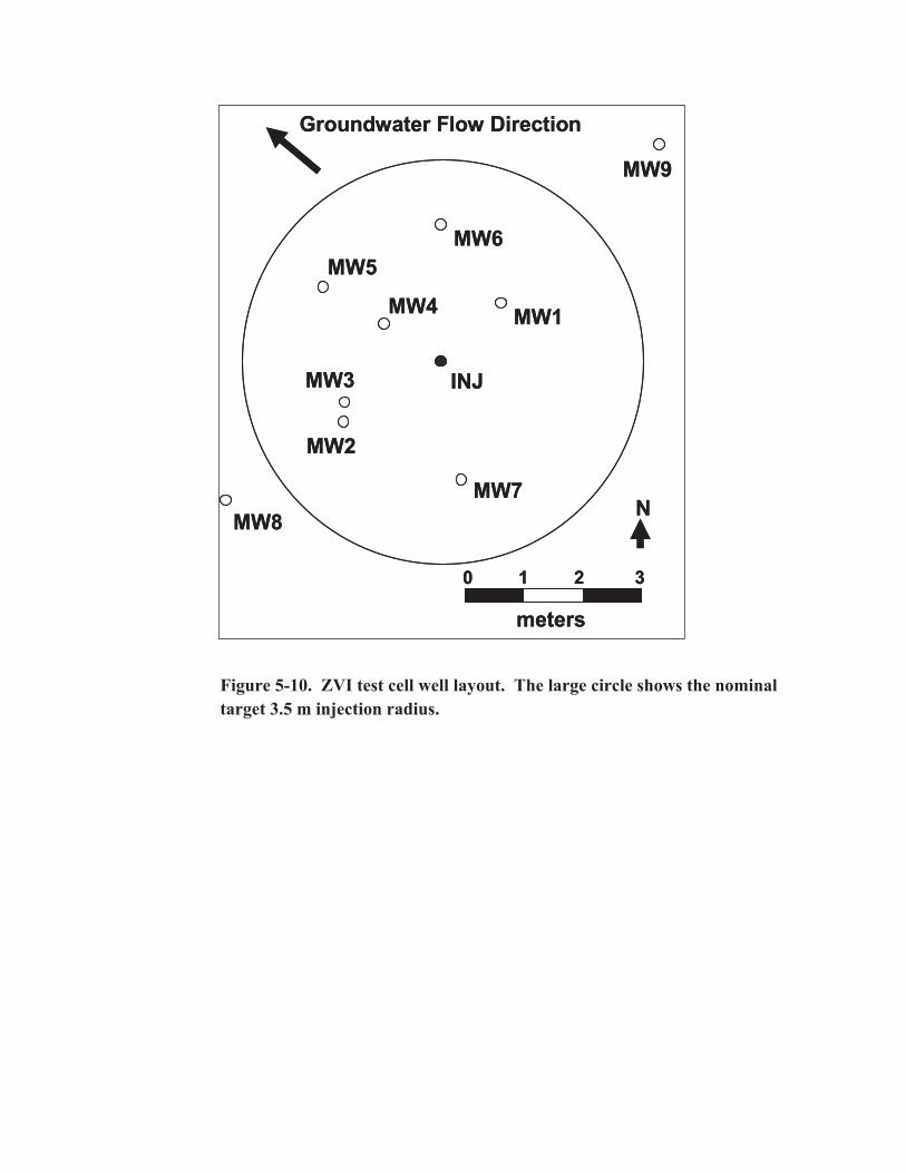
Figure 5-10. ZVI test cell well layout. The large circle shows the nominal target 3.5 m injection radius.
INJ
MW1
MW2
MW3
MW4
MW5MW6
MW7MW8
MW9
0 1 2 3
meters
N
Groundwater Flow Direction
INJ
MW1
MW2
MW3
MW4
MW5MW6
MW7MW8
MW9
0 1 2 3
meters
N
Groundwater Flow Direction
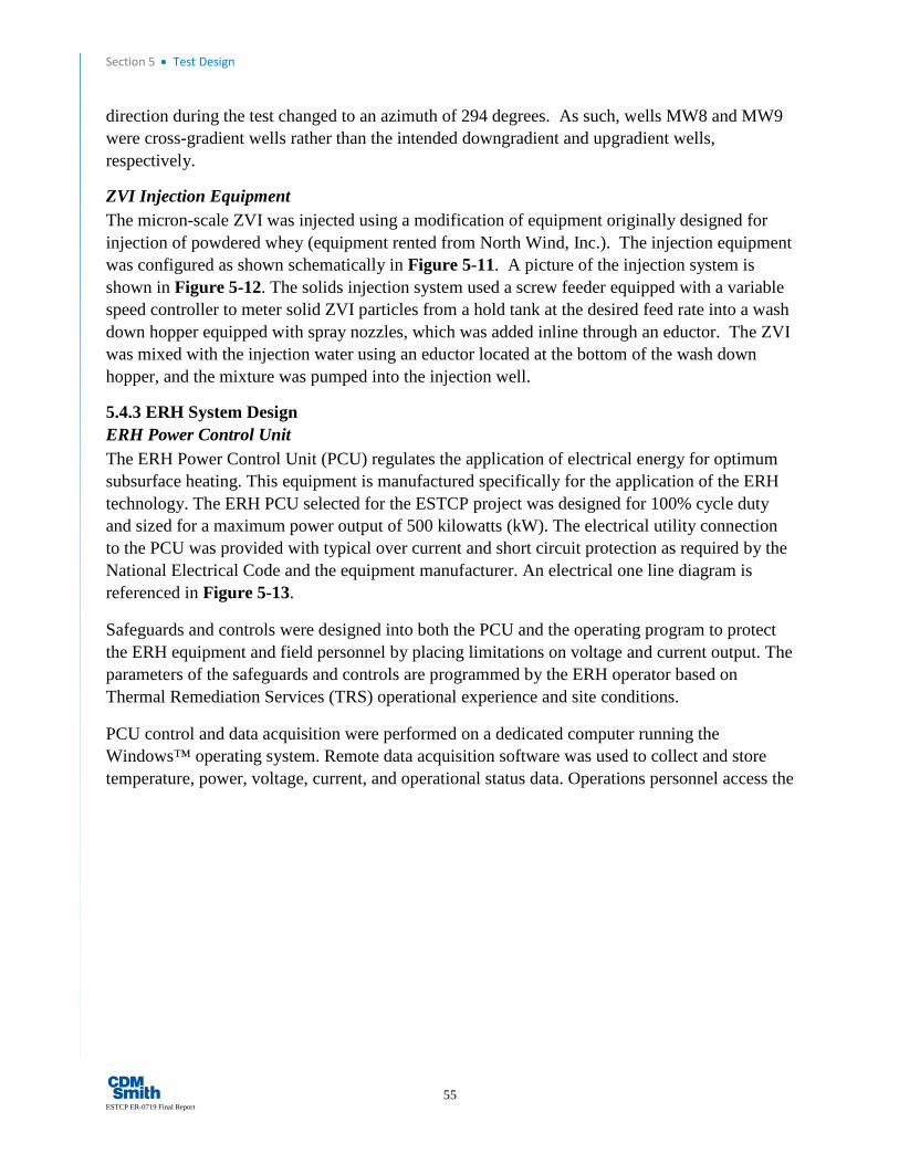
Section 5 • Test Design
55 ESTCP ER-0719 Final Report
direction during the test changed to an azimuth of 294 degrees. As such, wells MW8 and MW9 were cross-gradient wells rather than the intended downgradient and upgradient wells, respectively.
ZVI Injection Equipment The micron-scale ZVI was injected using a modification of equipment originally designed for injection of powdered whey (equipment rented from North Wind, Inc.). The injection equipment was configured as shown schematically in Figure 5-11. A picture of the injection system is shown in Figure 5-12. The solids injection system used a screw feeder equipped with a variable speed controller to meter solid ZVI particles from a hold tank at the desired feed rate into a wash down hopper equipped with spray nozzles, which was added inline through an eductor. The ZVI was mixed with the injection water using an eductor located at the bottom of the wash down hopper, and the mixture was pumped into the injection well.
5.4.3 ERH System Design ERH Power Control Unit The ERH Power Control Unit (PCU) regulates the application of electrical energy for optimum subsurface heating. This equipment is manufactured specifically for the application of the ERH technology. The ERH PCU selected for the ESTCP project was designed for 100% cycle duty and sized for a maximum power output of 500 kilowatts (kW). The electrical utility connection to the PCU was provided with typical over current and short circuit protection as required by the National Electrical Code and the equipment manufacturer. An electrical one line diagram is referenced in Figure 5-13.
Safeguards and controls were designed into both the PCU and the operating program to protect the ERH equipment and field personnel by placing limitations on voltage and current output. The parameters of the safeguards and controls are programmed by the ERH operator based on Thermal Remediation Services (TRS) operational experience and site conditions.
PCU control and data acquisition were performed on a dedicated computer running the Windows™ operating system. Remote data acquisition software was used to collect and store temperature, power, voltage, current, and operational status data. Operations personnel access the

ZVI Field Injection Equipment
Figure 5-11. Test equipment schematic.
P&T systemmanifold
Surfactant
ZVI feedeductor system
SlurryPro
In-line turbineflow meter
In-line mixer
1.5 m
2.4 m Inflatable packer
4” well
Sample port
9
Surfactant feed
ZVI solids feed
Eductor to entrain solids in injection fluid
Static mixer
Static mixer
SlurryPro feed
Injection fluid sample port
Washdown hopper
Surfactant metering pump
Figure 5-12. ZVI Injection System.
110

Figure 5-13. Power Control Unit (PCU) Electrical One-Line Drawing.
Section 5 • Test Design
59 ESTCP ER-0719 Final Report
data acquisition system to download data, or monitor and control the ERH process either directly or by remote connection.
Each ERH application is designed to perform in the specific soil and groundwater properties encountered at the site. The ERH PCU is equipped to handle a wide range of electrical conductivity conditions in the subsurface.
ERH Electrode Layout Both the ISB and ZVI test cells employed 7 electrodes each located as shown in Figure 5-14 and Figure 5-15 respectively. Each electrode location consisted of a single 12-foot electrode element which is connected to the surface via a high temperature electrical cable.
The ERH electrodes are simply devices used to transfer electrical energy to subsurface soil and groundwater. Relatively speaking, there is no radius of influence with respect to temperature associated with an individual electrode. It is best to consider the entire electrode array when considering the radius of thermal influence. During ERH, the primary in situ heating mechanism is the resistance to electrical current flow in the soil and groundwater being treated and is not the thermal conductivity from heat generated at the electrode.
Electrical current flows in all directions from each electrode borehole, but is most strongly directed to adjacent electrodes of a different electrical phase. The electrical current exits the borehole radially, and then bends towards the nearest electrode. This radial travel allows for heating a certain distance away from each border electrode at the perimeter of the electrode array. The distance is estimated to be slightly less than one-half the distance between electrodes of a different phase. Field observations have confirmed this to be a reliable estimate of the radius of active heating.
Both the ISB and ZVI test cell electrodes were installed within a 12-inch diameter electrode borehole to a depth of approximately 20-ft bgs. The annular space surrounding the electrically conductive interval of the electrodes (from 8 to 20-ft bgs) was filled with TRS’ patented conductive backfill to transfer electrical current to the treatment volume. In the shallow portion, where the electrode is not electrically conductive, (0 to 8-ft bgs), the annular space was filled with non-conductive materials such as native soil or neat cement grout. Electrode completion details are provided in Figure 5-16.
Electrodes were positioned at an average spacing of 11.5-ft on center to allow the optimal energy application that would provide the required subsurface temperatures without the formation of steam at the electrodes.. The electrode spacing was determined by a number of factors unique to the EGDY and this project including soil type, geometry of the treatment area, groundwater elevation and flux, groundwater conductivity, depth of treatment, the total organic carbon (TOC) content of soil in the treatment area, and the distribution, concentration, and clean-up goals of the contamination to be treated, to name a few. Electrode spacing was also determined based on a balance of power, they key consideration for managing temperatures. For each kW of power applied to the site, a small percentage is lost to the subsurface surrounding the treatment volume.

Figure 5-14. ERH Electrode Locations of the ISB Test Cell.

Figure 5-15. ERH Electrode Locations of the ZVI Test Cell.
113
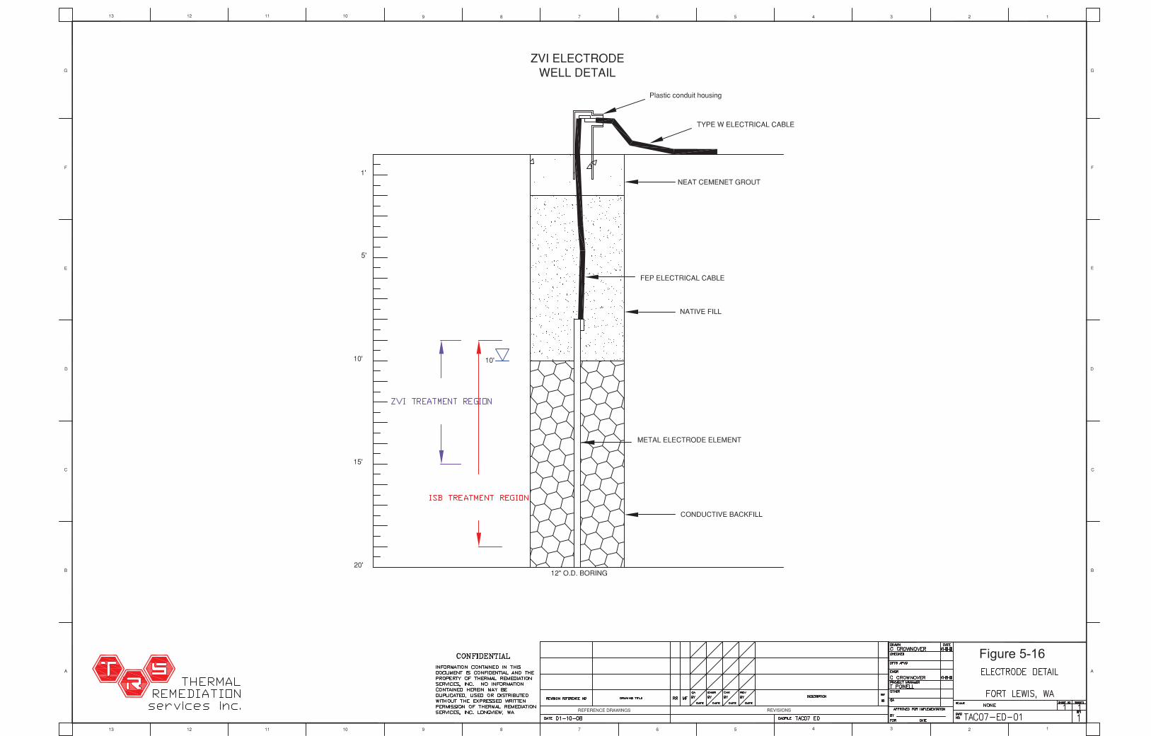
114
Figure 5-16
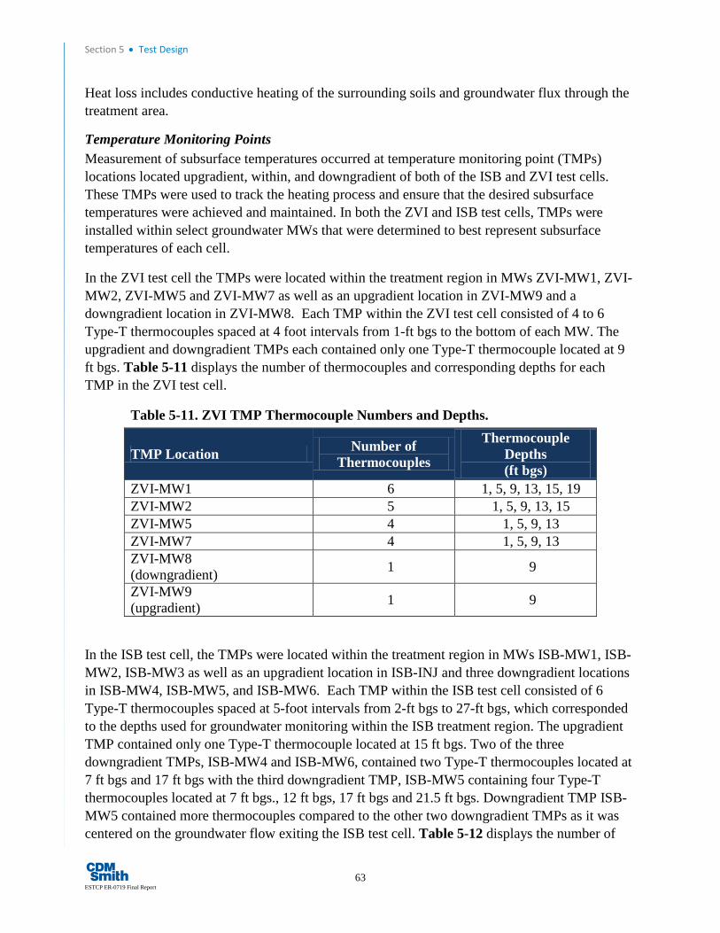
Section 5 • Test Design
63 ESTCP ER-0719 Final Report
Heat loss includes conductive heating of the surrounding soils and groundwater flux through the treatment area.
Temperature Monitoring Points Measurement of subsurface temperatures occurred at temperature monitoring point (TMPs) locations located upgradient, within, and downgradient of both of the ISB and ZVI test cells. These TMPs were used to track the heating process and ensure that the desired subsurface temperatures were achieved and maintained. In both the ZVI and ISB test cells, TMPs were installed within select groundwater MWs that were determined to best represent subsurface temperatures of each cell.
In the ZVI test cell the TMPs were located within the treatment region in MWs ZVI-MW1, ZVI-MW2, ZVI-MW5 and ZVI-MW7 as well as an upgradient location in ZVI-MW9 and a downgradient location in ZVI-MW8. Each TMP within the ZVI test cell consisted of 4 to 6 Type-T thermocouples spaced at 4 foot intervals from 1-ft bgs to the bottom of each MW. The upgradient and downgradient TMPs each contained only one Type-T thermocouple located at 9 ft bgs. Table 5-11 displays the number of thermocouples and corresponding depths for each TMP in the ZVI test cell.
Table 5-11. ZVI TMP Thermocouple Numbers and Depths.
TMP Location Number of Thermocouples
Thermocouple Depths (ft bgs)
ZVI-MW1 6 1, 5, 9, 13, 15, 19 ZVI-MW2 5 1, 5, 9, 13, 15 ZVI-MW5 4 1, 5, 9, 13 ZVI-MW7 4 1, 5, 9, 13 ZVI-MW8 (downgradient) 1 9
ZVI-MW9 (upgradient) 1 9
In the ISB test cell, the TMPs were located within the treatment region in MWs ISB-MW1, ISB-MW2, ISB-MW3 as well as an upgradient location in ISB-INJ and three downgradient locations in ISB-MW4, ISB-MW5, and ISB-MW6. Each TMP within the ISB test cell consisted of 6 Type-T thermocouples spaced at 5-foot intervals from 2-ft bgs to 27-ft bgs, which corresponded to the depths used for groundwater monitoring within the ISB treatment region. The upgradient TMP contained only one Type-T thermocouple located at 15 ft bgs. Two of the three downgradient TMPs, ISB-MW4 and ISB-MW6, contained two Type-T thermocouples located at 7 ft bgs and 17 ft bgs with the third downgradient TMP, ISB-MW5 containing four Type-T thermocouples located at 7 ft bgs., 12 ft bgs, 17 ft bgs and 21.5 ft bgs. Downgradient TMP ISB-MW5 contained more thermocouples compared to the other two downgradient TMPs as it was centered on the groundwater flow exiting the ISB test cell. Table 5-12 displays the number of
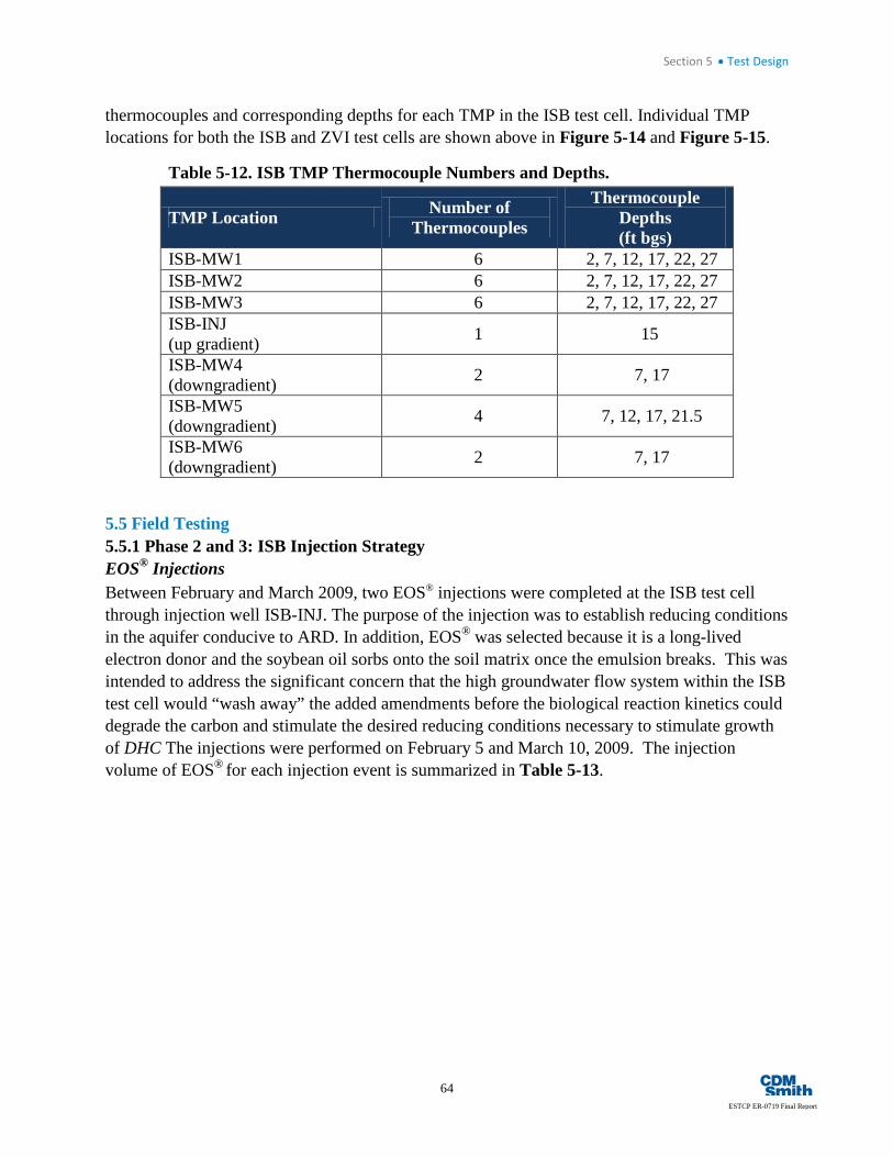
Section 5 • Test Design
64
ESTCP ER-0719 Final Report
thermocouples and corresponding depths for each TMP in the ISB test cell. Individual TMP locations for both the ISB and ZVI test cells are shown above in Figure 5-14 and Figure 5-15.
Table 5-12. ISB TMP Thermocouple Numbers and Depths.
TMP Location Number of Thermocouples
Thermocouple Depths (ft bgs)
ISB-MW1 6 2, 7, 12, 17, 22, 27 ISB-MW2 6 2, 7, 12, 17, 22, 27 ISB-MW3 6 2, 7, 12, 17, 22, 27 ISB-INJ (up gradient) 1 15
ISB-MW4 (downgradient) 2 7, 17
ISB-MW5 (downgradient) 4 7, 12, 17, 21.5
ISB-MW6 (downgradient) 2 7, 17
5.5 Field Testing 5.5.1 Phase 2 and 3: ISB Injection Strategy EOS® Injections Between February and March 2009, two EOS® injections were completed at the ISB test cell through injection well ISB-INJ. The purpose of the injection was to establish reducing conditions in the aquifer conducive to ARD. In addition, EOS® was selected because it is a long-lived electron donor and the soybean oil sorbs onto the soil matrix once the emulsion breaks. This was intended to address the significant concern that the high groundwater flow system within the ISB test cell would “wash away” the added amendments before the biological reaction kinetics could degrade the carbon and stimulate the desired reducing conditions necessary to stimulate growth of DHC The injections were performed on February 5 and March 10, 2009. The injection volume of EOS® for each injection event is summarized in Table 5-13.
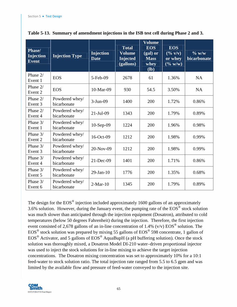
Section 5 • Test Design
65 ESTCP ER-0719 Final Report
Table 5-13. Summary of amendment injections in the ISB test cell during Phase 2 and 3.
Phase/ Injection Event
Injection Type Injection Date
Total Volume Injected (gallons)
Volume EOS
(gal) or Mass whey (lb)
EOS (% v/v) or whey (% w/w)
% w/w bicarbonate
Phase 2/ Event 1 EOS 5-Feb-09 2678 61 1.36% NA
Phase 2/ Event 2 EOS 10-Mar-09 930 54.5 3.50% NA
Phase 2/ Event 3
Powdered whey/ bicarbonate 3-Jun-09 1400 200 1.72% 0.86%
Phase 2/ Event 4
Powdered whey/ bicarbonate 21-Jul-09 1343 200 1.79% 0.89%
Phase 3/ Event 1
Powdered whey/ bicarbonate 10-Sep-09 1224 200 1.96% 0.98%
Phase 3/ Event 2
Powdered whey/ bicarbonate 16-Oct-09 1212 200 1.98% 0.99%
Phase 3/ Event 3
Powdered whey/ bicarbonate 20-Nov-09 1212 200 1.98% 0.99%
Phase 3/ Event 4
Powdered whey/ bicarbonate 21-Dec-09 1401 200 1.71% 0.86%
Phase 3/ Event 5
Powdered whey/ bicarbonate 29-Jan-10 1776 200 1.35% 0.68%
Phase 3/ Event 6
Powdered whey/ bicarbonate 2-Mar-10 1345 200 1.79% 0.89%
The design for the EOS® injection included approximately 1600 gallons of an approximately 3.6% solution. However, during the January event, the pumping rate of the EOS® stock solution was much slower than anticipated through the injection equipment (Dosatron), attributed to cold temperatures (below 50 degrees Fahrenheit) during the injection. Therefore, the first injection event consisted of 2,678 gallons of an in-line concentration of 1.4% (v/v) EOS® solution. The EOS® stock solution was prepared by mixing 55 gallons of EOS® 598 concentrate, 1 gallon of EOS® Activator, and 5 gallons of EOS® AquaBupH (a pH buffering solution). Once the stock solution was thoroughly mixed, a Dosatron Model DI-210 water–driven proportional injector was used to inject the stock solutions for in-line mixing to achieve the target injection concentrations. The Dosatron mixing concentration was set to approximately 10% for a 10:1 feed-water to stock solution ratio. The total injection rate ranged from 5.5 to 6.5 gpm and was limited by the available flow and pressure of feed-water conveyed to the injection site.

Section 5 • Test Design
66
ESTCP ER-0719 Final Report
The second injection event consisted of 930 gallons of an in-line concentration of 3.5 % (v/v) EOS® solution. The EOS® stock solution was prepared by mixing 55 gallons of EOS® 598 concentrate, 1 gallon of EOS® Activator, and 5 gallons of EOS® AquaBupH (a pH buffering solution). An EOS® stock solution was directly pumped into the injection well using a submersible pump and manifold. The target injection concentration was achieved using this revised approach.
Bicarbonate Buffered Whey Injections Results of the EOS® injections suggested that the EOS® was not retained within the test cells following either EOS® injection in sufficient quantity to drive conditions anaerobic. Therefore, a decision to switch from EOS® to buffered whey injection was made. During the ER-0218 demonstration, whey powder was used and was successful at achieving sufficiently reducing conditions to stimulate growth of Dehalococcoides and achieve reduction of chlorinated ethenes (Lee et al 2008, 2012). However, fermentation of whey powder also significantly reduced pH, which resulted in a reduction in dechlorination rate and efficiency. Therefore, between June 2009 and September 2010, three sodium bicarbonate-buffered, whey injections were completed at the ISB-INJ well for Phase 2 (Table 5-13), and six sodium bicarbonate-buffered, whey injections were completed at the ISB-INJ well for Phase 3 between September 2009 and March 2010. The injection volume and mass of whey and sodium bicarbonate for each injection event is summarized in Table 5-13.
Each injection event consisted of approximately 1,000 gallons of whey solution; immediately followed by 200 gallons of sodium bicarbonate solution. At the end of each injection, 200 gallons of water were injected into the well to flush the screen and filter pack. The total target in situ amendment concentration was approximately 1.8% (w/w) whey and 0.9% (w/w) bicarbonate.
The whey injections consisted of first preparing a concentrated stock solution by mixing 200 lbs of cheese whey powder with 100 gallons of water. The stock solution was prepared and mixed in 55-gallon drums using mixing sticks and recirculation with a submersible sump pump. A Dosatron Model DI-210 water–driven proportional injector was used to inject the stock solution with a larger volume of water to achieve the target concentration. The Dosatron mixing concentration was set to approximately 10% for a 10:1 feed-water to stock solution ratio. The whey solution injection rate ranged from 5 to 6 gpm and was limited by the available flow and pressure of the feed-water conveyed to the injection site. The sodium bicarbonate injections consisted of preparing a concentrated stock solution by mixing a total of 100 lbs of No. 2 sodium bicarbonate with 200 gallons of water. The solution was prepared in 55-gallon drums and mixed via recirculation with a submersible sump pump. After the sodium bicarbonate was completely dissolved, the solution was injected into the well using the sump pump. Sodium bicarbonate injection rates ranged from 6 to 9 gpm.
5.5.2 Phase 2 and 3: ZVI Injection Strategy A full description of the ZVI injection process is described in Truex et al. 2010 and is summarized here. Prior to ZVI injection, a sodium bromide (100 mg/L as bromide ion) solution

Section 5 • Test Design
67 ESTCP ER-0719 Final Report
was injected to evaluate the injection pressure, bromide distribution within the targeted test zone, and to enable monitoring of bromide elution to estimate the groundwater velocity at the test site. Tracer concentrations were monitored in the test cell wells using a downhole bromide ion selective electrode during and after injection to define the tracer breakthrough and elution responses within each of the MWs ZVI-MW1 through MW9. Tracer breakthrough (50% of injected concentration) was compared to the predicted radial transport for flow within a cylinder with a height equal to the well screen length and a porosity of the outwash material. Tracer elution (time for reduction to 50% of peak concentration) was evaluated for MWs ZVI-MW1 through -MW7 to estimate groundwater velocity based on advection of clean water upgradient of the well estimated based on a nominal injection radius of 3 m and a groundwater flow direction of 294 degrees.
The ZVI injection system described in Section 5.4.2 was used to inject a solution consisting of 0.02 wt% SlurryPro™ (SlurryPro CDP, KB International, www.kbtech.com), 0.0008 wt% surfactant (Aerosol, Sigma Chemical, St. Louis, Missouri), 1.36 wt% S-3700 ZVI (Fe0 colloids with a diameter of 2 +/- 1 um, International Specialty Products, Wayne, New Jersey), and groundwater from the influent line of the Landfill 2 pump and treat system, which contained a nominal TCE concentration of 150 ug/L. The injection system was used to feed ZVI at a nominal rate of 1.1 kg/min into the injection water. Surfactant from a 1 wt% stock solution was metered into the wash down hopper portion of the ZVI solids feed system to disperse the ZVI particles and prevent clumping.
A 0.2 wt% SlurryPro™ stock solution (Figure 5-17) was metered into the injection water downstream of the ZVI/surfactant feed system. The SlurryPro™ component of the injection solution was selected because its rheological properties as a shear-thinning fluid facilitate ZVI transport through porous media (Oostrom et al. 2007). The injection system provided a continuous flow method for preparing a suitable, uniformly-mixed injection solution (Figure 5-11). Figure 5-18 shows a picture of the ZVI injection solution and Figure 5-19 shows groundwater samples containing ZVI collected from the MWs at the mid-point of ZVI injection.
5.5.3 Phase 3: ERH System Operations The ERH operations period for Phase 3 of the ESTCP ER-0719 remediation includes site activities from system shakedown and start-up through ERH operations and system demobilization.
ERH System Start Up ERH system shakedown and start-up testing began the week of June 8, 2009. With all electrical and temperature monitoring installations complete, proper operation of the internal and external interlocks for each system component was verified. TRS then applied power to the electrodes for start-up voltage testing on June 16, 2009.
Concurrent with the ERH system testing, step and touch voltage safety tests were also performed. These tests are done to evaluate surface conditions for the presence of induced voltages. Areas where personnel may walk or touch surfaces are measured for voltage potential.

Figure 5-17. Stock solution of SlurryPro™ (0.2 wt%).
115

Figure 5-18. Picture of ZVI injection solution during injection.
116
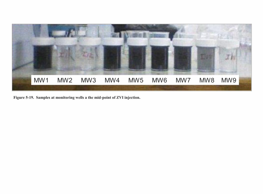
MW1 MW2 MW3 MW4 MW5 MW6 MW7 MW8 MW9
Figure 5-19. Samples at monitoring wells a the mid-point of ZVI injection.
117

Section 5 • Test Design
71 ESTCP ER-0719 Final Report
Any areas with measurements of 15 volts are identified and the situation rectified by either isolation, or bonding. During this procedure the step and touch voltage testing verified that no locations exceeded the 15-Volt standard.
With the initial surface voltage survey complete, the applied voltage to the subsurface was slowly increased over the remainder of the start-up period. At each voltage increase, checks for surface voltage were performed and results recorded until the final start-up voltage of 325 volts was reached. In no instance did step-and-touch readings at the surface exceed the TRS 15-volt limit. The ERH system first operated overnight in unattended mode on June 17, 2009 and that date was set as the start of the operations period.
Safety and Security During ERH start-up, and throughout system operation, step-and-touch voltage potentials in and around the electrode field were monitored frequently to ensure public and worker safety. At no time during ERH system start-up or operations were surface voltages above 15-volts measured at any location on or adjacent to the electrode field. During ERH operations the remediation area was also surrounded by security fencing and access to the remediation area was not permitted unless proper Lock-Out/Tag-Out (LOTO) procedures were followed prior to access by project team members.
A LOTO procedure was established by TRS during active ERH heating to ensure the safety of all ESTCP team members while conducting field work within the ER-0719 test cells during Phase 3 of operations. Prior to conducting any field activities within the treatment region ERH power application was ceased and zero energy application was verified by TRS. The PCU was locked out using a keyed LOTO device by on site personnel conducting the field work and was only unlocked after field work was completed and the treatment region was cleared of all personnel. Power was only able to be reapplied to the treatment region after all site personnel were verified out of the treatment region and the PCU LOTO device was unlocked.
ERH Operations Treatment of the ZVI test cell began on June 17, 2009 with a target treatment temperature of 50°C, however, modification were made throughout the test based on analytical results. The actual average temperatures in the ZVI test cell ranged from 35 and 48°C from August 20, 2009 through December 31, 2009. From January 1, 2010 through the end of treatment on March 22, 2010 temperatures in the ZVI cell were maintained between 31 and 34°C. During this period a total of 60,038 kilowatt hour (kWh) of energy was applied to the ZVI treatment region.
Treatment of the ISB test cell began on September 26, 2009 with a target treatment temperature of 40°C. The ISB test cell achieved an average temperature of between 30 and 48°C from October 12, 2009 through January 3, 2010. From January 4, 2010 through February 10, 2010 temperatures in the ISB cell were maintained between 25 and 30°C. From February 11, 2010 through the end of treatment on March 22, 2010 temperatures in the ISB cell were maintained between 29 and 36°C. During this period total of 33,330kWh of energy was applied to the ISB treatment region.
Section 5 • Test Design
72
ESTCP ER-0719 Final Report
ERH Operations System Optimization The ERH system was continuously monitored which allowed operational adjustments to be made either remotely or by on-site staff. The ability to make changes to system operations remotely helped ensure that the remedial objectives of the project were met while the system remained safe and environmentally compliant. Through the use of remote monitoring of the temperature monitoring system and remote operating features of the power output control systems, operations personnel were able to respond rapidly to system changes and maximize energy input to both the ISB and ZVI test cells concurrently.
TRS used voltage adjustment and on-time as the two primary methods of optimization during the treatment of both test cells. The soil conductivity at each electrode was unique to that location. TRS overcame the unique conductivities at each electrode by varying the applied voltage. Conductivities changed throughout the treatment duration, so frequent monitoring and adjustments were necessary. TRS also used ERH power application “on-time” as a method to maintain optimal treatment temperatures for each cell. Once the target temperature range had been met, power could be turned off to prevent overheating the soils, and wasting energy or reducing treatment effectiveness. The amount of on-time necessary to maintain temperatures was adjusted by observing the daily temperature data.
Demobilization The electrodes were de-energized and the electrical service was permanently locked out on March 22, 2010. Final system demobilization, equipment breakdown, and material packaging were complete by May 18, 2010 and the PCU was removed from the site on May 19, 2010.
The thermocouples were left in their associated MWs for continued monitoring until the wells are permanently abandoned. Post-Phase 3 temperatures were monitored using a hand held thermocouple reader.
The electrodes in both the ZVI and ISB test cells were decommissioned by removal of surface appurtenances upon completion of Phase 3.
5.6 Sampling Methods Samples, including groundwater, soil gas and soils were collected from all three phases in the ZVI and ISB test cell. The total number of samples taken and the types of samples that were collected are summarized in Tables 5-14 and 5-15. Analytical methods are highlighted in Table 5-16.

Section 5 • Test Design
73 ESTCP ER-0719 Final Report
Table 5-14. ZVI Sample Types and Quantities.
Phase Matrix Number of Samples Analytesa, b, c, d Location
Pre-Demonstration Design
Soil Gas (GORETM) 15
VOC, hydrocarbon, ethane, ethene, acetylene
Grid pattern across potential Test Cell location
Groundwater 3 VOC, field parameters INJ, MW1, MW2
Groundwater Continuous until breakthrough
Sodium Bromide
Groundwater Sodium Bromide MW1-MW7
Phase Matrix Number of Samples Analyte Location
Phase 1, Baseline Conditions
Groundwater 20
VOC, dissolved gases, anions, Fe(II), field parameters
INJ, MW1-MW9
Groundwater 2 Microbial Targets MW2, MW4
Soil Gas (Summa) 5 VOC, ethene, ethane, acetylene
MW2, MW4, MW5, MW6, MW7
Soil Gas (GORETM) 6
VOC, hydrocarbon, ethane, ethene, acetylene
MW2, MW4, MW6, Flux A, Flux B, Flux C
Soil 9 VOC Soil Cores near INJ, MW1, MW2

Section 5 • Test Design
74
ESTCP ER-0719 Final Report
Table 5-14. ZVI Sample Types and Quantities. (Continued)
Phase Matrix Number of Samples Analytesa, b, c, d Location
Phase 2, Ambient Temperature
Groundwater 40 VOC, dissolved gases, anions, field parameters
INJ, MW1-MW9
Groundwater 20 Fe(II) INJ, MW1-MW9
Groundwater 2 Microbial Targets MW2, MW4
Soil Gas (Summa) 5 VOC, ethene, ethane, acetylene
MW2, MW4, MW5, MW6, MW7
Soil Gas (GORETM) 6
VOC, hydrocarbon, ethane, ethene, acetylene
MW2, MW4, MW6, Flux A, Flux B, Flux C
Soil 6 VOC Soil Cores near INJ, MW1
Phase 3, High Temperature
Groundwater 160 VOC, dissolved gases, anions, field parameters
INJ, MW1-MW9
Groundwater 30 Fe(II) INJ, MW1-MW9
Groundwater 10 Microbial Targets MW2, MW4
Soil Gas (Summa) 35 VOC, ethene, ethane, acetylene
MW2, MW4, MW5, MW6, MW7
Soil Gas (GORETM) 18
VOC, hydrocarbon, ethane, ethene, acetylene
MW2, MW4, MW6, Flux A, Flux B, Flux C
Soil 9 VOC Soil Cores near INJ, MW1, MW2
(a) VOCs to be quantified include PCE, TCE, 1-1,-DCE, cis-DCE, trans-DCE, and VC. (b) Dissolved gases include ethene, ethane, and acetylene. (c) Anions include Cl-, Br-, SO4
2-, F-, and NO3- (d) Field parameters include Br- and/or I- DO, oxidation reduction potential (ORP), conductance, and temperature.

Section 5 • Test Design
75 ESTCP ER-0719 Final Report
Table 5-15. ISB Sample Types and Quantities.
Phase Matrix Number of Samples Analytesa, b, c, d Location
Pre-Demonstration Design
Soil Gas (GORETM) 16
VOC, hydrocarbon, ethane, ethene, acetylene
Grid pattern across potential Test Cell location
Groundwater 9 VOC, field parameters
MW1, MW2, MW3
Groundwater Continuous until breakthrough
Sodium Bromide MW4, MW5, MW6
Groundwater 88 Sodium Bromide MW1-MW6
Phase 1, Baseline Conditions
Groundwater 16
VOC, dissolved gases, FE (II), COD, anions, field parameters
INJ, MW1-MW6
Groundwater 4 Microbial Targets
MW1, MW2, MW3, MW5
Soil Gas (Summa) 3 VOC, ethene, ethane, acetylene
MW1, MW2, MW3
Soil Gas (GORETM) 6
VOC, hydrocarbon, ethane, ethene, acetylene
MW1, MW2, MW3, Flux A, Flux B, Flux C
Soil 9 VOC Soil Cores near INJ, MW1, MW2
Phase 2, Ambient Temperature
Groundwater 78
VOC, dissolved gases, anions, COD, field parameters
INJ, MW1-MW6
Groundwater 52 Fe(II) INJ, MW1-MW6
Groundwater 8 Microbial Targets MW2, MW4
Soil Gas (Summa) 6 VOC, ethene, ethane, acetylene
MW1, MW2, MW3
Soil Gas (GORETM) 24
VOC, hydrocarbon, ethane, ethene, acetylene
MW1, MW2, MW3, Flux A, Flux B, Flux C
Soil 9 VOC Soil Cores near INJ, MW1

Section 5 • Test Design
76
ESTCP ER-0719 Final Report
Table 5-15. ISB Sample Types and Quantities. (Continued)
Phase Matrix Number of Samples Analytesa, b, c, d Location
Phase 3, High Temperature
Groundwater 88
VOC, dissolved gases, anions, COD, field parameters
INJ, MW1-MW6
Groundwater 78 Fe(II) INJ, MW1-MW6
Groundwater 6 Microbial Targets MW2, MW4
Soil Gas (Summa) 11 VOC, ethene, ethane, acetylene
MW1, MW2, MW3
Soil Gas (GORETM) 18
VOC, hydrocarbon, ethane, ethene, acetylene
MW1, MW2, MW3, Flux A, Flux B, Flux C
Soil 9 VOC Soil Cores near INJ, MW1, MW2
(a) VOCs to be quantified include PCE, TCE, cis-DCE, trans-DCE, and VC. (b) Dissolved gases include ethene, ethane, and methane. (c) Anions include Cl-, Br-, SO4
2-, and NO3-. (d) Field parameters include Br- and/or I- and DO, ORP, conductance, temperature, pH and alkalinity.

Table 5-16. Groundwater Sample Analysis Summary.
Matrix Analytes Sample Container
Preservative Analytical Method
Holding Time
ZVI and/or ISB Test Cell
Groundwater
Bromide One 125-mL HDPE
Cool to 4ºC Ion-specific electrode
24 hours ZVI and ISB
VOCs (TCE, DCE isomers, VC)
Three glass 40-mL VOA vials
No headspace, HCl pH<2, cool 4ºC,
SW846-8260b 14 days ZVI and ISB
Dissolved gases (ethene, ethane, methane, acetylene)
Three glass 40-mL VOA vials
HCl pH<2, cool to 4ºC
RSKSOP-175 14 days ZVI and ISB
COD Glass H2SO4 pH<2 EPA 410.2 28 days ISBFerrous Iron 60 ml HDPE - HACH Field
Test Kit- ZVI and ISB
Water Levels In situ - Contractor specific SOP
- ZVI and ISB
Anions (sulfate, nitrate, chloride, sulfide)
Glass or plastic Cool to 4ºC Ion chromatography EPA300.0
28 days ZVI and ISB
Purge parameters, (Temperature, pH, Specific Conductivity, ORP)
Collect during purging in flow-through cell
- Direct Measurement Water Quality Probe
- ZVI and ISB
Microbial Parameters 1 L HDPE Cool to 4ºC qPCR 24 hoursbefore filtering
ZVI and ISB
Soil Gas (Summa) VOCs, dissolved gases
Summa Canister - EPA TO14A 30 day ZVI and ISB
Dissolved gases Summa Canister - ASTM D1946 30 day ZVI and ISB
Soil Gas (GORETM)VOCs, dissolved
gases, hydrocarbonsGORETM Modules
- Modified EPA 8260/8270
- ZVI and ISB
VOCs Glass Cool to 4ºC EPA 8260B 14 days ZVI and ISB
186
Section 5 • Test Design
78
ESTCP ER-0719 Final Report
5.6.1 Tracer Test A tracer test was conducted in both the ZVI and ISB demonstration cells during the pre-characterization phase as discussed in Section 5.2.4 and 5.2.5.
5.6.2 Groundwater Sampling Methods Low-flow groundwater sampling (micropurging) was used for all events to minimize the drawdown on the aquifer. Groundwater samples included water quality parameters (temperature, pH, specific conductivity, oxidation-reduction potential (ORP) and DO), ferrous iron, VOCs, dissolved gases, anions, COD (ISB only) and microbial targets. Water quality parameters were collected and recorded after purging parameters were met (stabilization or purged to dryness twice). The water quality meter was properly calibrated per manufacturer prior to sampling. Ferrous iron was collected and analyzed in field using the HACH field kit. For VOC, dissolved gas, anions and COD, the appropriate sample container, as outlined in Table 5-16, was filled, placed in a cooler with ice and sent to Test America-Tacoma or Idaho State University for analysis. To minimize volatilization during Phase 3 heating, groundwater was passed through stainless steel cooling coils at 20˚C before samples were collected.
5.6.3 Soil Gas Sampling Methods GORETM modules were installed in the pre-characterization phase to identify TCE hot spots in the proposed test cells. The modules were placed in the soil using a rotary hammer drill at a depth of 3-4 ft bgs and deployed for a total of 5 days. Results of the soil gas survey were used to finalize ZVI and ISB demonstration cell locations.
During Phase 1, 2 and 3, soil gas samples were collected using Summa Canisters and/or GORETM modules. All soil gas samples were analyzed for VOCs, ethane, ethene and acetylene. To correlate the Summa and GORETM data, the SV port was purged, GORETM modules were placed in the screened portion of the SV port, the port was sealed from the atmosphere and the module was left for approximately 24 hours. To accommodate for the GORETM modules not fitting into the ZVI SV ports an alternative sampling technique was established. Teflon tubing was inserted into the SV port to a depth of 5 ft bgs. A 500 mL polybottle was attached to the tubing above ground. The GORETM module was placed in the polybottle, the lid was sealed with tape and the module was left for approximately 24 hours. Summa soil gas samples were collected following manufacturer recommendations immediately after the GORETM modules were removed.
GORETM modules were also installed 6” below the soil surface to monitor soil gas flux. Soil gas flux chambers consisted of a 4” diameter PVC pipe approximately 4” long filled with clean sand. The GORETM modules were placed in the flux chamber for a duration of 24 hours during the same time that modules were emplaced in the SV wells. Modules were collected and sent to GORE for analysis of VOCs and dissolved gases.
Following the removal of the GORE™ modules, Summa soil gas samples were collected. For the ISB test cell, the Summa canister tubing was inserted into the screened portion of the port, the top of the port was sealed and the canister was allowed to collect a sample for approximately one
Section 5 • Test Design
79 ESTCP ER-0719 Final Report
hour. In the ZVI test cell, the Summa canister was attached to the dedicated tubing, sealed and sample was collected for approximately one hour.
5.6.4 Soil Sampling Methods Soils were collected in each test cell 3 times, once during borehole installation and once each at the end of Phase 2 and Phase 3. Samples were collected near the same location and depth for every phase to maximize consistency and comparability. The samples were screened on site using a PID probe, visually inspected for NAPL and assessed via oil-in-soil dye test kits and sheen tests. Based on the screening results, three samples were selected from each borehole and sent to the laboratory for VOC analysis.
5.6.5 EEH Sampling Methods Subsurface Temperature Monitoring Subsurface temperatures were measured using thermocouples placed in TMPs located within the ISB and ZVI test cells. The PCU system control program was utilized to continuously monitor each thermocouple temperature value and automatically record all the temperature values three times per day.
Thermocouple design is based on the change of electrical resistance between the connection of dissimilar metals when introduced to a specific range of heat. All thermocouples regardless of the temperature range they are designed for, or Type, are unable to be calibrated. In the rare event of a thermocouple failure the thermocouple will not read a correct value if a value is able to be read at all.
To verify the correct operation of the thermocouples used in both the ZVI and ISB test cells a hand-held thermocouple reader was used to validate and verify that the temperatures recorded using the automated data collection system matched those read using the hand held meter. Thermocouples were verified for correct operation after initial installation, when recorded temperatures appeared to be incorrect, and randomly throughout Phase 3 of operations.
ERH Power Output and Control Monitoring PCU output and control data acquisition was performed on a dedicated computer running the WindowsTM operating system. Remote data acquisition software was used to collect and store power, voltage, current, and operational status data three times per day during Phase 3 of operations. Operations personnel accessed the data acquisition system to download data, or monitor and control the ERH process either directly or by remote connection.
Table 5-17 summarizes all temperature and power output sampling frequency and locations associated with the application of ERH low temperature heating for both the ZVI and ISB treatment regions.

Section 5 • Test Design
80
ESTCP ER-0719 Final Report
Table 5-17. ERH Temperature and Power Sampling Frequency.
Component Matrix Number of Samples Analyte Location
Phase -3 ERH Monitoring Soil (ZVI Cell)
21 Locations, recorded three times
daily
Subsurface Temperature
All ZVI TMP (Thermocouple)
locations
Soil (ISB Cell) 27 Locations,
recorded three times daily
Subsurface Temperature
All ISB TMP (Thermocouple)
locations
PCU output Voltage
6 independent outputs, recorded three times daily Voltage (V)
Each PCU output buss bar used for ERH
subsurface heating
PCU Output Current
6 independent outputs, recorded three times daily Current (I)
Each PCU output buss bar used for ERH
subsurface heating
PCU Output Power
6 independent outputs, recorded three times daily Power (kW)
Each PCU output buss bar used for ERH
subsurface heating
PCU Input Voltage
3 independent outputs, recorded three times daily Voltage (V)
PCU Primary Power
connection buss bar
PCU Input Current
3 independent outputs, recorded three times daily Current (I)
PCU Primary Power
connection buss bar
PCU Input Power
3 independent outputs, recorded three times daily Power (kW)
PCU Primary Power
connection buss bar
5.7 Sampling Results 5.7.1 Phases 2 and 3: ISB During Phase 2 operations, two EOS® injections and two buffered whey powder injections within the ISB test cell were conducted. The area of influence of these nutrient injections includes a lateral radius of approximately 20 ft., a downgradient extent of approximately 36 ft., and a vertical depth of approximately 10 ft. Groundwater monitoring results indicated that the high groundwater velocities resulted in inefficient retention of the EOS® substrate to establish

Section 5 • Test Design
81 ESTCP ER-0719 Final Report
reducing conditions and that high-frequency injections were required. In order to operate the system more cost-effectively, the decision was made to switch from high-frequency EOS® to buffered whey injections.
Following Phase 2 EOS® and whey injections, geochemical conditions were established that are favorable to reductive dechlorination. Redox conditions shifted in accordance with the nutrient distribution. The conditions within the ISB test cell were methanogenic from approximately four months after the first EOS® injection. In addition, sulfate-reducing to methanogenic conditions were established approximately 36 ft downgradient of the ISB test cell.
5.7.1.1 Groundwater Monitoring Groundwater monitoring was performed to evaluate the performance of the ISB test at ambient temperature. Samples were collected from the injection well (ISB-INJ) and six MWs (ISB-MW1 though ISB-MW6) using low-flow sampling techniques to ensure that discrete intervals of the aquifer were measured and to aid in keeping atmospheric oxygen out of the collected water.
During well purging, the purge water was directed through a flow-through cell containing the field meter probe that measured DO, pH, temperature, ORP, and conductivity. Hach kits were used in the field to measure the biodegradation indicator parameter ferrous iron, which were analyzed within 60 minutes of sampling. Offsite analytical laboratories analyzed samples for chemical oxygen demand (COD), VOCs, (PCE, TCE, cis-1,2- and trans-1,2-DCE, 1,1-DCE, and VC), dissolved gases (methane, ethene, and ethane), sulfate, nitrate, chloride, and DHC. DHC was measured using qPCR, which was used to estimate the concentration of DHC and the DHC reductase genes tceA, bvcA, and vcrA.
Gradient The design of the test cell layout was based on evaluation of the previous year (2008) results of the site-wide gradient for Landfill 2 (see Figure 5-5) during which time the Landfill 2 pump and treat system was operating. However, at the beginning of the ESTCP demonstration, the Landfill 2 pump and treat system well PW-1 was shut down. Actual gradient magnitudes are shown on Table 5-7.
Carbon Distribution The addition of an EOS® and whey was intended as a source of essential nutrients, including carbon and electrons, for indigenous microorganisms. The challenge at the Fort Lewis EGDY was to add sufficient carbon to drive conditions from generally aerobic to methanogenic, which has been demonstrated to be conducive to dechlorination reactions at the site (Lee 2008). The distribution of electron donor injected (EOS® and whey) was monitored by measuring the COD concentrations at the injection and MWs.
The COD concentrations are shown in Table 5-19 and Figure 5-20 within the ISB test cell during the Phase 1 -3 sampling events. Considerable increases in COD concentrations were observed approximately one week following the first EOS® injection (EOS®11) (Table 5-18).

Section 5 • Test Design
82
ESTCP ER-0719 Final Report
Table 5-18. Concentration of COD during baseline and post-Phase 2 EOS and whey injections.
Well (distance from INJ)
Depth (bgs)
COD (mg/L)
Baseline Post-EOS 1 Post-EOS 2 Post-
Whey 1
Post-Whey
2
1 week 1 month 1 month 2 month 1 month 1
month ISB-INJ (0 ft) 15 12 58 30 910 1000 1300 890
ISB-MW1 (20 ft)
12 14 49 14 41 13 42 73 17 9 71 19 60 24 72 255 22 12 170 30 48 26 86 270
ISB-MW2(14 ft)
12 11 100 23 100 32 44 120 17 9 46 23 100 47 65 120 22 0 160 35 92 45 61 150
ISB-MW3 (6 ft)
12 9 370 26 260 68 99 89 17 0 320 26 94 49 100 180 22 12 360 26 64 34 76 170
ISB-MW4 (36 ft)
15 12 20 12 16 0 0 15
ISB-MW5 (36 ft
15 0 22 12 48 3 0 15
ISB-MW6 (35 ft)
15 12 18 12 34 6 32 15
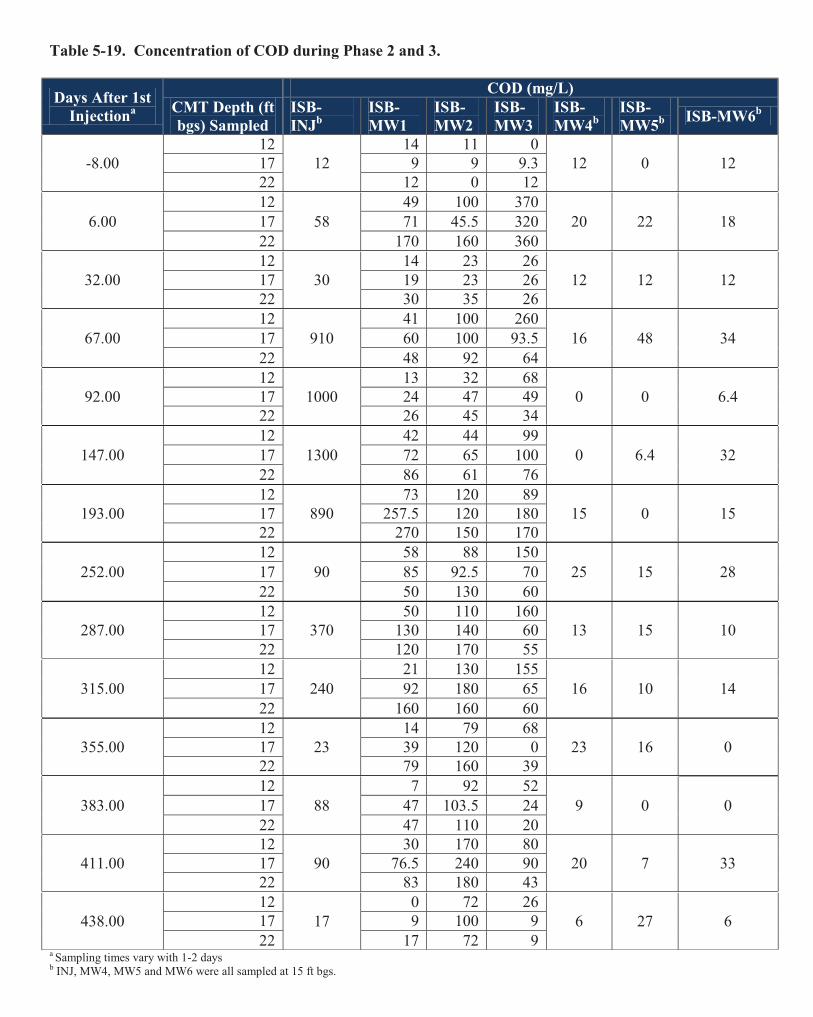
Table 5-19. Concentration of COD during Phase 2 and 3.
Days After 1st Injectiona CMT Depth (ft
bgs) Sampled
COD (mg/L)ISB-INJb
ISB-MW1
ISB-MW2
ISB-MW3
ISB-MW4b
ISB-MW5b ISB-MW6b
-8.0012
1214 11 0
12 0 1217 9 9 9.322 12 0 12
6.0012
5849 100 370
20 22 1817 71 45.5 32022 170 160 360
32.0012
3014 23 26
12 12 1217 19 23 2622 30 35 26
67.0012
91041 100 260
16 48 3417 60 100 93.522 48 92 64
92.0012
100013 32 68
0 0 6.417 24 47 4922 26 45 34
147.0012
130042 44 99
0 6.4 3217 72 65 10022 86 61 76
193.0012
89073 120 89
15 0 1517 257.5 120 18022 270 150 170
252.0012
9058 88 150
25 15 2817 85 92.5 7022 50 130 60
287.0012
37050 110 160
13 15 1017 130 140 6022 120 170 55
315.0012
24021 130 155
16 10 1417 92 180 6522 160 160 60
355.0012
2314 79 68
23 16 017 39 120 022 79 160 39
383.0012
887 92 52
9 0 017 47 103.5 2422 47 110 20
411.0012
9030 170 80
20 7 3317 76.5 240 9022 83 180 43
438.0012
170 72 26
6 27 617 9 100 922 17 72 9
a Sampling times vary with 1-2 daysb INJ, MW4, MW5 and MW6 were all sampled at 15 ft bgs.
189
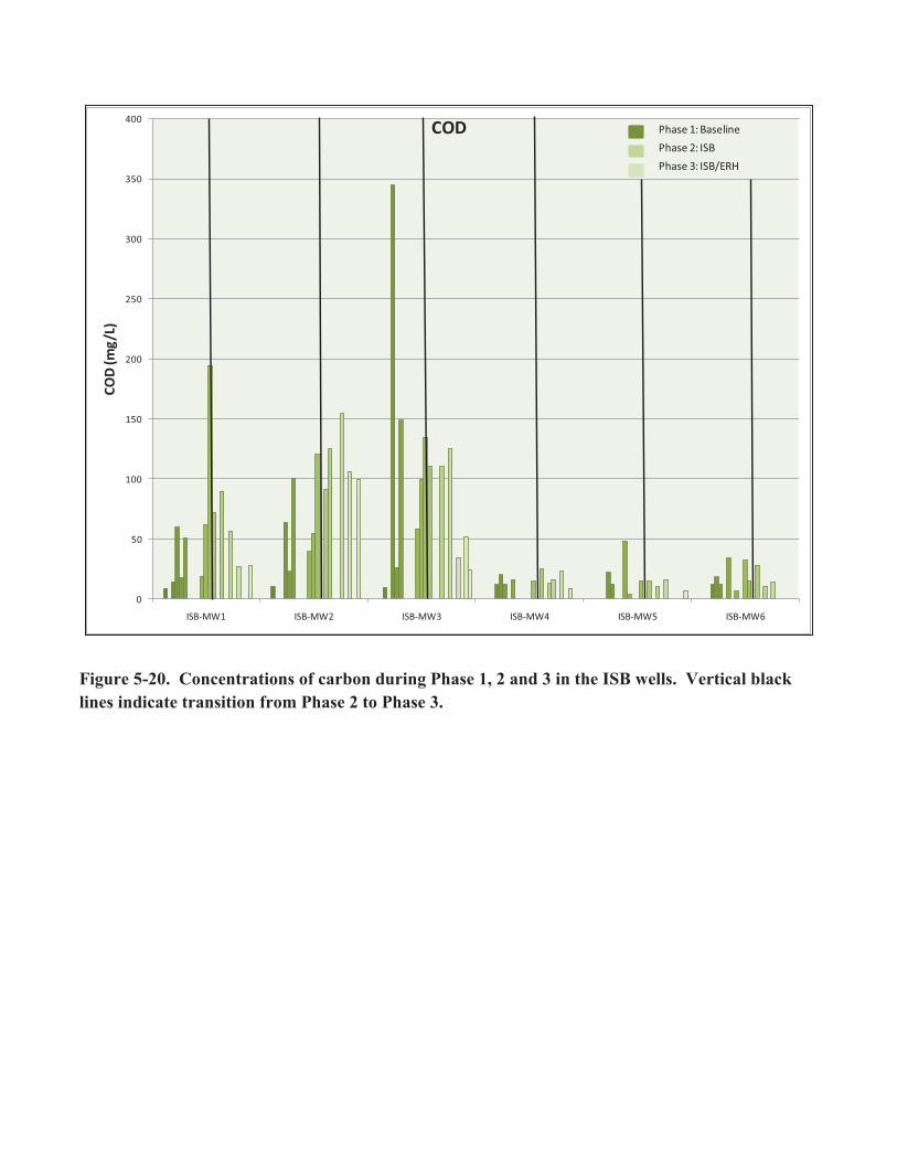
Figure 5-20. Concentrations of carbon during Phase 1, 2 and 3 in the ISB wells. Vertical black lines indicate transition from Phase 2 to Phase 3.
0
50
100
150
200
250
300
350
400
ISB-MW1 ISB-MW2 ISB-MW3 ISB-MW4 ISB-MW5 ISB-MW6
COD
(mg/
L)COD Phase 1: Baseline
Phase 2: ISBPhase 3: ISB/ERH

Section 5 • Test Design
85 ESTCP ER-0719 Final Report
In addition, relatively high concentrations were observed within the ISB test cell (ISB-MW1 through ISB-MW3) approximately 6-20 ft downgradient of ISB-INJ within concentration ranging from approximately 49-370 mg/L. COD concentrations in downgradient MWs ISB-MW4 through –MW6 were slightly greater than baseline. COD concentrations were generally depleted in all of the monitored wells one month post-EOS®11 injection with concentrations ranging from 12-35 mg/L.
Following the EOS®22 injection, measured COD concentrations were sustained between 900-1000 mg/L one and two months post-injection within the ISB-INJ. Elevated levels of COD were also observed 1 month post –EOS®22 injection within the test cell with concentrations ranging from 41-260 mg/L). Two months post-EOS®22, however, concentrations in all monitored wells, except ISB-INJ, were generally depleted with concentrations ranging from 0-68 mg/L). The inability to sustain concentrations of COD for longer than approximately 1 month post-EOS® injections led to the decision to switch the amendment to bicarbonate buffered whey. This was largely due to the necessity to conduct much more frequent injections with EOS® than is cost-effective. For high-frequency injections, bicarbonate-buffered whey is much more cost effective compared to EOS®.
Following Phase 2 injection with whey, COD concentrations were maintained at approximately 42-270 mg/L within the ISB test cell (MW1 through MW-3) one month post-whey 1 and whey 2 injections. Concentrations at downgradient locations ISB-MW4 through-MW6 remained low (0-32 mg/L).
During Phase 3, whey/bicarbonate injections continued and concentrations were initially slightly lower overall (Table 5-19) with values varying from 50-170 mg/L during the first 3 months of operations and continuing to decline to with values ranging from 0-160 the last 3 months of

Section 5 • Test Design
86
ESTCP ER-0719 Final Report
heating within the heated zone. Similarly, concentration declined slightly in the injection well. COD concentrations at downgradient locations ISB-MW4 through-MW6 remained low (0-33 mg/L).
Geochemical Response Chlorinated hydrocarbons serve as electron acceptors in microbially-mediated redox reactions during reductive dechlorination. Therefore, they have to compete with naturally occurring electron acceptors in groundwater. During bioremediation, injection of nutrients in sufficient quantities drives redox conditions from aerobic nitrate reducing iron reducing sulfate reducing methanogenic. For reductive dehalogenation, dechlorination of PCE and TCE to cis-1,2-DCE generally occurs under iron-reducing to sulfate-reducing conditions. Complete dechlorination to ethene typically occurs under sulfate-reducing to methanogenic conditions. Thus, understanding redox conditions provides key insight into the potential for reductive dechlorination to occur at a site. The concentrations of various electron acceptors are discussed below to assess the accurate redox conditions within the ISB test cell. Figure 5-21 illustrates the typical response in redox conditions during progression of the ISB demonstration.
Dissolved Oxygen. DO concentration of less than 0.5 mg/L is considered optimal for dechlorination (data presented in Appendix A). During the baseline sampling event the DO concentrations were observed between 1.8 mg/L to 3 mg/L at all the wells except ISB-MW3 (0.5 mg/L). Immediately following donor injection the DO concentrations decreased and were observed below 0.5 mg/L indicating that the donor injection has successfully created anoxic conditions within and downgradient of the ISB test cell.
Nitrate. Nitrate concentration of less than 1 mg/L is desirable for efficient dechlorination (data presented in BA). During the baseline sampling event the nitrate concentrations were observed near 2 mg/L at all the MWs. Immediately following donor injection the nitrate concentrations decreased to non-detect, which has been sustained throughout Phase 2 and 3 operations. These results indicate that within and downgradient of the ISB test cell, nitrate reduction was occurring following the donor injections.
Ferrous Iron. Ferrous iron is the product of ferric iron reduction. Ferrous iron concentration of greater than 1 mg/L is considered optimal for dechlorination. Figure 5-21 illustrates typical dissolved (ferrous) iron concentrations for the ISB test cell. During the baseline sampling event near zero concentrations of ferrous iron were observed at all the wells except well ISB-MW2 (0.4 mg/L). Increase in ferrous iron concentrations have been observed at all the wells following Phase 2 nutrient injections with concentrations ranging from 2 mg/L to 4 mg/L during August 2009 sampling event. During Phase 3, elevated dissolved iron concentrations were observed within the test cell with concentrations generally above 3 mg/L for all sampling events. The results indicate that iron reducing conditions were developed within and downgradient of the ISB test cell during Phases 2 and 3.
Sulfate. Optimal dechlorination rates are supported by sulfate concentration of less than 1 mg/L. Figure 5-21 illustrates typical sulfate concentrations for the ISB test cell. The sulfate

0
2000
4000
6000
8000
10000
12000
14000
16000
18000
02468
101214161820
Met
hane
(��g/
L)
SO4,
NO
4, D
O, F
e2+ (m
g/L)
Dissolved oxygen Nitrate Sulfate Ferrous Iron Methane
Figure 5-21. Typical progression of redox parameters during Phase 2 and 3.
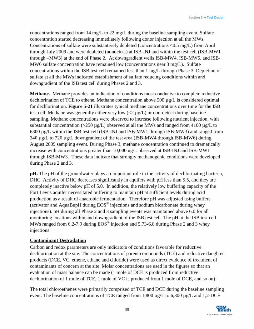
Section 5 • Test Design
88
ESTCP ER-0719 Final Report
concentrations ranged from 14 mg/L to 22 mg/L during the baseline sampling event. Sulfate concentration started decreasing immediately following donor injection at all the MWs. Concentrations of sulfate were substantively depleted (concentrations <0.5 mg/L) from April through July 2009 and were depleted (nondetect) at ISB-INJ and within the test cell (ISB-MW1 through –MW3) at the end of Phase 2. At downgradient wells ISB-MW4, ISB-MW5, and ISB-MW6 sulfate concentration have remained low (concentrations near 3 mg/L). Sulfate concentrations within the ISB test cell remained less than 1 mg/L through Phase 3. Depletion of sulfate at all the MWs indicated establishment of sulfate reducing conditions within and downgradient of the ISB test cell during Phases 2 and 3.
Methane. Methane provides an indication of conditions most conducive to complete reductive dechlorination of TCE to ethene. Methane concentration above 500 µg/L is considered optimal for dechlorination. Figure 5-21 illustrates typical methane concentrations over time for the ISB test cell. Methane was generally either very low (<2 µg/L) or non-detect during baseline sampling. Methane concentrations were observed to increase following nutrient injection, with substantial concentration (>250 µg/L) observed at all the MWs and ranged from 4100 µg/L to 6300 µg/L within the ISB test cell (ISB-INJ and ISB-MW1 through ISB-MW3) and ranged from 340 µg/L to 720 µg/L downgradient of the test area (ISB-MW4 through ISB-MW6) during August 2009 sampling event. During Phase 3, methane concentration continued to dramatically increase with concentrations greater than 10,000 ug/L observed at ISB-INJ and ISB-MW1 through ISB-MW3. These data indicate that strongly methanogenic conditions were developed during Phase 2 and 3.
pH. The pH of the groundwater plays an important role in the activity of dechlorinating bacteria, DHC. Activity of DHC decreases significantly in aquifers with pH less than 5.5, and they are completely inactive below pH of 5.0. In addition, the relatively low buffering capacity of the Fort Lewis aquifer necessitated buffering to maintain pH at sufficient levels during acid production as a result of anaerobic fermentation. Therefore pH was adjusted using buffers (activator and AquaBupH during EOS® injections and sodium bicarbonate during whey injections). pH during all Phase 2 and 3 sampling events was maintained above 6.0 for all monitoring locations within and downgradient of the ISB test cell. The pH at the ISB test cell MWs ranged from 6.2-7.9 during EOS® injection and 5.73-6.8 during Phase 2 and 3 whey injections.
Contaminant Degradation Carbon and redox parameters are only indicators of conditions favorable for reductive dechlorination at the site. The concentrations of parent compounds (TCE) and reductive daughter products (DCE, VC, ethene, ethane and chloride) were used as direct evidence of treatment of contaminants of concern at the site. Molar concentrations are used in the figures so that an evaluation of mass balance can be made (1 mole of DCE is produced from reductive dechlorination of 1 mole of TCE, 1 mole of VC is produced from 1 mole of DCE, and so on).
The total chloroethenes were primarily comprised of TCE and DCE during the baseline sampling event. The baseline concentrations of TCE ranged from 1,800 µg/L to 6,300 µg/L and 1,2-DCE
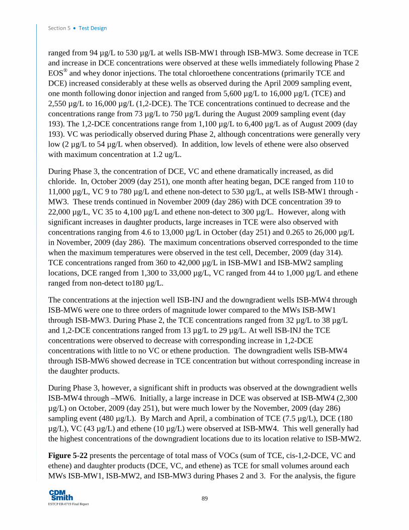
Section 5 • Test Design
89 ESTCP ER-0719 Final Report
ranged from 94 µg/L to 530 µg/L at wells ISB-MW1 through ISB-MW3. Some decrease in TCE and increase in DCE concentrations were observed at these wells immediately following Phase 2 EOS® and whey donor injections. The total chloroethene concentrations (primarily TCE and DCE) increased considerably at these wells as observed during the April 2009 sampling event, one month following donor injection and ranged from 5,600 µg/L to 16,000 µg/L (TCE) and 2,550 µg/L to 16,000 µg/L (1,2-DCE). The TCE concentrations continued to decrease and the concentrations range from 73 µg/L to 750 µg/L during the August 2009 sampling event (day 193). The 1,2-DCE concentrations range from 1,100 µg/L to 6,400 µg/L as of August 2009 (day 193). VC was periodically observed during Phase 2, although concentrations were generally very low (2 µg/L to 54 µg/L when observed). In addition, low levels of ethene were also observed with maximum concentration at 1.2 ug/L.
During Phase 3, the concentration of DCE, VC and ethene dramatically increased, as did chloride. In, October 2009 (day 251), one month after heating began, DCE ranged from 110 to 11,000 µg/L, VC 9 to 780 µg/L and ethene non-detect to 530 µg/L, at wells ISB-MW1 through -MW3. These trends continued in November 2009 (day 286) with DCE concentration 39 to 22,000 µg/L, VC 35 to 4,100 µg/L and ethene non-detect to 300 µg/L. However, along with significant increases in daughter products, large increases in TCE were also observed with concentrations ranging from 4.6 to 13,000 µg/L in October (day 251) and 0.265 to 26,000 µg/L in November, 2009 (day 286). The maximum concentrations observed corresponded to the time when the maximum temperatures were observed in the test cell, December, 2009 (day 314). TCE concentrations ranged from 360 to 42,000 µg/L in ISB-MW1 and ISB-MW2 sampling locations, DCE ranged from 1,300 to 33,000 µg/L, VC ranged from 44 to 1,000 µg/L and ethene ranged from non-detect to180 µg/L.
The concentrations at the injection well ISB-INJ and the downgradient wells ISB-MW4 through ISB-MW6 were one to three orders of magnitude lower compared to the MWs ISB-MW1 through ISB-MW3. During Phase 2, the TCE concentrations ranged from 32 µg/L to 38 µg/L and 1,2-DCE concentrations ranged from 13 µg/L to 29 µg/L. At well ISB-INJ the TCE concentrations were observed to decrease with corresponding increase in 1,2-DCE concentrations with little to no VC or ethene production. The downgradient wells ISB-MW4 through ISB-MW6 showed decrease in TCE concentration but without corresponding increase in the daughter products.
During Phase 3, however, a significant shift in products was observed at the downgradient wells ISB-MW4 through –MW6. Initially, a large increase in DCE was observed at ISB-MW4 (2,300 µg/L) on October, 2009 (day 251), but were much lower by the November, 2009 (day 286) sampling event (480 µg/L). By March and April, a combination of TCE (7.5 µg/L), DCE (180 µg/L), VC (43 µg/L) and ethene (10 µg/L) were observed at ISB-MW4. This well generally had the highest concentrations of the downgradient locations due to its location relative to ISB-MW2.
Figure 5-22 presents the percentage of total mass of VOCs (sum of TCE, cis-1,2-DCE, VC and ethene) and daughter products (DCE, VC, and ethene) as TCE for small volumes around each MWs ISB-MW1, ISB-MW2, and ISB-MW3 during Phases 2 and 3. For the analysis, the figure

�
0
20
40
60
80
100
120
140
0
0.2
0.4
0.6
0.8
1
1.2
1.4
Chlorid
e�(uM)
VOCs�an
d�Ethe
ne�(u
M)
TCE� cis�1,2�DCE� Vinyl�chloride� Ethene� Sum Chloride��
B�
ISB�MW4�
Figure 5-22. Phase 2 and 3 total molar VOC mass in ISB test cell (A) and downgradient concentration at ISB-MW4 (B).
0
5
10
15
20
25
30
35
40
45
0
20
40
60
80
100
120
140
160
180
200
�8 6 32 63 92 147 193 251 286 314 355 384 411
Tempe
rature(C)
VOC�(as�g
�of�TCE
)
Days�After�Injections
cisDCE/VC/ethene�MW1 cis�DCE/VC/ethene�MW2 cisDCE/VC/ethene�MW3
Total�VOC�MW1 Total�VOC�MW2 Total�VOC�MW3
Temperature
A�
120
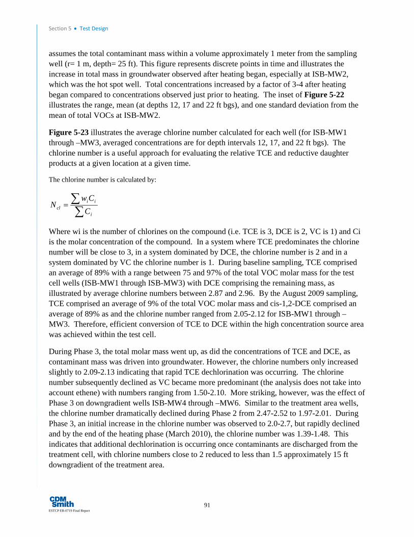
Section 5 • Test Design
91 ESTCP ER-0719 Final Report
assumes the total contaminant mass within a volume approximately 1 meter from the sampling well (r= 1 m, depth= 25 ft). This figure represents discrete points in time and illustrates the increase in total mass in groundwater observed after heating began, especially at ISB-MW2, which was the hot spot well. Total concentrations increased by a factor of 3-4 after heating began compared to concentrations observed just prior to heating. The inset of Figure 5-22 illustrates the range, mean (at depths 12, 17 and 22 ft bgs), and one standard deviation from the mean of total VOCs at ISB-MW2.
Figure 5-23 illustrates the average chlorine number calculated for each well (for ISB-MW1 through –MW3, averaged concentrations are for depth intervals 12, 17, and 22 ft bgs). The chlorine number is a useful approach for evaluating the relative TCE and reductive daughter products at a given location at a given time.
The chlorine number is calculated by:
∑∑=
i
iicl C
CwN
Where wi is the number of chlorines on the compound (i.e. TCE is 3, DCE is 2, VC is 1) and Ci is the molar concentration of the compound. In a system where TCE predominates the chlorine number will be close to 3, in a system dominated by DCE, the chlorine number is 2 and in a system dominated by VC the chlorine number is 1. During baseline sampling, TCE comprised an average of 89% with a range between 75 and 97% of the total VOC molar mass for the test cell wells (ISB-MW1 through ISB-MW3) with DCE comprising the remaining mass, as illustrated by average chlorine numbers between 2.87 and 2.96. By the August 2009 sampling, TCE comprised an average of 9% of the total VOC molar mass and cis-1,2-DCE comprised an average of 89% as and the chlorine number ranged from 2.05-2.12 for ISB-MW1 through –MW3. Therefore, efficient conversion of TCE to DCE within the high concentration source area was achieved within the test cell.
During Phase 3, the total molar mass went up, as did the concentrations of TCE and DCE, as contaminant mass was driven into groundwater. However, the chlorine numbers only increased slightly to 2.09-2.13 indicating that rapid TCE dechlorination was occurring. The chlorine number subsequently declined as VC became more predominant (the analysis does not take into account ethene) with numbers ranging from 1.50-2.10. More striking, however, was the effect of Phase 3 on downgradient wells ISB-MW4 through –MW6. Similar to the treatment area wells, the chlorine number dramatically declined during Phase 2 from 2.47-2.52 to 1.97-2.01. During Phase 3, an initial increase in the chlorine number was observed to 2.0-2.7, but rapidly declined and by the end of the heating phase (March 2010), the chlorine number was 1.39-1.48. This indicates that additional dechlorination is occurring once contaminants are discharged from the treatment cell, with chlorine numbers close to 2 reduced to less than 1.5 approximately 15 ft downgradient of the treatment area.

Figure 5-23. Chlorine numbers calculated for wells ISB-INJ, ISBMW-1 through-MW3 (average of depths 12, 17, and 22 ft bgs) and downgradient wells ISB-MW4 through –MW6 during the demonstration.
1
1.5
2
2.5
3
3.5
Chlo
rine
Num
ber
Days After Injections Began
Chlorine Number
ISB-INJ
ISB-MW1
ISB-MW3
ISB-MW4
ISB-MW5
ISB-MW6
ISB-MW2
Phase 2 Phase 3

Section 5 • Test Design
93 ESTCP ER-0719 Final Report
Mass Flux And Discharge Modeling Groundwater hydraulic and contaminant data were input into the Mining Visualization System (MVS) Version 9.52 software to evaluate mass discharge from the test cell over time during Phase 2, after reducing conditions had been established, and Phase 3. The model utilizes a constant rectilinear grid at a 121x121x35 (X, Y, Z) resolution. Effective porosity was set at 18% and hydraulic conductivity was set to 434 ft/day from 6.5-15 ft bgs, from 464 ft/d from 15-20, and 564 ft/d from 20-25 ft bgs in X, Y direction and half this value in the Z direction (i.e. Kz= ½ [Kx, Ky]).
The seepage velocity module was used to compute a vector groundwater flow field. The module outputs vector data representing X, Y, and Z components. The seepage velocities were calculated from interpolated water levels, hydraulic conductivity and effective porosity in to arrive at a vector seepage velocity (Vx, Vy, Vz) at each node, by taking the gradient of (kriged) head (without any z-exaggeration) and multiplying each component of head gradient by the component of conductivity at that node (based on its material) (Kx, Ky, Kz) and dividing by the Effective Porosity (Ne) for that material.
Vx = dH/dx * Kx / Ne [Equation 1]
Vy = dH/dy * Ky / Ne [Equation 2]
Vz = dH/dz * Kz / Ne [Equation 3]
Head data (dH/dx, dy or dz) in the form of water levels were first kriged in three-dimensional space based on water levels as measured in the well screens corresponding to each sampling event. This data was then processed to create streamlines only for a visual representation.
A formula to evaluate mass flux in three dimensions was input into the software that used the calculated seepage velocity data and kriged analytic concentrations for each date range to calculate the moles/sq ft per-day. The results were a vector-based mass flux calculation at a nodal level throughout the model. At each node, mass flux was calculated using the following formula:
Mf= Vs*Ct* ne
The mass flux nodal calculation (in moles per square foot [sqft] per day [d]) were then integrated over a cross section between the observation wells ISB-MW1 and ISB-2 (approximately 16 ft wide and 18.5 ft deep), which were nearly transect to groundwater flow direction (Figure 5-24), this transect was used to evaluate discharge of contaminants over time during Phases 2 and 3.
Figure 5-24 represents the total molar VOC and degradation daughter product mass flux and discharge during the last three sampling events of Phases 2 and all of Phase 3. These data were used to evaluate the relative change in mass flux and discharge, used to infer treatment rates, as a result of increasing temperatures. The total VOC flux in millimole (mmol) per sqft per d is
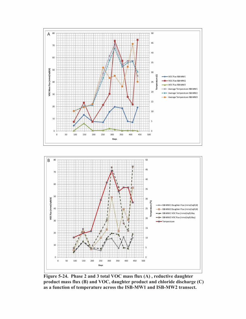
Figure 5-24. Phase 2 and 3 total VOC mass flux (A) , reductive daughter product mass flux (B) and VOC, daughter product and chloride discharge (C) as a function of temperature across the ISB-MW1 and ISB-MW2 transect.
A
B
A

0
5
10
15
20
25
30
35
40
45
50
0
5
10
15
20
25
0 100 200 300 400 500
Tem
pera
ture
( C)
Mas
s Disc
harg
e (m
oles
/day
)
Days from First Injection
Total VOC
Daughter Products (c-DCE, VC, ethene)
TCE
Chloride
Average Temperature ( C)
Figure 5-24 CONT’D. Phase 2 and 3 total VOC mass flux (A) , reductive daughter product mass flux (B) and VOC, daughter product and chloride discharge (C) as a function of temperature across the ISB-MW1 and ISB-MW2 transect.
C

Section 5 • Test Design
96
ESTCP ER-0719 Final Report
illustrated in Figure 5-24A. The mass flux and mass discharge observed at point ISB-MW3 generally declined during the field demonstration. The VOC concentrations at this location were the lowest of the source wells, and it was generally on the upgradient periphery of the source area. In addition, due to preferential heating at this location, the electrode nearest ISB-MW3 was disconnected shortly after the heating system was started, and temperatures were generally 10-15°C lower, on average, compared to ISB-MW2 and ISB-MW1 (Figure 5-24A). Two MWs located downgradient within the source area ISB-MW2 and ISB-MW1 had much higher overall VOC concentrations, especially ISB-MW2. Overall, mass flux increased with temperature, especially at temperatures greater than 35°C (Figure 5-24A and B). The maximum temperature achieved in the test cell was an average of 43°C in December, approximately 314 days after initiation of the demonstration, 90 days after initiation of heating. The VOC mass flux at these locations generally increased during heating with the average increase in mass flux from approximately 8 mmol/sqft/d for both ISB-MW1 and –MW2 during the August (day 193) just before initiating heating to the maximum flux of approximately 74 mmol/sqft/d at ISB-MW2 and 20 mmol/sqft/d at ISB-MW1 in December (day 314) (Figure 5-24A).
The proportion of reductive daughter product mass flux observed is used to determine what percentage of TCE is biologically degraded along the source area ISB-MW1 and -2 transect. Figure 5-24B illustrates the total VOC flux compared to flux of reductive daughter products. During the end of Phase 2, reductive daughter product flux accounted for 81-97% of the total flux, an average of 7.1 and 6.7 mmol/sqft/d at ISB-MW1 and –MW2, during the August (day 193) sampling event before initiating heating on. During the maximum mass flux observed December (day 314), the daughter product flux increased to approximately 15 and 49 mmol/sqft/d average for the three depths at ISB-MW1 and ISB-MW2. This accounted for 41-97% of the total mass flux. This suggests that the rate of reductive dechlorination also increased to reduce the increased mass of contaminants. The mass flux outputs for the nine sampling points within the test cell are presented in Appendix D
The mass flux values calculated using the MVS model were integrated across an area extending from the water table (at 267.5 feet mean sea level [ft msl]) to the bottom of the sample zone (249 ft msl) or approximately 18.5 ft, and extending 16 ft from ISB-MW2 to ISB-MW1. Figure 5-25 illustrates the MVS-modeled temperature profile and VOC, daughter product and chloride mass flux and discharge across the ISB-MW2 and –MW2 transect at three timepoints, one at the end of Phase 2 August (day 193), one a maximum temperature during Phase 3 December (day 314) and one at the end of the heating March (day 411). This figure provides a visual representation of the MVS-modeled analysis and results.
The MVS-modeled discharge from the ISB-MW1 and –MW2 transect prior to heating (n=3 sampling events May, July, and August 09), was 1.8 mole/day corresponding to approximately 240 g of TCE/day (Table 5-20). After heating, the average mass discharge for all 7 post-heating events was 4.8 mole/day corresponding to 633 g/day of TCE, a factor of 2.6 increase in mass discharge. The maximum mass discharge observed during the sampling event corresponding to maximum temperature observed in the test cell (December, day 314) was 7.2 mol/d
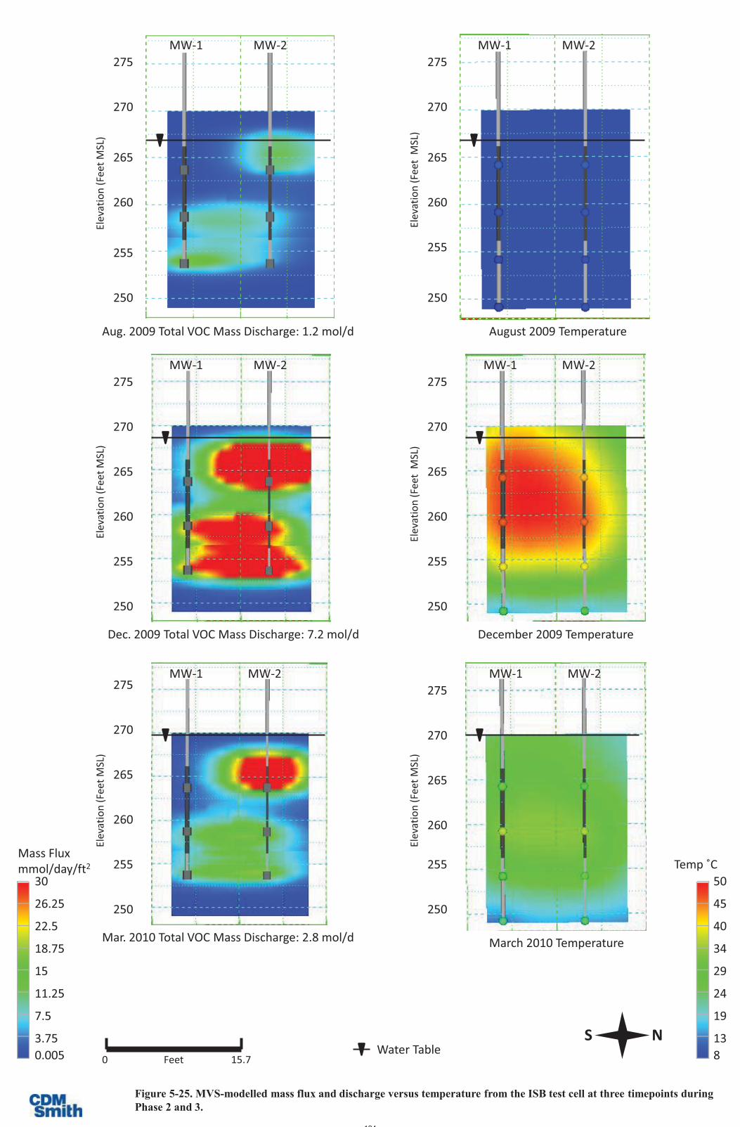
8 13
19
24
29
34
40
45
50 Temp ˚C
N S
Figure 5-25. MVS-modelled mass flux and discharge versus temperature from the ISB test cell at three timepoints during Phase 2 and 3.
0.005 3.75
7.5
11.25
15
18.75
22.5
26.25
30
Mass Flux mmol/day/ft2
0 15.7 Feet
August 2009 Temperature
275
270
265
260
255
250
Elev
atio
n (F
eet
MSL
)
275
270
265
260
255
250
MW-1 MW-2
Elev
atio
n (F
eet M
SL)
Aug. 2009 Total VOC Mass Discharge: 1.2 mol/d
MW-1 MW-2
275
270
265
260
255
250
Elev
atio
n (F
eet
MSL
)
December 2009 Temperature
275
270
265
260
255
250
MW-1 MW-2
Dec. 2009 Total VOC Mass Discharge: 7.2 mol/d
Elev
atio
n (F
eet M
SL)
MW-1 MW-2
Water Table
275
270
265
260
255
250
Elev
atio
n (F
eet M
SL)
March 2010 Temperature
275
270
265
260
255
250
MW-1 MW-2
Elev
atio
n (F
eet M
SL)
Mar. 2010 Total VOC Mass Discharge: 2.8 mol/d
MW-1 MW-2
124

0 13
25
38
50
63
75
88
100
Mass Flux mmol/day/ft2
Aug. 2009 Chloride Mass Discharge: 3.3 mol/d
275
270
265
260
255
250
Elev
atio
n (F
eet
MSL
)
N S
Figure 5-25 (Continued). MVS-modelled mass flux and discharge versus temperature from the ISB test cell at three timepoints during Phase 2 and 3.
275
270
265
260
255
250
Elev
atio
n (F
eet
MSL
)
Dec. 2009 Chloride Mass Discharge: 11.6 mol/d
275
270
265
260
255
250
Elev
atio
n (F
eet M
SL)
Mar. 2010 Chloride Mass Discharge: 12.7 mol/d
275
270
265
260
255
250
Elev
atio
n (F
eet M
SL)
Aug. 2009 Total Daughter Mass Discharge: 1.1 mol/d
275
270
265
260
255
250
Dec. 2009 Total Daughter Mass Discharge: 4.6 mol/d
Elev
atio
n (F
eet M
SL)
275
270
265
260
255
250
Elev
atio
n (F
eet M
SL)
Mar. 2010 Total Daughter Mass Discharge: 2.4 mol/d
0.005 3.75
7.5
11.25
15
18.75
22.5
26.25
30
Mass Flux mmol/day/ft2
MW-1 MW-2
MW-1 MW-2
MW-1 MW-2
0 15.7 Feet Water Table
MW-1 MW-2
MW-1 MW-2
MW-1 MW-2
125

Section 5 • Test Design
99 ESTCP ER-0719 Final Report
Table 5-20. Summary of mass discharge estimates for Phase 2 and 3.
Phase 2 Phase 3
MDout Average mole/day
(n=3) a gTCE/dayb Average mole/day
(n=7) a gTCE/dayb Total VOC 1.8 +/- 1.3 240 4.8 +/- 2.0 633 Products (cis-DCE, VC, ethene) 1.6 +/- 1.3 214 3.6 +/- 1.4 471 Chloride 6.1 +/- 5.7 798 10.7 +/- 3.8 1403 Notes: a Concentrations from all of the monitoring wells were kriged to determine a 3D contaminant plume. Mass discharge was evaluated through a transect 15.8 feet across through ISB-MW1 and -MW2 and 21 feet deep. b g of TCE per day was evaluating by multiplying the molar concentration of Total VOCs or the sum of cis-DCE, VC and ethene by the molecular weight of TCE. TCE dechlorinated based on chloride data was evaluated by taking the chloride molar concentration and subtracting the background chloride (2.5 moles) and then multiplying by the molecular weight of TCE. It was assumed that 1 mole of chloride corresponded to 1 mole of TCE dechlorinated as cis-DCE was the predominant by-product.
corresponding to approximately 943 g/d of TCE, a factor of 3.9 increase in mass discharge. This enhanced mass transfer occurred in the test cell during heating and is primarily attributed to the heating effects (i.e. accelerated dissolution and kinetics). It is assumed that contaminant flux coming into the test cell is negligible since VOC concentrations at ISB-INJ upgradient of the test cell were generally 2-4 orders of magnitude lower than concentration observed at ISB-MW1, -MW2 or -MW-3. Therefore, it was assumed that all of the contaminants were derived from residual source material within the test cell itself.
In addition to total VOCs, mass discharge of daughter products from the test cell was evaluated to determine the biodegradation efficiency within the heated zone. Of the 240 g/day of TCE-equivalent VOC mass discharged from the test cell 214 g/day or 89% was observed as daughter products during Phase 2. This was primarily DCE (89-99% of the molar mass of daughter products DCE, VC and ethene during the August 09 event). During Phase 3, total molar daughter products increased to an average of 471 g/d TCE-equivalent treated, a factor increase of 2.2. Again, DCE was the primary degradation product (13-98%), although significant quantities of VC and ethene were also observed at many locations. The maximum discharge of daughter products occurred during the December (day 314) event, which increased to 607 g/d as TCE, or 64% of the total VOC discharge.
In addition to daughter products, mass discharge using chloride was also evaluated. If applicable, chloride is generally more conservative compared to a molar mass balance using organic degradation by products in groundwater because chloride is conserved in groundwater, while organic VOCs can be degraded (especially VC and ethene/ethane which are very transient within the Landfill 2 shallow aquifer once generated), can partition to the soil, and/or can volatilize to the vadose zone. Biodegradation and volatilization can result in underestimating organic VOC concentrations, and ultimately TCE reactions, when only groundwater data are considered. At Landfill 2, background chloride around the test cell was averaged 70.6

Section 5 • Test Design
100
ESTCP ER-0719 Final Report
micromoles per liter (uM)(average of ISBINJ, ISB-MW4 through –MW6 during baseline, February and March 2009 samplings n=12). This was used as the background and subtracted from the concentrations observed during the active portion of Phase 2 and Phase 3. The adjusted chloride concentrations were input into the MVS model to evaluate TCE dechlorination. Based on an evaluation of chloride flux from the test cell, the average chloride flux during Phase 2 was 6.2 moles/day compared to 15.8 moles/day during heating. This corresponded to an average of 798 g/d of TCE dechlorinated to DCE during Phase 2 and 2078 g/d of TCE dechlorinated to DCE during Phase 3.
Microbial Community Dehalococcoides. The dechlorinating bacteria, DHC, have been found to be very important for achieving complete dechlorination of PCE to ethene in groundwater. Figure 5-26 presents the DNA data over time for the ISB test cell. Only wells ISB-MW1, ISB-MW2, ISB-MW3, and ISB-MW5 were sampled for DNA during the baseline sampling event. The DHC numbers were observed to be > 102 gene copies/L at wells ISB-MW1 through ISB-MW3 and > 103 gene copies/L at well ISB-MW5. Low detection of all three functional genes tceA, bvcA, and vcrA were also observed at some of the wells during the baseline sampling event. During Phase 2, concentrations increased by one to two orders of magnitude to approximately 105 cells/L. Large increases were also observed in functional gene vcrA. Following the onset of heating (days 280 and 385), an additional one to two order of magnitude increase in DHC was observed, along with reductase genes vcrA, bvcA, and tceA.
Methanogens/Sulfate Reducers/Iron Reducers. Other anaerobic members of the microbial community were monitored using molecular tools, including methanogens, sulfate reducers and iron reducers. For methanogens 4 genes were targeted for analysis targeting orders Methanomicrobiales (MMIC), Methanosarcina (MSAR), Methanobacteriales (MBAC), and Methanococcales (MCOC). Of these, only the first three were amplified in samples collected during the demonstration (data presented in Appendix A. Initially, all methanogens were non-detect during the Phase 1, baseline sampling event. By Day 149 and 195 after amendment injections began, increases to 106 to 108 genes/L of groundwater were observed indicating significant growth during Phase 2. During Phase 3, total concentrations of MMIC and MSAR increased to approximately 107 to 109 genes/L of groundwater, indicating an additional one order of magnitude increase. MBAC concentrations, however, were similar or slightly lower during Phase 3 than observed during Phase 2.
For iron-reducing bacteria, average concentrations (ISB-MW1, -MW2 and -MW3) increased from approximately 104 to a maximum of 107 genes/L of groundwater by day 195. However, concentrations declined to an average of 106 by day 288 and to 105 genes/L of groundwater by the end of Phase 3 (day 386).
Molecular analysis of sulfate reducing bacteria, targeting the dsrA gene, was unsuccessful in amplifying this target.

0
5
10
15
20
25
30
35
40
45
1.E+00
1.E+01
1.E+02
1.E+03
1.E+04
1.E+05
1.E+06
1.E+07
1.E+08
-8.00 34 65 149 195 280 385
Tem
pera
ture
( C)
Gene
copi
es/L
gro
undw
ater
Days from 1st injection
vcrA
bvcA
tceA
16S rRNA
Temp
Figure 5-26. Results of molecular DNA Analysis for DHC during Phase 1, 2 and 3 of operations.

Section 5 • Test Design
102
ESTCP ER-0719 Final Report
5.7.1.2 Soil Vapor Monitoring As part of the mass balance approach, an evaluation of heating on increased volatilization of contaminants to the vadose zone and ultimately to the ground surface and potential overlying buildings was conducted. The increase in volatilization was modeled and compared to site-specific shallow soil gas measurements to quantify and confirm contaminant flux to the vadose zone caused by heating.
The model used is a modification of EPA’s Johnson-Ettinger Model (EPA 2004) based on the analytical evaluation of diffusion from groundwater source to ground surface and included a one-dimensional analytical solution for discrete monitoring points. Assumptions used within the model included 1) no advective mechanism for vapor migration and 2) no lateral migration of contaminant by diffusion. Although simplistic, the model correlates well with measured soil gas concentrations at the ground surface and therefore is believed to offer a useful tool to gauge increased flux caused by ERH-enhanced bioremediation.
The model involved analytical derivation of two phenomena: the solubility of the contaminant at various temperatures (i.e., Henry’s Law) and the diffusive flux of contamination from the groundwater source through the vadose zone (i.e., Fick’s First Law of Diffusion). The following site-specific empirical data were used to build and calibrate the model: groundwater temperature, dissolved-phase contaminant concentrations, soil classification, soil porosity, soil temperature, and soil gas contaminant concentrations. The model evaluated flux of TCE, DCE, and VC from groundwater to the ground surface at three discrete points in the project area, MWs MW-1, MW-2, and MW-3, for five discrete sampling events in 2009, January (Baseline), July (Phase 2), August (Phase 2), November (Phase 3), and December (Phase 3).
First, the vapor source concentration, Csource was estimated at the groundwater interface using Henry’s Law and measured contaminant concentration in groundwater. Henry’s constant was determined for each contaminant and adjusted based on measured groundwater temperatures using EPA’s OSWER method (EPA 2001). Second, a derivation of the effective diffusion coefficient, Deff, for the specific lithology of each MW was determined. All three wells were assumed to have two distinct soil horizons. The first was the capillary fringe above the groundwater interface, and the second was the unsaturated zone above the capillary fringe to the ground surface. The diffusion coefficient for each soil horizon was derived using the process detailed in Section 2.3 of EPA 2004 assuming a sandy soil texture to account for both the silt and gravel component of the soil. The diffusivity in air and water of each contaminant was determined at measured soil temperatures, moisture content, and porosity using EPA’s onsite assessment tools (EPA 2011). As noted earlier, Section 2.3 of EPA 2004 provides the details for calculating diffusion coefficients for soil horizons using the Millington and Quirk model and additional soil characteristics provided by Hers (2002). Assumptions or simplifications included in the model were a consistent groundwater level, consistent capillary fringe, and static moisture content of the soil. Deff represents the harmonic mean of the diffusion coefficients for each soil horizon. Also, as noted earlier, the flux model assumed no contaminant concentration at the ground surface, thereby maximizing the modeled flux rate.

Section 5 • Test Design
103 ESTCP ER-0719 Final Report
Third and final, the flux to ground surface was calculated using Fick’s First Law of Diffusion, Csource and the derived Deff. The model was simplified to assume a full concentration gradient through the vadose zone, or in other words, there were no assumed pre-existing soil gas contaminant concentrations which would limit diffusion from the groundwater source. Therefore, the model should be conservative in evaluating risk by overestimating flux.
Lastly, the model was calibrated using flux extrapolated from measured soil gas concentrations at depths of 7 ft bgs and ground surface. The performed calibration was not an independent operation because the empirical flux was derived using the modeled Csource and Deff; however, the calibration is a relative check to verify that the modeled flux at 7 ft bgs and ground surface would yield soil gas concentrations similar to the measured soil gas concentrations.
Modeling Results Table 5-21 presents an example model input for TCE and temperatures profiles for MW-1 during the January, August, and December sampling events, which coincide with the beginning of the project, mid-point at which basic bioremediation ended and ERH-enhanced bioremediation began, and a monitoring point four months into ERH-enhanced bioremediation, with the highest recorded average in situ temperatures.
Table 5-21. TCE and Temperature Profiles for ISB-MW1.
Month TCE GW Conc (µg/L) GW Temp
(°C)
Temp of Capillary Fringe
(°C)
Temp of Unsaturated Zone
(°C) January 14,000 10.1 10 7 August 27 11.6 13 17 December 1,600 45.2 41 18
Using these data as a starting point, the following steps are calculated for each sample event: TCE Csource, TCE Deff for the entire soil column, and finally the TCE flux from groundwater to ground surface. Table 5-22 presents the modeled results. This procedure was repeated for all of the test cell MWs.
Table 5-22. Modeled Results for TCE for ISB-MW1.
Month Csource
(µg/L) Deff
(cm2/sec) Flux
(µg/sec/cm2) January 2,870 1.05e-4 9.87 e-7
August 5.99 1.06 e-4 2.08 e-9
December 1,514 1.16 e-4 5.78 e-7
Figures 5-27, -28, and -29 illustrate the change in flux for TCE, DCE, and VC, respectively, based on bioremediation treatment from during Phase 2 (July and August 2009) and Phase 3 (August to December 2009). The figures also include groundwater temperatures for the modeled flux rates. The figures illustrate how flux varies during the two stages of the study. For the

1.00E-09
1.00E-08
1.00E-07
1.00E-06
1.00E-05
1.00E-04
1.00E-03
Dec-08 Feb-09 Mar-09 May-09 Jul-09 Aug-09 Oct-09 Dec-09 Jan-10
Flux
(μg/
s/cm
2 )
MW-1
MW-2
MW-3
9.9°C
10.1°C
9.5°C
9.2°C
10.3°C
9.2°C
11.8°C
13.0°C
11.6°C
36.1°C
28.2°C
39.9°C
42.4°C
45.2°C
28.0°C 9.2°C = groundwater
Figure 5-27. TCE vapor flux during Phase 1, 2, and 2 for the ISB test cell.

1.00E-08
1.00E-07
1.00E-06
1.00E-05
1.00E-04
Dec-08 Feb-09 Mar-09 May-09 Jul-09 Aug-09 Oct-09 Dec-09 Jan-10
Flux
(μg/
s/cm
2 )
MW-1
MW-2
MW-3
9.9°C
9.5°C
10.1°C
9.2°C
10.3°C
9.5°C
11.8°C
13.0°C
11.6°C
36.1°C
28.2°C
39.9°C
42.4°C
28.0°C
45.2°C
9.2°C = groundwater temperature
Figure 5-28. cis-DCE vapor flux during Phase 1, 2, and 2 for the ISB test cell.

1.00E-10
1.00E-09
1.00E-08
1.00E-07
1.00E-06
1.00E-05
Dec-08 Feb-09 Mar-09 May-09 Jul-09 Aug-09 Oct-09 Dec-09 Jan-10
Flux
(μg/
s/cm
2 )
MW-1
MW-2
MW-3
9.9°C
9.5°C
10.1°C
9.2°C
10.3°C
9.5°C
11.8°C
13.0°C 11.6°C
28.2°C
36.1°C
39.9°C
28.0°C
42.4°C
45.2°C
9.2°C = groundwater temperature
Figure 5-29. VC vapor flux during Phase 1, 2, and 2 for the ISB test cell.

Section 5 • Test Design
107 ESTCP ER-0719 Final Report
January to August timeframe when basic bioremediation was conducted, TCE flux generally declined by two orders of magnitude as reductive dechlorination reduced the mass of TCE, and fluxes of DCE and VC increased by less than an order of magnitude as the mass of daughter compounds increased during reductive dechlorination. During Phase 3, the flux of TCE and DCE increased by approximately two orders of magnitude as increases in system temperature increased dissolution and volatilization of the contaminants. The flux of VC increased by as much as three orders of magnitude for similar reasons as TCE and DCE and also because VC was almost non-existent in the system prior to bioremediation, and therefore reductive dechlorination greatly increased the mass of VC more so than another daughter compound like DCE.
Increases in mass flux to the vadose zone were most dramatic after the onset of heating (November 2009), but generally declined over time. For instance, modeled fluxes for December were slightly less than the modeled fluxes for November even though the system temperatures generally were greater in December. These results indicate dechlorination rates may have increased to a level sufficient to reduce contaminant flux to the vadose zone.
A one-dimensional analytical model was developed to estimate changes in flux caused by diffusion from increased solubility and volatilization of contaminants during ERH-enhanced bioremediation. The model was mostly developed using site-specific data to estimate chemical conditions and physical characteristics at the site, but it also included assumptions and generalizations to minimize the complexity of modeling the capillary fringe and unsaturated zone, especially in relation to deriving diffusion coefficients.
Flux was modeled for TCE, DCE, and VC for five sampling events during 2009: one baseline, two during basic bioremediation efforts, and two during ERH-enhanced bioremediation. The modeled results were expected in that TCE flux decreased during Phase 2 and DCE and VC flux increased due to higher concentration of these compounds in groundwater. During Phase 3, however, TCE, DCE and VC increased by at least two orders of magnitude during ERH-enhanced bioremediation initially during the November sampling event. By the December sampling event, however, it appears that flux beginning to decrease as ERH-enhanced biodegradation rates increased.
The model was calibrated with extrapolated flux measurements derived from analytical concentrations of soil gas samples collected during the sample events. Although about 25% of the extrapolated flux estimates were negative because measured concentrations exceeded Csource, the modeled flux estimates overall correlated very strongly with the extrapolated flux estimates, especially for the flux estimates at the ground surface where many of the uncertainties associated with modeling diffusion through the capillary fringe are muted by the length of the unsaturated zone.
Calibration Of Model Soil gas samples were collected from 7 ft bgs and at ground surface during the same five sampling events: January, July, August, November, and December 2009. These data have been
Section 5 • Test Design
108
ESTCP ER-0719 Final Report
used to evaluate the general accuracy of the modeled flux rates by extrapolating a flux rate based on soil gas contaminant concentrations. As noted previously, the calibration is not an independent evaluation because modeled Csource and Deff must be used to extrapolate flux for the soil gas concentrations; however, if the model is a valid tool then the modeled flux should exhibit some degree of consistency with the extrapolated flux.
For the 7 ft bgs depth, 28 out of the 45 extrapolated flux measurements were realistic in that they were a positive number. The 17 cases involving negative flux measurements occurred because the measured soil gas concentration at 7 ft bgs was greater than the modeled Csource. This result is not unexpected for the 7 foot depth given the following reasons: 1) uncertainty in the soil and water characteristics of the capillary fringe which greatly impedes diffusive migration, 2) depressurization of the capillary fringe, and hence an increase in the diffusion coefficient, was not modeled, 3) potential entrainment of contaminant residual source in the capillary fringe and bottom of unsaturated zone, which was not assumed in the model, and 4) greater dissolved groundwater concentrations could be located near to the discrete MW points, which would increase soil gas concentrations near the MW by lateral diffusion. Regardless of these 17 instances where the extrapolated flux was negative, the data set of paired modeled and extrapolated flux rates yields a strong correlation (r2 = 0.996) as demonstrated in Figure 5-30.
The results of the soil gas samples from the ground surface indicate an even better performance of the model. In this case, only 5 of the 45 extrapolated flux measurements yielded a negative flux measurement. All five instances were for TCE in either July or August 2009 at which point bioremediation had decreased TCE mass in the groundwater, but it is possible that soil gas concentrations in the vadose zone had not reached a steady state with the decreasing mass of contaminants in groundwater. Figure 5-31 shows the strong correlation (r2 = 0.999) for the data set of paired modeled and extrapolated flux rates at the ground surface.
The calibration testing indicates that the one-dimensional analytical model generally performs well for estimating flux to the vadose zone during ERH-enhanced ISB and that the predictability of the model improves with increasing distance from the source.

R² = 0.996
0.00E+00
2.00E-05
4.00E-05
6.00E-05
8.00E-05
1.00E-04
-2.00E-05 -1.00E-19 2.00E-05 4.00E-05 6.00E-05 8.00E-05 1.00E-04
Mod
eled
Flu
x (μ
g/s/
cm2 )
Extrapolated Flux (μg/s/cm2)
Figure 5-30. Model and extrapolated vapor flux at 7 feet bgs in the ISB test cell.

R² = 0.9999
0.00E+00
1.00E-05
2.00E-05
3.00E-05
4.00E-05
5.00E-05
-5.00E-06 5.00E-06 1.50E-05 2.50E-05 3.50E-05 4.50E-05
Mod
eled
Flu
x (μ
g/s/
cm2 )
Extrapolated Flux (μg/s/cm2)
Figure 5-31. Modeled and extrapolated vapor flux at ground surface in the ISB test cell.

Section 5 • Test Design
111 ESTCP ER-0719 Final Report
Soil Monitoring Soil concentrations of TCE, DCE, and VC were measured during Phase 1, Baseline, following Phase 2 ambient treatment, and following Phase 3 heated treatment. Soil samples were generally collected within the borehole (Baseline) or within one foot of ISB-MW1, -MW2 and –MW3. Figure 5-32 illustrates results of the Baseline post-Phase 2 and post-Phase 3 soil monitoring. DCE and VC soil concentrations were much lower than the TCE concentrations and are presented only in Appendix E. High concentration of TCE were observed at all monitoring locations, but were generally highest at ISB-MW2 during baseline sampling (5.1-130 mg/kg). Generally soil concentrations decreased following Phase 2 with an average 27% reduction in soil concentrations (n=3). Following Phase 3, average soil concentrations again decreased at ISB-MW1 and ISB-MW2, but dramatically increased in ISB-MW3, indicating that a significant source was still present in this well after Phase 3. However, generally temperatures were much lower at this location than at ISB-MW1 and ISB-MW2 because the electrode nearest this well was turned off shortly after startup because of preferential heating.
Three soil samples were collected from each soil boring and the average concentration was 48.5 mg/kg during baseline (range 4.9-130 mg/kg), 60.0 mg/kg following Phase 2 (range 0.36-220 mg/kg) and 17.5 mg/kg following Phase 3 (range 0.29-100 mg/kg) for an average reduction of 64% compared to baseline and 70% compared to Phase 2 (see Appendix A). However the variability in concentration results, and the high uncertainty in the total mass present within the test cell, limits the ability to interpret the soil results. These data generally support that treatment of TCE in soil was occurring during the test.
5.7.2 ZVI Injection Results Details of the ZVI injection are described by Truex et al. (2010) and summarized below. A tracer test was conducted prior to ZVI injection to evaluate the subsurface flow system and finalize the injection parameters. Table 5-23 shows the comparison of observed tracer breakthrough and the calculated arrival time based on a radial flow assumption and an effective porosity estimate of 0.18. Tracer reached full injected concentration at all wells except ZVI-MW2 (80%), ZVI-MW3 (75%), ZVI-MW6 (85%), and the upgradient well ZVI-MW9 (25%). Tracer arrival at different MWs indicated several preferential pathways from the injection point with the most significant to wells ZVI-MW6 and ZVI-MW8 as indicated by substantially shorter actual arrival times compared to calculated estimates. Overall, however, tracer arrival to the other six MWs was consistent with calculated estimates, indicating that the radial flow assumption was appropriate. Tracer elution evaluation resulted in an estimated average groundwater linear velocity of 16 m/d with a standard deviation of 6.5 m/d. Thus, prior to injection, there was a relatively high groundwater velocity across the test site.
Table 5-24 summarizes the ZVI injection parameters. During injection of the ZVI solution, pressures at the injection well and MWs were higher than observed during the tracer test as expected due to the higher viscosity of the injection solution (Figure 5-33). However, the pressure did not become a limiting factor for injection at the target flow rate. These figures show moderate pressure at the injection well (~1.5 m of head with the SlurryPro™ compared to 0.75 m

Section 5 • Test Design
112
ESTCP ER-0719 Final Report
Table 5-23. Summary of tracer arrival and ZVI distribution results.
Well
Radial Location from Injection Well
(m)
Measured Tracer
Breakthrough (h)1
Calculated Tracer
Breakthrough (h)
Comparison of Measured
to Calculated
Arrival
Average ZVI Concentration
During Injection (% of injection concentration)
MW1 1.22 0.13 0.28 early 26 MW2 2.10 0.87 0.84 OK 1 MW3 2.07 0.75 0.82 OK 1.5 MW4 1.04 0.15 0.20 OK 17 MW5 2.23 0.70 0.94 OK 5 MW6 2.04 0.20 0.79 very early 14 MW7 2.07 0.50 0.82 OK 8 MW8 4.05 0.67 3.12 very early 2.6 MW9 4.27 >2.5 3.46 OK None
abased on time to reach 50% of injected concentration using down-hole bromide probe data.
Table 5-24. Summary of ZVI injection parameters.
Item Value
Water injection rate(average) 20.5 gpm SlurryPro™ injection rate(average) 2.2 gpm Surfactant injection rate (average) 76 mL/min Total solution injection rate (average) 22.7 gpm Total injection solution volume 13,660 L SlurryPro™ stock solution injection volume 1300 L Injected ZVI mass 187 kg SlurryPro™ concentration (average) 0.019 wt% Surfactant concentration (average) 0.0008 wt% ZVI concentration in injection solution 1.36 wt% Injection duration 158 min
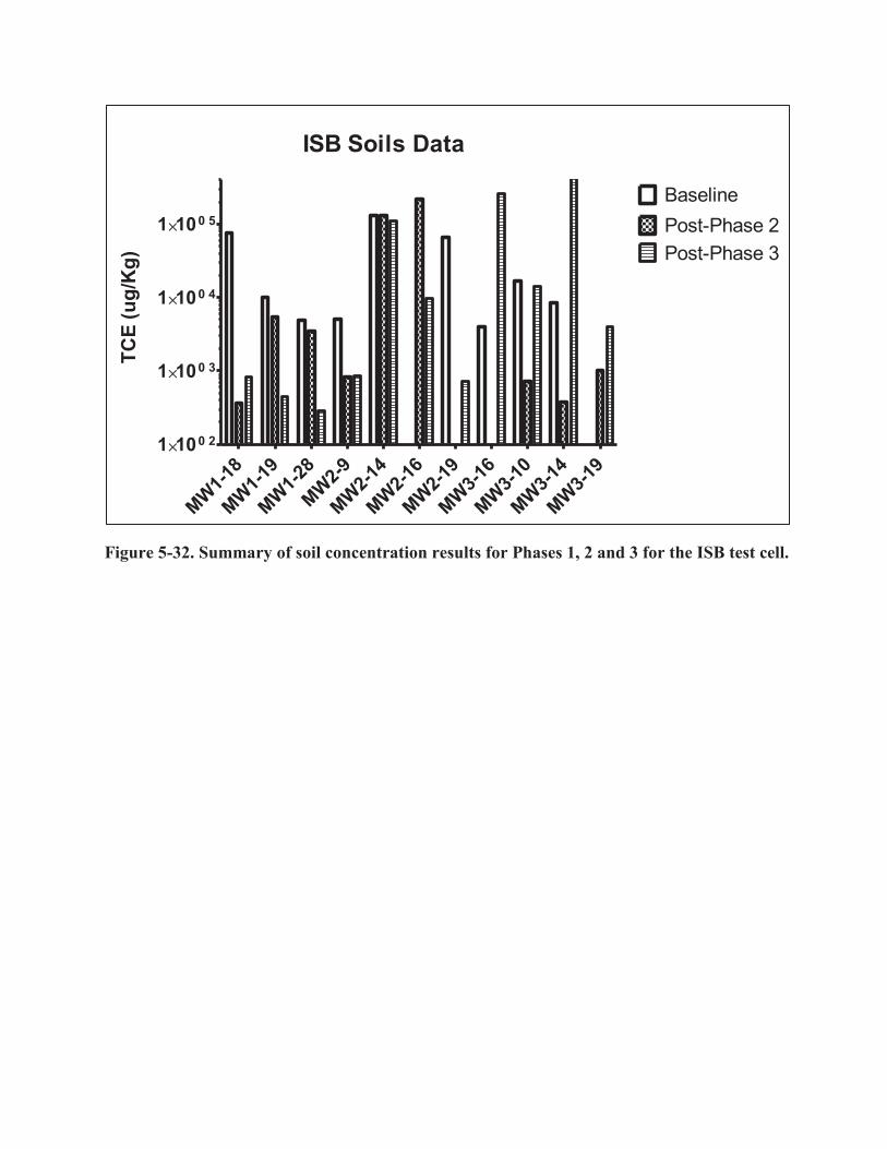
Figure 5-32. Summary of soil concentration results for Phases 1, 2 and 3 for the ISB test cell.
ISB Soils Data
MW1-18
MW1-19
MW1-28
MW2-9
MW2-14
MW2-16
MW2-19
MW3-16
MW3-10
MW3-14
MW3-19
1�100 2
1�100 3
1�100 4
1�100 5
BaselinePost-Phase 2Post-Phase 3
TCE
(ug/
Kg)
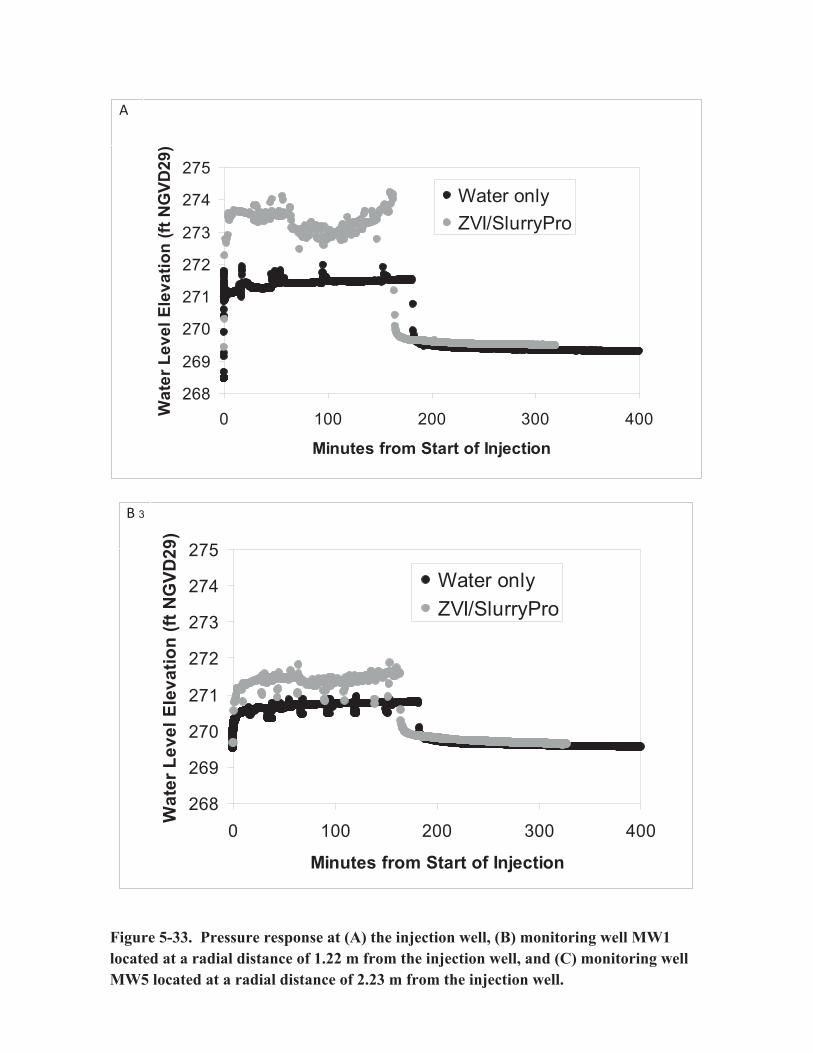
268
269
270
271
272
273
274
275
0 100 200 300 400
Minutes from Start of Injection
Wat
er L
evel
Ele
vatio
n (ft
NG
VD29
)
Water onlyZVI/SlurryPro
268
269
270
271
272
273
274
275
0 100 200 300 400
Minutes from Start of Injection
Wat
er L
evel
Ele
vatio
n (ft
NG
VD29
)
Water onlyZVI/SlurryPro
Figure 5-33. Pressure response at (A) the injection well, (B) monitoring well MW1 located at a radial distance of 1.22 m from the injection well, and (C) monitoring wellMW5 located at a radial distance of 2.23 m from the injection well.
A�
B�3
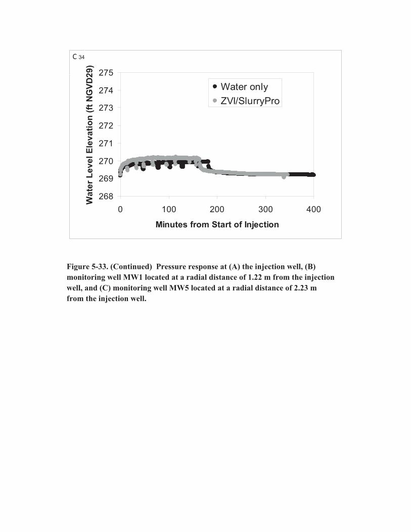
268
269
270
271
272
273
274
275
0 100 200 300 400
Minutes from Start of Injection
Wat
er L
evel
Ele
vatio
n (ft
NG
VD29
)Water onlyZVI/SlurryPro
Figure 5-33. (Continued) Pressure response at (A) the injection well, (B) monitoring well MW1 located at a radial distance of 1.22 m from the injection well, and (C) monitoring well MW5 located at a radial distance of 2.23 m from the injection well.
C�34
Section 5 • Test Design
116
ESTCP ER-0719 Final Report
of head for water injection) and then pressure decreasing with radial distance from the injection well as would be expected with development of a water table mound around the injection point. These pressures suggest normal groundwater flow with no fracturing of the formation.
Table 5-23 shows the ZVI concentration in the MWs as a function of radial distance from the injection well. Decreasing concentration of ZVI with radial distance from the injection well was observed, consistent with the occurrence of some filtration and gravitational settling of ZVI during injection (Oostrom et al. 2007). These results represent measurement of ZVI particles that reached each MW and could be retrieved in the sampling system. The correlation of these data to actual ZVI concentration in the aquifer at these locations is not known. As an additional indication of ZVI distribution, the groundwater chemistry and dechlorination reactions at each monitoring location showed indications of the reductive processes expected with ZVI as discussed in the next section.
5.7.3 Phase 2 and 3: ZVI Analysis of the ZVI treatment results is presented in Truex et al. (2010 and 2011) and summarized below. Data were collected periodically for 345 days after ZVI injection, with the highest data density during the first 150 days. Seasonal water table variation occurred over this test timeframe and the water level decreased such that the test cell screens were below 90% saturated after day 121 with increasing water levels starting around day 184 (Figure 5-34). For this reason, the mass-discharge analysis presented in Section 6 focused on the first 120 days of treatment, 60 days under ambient conditions (Phase 2), and 60 days of heated treatment (Phase 3). The data presentation below provides data for the full duration of the test. However, data past day 121 should be considered in light of the water table variations. Additionally, most of the data analysis focuses on data from the injection well and MWs other than ZVI-MW3. Well ZVI-MW3 was screened in the top 0.6 m of the aquifer and due to the water level variations, having a well screen interval different from other test well, and the proximity of ZVI-MW3 to ZVI-MW2, ZVI-MW3 was not included in most of the data analyses.
Groundwater Monitoring Constituents in groundwater were monitored over time in the ZVI test cell to evaluate the geochemical conditions and the contaminant and dechlorination product concentrations as part of evaluating the ZVI treatment process and the impact of elevated temperature.
Geochemical Response ZVI reactions in groundwater cause a decreased oxidation-reduction potential (ORP) and an increase in pH. The ORP substantially decreased in the test cell upon addition of ZVI and remained low, generally between -100 and -200 mV for the first 150 days of the test, spanning both ambient temperature and elevated temperature conditions (Figure 5-35). The ORP is not a direct measure of dechlorination reactions, but provides an indication that the ZVI was active in chemically reducing the groundwater system over time. When the ORP increased again toward starting ORP conditions it is an indication of the ZVI losing its ability to maintain chemically reducing conditions either through being expended or passivated to an extent that rate of reductive ZVI processes were slower than the rate of oxidizing species into the monitored

Figure 5-34. Water level variation during the field test.
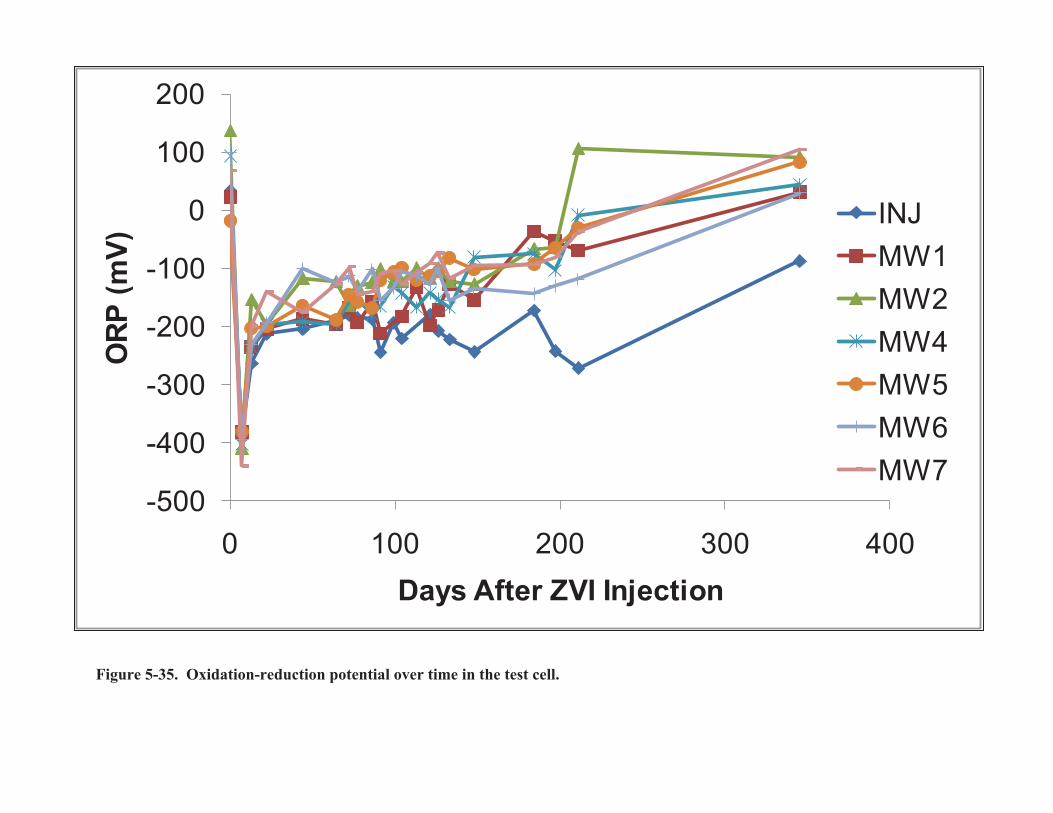
Figure 5-35. Oxidation-reduction potential over time in the test cell.
-500
-400
-300
-200
-100
0
100
200
0 100 200 300 400
ORP
(m
V)
Days After ZVI Injection
INJMW1MW2MW4MW5MW6MW7

Section 5 • Test Design
119 ESTCP ER-0719 Final Report
interval. The low ORP conditions were maintained longest at the injection well were the highest concentration of ZVI was present in the aquifer. Changes in pH (increased due to ZVI reactions with water) showed similar trends in terms of the timeframe of ZVI reactions at the monitoring locations (Figure 5-36).
Contaminant And Dechlorination Product Concentrations The concentrations of TCE (target contaminant) and dechlorination products in the groundwater are the central data need to evaluate treatment over time because the reactions occur in the aqueous phase and collecting and measuring concentrations in groundwater is a robust process. Soil contaminant data are important, but do not provide significant temporal information. Vapor data is important because TCE and its dechlorination products are volatile. However, vapor data can be impacted by interferences in the unsaturated zone where samples are collected (see discussion in next section) and data represent concentrations after transport out of the groundwater and potentially through zones of further degradation processes (e.g., oxidation reactions not present in the groundwater).
The TCE concentration over time is expected to be impacted by dissolution from sediment-associated or DNAPL TCE, dechlorination reactions, and volatilization. Likewise, dechlorination products are impacted by these same processes, although dissolution is expected to be minimal, and potentially by sorption. However, the sorption of the TCE dechlorination products is expected to be low at the test site (Truex et al. 2006). Evaluation of these processes is described in Section 6 using a mass-discharge approach based on the groundwater data presented here. While most of the results interpretation requires a mass-discharge analysis, some general conclusions about contaminant dechlorination can be drawn directly from the contaminant data and are presented below.
The temporal variation in TCE and dechlorination concentrations in the groundwater at each monitoring location are shown in Figures 5-37 through 5-46. At all interior test cell wells, dechlorination daughter products appeared within one week of ZVI injection and showed primarily dechlorination products present by 44 days and continuing through about 120 days after injection. The total organic dechlorination products show a sharp increase during the first 60 days of heating, days 60 – 120 after injection, and then begin to decline. The dominant organic dechlorination daughter products observed were cis-1,2-DCE, ethene, and ethane, indicative of both beta elimination and reductive dechlorination mechanisms. The increases in cis-1,2-DCE concentrations suggest that incomplete biological dechlorination of TCE to cis-1,2-DCE was stimulated rapidly, potentially induced by hydrogen produced by the ZVI. In the absence of VC concentration increases (less than 0.2 uM at all wells within the test cell during the test), the complete biological reductive dechlorination pathway is unlikely and the ethene and ethane concentration increases suggest that beta elimination dechlorination reactions catalyzed by the ZVI were occurring. Acetylene is a transient product of the abiotic reactions and was observed at concentrations ranging up to 0.4 uM at the injection well and wells ZVI-MW3 through -MW7 ranging up to 1.2 uM. Note that dechlorination products were observed in ZVI-MW3 even though this well was screened within a till feature at the top of the aquifer. Data after

5
5.5
6
6.5
7
7.5
8
8.5
9
9.5
0 100 200 300 400
pH
Days from ZVI Injection
INJMW1MW2MW4MW5MW6MW7MW8MW9
�
5
5.5
6
6.5
7
7.5
8
8.5
9
9.5
0 50 100 150
pH
Days from ZVI Injection
INJMW1MW2MW4MW5MW6MW7MW8MW9
�
Figure 5-36. Measured pH response during ZVI demonstration (A) and for first 150 days (B).
A�
B�37

Figure 5-37. Groundwater concentrations at well INJ. (B) graph presents groundwater constituents at a refined scale to show details.
A
B

Figure 5-38. Groundwater concentrations at well MW1. (B) graph presents groundwater constituents at a refined scale to show details.
A
B

Figure 5-39. Groundwater concentrations at well MW2. (B) graph presents groundwater constituents at a refined scale to show details.
B
A
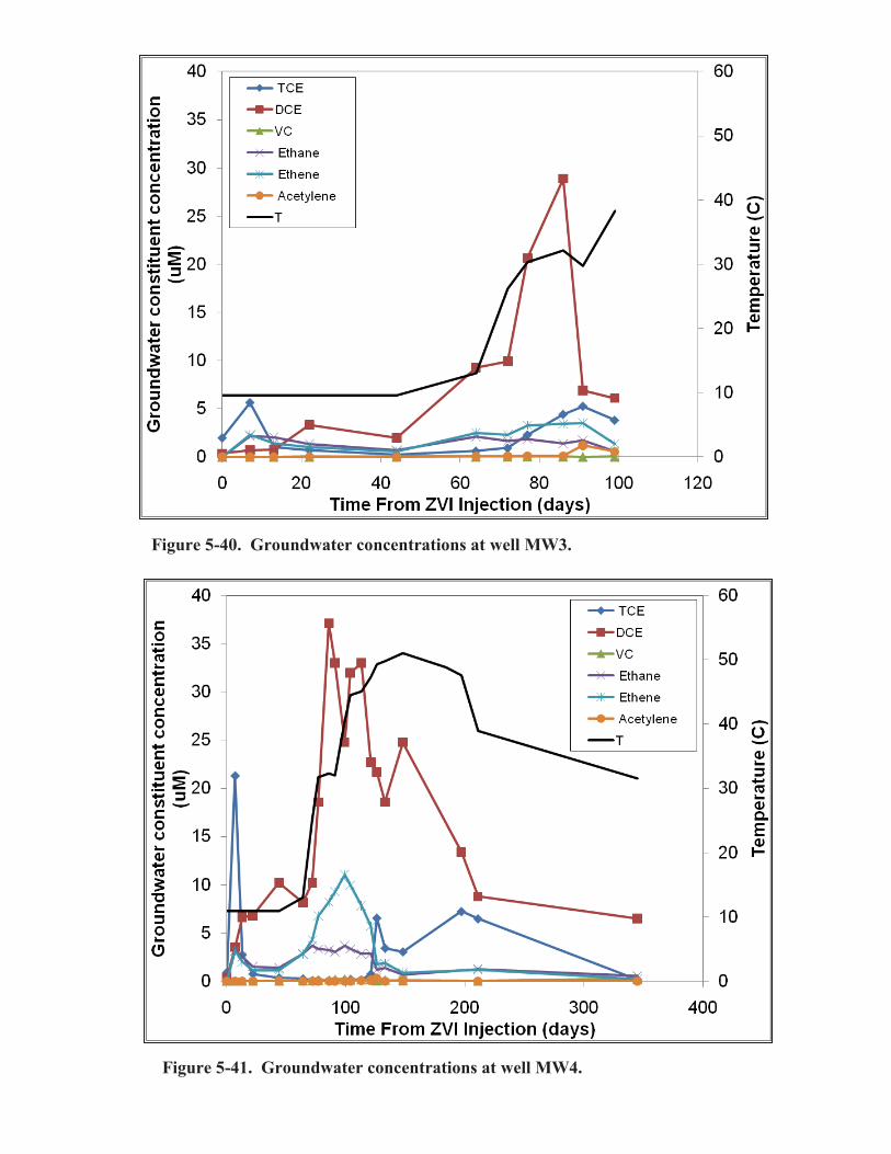
Figure 5-40. Groundwater concentrations at well MW3.
Figure 5-41. Groundwater concentrations at well MW4.

Figure 5-42. Groundwater concentrations at well MW5.
Figure 5-43. Groundwater concentrations at well MW6.

Figure 5-44. Groundwater concentrations at well MW7. (B) graph presents groundwater constituents at a refined scale to show details.
B
A
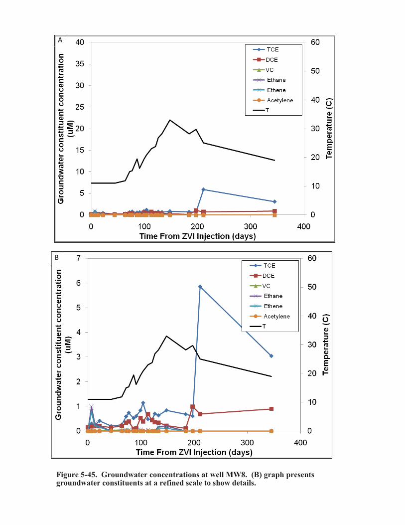
Figure 5-45. Groundwater concentrations at well MW8. (B) graph presents groundwater constituents at a refined scale to show details.
B
A
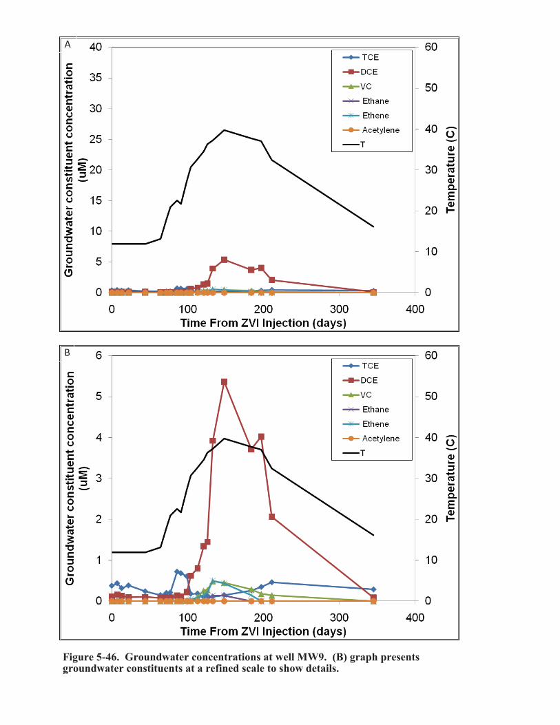
Figure 5-46. Groundwater concentrations at well MW9. (B) graph presents groundwater constituents at a refined scale to show details.
B
A

Section 5 • Test Design
129 ESTCP ER-0719 Final Report
day 100 are not shown for ZVI-MW3 due to water level decreases significantly impacting the screen saturation level.
Additionally, at all of these wells except for the injection well, the total molar VOC concentration increased significantly within one week, including (with the exception of the injection well) an increase in TCE concentration. This apparent increase in molar concentrations suggests that a significant amount of mass transfer may have occurred from the NAPL and/or sorbed phases to the aqueous phase as a result of the ZVI solution injection. Radial displacement of the high pre-injection TCE concentrations near the injection well, TCE desorption, and reaction with ZVI are potential explanations for the increased total VOC concentration (Truex et al. 2010).
The total molar VOC concentration in the groundwater also increased significantly over the first 60 days of Phase 3 heating. Increases in dechlorination daughter products by a factor of about three without increases in TCE mass in the groundwater during initial heating suggest that heating enhanced dechlorination of sediment- or NAPL-associated TCE. The decline in daughter products after about 120 days and the subsequent rise in ORP by day 200 at most locations other than the injection well suggest that the reactivity of the injected ZVI had declined by this time or a decreased mass and therefore availability of TCE within the test cell (see also Truex et al. 2011). TCE groundwater rose at locations other than the injection well after about day 100, suggesting a decline in ZVI reactivity compared to the enhanced dissolution from the elevated temperature conditions.
A transient dechlorination response was observed at well ZVI-MW8, which only received a relatively small dose of ZVI. At ZVI-MW8, only limited dechlorination was observed and by day 44 the water chemistry had nearly returned to pre-injection conditions. The TCE concentration at ZVI-MW8 rose after day 184, but this effect may be related to water level variation during this time. TCE concentrations over time were not significantly impacted for well ZVI-MW9, which did not receive ZVI, until later in the test (after day 100) when the temperature at ZVI-MW9 increased to above 30oC and data show evidence of reductive dechlorination processes occurring. Potentially, biological reactions coupled to organic matter in the sediment were the cause of this dechlorination.
General conclusions can be inferred from the groundwater data. For instance, increases in dechlorination products and decreases in TCE concentration with an overall increase in the total VOC concentration indicate that sediment- or NAPL-associated TCE was being treated and that the ZVI reaction transformed TCE at least as quickly as it was being released from the sediment, even under elevated temperature conditions. Because the groundwater TCE concentrations were maintained low during both Phase 2 and 3 treatment, the driving force for volatilization was low. The groundwater data also indicate that the ZVI induced both reductive dechlorination and beta elimination reactions. The relative rates for these reactions, including an analysis of how temperature impacted these rates is presented in Section 6. As an overall indication of treatment, Table 5-25 shows the TCE and dechlorination concentrations in the groundwater before ZVI injection and at the end of the test. Treatment during the full Phase 2 and 3 duration of the ZVI

Section 5 • Test Design
130
ESTCP ER-0719 Final Report
test resulted in a decrease in groundwater TCE concentration. Except for DCE, final groundwater concentrations of organic dechlorination products were 1 to 2 orders of magnitude higher at the end of treatment. Table 5-25 also shows that initial TCE concentrations were much higher inside compared to outside the test cell, indicating that the test was conducted in a contaminant source zone.
Table 5-25. Average groundwater concentration of TCE and dechlorination products.
TCE (ug/L)
DCE (ug/L)
VC (ug/L)
Ethane (ug/L)
Ethane (ug/L)
Test cell (INJ, MW1, MW2, MW4, MW5, MW6, MW7) Start 3794 672 1 3 5
Finish 93 605 32 171 176 Outside (MW9)
Start 49 17 0 0 0 Finish 37 64 0 0 0
Soil Vapor Monitoring Concentrations of TCE, DCE, VC, ethene, ethane, and acetylene were measured in soil gas samples collected from the unsaturated filter pack sand above the well screen intervals in ZVI-MW2 through –MW7. However, as discussed in Truex et al. (2011), soil gas data were not used in the analysis because pre-test vapor-phase TCE and DCE concentrations were an average of 69 and 15 times higher, respectively, in these vapor samples than vapor concentrations calculated based on the measured groundwater concentration and equilibrium partitioning by Henry’s Law. These data indicated the presence of significant vadose zone contamination above the test cell that would be an interference in directly measuring volatilization of contaminants from the groundwater. In addition to this initial interference for data interpretation, heating during Phase 3 was expected to impact this vadose zone source through enhanced volatilization, but quantification of this heating impact on soil gas concentrations is difficult and impose additional problems for use of the soil gas data to quantify volatilization from the groundwater. For these reasons, the soil gas data were not used in the mass-discharge analysis presented in Section 6. The soil gas data are presented in Appendix E, but not used further.
Soil Monitoring Soil concentrations of TCE, DCE, and VC were measured before ZVI treatment, at the end of Phase 2 ambient treatment, and at the end of the test after Phase 3 heated treatment. Figure 5-47 shows the TCE soil concentrations. DCE and VC soil concentrations were much lower than the TCE concentrations and are presented only in Appendix E. Soil TCE concentrations at the injection well averaged over 100 mg/kg compared to average concentrations of about 2.5 and 1.5 mg/kg at ZVI-MW1 and -MW2, respectively. Moderate decreases in average soil TCE concentrations were observed at ZVI-MW1 and ZVI-MW2 at the end of Phase 2, ambient
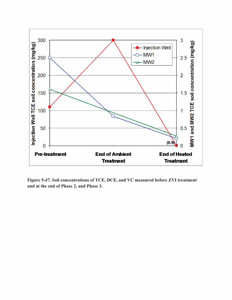
Figure 5-47. Soil concentrations of TCE, DCE, and VC measured before ZVI treatment and at the end of Phase 2, and Phase 3.

Section 5 • Test Design
132
ESTCP ER-0719 Final Report
temperature treatment. Conversely, the average soil TCE concentration remained high with an average of about 300 mg/kg. By the end of the test, soil TCE concentrations were low at all locations dropping to below 1 mg/kg at the injection well. These data suggest that significant treatment of TCE contaminant mass occurred during the test. Other test data suggest that substantial TCE mass reduction occurred by day 120 of the treatment. The amount of mass reduction due to volatilization rather than reaction is difficult to quantify due to the lower data density after day 150. However, in all of these data, the TCE groundwater concentrations were lower than the concentrations of dechlorination products, suggesting that volatilization of TCE was low compared to dissolution and reaction.
Microbial Community Molecular probe data were collected to evaluate the role of microbial reductive dechlorination during the test, in particular with respect to dechlorination DCE to ethane. These data are useful in helping evaluate whether the ethene and ethane observed can be attributed to beta elimination or to microbial reductive dechlorination. Microbial reductive dechlorination is a possible mechanism for production of ethane/ethane during the test, though unlikely due to low observed VC concentrations. Molecular DNA data targeting Dehalococcoides, the bacteria that converts DCE to ethene, remained at low levels during the test, generally below the threshold concentration of 106 gene copy L-1 to observe significant complete biotic dechlorination in JBLM groundwater (Macbeth and Sorenson 2011), confirming biotic DCE degradation was limited (Figure 5-48).
5.7.4 Phase 3: Low-Energy ERH Power and Energy During Phase-3 of operations energy input for the ZVI and ISB test cells were 60,038 kWh and 33,330kWh respectively; totaling 93,368 kWh for the entire project. Total energy input for the entire project was less than the design target of 113,00kWh due to lower than expected heat loss from each test cell. Initial power application to the ZVI test cell was started on June 17, 2009 with initial power application to the ISB test cell starting on September 26, 2009; power application was ceased to both treatment regions on March 22, 2010. Figures 5-49 and Figure 5-50 summarize the total cumulative energy input to both the ZVI and ISB test cells.
Unlike traditional ERH operations where power is consistently applied until the project objectives are met, low temperature heating requires an initial power application to bring the treatment volume to the desired temperature range and then power application is reduced either through cycling power application on and off or by reducing the direct power being applied from the PCU.
During initial heat up of the ZVI test cell daily power application rates averaged 30kW with weekly energy application peaking at 4,333kWh during week three of operations. After initial heat up, daily power application rates averaged 20-25kW to maintain temperatures within the ZVI test cell. Prior to complete removal of power application to both test cells at the end of Phase 3 operations, power was reapplied to the ZVI test cell at an increased rate the week of February 8, 2010 to bring the test cell back up to the desired temperature range. Although Phase3
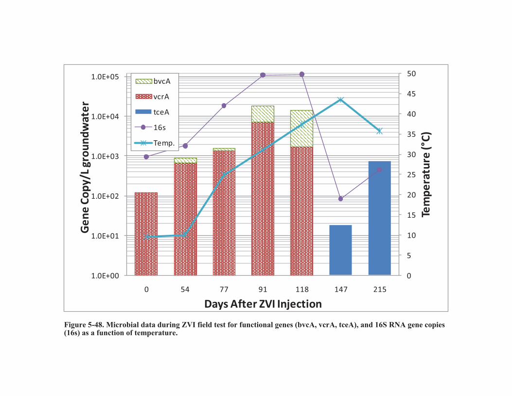
0
5
10
15
20
25
30
35
40
45
50
1.0E+00
1.0E+01
1.0E+02
1.0E+03
1.0E+04
1.0E+05
0 54 77 91 118 147 215
Tem
pera
ture
(°C)
Gene
Cop
y/L g
roun
dwat
er
Days After ZVI Injection
bvcA
vcrA
tceA
16s
Temp.
Figure 5-48. Microbial data during ZVI field test for functional genes (bvcA, vcrA, tceA), and 16S RNA gene copies (16s) as a function of temperature.

Figure 5-49. Cumulative Energy Applied to the ZVI and ISB Test Cells
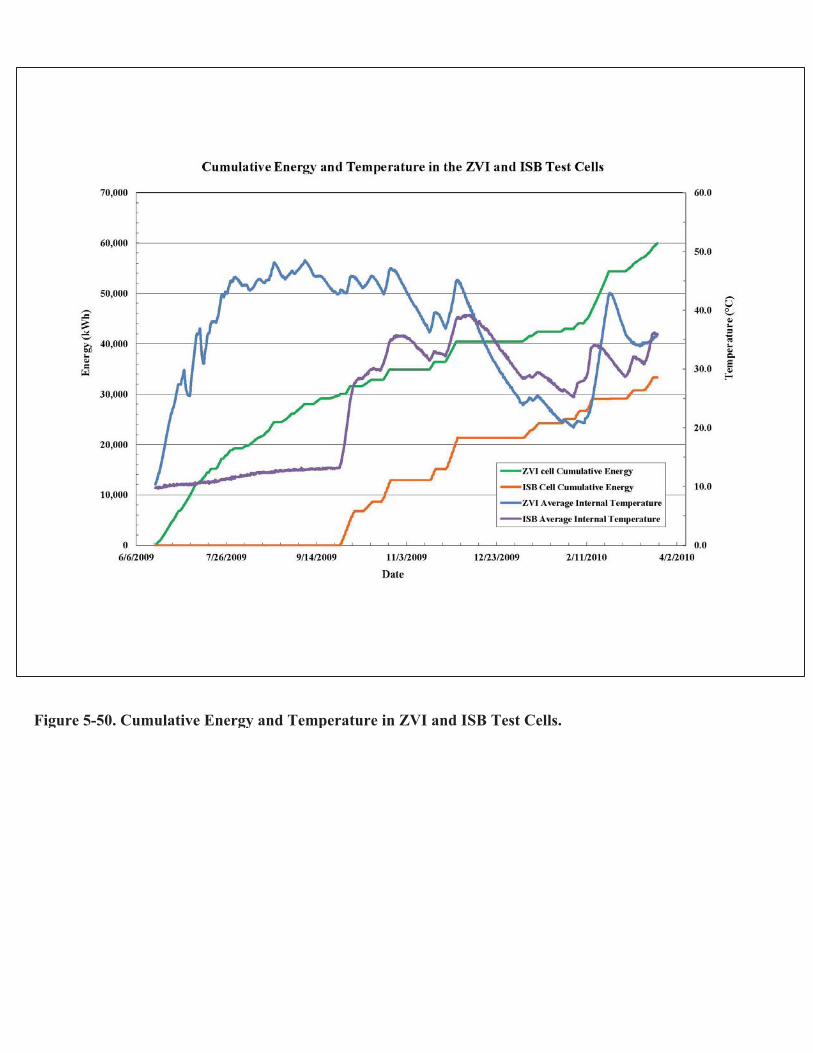
Figure 5-50. Cumulative Energy and Temperature in ZVI and ISB Test Cells.

Section 5 • Test Design
136
ESTCP ER-0719 Final Report
operations were complete for the ZVI treatment region at that time, temperatures were increased to provide additional polishing within the test cell.
During initial heat up of the ISB test cell daily power application rates averaged 35-40kW with weekly energy application peaking at 3,775kWh during week two of operations. After initial heat up, daily power application rates averaged around 30kW to maintain temperatures within the ISB test cell. During week ten of ISB Phase 3 operations an increased rate of power was applied to the ISB treatment region to increase temperatures from the lower range of the desired temperature range back up to the top; power remained off for the following four weeks while temperatures drifted slowly down through the desired temperature range
Figure 5-51 and Figure 5-52 summarize the weekly energy application rates for the individual ZVI and ISB test cells respectively.
Temperature On June 16, 2009, at the start of Phase 3 heating, the average ambient subsurface temperature was 10°C in both the ZVI and ISB test cells.
Heating in the ZVI test cell was initiated at the beginning of Phase 3 and by July 21, 2009 the average temperatures in all treatment region TMPs had reached the lower limit of the desired temperature range (40-50°C) for the first time. During this period, the average subsurface temperature increased at a rate of 1°C per day. This average subsurface heat-up rate was increased at a rate to achieve project objectives in a timely manner but slow enough to avoid the creation of steam and volatilization of subsurface components with the treatment region.
The ZVI test cell average subsurface temperature remained in the desired temperature range for the next 110 days of operation until dipping slightly below the desired range for a period of 20 days, reaching a low of 36°C for a period of eight hours. Power was then increased to bring the average temperature back into the desired range for the final 10 days of the official end of Phase 3 operations within the ZVI test cell. Prior to disconnecting the electrodes and final demobilization of the ERH equipment from the ER-0719 site, power was reapplied to the ZVI test cell for additional polishing while the ISB test cell completed its Phase 3 operations.
Observed temperatures in the down-gradient external ZVI test cell TMP locations parallel trends normally observed at ERH sites where no hydraulic control exists. The upgradient TMP for the ZVI test cell, ZVI-MW9, displays slightly elevated temperatures associated with its close proximity to the treatment region and a treatment region electrode. Temperatures at ZVI-MW9 drop below observed downgradient TMP temperatures only after the official Phase-3 heating is completed in the ZVI test cell.
Average internal and external ZVI test cell temperatures are shown below in Figure 5-53 and Figure 5-54 respectively.
Heating of the ISB test cell was initiated on September 26, 2009. Over the first week of Phase 3 operations in the ISB test cell an unknown subsurface anomaly caused preferential heating near

0
500
1,000
1,500
2,000
2,500
3,000
3,500
4,000
4,500
5,000
6/17/2009 7/17/2009 8/17/2009 9/17/2009 10/17/2009 11/17/2009 12/17/2009 1/17/2010 2/17/2010 3/17/2010
Ene
rgy
(kW
h)
Date
ZVI Cell Weekly Energy Application
Figure 5-51. Weekly Energy Applied to the ZVI Test Cell.
0
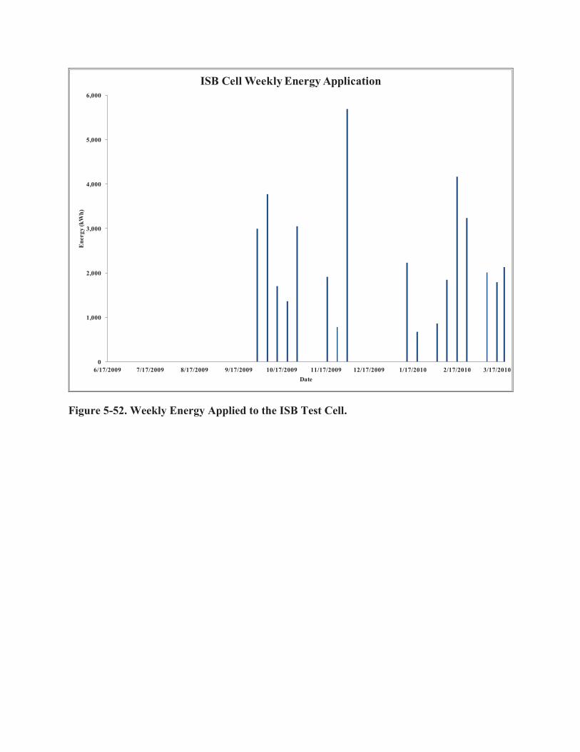
0
1,000
2,000
3,000
4,000
5,000
6,000
6/17/2009 7/17/2009 8/17/2009 9/17/2009 10/17/2009 11/17/2009 12/17/2009 1/17/2010 2/17/2010 3/17/2010
Ene
rgy
(kW
h)
Date
ISB Cell Weekly Energy Application
Figure 5-52. Weekly Energy Applied to the ISB Test Cell.
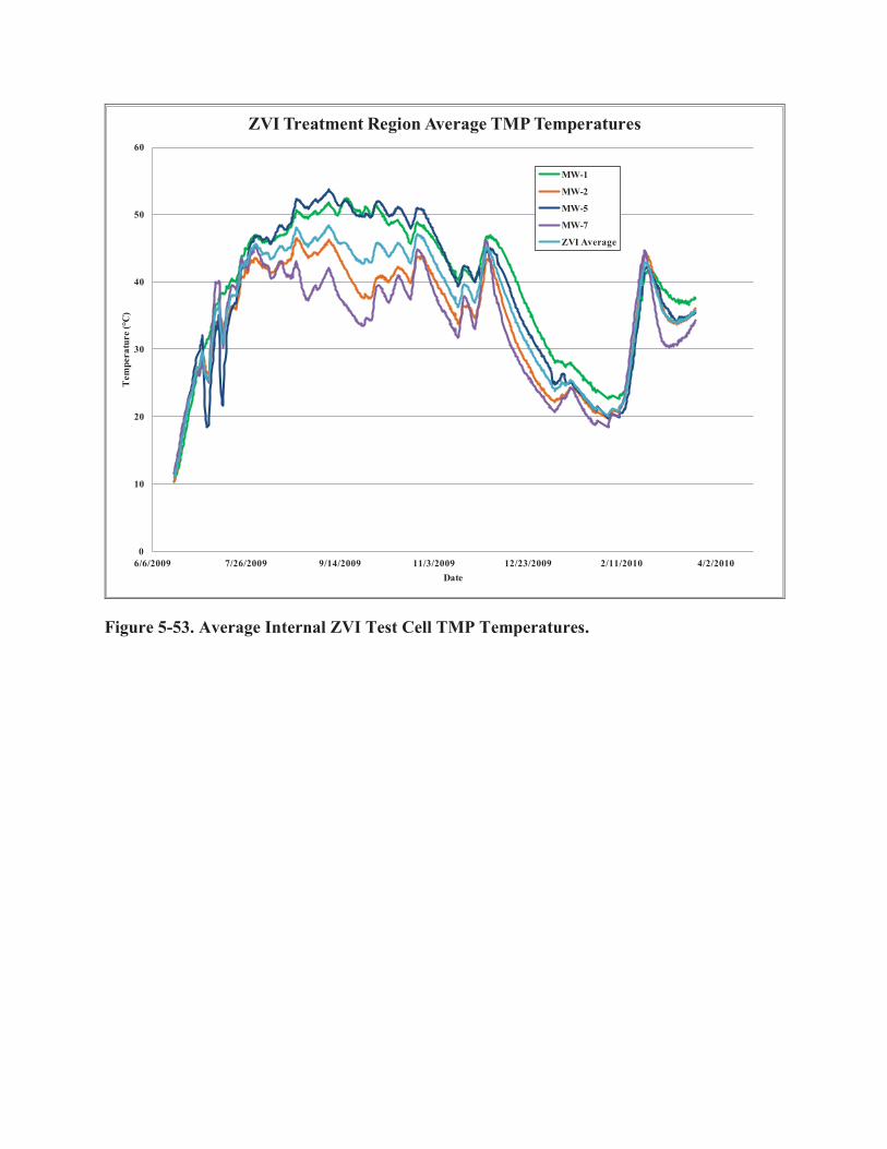
0
10
20
30
40
50
60
6/6/2009 7/26/2009 9/14/2009 11/3/2009 12/23/2009 2/11/2010 4/2/2010
Tem
pera
ture
(°C
)
Date
ZVI Treatment Region Average TMP Temperatures
MW-1
MW-2
MW-5
MW-7
ZVI Average
Figure 5-53. Average Internal ZVI Test Cell TMP Temperatures.
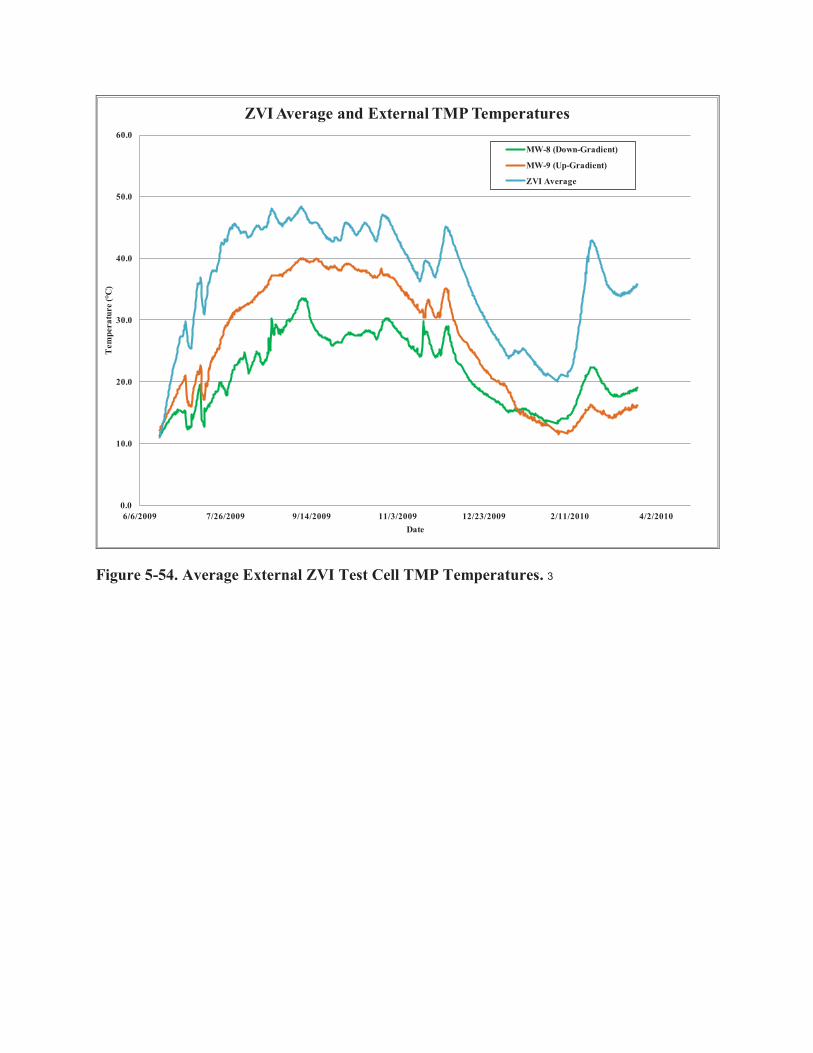
0.0
10.0
20.0
30.0
40.0
50.0
60.0
6/6/2009 7/26/2009 9/14/2009 11/3/2009 12/23/2009 2/11/2010 4/2/2010
Tem
pera
ture
(°C
)
Date
ZVI Average and External TMP Temperatures
MW-8 (Down-Gradient)
MW-9 (Up-Gradient)
ZVI Average
Figure 5-54. Average External ZVI Test Cell TMP Temperatures. 3
Section 5 • Test Design
141 ESTCP ER-0719 Final Report
ISB-MW3 allowing it to reach 30°C within 5 days of operation. The PCU output configuration was changed immediately, with the electrode nearest the MW disconnected from the array, to address the preferential heating near ISB-MW3 and Phase 3 operations were continued in the ISB test cell.
By October 24, 2009, the average ISB test cell temperature had reached the lower limit of the desired temperature range (30-40°C) for the first time. During this period, the average subsurface temperature increased at a rate of 0.7°C per day. The ISB average subsurface heat-up rate was also increased at a rate to achieve project objectives in a timely manner but slow enough to avoid the volatilization of subsurface components with the treatment region.
The average subsurface temperatures in ISB-MW1 and ISB-MW2 remained in the desired temperature range for the next 154 days of operation until the end of Phase-3 operations on March 22, 2010.
Observed temperatures in the down-gradient external ISB TMP locations also parallel trends normally observed at ERH sites where no hydraulic control exists. The upgradient TMP for the ISB test cell, ISB-INJ, displays wide shifts of temperature that are associated with the injections performed within the ISB test cell at ISB-INJ. The temperature of the injected solution either increased the observed subsurface temperature during summer months or decreased the observed temperature during winter months due to storage in above grade ambient temperatures.
Internal and external ISB test cell average temperatures are shown in Figure 5-55 and Figure 5-56 respectively.
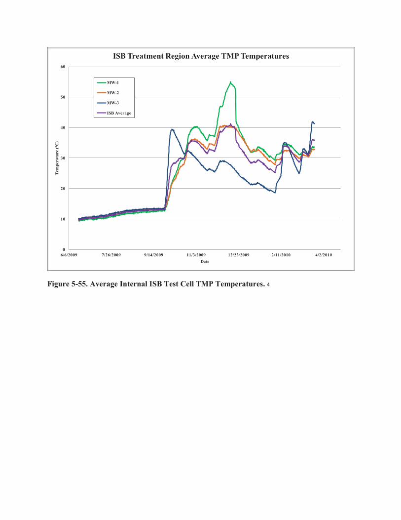
0
10
20
30
40
50
60
6/6/2009 7/26/2009 9/14/2009 11/3/2009 12/23/2009 2/11/2010 4/2/2010
Tem
pera
ture
(°C
)
Date
ISB Treatment Region Average TMP Temperatures
MW-1
MW-2
MW-3
ISB Average
Figure 5-55. Average Internal ISB Test Cell TMP Temperatures. 4

0.0
5.0
10.0
15.0
20.0
25.0
30.0
35.0
40.0
45.0
6/6/2009 7/26/2009 9/14/2009 11/3/2009 12/23/2009 2/11/2010 4/2/2010
Tem
pera
ture
(°C
)
Date
ISB Average and External TMP Temperatures
MW-4 (Down-Gradient)
MW-5 (Down-Gradient)
MW-6 (Down-Gradient)
ISB Average
INJ (Up-Gradient)
Figure 5-56. Average External ISB Test Cell TMP Temperatures. 5
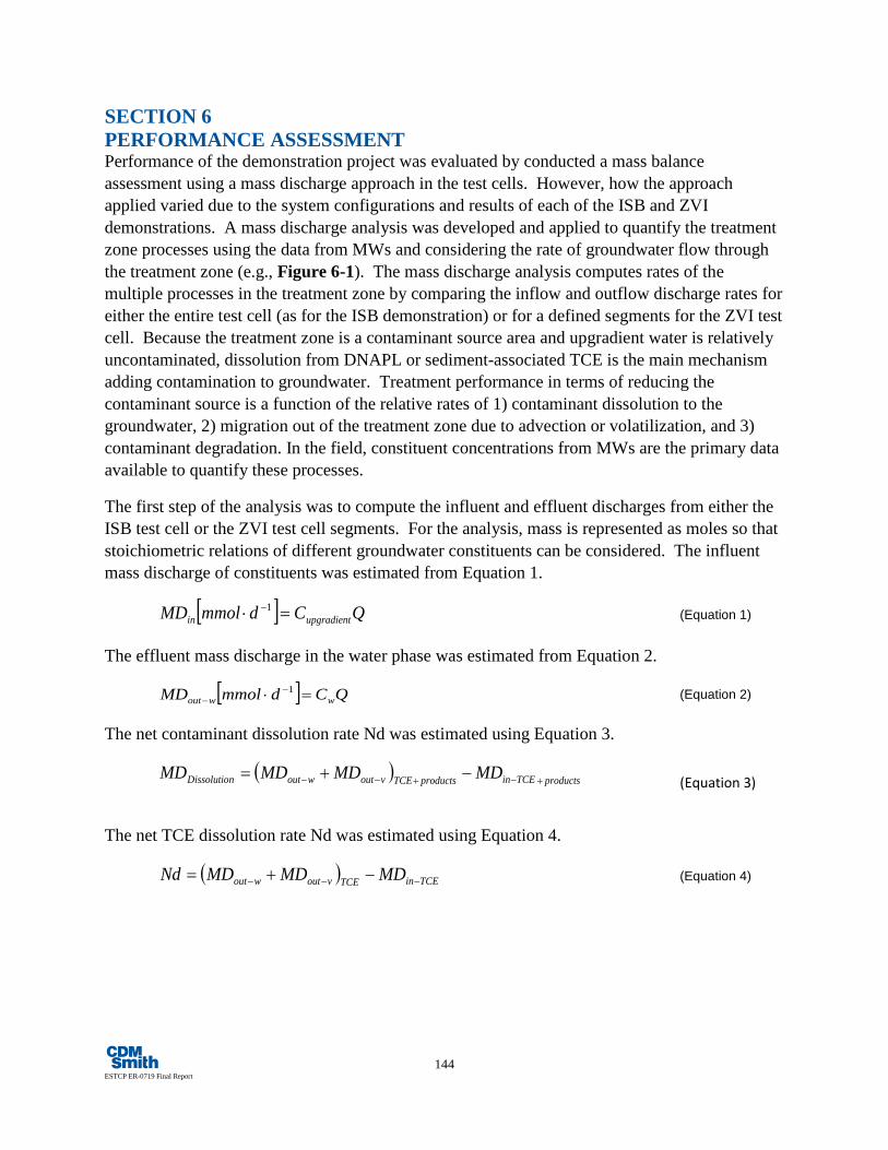
144 ESTCP ER-0719 Final Report
SECTION 6 PERFORMANCE ASSESSMENT Performance of the demonstration project was evaluated by conducted a mass balance assessment using a mass discharge approach in the test cells. However, how the approach applied varied due to the system configurations and results of each of the ISB and ZVI demonstrations. A mass discharge analysis was developed and applied to quantify the treatment zone processes using the data from MWs and considering the rate of groundwater flow through the treatment zone (e.g., Figure 6-1). The mass discharge analysis computes rates of the multiple processes in the treatment zone by comparing the inflow and outflow discharge rates for either the entire test cell (as for the ISB demonstration) or for a defined segments for the ZVI test cell. Because the treatment zone is a contaminant source area and upgradient water is relatively uncontaminated, dissolution from DNAPL or sediment-associated TCE is the main mechanism adding contamination to groundwater. Treatment performance in terms of reducing the contaminant source is a function of the relative rates of 1) contaminant dissolution to the groundwater, 2) migration out of the treatment zone due to advection or volatilization, and 3) contaminant degradation. In the field, constituent concentrations from MWs are the primary data available to quantify these processes.
The first step of the analysis was to compute the influent and effluent discharges from either the ISB test cell or the ZVI test cell segments. For the analysis, mass is represented as moles so that stoichiometric relations of different groundwater constituents can be considered. The influent mass discharge of constituents was estimated from Equation 1.
[ ] QCdmmolMD upgradientin =⋅ −1 (Equation 1)
The effluent mass discharge in the water phase was estimated from Equation 2.
[ ] QCdmmolMD wwout =⋅ −−
1 (Equation 2)
The net contaminant dissolution rate Nd was estimated using Equation 3.
( ) productsTCEinproductsTCEvoutwoutnDissolutio MDMDMDMD +−+−− −+= (Equation 3)
The net TCE dissolution rate Nd was estimated using Equation 4.
( ) TCEinTCEvoutwout MDMDMDNd −−− −+= (Equation 4)

Figure 6-1. Mass-discharge analysis configuration where MDin is the influent mass discharge and MDout-w and MDout-v are the effluent mass discharge in the water and vapor phases, respectively (Truex et al. 2011).
MDout-v
MDout-w
MDin
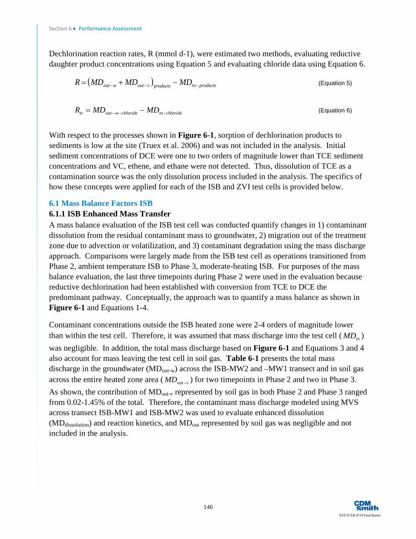
Section 6 • Performance Assessment
146
ESTCP ER-0719 Final Report
Dechlorination reaction rates, R (mmol d-1), were estimated two methods, evaluating reductive daughter product concentrations using Equation 5 and evaluating chloride data using Equation 6.
( ) productsinproductsvoutwout MDMDMDR −−− −+= (Equation 5)
chlorideinchloridewouttc MDMDR −−− −= (Equation 6)
With respect to the processes shown in Figure 6-1, sorption of dechlorination products to sediments is low at the site (Truex et al. 2006) and was not included in the analysis. Initial sediment concentrations of DCE were one to two orders of magnitude lower than TCE sediment concentrations and VC, ethene, and ethane were not detected. Thus, dissolution of TCE as a contamination source was the only dissolution process included in the analysis. The specifics of how these concepts were applied for each of the ISB and ZVI test cells is provided below.
6.1 Mass Balance Factors ISB 6.1.1 ISB Enhanced Mass Transfer A mass balance evaluation of the ISB test cell was conducted quantify changes in 1) contaminant dissolution from the residual contaminant mass to groundwater, 2) migration out of the treatment zone due to advection or volatilization, and 3) contaminant degradation using the mass discharge approach. Comparisons were largely made from the ISB test cell as operations transitioned from Phase 2, ambient temperature ISB to Phase 3, moderate-heating ISB. For purposes of the mass balance evaluation, the last three timepoints during Phase 2 were used in the evaluation because reductive dechlorination had been established with conversion from TCE to DCE the predominant pathway. Conceptually, the approach was to quantify a mass balance as shown in Figure 6-1 and Equations 1-4.
Contaminant concentrations outside the ISB heated zone were 2-4 orders of magnitude lower than within the test cell. Therefore, it was assumed that mass discharge into the test cell ( inMD ) was negligible. In addition, the total mass discharge based on Figure 6-1 and Equations 3 and 4 also account for mass leaving the test cell in soil gas. Table 6-1 presents the total mass discharge in the groundwater (MDout-w) across the ISB-MW2 and –MW1 transect and in soil gas across the entire heated zone area ( voutMD − ) for two timepoints in Phase 2 and two in Phase 3. As shown, the contribution of MDout-v represented by soil gas in both Phase 2 and Phase 3 ranged from 0.02-1.45% of the total. Therefore, the contaminant mass discharge modeled using MVS across transect ISB-MW1 and ISB-MW2 was used to evaluate enhanced dissolution (MDdissolution) and reaction kinetics, and MDout represented by soil gas was negligible and not included in the analysis.
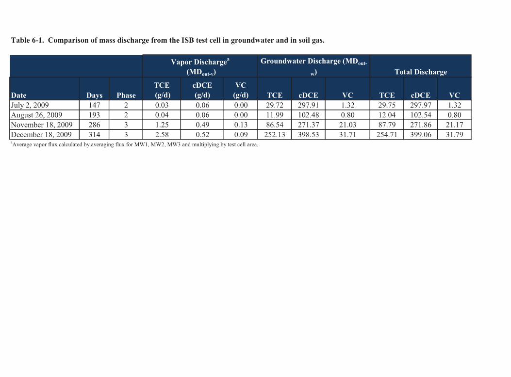
Table 6-1. Comparison of mass discharge from the ISB test cell in groundwater and in soil gas.
Date Days PhaseTCE (g/d)
cDCE (g/d)
VC(g/d) TCE cDCE VC TCE cDCE VC
July 2, 2009 147 2 0.03 0.06 0.00 29.72 297.91 1.32 29.75 297.97 1.32August 26, 2009 193 2 0.04 0.06 0.00 11.99 102.48 0.80 12.04 102.54 0.80November 18, 2009 286 3 1.25 0.49 0.13 86.54 271.37 21.03 87.79 271.86 21.17December 18, 2009 314 3 2.58 0.52 0.09 252.13 398.53 31.71 254.71 399.06 31.79aAverage vapor flux calculated by averaging flux for MW1, MW2, MW3 and multiplying by test cell area.
Vapor Dischargea
(MDout-v)Groundwater Discharge (MDout-
w) Total Discharge
195

Section 6 • Performance Assessment
148
ESTCP ER-0719 Final Report
To calculate mass flux and mass discharge, hydraulic conductivity data and groundwater elevation data were input into the 3D MVS software to establish a 3D groundwater flow field for three timepoints during Phase 2 (days 92, 147 and 193) and six timepoints during Phase 3 (days 251, 286, 314, 355, 384, 411). The average horizontal hydraulic conductivity measured at ISB-MW1 and ISB-MW2 for each of three depth intervals (approximately 12, 17 and 22 ft bgs) was used (Table 5-7). The vertical hydraulic conductivity was set at half the magnitude of the horizontal hydraulic conductivity. Groundwater elevation and contaminant concentrations measured at each timepoint were then input into the model and kriged in three dimensions. Groundwater contaminant mass flux was then calculated in three dimensions and a transect set through ISB-MW2 and -MW1 was used to evaluate mass discharge by integrating the mass flux values over the transect area (approximately 16 ft wide by 21 ft deep). This was used to develop the estimates for MDout for total VOCs (TCE + products), reductive daughter products (DCE, VC, ethene) and chloride.
The total VOCs dissolution rate (MDdissolution), reaction rate using daughter products (R) and reaction rates using chloride (Rtc) over the course of the demonstration, shown in Figure 5-24 and Table 5-20, was plotted as a function of temperature (Figure 6-2). These data indicate a positive correlation for MDdissolution (R2 = 0.53), R (R2=0.45) and Rtc (R2=0.60) as a function of temperature from the test cell.
The MDdissolution due to heating in Phase 3 was evaluated by comparing MDout of total VOCs as a function of temperature. For this analysis, the influent MDin and vapor MDin-vapor were assumed negligible. Based on the correlation in Figure 6-2, the total VOC dissolution increases by a factor of 4.6, or an increase from 177 g VOC as TCE/d to 812 g VOC as TCE/d when temperatures are increased from 10⁰C to 40⁰C. The increase is largely attributed to enhanced mass transfer due to the elevated temperature as opposed to reductive dechlorination reactions (i.e. enhancing the concentration gradient due to removal parent compounds and formation of daughter products) because the comparison was made between Phase 2, where dechlorination reactions had already been established at ambient temperatures and Phase 3.This is in good agreement with Imhoff et al 1997, which described the enhanced dissolution of TCE DNAPLs during hot water flushing. In this work the aqueous phase mass transfer coefficient, Ka, was developed experimentally and results applied to empirical model. Increasing temperatures from 10⁰C to 35⁰C increased in Ka by a factor of 2 and by 3 when temperatures increased to 55⁰C. These data suggest that significant enhanced dissolution occurs within areas containing DNAPLs at elevated temperatures.
6.1.2 ISB Impact of Elevated Temperature on Kinetics To evaluate the impact of heating on treatment rates of TCE, the rate (R) was evaluated using Equations 4 and 5. First the reaction rate was estimated using reductive daughter products where MDout of reductive daughter products was evaluated and used as the reaction rate, R (mmol/d). For this analysis, the influent MDin and vapor MDin-vapor were assumed negligible. Based on the correlation developed in Figure 6-2, the R estimated increased by a factor of 3.6 when you
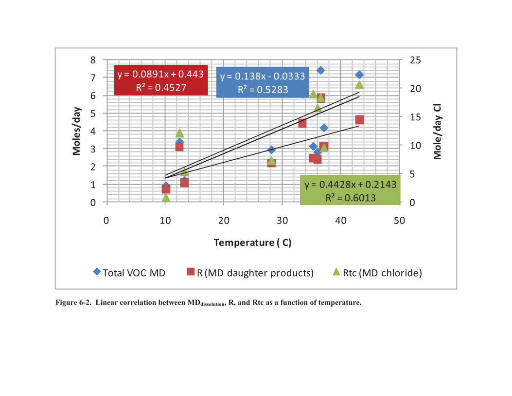
Figure 6-2. Linear correlation between MDdissolution, R, and Rtc as a function of temperature.
y = 0.138x - 0.0333R² = 0.5283
y = 0.0891x + 0.443R² = 0.4527
y = 0.4428x + 0.2143R² = 0.6013 0
5
10
15
20
25
0
1
2
3
4
5
6
7
8
0 10 20 30 40 50
Mol
e/da
y Cl
Mol
es/d
ay
Temperature ( C)
Total VOC MD R (MD daughter products) Rtc (MD chloride)
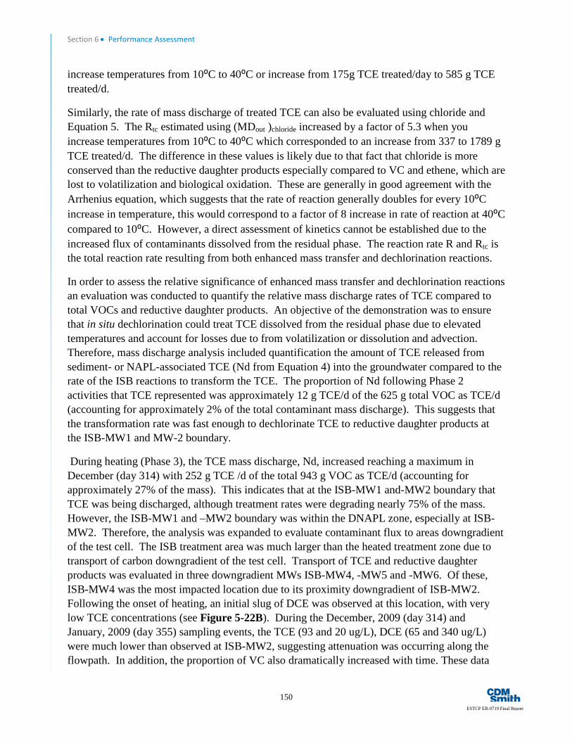
Section 6 • Performance Assessment
150
ESTCP ER-0719 Final Report
increase temperatures from 10⁰C to 40⁰C or increase from 175g TCE treated/day to 585 g TCE treated/d.
Similarly, the rate of mass discharge of treated TCE can also be evaluated using chloride and Equation 5. The Rtc estimated using (MDout )chloride increased by a factor of 5.3 when you increase temperatures from 10⁰C to 40⁰C which corresponded to an increase from 337 to 1789 g TCE treated/d. The difference in these values is likely due to that fact that chloride is more conserved than the reductive daughter products especially compared to VC and ethene, which are lost to volatilization and biological oxidation. These are generally in good agreement with the Arrhenius equation, which suggests that the rate of reaction generally doubles for every 10⁰C increase in temperature, this would correspond to a factor of 8 increase in rate of reaction at 40⁰C compared to 10⁰C. However, a direct assessment of kinetics cannot be established due to the increased flux of contaminants dissolved from the residual phase. The reaction rate R and Rtc is the total reaction rate resulting from both enhanced mass transfer and dechlorination reactions.
In order to assess the relative significance of enhanced mass transfer and dechlorination reactions an evaluation was conducted to quantify the relative mass discharge rates of TCE compared to total VOCs and reductive daughter products. An objective of the demonstration was to ensure that in situ dechlorination could treat TCE dissolved from the residual phase due to elevated temperatures and account for losses due to from volatilization or dissolution and advection. Therefore, mass discharge analysis included quantification the amount of TCE released from sediment- or NAPL-associated TCE (Nd from Equation 4) into the groundwater compared to the rate of the ISB reactions to transform the TCE. The proportion of Nd following Phase 2 activities that TCE represented was approximately 12 g TCE/d of the 625 g total VOC as TCE/d (accounting for approximately 2% of the total contaminant mass discharge). This suggests that the transformation rate was fast enough to dechlorinate TCE to reductive daughter products at the ISB-MW1 and MW-2 boundary.
During heating (Phase 3), the TCE mass discharge, Nd, increased reaching a maximum in December (day 314) with 252 g TCE /d of the total 943 g VOC as TCE/d (accounting for approximately 27% of the mass). This indicates that at the ISB-MW1 and-MW2 boundary that TCE was being discharged, although treatment rates were degrading nearly 75% of the mass. However, the ISB-MW1 and –MW2 boundary was within the DNAPL zone, especially at ISB-MW2. Therefore, the analysis was expanded to evaluate contaminant flux to areas downgradient of the test cell. The ISB treatment area was much larger than the heated treatment zone due to transport of carbon downgradient of the test cell. Transport of TCE and reductive daughter products was evaluated in three downgradient MWs ISB-MW4, -MW5 and -MW6. Of these, ISB-MW4 was the most impacted location due to its proximity downgradient of ISB-MW2. Following the onset of heating, an initial slug of DCE was observed at this location, with very low TCE concentrations (see Figure 5-22B). During the December, 2009 (day 314) and January, 2009 (day 355) sampling events, the TCE (93 and 20 ug/L), DCE (65 and 340 ug/L) were much lower than observed at ISB-MW2, suggesting attenuation was occurring along the flowpath. In addition, the proportion of VC also dramatically increased with time. These data

Section 6 • Performance Assessment
151 ESTCP ER-0719 Final Report
suggest that although TCE was mobilized, that it could be mitigated, and treated, by creating a sufficiently large treatment area downgradient of the source zone to ensure treatment of mobilized TCE.
6.2 Mass Balance Factors ZVI 6.2.1 ZVI Mass Transfer A mass balance/mass discharge analysis was applied to evaluate TCE dechlorination, dissolution, advection, and volatilization in the ZVI test cell. The analysis was designed to account for the ZVI distribution and hydraulic conditions in the test cell. Key considerations are described below.
ZVI mass in the test cell was highest surrounding the injection well (Truex et al. 2010). The ZVI test cell was centered on a high TCE contamination zone surrounded by groundwater at much lower TCE concentrations. Additionally, ZVI was distributed to the test cell using SlurryPro™, a shear-thinning fluid, which when static has a high viscosity (Truex et al. 2010). Data suggest that the groundwater flow rate through the ZVI test cell was much slower than the flow rate prior to injection of the ZVI and SlurryPro™, with a nominal post-injection value based on tracer elution of 0.38 m/d (Truex et al. 2010, 2011). While the flow rate could not be evaluated over the course of the test, test data do not suggest a large change in flow rate during the test. If a change were to occur, it would have increased the flow rate over time as the viscosity of the SlurryPro™ decreased due to dispersal or degradation. Thus, comparison of rates between initial Phase 2 ambient temperature operation and Phase 3 heated operations would tend to be conservative and underestimate rates in Phase 3 versus Phase 2 if the groundwater flow rate increased over time.
Based on the above considerations, the mass discharge (moles per time) was estimated for assigned test cell segments through well INJ as shown on Figure 6-1. The mass discharge analysis was applied to evaluate dechlorination in this segment along a flow path through the center of the test cell. This segments fall along the nominal flow path of groundwater through the test cell that intersects the zone of highest ZVI concentration (i.e., surrounding the injection well). The longitudinal dimension of the segment was based on the estimated distance to the edge of the ZVI/SlurryPro™ injection. The segment used a unit lateral dimension of 1 m and a thickness equal to the well screen interval (1.5 m).
The mass discharge analysis is presented in Truex et al. 2011 and repeated here. A mass-discharge analysis was developed and applied to quantify the treatment zone processes using the data from MWs and considering the rate of groundwater flow through the treatment zone segments ending at each MW (Figure 6-3). The mass-discharge analysis computes rates of the multiple processes in the treatment zone by comparing the inflow and outflow discharge rates for a defined segment as shown in Figure 6-3. Because the treatment zone is a contaminant source area and upgradient water is relatively uncontaminated, dissolution from DNAPL or sediment-associated TCE is the main mechanism adding contamination to groundwater. Treatment performance in terms of reducing the contaminant source is a function of the relative rates of 1) contaminant dissolution to the groundwater, 2) contaminant degradation, and 3) migration out of

Figure 6-3. Calculated TCE reaction rates and Nd for the INJ segment (Truex etal. 2011).
0
10
20
30
40
50
-1
0
1
2
3
4
5
6
0 30 60 90 120 150
Tem
pera
ture
(C)
Cal
cula
ted
Rea
ctio
n R
ates
an
d N
d (m
mol
e d-
1 )
Time from ZVI Injection (days)
RtRbRaNdTemperature

Section 6 • Performance Assessment
153 ESTCP ER-0719 Final Report
the treatment zone due to advection or volatilization. In the field, constituent concentrations from MWs are the primary data available to quantify these processes. Additionally, a source area treatment analysis is unlike an analysis for a permeable reactive barrier where the primary goal is reduction of upgradient contaminants as they flow through the treatment zone.
The first step of the analysis was to compute the influent and effluent discharges of the segments. For the analysis, mass is represented as moles so that stoichiometric relations of different groundwater constituents can be considered. The influent mass discharge of constituents to each segment was estimated from Equation 1 where Cupgradient [mmol L-1] is the concentration at well ZVI-MW9. Data for well ZVI-MW9 was assumed to represent conditions upgradient of the test cell because the ZVI injection did not reach this well (Truex et al. 2010). A groundwater flow rate, Q, of 103 L/d was calculated from the estimated linear velocity, porosity (0.18), and cross section area of the segments using Darcy’s Law and assumed to remain constant. The effluent mass discharge in the water phase was estimated from Equation 2 where Cw [mmol/L] is the concentration at the MWs for the selected segments.
The effluent mass discharge in the vapor phase was estimated from Equation 6.
[ ]
=⋅ −
−v
wvasvout L
HCADdmmolMD 1 (Equation 6)
The diffusion coefficient for each compound in sediment, Das, was calculated from the individual gas diffusion coefficients (Yaws 2003) (T=25oC) using the method of Millington and Quirk (1961), the measured porosity, and moisture content (14.5%[v/v]). The dimensionless Henry’s Law coefficient, H, corrected for temperature was calculated for each compound from tabulated vapor pressure (Yaws 2009) and solubility data (Yaws 2009; Mackay et al. 2006) as a function of temperature. The distance from the water table to the ground surface, Lv, was estimated as the average vadose zone thickness of 2.13 m. The surface area for diffusive mass transfer, Av, was based on the distance from the upgradient edge of the treatment zone to the MW with a unit width of 1 m. Soil gas data were not used in the analysis because pre-test vapor-phase TCE and DCE concentrations were an average of 69 and 15 times higher, respectively, in samples from the unsaturated sand pack of wells ZVI-MW2 through -MW7 than vapor concentrations calculated based on the measured groundwater concentration and equilibrium partitioning by Henry’s Law. These data indicated the presence of significant vadose zone contamination that would interfere with directly measuring volatilization of TCE and DCE from the groundwater.
The next phase of the analysis relates the segment inflow and outflow of groundwater constituents, computed using Equations 1-3, to the rates of reactions and processes occurring in these segments. This approach enables estimation of the overall TCE dissolution and degradation rates, the amount of TCE released from the source but untreated, and the reaction rates producing specific reaction products as a function of the conditions within the test cell (e.g.,

Section 6 • Performance Assessment
154
ESTCP ER-0719 Final Report
temperature). These segment reaction rates define the treatment performance and, along with the ZVI amendment information, can be used for process scale-up and performance estimation.
When all organic dechlorination products were considered, the estimated reaction rate from Equation 4 represents the overall rate of TCE transformation, Rt. An abiotic reaction rate, Ra (elimination reaction), was estimated using Equation 4 by only considering transformation to ethene, ethane, and acetylene products. A biotic reaction rate, Rb, was estimated using Equation 4 by only considering transformation to DCE as the product, representing the combined effect of both biotic and direct ZVI hydrogenolysis reactions. Because negligible VC was observed during the test (3 to 4 orders of magnitude lower concentrations than DCE), it was assumed that biological dechlorination converted TCE to DCE only. One could consider Ra as representing the sum of reactions that produce non-hazardous products and Rb as DCE-producing reactions. The actual reactions occurring in the treatment zone are likely a mix of biotic and abiotic reactions. For instance, ZVI degrades DCE and VC, though at lower rates than TCE. Additionally, some biotic dechlorination beyond DCE is possible, though unlikely due to low observed VC concentrations. Molecular DNA data targeting Dehalococcoides, the bacteria that converts cis-DCE to ethene, remained at low levels during the test, generally below the threshold concentration of 106 gene copy/ L to observe significant complete biotic dechlorination at JBLM groundwater (Macbeth and Sorenson, ESTCP ER-0318 Final Report), indicating biotic cis-DCE dechlorination was limited (Truex et al. 2011).
The overall rate of TCE dechlorination was also estimated using chloride data, Rtc (mmol d-1), using Equation 5. To convert chloride data to the equivalent moles of TCE, the chloride stoichiometry can be assigned based on the relative molar amounts of DCE, ethene, and ethane products observed at each time point.
6.2.2 ZVI Kinetic Changes The impact of temperature on the in situ dechlorination reactions induced by injected ZVI are reported in Truex et al. (2011) and detailed here. A mass discharge analysis was used to evaluate the performance of the treatment with respect to dechlorination as a function of temperature. Due to seasonal variation, the water level declined such that a portion of the screen was unsaturated starting at about day 121 reaching a minimum of 70% saturated thickness by day 184. Because of this large change in hydrologic conditions, and the fact that the majority of TCE residual mass in the ZVI test cell was largely at the water table, the dechlorination rate analysis was constrained to data over the first 121 days of treatment.
Figure 6-3 shows the calculated TCE dechlorination rates and released but untreated TCE (Nd) over the first 121 days for the INJ segment. Flow paths through the test cell are uncertain. However, the INJ segment represents flow from upgradient through the zone of highest ZVI concentration.
Abiotic reactions predominate in the INJ segment. For the INJ segment, overall TCE transformation, Rt was 3.6-4.8 times higher at temperatures above 30°C compared to rates at the ambient temperature (~10°C). This result is consistent with laboratory tests where the TCE
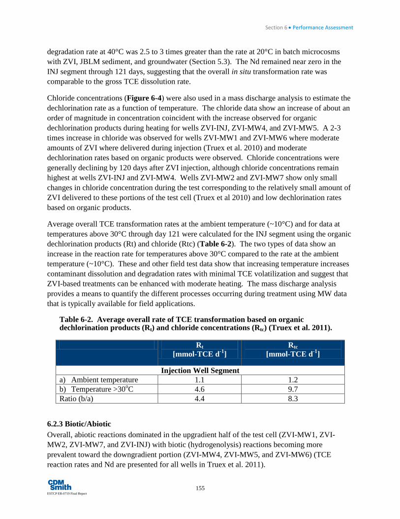
Section 6 • Performance Assessment
155 ESTCP ER-0719 Final Report
degradation rate at 40°C was 2.5 to 3 times greater than the rate at 20°C in batch microcosms with ZVI, JBLM sediment, and groundwater (Section 5.3). The Nd remained near zero in the INJ segment through 121 days, suggesting that the overall in situ transformation rate was comparable to the gross TCE dissolution rate.
Chloride concentrations (Figure 6-4) were also used in a mass discharge analysis to estimate the dechlorination rate as a function of temperature. The chloride data show an increase of about an order of magnitude in concentration coincident with the increase observed for organic dechlorination products during heating for wells ZVI-INJ, ZVI-MW4, and ZVI-MW5. A 2-3 times increase in chloride was observed for wells ZVI-MW1 and ZVI-MW6 where moderate amounts of ZVI where delivered during injection (Truex et al. 2010) and moderate dechlorination rates based on organic products were observed. Chloride concentrations were generally declining by 120 days after ZVI injection, although chloride concentrations remain highest at wells ZVI-INJ and ZVI-MW4. Wells ZVI-MW2 and ZVI-MW7 show only small changes in chloride concentration during the test corresponding to the relatively small amount of ZVI delivered to these portions of the test cell (Truex et al 2010) and low dechlorination rates based on organic products.
Average overall TCE transformation rates at the ambient temperature (~10°C) and for data at temperatures above 30°C through day 121 were calculated for the INJ segment using the organic dechlorination products (Rt) and chloride (Rtc) (Table 6-2). The two types of data show an increase in the reaction rate for temperatures above 30°C compared to the rate at the ambient temperature (~10°C). These and other field test data show that increasing temperature increases contaminant dissolution and degradation rates with minimal TCE volatilization and suggest that ZVI-based treatments can be enhanced with moderate heating. The mass discharge analysis provides a means to quantify the different processes occurring during treatment using MW data that is typically available for field applications.
Table 6-2. Average overall rate of TCE transformation based on organic dechlorination products (Rt) and chloride concentrations (Rtc) (Truex et al. 2011).
Rt [mmol-TCE d-1]
Rtc [mmol-TCE d-1]
Injection Well Segment a) Ambient temperature 1.1 1.2 b) Temperature >30oC 4.6 9.7 Ratio (b/a) 4.4 8.3
6.2.3 Biotic/Abiotic Overall, abiotic reactions dominated in the upgradient half of the test cell (ZVI-MW1, ZVI-MW2, ZVI-MW7, and ZVI-INJ) with biotic (hydrogenolysis) reactions becoming more prevalent toward the downgradient portion (ZVI-MW4, ZVI-MW5, and ZVI-MW6) (TCE reaction rates and Nd are presented for all wells in Truex et al. 2011).

0
10
20
30
40
50
0
5
10
15
20
25
30
35
0 30 60 90 120 150
Tem
pera
ture
(C
)
Chl
orid
e (m
g L-1
)
Days After ZVI Injection
INJMW1MW2MW4MW5MW6MW7MW8MW9T at INJ
Figure 6-4. Chloride concentration over time in the ZVI test cell. Wells MW8 and MW9 are outside the injection zone, although a small amount of ZVI was distributed to MW8 during injection (Truex et al. 2011).
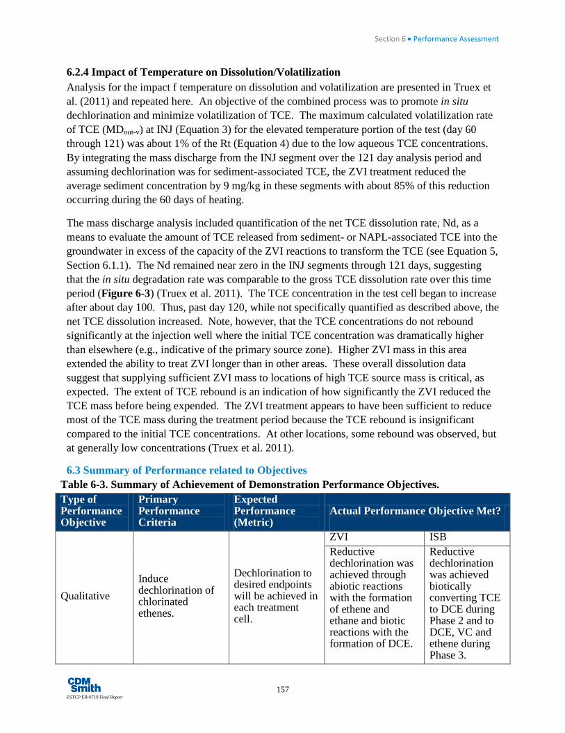
Section 6 • Performance Assessment
157 ESTCP ER-0719 Final Report
6.2.4 Impact of Temperature on Dissolution/Volatilization Analysis for the impact f temperature on dissolution and volatilization are presented in Truex et al. (2011) and repeated here. An objective of the combined process was to promote in situ dechlorination and minimize volatilization of TCE. The maximum calculated volatilization rate of TCE (MDout-v) at INJ (Equation 3) for the elevated temperature portion of the test (day 60 through 121) was about 1% of the Rt (Equation 4) due to the low aqueous TCE concentrations. By integrating the mass discharge from the INJ segment over the 121 day analysis period and assuming dechlorination was for sediment-associated TCE, the ZVI treatment reduced the average sediment concentration by 9 mg/kg in these segments with about 85% of this reduction occurring during the 60 days of heating.
The mass discharge analysis included quantification of the net TCE dissolution rate, Nd, as a means to evaluate the amount of TCE released from sediment- or NAPL-associated TCE into the groundwater in excess of the capacity of the ZVI reactions to transform the TCE (see Equation 5, Section 6.1.1). The Nd remained near zero in the INJ segments through 121 days, suggesting that the in situ degradation rate was comparable to the gross TCE dissolution rate over this time period (Figure 6-3) (Truex et al. 2011). The TCE concentration in the test cell began to increase after about day 100. Thus, past day 120, while not specifically quantified as described above, the net TCE dissolution increased. Note, however, that the TCE concentrations do not rebound significantly at the injection well where the initial TCE concentration was dramatically higher than elsewhere (e.g., indicative of the primary source zone). Higher ZVI mass in this area extended the ability to treat ZVI longer than in other areas. These overall dissolution data suggest that supplying sufficient ZVI mass to locations of high TCE source mass is critical, as expected. The extent of TCE rebound is an indication of how significantly the ZVI reduced the TCE mass before being expended. The ZVI treatment appears to have been sufficient to reduce most of the TCE mass during the treatment period because the TCE rebound is insignificant compared to the initial TCE concentrations. At other locations, some rebound was observed, but at generally low concentrations (Truex et al. 2011).
6.3 Summary of Performance related to Objectives Table 6-3. Summary of Achievement of Demonstration Performance Objectives. Type of Performance Objective
Primary Performance Criteria
Expected Performance (Metric)
Actual Performance Objective Met?
Qualitative Induce dechlorination of chlorinated ethenes.
Dechlorination to desired endpoints will be achieved in each treatment cell.
ZVI ISB Reductive dechlorination was achieved through abiotic reactions with the formation of ethene and ethane and biotic reactions with the formation of DCE.
Reductive dechlorination was achieved biotically converting TCE to DCE during Phase 2 and to DCE, VC and ethene during Phase 3.

Section 6 • Performance Assessment
158
ESTCP ER-0719 Final Report
Table 6-3. Summary of Achievement of Demonstration Performance Objectives. Type of Performance Objective
Primary Performance Criteria
Expected Performance (Metric)
Actual Performance Objective Met?
Reduction in parent compounds and accumulation of abiotic and/or biotic reductive daughter products.
Biotic contaminant removal will be the primary mechanism at ambient and elevated temperature in the ISB test cell. Abiotic and biotic contaminant removal will be significant in the ZVI test cell at ambient temperature; however, abiotic mechanisms will predominate at elevated temperature.
Abiotic and biotic dechlorination products observed for both ambient and elevated temperature.
Biotic contaminant removal was the primary mechanism at ambient and elevated temperature in the ISB test cell
Quantitative
Characterize nature of contamination with test cell.
Sufficient contaminant mass will be present in both test cells to meet demonstration objectives.
Initial TCE soil concentration averaged 115 mg/kg near INJ, estimated 1 kg total TCE in test cell (10 mg/kg average concentration)
Initial TCE soil concentration averaged 32 mg/kg with maximum concentrations of 130 mg/kg near ISB-MW2.
Define rate of dechlorination as a function of temperature.
The rate of dechlorination will be enhanced at elevated temperature in both test cells relative to ambient temperature.
Rates at T>30C were higher than 10C by a factor of 4 based on dechlorination daughter products and a factor 8 using chloride.
Modeled rates based on empirical correlation at T=40C were higher than 10C by a factor of 3.6 based on dechlorination daughter products and a factor of 5.3 using chloride.
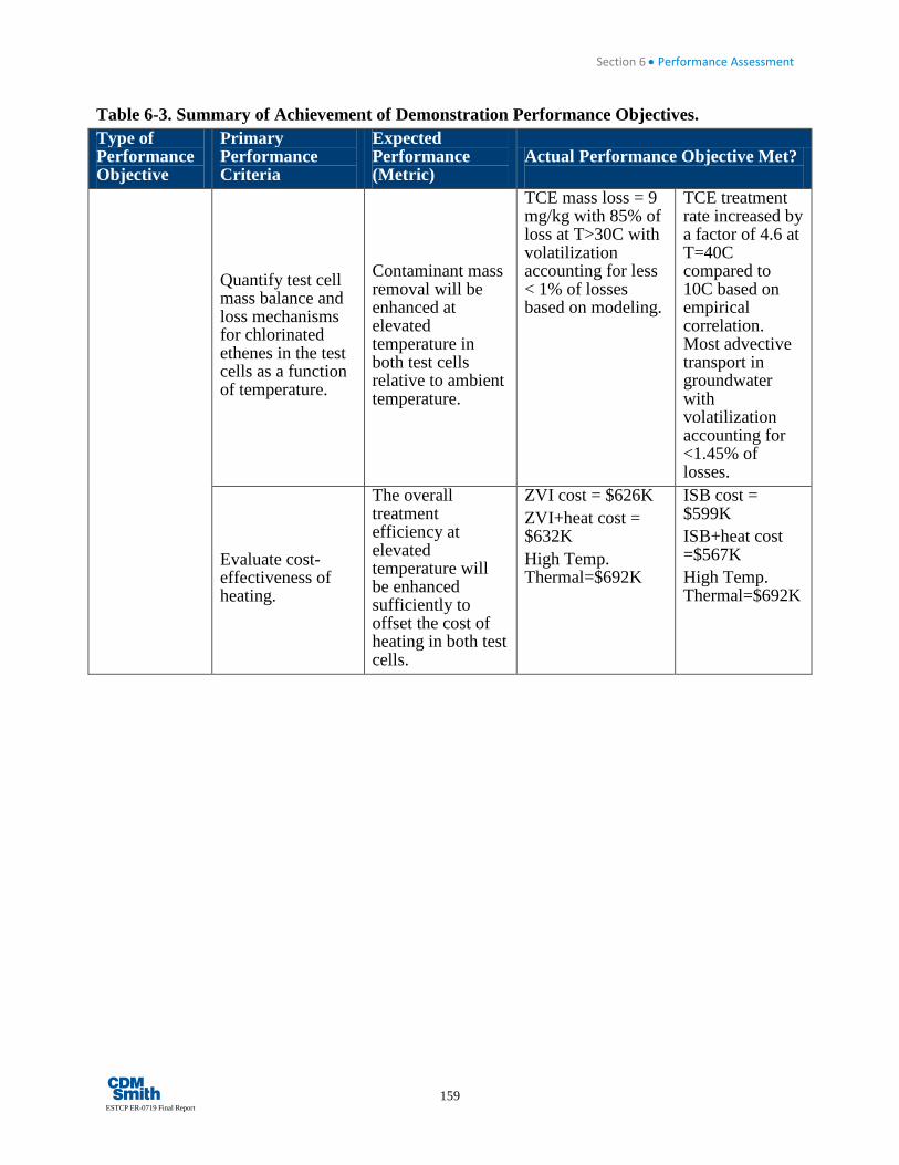
Section 6 • Performance Assessment
159 ESTCP ER-0719 Final Report
Table 6-3. Summary of Achievement of Demonstration Performance Objectives. Type of Performance Objective
Primary Performance Criteria
Expected Performance (Metric)
Actual Performance Objective Met?
Quantify test cell mass balance and loss mechanisms for chlorinated ethenes in the test cells as a function of temperature.
Contaminant mass removal will be enhanced at elevated temperature in both test cells relative to ambient temperature.
TCE mass loss = 9 mg/kg with 85% of loss at T>30C with volatilization accounting for less < 1% of losses based on modeling.
TCE treatment rate increased by a factor of 4.6 at T=40C compared to 10C based on empirical correlation. Most advective transport in groundwater with volatilization accounting for <1.45% of losses.
Evaluate cost-effectiveness of heating.
The overall treatment efficiency at elevated temperature will be enhanced sufficiently to offset the cost of heating in both test cells.
ZVI cost = $626K ZVI+heat cost = $632K High Temp. Thermal=$692K
ISB cost = $599K ISB+heat cost =$567K High Temp. Thermal=$692K

160 ESTCP ER-0719 Final Report
SECTION 7 COST ASSESSMENT 7.1 Cost Model A simplified cost model for the project was developed in order to benefit professionals who may consider similar technology at other sites. The cost model incorporates all technology-specific cost elements required for implementation at a particular site. While costs may vary depending on site size, location, subsurface conditions, etc., the cost model details all the assumptions from which specific cost elements were based. Many of the assumptions pertain to labor expenditure rates and project scale. Figure 7-1 illustrates the assumptions for the ZVI treatment area and system infrastructure used for the cost model. Figure 7-2 illustrates the assumptions for the ISB treatment area and system infrastructure for the cost model. Table 7-1 provides details of the cost model treatment volume. Therefore, professionals wishing to estimate potential costs at other sites may use the cost model developed for this project as a platform to revise with their own unique cost elements and assumptions. To compare the relative costs of the technologies, application of standard, high-temperature thermal treatment to compared to the low-temperature heating coupled to ISB and ZVI was evaluated. In addition, incremental costs for adding low-temperature ISB or ZVI was evaluated under the assumption that high-temperature thermal system was operated. There are several applications for how the technologies could be combined including:
Table 7-1. Cost Assumption Model. Model Treatment Volume Dimensions Treatment Zone Dimensions and Volume n 0.25 -- total porosity estimated from previous data ne 0.18 -- effective porosity from tracer test l 12.2 m treatment zone length w 12.2 m treatment zone width h 9.1 m length of filter pack x sectional area 0 m^2 for total inflow/outflow plan view area 148.7 m^2 for volatilization Vt 1360 m^3 total volume Treatment Zone Mass Bulk dens. 1900 kg/m^3 Total mass 40 kg Ambient Rate 213 g/d Heated Rate 470 g/d Time to Treat 85 days
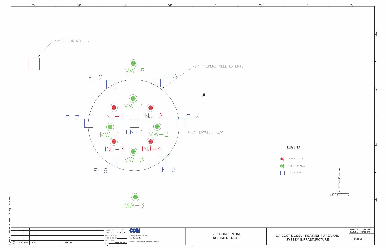


Section 7 • Cost Assessment
163 ESTCP ER-0719 Final Report
Implementation of low-temperature heating with ISB or ZVI as a stand-alone technology,
Implementation of low-temperature heating with ISB or ZVI in conjunction with high-temperature thermal to address areas around the high-temperature thermal treatment zone where it is not cost-effective to treat with high temperature thermal,
Implementation of low-temperature heating with ISB or ZVI in conjunction with high-temperature thermal as a polish following treatment.
To evaluate the technologies, a model system was developed. Table 7-1 provides areal and depth of treatment dimensions of the model system, and a starting target-zone contaminant mass to evaluate treatment rates and durations in the model system. The model assumptions for in situ treatment based on the demonstration are as follows:
Enhanced in situ treatment rates at elevated temperatures were primarily driven by enhanced dissolution due to increased temperatures relative to ambient treatment temperatures,
The in situ treatment technologies can treat contaminants mobilized from the source at temperatures up to 50⁰C effectively in the saturated zone,
Contaminants transported to the vadose zone during low-temperature heating did not require additional treatment to address.
The model treatment zone dimensions are 40 feet (12.2 meters [m]) in length, 40 feet (12.2 m) in width, and 30 feet (9.1 m) in depth, for a total treatment volume of 1,778 cubic yards (1,360 m3). Additionally, an initial chloroethene contaminant mass of 40 kg is assumed. Therefore, one may wish to scale data accordingly if their site is considerably different in size or contains a considerable difference in contaminant mass. Treatment rates were based on modeling for the high temperature thermal and for dissolution of NAPL and with enhancement factors at elevated temperatures demonstrated in this project. The assumptions are as follows:
A high temperature thermal treatment rate of 470 g/d are used to estimate a total treatment duration of 85 days.
Energy consumptions was based on energy consumed during the demonstration for the ISB and ZVI, however, these are conservatively high as Ft. Lewis was a much higher groundwater velocities (and associated heat losses) compared to the model system.
Treatment rates for both ISB and ZVI under ambient temperatures are assumed to be the same. Ambient contaminant discharge rates from the model treatment zone were assumed to be 6 grams of TCE per day (see below for description of assumptions). Therefore, the timeframe for dissolution of all 40 kg of the DNAPL is approximately 11 years assuming that the mass discharge rate is constant.
Section 7 • Cost Assessment
164
ESTCP ER-0719 Final Report
For the low temperature ISB, the enhanced treatment rate factor was assumed to be 6 based on the assumption of a 40⁰C operating temperature, and so 36 grams of TCE per day was assumed. Therefore treatment duration is approximately 1.8 years.
For the low temperature ZVI, the enhanced treatment rate factor was assumed to be a factor of 8 greater than ambient temperatures based on the assumption of a 50⁰C operating temperature, and so 48 grams of TCE per day was assumed. Therefore treatment duration is approximately 1.3 years.
Ambient mass discharge rates out of the treatment zone are:
J=VaC
AJMd ∑=
Where J is the contaminant mass flux, Va is the Darcy velocity, C is the contaminant concentration, Md is the mass discharge and A is the treatment area transect. It is assumed that Va= 0.3 feet per day and average concentration across the treatment zone transect is 1,000 ug/L TCE giving an ambient temperature mass discharge rate of 10 grams TCE per day. Figure 7-3 illustrates the treatment times for the four treatment scenarios using these assumptions.
For each cost element, cost data was tracked during the life cycle of the demonstration, and was captured in the model. Note that some cost elements which were not relevant components of this demonstration, but which may be components of other projects– for example, long-term monitoring – were not tracked in this cost model but which may be of interest for other projects. Within Section 7.1 of this report, for each cost element relevant to or unique to the technology, 1) the element is described with respect to the technology, and 2) the estimated cost associated with the element is provided.
The cost model is presented in Section 7.3. The cost model includes information pertinent to the remediation technologies of the demonstration. Table 7-2 details a comparison between costs of ZVI combined with low temperature thermal. Table 7-3 details a comparison between costs for ISB combined with low temperature thermal. The cost model has been broken out into elements specific to the in situ technology and the added costs for the heating elements so that an understanding of the relative cost increase by added the heating system could be gained. Costs have been divided into the common cost elements of 1) start-up, 2) capital, 3) operation and maintenance, 4) demobilization, and 4) waste disposal. These cost elements, as well as specific sub-categories of the elements, are described below.
7.1.1 “Summary Info ZVI-Thermal” Worksheet This worksheet is a summary of annualized costs associated with the combined low-temperature thermal and ZVI treatment technologies. If one’s own project is envisioned to take less than or greater than one year, their costs may be scaled accordingly.

0
5
10
15
20
25
30
35
40
45
0 500 1000 1500 2000 2500 3000 3500 4000 4500
Cum
ulat
ive
TCE
Mas
s Re
mov
ed (k
g)
Time (days)
Ambient
Low Temperature ISB
Low Temperature ZVI
High Temperature Thermal
85 days 490 days 654 days
3924 days
Figure 7-3. Treatment time comparison.

Section 7 • Cost Assessment
166
ESTCP ER-0719 Final Report
Start-Up Costs Start-up costs include labor expenditures for initial and revised treatment system design by the project engineer, subsurface drilling and well and electrode installation oversight by a project geologist, and collection of samples and health and safety monitoring by a project field technician. Start-up costs also include contract costs associated with the drilling and well/electrode installation, and permitting. Additionally, preliminary site characterization cost in the form of a tracer injection test ($15,000) is shown as the final start-up cost. It is important to note that previous site characterization efforts were considered sufficient for the majority of treatment design, and that minimal additional characterization during treatment cell installation was used to finalize the design. The overall cost for this work element was $21,623. The most significant start-up costs for this demonstration were for design/permitting ($36,000), and drilling/ subsurface infrastructure installation ($38,448).
Capital Costs Capital costs include expenditures directly applicable to the low-temperature thermal heating system installation. The specific capital costs for this demonstration were for electrode materials and shipping of materials to the site, engineering labor to install the electrodes, and electrical permitting and professional labor by an electrician to connect the electrodes to the on-site power control unit. It is assumed that a larger power control unit would be required during heating, but that a smaller unit could be used to maintain low temperatures. Total capital cost was $175,000.
Operation And Maintenance Costs The work element of operation and maintenance includes the sub-category costs for energizing the thermal heating system, technical oversight costs while the treatment is underway, ZVI materials and injections, and sampling and analysis costs. All costs shown in the model are for one calendar year. Heating system O&M considers labor, travel, and other direct operational costs to increase and then maintain optimal temperature as well as electrical energy usage cost. Costs typically associated with higher-temperature thermal treatment such as that of vapor recovery and sampling are not required with the low-temperature thermal application. O&M technical oversight includes labor for a program manager and a project engineer. ZVI injections assume labor, materials, and injection system rental for 1.3 years. The labor for each injection assumes four individuals for four days each – two days set-up and two days injection. For the sampling and analysis sub-category, costs are further broken down as either laboratory analytical or labor costs. The labor costs assume time for a program manager, project engineer, and a field sampling technician performing four sampling events. Total operation and maintenance cost was $228,462, and the most significant individual costs were for the injectable ZVI material and shipment to the site ($124,592), and thermal remediation system operation ($76,560, including energy costs).
Demobilization Costs Demobilization costs include only those costs incurred in the removal of the power control unit and other salvageable materials off site by the thermal contractor, decommissioning of the
Section 7 • Cost Assessment
167 ESTCP ER-0719 Final Report
electrodes, and final reporting by the thermal contractor. The total cost of this work element was $21,000.
Waste Disposal Costs This cost element included the labor, materials and disposal of drill cuttings and waste disposal which totaled $7,100.
Grand Total Combined ZVI-Thermal Costs for this Demonstration The grand total cost for the combined low-temperature thermal and ZVI treatment cell demonstration for one calendar year was $632,705. The O&M cost element for the full demonstration period is detailed in the Table 7-1.
7.1.2 “Summary Info Bio-Thermal” Worksheet This worksheet is a summary of annualized costs associated with the combined low-temperature thermal and in situ bioremediation treatment technologies.
Start-Up Costs Start-up costs include labor expenditures for initial and revised treatment system design by the project engineer, subsurface drilling and well and electrode installation oversight by a project geologist, and collection of samples and health and safety monitoring by a project field technician. This cost element also includes contract costs associated with the drilling and well/electrode installation, and permitting. Additionally, preliminary site characterization cost in the form of a tracer injection test is shown as the final start-up cost. The same level of effort for this cost element is assumed for the combined in situ bioremediation – thermal demonstration as was for the combined ZVI – thermal demonstration. As before, previous site characterization efforts were considered sufficient for the majority of treatment design, and that minimal additional characterization during treatment cell installation was used to finalize the design. The overall cost for this work element was $121,623.
Capital Costs Capital costs include expenditures directly applicable to the low-temperature thermal heating system installation. The specific capital costs for this demonstration were for electrode materials and shipping of materials to the site, engineering labor to install the electrodes, and electrical permitting and professional labor by an electrician to connect the electrodes to the on-site power control unit. Total capital cost was $175,000. The same level of effort and costs were assumed for the capital cost element for the combined ISB – thermal demonstration as in the combined ZVI – thermal demonstration.
Operation and Maintenance Costs Operation and maintenance costs include sub-category elements of thermal heating system O&M, thermal system technical oversight and project management activities, bioremediation amendment injections, and sampling and analysis. All costs shown in the model are for one calendar year. Heating system O&M considers labor, travel, and other direct operational costs to increase and then maintain optimal temperature as well as electrical energy usage cost. Costs

Section 7 • Cost Assessment
168
ESTCP ER-0719 Final Report
typically associated with higher-temperature thermal treatment such as that of vapor recovery and sampling are not required with the low-temperature thermal application. O&M technical oversight includes labor for a program manager and a project engineer. Bioremediation amendment injections assume labor, materials, and injection system rental for four events over 1.8 years. For the sampling and analysis sub-category, costs are further broken down as either laboratory analytical or labor costs. The labor costs assume time for a program manager, project engineer, and a field sampling technician performing four sampling events. Total operation and maintenance cost was $88,460 for O&M of the heating system and $150,853 for operations and performance monitoring of the in situ bioremediation system.
Demobilization Costs Demobilization costs include only those costs incurred in the removal of the power control unit and other salvageable materials off site by the thermal contractor, decommissioning of the electrodes, and final reporting by the thermal contractor. The total cost of this work element was $21,000; the same as for the combined ZVI – thermal demonstration.
Waste Disposal Costs This cost element included the labor, materials and disposal of drill cuttings and waste disposal which totaled $7,100. This cost was identical to that for the combined ZVI – thermal demonstration waste disposal cost element.
Grand Total Combined ISB-Thermal Costs For This Demonstration The grand total cost for the combined low-temperature thermal and in situ bioremediation treatment cell demonstration for one calendar year was $566,996. The O&M cost element for the full demonstration period is detailed in the Table 7-2.
7.1.3 “Summary Info Thermal” Worksheet Table 7-4 details all of the cost elements and sub-categories associated with high temperature ERH to compare to the low temperature applications. Cost elements include: start-up; capital costs; O&M, demobilization, waste disposal, and long-term monitoring. The worksheet is not annualized, thus the costs are for the entire duration of the project and are therefore higher than those in the combined technology summaries. Active energy application (O&M) occurred for an approximate nine month period, although combined costs from project start-up to the end of the project occurred over multiple years. The grand total cost associated with the thermal component of the demonstration project was $672,515.
7.2 Cost Drivers 7.2.1 ZVI Emplacement is a cost element that needs to be considered for ZVI applications. ZVI has been used for a number of different applications and using several different methods for emplacing it in the targeted treatment zone. In this work, we demonstrated direct injection of ZVI into an aquifer using a shear-thinning fluid to facilitate ZVI distribution. Unlike surface-based emplacement such as trenching and soil mixing, cost for injection emplacement is not strongly dependent on the target depth. Up to a target injection thickness of approximately 20 ft, injection

Section 7 • Cost Assessment
169 ESTCP ER-0719 Final Report
cost is likely not a strong function of thickness. However, cost for injection may increase in steps for thicker zones because multiple injection screens/wells may be needed to facilitate more uniform vertical distribution of the ZVI. Success in radial distribution of ZVI from an injection well will be a function of the site subsurface properties. The demonstration data suggest that distribution on the order of 2-4 m radially from the injection well is a likely range for sites with moderate to high permeability. The injection process, as with many other injection processes, would not be suitable for low permeability materials. Thus, for emplacement costs, the likely range for injection well spacing is on the order of 3 to 8 m.
Cost associated with the injection process are expected to be similar to injection of ISB amendments, but with somewhat different equipment. Unit operations for ZVI injection include mixing of the shear-thinning fluid and a solids feeder/entrainment system similar to what is used to feed whey into an injection stream. Unlike bioremediation, ZVI is more likely to require only one injection for the entire treatment period, thereby providing a savings in labor cost.
ZVI material cost is another factor for the technology. Because the ZVI is injected, a uniform small particle size ZVI material is necessary (Oostrom et al. 2007). The carbonyl ZVI micropowder used in this demonstration is the same as was used in previous laboratory studies (Oostrom et al. 2007) and was effectively distributed in the aquifer. However, its cost was about 3 times higher than ZVI materials more typically used for trenching or soil mixing applications. Potentially, less expensive ZVI material could be identified that is also suitable for injection, but this project did not evaluate other types of iron. It is also important that a sufficient dosing of ZVI is applied to reach the treatment goal. In this project, about 190 kg of ZVI was shown to effectively treat on the order of 1-2 kg of TCE. Optimization of dosing relative to mass of contaminant treated may be a worthwhile treatability effort for a specific site because of the high ZVI material cost. Because dosing will be higher for higher contaminant concentrations, for high concentration source areas, standard thermal treatment will likely become more cost effective. The thermally enhanced ZVI approach is likely more appropriate for source area with single to low 10s of mg/kg contaminant concentrations due to the cost implications of high dosing required for higher contaminant concentrations.
The thermally enhanced ZVI process proceeds rather rapidly, for instance, treating the case study site in the cost example in about 4 months. As such, compared to ambient temperature treatments that require much longer treatment periods, the monitoring requirements for thermally enhanced ZVI would be much lower. Additionally, the monitoring intensity for appropriate thermally enhanced ZVI applications would be lower than for standard thermal treatment of the same target because much less process control and associated monitoring is necessary.
The benefits of thermally enhanced ZVI include quicker and likely more thorough treatment than for ambient applications due to the enhanced reaction and contaminant dissolution rates observed during thermally enhanced treatment. To reap these benefits, heating infrastructure and power is necessary. Based on the demonstration results, heating to 40oC is likely sufficient for TCE contamination. A standard electrical resistance heating approach was used to provide the heating

Section 7 • Cost Assessment
170
ESTCP ER-0719 Final Report
for the demonstration. Optimization of this heating system may result in some cost savings compared to the heating cost basis used for the cost estimate herein.
7.2.2 ISB As with most in situ remediation technologies, one of the key factors to achieving successful treatment using ISB in chlorinated solvent source areas is delivery and distribution of amendments. That is, amendment must be distributed throughout the target treatment zone to stimulate the desired degradation and enhanced mass transfer of residual DNAPL. Therefore, the major cost drivers are likely to be the hydraulic conductivity and the degree of vertical and lateral heterogeneity in both contaminant distribution and geology. The hydraulic conductivity of the treatment zone will determine the achievable radius of influence through a single injection well, which determines injection well spacing. In addition, heterogeneous distribution of contaminants, especially in residual source zones where a significant proportion of the contaminant mass could be in low conductivity zones, determines the vertical intervals that are targeted and the type of injection required to deliver amendments to the target vertical interval. Heterogeneity could also impact the treatment duration because a high degree of heterogeneity will increase the potential for preferential flow of amendments. A high degree of preferential flow will result in a cleanup timeframe that is dependent upon diffusion of contaminants from low conductivity zones to high conductivity zones more than advection, which will increase treatment duration, thereby increasing costs.
In addition, hydraulic conductivity and heterogeneity would determine the required spacing for the heating electrodes and also determine the power required to heat the treatment zone to the desired temperature. The higher the hydraulic conductivity or the presence of high groundwater flow vertical intervals could potentially result in a heat sink where water is transported out of the treatment zone faster than it can be heated. This would require hydraulic control to increase the residence time of water within the treatment zone and hydraulically isolate the area from upgradient groundwater flux. However, the need for hydraulic control would substantially increase installation and operating costs. However, given the Landfill 2 was a worst case scenario due to extremely high groundwater velocities, it is the opinion of the project team that hydraulic control would like not be required to implement this technology at most sites.
Similarly, the total mass of residual contamination can be a cost driver. As long as the source consists primarily of solvents at residual saturation or sorbed to the soil, mass removal can be fairly rapid subject to the potential constraints of hydraulic conductivity and heterogeneity discussed above. However, if DNAPL is present in pools, cleanup timeframe becomes limited by dissolution rates. While low temperature ISB can enhance the mass transfer by a factor of more 5 to even 10 or higher, large pools of DNAPL could still require decades to dissolve, driving costs up significantly. This is particularly important when considering thermally-enhanced ISB.
Another potential cost driver is hydraulic containment or development of a treatment zone large enough to allow for effective degradation of dissolved chlorinated solvents. If a sufficient downgradient buffer zone is not available at a site and extraction of groundwater is required to

Section 7 • Cost Assessment
171 ESTCP ER-0719 Final Report
prevent the temporary increase in mass flux caused by thermal heating from impacting some nearby downgradient receptor, costs would increase. This is especially true if for some reason the extracted water cannot simply be reinjected in the source area to increase the hydraulic residence time.
A fourth potential cost driver is vapor intrusion. Although this demonstration indicted that volatilization was a small fraction of the total mass discharge from the treatment zone, if the treatment zone is under a building, significant VOC concentrations could accumulate. In addition, ISB of chlorinated solvents generates VC and methane. For shallow, unconfined groundwater sites, this creates the potential for these gases to reach fairly high concentrations in the unsaturated zone above the water table. If potential receptors were present above the treatment zone and soil vapor extraction was required, this would also increase technology costs.
7.2.3 Thermal The cost drivers for the in situ heating system were the size of the treatment area, which dictated the thermal infrastructure needed. The power control unit and electrical system were significant cost drivers, less expensive systems could be developed for low-temperatures applications that were much less expensive than assumed here. In addition, availability of power is a significant cost driver for the thermal system, especially if a power drop would need to be installed over large distances.
7.3 Cost Analysis A summary of cost factors for low-temperature ZVI and ISB is presented in Tables 7-2 and Table 7-3. For comparison an estimate of high temperature heating was also provided in Table 7-4. These data suggest that low-temperature heating is less expensive than high temperature ERH, but only incrementally so, and due to the slower mass removal rates, likely makes sense only for sites that contain only low to moderate VOC concentrations as residual in soil where contaminant mass could be removed in less than 1-2 years. However, the benefit of heating to in situ reactions was clearly demonstrated both from an enhanced kinetics of degradation reactions and VOC mass removal rates. Therefore, combining in situ treatment with heating, especially for sites already considering high temperature heating, may provide added benefit. This is especially true for areas around and/or downgradient of the high concentration “core” of the source area outside high-temperature ERH treatment makes sense, but still contains high concentrations of VOCs in soil or groundwater. In addition, in situ technologies could be implemented after thermal shut down to treat any remaining contaminants in the treatment zone.

172 ESTCP ER-0719 Final Report
SECTION 8 IMPLEMENTATION The controlling factors for implementation of thermally enhanced ISB or ZVI as demonstrated are 1) subsurface properties related to injection of the amendments, 2) contaminant type and associated reaction kinetics, 3) contaminant concentrations and the associated amendment dosing requirements, and 4) targeted treatment volume. These factors are discussed below based on the results of the field demonstration. As shown in the field demonstration, the thermally enhanced ZVI approach appears to be less impacted by groundwater flow velocity than other in situ technologies, including ISB using soluble amendments, due to the favorable fluid properties of the shear-thinning fluid and the static nature of the ZVI reaction catalyst.
Injected ZVI particles travel in the subsurface until they are filtered due to physical interaction with the sediment (e.g., contacting pores smaller than the particle size) or until the particles settle and are no longer suspended in the carrier fluid. ZVI injection with a shear-thinning fluid and surfactant components is designed to maximize ZVI particle transport by slowing the settling time of the particles (Oostrom et al. 2007). The viscosity of the fluid slows particle settling. Additionally, the surfactant helps prevent agglomeration of particles, which prevents enhanced settling. Filtration processes are minimized through use of a relatively small ZVI particle size (nominally 2 micron diameter particles).
As with other in situ treatment process that require fluid injection of amendments to the subsurface, the subsurface properties impact the injection process. Carrier fluid distribution and injection flow and pressure are impacted by sediment permeability and heterogeneity. Permeability constraints on fluid injection for ZVI are similar to those for other in situ technologies like bioremediation in that the injection fluid will tend to follow higher permeability pathways and injection into silt and finer materials will likely not be possible due to pressure constraints. For ZVI injection the particle size distribution and associated pore size distribution of the sediment will provide additional constraints due to filtration processes that are not present for solute injection. A reasonable portion of the porosity needs to be significantly greater than the 2-micron diameter of the ZVI particles. A similar type of constraint is typically considered for emulsified oil injection. For sites with small sediment pore sizes, injection of micron scale ZVI may be precluded. Use of nano-scale ZVI could be considered as an alternative to enable distribution of ZVI in these cases and has the potential to offer similar treatment benefits when coupled with heating. However, specific data for nano-scale iron was not collected in this demonstration and the beneficial aspects of nano-scale ZVI (high reactivity, enhanced particle delivery) along with the potential drawbacks (cost, retention in sediment, short-lived reactivity) would need to be considered for this alternative approach.
The reaction kinetics and daughter products of TCE dechlorination by ZVI and ISB were quantified in this project for the field test site. The kinetics and product distribution were shown to be enhanced by heating and favorable for relatively rapid treatment of moderate source contaminant concentrations as were present at the field test site and used for the cost evaluation. The specific contaminants, concentrations, and groundwater geochemistry at a specific site will

Section 8 • Implementation
173 ESTCP ER-0719 Final Report
impact the dechlorination reaction kinetics. Thus, either a review of literature (for resources, see Section 9 and Truex et al. 2010, 2011) to identify appropriate reaction kinetics or a focused laboratory treatability study as was conducted for this field demonstration would be needed to evaluate the effectiveness of thermally enhanced in situ treatment options for a specific site and as input to the treatment design.
The ZVI dosing (i.e., the mass of ZVI that needs to be delivered to the treatment zone) is a function of the total contaminant mass that needs to be treated (i.e., contaminant concentration in water and associated with NAPL or sediments multiplied by the treatment volume). Often, it is difficult to accurately estimate the contaminant mass within the treatment zone. Thus, an estimate from available data and use of a “safety factor” increase may be needed to calculate the ZVI dosing that will be sufficient. It may also be effective to make and initial ZVI dosing selection with the realization that a second injection can be used later if needed based on initial treatment results. There should be no major constraints to conducting multiple ZVI injections if needed unless the sediment conditions show that strong filtration of ZVI particles occurred near the injection well. As the contaminant mass increases, the ZVI dosing requirements increase. Two ultimate constraints related to contaminant mass may limit the applicability of the thermally enhanced ZVI. First, the concentration of ZVI in the injection stream is likely limited to a few weight percent ZVI in order for the fluid to carry the ZVI into the subsurface. The ZVI concentration in the injection fluid for the demonstration was about 1.4 wt %. As the ZVI concentration increases, problems with injection solution mixing and particle agglomeration may occur. The maximum ZVI concentration possible in the injection solution was not determined in this demonstration, but it is likely that concentrations significantly higher than 1.4 wt% will not work. Second, as the ZVI dosing requirement increase, the ZVI material costs increase. At some point, these material costs will render the thermally enhanced ZVI costs to be unfavorable relative to other technologies, in particular, at high contaminant concentrations, standard thermal treatment may become a preferred option.
For ISB, the key injection consideration was longevity and retention of the amendments within the target treatment zone. Increasing temperatures enhanced both the rate of amendment utilization and contaminant degradation. However, generally the biomass was more efficient at higher temperatures. In this demonstration, the dosing of whey was maintained constant during the ambient and heated phases, and the dechlorination was considerably enhanced, even with increased amendment utilization. Therefore, it is not the opinion of the project team that increased amendment dosing is required at elevated temperatures. However, retention of amendments was an issue at Landfill 2 due to extremely high groundwater velocities. While Landfill 2 represented a worst case scenario, both distribution and retention of amendments is a key design consideration. Of note, is that the requirement for carbon will likely be much smaller at most sites compared to Landfill 2. The majority of the amendment injected at Landfill 2 was lost due to advective transport out of the target treatment area. Therefore, the amount of amendment needed in the treatment zone would be a fraction (likely an order of magnitude less) at sites with slower groundwater velocities compared to the injection strategy implemented at Landfill 2.

Section 8 • Implementation
174
ESTCP ER-0719 Final Report
Implementation of thermally enhanced ZVI and ISB treatment is impacted by the size of the targeted treatment volume. As with all treatment technologies, cost and implementation processes are a function of the treatment volume. In particular for the ZVI and ISB, the size will impact the design of the injection wells (screen length, spacing, total number) and layout of the heating infrastructure. The ZVI technology, while scalable, may not be as conducive to large volumes (i.e., more than 2 or 3 times the size used for the cost estimate case study) whereas technologies such as ISB that use solute amendments that are more readily distributed over large volumes.
8.1 Key Regulations The project team did not have to prepare a State of Washington underground injection control (UIC) permit application to inject whey and/or ZVI and makeup water extracted from the area of contamination into the aquifer at the Fort Lewis Landfill 2 due to interpretation of the applicable sections of the Washington Administrative Code Chapter 173-218 Waster Acceptance Criteria (WAC) Underground Injection Control Program. Specific language in the WAC 173-218-040 UIC well classification including allowed and prohibited wells, allows for Class IV wells to reinject treated ground water “into the same formation from where it was drawn as part of a removal or remedial action if such injection is approved by EPA in accordance with the Resource Conservation and Recovery Act (RCRA), 40 CFR 144. Such wells must be registered and approved under RCRA and “Class IV wells that are not prohibited are rule authorized, after the UIC well is registered, for the life of the well if such subsurface emplacement of fluids is authorized under the Resource Conservation Recovery Act, 40 CFR 144.23(c).”
RCRA regulations [specifically 3020(b)] specifically allow for both injection of treatment agents, and reinjection of extracted water amended with treatment agents if certain conditions are met: “Specifically, the groundwater must be treated prior to reinjection; the treatment must be intended to substantially reduce hazardous constituents in the ground water – either before or after reinjection; the cleanup must be protective of human health and the environment; and the injection must be part of a response action under the Comprehensive Environmental Response, Compensation, and Liability Act (CERCLA), Section 104 or 106, or a RCRA corrective action intended to clean up the contamination.” The demonstration met all these conditions and no other permitting requirements were required to implement the demonstration. No emissions were produced by demonstration of the in situ treatment technology.
The State of Washington classifies injection wells into classes based on construction and function. The state requires that all wells be registered and most wells must be rule authorized. The demonstration wells were registered with the Washington Department of Ecology (WDOE) and the injection well was rule authorized for the life of the well because it is authorized under the Resource Conservation Recovery Act, 40 CFR 144.23(c).
8.2 Other Regulatory Issues RCRA provides opportunities for public involvement throughout the remedial action process to expand public access to information about the facility and its activities. Since the small scale

Section 8 • Implementation
175 ESTCP ER-0719 Final Report
demonstration was supplemental to the permitted remedial activities, the actions were not subject to formal public involvement. All activities were performed within the previously disturbed, contaminated area. Generally, in situ technologies used for the demonstration are regarded by the public as a safe, effective, low-risk technologies.
8.3 End-User Issues End-users for this technology are contractors, potentially responsible parties, and state and federal agencies responsible for mitigating risks to human health and the environment posed by DNAPL in groundwater. This technology is readily scaled to any size site. This technology as implemented uses available amendments; all other process equipment is non-proprietary and readily commercially available. Deployment of this technology is tailored to the specific site. All or most of the previously identified design elements must be addressed during design and implementation, requiring the services of hydrogeologists and engineers.
8.4 Procurement Equipment required for implementation is standard commercial off-the-shelf including equipment to inject amendments, amendment-types, and much of the thermal equipment. A specialty thermal contractor would be required to design and install either heating electrodes for ERH or heaters for thermal conduction heating.

176 ESTCP ER-0719 Final Report
SECTION 9 REFERENCES 40 CFR 141.61, 2002, Title 40, “Protection of Environment,” Subchapter D, “Water Programs,” Part 141, “National Primary Drinking Water Regulations,” Section .61, “Maximum Contaminant Levels for Organic Contaminants,” Code of Federal Regulations, Office of the Federal Register.
Arnold, W. A., Roberts, A. L. 2000. Pathways and kinetics of chlorinated ethylene and chlorinated acetylene reaction with Fe(0) particles. Environ. Sci. Technol. 2000, 34, 1794-1805.
Atlas, R.M., and R. Bartha. 1987. Microbial Ecology: Fundamentals and Applications. The Benjamin/Cummings Publishing Company, Inc., Menlo Park, California.
Bouwer, E. J.; McCarty, P. L. 1983. Appl. Environ. Microbiol. 45, 1286-1294.
Cantrell, K.J., D.I. Kaplan, and T.J. Gilmore. 1997a. Injection of colloidal size particles of Fe0 in porous media with shear thinning fluids as a method to emplace a permeable reactive zone. Land Contamination and Reclamation, 5:253-257.
Cantrell, K.J., D.I. Kaplan, and T.J. Gilmore. 1997b. Injection of colloidal Fe0 particles in sand with shear-thinning fluids. J. Environ. Eng. 123:786-791.
Carr, C. S.; Garg, S.; Hughes, J. B. 2000. Effect of dechlorinating bacteria on the longevity and composition of PCE-containing nonaqueous phase liquids under equilibrium dissolution conditions. Environ. Sci. Technol. 2000, 34 (6), 1088-1094.
Ebert, M., R. Kober, A. Parbs, V. Plagentz, D. Schafer, and A. Dahmke. 2006. Assessing degradation rates of chlorinated ethylenes in column experiments with commercial iron materials used in permeable reactive barriers. Environ. Sci. Technol. 40:2004-2010
EPA. 2004. “Cleaning Up the Nation’s Waste Sites: Markets and Technology Trends,” EPA 542-R-04-015, Environmental Protection Agency, Office of Solid Waste and Emergency Response, September 2004.
ER-0218. 2003. Demonstration Plan for In Situ Bioremediation of Chlorinated Solvents with Enhanced Mass Transfer at the Fort Lewis East Gate Disposal Yard, Prepared by North Wind, Inc., NWI-ID-2002-048, for the Environmental Security Technology Certification Program, January 2003.
ER-0318. 2004. Demonstration Plan for Applying Diagnostic Tools for Performance Evaluation of In Situ Bioremediation of a Chlorinated Solvent Source Area at the Fort Lewis East Gate Disposal Yard, Prepared by North Wind, Inc., NWI-ID-2004-029, for the Environmental Security Technology Certification Program, March 2004.
Grant, G. P.; Kueper, B. H. 2004. The influence of high initial concentration aqueous-phase TCE on the performance of iron wall systems. J. Contam. Hydrology. 2004, 74, 299-312.
Section 9 • References
177 ESTCP ER-0719 Final Report
Heath, W.O. and M.J. Truex. 1994. “Enhanced In Situ Bioremediation Using Six-Phase Electrical Heating.” In: In-Situ Remediation: Scientific Basis for Current and Future Technologies, Part 2, G. W. Gee and N. R. Wing (eds.), Battelle Press, Richland, Washington, p. 781-797.
Hendrickson, E. R.; Payne, J. A.; Young, R. M.; Starr, M. G.; Perry, M. P.; Fahnestock, S.; Ellis, D. E.; Ebersole, R. C. 2002. Molecular analysis of Dehalococcoides 16S ribosomal DNA from chloroethene-contaminated sites throughout North America and Europe. Appl. Environ. Microbiol. 2002, 68 (2), 485-495.
Holliger, C; Schraa, G.; Stams, A. J.; Zehnder, A. J. 1993. A highly purified enrichment culture couples the reductive dechlorination of tetrachloroethene to growth. Appl. Environ. Microbiol. 1993, 59, 2991-2997.
Horvath, A. R. 1982. Halogenated Hydrocarbons: Solubility-miscibility with water; Marcel Dekker: New York. NY, 1982.
Imhoff, P. T.; Gleyzer, S. N.; McBride, J. F.; Vancho, L. A.; Okuda, I.; Miller, C. T. 1995. Cosolvent-enhanced remediation of residual dense nonaqueous phase liquids: Experimental investigation. Environ. Sci. Technol. 1995, 29 (8), 1966-1976.
Imhoff, P. T.; Frizzell, A.; Miller, C. T. 1997. An evaluation of thermal effects on the dissolution of a nonaqueous phase liquid in porous media. Environ. Sci. Technol. 1997, 31 (6), 1615–1622.
Interstate Technology Regulatory Council (ITRC). 2005. Permeable reactive barriers: lessons learned/new directions. Report # PRB-4. Washington DC: Interstate Technology and Regulatory Council, Permeable Reactive Barriers Team.
Johnson, J. C.; Sun, S.; Jaffe, P. R. 1999. Surfactant enhanced perchloroethylene dissolution in porous media: The effect on mass transfer rate coefficients. Environ. Sci. Technol. 1999, 33 (8), 1286-1292.
Kohn, T., and A.L. Roberts. 2006. The effect of silica on the degradation of organohalides in granular iron columns. J. Contam. Hydrology 83:70-88
Kohring, G W, Rogers, J. E.; Wiegel, J. 1989. Anaerobic biodegradation of 2,4-dichlorophenol in freshwater lake sediments at different temperatures. Appl. Environ. Microbiol. 1989, 55, 348-353.
Lee, P. K., Macbeth, T. W., Sorenson, K. S., Deeb, R. A. and Alvarez-Cohen, L. 2008. “Quantifying Genes and Transcripts To Assess the In Situ Physiology of Dehalococcoides spp. in a Trichloroethene-Contaminated Groundwater Site,” Appl. Envir. Microbiol. 74: 2728-2739.
Lee, P. K.H., Warnecke F., Brodie E., Macbeth T.W., Conrad M.E., Andersen G., and L. Alvarez-Cohen. 2012 “Phylogenetic Microarray Analysis of a Microbial Community Performing
Section 9 • References
178
ESTCP ER-0719 Final Report
Reductive Dechlorination at a TCE-Contaminated Site.” Environ. Sci. Technol. 46(2):1044-1054.
Lin, C.J. and S. Lo. 2005. Effects of iron surface pretreatment on sorption and reduction kinetics of trichloroethylene in a closed batch system. Water Research. 39:1037-1046.
Macbeth, T. W., Harris, K. S.; Rothermel, J. S.; Wymore, R.; Sorenson, K. S.; Nelson, L. 2006. Evaluation of whey for bioremediation of trichloroethene source zones. Bioremed.J. 2006, 10 (3), 115-128.
Mackay, D.; Shiu, W. Y.; Ma, K.; Lee, S. C. 2006. Handbook of Physical-Chemical Properties and Environmental Fate for Organic Chemicals, second Ed. Chapter 5, Halogenated Aliphatic Hydrocarbons; CRC Press, Taylor & Francis Group: Boca Raton, FL, 2006.
Maymo-Gatell, X.; Chien, Y.; Gossett, J. M.; Zinder, S. H. 1997. Isolation of a bacterium that reductively dechlorinates tetrachloroethene to ethene. Science. 1997, 276 (5318), 1568-1571.
Miehr, R., P.G. Tratnyek, J.Z. Bandstra, M.M. Scherer, M.J. Alowitz, E.J. Bylaska. 2004. Diversity of contaminant reduction reactions by zerovalent iron: Role of the reductate. Environ. Sci. Technol. 38:139-147.
Millington, R. J.; Quirk, J. P. Permeability of porous solids. 1961. Trans. Faraday Soc. 1961, 57 (7), 1200–1207.
Oostrom, M, T.W. Wietsma, M.A. Covert, and V.R. Vermeul. 2005. Experimental Study of Micron-Size Zero-Valent Iron Emplacement in Permeable Porous Media Using Polymer-Enhanced Fluids. PNNL-15573, Pacific Northwest National Laboratory, Richland, Washington.
Oostrom, M.; Wietsma, T. W.; Covert, M. A.; Vermeul, V. R. 2007. Zero-valent iron emplacement in permeable porous media using polymer additions. Ground Water Monitoring and Remediation. 2007, 27, 122-130.
Orth, W.S. and Gillham, R.W. 1996. Dechlorination of trichloroethene in aqueous solution using Fe0. Environ. Sci. Technol. 30:66-71.
Quinn, J., C. Geiger, C. Clausen, K. Brooks, C. Coon, S. O’Hara, T. Krug, D. Major, W-S. Yoon, A. Gavaskar, and T. Holdsworth. 2005. "Field Demonstration of DNAPL Dehalogenation Using Emulsified Zero-Valent Iron". Environ. Sci. Technol., 39(5):1309-1318.
Reardon, E.J., 1995. Anaerobic corrosion of granular iron: Measurement and interpretation of hydrogen evolution rates. Environ. Sci. Technol. 1995, 29, 2936-2945.
Roberts, A. L.; Totten, L. A.; Arnold, W. A.; Burris, D. R.; Campbell, T.J. 1996. Reductive elimination of chlorinated ethylenes by zero-valent metals. Environ. Sci. Technol. 1996, 30 (8), 2654-2659.

Section 9 • References
179 ESTCP ER-0719 Final Report
Sale, T. 1998. Interphase Mass Transfer from Single Component DNAPLs. Ph.D. Dissertation, Colorado State University.
Schnell, D.L. and J. Mack 2003. Installation of dispersed iron permeable reactive treatment zones using pneumatic injection. In: Chlorinated Solvent and DNAPL Remediation: Innovative Strategies for Subsurface Cleanup; Henry, S.M. and Warner, S.D., Eds.; Oxford University
Sleep, B. E.; Ma, Y. 1997. Thermal variation of organic fluid properties and impact on thermal remediation feasibility. J. Soil Contam. 1997, 6 (3), 281-306.
Sorenson, K. S. 2002. “Enhanced bioremediation for treatment of chlorinated solvent residual source areas”. In: S. M. Henry, and S. D. Warner (eds), Innovative strategies for the remediation of chlorinated solvents and DNAPLs in the subsurface, p. 119-131. ACS Symposium Series 837, ACS Books, Washington, DC.
Suyama, Akiko, Masaki Yamashita, Sadazo Yoshino, and Kensuke Furukawa. 2002. “Molecular Characterization of the PceA Reductive Dehalogenase of Desulfitobacterium sp. Strain Y51,” Journal of Bacteriology, July 2002, p. 3419-3425, Vol. 184, No. 13.
Szecsody, J., M. Williams, J. Fruchter, V Vermeul, and D. Sklarew. 2004. In situ reduction of aquifer sediments: Enhancement of reactive iron phases and TCE dechlorination. Environ. Sci. Technol. 38: 4656-4663.
Truex, M. J.; Johnson, C. D.; Cole, C. R. Numerical Flow and Transport Model for the Fort Lewis Logistics Center; DSERTS NO. FTLE-33, Fort Lewis Public Works, Building 2102, Fort Lewis WA, 2006.
Truex, M. J., Macbeth T. W., Vermeul, V. R., Fritz, B. G., Mendoza, M, D. P., Mackley R. D., Oostrom M., Wietsma T. W. . Sandberg, G.., Powell, T., Powers, J. Pitre, E. Michalsen, M., Ballock-Dixon, S.J., and L. Zhong. 2011. Demonstration of Combined Zero-Valent Iron and Electrical Resistance Heating for In Situ TCE Remediation. Environ. Sci. Technol. 45, 5346–5351.
Truex, M. J., Vermeul, V. R., Mendoza, M, D. P., Fritz, B. G., Mackley R. D., Oostrom M., Wietsma T. W. and Macbeth T. W. 2011. "Injection of Zero-Valent Iron into an Unconfined Aquifer Using Shear-Thinning Fluids." Ground Water Monitoring & Remediation: 31(1):50-58.
Truex, M. J.; Vermeul, V. R.; Mendoza, D. P.; Fritz, B. G.; Mackley, R. D.; Oostrom, M.; Wietsma, T. W.; Macbeth, T. W. 2010. Injection of zero-valent iron into an unconfined aquifer using shear-thinning fluids. Ground Water Monitoring and Remediation, 2010, 31 (1), 50-58; DOI: 10.1111/j1745–6592.2010.001319.x.
Wadley S.L.S, R.W. Gillham, and L. Gui. 2005. Remediation of DNAPL source zones with granular iron: Laboratory and field tests. Ground Water 43(1):9-18.

Section 9 • References
180
ESTCP ER-0719 Final Report
Yang, Y.; McCarty, P. L. “Biologically Enhanced Dissolution of Tetrachloroethene DNAPL.” Environ. Sci. Technol. 2000, 34 (14), 2979-2984.
Yaws, C. L. 2003. Yaws' Handbook of Thermodynamic and Physical Properties of Chemical Compounds; Knovel: Electronic ISBN 978-1-59124-444-8.
Yaws, C. L.; Narasimhan P. K.; Gabbula C. 2009. Yaws' Handbook of Antoine Coefficients for Vapor Pressure (2nd Electronic Edition); Knovel: Electronic ISBN 978-1-59124-879-8.
Zhong, L., M. Oostrom, T.W. Wietsma, and M.A. Covert. 2008. Enhanced Remedial amendment delivery through fluid viscosity modifications: Experiments and numerical simulations. J. Contam. Hydrol. 101: 29-41, doi:10.1016/j.jconhyd.2008.07.007.

Section 9 • References
181 ESTCP ER-0719 Final Report
This page intentionally left blank.


APPENDIX A POINT OF CONTACT
Point of Contact Name
Organization Name Address
Phone Fax E-Mail
Role In Project
Tamzen Macbeth
CDM 50 West 14th Street Helena, MT, 59601
Phone (direct line): (208) 904-0238 Phone (cell): (208) 569-5147 Fax: (208) 904-0238 [email protected]
PI
Michael Truex
P.O. Box 999, MS K6-96 Richland,WA 99352
Phone (direct line): (509) 371-7072 [email protected]
Co-PI
Mandy Michalsen
4735 East Marginal Way South Seattle, WA 98134
Phone (direct line): (206) 764-3324 [email protected]
USACE Technical Lead
Tom Powell
TRS 4522 Muris Ln. Pasco, WA 99301
Phone (direct line) :(509) 543-6192 [email protected]
Co-PI


APPENDIX B
BORING LOGS
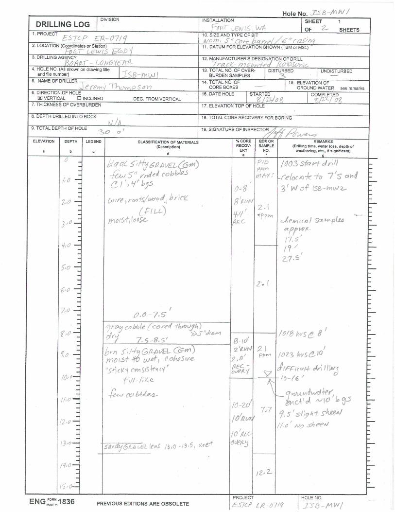


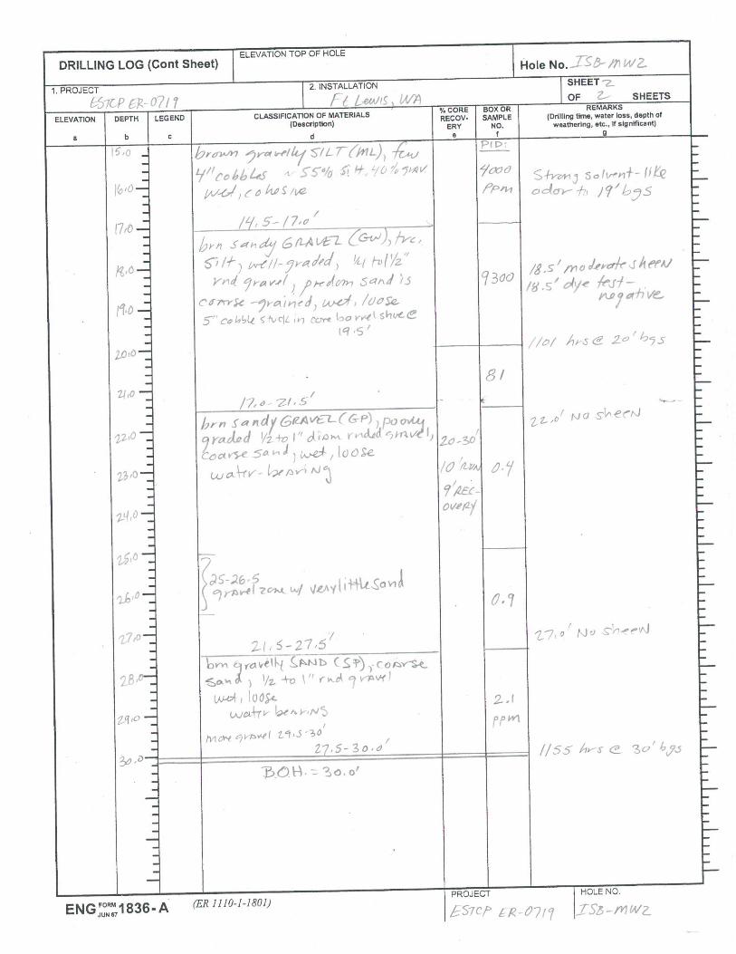

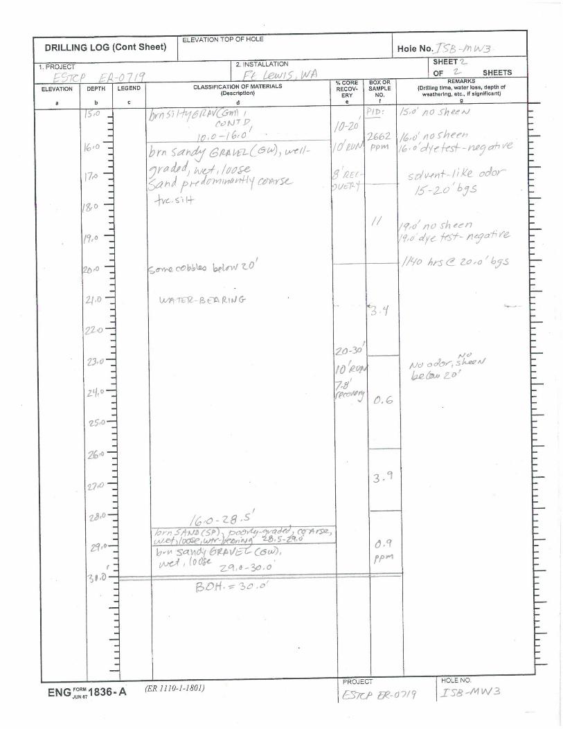


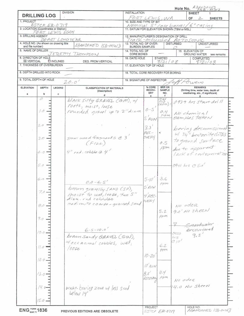
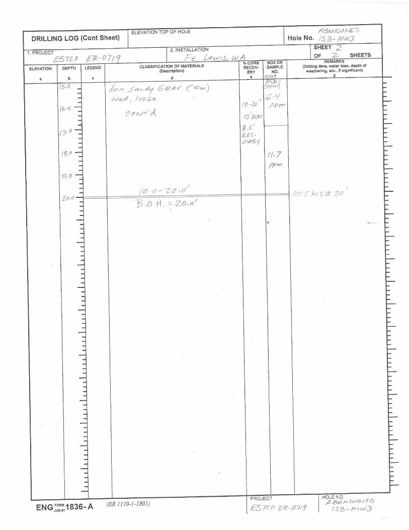
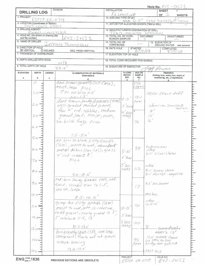
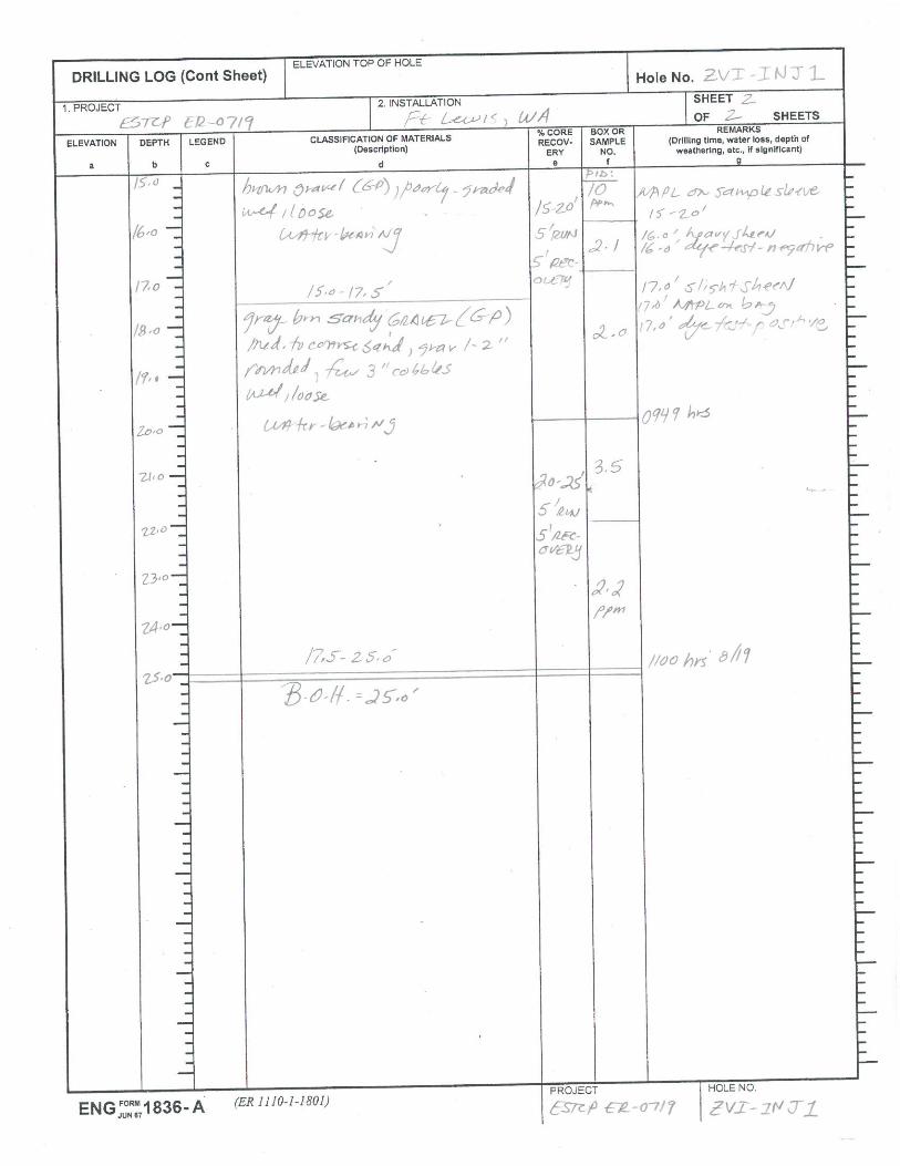

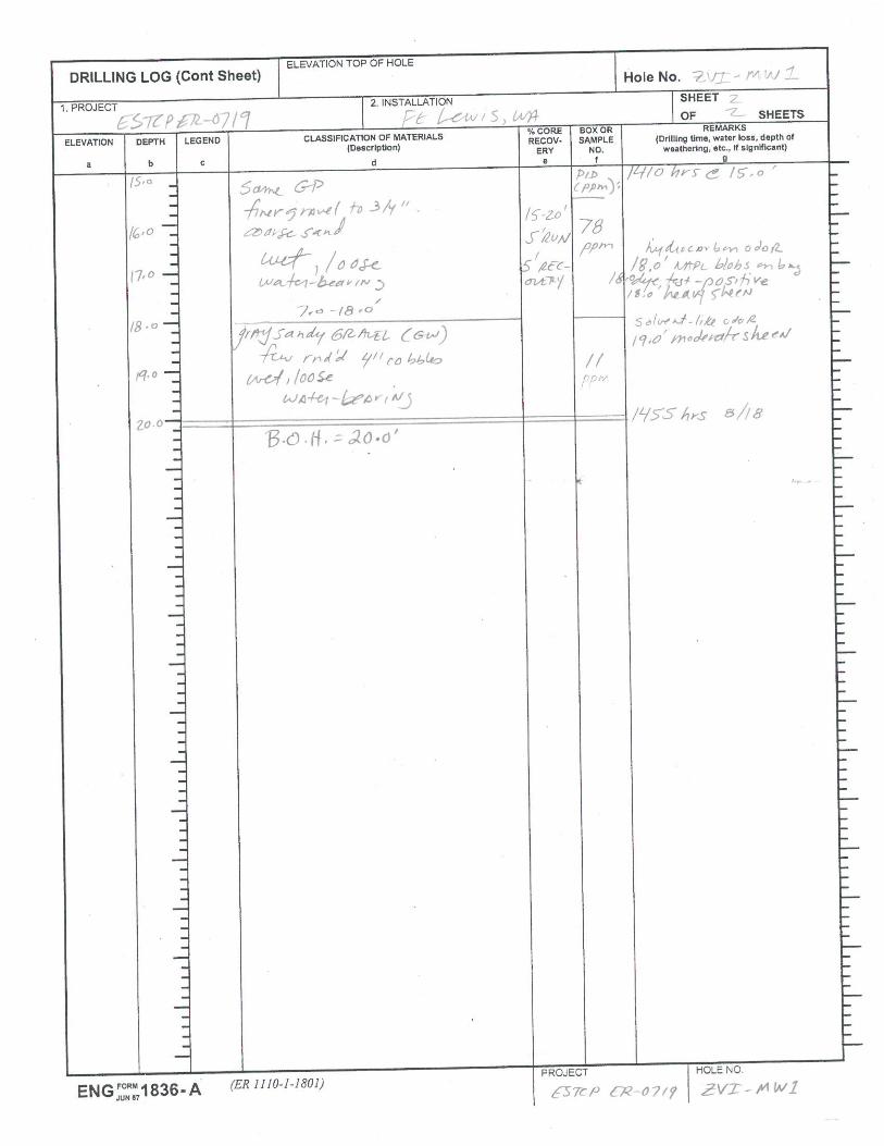

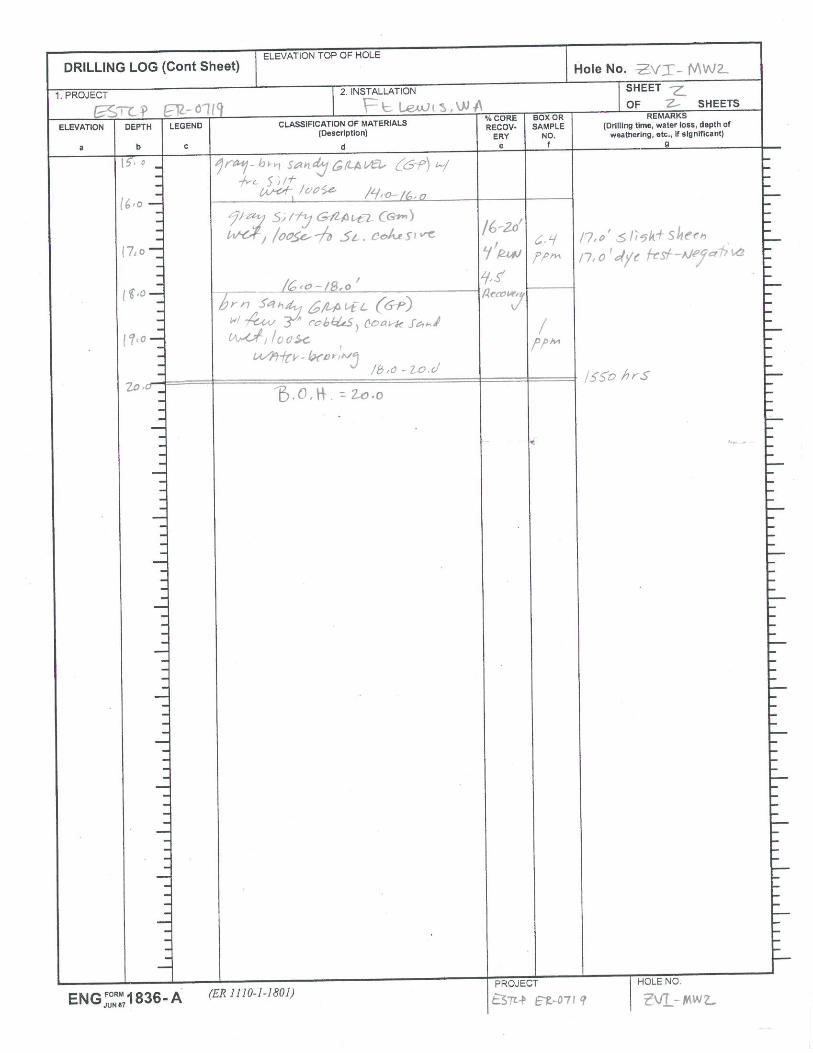

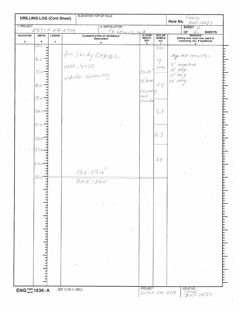

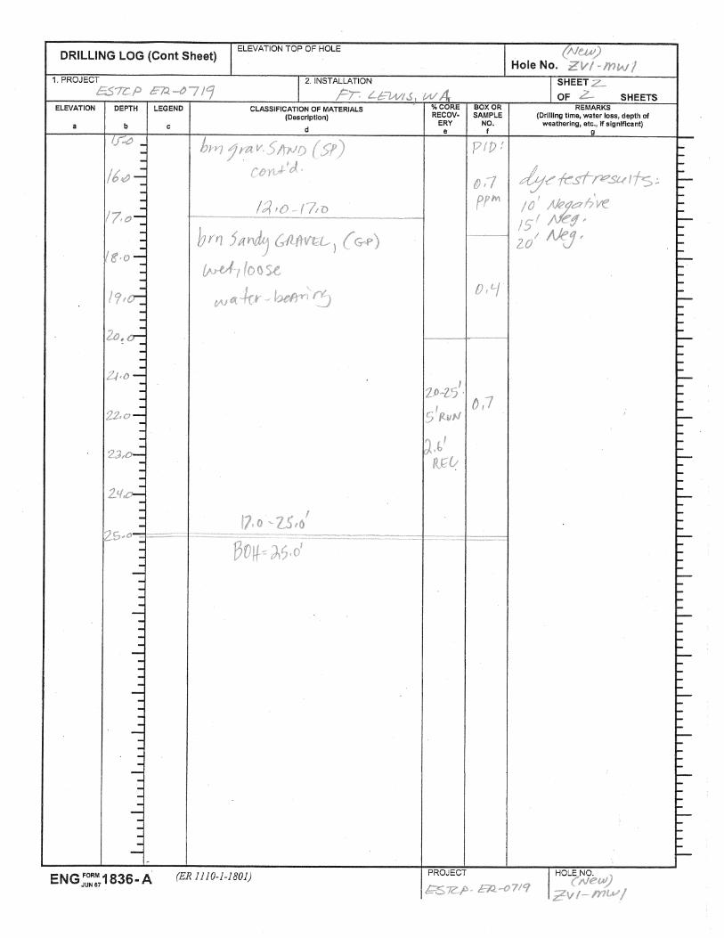


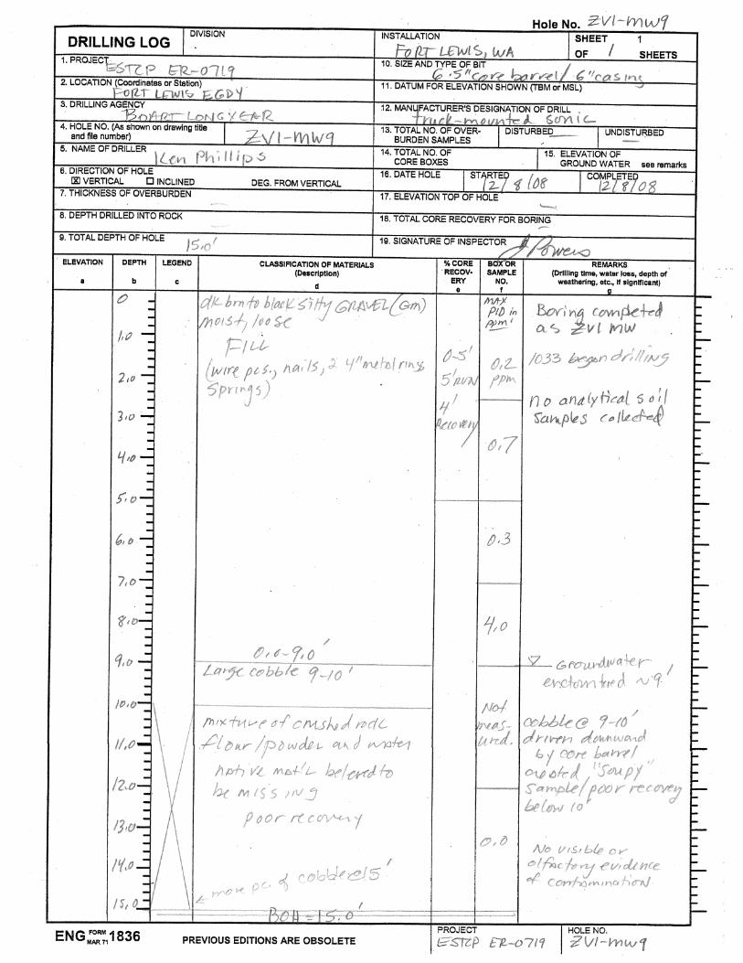
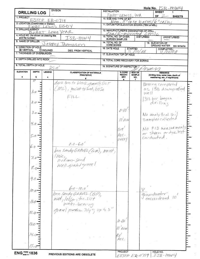


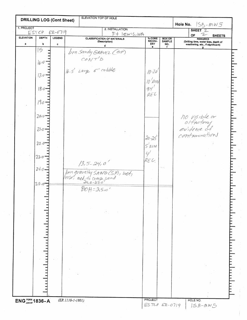

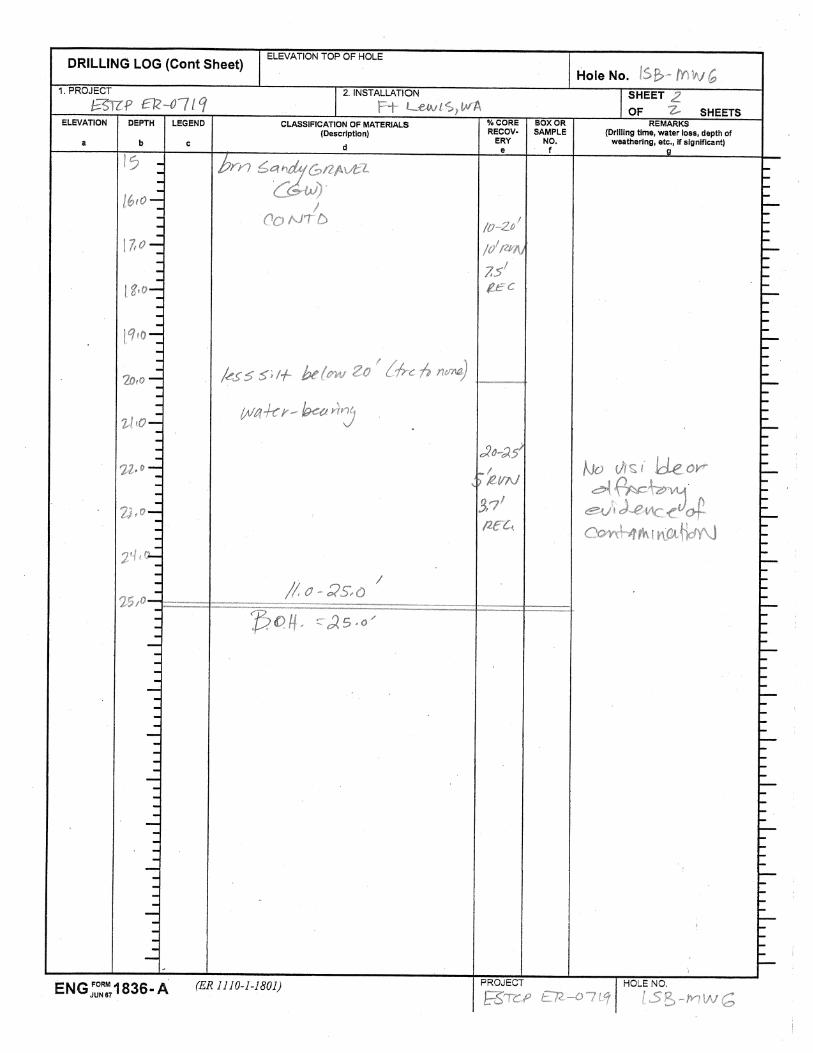
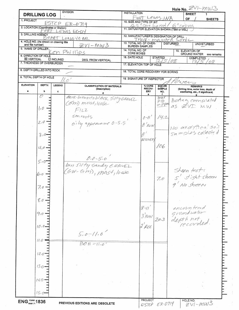

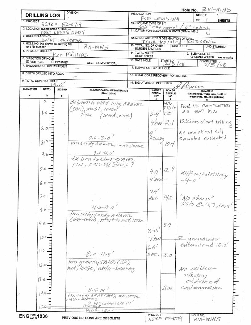
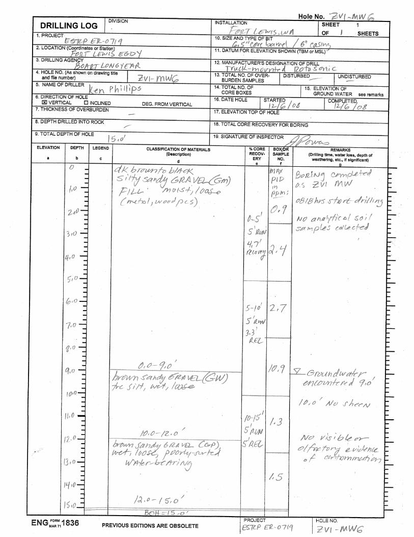
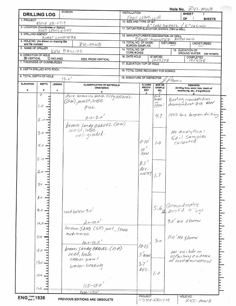


APPENDIX C
LABORATORY TEST REPORT

Bench-Scale Treatability Test Results: Reactivity of Zero-Valent Iron Emplaced by Polymer Solutions
Prepared for: Environmental Security Technology Certification Program
Prepared by: North Wind, Inc.
Pacific Northwest National Laboratory
June 2008
October 2008
NWI-1504-002
Bench-Scale Treatability Test Results: Reactivity to Zero-Valent Iron Emplaced
by Polymer Solutions
October 2008
Prepared for:
SERDP/ESTCP 901 N Stuart St., Suite 303
Arlington, VA 22203
Prepared by: North Wind, Inc. 1425 Higham St.
Idaho Falls, ID 83402
Pacific Northwest National Laboratory P.O. Box 999
Richland, WA 99352
Contract No. ER-0719/PNNL 52036

Bench-Scale Treatability Test Results North Wind, Inc. Zero-Valent Iron Emplaced by Polymer Solutions October 2008
iii
CONTENTS ACRONYMS............................................................................................................................................... iv
1. BACKGROUND................................................................................................................................ 1
2. OBJECTIVES..................................................................................................................................... 3
3. METHODS......................................................................................................................................... 3
4. RESULTS........................................................................................................................................... 5
4.1 Stoichiometry ........................................................................................................................ 5
4.1.1 High ZVI Loading............................................................................................... 5 4.1.2 Low ZVI Loading ............................................................................................... 5
4.2 Dechlorination Rate............................................................................................................... 6
4.2.1 High ZVI Loading............................................................................................... 6 4.2.2 Low ZVI Loading ............................................................................................... 9
5. DISCUSSION RELATIVE TO TEST OBJECTIVES....................................................................... 9
6. REFERENCES................................................................................................................................. 10
TABLES
Table 1. Treatment matrix............................................................................................................................. 4
Table 2. Measured TCE dechlorination extent for low ZVI loading. ........................................................... 5
Table 3. Dechlorination rate and extent in high ZVI loading experiments................................................... 8
FIGURES
Figure 1. Potential TCE transformation reactions with ZVI. The ER-0719 project work is focusing on the reductive elimination pathway. .......................................................................................................... 1
Figure 2. TCE concentration over time in experiments with high initial TCE concentrations (0.16 g TCE added) at 20oC. Note: Concentrations of TCE on the figure were computed from the added TCE mass and the chloride measurements assuming that all of the TCE is in the aqueous phase..... 6
Figure 3. TCE concentration over time in experiments with high initial TCE concentrations (0.16 g TCE added) at 40oC. Note: Concentrations of TCE on the figure were computed from the added TCE mass and the chloride measurements assuming that all of the TCE is in the aqueous phase..... 7
Figure 4. TCE concentration over time in experiments with low initial TCE concentrations (0.016 g TCE added) at 20oC. Note: Concentrations of TCE on the figure were computed from the added TCE mass and the chloride measurements assuming that all of the TCE is in the aqueous phase..... 7
Figure 5. TCE concentration over time in experiments with low initial TCE concentrations (0.016 g TCE added) at 40oC. ....................................................................................................................... 8
Bench-Scale Treatability Test Results North Wind, Inc. Zero-Valent Iron Emplaced by Polymer Solutions October 2008
iv
ACRONYMS
EGDY East Gate Disposal Yard
ESTCP Environmental Security Technology Certification Program
FID/ECD flame ionization detector/electrochemical detector
GC gas chromatograph
NAPL nonaqueous phase liquid
TCE trichloroethene
ZVI zero-valent iron
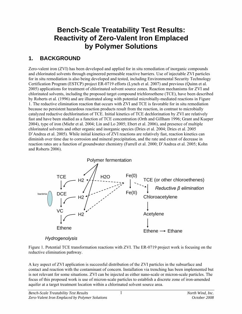
Bench-Scale Treatability Test Results North Wind, Inc. Zero-Valent Iron Emplaced by Polymer Solutions October 2008
1
Bench-Scale Treatability Test Results: Reactivity of Zero-Valent Iron Emplaced
by Polymer Solutions 1. BACKGROUND
Zero-valent iron (ZVI) has been developed and applied for in situ remediation of inorganic compounds and chlorinated solvents through engineered permeable reactive barriers. Use of injectable ZVI particles for in situ remediation is also being developed and tested, including Environmental Security Technology Certification Program (ESTCP) project ER-0719 efforts (Lynch et al. 2007) and previous (Quinn et al. 2005) applications for treatment of chlorinated solvent source zones. Reaction mechanisms for ZVI and chlorinated solvents, including the proposed target compound trichloroethene (TCE), have been described by Roberts et al. (1996) and are illustrated along with potential microbially-mediated reactions in Figure 1. The reductive elimination reaction that occurs with ZVI and TCE is favorable for in situ remediation because no persistent hazardous reaction products result from the reaction, in contrast to microbially catalyzed reductive dechlorination of TCE. Initial kinetics of TCE dechlorination by ZVI are relatively fast and have been studied as a function of TCE concentration (Orth and Gillham 1996; Grant and Kueper 2004), type of iron (Miehr et al. 2004; Lin and Lo 2005; Ebert et al. 2006), and presence of multiple chlorinated solvents and other organic and inorganic species (Dries et al. 2004; Dries et al. 2005 D’Andrea et al. 2005). While initial kinetics of ZVI reactions are relatively fast, reaction kinetics can diminish over time due to corrosion and mineral precipitation, and the rate and extent of decrease in reaction rates are a function of groundwater chemistry (Farrell et al. 2000; D’Andrea et al. 2005; Kohn and Roberts 2006).
TCE
DCE
VC
Ethene
H2
H2
H2
Hydrogenolysis
TCE (or other chloroethenes)
Chloroacetylene
Acetylene
Ethene Ethane
Fe(0)
Fe(II)Reductive β elimination
H2O
Polymer fermentation
bacteria
Figure 1. Potential TCE transformation reactions with ZVI. The ER-0719 project work is focusing on the reductive elimination pathway.
A key aspect of ZVI application is successful distribution of the ZVI particles in the subsurface and contact and reaction with the contaminant of concern. Installation via trenching has been implemented but is not relevant for some situations. ZVI can be injected as either nano-scale or micron-scale particles. The focus of this proposed work is use of micron-scale particles to establish a discrete zone of iron-amended aquifer at a target treatment location within a chlorinated solvent source area.

Bench-Scale Treatability Test Results North Wind, Inc. Zero-Valent Iron Emplaced by Polymer Solutions October 2008
2
Micron-scale ZVI, and not nano-scale ZVI, was selected for the ESTCP field demonstration for the following reasons:
1. Nano-scale ZVI could potentially be extracted through the sampling system and be lost downgradient rather than remain as a reactive zone in the aquifer.
2. Micron-scale ZVI particles have a longer reactive lifetime.
While micron-scale particles are preferred, injection of micron-scale particles is problematic due to the high density of the iron particles, which limits the distance particles can be injected from a well. Research on improved injection strategies for iron particles has been conducted using emulsified oil (Quinn et al. 2005), hydrofracturing of the aquifer (www.GeoSierra.com), use of carrier particles (Schrick et al. 2004), and co-injection of iron with polymers (Cantrell et al. 1997a, b; DOE 2004; Oostrom et al. 2005, 2007). Results from a field test of emulsified ZVI revealed problems with the uniformity of the injection. In addition, it promoted microbial reductive dechlorination as a major reaction process stimulated by the emulsified oil rather than exclusively the reductive elimination reaction from the injected iron (Quinn et al. 2005). At the elevated temperatures required for the field pilot demonstration, significant biological reductive dechlorination is not favored and therefore, emulsified ZVI is not desirable because the effectiveness of the product relies on biological reduction.
Emplacement of ZVI via hydrofracturing has been applied for multiple purposes in the subsurface (www.GeoSierra.com; EPA 1993) but is not suitable for many sites due to the site geology and does not result in a uniform distribution of injected materials around the injection point. Carrier particles (i.e., hydrophilic carbon and poly acrylic acid) have been tested to promote better transport of iron through porous media. However, these tests (Schrick et al. 2004), conducted in small downward-flow columns, have not addressed particle density issues and injection uniformity from an injection well and therefore, are not poised for field testing.
For the thermally-enhanced ZVI field demonstration, the use of shear-thinning polymers to distribute micron-scale ZVI has significant promise in meeting project objectives. These polymers have been shown to promote uniform distribution of ZVI particles in columns and large-scale wedge-shaped flow cells (Cantrell et al. 1997a, b; DOE 2004; Oostrom et al. 2005, 2007). In contrast to the other mechanisms for ZVI injection that rely on encapsulating or carrying the iron particles, the relatively low concentrations of polymer required (fraction of a percent) minimize the amount of organic carbon added to the aquifer. For the ESTCP demonstration, limiting the amended carbon is desired to minimize the biotic reactions in the ZVI test cell making the data interpretation of relative abiotic degradation rates under ambient and heated conditions more straightforward.
The cost benefit of thermally-enhanced processes relies on offsetting the cost of heating by more efficient in situ treatment. Under this condition, it is important to effectively deliver a sufficient amount of reactive ZVI to take advantage of the increased reaction rates at higher temperatures and complete treatment within a short period of time. The delivery method must be suitable for emplacing the ZVI and enabling the abiotic degradation mechanisms to proceed unhindered (i.e., without interference from encapsulation materials). For these reasons, polymer assisted ZVI injection was selected as the most promising injection method for the ESTCP field test. Existing laboratory data provide a good basis for designing an effective injection strategy for the field test. However, the impact of the polymer on the ZVI reactivity needs to be determined to confirm that the polymer does not negatively impact the ability of the emplaced ZVI to degrade contaminants. A key performance metric of the field test will be examining the effectiveness of the treatment in terms of relative degradation rates under ambient and heated condition. Thus, the potential impacts of the polymer on ZVI reactivity needs to be understood in order to more effectively interpret data collected during the field demonstration.
Bench-Scale Treatability Test Results North Wind, Inc. Zero-Valent Iron Emplaced by Polymer Solutions October 2008
3
2. OBJECTIVES
Distribution of ZVI particles for the ESTCP field test using polymer solutions was selected as the most promising technique to meet the needs of the field test (as discussed above). The characteristics of the polymer delivery will enhance the ability to distribute ZVI more uniformly in the target treatment zone compared to other potential delivery methods for micron-scale ZVI. The injection will emplace both ZVI and polymer within the test zone. While the reactivity of ZVI is relatively well known in aqueous media, the impact of the polymer on reactivity has not been measured. The reactivity of ZVI in the polymer was determined to 1) finalize selection of the polymer as the delivery mechanism for the ZVI, 2) determine injection parameters such as the quantity of ZVI/polymer addition, and 3) provide baseline reaction kinetics to assist in field data interpretation.
3. METHODS
Two different experimental methods were employed in evaluating the dechlorination reactivity of ZVI under conditions relevant to the design of the field test. One set of experiments was conducted in serum bottles with Fort Lewis sediment, water or water and SlurryPro, ZVI, and TCE. These experiments included two different initial TCE concentrations and incubation at 20 and 40oC. This experimental method provides for testing of ZVI reactivity under conditions approximating the field site conditions. The maximum laboratory incubation of 40oC is lower than the targeted temperature for the field test (50 to 55oC). However, preliminary laboratory tests at higher incubation temperatures were problematic and consistent results could only be obtained at 40oC or lower. Additionally, while 55oC is the final target temperature for the field test, the likely heating rate of about 1 to 2oC/day will result in a relatively long period of the test when the temperatures are between 12oC (ambient) and 55oC. Site sediments were glacial outwash material obtained from a borehole within the TCE plume about 100 yards downgradient of the East Gate Disposal Yard (EGDY). The other set of experiments was conducted in serum bottles with water or water and SlurryPro, ZVI, and TCE. These experiments included two different initial TCE concentrations, two different ZVI concentrations, and incubation at 20 and 40oC. Chloride concentrations were used as the primary measure of dechlorination. A stoichiometry of 3 moles of chloride per mole of TCE dechlorinated was used to convert chloride concentrations to equivalent TCE concentrations. All treatments were conducted in duplicate and experimental methods included control treatments to monitor for TCE loss and to set baseline chloride levels for comparison to active treatments. The headspace for all treatments was nitrogen gas. The experimental matrix is summarized in Table 1.
Experiments were conducted in a 250-mL serum bottle sealed with VICI Mininert™ valves, a nitrogen headspace, and the specific treatment components defined in Table 1. TCE concentrations were analyzed from headspace samples injected directly to a gas chromatography using Static Headspace Sampling and injected on a Agilent Technologies 6890N gas chromatograph (GC) with a DB-624 column and flame ionization detector/electrochemical detector (FID/ECD) detection. Aqueous chloride samples were analyzed by ion chromatography using a Dionex system with a AS11HC anion exchange column and suppressed conductivity detection.
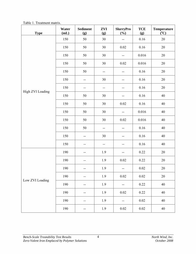
Bench-Scale Treatability Test Results North Wind, Inc. Zero-Valent Iron Emplaced by Polymer Solutions October 2008
4
Table 1. Treatment matrix.
Type Water (mL)
Sediment (g)
ZVI (g)
SlurryPro (%)
TCE (g)
Temperature (oC)
150 50 30 -- 0.16 20
150 50 30 0.02 0.16 20
150 50 30 -- 0.016 20
150 50 30 0.02 0.016 20
150 50 -- -- 0.16 20
150 -- 30 -- 0.16 20
150 -- -- -- 0.16 20
150 50 30 -- 0.16 40
150 50 30 0.02 0.16 40
150 50 30 -- 0.016 40
150 50 30 0.02 0.016 40
150 50 -- -- 0.16 40
150 -- 30 -- 0.16 40
High ZVI Loading
150 -- -- -- 0.16 40
190 -- 1.9 -- 0.22 20
190 -- 1.9 0.02 0.22 20
190 -- 1.9 -- 0.02 20
190 -- 1.9 0.02 0.02 20
190 -- 1.9 -- 0.22 40
190 -- 1.9 0.02 0.22 40
190 -- 1.9 -- 0.02 40
Low ZVI Loading
190 -- 1.9 0.02 0.02 40
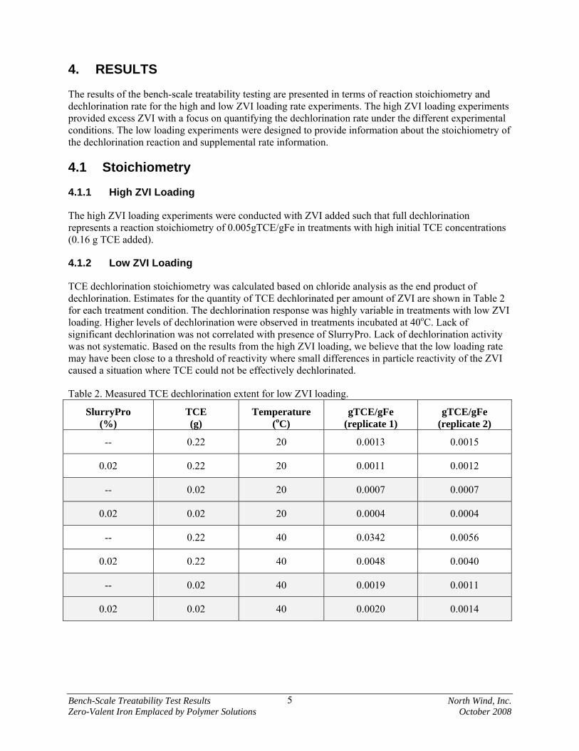
Bench-Scale Treatability Test Results North Wind, Inc. Zero-Valent Iron Emplaced by Polymer Solutions October 2008
5
4. RESULTS
The results of the bench-scale treatability testing are presented in terms of reaction stoichiometry and dechlorination rate for the high and low ZVI loading rate experiments. The high ZVI loading experiments provided excess ZVI with a focus on quantifying the dechlorination rate under the different experimental conditions. The low loading experiments were designed to provide information about the stoichiometry of the dechlorination reaction and supplemental rate information.
4.1 Stoichiometry
4.1.1 High ZVI Loading
The high ZVI loading experiments were conducted with ZVI added such that full dechlorination represents a reaction stoichiometry of 0.005gTCE/gFe in treatments with high initial TCE concentrations (0.16 g TCE added).
4.1.2 Low ZVI Loading
TCE dechlorination stoichiometry was calculated based on chloride analysis as the end product of dechlorination. Estimates for the quantity of TCE dechlorinated per amount of ZVI are shown in Table 2 for each treatment condition. The dechlorination response was highly variable in treatments with low ZVI loading. Higher levels of dechlorination were observed in treatments incubated at 40oC. Lack of significant dechlorination was not correlated with presence of SlurryPro. Lack of dechlorination activity was not systematic. Based on the results from the high ZVI loading, we believe that the low loading rate may have been close to a threshold of reactivity where small differences in particle reactivity of the ZVI caused a situation where TCE could not be effectively dechlorinated.
Table 2. Measured TCE dechlorination extent for low ZVI loading.
SlurryPro (%)
TCE (g)
Temperature (oC)
gTCE/gFe (replicate 1)
gTCE/gFe (replicate 2)
-- 0.22 20 0.0013 0.0015
0.02 0.22 20 0.0011 0.0012
-- 0.02 20 0.0007 0.0007
0.02 0.02 20 0.0004 0.0004
-- 0.22 40 0.0342 0.0056
0.02 0.22 40 0.0048 0.0040
-- 0.02 40 0.0019 0.0011
0.02 0.02 40 0.0020 0.0014

Bench-Scale Treatability Test Results North Wind, Inc. Zero-Valent Iron Emplaced by Polymer Solutions October 2008
6
4.2 Dechlorination Rate
4.2.1 High ZVI Loading
The dechlorination rate in experiments at the high ZVI loading rate was dependent on temperature, TCE concentration, and the presence of site sediment. Figures 2 and 3 illustrate the observed TCE dechlorination in treatments with high initial TCE concentration (0.16 g TCE added) at 20 and 40oC, respectively. Figures 4 and 5 illustrate observed TCE dechlorination in treatments with low initial TCE concentration (0.016 g TCE added) at 20 and 40oC, respectively. In treatments containing site sediments, the dechlorination rates appear to be attenuated compared to the water-only rates. Table 3 shows the dechlorination rate and extent derived for each treatment. Rates are computed as both a pseudo first-order rate coefficient and as a zero-order reaction. Comparing the first-order rate coefficients at the two TCE concentrations that were tested and examining the shape of the TCE concentration profile in Figure 2 demonstrates that the reaction rate is not strictly first order. However, comparing the zero-order rates for the two TCE concentrations that were tested demonstrates there is a concentration dependence to the reaction. Under the field test conditions, the groundwater concentrations will be controlled by the relative rate of reaction to the rate of mass transfer from nonaqueous phase liquid (NAPL) and sorbed phase TCE. The laboratory data will be used for comparison to field data in evaluating the overall processes that occur during the field test.
The zero-order reaction rates in SlurryPro range from about 80 to over 100% of the rates in water. Thus, the impact of SlurryPro on the ZVI reactions is deemed to be minimal. For treatments containing site sediments, reaction rates at 40oC are about 2.5 to 4 times faster than rates at 20oC. As such, the reaction rate is expected to be significantly enhanced by the heating process during the field test.
0
200
400
600
800
1000
1200
0 5 10 15 20 25 30
Time (days)
TCE
con
cent
ratio
n (m
g/L)
sediment and w ater, replicate 1
sediment and w ater, replicate 2
sediment, w ater, and SlurryPro, replicate 1
sediment, w ater, and SlurryPro, replicate 2
w ater, replicate 1
w ater, replicate 2
Figure 2. TCE concentration over time in experiments with high initial TCE concentrations (0.16 g TCE added) at 20oC. Note: Concentrations of TCE on the figure were computed from the added TCE mass and the chloride measurements assuming that all of the TCE is in the aqueous phase.

Bench-Scale Treatability Test Results North Wind, Inc. Zero-Valent Iron Emplaced by Polymer Solutions October 2008
7
0
200
400
600
800
1000
1200
0 5 10 15 20 25 30
Time (days)
TCE
con
cent
ratio
n (m
g/L)
sediment and w ater, replicate 1
sediment and w ater, replicate 2
sediment, w ater, and SlurryPro, replicate 1
sediment, w ater, and SlurryPro, replicate 2
w ater, replicate 1
w ater, replicate 2
Figure 3. TCE concentration over time in experiments with high initial TCE concentrations (0.16 g TCE added) at 40oC. Note: Concentrations of TCE on the figure were computed from the added TCE mass and the chloride measurements assuming that all of the TCE is in the aqueous phase.
0
20
40
60
80
100
120
0 5 10 15 20 25 30
Time (days)
TCE
conc
entr
atio
n (m
g/L)
sediment and w ater, replicate 1
sediment and w ater, replicate 2
sediment, w ater, and SlurryPro, replicate 1
sediment, w ater, and SlurryPro, replicate 2
Figure 4. TCE concentration over time in experiments with low initial TCE concentrations (0.016 g TCE added) at 20oC. Note: Concentrations of TCE on the figure were computed from the added TCE mass and the chloride measurements assuming that all of the TCE is in the aqueous phase.
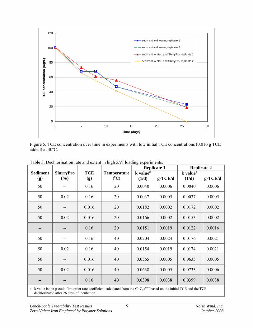
Bench-Scale Treatability Test Results North Wind, Inc. Zero-Valent Iron Emplaced by Polymer Solutions October 2008
8
0
20
40
60
80
100
120
0 5 10 15 20 25 30
Time (days)
TCE
con
cent
ratio
n (m
g/L)
sediment and w ater, replicate 1
sediment and w ater, replicate 2
sediment, w ater, and SlurryPro, replicate 1
sediment, w ater, and SlurryPro, replicate 2
Figure 5. TCE concentration over time in experiments with low initial TCE concentrations (0.016 g TCE added) at 40oC.
Table 3. Dechlorination rate and extent in high ZVI loading experiments. Replicate 1 Replicate 2
Sediment (g)
SlurryPro (%)
TCE (g)
Temperature (oC)
k valuea (1/d) g-TCE/d
k valuea (1/d) g-TCE/d
50 -- 0.16 20 0.0040 0.0006 0.0040 0.0006
50 0.02 0.16 20 0.0037 0.0005 0.0037 0.0005
50 -- 0.016 20 0.0182 0.0002 0.0172 0.0002
50 0.02 0.016 20 0.0166 0.0002 0.0153 0.0002
-- -- 0.16 20 0.0151 0.0019 0.0122 0.0016
50 -- 0.16 40 0.0204 0.0024 0.0176 0.0021
50 0.02 0.16 40 0.0154 0.0019 0.0174 0.0021
50 -- 0.016 40 0.0565 0.0005 0.0635 0.0005
50 0.02 0.016 40 0.0638 0.0005 0.0733 0.0006
-- -- 0.16 40 0.0398 0.0038 0.0399 0.0038
a. k value is the pseudo first order rate coefficient calculated from the C=Coe(-kt) based on the initial TCE and the TCE dechlorinated after 26 days of incubation.
Bench-Scale Treatability Test Results North Wind, Inc. Zero-Valent Iron Emplaced by Polymer Solutions October 2008
9
4.2.2 Low ZVI Loading
Because the dechlorination response was highly variable for low ZVI loading treatments, dechlorination rates were not calculated.
5. DISCUSSION RELATIVE TO TEST OBJECTIVES
The laboratory tests were conducted to 1) finalize selection of the polymer as the delivery mechanism for the ZVI, 2) determine injection parameters (i.e., quantity of ZVI/polymer addition), and 3) provide baseline reaction kinetics to assist in field data interpretation.
Laboratory tests indicate that presence of SlurryPro has only a minor effect on the rate and extent of dechlorination. Thus, delivery of the ZVI using the polymer is viable at the polymer concentrations shown to provide the best ZVI distribution in bench-scale wedge-shaped flow cell tests (Oostrom et al. 2007). Increasing the system temperature further minimizes the impact of the polymer on the dechlorination rate and extent catalyzed by the ZVI.
Data for the stoichiometry (i.e., extent) of dechlorination with ZVI are variable due to the variation in dechlorination response for the low ZVI loading treatments. However, these data, in conjunction with the observed responses at the high ZVI loading rate, provide information to support the injection design for the field test. The average stoichiometry for the low ZVI loading treatments at 40oC (most consistent data) and for the high level of initial TCE was 1.2 g-TCE/100 g-ZVI with a maximum value of 3.4 g-TCE/100 g-ZVI. Using a range from the average to the maximum stoichiometry value, 275 to 800 kg of ZVI would be required to dechlorinate 10 kg of TCE in the field test. The low end of the range of laboratory measured stoichiometry was not used in this estimate (e.g., 20oC and low initial TCE data) because the field test conditions will be primarily for the higher temperature and for high TCE mass loading (source zone). The calculated range of ZVI required for the field test can be delivered to the test zone using a weight percentage of ZVI in the injection fluid that is within the range tested in the previous bench-scale experiments (Oostrom et al. 2007). The ZVI injection concentration and target total ZVI mass will be evaluated based on the site characterization data. The injection design will need to balance:
• Uncertainties in the TCE mass estimate within the target zone,
• Uncertainty in the stoichiometry that will be obtained in the field,
• Material cost,
• Increased potential for injection problems with higher total ZVI mass to be injected, and
• Potential for phased injection, whereby the need for and quantity of a second ZVI injection can be determined based on the response observed from the initial injection (e.g., similar to reinjection procedures for bioremediation and other reagent-based treatments).
The dechlorination response was improved with increased temperature (40oC) in terms of reduced variability in low ZVI loading treatments and the overall rate of dechlorination. It is likely that in the field, dechlorination at ambient temperature (~12oC) will be minimal. However, dechlorination will be stimulated by increasing the temperature to 40oC and higher. The laboratory data provided rate information for comparison to data that will be collected during the field test.

Bench-Scale Treatability Test Results North Wind, Inc. Zero-Valent Iron Emplaced by Polymer Solutions October 2008
10
6. REFERENCES
Cantrell K.J., D.I. Kaplan, and T.J. Gilmore. 1997a. “Injection of colloidal size particles of Fe0 in porous media with shear thinning fluids as a method to emplace a permeable reactive zone.” Land Contamination and Reclamation, 5:253-257.
Cantrell K.J., D.I. Kaplan, and T.J. Gilmore. 1997b. “Injection of colloidal Fe0 particles in sand with shear-thinning fluids.” J. Environ. Eng. 123:786-791.
D’Andrea, P., Kieth, C.K. Lai, P. Kjeldsen, and I.M.C. Lo. 2005. “Effect of groundwater inorganics on the reductive dechlorination of TCE by zero-valent iron.” Water, Air, and Soil Pollution. 162:401-420.
DOE. 2004. “Mending the in situ redox manipulation barrier.” Technical Assistance Project #28 Final Technical Solutions Report, U.S. Department of Energy, Washington, D.C.
Dries, J., L. Bastiaens, D. Springael, S.N. Agathos, and L. Diels. 2004. “Competition for sorption and degradation of chlorinated ethenes in batch zero-valent iron systems.” Environ. Sci. Technol. 38:2879-2884.
Dries, J., L. Bastiaens, D. Springael, S.N .Agathos, and L. Diels. 2005. “Combined removal of chlorinated ethenes and heavy metals by zerovalent iron in batch and continuous flow column systems.” Environ. Sci. Technol. 39:8460-8465.
Ebert, M., R. Kober, A. Parbs, V. Plagentz, D. Schafer, and A. Dahmke. 2006. “Assessing degradation rates of chlorinated ethylenes in column experiments with commercial iron materials used in permeable reactive barriers.” Environ. Sci. Technol. 40:2004-2010
EPA. 1993. “Hydraulic Fracturing Technology: Applications Analysis and Technology Evaluation Report,” EPA/540/-93/505, U.S. Environmental Protection Agency Risk Reduction Engineering Laboratory, Cincinnati, OH.
Farrell, J., Kason, M., Melitas, N., Li, T. 2000. “Investigation of the long-term performance of zero-valent iron for reductive dechlorination of trichloroethylene.” Environ. Sci. Technol. 34:514-521.
Grant, G.P. and B.H. Kueper. 2004. “The influence of high initial concentration aqueous-phase TCE on the performance of iron wall systems.” J. Contam. Hydrology 74:299-312
Kohn, T., and A.L. Roberts. 2006. “The effect of silica on the degradation of organohalides in granular iron columns.” J. Contam. Hydrology 83:70-88
Lin, C.J. and S. Lo. 2005. “Effects of iron surface pretreatment on sorption and reduction kinetics of trichloroethylene in a closed batch system.” Water Research. 39:1037-1046.
Lynch, K., M. Truex, V. Vermeul, T. Powell, T. Macbeth, K. Sorenson. 2007. “Combining Low-Energy Electrical Resistance Heating with Biotic and Abiotic Reactions for Treatment of Chlorinated Solvent DNAPL Source Areas.” ESTCP project ER-0719.
Miehr, R.; P.G. Tratnyek, J.Z. Bandstra, M.M. Scherer, M.J. Alowitz, E.J. Bylaska. 2004. “Diversity of contaminant reduction reactions by zerovalent iron: Role of the reductate.” Environ. Sci. Technol. 38:139-147.

Bench-Scale Treatability Test Results North Wind, Inc. Zero-Valent Iron Emplaced by Polymer Solutions October 2008
11
Oostrom, M, T.W. Wietsma, M.A. Covert, and V.R. Vermeul. 2005. “Experimental Study of Micron-Size Zero-Valent Iron Emplacement in Permeable Porous Media Using Polymer-Enhanced Fluids.” PNNL-15573, Pacific Northwest National Laboratory, Richland, Washington.
Oostrom, M., T.W. Wietsma, M.A. Covert, and V.R. Vermeul. 2007. “Zero-valent iron emplacement in permeable porous media using polymer additions.” Ground Water Monitoring and Remediation. 27: 122-130.
Orth, W.S., Gillham, R.W. 1996. “Dechlorination of trichloroethene in aqueous solution using Fe0.” Environ. Sci. Technol. 30:66-71.
Quinn, J., C. Geiger, C. Clausen, K. Brooks, C. Coon, S. O’Hara, T. Krug, D. Major, W-S. Yoon, A. Gavaskar, and T. Holdsworth. 2005. “Field Demonstration of DNAPL Dehalogenation Using Emulsified Zero-Valent Iron.” Environ. Sci. Technol. 39(5):1309-1318.
Roberts, A.L., L.A. Totten, W.A. Arnold, D.R. Burris, and T.J. Campbell. 1996. “Reductive elimination of chlorinated ethylenes by zero-valent metals.” Environ. Sci. Technol. 30(8): 2654-2659.
Schrick, B., B. W. Hydutsky, J. L. Blough, and T. E. Mallouk. 2004. “Delivery Vehicles for Zerovalent Metal Nanoparticles in Soil and Groundwater.” Chem. Mater. 16:2187-2193.

APPENDIX D
ANALYTICAL DATA

Table 1a. ISB Gore Analytical Results
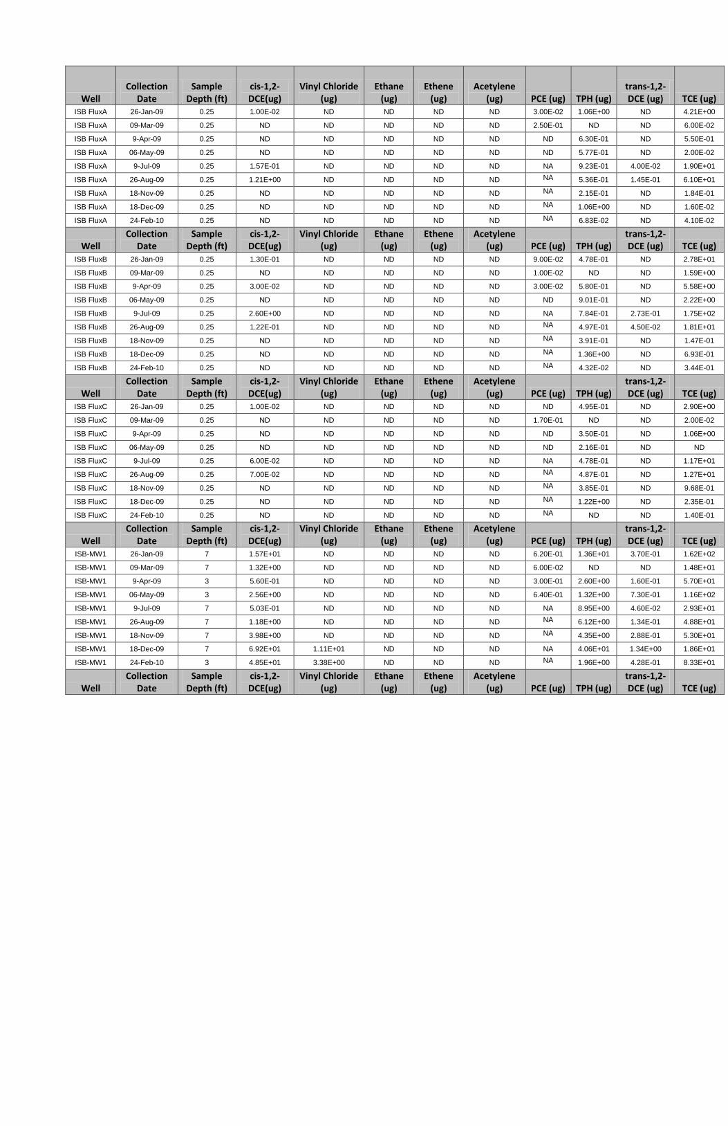
Well Collection
Date Sample
Depth (ft) cis-1,2-DCE(ug)
Vinyl Chloride (ug)
Ethane (ug)
Ethene (ug)
Acetylene (ug) PCE (ug) TPH (ug)
trans-1,2-DCE (ug) TCE (ug)
ISB FluxA 26-Jan-09 0.25 1.00E-02 ND ND ND ND 3.00E-02 1.06E+00 ND 4.21E+00
ISB FluxA 09-Mar-09 0.25 ND ND ND ND ND 2.50E-01 ND ND 6.00E-02
ISB FluxA 9-Apr-09 0.25 ND ND ND ND ND ND 6.30E-01 ND 5.50E-01
ISB FluxA 06-May-09 0.25 ND ND ND ND ND ND 5.77E-01 ND 2.00E-02
ISB FluxA 9-Jul-09 0.25 1.57E-01 ND ND ND ND NA 9.23E-01 4.00E-02 1.90E+01
ISB FluxA 26-Aug-09 0.25 1.21E+00 ND ND ND ND NA 5.36E-01 1.45E-01 6.10E+01
ISB FluxA 18-Nov-09 0.25 ND ND ND ND ND NA 2.15E-01 ND 1.84E-01
ISB FluxA 18-Dec-09 0.25 ND ND ND ND ND NA 1.06E+00 ND 1.60E-02
ISB FluxA 24-Feb-10 0.25 ND ND ND ND ND NA 6.83E-02 ND 4.10E-02
Well Collection
Date Sample
Depth (ft) cis-1,2-DCE(ug)
Vinyl Chloride (ug)
Ethane (ug)
Ethene (ug)
Acetylene (ug) PCE (ug) TPH (ug)
trans-1,2-DCE (ug) TCE (ug)
ISB FluxB 26-Jan-09 0.25 1.30E-01 ND ND ND ND 9.00E-02 4.78E-01 ND 2.78E+01
ISB FluxB 09-Mar-09 0.25 ND ND ND ND ND 1.00E-02 ND ND 1.59E+00
ISB FluxB 9-Apr-09 0.25 3.00E-02 ND ND ND ND 3.00E-02 5.80E-01 ND 5.58E+00
ISB FluxB 06-May-09 0.25 ND ND ND ND ND ND 9.01E-01 ND 2.22E+00
ISB FluxB 9-Jul-09 0.25 2.60E+00 ND ND ND ND NA 7.84E-01 2.73E-01 1.75E+02
ISB FluxB 26-Aug-09 0.25 1.22E-01 ND ND ND ND NA 4.97E-01 4.50E-02 1.81E+01
ISB FluxB 18-Nov-09 0.25 ND ND ND ND ND NA 3.91E-01 ND 1.47E-01
ISB FluxB 18-Dec-09 0.25 ND ND ND ND ND NA 1.36E+00 ND 6.93E-01
ISB FluxB 24-Feb-10 0.25 ND ND ND ND ND NA 4.32E-02 ND 3.44E-01
Well Collection
Date Sample
Depth (ft) cis-1,2-DCE(ug)
Vinyl Chloride (ug)
Ethane (ug)
Ethene (ug)
Acetylene (ug) PCE (ug) TPH (ug)
trans-1,2-DCE (ug) TCE (ug)
ISB FluxC 26-Jan-09 0.25 1.00E-02 ND ND ND ND ND 4.95E-01 ND 2.90E+00
ISB FluxC 09-Mar-09 0.25 ND ND ND ND ND 1.70E-01 ND ND 2.00E-02
ISB FluxC 9-Apr-09 0.25 ND ND ND ND ND ND 3.50E-01 ND 1.06E+00
ISB FluxC 06-May-09 0.25 ND ND ND ND ND ND 2.16E-01 ND ND
ISB FluxC 9-Jul-09 0.25 6.00E-02 ND ND ND ND NA 4.78E-01 ND 1.17E+01
ISB FluxC 26-Aug-09 0.25 7.00E-02 ND ND ND ND NA 4.87E-01 ND 1.27E+01
ISB FluxC 18-Nov-09 0.25 ND ND ND ND ND NA 3.85E-01 ND 9.68E-01
ISB FluxC 18-Dec-09 0.25 ND ND ND ND ND NA 1.22E+00 ND 2.35E-01
ISB FluxC 24-Feb-10 0.25 ND ND ND ND ND NA ND ND 1.40E-01
Well Collection
Date Sample
Depth (ft) cis-1,2-DCE(ug)
Vinyl Chloride (ug)
Ethane (ug)
Ethene (ug)
Acetylene (ug) PCE (ug) TPH (ug)
trans-1,2-DCE (ug) TCE (ug)
ISB-MW1 26-Jan-09 7 1.57E+01 ND ND ND ND 6.20E-01 1.36E+01 3.70E-01 1.62E+02
ISB-MW1 09-Mar-09 7 1.32E+00 ND ND ND ND 6.00E-02 ND ND 1.48E+01
ISB-MW1 9-Apr-09 3 5.60E-01 ND ND ND ND 3.00E-01 2.60E+00 1.60E-01 5.70E+01
ISB-MW1 06-May-09 3 2.56E+00 ND ND ND ND 6.40E-01 1.32E+00 7.30E-01 1.16E+02
ISB-MW1 9-Jul-09 7 5.03E-01 ND ND ND ND NA 8.95E+00 4.60E-02 2.93E+01
ISB-MW1 26-Aug-09 7 1.18E+00 ND ND ND ND NA 6.12E+00 1.34E-01 4.88E+01
ISB-MW1 18-Nov-09 7 3.98E+00 ND ND ND ND NA 4.35E+00 2.88E-01 5.30E+01
ISB-MW1 18-Dec-09 7 6.92E+01 1.11E+01 ND ND ND NA 4.06E+01 1.34E+00 1.86E+01
ISB-MW1 24-Feb-10 3 4.85E+01 3.38E+00 ND ND ND NA 1.96E+00 4.28E-01 8.33E+01
Well Collection
Date Sample
Depth (ft) cis-1,2-DCE(ug)
Vinyl Chloride (ug)
Ethane (ug)
Ethene (ug)
Acetylene (ug) PCE (ug) TPH (ug)
trans-1,2-DCE (ug) TCE (ug)

ISB-MW2 26-Jan-09 7 2.89E+01 ND ND ND ND 2.20E-01 5.32E+00 9.50E-01 4.37E+01
ISB-MW2 09-Mar-09 7 3.89E+00 ND ND ND ND 4.00E-02 ND 1.00E-01 4.88E+00
ISB-MW2 9-Apr-09 3 3.82E+00 ND ND ND ND 1.37E+00 3.30E+00 4.10E-01 1.51E+02
ISB-MW2 06-May-09 7 1.40E+00 ND ND ND ND ND 1.32E+01 ND 4.90E-01
ISB-MW2 9-Jul-09 3 2.27E+00 ND ND ND ND 4.00E-01 7.75E-01 2.50E-01 5.65E+01
ISB-MW2 26-Aug-09 7 4.44E+00 ND ND ND ND NA 3.28E+00 3.93E-01 1.38E+02
ISB-MW2 18-Nov-09 7 9.92E+00 ND ND ND ND NA 3.50E+00 1.02E+00 1.43E+02
ISB-MW2 18-Dec-09 7 2.31E+01 ND ND ND ND NA 4.02E+00 2.55E+00 2.04E+02
ISB-MW2 24-Feb-10 7 8.69E+01 1.12E+01 ND ND ND NA 2.83E+00 2.44E+00 2.77E+01
ISB-MW2 26-Jan-09 3 1.99E+01 ND ND ND ND NA 2.49E+00 2.00E-01 5.38E+01
Well Collection
Date Sample
Depth (ft) cis-1,2-DCE(ug)
Vinyl Chloride (ug)
Ethane (ug)
Ethene (ug)
Acetylene (ug) PCE (ug) TPH (ug)
trans-1,2-DCE (ug) TCE (ug)
ISB-MW3 26-Jan-09 7 2.03E+00 ND ND ND ND 1.90E-01 4.55E+00 1.00E-01 8.24E+01
ISB-MW3 09-Mar-09 7 1.21E+00 ND ND ND ND 3.00E-02
3.00E-02 1.03E+01
ISB-MW3 9-Apr-09 3 4.28E+00 ND ND ND ND 5.90E-01 5.30E-01 5.20E-01 1.83E+02
ISB-MW3 06-May-09 7 2.20E-01 ND ND ND ND ND 4.63E+01 ND 2.10E-01
ISB-MW3 9-Jul-09 3 8.50E-01 ND ND ND ND 8.00E-02 9.61E-01 1.00E-01 3.25E+01
ISB-MW3 26-Aug-09 7 1.45E+00 ND ND ND ND NA 5.49E+00 1.14E-01 8.83E+01
ISB-MW3 18-Nov-09 7 2.23E+00 ND ND ND ND NA 7.46E+00 1.57E-01 6.04E+01
ISB-MW3 18-Dec-09 7 2.07E+01 5.79E-01 ND ND ND NA 3.42E+00 3.63E-01 9.89E+01
ISB-MW3 24-Feb-10 7 1.23E+02 1.00E+02 ND ND ND NA 2.35E+02 2.34E+01 3.38E+00
ISB-MW3 26-Jan-09 3 3.58E+00 ND ND ND ND NA 4.26E-01 5.80E-02 1.76E+01

Table 1b. ZVI Gore Analytical Results
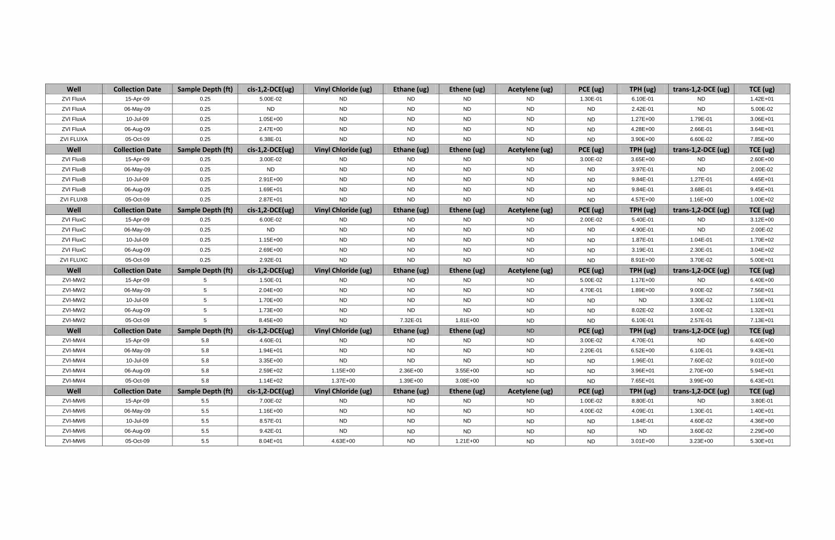
Well Collection Date Sample Depth (ft) cis-1,2-DCE(ug) Vinyl Chloride (ug) Ethane (ug) Ethene (ug) Acetylene (ug) PCE (ug) TPH (ug) trans-1,2-DCE (ug) TCE (ug) ZVI FluxA 15-Apr-09 0.25 5.00E-02 ND ND ND ND 1.30E-01 6.10E-01 ND 1.42E+01
ZVI FluxA 06-May-09 0.25 ND ND ND ND ND ND 2.42E-01 ND 5.00E-02
ZVI FluxA 10-Jul-09 0.25 1.05E+00 ND ND ND ND ND 1.27E+00 1.79E-01 3.06E+01
ZVI FluxA 06-Aug-09 0.25 2.47E+00 ND ND ND ND ND 4.28E+00 2.66E-01 3.64E+01
ZVI FLUXA 05-Oct-09 0.25 6.38E-01 ND ND ND ND ND 3.90E+00 6.60E-02 7.85E+00
Well Collection Date Sample Depth (ft) cis-1,2-DCE(ug) Vinyl Chloride (ug) Ethane (ug) Ethene (ug) Acetylene (ug) PCE (ug) TPH (ug) trans-1,2-DCE (ug) TCE (ug) ZVI FluxB 15-Apr-09 0.25 3.00E-02 ND ND ND ND 3.00E-02 3.65E+00 ND 2.60E+00
ZVI FluxB 06-May-09 0.25 ND ND ND ND ND ND 3.97E-01 ND 2.00E-02
ZVI FluxB 10-Jul-09 0.25 2.91E+00 ND ND ND ND ND 9.84E-01 1.27E-01 4.65E+01
ZVI FluxB 06-Aug-09 0.25 1.69E+01 ND ND ND ND ND 9.84E-01 3.68E-01 9.45E+01
ZVI FLUXB 05-Oct-09 0.25 2.87E+01 ND ND ND ND ND 4.57E+00 1.16E+00 1.00E+02
Well Collection Date Sample Depth (ft) cis-1,2-DCE(ug) Vinyl Chloride (ug) Ethane (ug) Ethene (ug) Acetylene (ug) PCE (ug) TPH (ug) trans-1,2-DCE (ug) TCE (ug) ZVI FluxC 15-Apr-09 0.25 6.00E-02 ND ND ND ND 2.00E-02 5.40E-01 ND 3.12E+00
ZVI FluxC 06-May-09 0.25 ND ND ND ND ND ND 4.90E-01 ND 2.00E-02
ZVI FluxC 10-Jul-09 0.25 1.15E+00 ND ND ND ND ND 1.87E-01 1.04E-01 1.70E+02
ZVI FluxC 06-Aug-09 0.25 2.69E+00 ND ND ND ND ND 3.19E-01 2.30E-01 3.04E+02
ZVI FLUXC 05-Oct-09 0.25 2.92E-01 ND ND ND ND ND 8.91E+00 3.70E-02 5.00E+01
Well Collection Date Sample Depth (ft) cis-1,2-DCE(ug) Vinyl Chloride (ug) Ethane (ug) Ethene (ug) Acetylene (ug) PCE (ug) TPH (ug) trans-1,2-DCE (ug) TCE (ug) ZVI-MW2 15-Apr-09 5 1.50E-01 ND ND ND ND 5.00E-02 1.17E+00 ND 6.40E+00
ZVI-MW2 06-May-09 5 2.04E+00 ND ND ND ND 4.70E-01 1.89E+00 9.00E-02 7.56E+01
ZVI-MW2 10-Jul-09 5 1.70E+00 ND ND ND ND ND ND 3.30E-02 1.10E+01
ZVI-MW2 06-Aug-09 5 1.73E+00 ND ND ND ND ND 8.02E-02 3.00E-02 1.32E+01
ZVI-MW2 05-Oct-09 5 8.45E+00 ND 7.32E-01 1.81E+00 ND ND 6.10E-01 2.57E-01 7.13E+01
Well Collection Date Sample Depth (ft) cis-1,2-DCE(ug) Vinyl Chloride (ug) Ethane (ug) Ethene (ug) ND PCE (ug) TPH (ug) trans-1,2-DCE (ug) TCE (ug) ZVI-MW4 15-Apr-09 5.8 4.60E-01 ND ND ND ND 3.00E-02 4.70E-01 ND 6.40E+00
ZVI-MW4 06-May-09 5.8 1.94E+01 ND ND ND ND 2.20E-01 6.52E+00 6.10E-01 9.43E+01
ZVI-MW4 10-Jul-09 5.8 3.35E+00 ND ND ND ND ND 1.96E-01 7.60E-02 9.01E+00
ZVI-MW4 06-Aug-09 5.8 2.59E+02 1.15E+00 2.36E+00 3.55E+00 ND ND 3.96E+01 2.70E+00 5.94E+01
ZVI-MW4 05-Oct-09 5.8 1.14E+02 1.37E+00 1.39E+00 3.08E+00 ND ND 7.65E+01 3.99E+00 6.43E+01
Well Collection Date Sample Depth (ft) cis-1,2-DCE(ug) Vinyl Chloride (ug) Ethane (ug) Ethene (ug) Acetylene (ug) PCE (ug) TPH (ug) trans-1,2-DCE (ug) TCE (ug) ZVI-MW6 15-Apr-09 5.5 7.00E-02 ND ND ND ND 1.00E-02 8.80E-01 ND 3.80E-01
ZVI-MW6 06-May-09 5.5 1.16E+00 ND ND ND ND 4.00E-02 4.09E-01 1.30E-01 1.40E+01
ZVI-MW6 10-Jul-09 5.5 8.57E-01 ND ND ND ND ND 1.84E-01 4.60E-02 4.36E+00
ZVI-MW6 06-Aug-09 5.5 9.42E-01 ND ND ND ND ND ND 3.60E-02 2.29E+00
ZVI-MW6 05-Oct-09 5.5 8.04E+01 4.63E+00 ND 1.21E+00 ND ND 3.01E+00 3.23E+00 5.30E+01

Table 1. Gore Analytical Results

Well Collection
Date Sample
Depth (ft) cis-1,2-DCE(ug)
Vinyl Chloride (ug)
Ethane (ug)
Ethene (ug)
Acetylene (ug) PCE (ug) TPH (ug)
trans-1,2-DCE (ug) TCE (ug)
ISB FluxA 26-Jan-09 0.25 1.00E-02 ND ND ND ND 3.00E-02 1.06E+00 ND 4.21E+00
ISB FluxA 09-Mar-09 0.25 ND ND ND ND ND 2.50E-01 ND ND 6.00E-02
ISB FluxA 9-Apr-09 0.25 ND ND ND ND ND ND 6.30E-01 ND 5.50E-01
ISB FluxA 06-May-09 0.25 ND ND ND ND ND ND 5.77E-01 ND 2.00E-02
ISB FluxA 9-Jul-09 0.25 1.57E-01 ND ND ND ND NA 9.23E-01 4.00E-02 1.90E+01
ISB FluxA 26-Aug-09 0.25 1.21E+00 ND ND ND ND NA 5.36E-01 1.45E-01 6.10E+01
ISB FluxA 18-Nov-09 0.25 ND ND ND ND ND NA 2.15E-01 ND 1.84E-01
ISB FluxA 18-Dec-09 0.25 ND ND ND ND ND NA 1.06E+00 ND 1.60E-02
ISB FluxA 24-Feb-10 0.25 ND ND ND ND ND NA 6.83E-02 ND 4.10E-02
Well Collection
Date Sample
Depth (ft) cis-1,2-DCE(ug)
Vinyl Chloride (ug)
Ethane (ug)
Ethene (ug)
Acetylene (ug) PCE (ug) TPH (ug)
trans-1,2-DCE (ug) TCE (ug)
ISB FluxB 26-Jan-09 0.25 1.30E-01 ND ND ND ND 9.00E-02 4.78E-01 ND 2.78E+01
ISB FluxB 09-Mar-09 0.25 ND ND ND ND ND 1.00E-02 ND ND 1.59E+00
ISB FluxB 9-Apr-09 0.25 3.00E-02 ND ND ND ND 3.00E-02 5.80E-01 ND 5.58E+00
ISB FluxB 06-May-09 0.25 ND ND ND ND ND ND 9.01E-01 ND 2.22E+00
ISB FluxB 9-Jul-09 0.25 2.60E+00 ND ND ND ND NA 7.84E-01 2.73E-01 1.75E+02
ISB FluxB 26-Aug-09 0.25 1.22E-01 ND ND ND ND NA 4.97E-01 4.50E-02 1.81E+01
ISB FluxB 18-Nov-09 0.25 ND ND ND ND ND NA 3.91E-01 ND 1.47E-01
ISB FluxB 18-Dec-09 0.25 ND ND ND ND ND NA 1.36E+00 ND 6.93E-01
ISB FluxB 24-Feb-10 0.25 ND ND ND ND ND NA 4.32E-02 ND 3.44E-01
Well Collection
Date Sample
Depth (ft) cis-1,2-DCE(ug)
Vinyl Chloride (ug)
Ethane (ug)
Ethene (ug)
Acetylene (ug) PCE (ug) TPH (ug)
trans-1,2-DCE (ug) TCE (ug)
ISB FluxC 26-Jan-09 0.25 1.00E-02 ND ND ND ND ND 4.95E-01 ND 2.90E+00
ISB FluxC 09-Mar-09 0.25 ND ND ND ND ND 1.70E-01 ND ND 2.00E-02
ISB FluxC 9-Apr-09 0.25 ND ND ND ND ND ND 3.50E-01 ND 1.06E+00
ISB FluxC 06-May-09 0.25 ND ND ND ND ND ND 2.16E-01 ND ND
ISB FluxC 9-Jul-09 0.25 6.00E-02 ND ND ND ND NA 4.78E-01 ND 1.17E+01
ISB FluxC 26-Aug-09 0.25 7.00E-02 ND ND ND ND NA 4.87E-01 ND 1.27E+01
ISB FluxC 18-Nov-09 0.25 ND ND ND ND ND NA 3.85E-01 ND 9.68E-01
ISB FluxC 18-Dec-09 0.25 ND ND ND ND ND NA 1.22E+00 ND 2.35E-01
ISB FluxC 24-Feb-10 0.25 ND ND ND ND ND NA ND ND 1.40E-01
Well Collection
Date Sample
Depth (ft) cis-1,2-DCE(ug)
Vinyl Chloride (ug)
Ethane (ug)
Ethene (ug)
Acetylene (ug) PCE (ug) TPH (ug)
trans-1,2-DCE (ug) TCE (ug)
ISB-MW1 26-Jan-09 7 1.57E+01 ND ND ND ND 6.20E-01 1.36E+01 3.70E-01 1.62E+02
ISB-MW1 09-Mar-09 7 1.32E+00 ND ND ND ND 6.00E-02 ND ND 1.48E+01
ISB-MW1 9-Apr-09 3 5.60E-01 ND ND ND ND 3.00E-01 2.60E+00 1.60E-01 5.70E+01
ISB-MW1 06-May-09 3 2.56E+00 ND ND ND ND 6.40E-01 1.32E+00 7.30E-01 1.16E+02
ISB-MW1 9-Jul-09 7 5.03E-01 ND ND ND ND NA 8.95E+00 4.60E-02 2.93E+01
ISB-MW1 26-Aug-09 7 1.18E+00 ND ND ND ND NA 6.12E+00 1.34E-01 4.88E+01
ISB-MW1 18-Nov-09 7 3.98E+00 ND ND ND ND NA 4.35E+00 2.88E-01 5.30E+01
ISB-MW1 18-Dec-09 7 6.92E+01 1.11E+01 ND ND ND NA 4.06E+01 1.34E+00 1.86E+01

ISB-MW1 24-Feb-10 3 4.85E+01 3.38E+00 ND ND ND NA 1.96E+00 4.28E-01 8.33E+01
Well Collection
Date Sample
Depth (ft) cis-1,2-DCE(ug)
Vinyl Chloride (ug)
Ethane (ug)
Ethene (ug)
Acetylene (ug) PCE (ug) TPH (ug)
trans-1,2-DCE (ug) TCE (ug)
ISB-MW2 26-Jan-09 7 2.89E+01 ND ND ND ND 2.20E-01 5.32E+00 9.50E-01 4.37E+01
ISB-MW2 09-Mar-09 7 3.89E+00 ND ND ND ND 4.00E-02 ND 1.00E-01 4.88E+00
ISB-MW2 9-Apr-09 3 3.82E+00 ND ND ND ND 1.37E+00 3.30E+00 4.10E-01 1.51E+02
ISB-MW2 06-May-09 7 1.40E+00 ND ND ND ND ND 1.32E+01 ND 4.90E-01
ISB-MW2 9-Jul-09 3 2.27E+00 ND ND ND ND 4.00E-01 7.75E-01 2.50E-01 5.65E+01
ISB-MW2 26-Aug-09 7 4.44E+00 ND ND ND ND NA 3.28E+00 3.93E-01 1.38E+02
ISB-MW2 18-Nov-09 7 9.92E+00 ND ND ND ND NA 3.50E+00 1.02E+00 1.43E+02
ISB-MW2 18-Dec-09 7 2.31E+01 ND ND ND ND NA 4.02E+00 2.55E+00 2.04E+02
ISB-MW2 24-Feb-10 7 8.69E+01 1.12E+01 ND ND ND NA 2.83E+00 2.44E+00 2.77E+01
ISB-MW2 26-Jan-09 3 1.99E+01 ND ND ND ND NA 2.49E+00 2.00E-01 5.38E+01
Well Collection
Date Sample
Depth (ft) cis-1,2-DCE(ug)
Vinyl Chloride (ug)
Ethane (ug)
Ethene (ug)
Acetylene (ug) PCE (ug) TPH (ug)
trans-1,2-DCE (ug) TCE (ug)
ISB-MW3 26-Jan-09 7 2.03E+00 ND ND ND ND 1.90E-01 4.55E+00 1.00E-01 8.24E+01
ISB-MW3 09-Mar-09 7 1.21E+00 ND ND ND ND 3.00E-02
3.00E-02 1.03E+01
ISB-MW3 9-Apr-09 3 4.28E+00 ND ND ND ND 5.90E-01 5.30E-01 5.20E-01 1.83E+02
ISB-MW3 06-May-09 7 2.20E-01 ND ND ND ND ND 4.63E+01 ND 2.10E-01
ISB-MW3 9-Jul-09 3 8.50E-01 ND ND ND ND 8.00E-02 9.61E-01 1.00E-01 3.25E+01
ISB-MW3 26-Aug-09 7 1.45E+00 ND ND ND ND NA 5.49E+00 1.14E-01 8.83E+01
ISB-MW3 18-Nov-09 7 2.23E+00 ND ND ND ND NA 7.46E+00 1.57E-01 6.04E+01
ISB-MW3 18-Dec-09 7 2.07E+01 5.79E-01 ND ND ND NA 3.42E+00 3.63E-01 9.89E+01
ISB-MW3 24-Feb-10 7 1.23E+02 1.00E+02 ND ND ND NA 2.35E+02 2.34E+01 3.38E+00
ISB-MW3 26-Jan-09 3 3.58E+00 ND ND ND ND NA 4.26E-01 5.80E-02 1.76E+01
Table 1. ZVI GORE Results
Well Collection
Date Sample
Depth (ft) cis-1,2-DCE(ug)
Vinyl Chloride (ug)
Ethane (ug)
Ethene (ug)
Acetylene (ug) PCE (ug) TPH (ug)
trans-1,2-DCE (ug) TCE (ug)
ZVI FluxA 15-Apr-09 0.25 5.00E-02 ND ND ND ND 1.30E-01 6.10E-01 ND 1.42E+01
ZVI FluxA 06-May-09 0.25 ND ND ND ND ND ND 2.42E-01 ND 5.00E-02
ZVI FluxA 10-Jul-09 0.25 1.05E+00 ND ND ND ND ND 1.27E+00 1.79E-01 3.06E+01
ZVI FluxA 06-Aug-09 0.25 2.47E+00 ND ND ND ND ND 4.28E+00 2.66E-01 3.64E+01
ZVI FLUXA 05-Oct-09 0.25 6.38E-01 ND ND ND ND ND 3.90E+00 6.60E-02 7.85E+00
Well Collection
Date Sample
Depth (ft) cis-1,2-DCE(ug)
Vinyl Chloride (ug)
Ethane (ug)
Ethene (ug)
Acetylene (ug) PCE (ug) TPH (ug)
trans-1,2-DCE (ug) TCE (ug)
ZVI FluxB 15-Apr-09 0.25 3.00E-02 ND ND ND ND 3.00E-02 3.65E+00 ND 2.60E+00
ZVI FluxB 06-May-09 0.25 ND ND ND ND ND ND 3.97E-01 ND 2.00E-02
ZVI FluxB 10-Jul-09 0.25 2.91E+00 ND ND ND ND ND 9.84E-01 1.27E-01 4.65E+01
ZVI FluxB 06-Aug-09 0.25 1.69E+01 ND ND ND ND ND 9.84E-01 3.68E-01 9.45E+01
ZVI FLUXB 05-Oct-09 0.25 2.87E+01 ND ND ND ND ND 4.57E+00 1.16E+00 1.00E+02
Well Collection
Date Sample
Depth (ft) cis-1,2-DCE(ug)
Vinyl Chloride (ug)
Ethane (ug)
Ethene (ug)
Acetylene (ug) PCE (ug) TPH (ug)
trans-1,2-DCE (ug) TCE (ug)

ZVI FluxC 15-Apr-09 0.25 6.00E-02 ND ND ND ND 2.00E-02 5.40E-01 ND 3.12E+00
ZVI FluxC 06-May-09 0.25 ND ND ND ND ND ND 4.90E-01 ND 2.00E-02
ZVI FluxC 10-Jul-09 0.25 1.15E+00 ND ND ND ND ND 1.87E-01 1.04E-01 1.70E+02
ZVI FluxC 06-Aug-09 0.25 2.69E+00 ND ND ND ND ND 3.19E-01 2.30E-01 3.04E+02
ZVI FLUXC 05-Oct-09 0.25 2.92E-01 ND ND ND ND ND 8.91E+00 3.70E-02 5.00E+01
Well Collection
Date Sample
Depth (ft) cis-1,2-DCE(ug)
Vinyl Chloride (ug)
Ethane (ug)
Ethene (ug)
Acetylene (ug) PCE (ug) TPH (ug)
trans-1,2-DCE (ug) TCE (ug)
ZVI-MW2 15-Apr-09 5 1.50E-01 ND ND ND ND 5.00E-02 1.17E+00 ND 6.40E+00
ZVI-MW2 06-May-09 5 2.04E+00 ND ND ND ND 4.70E-01 1.89E+00 9.00E-02 7.56E+01
ZVI-MW2 10-Jul-09 5 1.70E+00 ND ND ND ND ND ND 3.30E-02 1.10E+01
ZVI-MW2 06-Aug-09 5 1.73E+00 ND ND ND ND ND 8.02E-02 3.00E-02 1.32E+01
ZVI-MW2 05-Oct-09 5 8.45E+00 ND 7.32E-01 1.81E+00 ND ND 6.10E-01 2.57E-01 7.13E+01
Well Collection
Date Sample
Depth (ft) cis-1,2-DCE(ug)
Vinyl Chloride (ug)
Ethane (ug)
Ethene (ug)
ND PCE (ug) TPH (ug)
trans-1,2-DCE (ug) TCE (ug)
ZVI-MW4 15-Apr-09 5.8 4.60E-01 ND ND ND ND 3.00E-02 4.70E-01 ND 6.40E+00
ZVI-MW4 06-May-09 5.8 1.94E+01 ND ND ND ND 2.20E-01 6.52E+00 6.10E-01 9.43E+01
ZVI-MW4 10-Jul-09 5.8 3.35E+00 ND ND ND ND ND 1.96E-01 7.60E-02 9.01E+00
ZVI-MW4 06-Aug-09 5.8 2.59E+02 1.15E+00 2.36E+00 3.55E+00 ND ND 3.96E+01 2.70E+00 5.94E+01
ZVI-MW4 05-Oct-09 5.8 1.14E+02 1.37E+00 1.39E+00 3.08E+00 ND ND 7.65E+01 3.99E+00 6.43E+01
Well Collection
Date Sample
Depth (ft) cis-1,2-DCE(ug)
Vinyl Chloride (ug)
Ethane (ug)
Ethene (ug)
Acetylene (ug) PCE (ug) TPH (ug)
trans-1,2-DCE (ug) TCE (ug)
ZVI-MW6 15-Apr-09 5.5 7.00E-02 ND ND ND ND 1.00E-02 8.80E-01 ND 3.80E-01
ZVI-MW6 06-May-09 5.5 1.16E+00 ND ND ND ND 4.00E-02 4.09E-01 1.30E-01 1.40E+01
ZVI-MW6 10-Jul-09 5.5 8.57E-01 ND ND ND ND ND 1.84E-01 4.60E-02 4.36E+00
ZVI-MW6 06-Aug-09 5.5 9.42E-01 ND ND ND ND ND ND 3.60E-02 2.29E+00
ZVI-MW6 05-Oct-09 5.5 8.04E+01 4.63E+00 ND 1.21E+00 ND ND 3.01E+00 3.23E+00 5.30E+01

Table 2. ISB and ZVI Soil Gas VOC Summa Results

ISB MW1
Date Depth (ft bgs)
Temp (C) PCE (ug/L)
TCE (ug/L)
cisDCE (ug/L)
transDCE (ug/L)
VC (ug/L)
27-Jan-09 7 10.11 ND 36.20814 1.836221 ND ND
09-Mar-09 7 9.34 ND 22.69177 1.715688 ND ND
10-Apr-09 3 9.57 0.628997 73.68825 1.0453 0.305228 ND
27-Aug-09 7 14.3 0.773309 111.5011 1.644959 0.324879 ND
27-Jan-10 7 23.2 ND 4.812786 4.387783 0.039889 0.138789
23-Feb-10 3 9 0.33662 90.87646 46.08611 0.255568 3.77932
24-Mar-10 3 11.9 ND 118.0619 11.19696 ND ND
20-Apr-10 3 14.1 ND 145.0523 11.52273 ND ND
ISB MW2
Date Depth (ft bgs)
Temp (C) PCE (ug/L)
TCE (ug/L)
cisDCE (ug/L)
transDCE (ug/L)
VC (ug/L)
27-Jan-09 7 9.92 ND 7.925846 2.046255 ND ND
09-Mar-09 7 9.28 ND 20.99435 1.590487 ND ND
10-Apr-09 3 10.43 1.068903 101.7205 2.667852 0.396009 ND
27-Aug-09 7 15.7 1.679042 260.7576 6.547945 0.572945 ND
20-Nov-09 7 28.1 ND 9.575399 82.40426 ND 1.264179
27-Jan-10 7 21.9 ND 70.60886 35.25693 ND ND
23-Feb-10 3 8.3 0.861594 136.6537 28.56045 ND ND
24-Mar-10 3 12 ND 140.5006 31.50632 ND ND
20-Apr-10 3 13.1 ND 100.7717 18.99633 ND ND
ISB MW3
Date Depth (ft bgs)
Temp (C) PCE (ug/L)
TCE (ug/L)
cisDCE (ug/L)
transDCE (ug/L)
VC (ug/L)
27-Jan-09 7 9.52 ND 17.00799 0.313645 ND ND
09-Mar-09 7 9.18 0.2362 24.40748 3.098362 0.062805 ND
10-Apr-09 3 9.4 0.39336 96.41954 1.882672 0.305411 ND
27-Aug-09 7 19.6 ND 186.1202 2.180491 ND ND
20-Nov-09 7 21.5 ND ND 521.5481 ND 51.69985
27-Jan-10 7 13.1 ND 10.07717 4.542601 ND 0.127721
23-Feb-10 3 8.3 0.531316 96.79638 13.02021 0.117602 ND
24-Mar-10 3 12.6 ND 48.79153 153.064 ND 19.99129
20-Apr-10 3 12.5 ND 17.39158 57.93636 0.869045 ND
ZVI MW2
Date Depth (ft bgs)
Temp (C) PCE (ug/L)
TCE (ug/L)
cisDCE (ug/L)
transDCE (ug/L)
VC (ug/L)
09-Apr-09 5.5 9.78 ND 1472.671 31.75353 ND ND
28-May-09 5.5 11.89
ND 1405.548 111.9735
ND ND
10-Jul-09 5.5 25.6 20.96894 3969.495 435.2534 ND ND
24-Jul-09 5.5 30.1 32.65261 4174.82 662.6826 ND ND
05-Aug-09 5.5 35.5 37.97382 4880.598 842.5852 ND ND
20-Aug-09 5.5 36.8 ND 5687.383 610.2191 ND ND

10-Sep-09 5.5 35.9 ND 3889.054 328.9479 ND ND
16-Oct-09 5.5 31.2 ND 2948.67 504.9257 ND ND
12-Nov-09 5.5 25.6 ND 1984.747 474.8219 ND ND
24-Mar-10 5.5 20 ND 1366.663 564.5411 ND ND
ZVI MW4
Date Depth (ft bgs)
Temp (C) PCE (ug/L)
TCE (ug/L)
cisDCE (ug/L)
transDCE (ug/L)
VC (ug/L)
09-Apr-09 5.5 9.51 ND 1700.859 79.45966 ND ND
28-May-09 5.5 12.2
ND 1404.021 745.6793 6.213994
ND
10-Jul-09 5.5 28.7 14.05888 3928.728 1879.782 20.75593 ND
24-Jul-09 5.5 33.2 ND 2458.62 4244.556 57.8803 24.11679
05-Aug-09 5.5 39.6 ND 2715.751 6047.559 52.91614 ND
20-Aug-09 5.5 40.6 ND 970.4682 1130.303 ND ND
10-Sep-09 5.5 41.4 ND 917.0526 2555.505 ND ND
16-Oct-09 5.5 36.4 ND 776.5544 2673.158 ND ND
12-Nov-09 5.5 28.6 ND 525.7743 1488.654 ND ND
24-Mar-10 5.5 23.5 ND 1188.474 107591.2 ND ND
ZVI MW5
Date Depth (ft bgs)
Temp (C) PCE (ug/L)
TCE (ug/L)
cisDCE (ug/L)
transDCE (ug/L)
VC (ug/L)
09-Apr-09 5.5 9.4 ND 1588.087 54.3883 ND ND
28-May-09 5.5 12.07
ND 955.1694 99.46922
ND ND
10-Jul-09 5.5 28.7 ND 5149.819 1018.215 10.57377 ND
24-Jul-09 5.5 33.2 ND 5231.107 2238.038 33.18471 ND
05-Aug-09 5.5 39.6 ND 4970.337 2985.982 41.57697 ND
20-Aug-09 5.5 40.6 ND 9193.909 2938.788 ND ND
10-Sep-09 5.5 41.4 ND 6113.684 1465.657 ND ND
16-Oct-09 5.5 36.4 ND 2381.434 763.7595 ND ND
12-Nov-09 5.5 28.6 ND 1433.93 54.84515 ND ND
24-Mar-10 5.5 23.5 ND 410.5638 1753.338 ND ND
ZVI MW6
Date Depth (ft bgs)
Temp (C) PCE (ug/L)
TCE (ug/L)
cisDCE (ug/L)
transDCE (ug/L)
VC (ug/L)
09-Apr-09 5.5 8.81 1.146714 181.8754 4.19247 1.383515 0.007023
28-May-09 5.5 12.34
ND 162.7866 7.867199 0.910939
ND
10-Jul-09 5.5 28.7 ND 584.0001 101.8215 2.075593 ND
24-Jul-09 5.5 33.2 ND 680.0439 331.8471 5.016293 ND
05-Aug-09 5.5 39.6 ND 871.0901 491.3641 11.71715 ND
20-Aug-09 5.5 40.6 4.444142 970.4682 565.1516 10.92626 ND
10-Sep-09 5.5 41.4 ND 815.1579 450.9714 7.51619 ND
16-Oct-09 5.5 36.4 ND 264.0285 240.5842 ND ND
12-Nov-09 5.5 28.6 ND 122.1496 168.4529 ND ND
24-Mar-10 5.5 23.5 ND 59.42371 75.71234 ND ND

ZVI MW7
Date Depth (ft bgs)
Temp (C) PCE (ug/L)
TCE (ug/L)
cisDCE (ug/L)
transDCE (ug/L)
VC (ug/L)
09-Apr-09 5.5 9.16 2.934811 368.9764 6.699635 0.795582 ND
28-May-09 5.5 11.22
ND 225.4175 5.819715
ND ND
10-Jul-09 5.5 23.7 ND 647.8219 7.167916 ND ND
24-Jul-09 5.5 28.8 ND 175.142 ND ND ND
05-Aug-09 5.5 34.6 ND 67.69502 1.72851 ND ND
20-Aug-09 5.5 35.9 1.307747 191.86 3.21298 ND ND
10-Sep-09 5.5 33.6 0.988165 130.6071 3.314144 ND ND
16-Oct-09 5.5 30.6 ND 147.7247 4.280888 ND ND
12-Nov-09 5.5 25.1 ND 123.583 2.576264 ND ND
24-Mar-10 5.5 18.7 ND 219.6402 6.480637 ND ND
Table 1. Soil Gas Dissolved Gases Summa Results
ISB MW1
Date Depth (ft bgs)
Temp (C) Methane (ug/L)
Ethane (ug/L) Ethene (ug/L)
Acetylene (ug/L)
27-Jan-09 7 10.11 ND ND ND ND
09-Mar-09 7 9.34 ND ND ND ND
10-Apr-09 3 9.57 2.075513 ND ND ND
27-Aug-09 7 14.3 3.674449 ND ND ND
27-Jan-10 7 23.2 21.7806 ND ND ND
23-Feb-10 3 9 14557.94 ND ND ND
24-Mar-10 3 11.9 ND ND ND ND
20-Apr-10 3 14.1 4.698398 ND ND ND
ISB MW2
Date Depth (ft bgs)
Temp (C) Methane (ug/L)
Ethane (ug/L) Ethene (ug/L)
Acetylene (ug/L)
27-Jan-09 7 9.92 ND ND ND ND
09-Mar-09 7 9.28 ND ND ND ND
10-Apr-09 3 10.43 2.276141 ND ND ND
27-Aug-09 7 15.7 4.604657 ND ND ND
20-Nov-09 7 28.1 162.3206 ND ND ND
27-Jan-10 7 21.9 5.502287 ND ND ND
23-Feb-10 3 8.3 ND ND ND ND
24-Mar-10 3 12 ND ND ND ND
20-Apr-10 3 13.1 1.913257 ND ND ND
ISB MW3
Date Depth (ft bgs)
Temp (C) Methane (ug/L)
Ethane (ug/L) Ethene (ug/L)
Acetylene (ug/L)
27-Jan-09 7 9.52 ND ND ND ND
09-Mar-09 7 9.18 ND ND ND ND
10-Apr-09 3 9.4 1.730635 ND ND ND
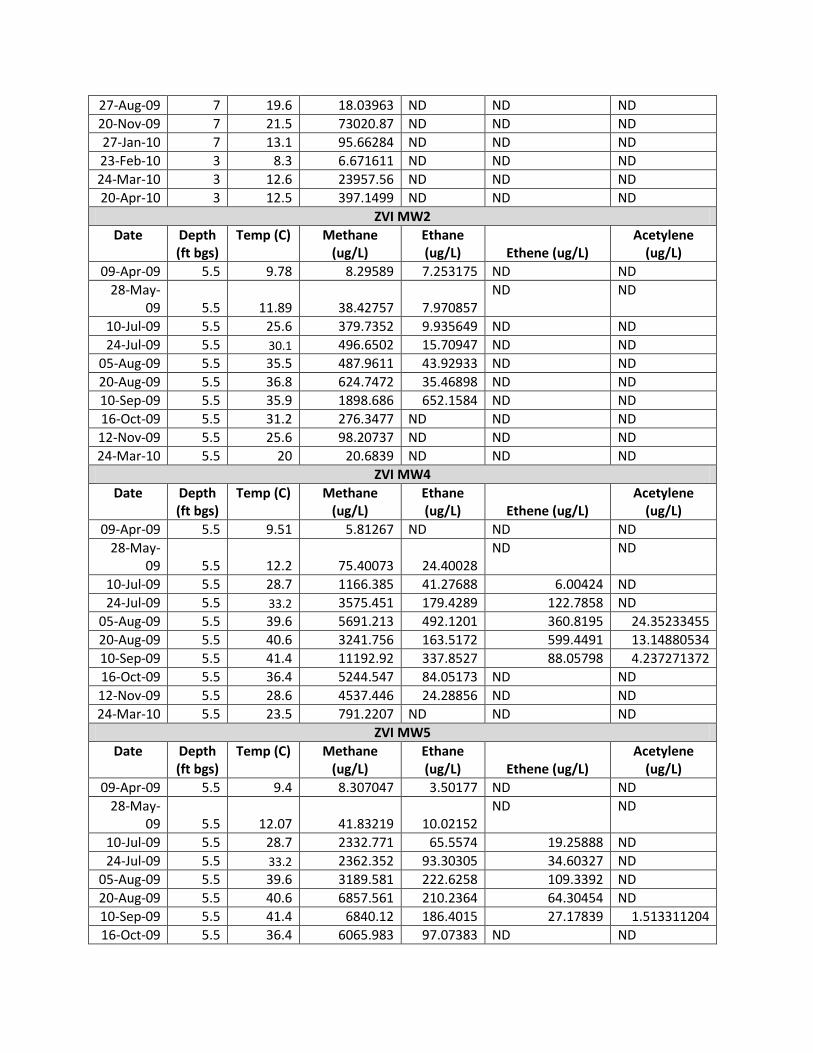
27-Aug-09 7 19.6 18.03963 ND ND ND
20-Nov-09 7 21.5 73020.87 ND ND ND
27-Jan-10 7 13.1 95.66284 ND ND ND
23-Feb-10 3 8.3 6.671611 ND ND ND
24-Mar-10 3 12.6 23957.56 ND ND ND
20-Apr-10 3 12.5 397.1499 ND ND ND
ZVI MW2
Date Depth (ft bgs)
Temp (C) Methane (ug/L)
Ethane (ug/L) Ethene (ug/L)
Acetylene (ug/L)
09-Apr-09 5.5 9.78 8.29589 7.253175 ND ND
28-May-09 5.5 11.89 38.42757 7.970857
ND ND
10-Jul-09 5.5 25.6 379.7352 9.935649 ND ND
24-Jul-09 5.5 30.1 496.6502 15.70947 ND ND
05-Aug-09 5.5 35.5 487.9611 43.92933 ND ND
20-Aug-09 5.5 36.8 624.7472 35.46898 ND ND
10-Sep-09 5.5 35.9 1898.686 652.1584 ND ND
16-Oct-09 5.5 31.2 276.3477 ND ND ND
12-Nov-09 5.5 25.6 98.20737 ND ND ND
24-Mar-10 5.5 20 20.6839 ND ND ND
ZVI MW4
Date Depth (ft bgs)
Temp (C) Methane (ug/L)
Ethane (ug/L) Ethene (ug/L)
Acetylene (ug/L)
09-Apr-09 5.5 9.51 5.81267 ND ND ND
28-May-09 5.5 12.2 75.40073 24.40028
ND ND
10-Jul-09 5.5 28.7 1166.385 41.27688 6.00424 ND
24-Jul-09 5.5 33.2 3575.451 179.4289 122.7858 ND
05-Aug-09 5.5 39.6 5691.213 492.1201 360.8195 24.35233455
20-Aug-09 5.5 40.6 3241.756 163.5172 599.4491 13.14880534
10-Sep-09 5.5 41.4 11192.92 337.8527 88.05798 4.237271372
16-Oct-09 5.5 36.4 5244.547 84.05173 ND ND
12-Nov-09 5.5 28.6 4537.446 24.28856 ND ND
24-Mar-10 5.5 23.5 791.2207 ND ND ND
ZVI MW5
Date Depth (ft bgs)
Temp (C) Methane (ug/L)
Ethane (ug/L) Ethene (ug/L)
Acetylene (ug/L)
09-Apr-09 5.5 9.4 8.307047 3.50177 ND ND
28-May-09 5.5 12.07 41.83219 10.02152
ND ND
10-Jul-09 5.5 28.7 2332.771 65.5574 19.25888 ND
24-Jul-09 5.5 33.2 2362.352 93.30305 34.60327 ND
05-Aug-09 5.5 39.6 3189.581 222.6258 109.3392 ND
20-Aug-09 5.5 40.6 6857.561 210.2364 64.30454 ND
10-Sep-09 5.5 41.4 6840.12 186.4015 27.17839 1.513311204
16-Oct-09 5.5 36.4 6065.983 97.07383 ND ND

12-Nov-09 5.5 28.6 2009.44 ND ND ND
24-Mar-10 5.5 23.5 791.2207 14.82368 ND ND
ZVI MW6
Date Depth (ft bgs)
Temp (C) Methane (ug/L)
Ethane (ug/L) Ethene (ug/L)
Acetylene (ug/L)
09-Apr-09 5.5 8.81 2.77481 ND ND ND
28-May-09 5.5 12.34 15.07275
ND ND ND
10-Jul-09 5.5 28.7 1231.185 20.63844 ND ND
24-Jul-09 5.5 33.2 632.0887 13.15812 ND ND
05-Aug-09 5.5 39.6 1250.816 43.35344 ND ND
20-Aug-09 5.5 40.6 2181.951 37.37536 ND ND
10-Sep-09 5.5 41.4 1741.121 11.30059 ND ND
16-Oct-09 5.5 36.4 1137.372 ND ND ND
12-Nov-09 5.5 28.6 907.4893 ND ND ND
24-Mar-10 5.5 23.5 29.67078 ND ND ND
ZVI MW7
Date Depth (ft bgs)
Temp (C) Methane (ug/L)
Ethane (ug/L) Ethene (ug/L)
Acetylene (ug/L)
09-Apr-09 5.5 9.16 3.048507 ND ND ND
28-May-09 5.5 11.22 116.93 54.12335
ND ND
10-Jul-09 5.5 23.7 118.6031 ND ND ND
24-Jul-09 5.5 28.8 62.83439 ND ND ND
05-Aug-09 5.5 34.6 298.7174 ND ND ND
20-Aug-09 5.5 35.9 62.02376 ND ND ND
10-Sep-09 5.5 33.6 50.37363 ND ND ND
16-Oct-09 5.5 30.6 14.16665 ND ND ND
12-Nov-09 5.5 25.1 63.6139 ND ND ND
24-Mar-10 5.5 18.7 27.47799 ND ND ND

Table 3. ISB Analytical Results: Carbon, Chloride, Temperature, Specific
Conductivity

Well Depth
(ft bgs)
Collection
Date
Chemical
Oxygen
Demand
(mg/L)
Chloride
(mg/L)
Temperature
(C )
Specific
Conductivity
(uS/cm)
ISB-INJ 15 28-Jan-09 12 2.4 9.75 0.162
ISB-INJ 15 11-Feb-09 58 2.5 9.88 0.365
ISB-INJ 15 09-Mar-09 30 2.5 9.34 0.172
ISB-INJ 15 13-Apr-09 910 2.2 9.78 0.631
ISB-INJ 15 08-May-09 1000 2.6 NS NS
ISB-INJ 15 02-Jul-09 1300 16 NS NS
ISB-INJ 15 17-Aug-09 890 8.2 NS NS
ISB-INJ 15 15-Oct-09 90 2.8 24.22 0.38
ISB-INJ 15 19-Nov-09 370 14 NS NS
ISB-INJ 15 17-Dec-09 240 13 20.7 1.355
ISB-INJ 15 26-Jan-10 23 5.3 15.8 0.695
ISB-INJ 15 23-Feb-10 88 5.2 19.4 0.649
ISB-INJ 15 23-Mar-10 90 5 24.1 0.749
ISB-INJ 15 19-Apr-10 17 4.2 16.64 0.512
ISB-MW1 12 28-Jan-09 14 2.9 10.1 0.185
ISB-MW1 12 11-Feb-09 49 3.3 9.84 0.287
ISB-MW1 12 09-Mar-09 14 2.5 9.34 0.184
ISB-MW1 12 09-Apr-09 41 2.3 9.57 0.298
ISB-MW1 12 08-May-09 13 2.7 10.22 0.252
ISB-MW1 12 02-Jul-09 42 3.8 12.77 0.368
ISB-MW1 12 17-Aug-09 73 4.6 14.06 0.42
ISB-MW1 12 14-Oct-09 58 6 30.6 0.34
ISB-MW1 12 18-Nov-09 50 12 40.1 0.37
ISB-MW1 12 16-Dec-09 21 4.1 45.4 0.34
ISB-MW1 12 26-Jan-10 14 4.6 32.5 0.348
ISB-MW1 12 24-Feb-10 7 5.8 34.8 0.381
ISB-MW1 12 23-Mar-10 30 5.5 35.4 0.434
ISB-MW1 12 19-Apr-10 ND 5.9 26.79 0.279
ISB-MW1 17 28-Jan-09 9 2.5 10.64 0.187
ISB-MW1 17 11-Feb-09 71 3.5 10.42 0.26
ISB-MW1 17 09-Mar-09 19 2.9 9.35 0.22
ISB-MW1 17 09-Mar-09 19 2.7 9.35 0.22
ISB-MW1 17 09-Apr-09 60 7.1 10.05 0.348
ISB-MW1 17 08-May-09 24 4.6 9.99 0.302
ISB-MW1 17 02-Jul-09 74 7.2 11.96 0.467
ISB-MW1 17 02-Jul-09 70 7.2 11.96 0.467
ISB-MW1 17 17-Aug-09 260 9.4 13.09 0.691

ISB-MW1 17 17-Aug-09 250 9.2 13.09 0.691
ISB-MW1 17 14-Oct-09 85 6 31.8 0.416
ISB-MW1 17 18-Nov-09 130 8.5 41.9 0.454
ISB-MW1 17 16-Dec-09 92 6.8 47.7 0.52
ISB-MW1 17 26-Jan-10 39 9.4 36.7 0.548
ISB-MW1 17 24-Feb-10 47 8.2 39.3 0.576
ISB-MW1 17 23-Mar-10 73 9.5 39.1 0.663
ISB-MW1 17 23-Mar-10 80 9.5 39.1 0.663
ISB-MW1 17 19-Apr-10 9 8.3 29.14 0.256
ISB-MW1 22 28-Jan-09 12 2.4 12.24 0.172
ISB-MW1 22 11-Feb-09 170 2.7 10.6 0.249
ISB-MW1 22 09-Mar-09 30 2.9 9.84 0.229
ISB-MW1 22 09-Apr-09 48 8.1 10.07 0.358
ISB-MW1 22 08-May-09 26 6.5 10.2 0.331
ISB-MW1 22 02-Jul-09 86 9.2 12.3 0.53
ISB-MW1 22 17-Aug-09 270 12 12.95 0.853
ISB-MW1 22 14-Oct-09 50 3.8 25.8 0.346
ISB-MW1 22 18-Nov-09 120 6.6 32.6 0.444
ISB-MW1 22 18-Nov-09 120 7.1 32.6 0.444
ISB-MW1 22 16-Dec-09 160 9.3 39.7 0.665
ISB-MW1 22 26-Jan-10 79 12 32 0.692
ISB-MW1 22 24-Feb-10 47 11 33.4 0.643
ISB-MW1 22 23-Mar-10 83 10 32.9 0.688
ISB-MW1 22 19-Apr-10 17 9.8 28.45 0.490
ISB-MW2 12 28-Jan-09 11 3 10.77 0.194
ISB-MW2 12 11-Feb-09 100 4.6 9.92 0.284
ISB-MW2 12 09-Mar-09 23 3.4 9.76 0.222
ISB-MW2 12 09-Apr-09 100 8.6 10.43 0.38
ISB-MW2 12 08-May-09 32 7.2 9.76 0.284
ISB-MW2 12 02-Jul-09 44 7.3 13.01 0.38
ISB-MW2 12 17-Aug-09 120 8.6 14.05 0.522
ISB-MW2 12 15-Oct-09 88 9.8 28.6 0.409
ISB-MW2 12 18-Nov-09 110 17 36.3 0.491
ISB-MW2 12 17-Dec-09 130 16 42.4 0.553
ISB-MW2 12 27-Jan-10 79 18 30.3 0.585
ISB-MW2 12 24-Feb-10 92 17 32.5 0.683
ISB-MW2 12 22-Mar-10 170 22 33.3 0.74
ISB-MW2 12 19-Apr-10 72 31 29.42 0.560
ISB-MW2 17 28-Jan-09 9 2 10.48 0.188
ISB-MW2 17 11-Feb-09 40 3 10.27 0.279
ISB-MW2 17 11-Feb-09 51 3 10.27 0.279

ISB-MW2 17 09-Mar-09 23 2.8 9.78 0.225
ISB-MW2 17 09-Apr-09 100 7.9 10.35 0.401
ISB-MW2 17 08-May-09 47 6.7 9.96 0.334
ISB-MW2 17 02-Jul-09 65 6 12.39 0.424
ISB-MW2 17 17-Aug-09 120 7.9 12.77 0.566
ISB-MW2 17 15-Oct-09 95 9.7 29.5 0.484
ISB-MW2 17 15-Oct-09 90 9.8 29.5 0.484
ISB-MW2 17 18-Nov-09 140 17 39.2 0.54
ISB-MW2 17 17-Dec-09 180 15 45.7 0.673
ISB-MW2 17 27-Jan-10 110 17 36 6.45
ISB-MW2 17 27-Jan-10 130 17 36 6.45
ISB-MW2 17 24-Feb-10 97 14 38.1 0.732
ISB-MW2 17 24-Feb-10 110 14 38.1 0.732
ISB-MW2 17 22-Mar-10 240 14 38.9 0.869
ISB-MW2 17 19-Apr-10 100 3 31.62 0.679
ISB-MW2 17 19-Apr-10 99 3 31.62 0.679
ISB-MW2 22 28-Jan-09 ND 1.7 10.35 0.181
ISB-MW2 22 11-Feb-09 160 2.7 10.54 0.286
ISB-MW2 22 09-Mar-09 35 2.8 9.26 0.240
ISB-MW2 22 09-Apr-09 92 6.9 10.77 0.430
ISB-MW2 22 08-May-09 45 6.6 10.62 0.336
ISB-MW2 22 02-Jul-09 61 5.6 12.31 0.429
ISB-MW2 22 17-Aug-09 150 8.7 12.77 0.605
ISB-MW2 22 15-Oct-09 130 10 23 0.581
ISB-MW2 22 18-Nov-09 170 15 32.9 0.622
ISB-MW2 22 17-Dec-09 160 16 38.5 0.71
ISB-MW2 22 27-Jan-10 160 18 32.1 0.753
ISB-MW2 22 24-Feb-10 110 16 34 0.739
ISB-MW2 22 22-Mar-10 180 15 34.5 0.861
ISB-MW2 22 19-Apr-10 72 3.1 29.59 0.699
ISB-MW3 12 28-Jan-09 7 2.2 10.45 0.130
ISB-MW3 12 28-Jan-09 9.3 2.5 10.45 0.165
ISB-MW3 12 11-Feb-09 370 2.5 9.46 0.298
ISB-MW3 12 09-Mar-09 26 2.10 9.18 0.210
ISB-MW3 12 09-Apr-09 260 2 9.39 0.386
ISB-MW3 12 08-May-09 68 2.5 9.99 0.294
ISB-MW3 12 02-Jul-09 99 4 12.78 0.398
ISB-MW3 12 17-Aug-09 89 4.5 14.82 0.408
ISB-MW3 12 14-Oct-09 150 4.4 37.2 0.445
ISB-MW3 12 19-Nov-09 160 11 28.1 6.13
ISB-MW3 12 17-Dec-09 150 8.3 28.1 0.636

ISB-MW3 12 17-Dec-09 160 8.4 28.1 0.636
ISB-MW3 12 27-Jan-10 68 5.3 20.7 0.516
ISB-MW3 12 24-Feb-10 52 5.9 31.1 0.555
ISB-MW3 12 22-Mar-10 80 6.1 42.8 0.643
ISB-MW3 12 19-Apr-10 26 3.8 23.07 0.366
ISB-MW3 17 28-Jan-09 ND 1.8 10.58 0.175
ISB-MW3 17 28-Jan-09 ND 1.8 10.58 0.175
ISB-MW3 17 11-Feb-09 320 2.2 10.06 0.289
ISB-MW3 17 09-Mar-09 26 2.3 10.12 0.221
ISB-MW3 17 09-Apr-09 100 2.9 9.87 0.333
ISB-MW3 17 09-Apr-09 87 2.9 9.87 0.333
ISB-MW3 17 08-May-09 49 3 10.3 0.334
ISB-MW3 17 02-Jul-09 100 5.7 11.96 0.592
ISB-MW3 17 17-Aug-09 180 1.9 13.3 0.739
ISB-MW3 17 14-Oct-09 70 4 35.8 0.422
ISB-MW3 17 19-Nov-09 60 4.8 29.1 0.478
ISB-MW3 17 17-Dec-09 65 7.6 30.4 0.658
ISB-MW3 17 27-Jan-10 ND 6 24.7 0.601
ISB-MW3 17 25-Feb-10 24 6.1 36 0.522
ISB-MW3 17 22-Mar-10 90 8.1 52.9 0.731
ISB-MW3 17 19-Apr-10 9 6.7 26.77 0.478
ISB-MW3 22 28-Jan-09 12 2.2 10.52 0.180
ISB-MW3 22 11-Feb-09 360 2.10 10.34 0.275
ISB-MW3 22 09-Mar-09 26 2.1 10.05 0.223
ISB-MW3 22 09-Apr-09 64 2.1 9.99 0.299
ISB-MW3 22 08-May-09 34 2.6 10.42 0.293
ISB-MW3 22 02-Jul-09 76 4.3 11.77 0.461
ISB-MW3 22 17-Aug-09 170 1.2 13.41 0.664
ISB-MW3 22 14-Oct-09 60 3.5 24.4 0.416
ISB-MW3 22 19-Nov-09 55 5.1 24.2 0.547
ISB-MW3 22 17-Dec-09 60 7.8 26.3 0.685
ISB-MW3 22 27-Jan-10 39 6.4 22.8 0.688
ISB-MW3 22 25-Feb-10 20 5.9 30 0.653
ISB-MW3 22 22-Mar-10 43 7.5 38 0.844
ISB-MW3 22 19-Apr-10 9 9.6 25.70 0.694
ISB-MW4 15 28-Jan-09 21 2.6 9.78 0.165
ISB-MW4 15 11-Feb-09 12 2.4 9.82 0.190
ISB-MW4 15 09-Mar-09 20 2.8 9.35 0.178
ISB-MW4 15 10-Apr-09 16 2.2 9.03 0.24
ISB-MW4 15 07-May-09 ND 2.6 10 0.213
ISB-MW4 15 02-Jul-09 ND 2.5 12.83 0.235

ISB-MW4 15 17-Aug-09 15 3.2 14.28 0.298
ISB-MW4 15 15-Oct-09 25 4.4 15.1 0.324
ISB-MW4 15 19-Nov-09 13 1.6 18.2 0.277
ISB-MW4 15 16-Dec-09 16 2.6 20.9 0.282
ISB-MW4 15 26-Jan-10 23 3.1 20.5 0.282
ISB-MW4 15 23-Feb-10 9 5.1 20.3 0.279
ISB-MW4 15 23-Mar-10 20 3.3 20 0.344
ISB-MW4 15 19-Apr-10 6 3 19.45 0.251
ISB-MW5 15 28-Jan-09 ND 2.7 9.66 0.169
ISB-MW5 15 11-Feb-09 22 2.4 9.88 0.205
ISB-MW5 15 09-Mar-09 12 2.7 9.39 0.175
ISB-MW5 15 13-Apr-09 48 1.7 9.28 0.256
ISB-MW5 15 07-May-09 ND 2.6 10.06 0.22
ISB-MW5 15 07-May-09 6.4 2.6 10.06 0.22
ISB-MW5 15 02-Jul-09 ND 2.4 12.72 0.267
ISB-MW5 15 17-Aug-09 15 3.2 14.43 0.299
ISB-MW5 15 15-Oct-09 15 2.5 16 0.261
ISB-MW5 15 19-Nov-09 10 2.9 18.5 0.299
ISB-MW5 15 17-Dec-09 16 2.9 21.7 0.269
ISB-MW5 15 26-Jan-10 ND 3.2 19.7 3.14
ISB-MW5 15 25-Feb-10 7 3.4 19.7 0.33
ISB-MW5 15 23-Mar-10 27 3.8 19.1 0.368
ISB-MW5 15 19-Apr-10 12 3.2 18.09 0.253
ISB-MW6 15 28-Jan-09 12 2.4 10.15 0.167
ISB-MW6 15 11-Feb-09 18 2.5 10.05 0.208
ISB-MW6 15 09-Mar-09 12 2.2 9.58 0.184
ISB-MW6 15 10-Apr-09 34 1.8 9.38 0.244
ISB-MW6 15 07-May-09 6.4 2.5 9.82 0.225
ISB-MW6 15 02-Jul-09 32 2.3 12.85 0.25
ISB-MW6 15 17-Aug-09 15 3.2 14.61 0.309
ISB-MW6 15 15-Oct-09 28 2.5 15.45 0.265
ISB-MW6 15 19-Nov-09 10 3 19.3 0.319
ISB-MW6 15 17-Dec-09 14 2.9 20 0.283
ISB-MW6 15 26-Jan-10 ND 2.9 17.5 295
ISB-MW6 15 25-Feb-10 ND 3.3 17.5 0.336
ISB-MW6 15 23-Mar-10 33 4.1 17.2 0.402
ISB-MW6 15 19-Apr-10 6 3.2 14.63 0.241

Table 4. ISB Analytical Results Dissolved Gasses
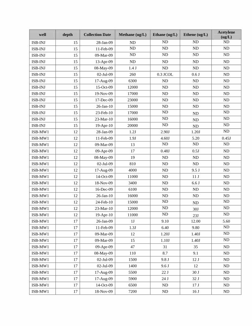
well depth Collection Date Methane (ug/L) Ethane (ug/L) Ethene (ug/L) Acetylene
(ug/L)
ISB-INJ 15 28-Jan-09 ND ND ND ND
ISB-INJ 15 11-Feb-09 ND ND ND ND
ISB-INJ 15 09-Mar-09 ND ND ND ND
ISB-INJ 15 13-Apr-09 ND ND ND ND
ISB-INJ 15 08-May-09 1.4 J ND ND ND
ISB-INJ 15 02-Jul-09 260 0.3 JCOL 0.6 J ND
ISB-INJ 15 17-Aug-09 6300 ND ND ND
ISB-INJ 15 15-Oct-09 12000 ND ND ND
ISB-INJ 15 19-Nov-09 17000 ND ND ND
ISB-INJ 15 17-Dec-09 23000 ND ND ND
ISB-INJ 15 26-Jan-10 15000 ND ND ND
ISB-INJ 15 23-Feb-10 17000 ND ND ND
ISB-INJ 15 23-Mar-10 16000 ND ND ND
ISB-INJ 15 19-Apr-10 20000 ND ND ND
ISB-MW1 12 28-Jan-09 1.2J 2.90J 1.20J ND
ISB-MW1 12 11-Feb-09 1.9J 4.60J 5.20 0.45J
ISB-MW1 12 09-Mar-09 13 ND ND ND
ISB-MW1 12 09-Apr-09 17 0.48J 0.5J ND
ISB-MW1 12 08-May-09 19 ND ND ND
ISB-MW1 12 02-Jul-09 810 ND ND ND
ISB-MW1 12 17-Aug-09 4000 ND 9.5 J ND
ISB-MW1 12 14-Oct-09 11000 ND 11 J ND
ISB-MW1 12 18-Nov-09 3400 ND 6.6 J ND
ISB-MW1 12 16-Dec-09 6100 ND ND ND
ISB-MW1 12 26-Jan-10 16000 ND ND ND
ISB-MW1 12 24-Feb-10 15000 ND ND ND
ISB-MW1 12 23-Mar-10 12000 ND 30J ND
ISB-MW1 12 19-Apr-10 11000 ND 23J ND
ISB-MW1 17 26-Jan-09 1J 9.10 12.00 5.60
ISB-MW1 17 11-Feb-09 1.3J 6.40 9.80 ND
ISB-MW1 17 09-Mar-09 12 1.20J 1.40J ND
ISB-MW1 17 09-Mar-09 15 1.10J 1.40J ND
ISB-MW1 17 09-Apr-09 47 31 35 ND
ISB-MW1 17 08-May-09 110 8.7 9.1 ND
ISB-MW1 17 02-Jul-09 1500 9.8 J 12 J ND
ISB-MW1 17 02-Jul-09 1400 9.6 J 12 ND
ISB-MW1 17 17-Aug-09 5500 22 J 30 J ND
ISB-MW1 17 17-Aug-09 5900 24 J 32 J ND
ISB-MW1 17 14-Oct-09 6500 ND 17 J ND
ISB-MW1 17 18-Nov-09 7200 ND 16 J ND

ISB-MW1 17 16-Dec-09 12000 ND ND ND
ISB-MW1 17 26-Jan-10 17000 ND 71 J ND
ISB-MW1 17 24-Feb-10 16000 ND 50J ND
ISB-MW1 17 23-Mar-10 14000 ND 22J ND
ISB-MW1 17 23-Mar-10 14000 ND 38J ND
ISB-MW1 17 19-Apr-10 16000 ND ND ND
ISB-MW1 22 28-Jan-09 0.46J 2.40J ND ND
ISB-MW1 22 11-Feb-09 1.3J 1.90J 2.40J ND
ISB-MW1 22 09-Mar-09 18 0.99J 1.30J ND
ISB-MW1 22 09-Apr-09 56 20 21 0.31
ISB-MW1 22 08-May-09 170 9 9.6 ND
ISB-MW1 22 02-Jul-09 1200 8.2 J 10 ND
ISB-MW1 22 17-Aug-09 4100 12 JCOL 15 J ND
ISB-MW1 22 14-Oct-09 2800 ND ND ND
ISB-MW1 22 18-Nov-09 5800 ND 150 ND
ISB-MW1 22 18-Nov-09 5700 ND 130 ND
ISB-MW1 22 16-Dec-09 13000 ND 66 J ND
ISB-MW1 22 26-Jan-10 19000 ND 130 J ND
ISB-MW1 22 24-Feb-10 18000 13J 160J ND
ISB-MW1 22 23-Mar-10 18000 64 130 ND
ISB-MW1 22 19-Apr-10 19000 89 150J ND
ISB-MW2 12 26-Jan-09 1.3J 4.20J 5.10 1.30J
ISB-MW2 12 11-Feb-09 1.4J 5.20 6.80 0.32J
ISB-MW2 12 09-Mar-09 12 2.10J 2.60J 0.00
ISB-MW2 12 09-Apr-09 16 6.6 8.7 0.89
ISB-MW2 12 08-May-09 63 1.4 J 1.2 JCOL ND
ISB-MW2 12 02-Jul-09 440 0.66 JCOL 0.99 J ND
ISB-MW2 12 17-Aug-09 4300 ND ND ND
ISB-MW2 12 15-Oct-09 4900 ND 160 ND
ISB-MW2 12 18-Nov-09 1700 6 J 84 6.5 J
ISB-MW2 12 17-Dec-09 7800 15 J 80 J ND
ISB-MW2 12 27-Jan-10 15000 ND 74 J ND
ISB-MW2 12 24-Feb-10 13000 ND 110J ND
ISB-MW2 12 22-Mar-10 11000 ND 77J ND
ISB-MW2 12 19-Apr-10 14000 ND 82J ND
ISB-MW2 17 26-Jan-09 0.73J 2.50J 3.70J 0.45J
ISB-MW2 17 11-Feb-09 0.92J 2.90J 4.80J ND
ISB-MW2 17 11-Feb-09 0.88J 2.80J 4.60J ND
ISB-MW2 17 09-Mar-09 7.9 1.10J 1.7J ND
ISB-MW2 17 09-Apr-09 35 15 20 0.45
ISB-MW2 17 08-May-09 260 4.5 J 6.2 ND

ISB-MW2 17 02-Jul-09 710 3.1 JCOL 4.8 J ND
ISB-MW2 17 17-Aug-09 4100 ND ND ND
ISB-MW2 17 15-Oct-09 6800 ND 530 ND
ISB-MW2 17 15-Oct-09 6400 ND 490 ND
ISB-MW2 17 18-Nov-09 5900 17 J 140 ND
ISB-MW2 17 17-Dec-09 11000 21 J 100 ND
ISB-MW2 17 27-Jan-10 17000 ND 130 J ND
ISB-MW2 17 27-Jan-10 17000 ND 120 J ND
ISB-MW2 17 24-Feb-10 15000 ND 130J ND
ISB-MW2 17 24-Feb-10 15000 ND 130J ND
ISB-MW2 17 22-Mar-10 14000 ND 100J ND
ISB-MW2 17 19-Apr-10 17000 ND 69J ND
ISB-MW2 17 19-Apr-10 16000 ND 97J ND
ISB-MW2 22 26-Jan-09 0.48J 0.48J ND ND
ISB-MW2 22 11-Feb-09 0.61J 0.66J 0.66J ND
ISB-MW2 22 09-Mar-09 12 0.95J 1.50J ND
ISB-MW2 22 09-Apr-09 19 8.7 12 ND
ISB-MW2 22 08-May-09 250 3.9 J 5.1 ND
ISB-MW2 22 02-Jul-09 620 2.7 J 3.9 J ND
ISB-MW2 22 17-Aug-09 3400 ND ND ND
ISB-MW2 22 15-Oct-09 8800 88 J 33 J ND
ISB-MW2 22 18-Nov-09 9100 17 J 300 ND
ISB-MW2 22 17-Dec-09 14000 14 J 180 J ND
ISB-MW2 22 27-Jan-10 16000 ND 330 ND
ISB-MW2 22 24-Feb-10 16000 28 340 ND
ISB-MW2 22 22-Mar-10 14000 92J 270 ND
ISB-MW2 22 19-Apr-10 17000 270 220 ND
ISB-MW3 12 27-Jan-09 0.32J ND ND ND
ISB-MW3 12 11-Feb-09 0.45J 0.25J ND ND
ISB-MW3 12 09-Mar-09 ND ND ND ND
ISB-MW3 12 09-Apr-09 0.36J 0.25J 0.64J ND
ISB-MW3 12 08-May-09 13 ND ND ND
ISB-MW3 12 02-Jul-09 1600 ND ND ND
ISB-MW3 12 17-Aug-09 5500 ND ND ND
ISB-MW3 12 14-Oct-09 12000 ND ND ND
ISB-MW3 12 19-Nov-09 13000 ND 19 J ND
ISB-MW3 12 17-Dec-09 18000 ND 290 ND
ISB-MW3 12 17-Dec-09 17000 ND 280 ND
ISB-MW3 12 27-Jan-10 24000 27 J 48 J ND
ISB-MW3 12 24-Feb-10 17000 ND 37J ND
ISB-MW3 12 22-Mar-10 12000 ND 41J ND
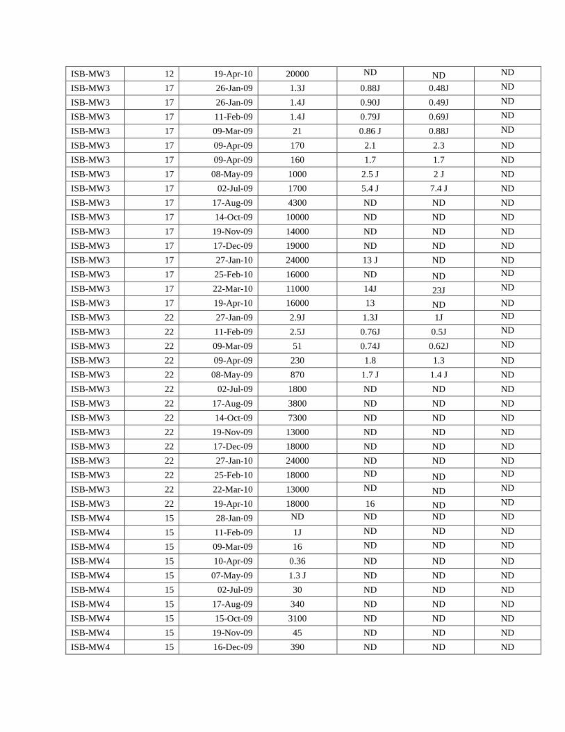
ISB-MW3 12 19-Apr-10 20000 ND ND ND
ISB-MW3 17 26-Jan-09 1.3J 0.88J 0.48J ND
ISB-MW3 17 26-Jan-09 1.4J 0.90J 0.49J ND
ISB-MW3 17 11-Feb-09 1.4J 0.79J 0.69J ND
ISB-MW3 17 09-Mar-09 21 0.86 J 0.88J ND
ISB-MW3 17 09-Apr-09 170 2.1 2.3 ND
ISB-MW3 17 09-Apr-09 160 1.7 1.7 ND
ISB-MW3 17 08-May-09 1000 2.5 J 2 J ND
ISB-MW3 17 02-Jul-09 1700 5.4 J 7.4 J ND
ISB-MW3 17 17-Aug-09 4300 ND ND ND
ISB-MW3 17 14-Oct-09 10000 ND ND ND
ISB-MW3 17 19-Nov-09 14000 ND ND ND
ISB-MW3 17 17-Dec-09 19000 ND ND ND
ISB-MW3 17 27-Jan-10 24000 13 J ND ND
ISB-MW3 17 25-Feb-10 16000 ND ND ND
ISB-MW3 17 22-Mar-10 11000 14J 23J ND
ISB-MW3 17 19-Apr-10 16000 13 ND ND
ISB-MW3 22 27-Jan-09 2.9J 1.3J 1J ND
ISB-MW3 22 11-Feb-09 2.5J 0.76J 0.5J ND
ISB-MW3 22 09-Mar-09 51 0.74J 0.62J ND
ISB-MW3 22 09-Apr-09 230 1.8 1.3 ND
ISB-MW3 22 08-May-09 870 1.7 J 1.4 J ND
ISB-MW3 22 02-Jul-09 1800 ND ND ND
ISB-MW3 22 17-Aug-09 3800 ND ND ND
ISB-MW3 22 14-Oct-09 7300 ND ND ND
ISB-MW3 22 19-Nov-09 13000 ND ND ND
ISB-MW3 22 17-Dec-09 18000 ND ND ND
ISB-MW3 22 27-Jan-10 24000 ND ND ND
ISB-MW3 22 25-Feb-10 18000 ND ND ND
ISB-MW3 22 22-Mar-10 13000 ND ND ND
ISB-MW3 22 19-Apr-10 18000 16 ND ND
ISB-MW4 15 28-Jan-09 ND ND ND ND
ISB-MW4 15 11-Feb-09 1J ND ND ND
ISB-MW4 15 09-Mar-09 16 ND ND ND
ISB-MW4 15 10-Apr-09 0.36 ND ND ND
ISB-MW4 15 07-May-09 1.3 J ND ND ND
ISB-MW4 15 02-Jul-09 30 ND ND ND
ISB-MW4 15 17-Aug-09 340 ND ND ND
ISB-MW4 15 15-Oct-09 3100 ND ND ND
ISB-MW4 15 19-Nov-09 45 ND ND ND
ISB-MW4 15 16-Dec-09 390 ND ND ND

ISB-MW4 15 26-Jan-10 3900 ND 15 J ND
ISB-MW4 15 23-Feb-10 3300 ND ND ND
ISB-MW4 15 23-Mar-10 3400 2.40J 26J ND
ISB-MW4 15 19-Apr-10 4100 ND ND ND
ISB-MW5 15 26-Jan-09 ND ND ND ND
ISB-MW5 15 11-Feb-09 4.3J ND ND ND
ISB-MW5 15 09-Mar-09 15 ND ND ND
ISB-MW5 15 13-Apr-09 0.87J ND ND ND
ISB-MW5 15 07-May-09 3 J ND ND ND
ISB-MW5 15 07-May-09 3 J ND ND ND
ISB-MW5 15 02-Jul-09 94 ND ND ND
ISB-MW5 15 17-Aug-09 720 ND ND ND
ISB-MW5 15 15-Oct-09 3700 ND ND ND
ISB-MW5 15 19-Nov-09 3400 ND ND ND
ISB-MW5 15 17-Dec-09 2400 ND ND ND
ISB-MW5 15 26-Jan-10 14000 ND ND ND
ISB-MW5 15 25-Feb-10 17000 ND ND ND
ISB-MW5 15 23-Mar-10 16000 ND ND ND
ISB-MW5 15 19-Apr-10 10000 ND ND ND
ISB-MW6 15 28-Jan-09 ND ND ND ND
ISB-MW6 15 11-Feb-09 14 ND ND ND
ISB-MW6 15 09-Mar-09 44 ND ND ND
ISB-MW6 15 10-Apr-09 0.74J ND ND ND
ISB-MW6 15 07-May-09 3 J ND ND ND
ISB-MW6 15 02-Jul-09 57 ND ND ND
ISB-MW6 15 17-Aug-09 540 ND ND ND
ISB-MW6 15 15-Oct-09 4400 ND ND ND
ISB-MW6 15 19-Nov-09 1800 ND ND ND
ISB-MW6 15 17-Dec-09 5500 ND ND ND
ISB-MW6 15 26-Jan-10 13000 ND ND ND
ISB-MW6 15 25-Feb-10 17000 ND ND ND
ISB-MW6 15 23-Mar-10 18000 ND ND ND
ISB-MW6 15 19-Apr-10 4800 ND ND ND

Table 5. ISB Analytical Results Redox Parameters and pH

Well Depth
(ft bgs) Collection Date
Sulfate
(mg/L)
Ferrous
Iron
(mg/L)
Nitrate as
N (mg/L)
Dissolved
Oxygen
(ppm)
ORP (Eh) pH
ISB-INJ 15 28-Jan-09 22 0.42 2 2.98 -60.2 6.07
ISB-INJ 15 11-Feb-09 15 0.41 0.0048 0.15 112 9.61
ISB-INJ 15 09-Mar-09 10 NS 0.05 0.11 153 6.68
ISB-INJ 15 13-Apr-09 0.42 NS 0.0078 JH 0.07 -237 8.4
ISB-INJ 15 08-May-09 0.16 J NS ND NS NS NS
ISB-INJ 15 02-Jul-09 0.88 2.3 HND NS NS NS
ISB-INJ 15 17-Aug-09 ND NS 0.43 J NS NS NS
ISB-INJ 15 15-Oct-09 ND 2.5 ND 0.3 -96 6.31 HF
ISB-INJ 15 19-Nov-09 0.61 J NS ND NS NS NS
ISB-INJ 15 17-Dec-09 ND 2.6 HND 0.74 53 6.64
ISB-INJ 15 26-Jan-10 1.1 J NS ND 0.48 31 6.05
ISB-INJ 15 23-Feb-10 0.64 J 2 ND 0.31 32 6.4
ISB-INJ 15 23-Mar-10 ND 4.5 ND 0.49 12 6.29
ISB-INJ 15 19-Apr-10 0.94 J 2.8 ND 0.26 36 6.10
ISB-MW1 12 28-Jan-09 19 NS 2.7 1.46 -106 6.2
ISB-MW1 12 11-Feb-09 17 5.4 0.0064 0.17 155 7.82
ISB-MW1 12 09-Mar-09 7.4 3.2 0.071 0.13 115 6.69
ISB-MW1 12 09-Apr-09 ND NS 0.0048 JH 0.08 -82 6.35
ISB-MW1 12 08-May-09 0.18 J NS ND 0.11 -148 6.25
ISB-MW1 12 02-Jul-09 0.66 B 2.8 HND 0.22 -100 6.71
ISB-MW1 12 17-Aug-09 ND 2.8 ND 0.41 -88 6.27
ISB-MW1 12 14-Oct-09 0.42 J 3.2 ND 0.4 -95 6.39 HF
ISB-MW1 12 18-Nov-09 4.6 2.8 ND 0.4 -5 5.65
ISB-MW1 12 16-Dec-09 1 J 2.6 ND 0.42 20 5.56
ISB-MW1 12 26-Jan-10 0.42 J NS ND 0.24 25 5.8
ISB-MW1 12 24-Feb-10 0.4 J 2.5 ND 0.39 41 5.9
ISB-MW1 12 23-Mar-10 ND 2.3 ND 0.37 23 6.06
ISB-MW1 12 19-Apr-10 1.3 2.7 ND 0.21 11 6.19
ISB-MW1 12 19-May-10 NS NS NS 0.20 15 5.95
ISB-MW1 17 28-Jan-09 19 0.42 1.80 1.87 -67.6 6.16
ISB-MW1 17 11-Feb-09 15 1.80 ND 0.17 168 7.89
ISB-MW1 17 09-Mar-09 3.1 11 0.0087 0.28 87 6.5
ISB-MW1 17 09-Mar-09 3.1 11 0.0084 0.28 87 6.5
ISB-MW1 17 09-Apr-09 0.32 * NS 0.012 JH 0.09 -78 6.39
ISB-MW1 17 08-May-09 0.18 J NS ND 0.1 -136 6.34
ISB-MW1 17 02-Jul-09 0.93 B 3.1 HND 0.22 -104 6.73
ISB-MW1 17 02-Jul-09 0.47 B NS HND 0.22 -104 6.73
ISB-MW1 17 17-Aug-09 ND 4.2 ND 0.39 -94 6.31
ISB-MW1 17 17-Aug-09 ND NS ND 0.39 -94 6.31
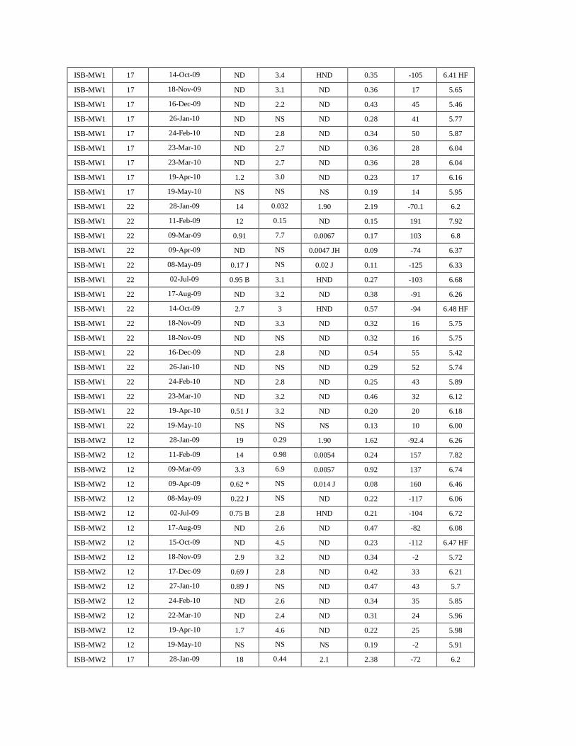
ISB-MW1 17 14-Oct-09 ND 3.4 HND 0.35 -105 6.41 HF
ISB-MW1 17 18-Nov-09 ND 3.1 ND 0.36 17 5.65
ISB-MW1 17 16-Dec-09 ND 2.2 ND 0.43 45 5.46
ISB-MW1 17 26-Jan-10 ND NS ND 0.28 41 5.77
ISB-MW1 17 24-Feb-10 ND 2.8 ND 0.34 50 5.87
ISB-MW1 17 23-Mar-10 ND 2.7 ND 0.36 28 6.04
ISB-MW1 17 23-Mar-10 ND 2.7 ND 0.36 28 6.04
ISB-MW1 17 19-Apr-10 1.2 3.0 ND 0.23 17 6.16
ISB-MW1 17 19-May-10 NS NS NS 0.19 14 5.95
ISB-MW1 22 28-Jan-09 14 0.032 1.90 2.19 -70.1 6.2
ISB-MW1 22 11-Feb-09 12 0.15 ND 0.15 191 7.92
ISB-MW1 22 09-Mar-09 0.91 7.7 0.0067 0.17 103 6.8
ISB-MW1 22 09-Apr-09 ND NS 0.0047 JH 0.09 -74 6.37
ISB-MW1 22 08-May-09 0.17 J NS 0.02 J 0.11 -125 6.33
ISB-MW1 22 02-Jul-09 0.95 B 3.1 HND 0.27 -103 6.68
ISB-MW1 22 17-Aug-09 ND 3.2 ND 0.38 -91 6.26
ISB-MW1 22 14-Oct-09 2.7 3 HND 0.57 -94 6.48 HF
ISB-MW1 22 18-Nov-09 ND 3.3 ND 0.32 16 5.75
ISB-MW1 22 18-Nov-09 ND NS ND 0.32 16 5.75
ISB-MW1 22 16-Dec-09 ND 2.8 ND 0.54 55 5.42
ISB-MW1 22 26-Jan-10 ND NS ND 0.29 52 5.74
ISB-MW1 22 24-Feb-10 ND 2.8 ND 0.25 43 5.89
ISB-MW1 22 23-Mar-10 ND 3.2 ND 0.46 32 6.12
ISB-MW1 22 19-Apr-10 0.51 J 3.2 ND 0.20 20 6.18
ISB-MW1 22 19-May-10 NS NS NS 0.13 10 6.00
ISB-MW2 12 28-Jan-09 19 0.29 1.90 1.62 -92.4 6.26
ISB-MW2 12 11-Feb-09 14 0.98 0.0054 0.24 157 7.82
ISB-MW2 12 09-Mar-09 3.3 6.9 0.0057 0.92 137 6.74
ISB-MW2 12 09-Apr-09 0.62 * NS 0.014 J 0.08 160 6.46
ISB-MW2 12 08-May-09 0.22 J NS ND 0.22 -117 6.06
ISB-MW2 12 02-Jul-09 0.75 B 2.8 HND 0.21 -104 6.72
ISB-MW2 12 17-Aug-09 ND 2.6 ND 0.47 -82 6.08
ISB-MW2 12 15-Oct-09 ND 4.5 ND 0.23 -112 6.47 HF
ISB-MW2 12 18-Nov-09 2.9 3.2 ND 0.34 -2 5.72
ISB-MW2 12 17-Dec-09 0.69 J 2.8 ND 0.42 33 6.21
ISB-MW2 12 27-Jan-10 0.89 J NS ND 0.47 43 5.7
ISB-MW2 12 24-Feb-10 ND 2.6 ND 0.34 35 5.85
ISB-MW2 12 22-Mar-10 ND 2.4 ND 0.31 24 5.96
ISB-MW2 12 19-Apr-10 1.7 4.6 ND 0.22 25 5.98
ISB-MW2 12 19-May-10 NS NS NS 0.19 -2 5.91
ISB-MW2 17 28-Jan-09 18 0.44 2.1 2.38 -72 6.2

ISB-MW2 17 11-Feb-09 14 0.59 0.0047 0.18 174 7.84
ISB-MW2 17 11-Feb-09 14 0.62 0.0047 0.18 174 7.84
ISB-MW2 17 09-Mar-09 2.2 7.4 ND 1.58 118 6.78
ISB-MW2 17 09-Apr-09 0.41 * NS 0.018 JH 0.05 155 6.45
ISB-MW2 17 08-May-09 0.17 J NS 0.01 J 0.14 -123 6.27
ISB-MW2 17 02-Jul-09 0.53 B 2.1 HND 0.2 -106 6.79
ISB-MW2 17 17-Aug-09 ND 2.8 0.89 J 0.41 -94 6.32
ISB-MW2 17 15-Oct-09 ND 4.4 ND 0.31 -113 6.46 HF
ISB-MW2 17 15-Oct-09 ND NS HND 0.31 -113 6.46 HF
ISB-MW2 17 18-Nov-09 ND 3.1 ND 0.33 17 5.71
ISB-MW2 17 17-Dec-09 ND 2.8 ND 0.46 41 6.19
ISB-MW2 17 27-Jan-10 ND NS ND 0.45 45 5.73
ISB-MW2 17 27-Jan-10 ND NS ND 0.45 45 5.73
ISB-MW2 17 24-Feb-10 ND 3.2 ND 0.37 43 5.87
ISB-MW2 17 24-Feb-10 ND 3.2 ND 0.37 43 5.87
ISB-MW2 17 22-Mar-10 ND 2.7 ND 0.35 33 5.98
ISB-MW2 17 19-Apr-10 0.46 J 5.0 ND 0.20 29 6.07
ISB-MW2 17 19-Apr-10 0.43 J 5.0 ND 0.20 29 6.07
ISB-MW2 17 19-May-10 NS NS NS 0.20 -8 6.04
ISB-MW2 22 28-Jan-09 16 0.067 2.1 2.59 -79.1 6.17
ISB-MW2 22 11-Feb-09 12 0.71 ND 0.18 166 7.9
ISB-MW2 22 09-Mar-09 0.64 6.9 ND 0.91 102 6.44
ISB-MW2 22 09-Apr-09 0.36 * NS 0.0065 JH 0.07 184 6.42
ISB-MW2 22 08-May-09 0.14 J NS 0.01 J 0.1 -114 6.24
ISB-MW2 22 02-Jul-09 0.33 2.8 HND 0.18 -101 6.75
ISB-MW2 22 17-Aug-09 ND 2.2 ND 0.37 -85 6.29
ISB-MW2 22 15-Oct-09 0.57 J 3.4 ND 0.29 -105 6.46 HF
ISB-MW2 22 18-Nov-09 ND 1.1 ND 0.33 30 5.68
ISB-MW2 22 17-Dec-09 ND 2.4 ND 0.5 50 6.18
ISB-MW2 22 27-Jan-10 ND NS ND 0.44 48 5.68
ISB-MW2 22 24-Feb-10 ND 3.9 ND 0.31 46 5.82
ISB-MW2 22 22-Mar-10 ND 2.5 ND 0.29 32 5.98
ISB-MW2 22 19-Apr-10 0.67 J 3.0 ND 0.19 41 6.09
ISB-MW2 22 19-May-10 NS NS NS 0.20 5 5.90
ISB-MW3 12 28-Jan-09 22 ND 2.1 3.06 -109 6.1
ISB-MW3 12 11-Feb-09 16 0.1 ND 0.28 256 7.5
ISB-MW3 12 09-Mar-09 6.1 7.3 0.045 0.1 119 6.75
ISB-MW3 12 09-Apr-09 0.27 J* NS 0.015 JH 0.09 -109 6.17
ISB-MW3 12 08-May-09 0.15 J NS ND 0.08 -128 6.23
ISB-MW3 12 02-Jul-09 0.42 2.6 HND 0.2 -94 6.71
ISB-MW3 12 17-Aug-09 ND 3.2 ND 0.33 -92 6.22

ISB-MW3 12 14-Oct-09 ND 2.2 HND 0.3 -100 6.28 HF
ISB-MW3 12 19-Nov-09 2.4 2.2 ND 0.23 12 6.15
ISB-MW3 12 17-Dec-09 ND 2.5 ND 0.42 41 6.25
ISB-MW3 12 17-Dec-09 ND NS ND 0.42 41 6.25
ISB-MW3 12 27-Jan-10 ND NS ND 0.36 14 5.82
ISB-MW3 12 24-Feb-10 ND 2.7 ND 0.3 14 6
ISB-MW3 12 22-Mar-10 ND 2.3 ND 0.27 15 6.15
ISB-MW3 12 19-Apr-10 ND 4.2 ND 0.23 39 6.13
ISB-MW3 12 19-May-10 NS NS NS 0.21 -3 5.99
ISB-MW3 17 28-Jan-09 14 ND 1.7 2.48 -64 6.24
ISB-MW3 17 28-Jan-09 14 ND 1.7 2.48 -64 6.24
ISB-MW3 17 11-Feb-09 9.4 0.051 0.007 0.24 201 7.61
ISB-MW3 17 09-Mar-09 3.2 8.5 0.01 0.42 112 6.73
ISB-MW3 17 09-Apr-09 0.67 * NS 0.014 JH 0.1 -127 6.28
ISB-MW3 17 09-Apr-09 0.65 * NS 0.015 JH 0.1 -127 6.28
ISB-MW3 17 08-May-09 0.17 J NS ND 0.09 -136 6.41
ISB-MW3 17 02-Jul-09 1.8 2.8 HND 0.2 -97 6.81
ISB-MW3 17 17-Aug-09 ND 4 ND 0.34 -95 6.26
ISB-MW3 17 14-Oct-09 0.4 J 2.6 HND 0.24 -116 6.52 HF
ISB-MW3 17 19-Nov-09 ND 2.3 ND 0.27 30 6.24
ISB-MW3 17 17-Dec-09 ND 2 ND 0.43 41 6.39
ISB-MW3 17 27-Jan-10 ND NS ND 0.38 28 5.93
ISB-MW3 17 25-Feb-10 ND 3.4 ND 0.44 12 6.13
ISB-MW3 17 22-Mar-10 ND 2.3 ND 0.31 0 6.15
ISB-MW3 17 19-Apr-10 ND 4.0 ND 0.23 29 6.15
ISB-MW3 17 19-May-10 NS NS NS 0.19 -9 6.07
ISB-MW3 22 28-Jan-09 8.7 1 1.2 2.5 -137 6.44
ISB-MW3 22 11-Feb-09 6 0.0.51 0.18 0.24 164 7.65
ISB-MW3 22 09-Mar-09 3.7 8.3 0.19 0.12 105 6.82
ISB-MW3 22 09-Apr-09 2.4 * NS 0.018 J 0.12 -134 6.22
ISB-MW3 22 08-May-09 2 NS 0.01 J 0.09 -157 6.35
ISB-MW3 22 02-Jul-09 1.8 3.8 HND 0.2 -100 6.86
ISB-MW3 22 17-Aug-09 ND 3.8 0.46 J 0.35 -103 6.32
ISB-MW3 22 14-Oct-09 0.67 J 2 HND 0.3 -123 6.51 HF
ISB-MW3 22 19-Nov-09 ND 3 ND 0.23 22 6.31
ISB-MW3 22 17-Dec-09 ND 2.2 ND 0.47 38 6.39
ISB-MW3 22 27-Jan-10 ND NS ND 0.36 18 5.92
ISB-MW3 22 25-Feb-10 ND 3.5 ND 0.37 8 6.14
ISB-MW3 22 22-Mar-10 ND 3.4 ND 0.28 -3 6.22
ISB-MW3 22 19-Apr-10 0.47 J 3.4 ND 0.21 24 6.21
ISB-MW3 22 19-May-10 NS NS NS 0.20 -17 6.04
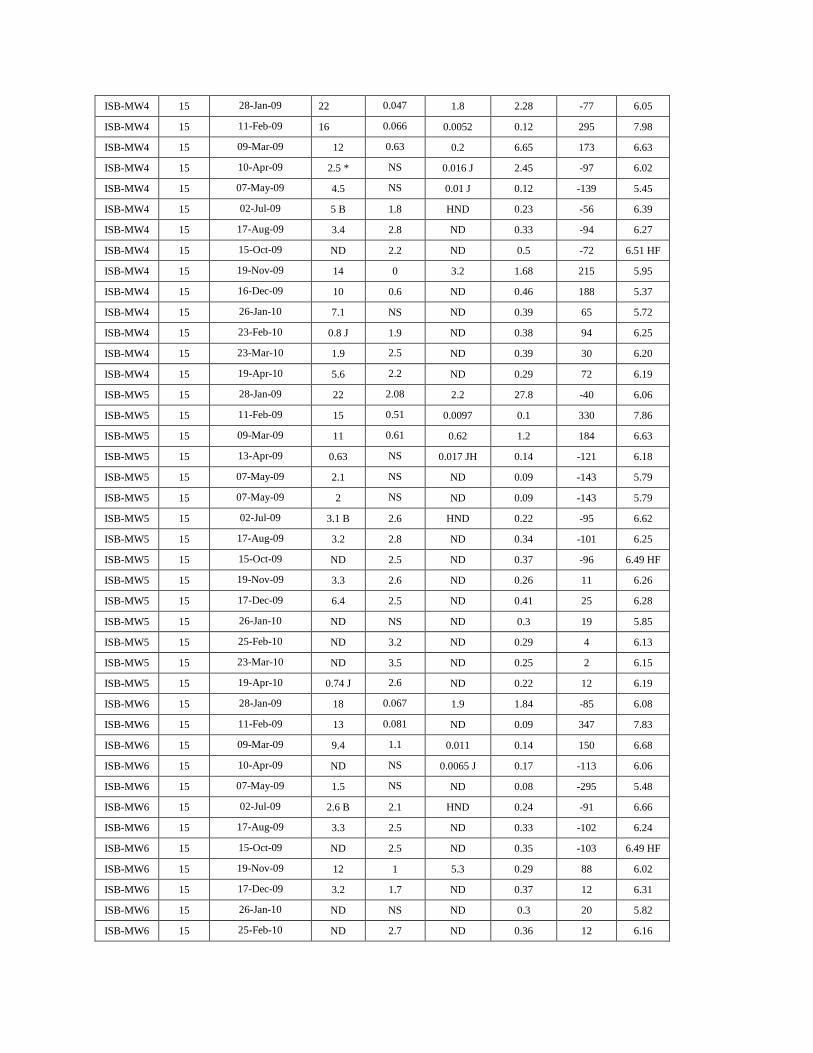
ISB-MW4 15 28-Jan-09 22 0.047 1.8 2.28 -77 6.05
ISB-MW4 15 11-Feb-09 16 0.066 0.0052 0.12 295 7.98
ISB-MW4 15 09-Mar-09 12 0.63 0.2 6.65 173 6.63
ISB-MW4 15 10-Apr-09 2.5 * NS 0.016 J 2.45 -97 6.02
ISB-MW4 15 07-May-09 4.5 NS 0.01 J 0.12 -139 5.45
ISB-MW4 15 02-Jul-09 5 B 1.8 HND 0.23 -56 6.39
ISB-MW4 15 17-Aug-09 3.4 2.8 ND 0.33 -94 6.27
ISB-MW4 15 15-Oct-09 ND 2.2 ND 0.5 -72 6.51 HF
ISB-MW4 15 19-Nov-09 14 0 3.2 1.68 215 5.95
ISB-MW4 15 16-Dec-09 10 0.6 ND 0.46 188 5.37
ISB-MW4 15 26-Jan-10 7.1 NS ND 0.39 65 5.72
ISB-MW4 15 23-Feb-10 0.8 J 1.9 ND 0.38 94 6.25
ISB-MW4 15 23-Mar-10 1.9 2.5 ND 0.39 30 6.20
ISB-MW4 15 19-Apr-10 5.6 2.2 ND 0.29 72 6.19
ISB-MW5 15 28-Jan-09 22 2.08 2.2 27.8 -40 6.06
ISB-MW5 15 11-Feb-09 15 0.51 0.0097 0.1 330 7.86
ISB-MW5 15 09-Mar-09 11 0.61 0.62 1.2 184 6.63
ISB-MW5 15 13-Apr-09 0.63 NS 0.017 JH 0.14 -121 6.18
ISB-MW5 15 07-May-09 2.1 NS ND 0.09 -143 5.79
ISB-MW5 15 07-May-09 2 NS ND 0.09 -143 5.79
ISB-MW5 15 02-Jul-09 3.1 B 2.6 HND 0.22 -95 6.62
ISB-MW5 15 17-Aug-09 3.2 2.8 ND 0.34 -101 6.25
ISB-MW5 15 15-Oct-09 ND 2.5 ND 0.37 -96 6.49 HF
ISB-MW5 15 19-Nov-09 3.3 2.6 ND 0.26 11 6.26
ISB-MW5 15 17-Dec-09 6.4 2.5 ND 0.41 25 6.28
ISB-MW5 15 26-Jan-10 ND NS ND 0.3 19 5.85
ISB-MW5 15 25-Feb-10 ND 3.2 ND 0.29 4 6.13
ISB-MW5 15 23-Mar-10 ND 3.5 ND 0.25 2 6.15
ISB-MW5 15 19-Apr-10 0.74 J 2.6 ND 0.22 12 6.19
ISB-MW6 15 28-Jan-09 18 0.067 1.9 1.84 -85 6.08
ISB-MW6 15 11-Feb-09 13 0.081 ND 0.09 347 7.83
ISB-MW6 15 09-Mar-09 9.4 1.1 0.011 0.14 150 6.68
ISB-MW6 15 10-Apr-09 ND NS 0.0065 J 0.17 -113 6.06
ISB-MW6 15 07-May-09 1.5 NS ND 0.08 -295 5.48
ISB-MW6 15 02-Jul-09 2.6 B 2.1 HND 0.24 -91 6.66
ISB-MW6 15 17-Aug-09 3.3 2.5 ND 0.33 -102 6.24
ISB-MW6 15 15-Oct-09 ND 2.5 ND 0.35 -103 6.49 HF
ISB-MW6 15 19-Nov-09 12 1 5.3 0.29 88 6.02
ISB-MW6 15 17-Dec-09 3.2 1.7 ND 0.37 12 6.31
ISB-MW6 15 26-Jan-10 ND NS ND 0.3 20 5.82
ISB-MW6 15 25-Feb-10 ND 2.7 ND 0.36 12 6.16

ISB-MW6 15 23-Mar-10 ND 2.5 ND 0.3 12 6.17
ISB-MW6 15 19-Apr-10 2.7 2.8 ND 0.19 8 6.18
ND: Non Detect NS: Not Sampled

Table 6. ISB Analytical Results Chlorinated Ethenes
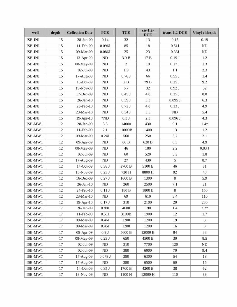
well depth Collection Date PCE TCE cis-1,2-
DCE trans-1,2-DCE Vinyl chloride
ISB-INJ 15 28-Jan-09 0.14 32 13 0.15 0.19
ISB-INJ 15 11-Feb-09 0.096J 85 18 0.51J ND
ISB-INJ 15 09-Mar-09 0.086J 25 23 0.36J ND
ISB-INJ 15 13-Apr-09 ND 3.9 B 17 B 0.19 J 1.2
ISB-INJ 15 08-May-09 ND 2 19 0.17 J 1.3
ISB-INJ 15 02-Jul-09 ND 1.9 43 1.1 2.3
ISB-INJ 15 17-Aug-09 ND 0.78 J 66 0.55 J 1.4
ISB-INJ 15 15-Oct-09 ND 2 B 79 B 0.25 J 9.2
ISB-INJ 15 19-Nov-09 ND 6.7 32 0.92 J 52
ISB-INJ 15 17-Dec-09 ND 0.45 J 4.8 0.25 J 8.8
ISB-INJ 15 26-Jan-10 ND 0.39 J 3.3 0.095 J 6.3
ISB-INJ 15 23-Feb-10 ND 0.72 J 4.8 0.13 J 4.9
ISB-INJ 15 23-Mar-10 ND 0.34 J 3.5 ND 5.4
ISB-INJ 15 19-Apr-10 *ND 0.3 J 2.3 0.096 J 4.3
ISB-MW1 12 28-Jan-09 3.5 14000 430 9.1 1.4*
ISB-MW1 12 11-Feb-09 2.1 10000B 1400 13 1.2
ISB-MW1 12 09-Mar-09 0.24J 560 250 3.7 2.1
ISB-MW1 12 09-Apr-09 ND 66 B 620 B 6.3 4.9
ISB-MW1 12 08-May-09 ND 46 180 2.2 0.83 J
ISB-MW1 12 02-Jul-09 ND 60 520 5.3 1.8
ISB-MW1 12 17-Aug-09 ND 27 430 5 8.7
ISB-MW1 12 14-Oct-09 0.38 J 2700 B 5100 B 46 81
ISB-MW1 12 18-Nov-09 0.23 J 720 H 8800 H 92 40
ISB-MW1 12 16-Dec-09 0.27 J 1600 B 1300 8 5.9
ISB-MW1 12 26-Jan-10 ND 260 2500 7.1 21
ISB-MW1 12 24-Feb-10 0.11 J 180 B 1800 B 8 150
ISB-MW1 12 23-Mar-10 ND 69 610 5.4 110
ISB-MW1 12 19-Apr-10 0.17 J 310 2100 20 230
ISB-MW1 17 26-Jan-09 0.88J 4600 190 1.4 2.2*
ISB-MW1 17 11-Feb-09 0.51J 3100B 1900 12 1.7
ISB-MW1 17 09-Mar-09 0.46J 1200 1200 19 3
ISB-MW1 17 09-Mar-09 0.45J 1200 1200 16 3
ISB-MW1 17 09-Apr-09 0.9 J 5600 B 12000 B 84 38
ISB-MW1 17 08-May-09 0.23 J 650 4500 B 30 8.5
ISB-MW1 17 02-Jul-09 ND 310 7700 120 ND
ISB-MW1 17 02-Jul-09 ND 380 6900 70 9.4
ISB-MW1 17 17-Aug-09 0.078 J 380 6300 54 18
ISB-MW1 17 17-Aug-09 ND 380 6500 60 15
ISB-MW1 17 14-Oct-09 0.35 J 1700 B 4200 B 38 62
ISB-MW1 17 18-Nov-09 ND 1100 H 12000 H 110 89

ISB-MW1 17 16-Dec-09 0.88 J 5200 B 6300 19 44
ISB-MW1 17 26-Jan-10 0.32 J 3400 8400 46 460
ISB-MW1 17 24-Feb-10 0.092 J 520 B 2500 B 7.7 82
ISB-MW1 17 23-Mar-10 ND 960 3300 33 55
ISB-MW1 17 23-Mar-10 ND 830 3300 35 57
ISB-MW1 17 19-Apr-10 0.73 J 5300 8500 54 110
ISB-MW1 22 28-Jan-09 0.87J 2900B 73 0.61J 0.43J
ISB-MW1 22 11-Feb-09 0.54J 3100B 400 3.7 0.52J
ISB-MW1 22 09-Mar-09 0.54J 2000 1600 28 11
ISB-MW1 22 09-Apr-09 0.9 J 4400 B 15000 B 130 49
ISB-MW1 22 08-May-09 0.28 J 930 7800 69 18
ISB-MW1 22 02-Jul-09 0.23 J 830 H 13000 H 130 H 16
ISB-MW1 22 17-Aug-09 0.42 J 2100 12000 91 17
ISB-MW1 22 14-Oct-09 0.23 J 50 B 900 B 6.7 63
ISB-MW1 22 18-Nov-09 ND 57 4000 H 45 550 H
ISB-MW1 22 18-Nov-09 ND 69 H 4700 H 46 570 H
ISB-MW1 22 16-Dec-09 0.17 J 360 B 8600 22 140
ISB-MW1 22 26-Jan-10 0.13 J 450 9600 58 660
ISB-MW1 22 24-Feb-10 0.13 J 140 3300 B 19 290
ISB-MW1 22 23-Mar-10 ND 53 3200 47 410
ISB-MW1 22 19-Apr-10 0.12 J 100 3600 30 780
ISB-MW2 12 26-Jan-09 5.7 19000B 4100 65 3*
ISB-MW2 12 11-Feb-09 4.9 25000 7500 89 2
ISB-MW2 12 09-Mar-09 3.5 11000 4200 73 3.8
ISB-MW2 12 09-Apr-09 12 38000 B 17000 B 330 43
ISB-MW2 12 08-May-09 3.5 8100 11000 B 140 10
ISB-MW2 12 02-Jul-09 0.93 J 2300 9500 130 4.5
ISB-MW2 12 17-Aug-09 0.83 J 2800 8200 85 13
ISB-MW2 12 15-Oct-09 2.8 13000 B 11000 B 140 780
ISB-MW2 12 18-Nov-09 11 26000 H 19000 H 190 H 440 H
ISB-MW2 12 17-Dec-09 22 42000 B 20000 85 150
ISB-MW2 12 27-Jan-10 18 32000 24000 330 360
ISB-MW2 12 24-Feb-10 7.3 12000 14000 52 190
ISB-MW2 12 22-Mar-10 3.5 9400 23000 120 170
ISB-MW2 12 19-Apr-10 17 36000 57000 B 220 280
ISB-MW2 17 26-Jan-09 0.94J 6300B 530 4.5 0.7J*
ISB-MW2 17 11-Feb-09 0.9J 7600B 1400 12 0.78J
ISB-MW2 17 11-Feb-09 0.84J 7200B 1300 13 0.69J
ISB-MW2 17 09-Mar-09 0.87J 4900 1900 30 3.5
ISB-MW2 17 09-Apr-09 1.9 16000 B 16000 B 120 54
ISB-MW2 17 08-May-09 0.68 J 5000 10000 B 89 17
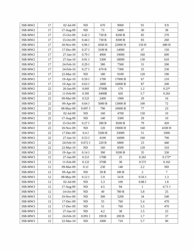
ISB-MW2 17 02-Jul-09 ND 670 9000 91 9.9
ISB-MW2 17 17-Aug-09 ND 73 5400 30 38
ISB-MW2 17 15-Oct-09 0.42 J 730 B 8200 B 85 270
ISB-MW2 17 15-Oct-09 0.44 J 730 B 8300 B 83 260
ISB-MW2 17 18-Nov-09 0.96 J 4500 H 22000 H 150 H 680 H
ISB-MW2 17 17-Dec-09 0.37 J 3100 B 14000 47 150
ISB-MW2 17 27-Jan-10 0.79 J 4900 19000 160 600
ISB-MW2 17 27-Jan-10 0.91 J 5300 18000 130 610
ISB-MW2 17 24-Feb-10 0.29 J 580 7500 31 200
ISB-MW2 17 24-Feb-10 0.27 J 670 B 7300 25 230
ISB-MW2 17 22-Mar-10 ND 180 9100 120 190
ISB-MW2 17 19-Apr-10 0.59 J 1700 17000 B 67 210
ISB-MW2 17 19-Apr-10 0.63 J 1800 16000 B 87 200
ISB-MW2 22 26-Jan-09 0.69J 3700B 170 1.2 0.2J*
ISB-MW2 22 11-Feb-09 0.39J 3400B 420 5.7 0.26J
ISB-MW2 22 09-Mar-09 0.52J 2400 1900 29 16
ISB-MW2 22 09-Apr-09 0.64 J 5000 B 13000 B 100 72
ISB-MW2 22 08-May-09 0.097 J 790 10000 B 77 23
ISB-MW2 22 02-Jul-09 ND 160 4700 150 10
ISB-MW2 22 17-Aug-09 ND 140 3300 29 10
ISB-MW2 22 15-Oct-09 0.27 J 280 B 8500 B 79 420
ISB-MW2 22 18-Nov-09 ND 120 19000 H 160 4100 H
ISB-MW2 22 17-Dec-09 0.4 J 5500 B 33000 51 1000
ISB-MW2 22 27-Jan-10 0.53 J 4100 16000 160 790
ISB-MW2 22 24-Feb-10 0.072 J 220 B 6800 23 440
ISB-MW2 22 22-Mar-10 ND 160 8500 120 310
ISB-MW2 22 19-Apr-10 0.14 J 390 9200 B 35 330
ISB-MW3 12 27-Jan-09 0.21J 170B 25 0.26J 0.17J*
ISB-MW3 12 11-Feb-09 0.12J 370B 38 0.57J 0.16J
ISB-MW3 12 09-Mar-09 0.1J 230 140 2.2 ND
ISB-MW3 12 09-Apr-09 ND 39 B 180 B 2 7
ISB-MW3 12 08-May-09 0.12 J 5.9 54 B 0.56 J 1.3
ISB-MW3 12 02-Jul-09 ND 5.3 100 0.88 J 1.8
ISB-MW3 12 17-Aug-09 ND 4.5 94 1 0.71 J
ISB-MW3 12 14-Oct-09 ND 40 780 B 5.8 25
ISB-MW3 12 19-Nov-09 ND 300 5200 34 540
ISB-MW3 12 17-Dec-09 ND 55 760 5.4 470
ISB-MW3 12 17-Dec-09 ND 51 760 5.5 470
ISB-MW3 12 27-Jan-10 ND 4.2 38 1.5 23
ISB-MW3 12 24-Feb-10 0.091 J 190 B 200 B 1.7 37
ISB-MW3 12 22-Mar-10 ND 1000 710 5.7 90
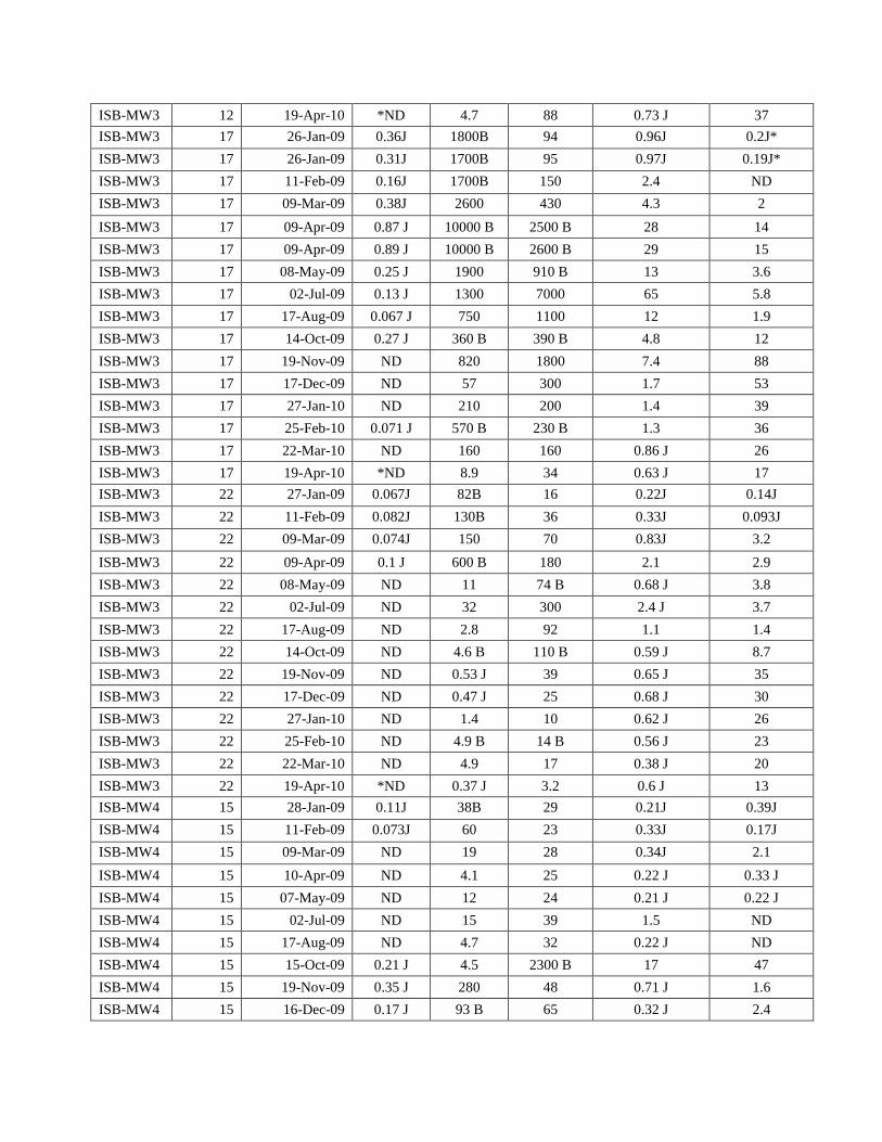
ISB-MW3 12 19-Apr-10 *ND 4.7 88 0.73 J 37
ISB-MW3 17 26-Jan-09 0.36J 1800B 94 0.96J 0.2J*
ISB-MW3 17 26-Jan-09 0.31J 1700B 95 0.97J 0.19J*
ISB-MW3 17 11-Feb-09 0.16J 1700B 150 2.4 ND
ISB-MW3 17 09-Mar-09 0.38J 2600 430 4.3 2
ISB-MW3 17 09-Apr-09 0.87 J 10000 B 2500 B 28 14
ISB-MW3 17 09-Apr-09 0.89 J 10000 B 2600 B 29 15
ISB-MW3 17 08-May-09 0.25 J 1900 910 B 13 3.6
ISB-MW3 17 02-Jul-09 0.13 J 1300 7000 65 5.8
ISB-MW3 17 17-Aug-09 0.067 J 750 1100 12 1.9
ISB-MW3 17 14-Oct-09 0.27 J 360 B 390 B 4.8 12
ISB-MW3 17 19-Nov-09 ND 820 1800 7.4 88
ISB-MW3 17 17-Dec-09 ND 57 300 1.7 53
ISB-MW3 17 27-Jan-10 ND 210 200 1.4 39
ISB-MW3 17 25-Feb-10 0.071 J 570 B 230 B 1.3 36
ISB-MW3 17 22-Mar-10 ND 160 160 0.86 J 26
ISB-MW3 17 19-Apr-10 *ND 8.9 34 0.63 J 17
ISB-MW3 22 27-Jan-09 0.067J 82B 16 0.22J 0.14J
ISB-MW3 22 11-Feb-09 0.082J 130B 36 0.33J 0.093J
ISB-MW3 22 09-Mar-09 0.074J 150 70 0.83J 3.2
ISB-MW3 22 09-Apr-09 0.1 J 600 B 180 2.1 2.9
ISB-MW3 22 08-May-09 ND 11 74 B 0.68 J 3.8
ISB-MW3 22 02-Jul-09 ND 32 300 2.4 J 3.7
ISB-MW3 22 17-Aug-09 ND 2.8 92 1.1 1.4
ISB-MW3 22 14-Oct-09 ND 4.6 B 110 B 0.59 J 8.7
ISB-MW3 22 19-Nov-09 ND 0.53 J 39 0.65 J 35
ISB-MW3 22 17-Dec-09 ND 0.47 J 25 0.68 J 30
ISB-MW3 22 27-Jan-10 ND 1.4 10 0.62 J 26
ISB-MW3 22 25-Feb-10 ND 4.9 B 14 B 0.56 J 23
ISB-MW3 22 22-Mar-10 ND 4.9 17 0.38 J 20
ISB-MW3 22 19-Apr-10 *ND 0.37 J 3.2 0.6 J 13
ISB-MW4 15 28-Jan-09 0.11J 38B 29 0.21J 0.39J
ISB-MW4 15 11-Feb-09 0.073J 60 23 0.33J 0.17J
ISB-MW4 15 09-Mar-09 ND 19 28 0.34J 2.1
ISB-MW4 15 10-Apr-09 ND 4.1 25 0.22 J 0.33 J
ISB-MW4 15 07-May-09 ND 12 24 0.21 J 0.22 J
ISB-MW4 15 02-Jul-09 ND 15 39 1.5 ND
ISB-MW4 15 17-Aug-09 ND 4.7 32 0.22 J ND
ISB-MW4 15 15-Oct-09 0.21 J 4.5 2300 B 17 47
ISB-MW4 15 19-Nov-09 0.35 J 280 48 0.71 J 1.6
ISB-MW4 15 16-Dec-09 0.17 J 93 B 65 0.32 J 2.4

ISB-MW4 15 26-Jan-10 ND 20 340 1.6 52
ISB-MW4 15 23-Feb-10 ND 4.5 99 0.89 J 31
ISB-MW4 15 23-Mar-10 ND 3.1 89 0.94 J 68
ISB-MW4 15 19-Apr-10 *ND 7.5 180 1.1 43
ISB-MW5 15 26-Jan-09 0.12J 35B 23 0.19J 0.22J
ISB-MW5 15 11-Feb-09 ND 57 23 0.3J 0.39J
ISB-MW5 15 09-Mar-09 ND 22 31 0.28J 2.1
ISB-MW5 15 13-Apr-09 ND 3.4 B 25 B 0.24 J 0.46 J
ISB-MW5 15 07-May-09 ND 4.5 21 0.21 J 0.32 J
ISB-MW5 15 07-May-09 ND 4.2 22 0.26 J 0.26 J
ISB-MW5 15 02-Jul-09 ND 2.3 24 2.3 ND
ISB-MW5 15 17-Aug-09 ND 2.3 22 0.2 J ND
ISB-MW5 15 15-Oct-09 ND 1.1 B 30 B ND 0.79 J
ISB-MW5 15 19-Nov-09 ND 8.3 78 0.35 J 3.3
ISB-MW5 15 17-Dec-09 ND 2.5 27 0.16 J 2.9
ISB-MW5 15 26-Jan-10 ND 0.35 J 14 0.21 J 16
ISB-MW5 15 25-Feb-10 ND 0.44 J B 11 B 0.24 J 11
ISB-MW5 15 23-Mar-10 ND 0.38 J 9.4 ND 11
ISB-MW5 15 19-Apr-10 *ND 1.2 8.1 0.14 J 8
ISB-MW6 15 28-Jan-09 0.12J 33B 23 0.19J 0.27J
ISB-MW6 15 11-Feb-09 0.11J 48 21 0.3J 1.1
ISB-MW6 15 09-Mar-09 ND 23 26 0.44J 3.5
ISB-MW6 15 10-Apr-09 ND 1.8 B 21 B 0.21 J 0.49 J
ISB-MW6 15 07-May-09 ND 2.9 18 0.2 J 0.34 J
ISB-MW6 15 02-Jul-09 ND 2.1 19 1.6 ND
ISB-MW6 15 17-Aug-09 ND 1.9 23 ND ND
ISB-MW6 15 15-Oct-09 ND 1.1 B 34 B 0.073 J 0.78 J
ISB-MW6 15 19-Nov-09 ND 85 54 0.28 J 1 J
ISB-MW6 15 17-Dec-09 ND 1.5 26 0.14 J 1.7
ISB-MW6 15 26-Jan-10 ND 0.37 J 14 0.1 J 6.5
ISB-MW6 15 25-Feb-10 ND 0.29 J B 12 B 0.14 J 7.9
ISB-MW6 15 23-Mar-10 ND 0.13 J 8.4 ND 8.7
ISB-MW6 15 19-Apr-10 *ND 3.1 12 0.07 J 3.7

Table 7. ZVI Analytical Results Dissolved Gasses

well depth Collection
Date Methane Ethane Ethene Chloride Acetylene
ft ug/L ug/L ug/L mg/L ug/L
ZVI-INJ 13 13-Apr-09 3.8 4.3 7.4 4.3 0.33
ZVI-INJ 13 22-Apr-09 96 79 60 2.91 ND
ZVI-INJ 13 28-Apr-09 78 62 46 3.05 0.44J
ZVI-INJ 13 07-May-09 71 31 26 3.2 2.3J
ZVI-INJ 13 29-May-09 93 21 20 2.8 0.67J
ZVI-INJ 13 18-Jun-09 160 62 90 4B 0.94J
ZVI-INJ 13 26-Jun-09 470 44 55 3.1 ND
ZVI-INJ 13 01-Jul-09 1700 68 130 4.5 ND
ZVI-INJ 13 10-Jul-09 2900 63COL 160 6.9 3.9JCOL
ZVI-INJ 13 15-Jul-09 1400 59 180 8.4 5.9J
ZVI-INJ 13 23-Jul-09 1600 58 140 9.7 7.4J
ZVI-INJ 13 28-Jul-09 610 38 95 11 7
ZVI-INJ 13 06-Aug-09 1000 43 86 16 5.4J
ZVI-INJ 13 14-Aug-09 1100 44 73 13 11
ZVI-INJ 13 19-Aug-09 1500 48J 64 9.7 8.4J
ZVI-INJ 13 27-Aug-09 3300 66 70 6.3 6.2J
ZVI-INJ 13 10-Sep-09 3400 57 56 6.7 ND
ZVI-INJ 13 16-Oct-09 5300 76 40J 4.5 ND
ZVI-INJ 13 29-Oct-09 5700 97 110 32 ND
ZVI-INJ 13 12-Nov-09 5400 160 200 56 ND
ZVI-INJ 13 26-Mar-10 5300H 120H 210H 12 ND ZVI-
MW1 13 13-Apr-09 ND ND ND 2.4 ND ZVI-
MW1 13 21-Apr-09 93 88 100 3.47 ND ZVI-
MW1 13 28-Apr-09 140 110 86 3.81 ZVI-
MW1 13 07-May-09 57 35 26 2.9 ND ZVI-
MW1 13 07-May-09 63 37 27 2.9 ND ZVI-
MW1 13 28-May-09 80 38 24 2.8 ND ZVI-
MW1 13 18-Jun-09 170 70 73 3.1 ND ZVI-
MW1 13 26-Jun-09 850 60 79 3.1 ND ZVI-
MW1 13 01-Jul-09 1800 95 200 4.9 ND ZVI-
MW1 13 01-Jul-09 1900 98 200 5 ND ZVI-
MW1 13 10-Jul-09 5000 62 120 4.1 ND
ZVI- 13 15-Jul-09 3600 60 120 4.5 ND

MW1
ZVI-
MW1 13 23-Jul-09 2800 71COL 120 4.9 ND ZVI-
MW1 13 28-Jul-09 1800 52 100 6 ND ZVI-
MW1 13 07-Aug-09 3100 86 93 5.8 14J ZVI-
MW1 13 14-Aug-09 3100 76COL 74 5.2 ND ZVI-
MW1 13 20-Aug-09 4300 84 67 4.1 ND ZVI-
MW1 13 20-Aug-09 3900 78 63 4 ND ZVI-
MW1 13 26-Aug-09 5500 85 65 3.6 ND ZVI-
MW1 13 10-Sep-09 6800 96J 79J 4.4 ND ZVI-
MW1 13 16-Oct-09 4200 49J 16J 2.8 ND ZVI-
MW1 13 29-Oct-09 6100 55 30J 5.7 ND ZVI-
MW1 13 10-Nov-09 6700 85 44J 20 ND ZVI-
MW1 13 10-Nov-09 6500 83 43J 20 ND ZVI-
MW1 13 26-Mar-10 1500H 35H 13H 3.3 ND ZVI-
MW1 13 26-Mar-10 ZVI-
MW2 13 09-Apr-09 ND ND ND 1.8 ND ZVI-
MW2 13 21-Apr-09 79 66 59 2.93 ND ZVI-
MW2 13 28-Apr-09 98 68 43 2.98 ZVI-
MW2 13 07-May-09 83 32 22 2.7 ND ZVI-
MW2 13 28-May-09 100 11 8.6 2.6 ND ZVI-
MW2 13 18-Jun-09 150 15 14 2.7 ND ZVI-
MW2 13 26-Jun-09 290 32 29 2.6 ND ZVI-
MW2 13 02-Jul-09 910 31 36 2.3 ND ZVI-
MW2 13 09-Jul-09 2200 21J 32 2.5 ND ZVI-
MW2 13 15-Jul-09 1600 18J 30 3 ND ZVI-
MW2 13 15-Jul-09 1500 18J 29 3 ND ZVI-
MW2 13 23-Jul-09 3000 30J 40J 3.2 ND
ZVI- 13 28-Jul-09 3900 75 94 3.3 ND

MW2
ZVI-
MW2 13 05-Aug-09 3200 53 60 2.8 ND ZVI-
MW2 13 14-Aug-09 2400 42COL 37 3 ND ZVI-
MW2 13 19-Aug-09 2900 54 48J 3 ND ZVI-
MW2 13 26-Aug-09 2400 48 33 2.4 ND ZVI-
MW2 13 09-Sep-09 1900 33 20J 3 ND ZVI-
MW2 13 16-Oct-09 2400 27 ND 2.8 ND ZVI-
MW2 13 29-Oct-09 1800 20J 5.5J 4.6 ND ZVI-
MW2 13 10-Nov-09 400 6.7 3.8J 9.2 ND ZVI-
MW2 13 25-Mar-10 6300 84J 9.7J 3.6 ND ZVI-
MW3 10 10-Apr-09 ND ND ND 2.3 ND ZVI-
MW3 10 21-Apr-09 69 65 64 2.98 ND ZVI-
MW3 10 22-Apr-09 ZVI-
MW3 10 28-Apr-09 91 64 41 2.86 ZVI-
MW3 10 28-Apr-09 87 61 39 2.87 ZVI-
MW3 10 07-May-09 70 40 28 3 0.59J ZVI-
MW3 10 29-May-09 85 21 16 2.6 ND ZVI-
MW3 10 18-Jun-09 110 63 70 4.7 0.89J ZVI-
MW3 10 26-Jun-09 160 50 64 5.3 0.82J ZVI-
MW3 10 01-Jul-09 610 55 92 9.3 2.1J ZVI-
MW3 10 09-Jul-09 910 41 96 6.8 2.4J ZVI-
MW3 10 15-Jul-09 3600 51 98 3.9 31J ZVI-
MW3 10 23-Jul-09 680 17 38 3.9 14 ZVI-
MW3 10 28-Jul-09 1700 49 130 47 4.5J ZVI-
MW3 10 28-Jul-09 1800 49 130 47 4.6J ZVI-
MW3 10 06-Aug-09 2700 53COL 78 6 ND ZVI-
MW3 10 14-Aug-09 420 14 22 5.6 1.4J
ZVI- 10 19-Aug-09 2700 57 52 3.3 ND
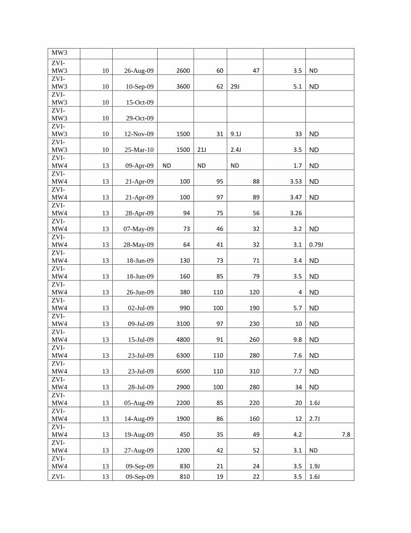
MW3
ZVI-
MW3 10 26-Aug-09 2600 60 47 3.5 ND ZVI-
MW3 10 10-Sep-09 3600 62 29J 5.1 ND
ZVI-
MW3 10 15-Oct-09 ZVI-
MW3 10 29-Oct-09 ZVI-
MW3 10 12-Nov-09 1500 31 9.1J 33 ND
ZVI-
MW3 10 25-Mar-10 1500 21J 2.4J 3.5 ND
ZVI-
MW4 13 09-Apr-09 ND ND ND 1.7 ND
ZVI-
MW4 13 21-Apr-09 100 95 88 3.53 ND
ZVI-
MW4 13 21-Apr-09 100 97 89 3.47 ND
ZVI-
MW4 13 28-Apr-09 94 75 56 3.26 ZVI-
MW4 13 07-May-09 73 46 32 3.2 ND
ZVI-
MW4 13 28-May-09 64 41 32 3.1 0.79J ZVI-
MW4 13 18-Jun-09 130 73 71 3.4 ND
ZVI-
MW4 13 18-Jun-09 160 85 79 3.5 ND
ZVI-
MW4 13 26-Jun-09 380 110 120 4 ND
ZVI-
MW4 13 02-Jul-09 990 100 190 5.7 ND
ZVI-
MW4 13 09-Jul-09 3100 97 230 10 ND
ZVI-
MW4 13 15-Jul-09 4800 91 260 9.8 ND
ZVI-
MW4 13 23-Jul-09 6300 110 280 7.6 ND
ZVI-
MW4 13 23-Jul-09 6500 110 310 7.7 ND
ZVI-
MW4 13 28-Jul-09 2900 100 280 34 ND
ZVI-
MW4 13 05-Aug-09 2200 85 220 20 1.6J ZVI-
MW4 13 14-Aug-09 1900 86 160 12 2.7J ZVI-
MW4 13 19-Aug-09 450 35 49 4.2 7.8 ZVI-
MW4 13 27-Aug-09 1200 42 52 3.1 ND ZVI-
MW4 13 09-Sep-09 830 21 24 3.5 1.9J
ZVI- 13 09-Sep-09 810 19 22 3.5 1.6J
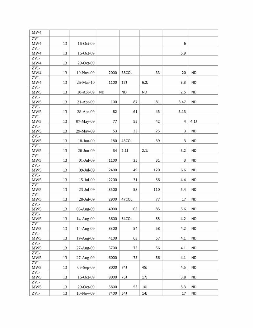
MW4
ZVI-
MW4 13 16-Oct-09 6 ZVI-
MW4 13 16-Oct-09 5.9 ZVI-
MW4 13 29-Oct-09 ZVI-
MW4 13 10-Nov-09 2000 38COL 33 20 ND ZVI-
MW4 13 25-Mar-10 1100 17J 6.2J 3.3 ND ZVI-
MW5 13 10-Apr-09 ND ND ND 2.5 ND ZVI-
MW5 13 21-Apr-09 100 87 81 3.47 ND ZVI-
MW5 13 28-Apr-09 82 61 45 3.13 ZVI-
MW5 13 07-May-09 77 55 42 4 4.1J ZVI-
MW5 13 29-May-09 53 33 25 3 ND ZVI-
MW5 13 18-Jun-09 180 43COL 39 3 ND ZVI-
MW5 13 26-Jun-09 34 2.1J 2.1J 3.2 ND ZVI-
MW5 13 01-Jul-09 1100 25 31 3 ND ZVI-
MW5 13 09-Jul-09 2400 49 120 6.6 ND ZVI-
MW5 13 15-Jul-09 2200 31 56 4.4 ND ZVI-
MW5 13 23-Jul-09 3500 58 110 5.4 ND ZVI-
MW5 13 28-Jul-09 2900 47COL 77 17 ND ZVI-
MW5 13 06-Aug-09 4000 63 85 5.6 ND ZVI-
MW5 13 14-Aug-09 3600 54COL 55 4.2 ND ZVI-
MW5 13 14-Aug-09 3300 54 58 4.2 ND ZVI-
MW5 13 19-Aug-09 4100 63 57 4.1 ND ZVI-
MW5 13 27-Aug-09 5700 73 56 4.1 ND ZVI-
MW5 13 27-Aug-09 6000 75 56 4.1 ND ZVI-
MW5 13 09-Sep-09 8000 74J 45J 4.5 ND ZVI-
MW5 13 16-Oct-09 8000 75J 17J 3.8 ND ZVI-
MW5 13 29-Oct-09 5800 53 10J 5.3 ND
ZVI- 13 10-Nov-09 7400 54J 14J 17 ND

MW5
ZVI-
MW5 13 25-Mar-10 1200 14J 2.4J 2.8 ND ZVI-
MW6 13 13-Apr-09 0.95 ND ND 2.2 ND ZVI-
MW6 13 21-Apr-09 130 100 93 3.19 ND ZVI-
MW6 13 28-Apr-09 100 58 41 3 ZVI-
MW6 13 07-May-09 58 34 24 3.3 ND ZVI-
MW6 13 28-May-09 30 3.7J 3.4J 2.6 0.63J ZVI-
MW6 13 18-Jun-09 37 11COL 11 2.6 ND ZVI-
MW6 13 26-Jun-09 500 31COL 34 3 ND ZVI-
MW6 13 01-Jul-09 510 31 44 3.4 ND ZVI-
MW6 13 10-Jul-09 1600 26 44 5.2 ND ZVI-
MW6 13 10-Jul-09 1600 27COL 45 0.96 ND ZVI-
MW6 13 15-Jul-09 1700 26 45 5.8 ND ZVI-
MW6 13 23-Jul-09 3500 62 97 4.4 ND ZVI-
MW6 13 28-Jul-09 1600 46 100 9.7 ND ZVI-
MW6 13 06-Aug-09 4000 72COL 96 6.2 ND ZVI-
MW6 13 14-Aug-09 4500 63 64 4.6 ND ZVI-
MW6 13 20-Aug-09 6600 62 52 3.7 ND ZVI-
MW6 13 27-Aug-09 8100 68J 56J 3.8 ND ZVI-
MW6 13 10-Sep-09 7200 58J 41J 4.2 ND ZVI-
MW6 13 15-Oct-09 8800 ND 150 3.3 ND ZVI-
MW6 13 29-Oct-09 9000 94J 82J 8.9 ND ZVI-
MW6 13 10-Nov-09 4400 88 48J 21 ND ZVI-
MW6 13 26-Mar-10 490H 4.4JH 22H 2.9 ND ZVI-
MW7 13 13-Apr-09 ND ND ND 2.3 ND ZVI-
MW7 13 13-Apr-09
ND 2.3 ZVI-
MW7 13 13-Apr-09 ND ND ND ND
ZVI- 13 22-Apr-09 80 67 52 2.84 ND

MW7
ZVI-
MW7 13 28-Apr-09 64 33 22 2.89 ZVI-
MW7 13 07-May-09 59 15 10 2.7 ND ZVI-
MW7 13 29-May-09 95 3.6J 3.3J 2.6 ND ZVI-
MW7 13 29-May-09 93 3.3J 3.2J 2.8 ND ZVI-
MW7 13 18-Jun-09 150 15 13 2.6 ND ZVI-
MW7 13 26-Jun-09 270 24 21 2.7 ND ZVI-
MW7 13 26-Jun-09 250 23 20 2.6 ND ZVI-
MW7 13 02-Jul-09 330 18 18 2.6 ND ZVI-
MW7 13 10-Jul-09 2400 27 37 2.4 ND ZVI-
MW7 13 15-Jul-09 840 15 32 3.1 1.6J ZVI-
MW7 13 24-Jul-09 1700 19JCOL 27 3.5 ND ZVI-
MW7 13 28-Jul-09 2200 23J 33 3.2 ND ZVI-
MW7 13 06-Aug-09 3800 46J 45J 3.4 ND ZVI-
MW7 13 14-Aug-09 2400 31 26 2.8 ND ZVI-
MW7 13 19-Aug-09 1800 25JCOL 17J 2.6 ND ZVI-
MW7 13 26-Aug-09 1700 25COL 14J 2.3 ND ZVI-
MW7 13 10-Sep-09 2600 37J 18J 2.5 ND ZVI-
MW7 13 16-Oct-09 1700 24J 6.3J 2.4 ND ZVI-
MW7 13 29-Oct-09 3600 38J 10J 4.2 ND ZVI-
MW7 13 29-Oct-09 3400 40J 11J 4.2 ND ZVI-
MW7 13 12-Nov-09 3400 56 18J 8.3 ND ZVI-
MW7 13 26-Mar-10 65Hp ND ND 2.5 ND ZVI-
MW8 13 10-Apr-09 ND ND ND 2.4 ND ZVI-
MW8 13 21-Apr-09 47 30 22 2.79 ND ZVI-
MW8 13 28-Apr-09 33 9.5 5.8 2.79 ZVI-
MW8 13 07-May-09 43 6.3 4.2J 2.7 ND
ZVI- 13 28-May-09 73 ND ND 2.5 ND

MW8
ZVI-
MW8 13 18-Jun-09 150 0.43 0.67JCOL 2.4 ND ZVI-
MW8 13 26-Jun-09 160 1.2JCOL 1.3J 2.4 ND ZVI-
MW8 13 01-Jul-09 99 0.8JCOL 0.91J 2.2 ND ZVI-
MW8 13 09-Jul-09 0.54JCHI ND 2.3 ND ZVI-
MW8 13 15-Jul-09 0.94JCHI ND 2.2 ND ZVI-
MW8 13 23-Jul-09 23 1J 1.7J 3.1 ND ZVI-
MW8 13 28-Jul-09 18 ND 3 ND ZVI-
MW8 13 06-Aug-09 130 1.3H 0.66J 3.2 ND ZVI-
MW8 13 06-Aug-09 130 1JCOL ND 3.1 ND ZVI-
MW8 13 14-Aug-09 100 0.43J ND 2.7 ND ZVI-
MW8 13 19-Aug-09 39 0.39 ND 2.6 ND ZVI-
MW8 13 26-Aug-09 360 5.8 3.5J 2.3 ND ZVI-
MW8 13 10-Sep-09 380 6.1 3.1J 2.4 ND ZVI-
MW8 13 16-Oct-09 2.7JCOL ND ND 2.3 ND ZVI-
MW8 13 29-Oct-09 610 ND ND 3.1 ND ZVI-
MW8 13 12-Nov-09 6.4COL ND ND 5.7 ND ZVI-
MW8 13 25-Mar-10 630 ND ND 2.4 ND ZVI-
MW9 13 13-Apr-09 ND ND ND 2.2 ND ZVI-
MW9 13 22-Apr-09 ND ND ND 2.6 ND ZVI-
MW9 13 28-Apr-09 2.67 ZVI-
MW9 13 07-May-09 ND ND ND 2.6 ND ZVI-
MW9 13 28-May-09 ND ND ND 2.4 ND ZVI-
MW9 13 18-Jun-09 0.97J ND ND 2.6B ND ZVI-
MW9 13 26-Jun-09 303J ND ND 3.1 ND ZVI-
MW9 13 02-Jul-09 2.9J ND ND 2.5 ND ZVI-
MW9 13 10-Jul-09 0.66JCHI ND ND 2.3 ND
ZVI- 13 15-Jul-09 ND ND ND 2.2 ND
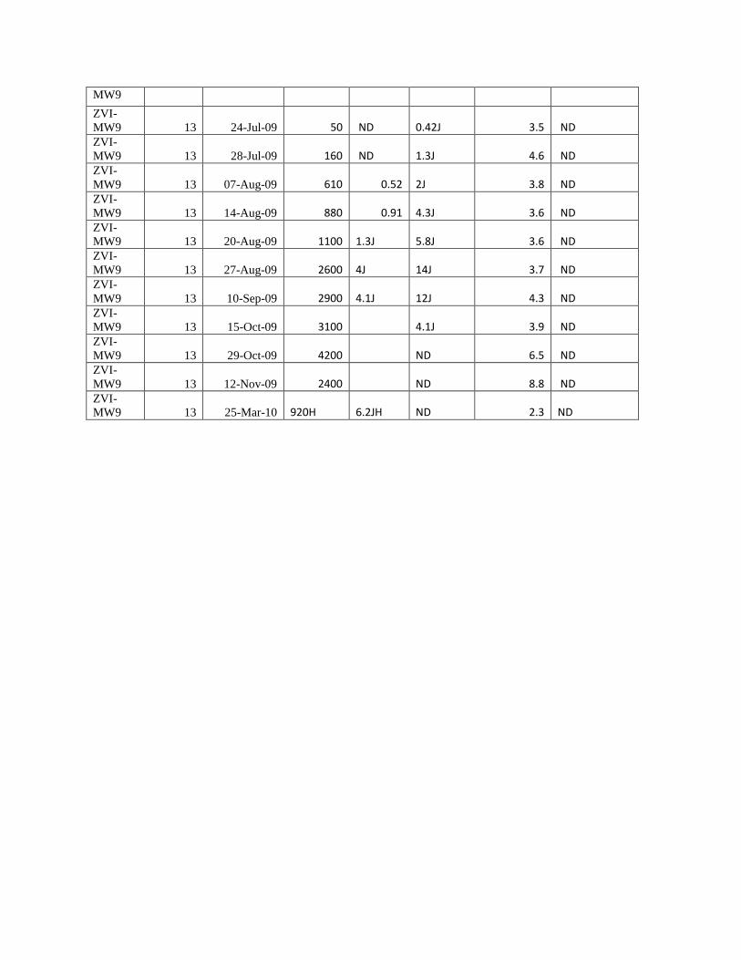
MW9
ZVI-
MW9 13 24-Jul-09 50 ND 0.42J 3.5 ND ZVI-
MW9 13 28-Jul-09 160 ND 1.3J 4.6 ND ZVI-
MW9 13 07-Aug-09 610 0.52 2J 3.8 ND ZVI-
MW9 13 14-Aug-09 880 0.91 4.3J 3.6 ND ZVI-
MW9 13 20-Aug-09 1100 1.3J 5.8J 3.6 ND ZVI-
MW9 13 27-Aug-09 2600 4J 14J 3.7 ND ZVI-
MW9 13 10-Sep-09 2900 4.1J 12J 4.3 ND ZVI-
MW9 13 15-Oct-09 3100
4.1J 3.9 ND ZVI-
MW9 13 29-Oct-09 4200
ND 6.5 ND ZVI-
MW9 13 12-Nov-09 2400
ND 8.8 ND ZVI-
MW9 13 25-Mar-10 920H 6.2JH ND 2.3 ND

Table 8. ZVI Analytical Results Redox Parameters
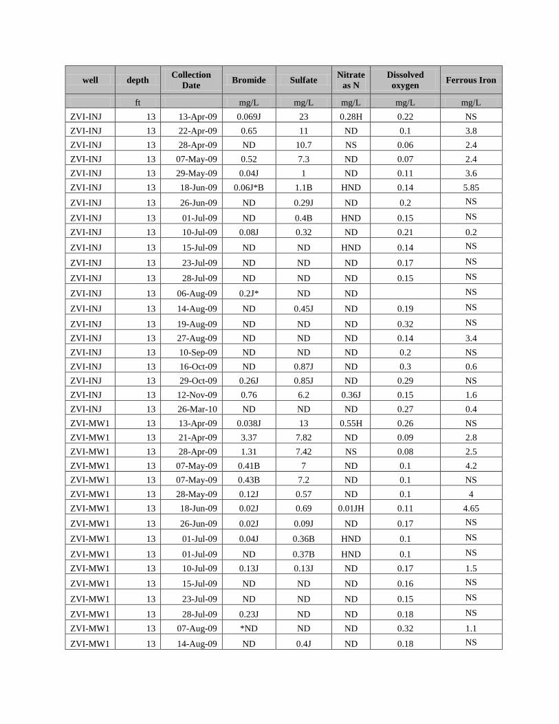
well depth Collection
Date Bromide Sulfate
Nitrate
as N
Dissolved
oxygen Ferrous Iron
ft mg/L mg/L mg/L mg/L mg/L
ZVI-INJ 13 13-Apr-09 0.069J 23 0.28H 0.22 NS
ZVI-INJ 13 22-Apr-09 0.65 11 ND 0.1 3.8
ZVI-INJ 13 28-Apr-09 ND 10.7 NS 0.06 2.4
ZVI-INJ 13 07-May-09 0.52 7.3 ND 0.07 2.4
ZVI-INJ 13 29-May-09 0.04J 1 ND 0.11 3.6
ZVI-INJ 13 18-Jun-09 0.06J*B 1.1B HND 0.14 5.85
ZVI-INJ 13 26-Jun-09 ND 0.29J ND 0.2 NS
ZVI-INJ 13 01-Jul-09 ND 0.4B HND 0.15 NS
ZVI-INJ 13 10-Jul-09 0.08J 0.32 ND 0.21 0.2
ZVI-INJ 13 15-Jul-09 ND ND HND 0.14 NS
ZVI-INJ 13 23-Jul-09 ND ND ND 0.17 NS
ZVI-INJ 13 28-Jul-09 ND ND ND 0.15 NS
ZVI-INJ 13 06-Aug-09 0.2J* ND ND
NS
ZVI-INJ 13 14-Aug-09 ND 0.45J ND 0.19 NS
ZVI-INJ 13 19-Aug-09 ND ND ND 0.32 NS
ZVI-INJ 13 27-Aug-09 ND ND ND 0.14 3.4
ZVI-INJ 13 10-Sep-09 ND ND ND 0.2 NS
ZVI-INJ 13 16-Oct-09 ND 0.87J ND 0.3 0.6
ZVI-INJ 13 29-Oct-09 0.26J 0.85J ND 0.29 NS
ZVI-INJ 13 12-Nov-09 0.76 6.2 0.36J 0.15 1.6
ZVI-INJ 13 26-Mar-10 ND ND ND 0.27 0.4
ZVI-MW1 13 13-Apr-09 0.038J 13 0.55H 0.26 NS
ZVI-MW1 13 21-Apr-09 3.37 7.82 ND 0.09 2.8
ZVI-MW1 13 28-Apr-09 1.31 7.42 NS 0.08 2.5
ZVI-MW1 13 07-May-09 0.41B 7 ND 0.1 4.2
ZVI-MW1 13 07-May-09 0.43B 7.2 ND 0.1 NS
ZVI-MW1 13 28-May-09 0.12J 0.57 ND 0.1 4
ZVI-MW1 13 18-Jun-09 0.02J 0.69 0.01JH 0.11 4.65
ZVI-MW1 13 26-Jun-09 0.02J 0.09J ND 0.17 NS
ZVI-MW1 13 01-Jul-09 0.04J 0.36B HND 0.1 NS
ZVI-MW1 13 01-Jul-09 ND 0.37B HND 0.1 NS
ZVI-MW1 13 10-Jul-09 0.13J 0.13J ND 0.17 1.5
ZVI-MW1 13 15-Jul-09 ND ND ND 0.16 NS
ZVI-MW1 13 23-Jul-09 ND ND ND 0.15 NS
ZVI-MW1 13 28-Jul-09 0.23J ND ND 0.18 NS
ZVI-MW1 13 07-Aug-09 *ND ND ND 0.32 1.1
ZVI-MW1 13 14-Aug-09 ND 0.4J ND 0.18 NS

ZVI-MW1 13 20-Aug-09 ND ND ND 0.2 NS
ZVI-MW1 13 20-Aug-09 ND ND ND 0.2 NS
ZVI-MW1 13 26-Aug-09 ND ND HND 0.32 0.8
ZVI-MW1 13 10-Sep-09 ND ND ND 0.35 NS
ZVI-MW1 13 16-Oct-09 ND ND ND 1.82 NS
ZVI-MW1 13 29-Oct-09 ND ND ND 0.63 NS
ZVI-MW1 13 10-Nov-09 0.64 13 0.32J 0.23 2.5
ZVI-MW1 13 10-Nov-09 0.66 13 0.3J 0.23 NS
ZVI-MW1 13 26-Mar-10 ND 4.6 ND 0.31 3
ZVI-MW1 13 26-Mar-10 ND 5 ND 0.31 3
ZVI-MW2 13 09-Apr-09 ND ND 1.2 0.32 NS
ZVI-MW2 13 21-Apr-09 0.46 9.38 ND 0.19 NS
ZVI-MW2 13 28-Apr-09 ND 9.23 NS 0.18 3
ZVI-MW2 13 07-May-09 0.04JB 8.1 ND 0.1 2.6
ZVI-MW2 13 28-May-09 0.02J 0.8 ND 0.36 3.8
ZVI-MW2 13 18-Jun-09 ND 0.85 HND 0.19 4.4
ZVI-MW2 13 26-Jun-09 0.05J 0.07J ND 0.24 NS
ZVI-MW2 13 02-Jul-09 ND 0.27JB HND 0.25 NS
ZVI-MW2 13 09-Jul-09 0.03J 2.4 ND 0.27 3.3
ZVI-MW2 13 15-Jul-09 ND 7.8 ND 0.22 NS
ZVI-MW2 13 15-Jul-09 ND 8.2 ND 0.22 NS
ZVI-MW2 13 23-Jul-09 ND 1.3 ND 0.21 NS
ZVI-MW2 13 28-Jul-09 ND ND ND 0.26 NS
ZVI-MW2 13 05-Aug-09 *ND ND HND 0.46 2.8
ZVI-MW2 13 14-Aug-09 ND 2.2 ND 0.25 NS
ZVI-MW2 13 19-Aug-09 ND 1.9 ND 0.27 NS
ZVI-MW2 13 26-Aug-09 ND 1.4 HND 0.27 2.9
ZVI-MW2 13 09-Sep-09 ND 4.5 ND 0.44 NS
ZVI-MW2 13 16-Oct-09 ND 6.8 ND 0.67 1
ZVI-MW2 13 29-Oct-09 ND 26 ND 0.39 NS
ZVI-MW2 13 10-Nov-09 ND 23 2.8 0.33 0.8
ZVI-MW2 13 25-Mar-10 ND 8.7 ND 0.3 2.6
ZVI-MW3 10 10-Apr-09 ND NS 1.2 0.29 NS
ZVI-MW3 10 21-Apr-09 1.06 9.57 ND 0.18 3.8
ZVI-MW3 10 28-Apr-09 ND 9.46 NS 0.11 4
ZVI-MW3 10 28-Apr-09 ND 9.43 NS 0.11 NS
ZVI-MW3 10 07-May-09 0.25B 6.6 ND 0.12 3.4
ZVI-MW3 10 29-May-09 0.02J 0.18J ND 0.22 3.8
ZVI-MW3 10 18-Jun-09 0.39 0.07J HND 0.14 4.5
ZVI-MW3 10 26-Jun-09 ND 0.11J ND 0.27 NS

ZVI-MW3 10 01-Jul-09 ND 0.43B HND 0.21 NS
ZVI-MW3 10 09-Jul-09 0.16 0.78 ND 0.24 2.9
ZVI-MW3 10 15-Jul-09 ND 2.8 ND 0.23 NS
ZVI-MW3 10 23-Jul-09 ND 0.71J ND 0.35 NS
ZVI-MW3 10 28-Jul-09 0.38J 7.6 ND 0.24 NS
ZVI-MW3 10 28-Jul-09 ND 7.5 ND 0.24 NS
ZVI-MW3 10 06-Aug-09 *ND 0.45J ND 0.57 3.5
ZVI-MW3 10 14-Aug-09 ND 1.7 ND 0.83 NS
ZVI-MW3 10 19-Aug-09 ND 0.45J ND 0.39 NS
ZVI-MW3 10 26-Aug-09 ND 0.47J HND 0.99 2
ZVI-MW3 10 10-Sep-09 ND 1.7 ND 3.14 NS
ZVI-MW3 10 15-Oct-09 NS NS NS NA NS
ZVI-MW3 10 29-Oct-09 NS NS NS NA NS
ZVI-MW3 10 12-Nov-09 0.59J 48 2.4 0.94 0.8
ZVI-MW3 10 25-Mar-10 ND 11 ND 0.35 2.6
ZVI-MW4 13 09-Apr-09 ND NS 1.2 0.25 NS
ZVI-MW4 13 21-Apr-09 1.58 10.5 ND 0.08 3.8
ZVI-MW4 13 28-Apr-09 0.47 9.45 NS 0.06 2.6
ZVI-MW4 13 07-May-09 0.31B 7.5 ND 0.12 4.2
ZVI-MW4 13 28-May-09 0.1J 0.73 ND 0.08 4.4
ZVI-MW4 13 18-Jun-09 ND 0.09J HND 0.15 2.8
ZVI-MW4 13 18-Jun-09 0.02J 0.59 HND 0.15 NS
ZVI-MW4 13 26-Jun-09 0.33 0.06J 0.01J 0.2 NS
ZVI-MW4 13 02-Jul-09 ND 0.34B HND 0.19 NS
ZVI-MW4 13 09-Jul-09 0.22 0.09J 0.07 0.2 3
ZVI-MW4 13 15-Jul-09 ND ND ND 0.11 NS
ZVI-MW4 13 23-Jul-09 ND ND ND 0.19 NS
ZVI-MW4 13 23-Jul-09 ND ND ND 0.19 NS
ZVI-MW4 13 28-Jul-09 ND ND ND 0.18 NS
ZVI-MW4 13 05-Aug-09 0.24J* ND HND 0.32 4.5
ZVI-MW4 13 14-Aug-09 0.29J ND ND 0.23 NS
ZVI-MW4 13 19-Aug-09 ND ND ND 0.15 NS
ZVI-MW4 13 27-Aug-09 ND ND ND 0.27 2.9
ZVI-MW4 13 09-Sep-09 ND ND ND 0.98 NS
ZVI-MW4 13 09-Sep-09 ND ND ND 0.98 NS
ZVI-MW4 13 16-Oct-09 ND 1.5 ND 0.83 NS
ZVI-MW4 13 16-Oct-09 ND 1.4 ND 0.83 NS
ZVI-MW4 13 29-Oct-09 NS NS ND 0.42 NS
ZVI-MW4 13 10-Nov-09 0.41J 6.5 ND 1.71 2.4

ZVI-MW4 13 25-Mar-10 ND 9.3 ND 0.39 2.8
ZVI-MW5 13 10-Apr-09 0.022J NS 1.1 0.33 NS
ZVI-MW5 13 21-Apr-09 2.14 10.7 ND 0.15 3
ZVI-MW5 13 28-Apr-09 ND 9.22 NS 0.16 3
ZVI-MW5 13 07-May-09 0.38B 8.8 ND 0.12 7
ZVI-MW5 13 29-May-09 0.06J 0.42 ND 0.21 4.6
ZVI-MW5 13 18-Jun-09 ND 0.33 HND 0.22 3.2
ZVI-MW5 13 26-Jun-09 0.09J 0.5 ND 0.31 NS
ZVI-MW5 13 01-Jul-09 ND 0.66B HND 0.23 NS
ZVI-MW5 13 09-Jul-09 0.14J 0.96 ND 0.27 4
ZVI-MW5 13 15-Jul-09 ND 1.9 HND 0.27 NS
ZVI-MW5 13 23-Jul-09 ND 0.53J ND 0.38 NS
ZVI-MW5 13 28-Jul-09 0.2J 0.99J ND 0.31 NS
ZVI-MW5 13 06-Aug-09 *ND 0.49J ND 0.33 3
ZVI-MW5 13 14-Aug-09 ND 0.51J ND 0.36 NS
ZVI-MW5 13 14-Aug-09 ND 0.65J ND 0.36 NS
ZVI-MW5 13 19-Aug-09 0.28J ND ND 0.34 NS
ZVI-MW5 13 27-Aug-09 ND ND ND 0.44 2.4
ZVI-MW5 13 27-Aug-09 ND ND ND 0.44 NS
ZVI-MW5 13 09-Sep-09 ND ND ND 0.47 NS
ZVI-MW5 13 16-Oct-09 ND 1.5 ND 0.5 2.3
ZVI-MW5 13 29-Oct-09 ND 8.4 ND 0.49 NS
ZVI-MW5 13 10-Nov-09 0.49J 9.1 0.34 0.33 2.8
ZVI-MW5 13 25-Mar-10 ND 10 ND 0.39 2.8
ZVI-MW6 13 13-Apr-09 0.039J 10 0.72 0.15 NS
ZVI-MW6 13 21-Apr-09 2.51 9.92 ND 0.1 2.8
ZVI-MW6 13 28-Apr-09 0.44 9.41 NS 0.11 2.8
ZVI-MW6 13 07-May-09 0.27B 8.9 ND 0.1 3.6
ZVI-MW6 13 28-May-09 0.14J 4.4 ND 0.13 4.5
ZVI-MW6 13 18-Jun-09 ND 4.7 HND 0.26 3
ZVI-MW6 13 26-Jun-09 ND 2.7 ND 0.27 NS
ZVI-MW6 13 01-Jul-09 ND 2.3B HND 0.18 NS
ZVI-MW6 13 10-Jul-09 0.14J 2.2 ND 0.23 3.5
ZVI-MW6 13 10-Jul-09 ND 0.4 ND 0.23 NS
ZVI-MW6 13 15-Jul-09 ND 3.2 HND 0.15 NS
ZVI-MW6 13 23-Jul-09 ND ND ND 0.21 NS
ZVI-MW6 13 28-Jul-09 0.36J 0.52J ND 0.3 NS
ZVI-MW6 13 06-Aug-09 *ND ND ND 0.27 3.8
ZVI-MW6 13 14-Aug-09 ND ND ND 0.24 NS
ZVI-MW6 13 20-Aug-09 ND 3.6 ND 0.27 NS

ZVI-MW6 13 27-Aug-09 ND 1.1J ND 0.24 2.8
ZVI-MW6 13 10-Sep-09 ND ND ND 0.34 NS
ZVI-MW6 13 15-Oct-09 ND ND ND 0.33 0.6
ZVI-MW6 13 29-Oct-09 ND 2 ND 0.33 NS
ZVI-MW6 13 10-Nov-09 0.69 26 0.91 0.2 2.6
ZVI-MW6 13 26-Mar-10 ND 3.5 ND 0.3 2.6
ZVI-MW7 13 13-Apr-09 0.027J 10 0.88H 0.32 NS
ZVI-MW7 13 13-Apr-09 0.029J 10 0.87H 0.32 NS
ZVI-MW7 13 22-Apr-09 ND 9.48 ND 0.18 2.8
ZVI-MW7 13 28-Apr-09 ND 9.64 NS 0.08 3
ZVI-MW7 13 07-May-09 0.11JB 8.6 ND 0.09 4
ZVI-MW7 13 29-May-09 0.12J 2.1 ND 0.1 2.2
ZVI-MW7 13 29-May-09 0.11JB 2 0.03J 0.1 NS
ZVI-MW7 13 18-Jun-09 ND 2.3 HND 0.33 3
ZVI-MW7 13 26-Jun-09 ND 1.8 ND 0.4 NS
ZVI-MW7 13 26-Jun-09 ND 1.5 ND 0.4 NS
ZVI-MW7 13 02-Jul-09 ND 0.81B HND 0.18 NS
ZVI-MW7 13 10-Jul-09 ND 2.5 0.03J 0.18 2.4
ZVI-MW7 13 15-Jul-09 ND 8.6 HND 0.21 NS
ZVI-MW7 13 24-Jul-09 ND 1J ND 0.42 NS
ZVI-MW7 13 28-Jul-09 ND 0.51J ND 0.27 NS
ZVI-MW7 13 06-Aug-09 *ND 1J ND 0.41 3
ZVI-MW7 13 14-Aug-09 ND 2.9 ND 0.51 NS
ZVI-MW7 13 19-Aug-09 ND 6.7 ND 0.37 NS
ZVI-MW7 13 26-Aug-09 ND 3.7 HND 0.37 2.2
ZVI-MW7 13 10-Sep-09 ND 2.8 ND 0.42 NS
ZVI-MW7 13 16-Oct-09 ND 6.2 ND 0.34 3.8
ZVI-MW7 13 29-Oct-09 ND 15 ND 0.38 NS
ZVI-MW7 13 29-Oct-09 ND 15 ND 0.38 NS
ZVI-MW7 13 12-Nov-09 ND 20 0.42J 0.36 3.2
ZVI-MW7 13 26-Mar-10 ND 14 ND 0.34 2.8
ZVI-MW8 13 10-Apr-09 ND NS 1.1 0.31 NS
ZVI-MW8 13 21-Apr-09 ND 9.9 ND 0.25 2.8
ZVI-MW8 13 28-Apr-09 ND 9.61 NS 0.25 3
ZVI-MW8 13 07-May-09 0.2B 10 0.01J 0.25 4
ZVI-MW8 13 28-May-09 ND 9.3 0.16 0.19 0.03
ZVI-MW8 13 18-Jun-09 ND 8 0.01JH 0.25 1.5
ZVI-MW8 13 26-Jun-09 ND 7.4 0.01J 0.38 NS
ZVI-MW8 13 01-Jul-09 ND 6.6B HND 0.6 NS
ZVI-MW8 13 09-Jul-09 0.15 7.8 0.56 2.53 0.2

ZVI-MW8 13 15-Jul-09 0.27J 8.3 0.61JH 3.79 NS
ZVI-MW8 13 23-Jul-09 ND 6.6 ND 0.6 NS
ZVI-MW8 13 28-Jul-09 ND 7.2 ND 0.8 NS
ZVI-MW8 13 06-Aug-09 *ND 3.9 ND 0.75 2.8
ZVI-MW8 13 06-Aug-09 *ND 3.7 ND 0.75 NS
ZVI-MW8 13 14-Aug-09 ND 5.5 ND 0.36 NS
ZVI-MW8 13 19-Aug-09 ND 6.7 ND 0.34 NS
ZVI-MW8 13 26-Aug-09 ND 5.3 HND 0.35 2.2
ZVI-MW8 13 10-Sep-09 ND 5.4 ND 0.7 NS
ZVI-MW8 13 16-Oct-09 ND 7.3 ND 0.79 NS
ZVI-MW8 13 29-Oct-09 ND 2.5 0.38J 0.42 NS
ZVI-MW8 13 12-Nov-09 0.4J 18 5.7 0.75 0
ZVI-MW8 13 25-Mar-10 ND 18 ND 0.33 2.1
ZVI-MW9 13 13-Apr-09 0.026J 10 0.9H 0.92 NS
ZVI-MW9 13 22-Apr-09 ND 10.1 0.96 0.9 0.1
ZVI-MW9 13 28-Apr-09 ND 10.1 NS 0.98 0
ZVI-MW9 13 07-May-09 0.19 11 0.59 0.71 0.2
ZVI-MW9 13 28-May-09 ND 9.9 0.43 0.82 0
ZVI-MW9 13 18-Jun-09 *ND 9.7B 0.13HB 0.18 0.25
ZVI-MW9 13 26-Jun-09 0.08J 0.09J 0.21 0.36 NS
ZVI-MW9 13 02-Jul-09 ND 8B 0.2H 0.35 NS
ZVI-MW9 13 10-Jul-09 ND 7.8 0.41 2.35 0.2
ZVI-MW9 13 15-Jul-09 ND 8.2 0.42JH 2.83 NS
ZVI-MW9 13 24-Jul-09 ND 6.4 ND 0.37 NS
ZVI-MW9 13 28-Jul-09 ND 1.5 ND 0.27 NS
ZVI-MW9 13 07-Aug-09 *ND 2.7 HND 0.43 4.4
ZVI-MW9 13 14-Aug-09 ND 2.2 ND 0.34 NS
ZVI-MW9 13 20-Aug-09 0.22J 3.7 ND 0.32 NS
ZVI-MW9 13 27-Aug-09 ND 0.95J ND 0.29 4.4
ZVI-MW9 13 10-Sep-09 ND 0.76J ND 0.2 NS
ZVI-MW9 13 15-Oct-09 0.22J 1.7 ND 0.38 3
ZVI-MW9 13 29-Oct-09 0.26J 0.41J ND 0.35 NS
ZVI-MW9 13 12-Nov-09 0.33J 19 ND 0.55 3.4
ZVI-MW9 13 25-Mar-10 ND 10 0.54J 0.61 0

Table 9. ZVI Analytical Results Chlorinated Ethenes

well depth Collection
Date PCE TCE
cis-1,2-
DCE
trans-
1,2-DCE
Vinyl
chloride
ft ug/L ug/L ug/L ug/L ug/L
ZVI-INJ 13 13-Apr-09 5.5 25000B 3200 22 2.8
ZVI-INJ 13 22-Apr-09 1.5 810 88 1.3 ND
ZVI-INJ 13 28-Apr-09 0.99J 580 300 2J 0.9J
ZVI-INJ 13 07-May-09 0.28JND 260 380 1.9 2
ZVI-INJ 13 29-May-09 ND 38 470 1.5 2
ZVI-INJ 13 18-Jun-09 0.19J 51 1200 8 4
ZVI-INJ 13 26-Jun-09 0.19J 39 420 2.5 2.1
ZVI-INJ 13 01-Jul-09 HND 73H 850H .95JH 2.6H
ZVI-INJ 13 10-Jul-09 ND 100 550 1.2 1.6
ZVI-INJ 13 15-Jul-09 0.15J 85 480 20 1.7
ZVI-INJ 13 23-Jul-09 0.39JB 170 820 2.6 1.1
ZVI-INJ 13 28-Jul-09 0.35J 110 740 2.7 0.87J
ZVI-INJ 13 06-Aug-09 0.47J 150 900 2.1 0.24J
ZVI-INJ 13 14-Aug-09 0.97J 400 1000 3.6 ND
ZVI-INJ 13 19-Aug-09 0.78J 160 430 2 ND
ZVI-INJ 13 27-Aug-09 0.72J 170 380 1.5 ND
ZVI-INJ 13 10-Sep-09 0.72J 150 320 .86J ND
ZVI-INJ 13 16-Oct-09 0.52J 110 180 ND ND
ZVI-INJ 13 29-Oct-09 0.42J 140 370 ND 0.68J
ZVI-INJ 13 12-Nov-09 0.41J 130 620 0.44J 1
ZVI-INJ 13 26-Mar-10 0.27J 27 1400 0.37J 2.9
ZVI-MW1 13 13-Apr-09 0.21J 140B 69B 1 ND
ZVI-MW1 13 21-Apr-09 0.89 650 410 5 ND
ZVI-MW1 13 28-Apr-09 0.56J 150 770 6.6 ND
ZVI-MW1 13 07-May-09 ND 11 140 0.94J 1.3
ZVI-MW1 13 07-May-09 ND 9.4 76 0.68J 1.2
ZVI-MW1 13 28-May-09 ND 10 330 1.2 1J
ZVI-MW1 13 18-Jun-09 ND 9.1 340 3.1 1.2
ZVI-MW1 13 26-Jun-09 ND 4.9 170 1.7 1.7
ZVI-MW1 13 01-Jul-09 HND 25 1000 1.4H 3.3H
ZVI-MW1 13 01-Jul-09 HND 24 930 1.5H 3.3H
ZVI-MW1 13 10-Jul-09 ND 27 600 1.9 2.5
ZVI-MW1 13 15-Jul-09 ND 20 640 22 1.3
ZVI-MW1 13 23-Jul-09 0.089JB 34 710 1.9 0.77J
ZVI-MW1 13 28-Jul-09 ND 30 510 1.6 0.35J
ZVI-MW1 13 07-Aug-09 0.19J 110 530 1.3 0.29J
ZVI-MW1 13 14-Aug-09 0.28J 250 520 1.9 0.19J
ZVI-MW1 13 20-Aug-09 0.31J 380 190 1.2 ND
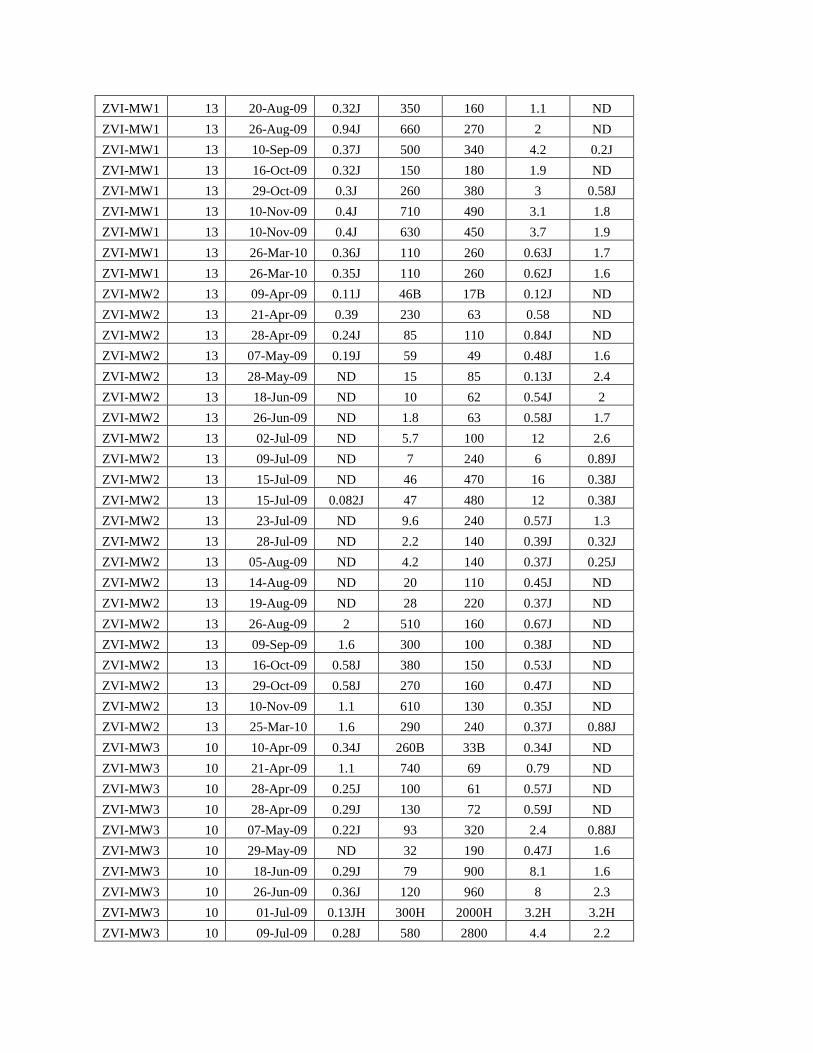
ZVI-MW1 13 20-Aug-09 0.32J 350 160 1.1 ND
ZVI-MW1 13 26-Aug-09 0.94J 660 270 2 ND
ZVI-MW1 13 10-Sep-09 0.37J 500 340 4.2 0.2J
ZVI-MW1 13 16-Oct-09 0.32J 150 180 1.9 ND
ZVI-MW1 13 29-Oct-09 0.3J 260 380 3 0.58J
ZVI-MW1 13 10-Nov-09 0.4J 710 490 3.1 1.8
ZVI-MW1 13 10-Nov-09 0.4J 630 450 3.7 1.9
ZVI-MW1 13 26-Mar-10 0.36J 110 260 0.63J 1.7
ZVI-MW1 13 26-Mar-10 0.35J 110 260 0.62J 1.6
ZVI-MW2 13 09-Apr-09 0.11J 46B 17B 0.12J ND
ZVI-MW2 13 21-Apr-09 0.39 230 63 0.58 ND
ZVI-MW2 13 28-Apr-09 0.24J 85 110 0.84J ND
ZVI-MW2 13 07-May-09 0.19J 59 49 0.48J 1.6
ZVI-MW2 13 28-May-09 ND 15 85 0.13J 2.4
ZVI-MW2 13 18-Jun-09 ND 10 62 0.54J 2
ZVI-MW2 13 26-Jun-09 ND 1.8 63 0.58J 1.7
ZVI-MW2 13 02-Jul-09 ND 5.7 100 12 2.6
ZVI-MW2 13 09-Jul-09 ND 7 240 6 0.89J
ZVI-MW2 13 15-Jul-09 ND 46 470 16 0.38J
ZVI-MW2 13 15-Jul-09 0.082J 47 480 12 0.38J
ZVI-MW2 13 23-Jul-09 ND 9.6 240 0.57J 1.3
ZVI-MW2 13 28-Jul-09 ND 2.2 140 0.39J 0.32J
ZVI-MW2 13 05-Aug-09 ND 4.2 140 0.37J 0.25J
ZVI-MW2 13 14-Aug-09 ND 20 110 0.45J ND
ZVI-MW2 13 19-Aug-09 ND 28 220 0.37J ND
ZVI-MW2 13 26-Aug-09 2 510 160 0.67J ND
ZVI-MW2 13 09-Sep-09 1.6 300 100 0.38J ND
ZVI-MW2 13 16-Oct-09 0.58J 380 150 0.53J ND
ZVI-MW2 13 29-Oct-09 0.58J 270 160 0.47J ND
ZVI-MW2 13 10-Nov-09 1.1 610 130 0.35J ND
ZVI-MW2 13 25-Mar-10 1.6 290 240 0.37J 0.88J
ZVI-MW3 10 10-Apr-09 0.34J 260B 33B 0.34J ND
ZVI-MW3 10 21-Apr-09 1.1 740 69 0.79 ND
ZVI-MW3 10 28-Apr-09 0.25J 100 61 0.57J ND
ZVI-MW3 10 28-Apr-09 0.29J 130 72 0.59J ND
ZVI-MW3 10 07-May-09 0.22J 93 320 2.4 0.88J
ZVI-MW3 10 29-May-09 ND 32 190 0.47J 1.6
ZVI-MW3 10 18-Jun-09 0.29J 79 900 8.1 1.6
ZVI-MW3 10 26-Jun-09 0.36J 120 960 8 2.3
ZVI-MW3 10 01-Jul-09 0.13JH 300H 2000H 3.2H 3.2H
ZVI-MW3 10 09-Jul-09 0.28J 580 2800 4.4 2.2
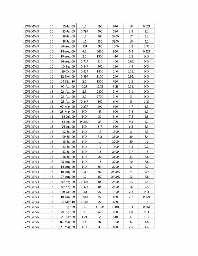
ZVI-MW3 10 15-Jul-09 1.6 690 670 16 0.62J
ZVI-MW3 10 23-Jul-09 0.79J 500 590 1.8 1.2
ZVI-MW3 10 28-Jul-09 1.6 760 3800 17 5.2
ZVI-MW3 10 28-Jul-09 1.5 830 3900 16 5.2
ZVI-MW3 10 06-Aug-09 .43J 580 1000 2.2 0.9J
ZVI-MW3 10 14-Aug-09 6.8 6600 950 5.4 0.52J
ZVI-MW3 10 19-Aug-09 2.6 1500 410 2.2 ND
ZVI-MW3 10 26-Aug-09 0.71J 410 400 0.96J ND
ZVI-MW3 10 10-Sep-09 0.84J 460 130 4.9 ND
ZVI-MW3 10 29-Oct-09 0.82J 1800 240 0.32J ND
ZVI-MW3 10 12-Nov-09 0.89J 1100 260 0.95J ND
ZVI-MW3 10 25-Mar-10 2.6 1300 620 1.2 ND
ZVI-MW4 13 09-Apr-09 0.2J 120B 31B 0.31J ND
ZVI-MW4 13 21-Apr-09 2.5 2800 340 3.1 ND
ZVI-MW4 13 21-Apr-09 3.2 2700 340 3 ND
ZVI-MW4 13 28-Apr-09 0.84J 360 640 5 1.3J
ZVI-MW4 13 07-May-09 0.27J 100 660 4.7 1.5
ZVI-MW4 13 28-May-09 ND 45 990 3.8 1.3
ZVI-MW4 13 18-Jun-09 ND 32 840 7.5 2.8
ZVI-MW4 13 18-Jun-09 0.088J 33 790 9.2 2.1
ZVI-MW4 13 26-Jun-09 ND 8.7 990 6.5 3.3
ZVI-MW4 13 02-Jul-09 ND 15 1800 3 5.5
ZVI-MW4 13 09-Jul-09 ND 3.2 3600 20 8.4
ZVI-MW4 13 15-Jul-09 ND 11 3200 89 12
ZVI-MW4 13 23-Jul-09 ND 17 1600 4.5 9.2
ZVI-MW4 13 23-Jul-09 ND 18 2400 3.7 13
ZVI-MW4 13 28-Jul-09 ND 26 3100 23 6.8
ZVI-MW4 13 05-Aug-09 ND 18 3200 10 8.8
ZVI-MW4 13 14-Aug-09 ND 95 2200 5 8.7
ZVI-MW4 13 19-Aug-09 1.1 860 2800E 14 2.9
ZVI-MW4 13 27-Aug-09 1.2 450 2500E 12 6.8
ZVI-MW4 13 09-Sep-09 0.49J 400 2400 13 2.4
ZVI-MW4 13 09-Sep-09 0.47J 400 2400 16 2.5
ZVI-MW4 13 29-Oct-09 0.5J 950 1300 2.2 ND
ZVI-MW4 13 10-Nov-09 0.68J 850 850 2.7 0.42J
ZVI-MW4 13 25-Mar-10 0.16J 22 630 1 16
ZVI-MW5 13 10-Apr-09 1.6 1100B 100B 1.4 0.45J
ZVI-MW5 13 21-Apr-09 3 2500 450 4.9 ND
ZVI-MW5 13 28-Apr-09 1.2J 620 510 4J 1.1J
ZVI-MW5 13 07-May-09 1J 780 1000 6 1.8
ZVI-MW5 13 29-May-09 ND 35 870 2.5 1.4

ZVI-MW5 13 18-Jun-09 ND 63 280 4.4 1.7
ZVI-MW5 13 26-Jun-09 ND 30 520 3.6 2.4
ZVI-MW5 13 01-Jul-09 HND 51 440 1.1H 2.1H
ZVI-MW5 13 09-Jul-09 ND 59 1700 4.7 4.6
ZVI-MW5 13 15-Jul-09 ND 47 1300 35 2.7
ZVI-MW5 13 23-Jul-09 ND 52 1600 2.6 3.2
ZVI-MW5 13 28-Jul-09 0.15J 89 2400 19 3.2
ZVI-MW5 13 06-Aug-09 0.27J 170 700 1.8 0.97J
ZVI-MW5 13 14-Aug-09 0.53J 640 1200 3.7 0.87J
ZVI-MW5 13 14-Aug-09 0.63J 580 1000 4.8 0.9J
ZVI-MW5 13 19-Aug-09 0.6J 400 1500E 3.5 ND
ZVI-MW5 13 27-Aug-09 2.9 1600 760 4 0.88J
ZVI-MW5 13 27-Aug-09 2.7 1500 710 3.8 0.82J
ZVI-MW5 13 09-Sep-09 1.7 620 450 3.9 0.6J
ZVI-MW5 13 16-Oct-09 0.6J 340 250 3.2 ND
ZVI-MW5 13 29-Oct-09 2 1800 550 4.5 ND
ZVI-MW5 13 10-Nov-09 1.7 1100 400 2 0.42J
ZVI-MW5 13 25-Mar-10 0.41J 160 480 0.74J 2.9
ZVI-MW6 13 13-Apr-09 0.13J 79B 25B 0.39J 0.26J
ZVI-MW6 13 21-Apr-09 0.83 500 240 3.7 ND
ZVI-MW6 13 28-Apr-09 0.39J 98 230 2 3
ZVI-MW6 13 07-May-09 ND 15 200 1.5 2.2
ZVI-MW6 13 28-May-09 ND 39 170 1.3 1.8
ZVI-MW6 13 18-Jun-09 0.069J 39 170 3 2.7
ZVI-MW6 13 26-Jun-09 0.086J 46 440 5.5 7.7
ZVI-MW6 13 01-Jul-09 HND 74H 1200B 4.6H 25H
ZVI-MW6 13 10-Jul-09 ND 36 2000 9.2 28
ZVI-MW6 13 10-Jul-09 ND 35 2100 8.9 27
ZVI-MW6 13 15-Jul-09 ND 29 3100 130 36
ZVI-MW6 13 23-Jul-09 ND 11 1400 5.3 37
ZVI-MW6 13 28-Jul-09 0.11J 72 3100 26 48
ZVI-MW6 13 06-Aug-09 ND 28 690 3.9 12
ZVI-MW6 13 14-Aug-09 ND 32 450 2.7 6.4
ZVI-MW6 13 20-Aug-09 ND 68 190 2.2 3.2
ZVI-MW6 13 27-Aug-09 ND 67 280 3.9 3.1
ZVI-MW6 13 10-Sep-09 ND 68 280 4.5 1.6
ZVI-MW6 13 15-Oct-09 ND 71B 170B 3.4 1.3
ZVI-MW6 13 29-Oct-09 ND 140 350 3.2 1.7
ZVI-MW6 13 10-Nov-09 0.25J 250 250 1.9 1
ZVI-MW6 13 26-Mar-10 0.12J 7.4 94 1.1 83
ZVI-MW7 13 13-Apr-09 J 51B 24 0.2J ND
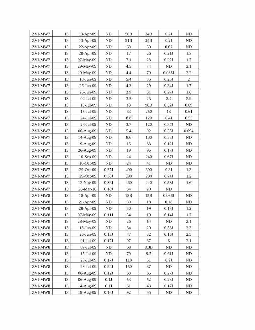
ZVI-MW7 13 13-Apr-09 ND 50B 24B 0.2J ND
ZVI-MW7 13 13-Apr-09 ND 51B 24B 0.2J ND
ZVI-MW7 13 22-Apr-09 ND 68 50 0.67 ND
ZVI-MW7 13 28-Apr-09 ND 17 26 0.21J 1.3
ZVI-MW7 13 07-May-09 ND 7.1 28 0.22J 1.7
ZVI-MW7 13 29-May-09 ND 4.5 74 ND 2.1
ZVI-MW7 13 29-May-09 ND 4.4 70 0.085J 2.2
ZVI-MW7 13 18-Jun-09 ND 5.4 35 0.25J 2
ZVI-MW7 13 26-Jun-09 ND 4.3 29 0.34J 1.7
ZVI-MW7 13 26-Jun-09 ND 3.9 31 0.27J 1.8
ZVI-MW7 13 02-Jul-09 ND 3.5 25 3.4 2.9
ZVI-MW7 13 10-Jul-09 ND 13 90B 0.32J 0.69
ZVI-MW7 13 15-Jul-09 ND 63 250 13 0.61
ZVI-MW7 13 24-Jul-09 ND 8.8 120 0.4J 0.53
ZVI-MW7 13 28-Jul-09 ND 3.7 120 0.37J ND
ZVI-MW7 13 06-Aug-09 ND 5.4 92 0.36J 0.094
ZVI-MW7 13 14-Aug-09 ND 8.6 150 0.53J ND
ZVI-MW7 13 19-Aug-09 ND 15 83 0.12J ND
ZVI-MW7 13 26-Aug-09 ND 19 95 0.17J ND
ZVI-MW7 13 10-Sep-09 ND 24 240 0.67J ND
ZVI-MW7 13 16-Oct-09 ND 24 41 ND ND
ZVI-MW7 13 29-Oct-09 0.37J 400 300 0.8J 1.3
ZVI-MW7 13 29-Oct-09 0.36J 390 280 0.74J 1.2
ZVI-MW7 13 12-Nov-09 0.39J 460 240 0.53J 1.6
ZVI-MW7 13 26-Mar-10 0.18J 34 20 ND
ZVI-MW8 13 10-Apr-09 ND 18B 15B 0.066J ND
ZVI-MW8 13 21-Apr-09 ND 39 18 0.18 ND
ZVI-MW8 13 28-Apr-09 ND 30 19 0.13J 1.2
ZVI-MW8 13 07-May-09 0.11J 54 19 0.14J 1.7
ZVI-MW8 13 28-May-09 ND 26 14 ND 2.1
ZVI-MW8 13 18-Jun-09 ND 34 20 0.53J 2.3
ZVI-MW8 13 26-Jun-09 0.15J 77 32 0.15J 2.5
ZVI-MW8 13 01-Jul-09 0.17J 97 37 6 2.1
ZVI-MW8 13 09-Jul-09 ND 68 8.3B ND ND
ZVI-MW8 13 15-Jul-09 ND 79 9.5 0.61J ND
ZVI-MW8 13 23-Jul-09 0.17J 110 51 0.2J ND
ZVI-MW8 13 28-Jul-09 0.22J 150 37 ND ND
ZVI-MW8 13 06-Aug-09 0.12J 63 66 0.27J ND
ZVI-MW8 13 06-Aug-09 0.1J 53 52 0.23J ND
ZVI-MW8 13 14-Aug-09 0.1J 61 43 0.17J ND
ZVI-MW8 13 19-Aug-09 0.16J 92 35 ND ND

ZVI-MW8 13 26-Aug-09 0.6J 83 33 ND ND
ZVI-MW8 13 10-Sep-09 0.16J 110 21 0.11J ND
ZVI-MW8 13 16-Oct-09 0.095J 89 11 ND ND
ZVI-MW8 13 29-Oct-09 ND 79 96 ND 0.42
ZVI-MW8 13 12-Nov-09 0.7J 770 67 0.42J ND
ZVI-MW8 13 25-Mar-10 0.69J 400 87 ND ND
ZVI-MW9 13 13-Apr-09 0.087J 49B 10B 0.54J ND
ZVI-MW9 13 22-Apr-09 0.21 57 15 0.57 0.13
ZVI-MW9 13 28-Apr-09 ND 41 12 0.39J ND
ZVI-MW9 13 07-May-09 0.13J 50 9.5 0.54J ND
ZVI-MW9 13 28-May-09 ND 31 9.7 ND ND
ZVI-MW9 13 18-Jun-09 ND 19 7.6 .28J ND
ZVI-MW9 13 26-Jun-09 ND 26 8.3 0.18J ND
ZVI-MW9 13 02-Jul-09 ND 27 8.4 1.5 ND
ZVI-MW9 13 10-Jul-09 ND 94 13B 0.61J ND
ZVI-MW9 13 15-Jul-09 0.12J 89 10 0.79J ND
ZVI-MW9 13 24-Jul-09 0.16JB 79 21 0.64J 1
ZVI-MW9 13 28-Jul-09 ND 23 60 0.61J 0.39J
ZVI-MW9 13 07-Aug-09 ND 24 77 0.9J 6.6
ZVI-MW9 13 14-Aug-09 ND 13 130 1.7 16
ZVI-MW9 13 20-Aug-09 ND 16 140 1.7 17
ZVI-MW9 13 27-Aug-09 ND 14 380 4.2 30
ZVI-MW9 13 10-Sep-09 ND 19 520 5.4 28
ZVI-MW9 13 15-Oct-09 0.23J 34 360B 4.6 18
ZVI-MW9 13 29-Oct-09 ND 45 390 4.3 11
ZVI-MW9 13 12-Nov-09 ND 60 200 2.8 8.9
ZVI-MW9 13 25-Mar-10 0.21J 37 7.9 0.15J ND