combining pixel swapping and contouring methods to enhance super-resolution mapping

1428 IEEE JOURNAL OF SELECTED TOPICS IN APPLIED EARTH OBSERVATIONS AND REMOTE SENSING, VOL. 5, NO. 5, OCTOBER 2012

Combining Pixel Swapping and Contouring Methodsto Enhance Super-Resolution Mapping

Yuan-Fong Su, Giles M. Foody, Senior Member, IEEE, Anuar M. Muad, and Ke-Sheng Cheng

Abstract—Combining super-resolution techniques can increasethe accuracy with which the shape of objects may be characterisedfrom imagery. This is illustrated with two approaches to combiningthe contouring and pixel swapping methods of super-resolutionmapping for binary classification applications. In both approaches,the output of the pixel swapping method is softened to allow a con-tour of equal class membership to be fitted to it to represent theinter-class boundary. The accuracy of super-resolution mappingwith the individual and combined techniques is explored, includingan assessment of the effect of variation in the number of neighborsand zoom factor on pixel swapping based analyses. When com-bined, the error with which objects of varying shape were repre-sented was typically greatly reduced relative to that observed fromthe application of the methods individually. For example, the rootmean square error inmapping the boundary of an aeroplane repre-sented in relatively fine spatial resolution imagery decreased from14.41 m with contouring and 4.35 m with pixel swapping to 3.07 mwhen the approaches were combined.

Index Terms—Contour-based approach, pixel swapping, softclassification, super-resolution mapping.

I. INTRODUCTION

T HEmixed pixel problem is a common challenge in patternrecognition applications based on remotely sensed data.

Many popular analyses, such as land cover mapping via con-ventional classification, assume pixels to be pure but remotelysensed imagery may contain a large proportion of mixed pixels[1], [2]. The mixed pixel problem is commonly noted in relationto analyses of coarse spatial resolution imagery. However, themixed pixel problem is not constrained to coarse resolution im-agery, it may, for example, arise at fine spatial resolutions as aninteractive function of target size relative to the pixel size as well

Manuscript received April 28, 2012; revised July 08, 2012; accepted August20, 2012. Date of publication October 19, 2012; date of current versionNovember 14, 2012. This work was supported in part by National ScienceCouncil, Taiwan NSC98-2917-I-564-118 for YFS and supported in part byUniversiti Kebangsaan Malaysia, Malaysia for AMM.Y. F. Su was with the Department of Bioenvironmental Systems Engineering,

National Taiwan University, Taiwan. He is now with the National Science andTechnology Center for Disaster Reduction, New Taipei City 231, Taiwan (cor-responding author, e-mail: [email protected]; [email protected]).G. M. Foody is with the School of Geography, University of Nottingham,

University Park, Nottingham, NG7 2RD U.K. (e-mail: [email protected]).A. M. Muad was with the School of Geography, University of Not-

tingham, University Park, Nottingham, NG7 2RD U.K. He is now with theDepartment of Electrical, Electronic and Systems Engineering, UniversitiKebangsaan Malaysia, 43600 UKM Bangi, Selangor, Malaysia (e-mail:[email protected]).K. S. Cheng is with the Department of Bioenvironmental Systems En-

gineering, National Taiwan University, Taipei, Taiwan 10617 (e-mail:[email protected]).Digital Object Identifier 10.1109/JSTARS.2012.2216514

as through an increase in intra-class variation [3], [4]. Consid-erable research has been directed to addressing the mixed pixelproblem for applications such as land cover mapping. In partic-ular, the use of fuzzy or soft image classifications that allow apixel to have multiple and partial class memberships in order toaccommodate the effects of mixed pixels has become common-place [5]–[7]. However, information on the spatial distributionof the classes within a pixel is not specified by a soft classi-fication but is often desired [8]–[11]. For example, the spatialconfiguration of the landscape mosaic is fundamental to studiesof landscape ecology or to users of spatially explicit models.Super-resolution mapping is one means to reduce the mixed

pixel problem. Guided by the class composition informationprovided by a soft classification, a super-resolution mappinganalysis seeks to locate the land covers geographically at a sub-pixel scale. A variety of super-resolution mapping techniqueshas been used in remote sensing [12]–[20]. A key feature withthese techniques is an assumption of spatial continuity, with lo-cations near to each other more alike than those that are furtherapart [13], [20]. The methods, however, vary greatly. One com-putationally simple approach for a binary classification scenariousing a soft classification output that represents the class com-position in terms of proportional cover is to fit an isoline of equalclass membership, the 0.5 class membership contour, to the softclassification to represent the boundary between the componentclasses [14]. Although simple and effective this method has lim-itations, notably in relation to failing to maintain the class com-position information, especially where the boundary may bendsharply. An alternative but more demanding analysis is to uti-lize an approach such as pixel swapping (PS; [13], [21]–[23])or a Hopfield neural network (HNN; [20]) that seeks to main-tain the class composition information of the soft classification.These algorithms are, however, not without problems. Thereare concerns, for example, that as the PS slavishly maintainsthe class composition information conveyed by the soft clas-sification it is highly sensitive to the accuracy of that classi-fication. With the HNN, one of the major concerns is that ittends to produce rounded corners and, therefore, may some-times poorly represent land cover patches with complex shape,especially if the patch boundary has sharp corners [24]. Withboth the PS and HNN, the boundary between classes is also stillconstrained to lie between pure units, here sub-pixels, giving anunrealistic serrated representation. Additionally, there are con-cerns that the predicted location of land covers within the areaof a pixel may be imperfect, especially if there are small landcover patches [25].A contour-based super-resolution mapping technique, the

contour-based Hopfield neural network (CHNN), was recently

1939-1404/$31.00 © 2012 IEEE

SU et al.: COMBINING PIXEL SWAPPING AND CONTOURING METHODS TO ENHANCE SUPER-RESOLUTION MAPPING 1429

proposed [20]. The latter combines the contouring and HNNtwo super-resolution approaches, yielding outputs that are moreaccurate than each alone. However, a limitation of the CHNN isthat it inherits the aforementioned concerns of the HNN. If thesoft classification is accurate, PS may be more suitable than theHNN for super-resolution mapping. Thus, combining the con-touring and PS based approaches may be one way to enhancesuper-resolution analysis. The contour-based PS (CPS) methodseeks to exploit the positive features of the contouring and PSsuper-resolution mapping approaches to produce a method thatis more accurate than each alone. Although the standard PSalgorithm has been used for multi-class applications [26], [27],this is illustrated with a binary classification scenario used inmany other studies [13], [15], [20], [21].The remainder of this paper is organized as follows. In

Section 2, contour-based super-resolution mapping techniquesare introduced. Section 3 introduces the simulated and satelliteimagery as well as methods used to explore the potential of theCPS approach and selected comparator methods (contouring,PS and CHNN). In Section 4, results of super-resolutionmapping provided by PS, contouring, CHNN and CPS werecompared. Finally, Section 5 provides a summary and conclu-sion of the findings with particular regard to the CPS approachto super-resolution mapping.

II. CONTOUR-BASED SUPER-RESOLUTION MAPPING

The contouring approach to super-resolution mapping in-volves fitting of a 0.5 class membership contour to the softclassification that indicates the proportional cover of the twoclasses to be represented. The contour fitted to the output of asoft classification provides a representation of the boundary ofland cover patches. Here, a 0.5 class membership contour wasused to separate two classes: a target object and its background.This approach allows the contour to run through pixels and canprovide smooth boundaries rather than unrealistic jagged onesthat arise when boundaries are fitted to hard classifications andconstrained to lie between pixels.With the PS method of super-resolution mapping, each pixel

is sub-divided into a set of typically equal sized sub-pixels. Therelative increase in spatial resolution from pixel-level to sub-pixel-level is referred to as the zoom factor . The class com-position information conveyed by the soft classification is usedto determine the number of sub-pixels allocated to each class.The analysis begins with the allocated proportion of sub-pixelslabeled to each class distributed randomlywithin the pixel’s areaand proceeds until an optimal spatial configuration of labeledsub-pixels is produced. The analysis itself is based upon the at-tractiveness of each sub-pixel for a particular class. A variety ofapproaches to varying the spatial arrangement of the sub-pixelclass labels exist but the basic approach adopted here has threesteps. First, the attractiveness of a sub-pixel is predicted asa distance-weighted function of its neighboringsub-pixels:

(1)

where is the binary class (0 or 1) of the th sub-pixel atlocation , and is a distance-dependent weight function ofthe form:

(2)

where is the distance between the sub-pixel for which theattractiveness is to be computed and a neighboring sub-pixel ,and is the non-linear parameter of the exponential model [13].In the second step, once the attractiveness of each sub-pixel

location has been estimated on the basis of the current arrange-ment of sub-pixel class labels, the algorithm ranks the scores ona pixel-by-pixel basis. For each pixel, the least attractive loca-tion at which the sub-pixel is currently allocated to “1” (e.g., a“1” surrounded mainly by “0”s) is selected as candidate A:

(3)

Similarly, the most attractive location at which the sub-pixel iscurrently allocated to a “0” (e.g., a “0” surrounded mainly by“1”s) is also selected as candidate B:

(4)

In the third step, sub-pixel class labels may be swapped, be-tween candidates A and B, to achieve a more suitable spatialconfiguration of the sub-pixel class labels. Specifically, if the at-tractiveness of the least attractive location (candidate A) is lessthan that of the most attractive location (candidate B), then theclass labels for that pair of sub-pixels are swapped:

(5)

Note that in the standard PS method the swapping of class labelsis constrained such that it occurs within pixels only, and hencethe class compositional information of the soft classification ismaintained throughout the analysis. The three steps are repeateduntil no swaps are made or when a pre-specified number of iter-ations has been completed. The boundary between classes maythen be fitted between sub-pixels that differ in label. Althoughthis allows a boundary to be located at a sub-pixel scale theboundary may still have an unrealistic jagged edge as it is stillconstrained to lie between units, sub-pixels, allocated differentclasses.Several parameters need to be set by the investigator when

using the PS method. Two key parameters are the number ofneighboring sub-pixels and the non-linear parameter of theexponential function. The number of neighboring sub-pixels hastypically been set to a low value, often in the range 1–5 [13];when the number is 1 this means that the analysis is based uponthe eight immediate sub-pixel neighbors that lie within a 3 3window centred on the sub-pixel of interest.The key feature of the proposed CPS approach is the fitting

of a 0.5 class membership contour to the result of a PS-basedanalysis. To achieve this, the output of the PS analysis mustbe softened from the conventional scenario in which sub-pixelsare allocated a single class label (i.e., hard classified). Here, twoapproaches to softening the output of the conventional PS basedapproach were evaluated. The first, denoted by CPS1 hereafter,


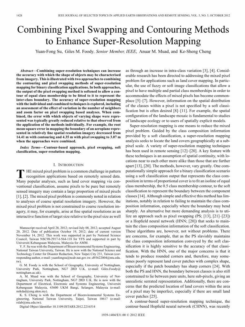
Fig. 1. Basis of the PS, CPS1, and CPS2 methods. Upper left image is a 2 2pixels image with randomly located sub-pixels and the zoom factor is 5. Lowerleft image is the result of standard PS. The images on the right are the softenedproportion image produced from CPS1 and CPS2.

is based on the normalized attractiveness as a prediction ofclass proportion at a sub-pixel scale. For this, (1) is normalizedto the range of 0 to 1:

(6)

in which the denominator is the summation of the distance-de-pendent weights calculated from the user-defined neighboringsub-pixels. A 0.5 class membership contour may then be fittedto the normalized attractiveness to represent the inter-classboundary. With the CPS1 method, the attractiveness is dividedby the summation of the distance-dependent weight function.Thus, (6) could be regarded as the sub-pixel class label passingthrough a smoothing filter with the window size defined by thenumber of neighboring sub-pixels. Therefore, it is expected thatthe class proportion information used will vary with the selectednumber of neighboring sub-pixels and the non-linear parametervalue used. Note that as the window size gets bigger not onlythe output of CPS1 becomes smoother but also increases thepotential for effects from other, not neighboring, class patches.In the second approach, denoted by CPS2 hereafter, the

output of the conventional PS method is softened in a differentway. A prediction of the proportion class cover for a sub-pixel isderived from the average of the labels (0, 1) for its surrounding8 sub-pixels:

(7)

By using only the surrounding 8 sub-pixels the danger that thepredicted class proportion was negatively affected by the pres-ence of other, but separate, class patches is reduced. Thus, theCPS2 adds one additional step to the standard PS method andproduces a predicted proportional image. As with CPS1, the lo-cation of the inter-class boundary may then be represented asthe 0.5 class membership contour fitted to the predicted classproportional cover image.A summary of the CPS1 and CPS2 methods is given in Fig. 1.

There are twomajor differences between the twomethods. First,

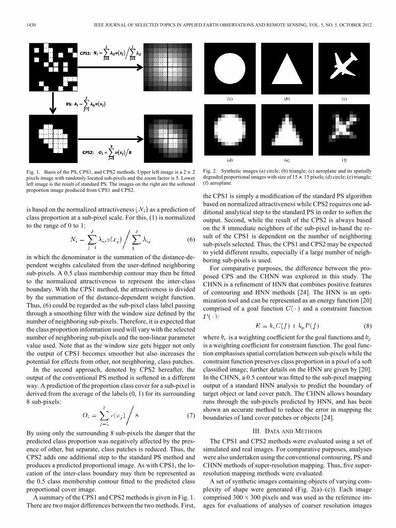
Fig. 2. Synthetic images (a) circle; (b) triangle; (c) aeroplane and its spatiallydegraded proportional images with size of 15 15 pixels; (d) circle; (e) triangle;(f) aeroplane.

the CPS1 is simply a modification of the standard PS algorithmbased on normalized attractiveness while CPS2 requires one ad-ditional analytical step to the standard PS in order to soften theoutput. Second, while the result of the CPS2 is always basedon the 8 immediate neighbors of the sub-pixel in-hand the re-sult of the CPS1 is dependent on the number of neighboringsub-pixels selected. Thus, the CPS1 and CPS2 may be expectedto yield different results, especially if a large number of neigh-boring sub-pixels is used.For comparative purposes, the difference between the pro-

posed CPS and the CHNN was explored in this study. TheCHNN is a refinement of HNN that combines positive featuresof contouring and HNN methods [24]. The HNN is an opti-mization tool and can be represented as an energy function [20]comprised of a goal function and a constraint function

(8)

where is a weighting coefficient for the goal functions andis a weighting coefficient for constraint function. The goal func-tion emphasises spatial correlation between sub-pixels while theconstraint function preserves class proportion in a pixel of a softclassified image; further details on the HNN are given by [20].In the CHNN, a 0.5 contour was fitted to the sub-pixel mappingoutput of a standard HNN analysis to predict the boundary oftarget object or land cover patch. The CHNN allows boundaryruns through the sub-pixels predicted by HNN, and has beenshown an accurate method to reduce the error in mapping theboundaries of land cover patches or objects [24].

III. DATA AND METHODS

The CPS1 and CPS2 methods were evaluated using a set ofsimulated and real images. For comparative purposes, analyseswere also undertaken using the conventional contouring, PS andCHNN methods of super-resolution mapping. Thus, five super-resolution mapping methods were evaluated.A set of synthetic images containing objects of varying com-

plexity of shape were generated (Fig. 2(a)–(c)). Each imagecomprised 300 300 pixels and was used as the reference im-ages for evaluations of analyses of coarser resolution images


Fig. 3. The Formosat-II panchromatic images (a) a high reflectance roof offactory with size of 150 150 pixels; (b) the hard classification of the objectextracted from (a) and its degraded proportional images (c) with size of 15 15pixels and (d) with size of 10 10 pixels; (e) two factory roof with size of180 360 pixels; (f) the classified object extracted from (e) and its degradedproportional images (g) with size of 18 36 pixels and (h) with size of 12 24pixels; (i) another set of simulated satellite images degraded from (a) with size of15 15 pixels and (j) with size of 10 10 pixels; (k) soft classification derivedfrom (i); (l) soft classification from (j); (m) simulated satellite images degradedfrom (e) with size of 18 36 pixels and (n) with size of 12 24 pixels; (o) softclassification derived from (m); (p) soft classification from (n).

derived from them. The reference images were binary to sim-ulate the hard classification comprising two classes (0, 1). Thefine-resolution synthetic images were degraded spatially by theuse of an average filter to form coarser resolution synthetic pro-portional images with size of 15 15 pixels (Fig. 2(d)–(f)). Thefive super-resolutionmappingmethods were applied to the latterimages and their outputs evaluated against the representationdepicted in the relevant reference image.In addition to the synthetic data sets, a series of analyses were

undertaken using real satellite sensor imagery. Specifically,attention focused on clearly defined objects in a Formosat-IIPanchromatic image of Northern Taiwan acquired on 29 July2006 with spatial resolution of 2 m. Here, attention focusedon the factory roofs of differing shape, size and orientation(Fig. 3(a) with size of 150 150 pixels and Fig. 3(e) with sizeof 180 360 pixels). Again, the fine spatial resolution imagewas used as reference data for analyses undertaken on spatiallydegraded versions of the data. With the Formosat-II image data,analyses were undertaken with the data degraded by a factorof 10 (i.e., to 20 m resolution) and 15 (i.e., to 30 m resolution)to equate roughly to imagery from popular remote sensingsystems such as SPOT HRV and Landsat . Coarseresolution imagery were, however, derived in two ways. First,the proportional images derived from the application of a hardclassification to the original image with a spatial resolution of2 m were degraded spatially. This was achieved by aggregating

Fig. 4. Impact of and on PS-based analysis for a block of 4 4 pixels zoomfactor of 5. The number of neighboring sub-pixels for left figure diagram is 3(yielding a neighboring ratio of ) while for right diagram it is 6(yielding a neighboring ratio of ). Note that the sub-pixels in lightergray are those used for calculation of attractiveness and assign the attractivenessto the dark gray sub-pixel . In right diagram, the attractiveness of the sub-pixelwhich belongs to the pixel l highlighted by bold solid grid is affected by blacksub-pixel which is belong to another pixel (highlighted by bold dash grid) thatis not an immediate neighbor.

pixels to yield a set of simulated images with spatial resolutionsof 20 m and 30 m (Fig. 3(c)–(d) and (g)–(h)). This approachensured that the class proportional composition informationover all regions was maintained at all resolutions evaluated. Togain a more realistic simulation of coarse resolution imagery asecond set of simulated coarse resolution images were derived.This was achieved by degrading spatially the 2 m spatial reso-lution images (Fig. 3(a) and (e)) to 20 m (Fig. 3(i), (m)) and 30m (Fig. 3(j), (n)) resolution by an average filter and applying asoft classification to those data.The soft classifications upon which the super-resolution

analyses were based were derived using the fuzzy -means(FCM) algorithm [28]. Additionally, hardened versions of thesoft classification of the original, fine spatial resolution, imageswere used as reference data in the determination of the accuracyof the super-resolution mapping. In all cases the weightingcomponent in the fuzzy -means classifications, whichdetermines the degree of fuzziness, was set to 2.0.The closeness of the predicted boundary to the actual

boundary in the relevant reference image was indicated bythe root mean square error (RMSE) and mean absolute error(MAE) calculated on the distances measured between the pre-dicted and reference boundaries. To aid comparability betweenthe five super-resolution mapping techniques used, the distancefrom the same set of points along the reference boundary wereused in all comparisons. The latter were defined with the aid ofthe output from the standard PS. Specifically, the shortest dis-tance between the boundary predicted by the standard PS andreference was calculated at every sub-pixel along the predictedboundary. The point on the reference boundary used in thisassessment was then used in the evaluation of the accuracy ofthe predictions from the other four methods: contouring, CPS1,CPS2 and CHNN.The number of neighboring sub-pixels, , is a critical param-

eter in standard PS algorithm and the two CPS methods. How-ever, there is little advice in the literature on the determination


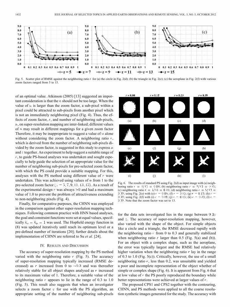
Fig. 5. Scatter plot of RMSE against the neighboring ratio for (a) the circle in Fig. 2(d); (b) the triangle in Fig. 2(e); (c) the aeroplane in Fig. 2(f) with variouszoom factors ranged from 5 to 15.

of an optimal value. Atkinson (2005) [13] suggested an impor-tant consideration is that the should not be too large. When thevalue of is larger than the zoom factor, a sub-pixel within apixel could be attracted to sub-pixels from another pixel whichis not an immediately neighboring pixel (Fig. 4). Thus, the ef-fects of zoom factor, , and number of neighboring sub-pixels,, on super-resolutionmapping are inter-linked; different valuesof may result in different mappings for a given zoom factorTherefore, it may be inappropriate to suggest a value of alonewithout considering the zoom factor. A neighboring ratio ,which is derived from the number of neighboring sub-pixels di-vided by the zoom factor, is suggested in this study to expressand together. An experiment to help suggest a suitable range of, to guide PS-based analyses was undertaken and sought espe-cially to help guide the selection of an appropriate value for thenumber of neighboring sub-pixels for pre-selected zoom factor,with which the PS could provide a suitable mapping. For this,analyses with the PS method using different value of wereundertaken. This was achieved using values of from 1 to thepre-selected zoom factor . As a result ofthe experimental design was always and had a maximumvalue of 1.0 to prevent the problem of attractiveness extendingto non-neighboring pixels (Fig. 4).Finally, for comparative purposes, the CHNN was employed

in the comparison against other super-resolution mapping tech-niques. Following common practice with HNN based analyses,the goal and constraint functions were set at equal values, specif-ically was used. The Hopfield energy function in(8) was updated iteratively until reach its optimum level or apre-defined number of iterations [20]; further details about theimplementation of CHNN are referred to Su et al. [24].

IV. RESULTS AND DISCUSSION

The accuracy of super-resolution mapping by the PS methodvaried with the neighboring ratio (Fig. 5). The accuracyof super-resolution mapping typically increased (RMSE de-creased) as increased from 0 to and was thereafterrelatively stable for all object shapes analysed as increasedto its maximum value of 1. Therefore, a suitable value of theneighboring ratio appears to lie in the range of 0.3 to 1.0(Fig. 5). This result also suggests that when an investigatorselects a zoom factor for use with the PS algorithm, anappropriate setting of the number of neighboring sub-pixels

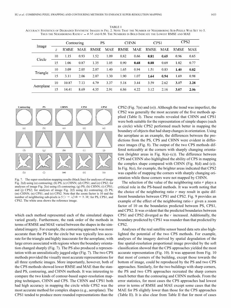
Fig. 6. The results of standard PS using Fig. 2(d) as input image with (a) neigh-boring ratio ; (b) neighboring ratio ;(c) neighboring ratio ; (d) neighboring ratio

; using Fig. 2(e) with (e) ; (f) ; (g) ; (h); using Fig. 2(f) with (i) ; (j) ; (k) ; (l). Note that the zoom factor was set to 13.

for the data sets investigated lies in the range betweenand . The accuracy of super-resolution mapping, however,also varied with the shape of the object. For simple objectslike a circle and a triangle, the RMSE decreased rapidly withthe neighboring ratio from 0 to 0.3 and generally stabilizedwhen neighboring ratio larger than 0.5 (Fig. 5(a) and (b)).For an object with a complex shape, such as the aeroplane,the error was typically largest and the RMSE had relativelyhigher variation when the neighboring ratio lay in the rangeof 0.3 to 1.0 (Fig. 5(c)). Critically, however, the use of a smallneighboring ratio , less than 0.2, was unsuitable and yieldeda poor and incomplete representation of the object whether ofsimple or complex shape (Fig. 6). It is apparent from Fig. 6 thatat low value of the PS poorly reproduced the boundary whilebetter representations were achieved at larger values of .The proposed CPS1 and CPS2 together with the contouring,

CHNN, and PS methods were applied to all the coarse resolu-tion synthetic images generated for the study. The accuracy with


TABLE IACCURACY STATISTICS OF DEGRADED SYNTHETIC IMAGES IN FIG. 2. NOTE THAT THE NUMBER OF NEIGHBORING SUB-PIXELS WAS SET TO 5.

THUS THE NEIGHBORING RATIO AND 0.50. THE NUMBERS IN BOLD INDICATE THE LOWEST RMSE AND MAE

Fig. 7. The super-resolution mapping results (black line) for analyses of imageFig. 2(d) using (a) contouring; (b) PS; (c) CHNN; (d) CPS1; and (e) CPS2; foranalyses of image Fig. 2(e) using (f) contouring; (g) PS; (h) CHNN; (i) CPS1;and (j) CPS2; for analyses of image Fig. 2(f) using (k) contouring; (l) PS;(m) CHNN; (n) CPS1; and (o) CPS2. Note that the zoom factor is 10 and thenumber of neighboring sub-pixels is 5 for PS, CPS1, andCPS2. The white area shows the reference image.

which each method represented each of the simulated shapesvaried greatly. Furthermore, the rank order of the methods interms of RMSE and MAE varied between the shapes in the sim-ulated imagery. For example, the contouring approachwasmoreaccurate than the PS for the circle but was typically less accu-rate for the triangle and highly inaccurate for the aeroplane, withlarge errors associated with regions where the boundary orienta-tion changed sharply (Fig. 7). The PS also produced a represen-tation with an unrealistically jagged edge (Fig. 7). The two CPSmethods provided the visually most accurate representations forall three synthetic images. More importantly, however, both ofthe CPS methods showed lower RMSE and MAE than the stan-dard PS, contouring, and CHNN methods. It was interesting tocompare the two kinds of contour-based super-resolution map-ping techniques, CHNN and CPS. The CHNN and CPS1 bothhad high accuracy in mapping the circle while CPS2 was themost accurate method for complex shapes (e.g., aeroplane). TheCPS1 tended to produce more rounded representations than the

CPS2 (Fig. 7(n) and (o)). Although the trend was imperfect, theCPS2 was generally the most accurate of the five methods ap-plied (Table I). These results revealed that CHNN and CPS1were both suitable for the representation of simple shapes (suchas circle) while CPS2 performed much better in mapping theboundary of objects that had sharp changes in orientation. Usingthe aeroplane as an example, the differences between the pre-dictions from the PS, CPS and CHNN were evident in differ-ence images (Fig. 8). The output of the two CPS methods dif-fered noticeably at the corners with sharply changing orienta-tion (brighter areas in Fig. 8(a)–(c)). The difference betweenCPS and CHNN also highlighted the ability of CPS in mappingthe complex shape compared with CHNN (Fig. 8(d) and (e)).In Fig. 8(e), for example, the brighter areas indicated that CPS2was capable of mapping the corners with sharply changing ori-entation while those corners were not mapped by CHNN.The selection of the value of the neighboring ratio plays a

critical role in the PS-based methods. It was worth noting thatthe choice of the neighboring ratio may result in quite dif-ferent boundaries between CPS1 and CPS2. Fig. 9 provides anexample of the effect of the neighboring ratio given a zoomfactor of 10 on the boundaries predicted between PS, CPS1,and CPS2. It was evident that the predicted boundaries betweenCPS1 and CPS2 diverged as the increased. Additionally, theboundary predicted by CPS1 was rounder than that predicted byCPS2.Analyses of the real satellite sensor based data sets also high-

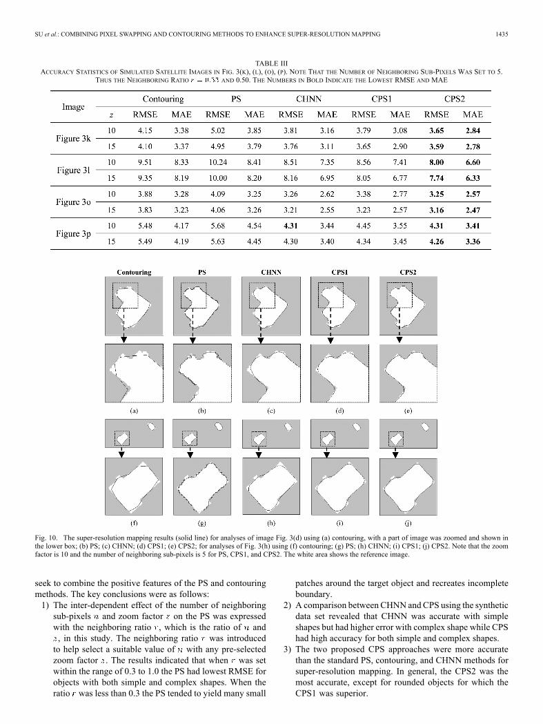
lighted the potential of the two CPS methods. For example,analyses of the imagery derived by spatial degradation of thefine spatial-resolution proportional image provided by the softclassification showed that the CPS approaches yielded the mostaccurate representation (Fig. 10). It was apparent from Fig. 10that most of corners of the building, except those towards thebottom of image, could be reproduced by the PS and two CPSapproaches. Similarly, for the two buildings with sharp corners,the PS and two CPS approaches recreated the sharp cornersmuch better than the contouring and CHNN methods. From theerror statistics, for most cases the CPS approaches had lowesterror in terms of RMSE and MAE except some cases that theMAE for PS slightly lower than those for the CPS approaches(Table II). It is also clear from Table II that for most of cases


Fig. 8. The difference images of super-resolution mapping results derived from various methods. (a) CPS1-PS; (b) CPS2-PS; (c) CPS2-CPS1; (d) CPS1-CHNN;(e) CPS2-CHNN. The black line shows the reference boundary.

TABLE IIACCURACY STATISTICS OF SIMULATED SATELLITE IMAGES IN FIG. 3(C), (D), (G), (H). NOTE THAT THE NUMBER OF NEIGHBORING SUB-PIXELS WAS SET TO 5.


Fig. 9. Illustration of the difference between PS, CPS1 and CPS2 with variousratio of (a) ; (b) ; (c) using the sharpcorner on top of Fig. 2(e) as an example. Note that the zoom factor was set to10.

with a zoom factor of 15 had lower error than that with a zoomfactor of 10.Different trends were observed for the second set of simu-

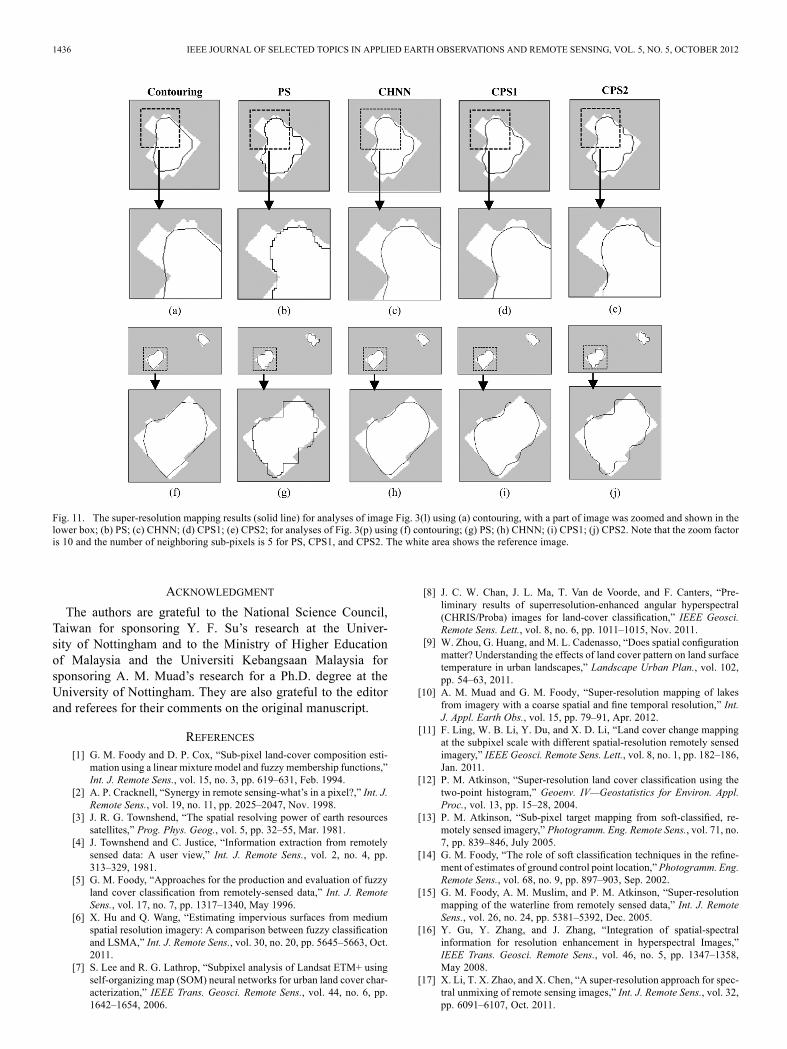
lated satellite images. Here, the PS and two CPS methods re-produced distorted boundaries (Fig. 11). This result occurredbecause the proportional information in this set of images wasnot maintained across all resolutions but varied between the im-ages with the spatial resolution of 20 m and 30 m. This problemis linked to the quality of the soft classification upon which thesuper-resolution mapping is based [29]. It may be possible toincrease the quality of the soft classification and thereby super-resolution mapping by, for example, adding ancillary informa-tion [30], [31]. However, the CPS1 and CPS2 still had better per-formance, in terms of RMSE andMAE, than the PS, contouring,and CHNN methods (Table III) perhaps highlighting the effect

of variation in soft classification accuracy on the accuracy ofsuper-resolution mapping. Interestingly, the contouring methodwas more accurate than the PS, the opposite of the results de-rived from the other set of simulated satellite images (Table III).Critically, however, the two CPS approaches were again sub-stantially more accurate than the standard PS, contouring, andCHNNmethods in terms of both the measured RMSE andMAE(Tables II and III). Typically, to help put the results into context,for simple and complex objects (Table I) the RMSEs observedfrom the CPS2 were smaller than those associated with the con-touring and PS by a factor of to and to

, respectively. For example, the biggest difference wasfor the aeroplane (Fig. 2(f)) for which the RMSE was 14.41 min contouring, 4.35 m in PS and 3.07 m in the CPS2; while theMAE was 8.69 m in contouring, 2.91 m in PS and 2.06 m in theCPS2.

V. CONCLUSION

Super-resolution mapping provides a means to represent ob-jects at a sub-pixel scale from the class proportional image pro-vided by a soft classification. In approaches such as the PS, thepredicted boundary is jagged because its location must lie be-tween sub-pixels. While the contouring method may be able tobreak limit of pixel grid it can mis-represent the shape and areaof an object. Combining the PS and contouring approaches maybe one way to enhance super-resolution mapping. This studyproposed two contour-based pixel swapping approaches that


TABLE IIIACCURACY STATISTICS OF SIMULATED SATELLITE IMAGES IN FIG. 3(K), (L), (O), (P). NOTE THAT THE NUMBER OF NEIGHBORING SUB-PIXELS WAS SET TO 5.


Fig. 10. The super-resolution mapping results (solid line) for analyses of image Fig. 3(d) using (a) contouring, with a part of image was zoomed and shown inthe lower box; (b) PS; (c) CHNN; (d) CPS1; (e) CPS2; for analyses of Fig. 3(h) using (f) contouring; (g) PS; (h) CHNN; (i) CPS1; (j) CPS2. Note that the zoomfactor is 10 and the number of neighboring sub-pixels is 5 for PS, CPS1, and CPS2. The white area shows the reference image.

seek to combine the positive features of the PS and contouringmethods. The key conclusions were as follows:1) The inter-dependent effect of the number of neighboringsub-pixels and zoom factor on the PS was expressedwith the neighboring ratio , which is the ratio of and, in this study. The neighboring ratio was introducedto help select a suitable value of with any pre-selectedzoom factor . The results indicated that when was setwithin the range of 0.3 to 1.0 the PS had lowest RMSE forobjects with both simple and complex shapes. When theratio was less than 0.3 the PS tended to yield many small

patches around the target object and recreates incompleteboundary.

2) A comparison between CHNN and CPS using the syntheticdata set revealed that CHNN was accurate with simpleshapes but had higher error with complex shape while CPShad high accuracy for both simple and complex shapes.

3) The two proposed CPS approaches were more accuratethan the standard PS, contouring, and CHNN methods forsuper-resolution mapping. In general, the CPS2 was themost accurate, except for rounded objects for which theCPS1 was superior.


Fig. 11. The super-resolution mapping results (solid line) for analyses of image Fig. 3(l) using (a) contouring, with a part of image was zoomed and shown in thelower box; (b) PS; (c) CHNN; (d) CPS1; (e) CPS2; for analyses of Fig. 3(p) using (f) contouring; (g) PS; (h) CHNN; (i) CPS1; (j) CPS2. Note that the zoom factoris 10 and the number of neighboring sub-pixels is 5 for PS, CPS1, and CPS2. The white area shows the reference image.

ACKNOWLEDGMENT

The authors are grateful to the National Science Council,Taiwan for sponsoring Y. F. Su’s research at the Univer-sity of Nottingham and to the Ministry of Higher Educationof Malaysia and the Universiti Kebangsaan Malaysia forsponsoring A. M. Muad’s research for a Ph.D. degree at theUniversity of Nottingham. They are also grateful to the editorand referees for their comments on the original manuscript.

REFERENCES[1] G. M. Foody and D. P. Cox, “Sub-pixel land-cover composition esti-

mation using a linear mixture model and fuzzy membership functions,”Int. J. Remote Sens., vol. 15, no. 3, pp. 619–631, Feb. 1994.

[2] A. P. Cracknell, “Synergy in remote sensing-what’s in a pixel?,” Int. J.Remote Sens., vol. 19, no. 11, pp. 2025–2047, Nov. 1998.

[3] J. R. G. Townshend, “The spatial resolving power of earth resourcessatellites,” Prog. Phys. Geog., vol. 5, pp. 32–55, Mar. 1981.

[4] J. Townshend and C. Justice, “Information extraction from remotelysensed data: A user view,” Int. J. Remote Sens., vol. 2, no. 4, pp.313–329, 1981.

[5] G. M. Foody, “Approaches for the production and evaluation of fuzzyland cover classification from remotely-sensed data,” Int. J. RemoteSens., vol. 17, no. 7, pp. 1317–1340, May 1996.

[6] X. Hu and Q. Wang, “Estimating impervious surfaces from mediumspatial resolution imagery: A comparison between fuzzy classificationand LSMA,” Int. J. Remote Sens., vol. 30, no. 20, pp. 5645–5663, Oct.2011.

[7] S. Lee and R. G. Lathrop, “Subpixel analysis of Landsat ETM+ usingself-organizing map (SOM) neural networks for urban land cover char-acterization,” IEEE Trans. Geosci. Remote Sens., vol. 44, no. 6, pp.1642–1654, 2006.

[8] J. C. W. Chan, J. L. Ma, T. Van de Voorde, and F. Canters, “Pre-liminary results of superresolution-enhanced angular hyperspectral(CHRIS/Proba) images for land-cover classification,” IEEE Geosci.Remote Sens. Lett., vol. 8, no. 6, pp. 1011–1015, Nov. 2011.

[9] W. Zhou, G. Huang, and M. L. Cadenasso, “Does spatial configurationmatter? Understanding the effects of land cover pattern on land surfacetemperature in urban landscapes,” Landscape Urban Plan., vol. 102,pp. 54–63, 2011.

[10] A. M. Muad and G. M. Foody, “Super-resolution mapping of lakesfrom imagery with a coarse spatial and fine temporal resolution,” Int.J. Appl. Earth Obs., vol. 15, pp. 79–91, Apr. 2012.

[11] F. Ling, W. B. Li, Y. Du, and X. D. Li, “Land cover change mappingat the subpixel scale with different spatial-resolution remotely sensedimagery,” IEEE Geosci. Remote Sens. Lett., vol. 8, no. 1, pp. 182–186,Jan. 2011.

[12] P. M. Atkinson, “Super-resolution land cover classification using thetwo-point histogram,” Geoenv. IV—Geostatistics for Environ. Appl.Proc., vol. 13, pp. 15–28, 2004.

[13] P. M. Atkinson, “Sub-pixel target mapping from soft-classified, re-motely sensed imagery,” Photogramm. Eng. Remote Sens., vol. 71, no.7, pp. 839–846, July 2005.

[14] G. M. Foody, “The role of soft classification techniques in the refine-ment of estimates of ground control point location,”Photogramm. Eng.Remote Sens., vol. 68, no. 9, pp. 897–903, Sep. 2002.

[15] G. M. Foody, A. M. Muslim, and P. M. Atkinson, “Super-resolutionmapping of the waterline from remotely sensed data,” Int. J. RemoteSens., vol. 26, no. 24, pp. 5381–5392, Dec. 2005.

[16] Y. Gu, Y. Zhang, and J. Zhang, “Integration of spatial-spectralinformation for resolution enhancement in hyperspectral Images,”IEEE Trans. Geosci. Remote Sens., vol. 46, no. 5, pp. 1347–1358,May 2008.

[17] X. Li, T. X. Zhao, and X. Chen, “A super-resolution approach for spec-tral unmixing of remote sensing images,” Int. J. Remote Sens., vol. 32,pp. 6091–6107, Oct. 2011.


[18] F. Ling, Y. Du, F. Xiao, H. P. Xue, and S. J. Wu, “Super-resolutionland-cover mapping using multiple sub-pixel shifted remotely sensedimages,” Int. J. Remote Sens., vol. 31, no. 19, pp. 5023–5040, Oct.2010.

[19] K. C. Mertens, L. P. C. Verbeke, E. I. Ducheyne, and R. R. De Wulf,“Using genetic algorithms in sub-pixel mapping,” Int. J. Remote Sens.,vol. 24, no. 21, pp. 4241–4247, Nov. 2003.

[20] A. J. Tatem, H. G. Lewis, P. M. Atkinson, and M. S. Nixon, “Super-resolution target identification from remotely sensed images using aHopfield neural network,” IEEE Trans. Geosci. Remote Sens., vol. 39,no. 4, pp. 781–796, Apr. 2001.

[21] Y. Makido and A. Shortridge, “Weighting function alternatives for asubpixel allocation model,” Photogramm. Eng. Remote Sens., vol. 73,no. 11, pp. 1233–1240, Nov. 2007.

[22] Y. Makido, A. Shortridge, and J. P. Messina, “Assessing alternativesfor modeling the spatial distribution of multiple land-cover classes atsub-pixel scales,” Photogramm. Eng. Remote Sens., vol. 73, no. 8, pp.935–943, Aug. 2007.

[23] Z. Shen, J. Qi, and K. Wang, “Modification of pixel swapping al-gorithm with initialization from a sub-pixel/pixel spatial attractionmodel,” Photogramm. Eng. Remote Sens., vol. 75, no. 5, pp. 557–567,May 2009.

[24] Y. F. Su, G. M. Foody, A. M. Muad, and K. S. Cheng, “CombiningHopfield neural network and contouring methods to enhance super-resolution mapping,” IEEE J. Sel. Topics Appl. Earth Observ. RemoteSens., vol. 5, no. 5, Oct. 2012.

[25] A. M. Muad and G. M. Foody, “Impact of land cover patch size on theaccuracy of patch area representation in HNN-based super resolutionmapping,” IEEE J. Sel. Topics Appl. Earth Observ. Remote Sens., vol.5, no. 5, Oct. 2012.

[26] M. W. Thornton, P. M. Atkinson, and D. A. Holland, “Sub-pixel map-ping of rural land cover objects from fine spatial resolution satellitesensor imagery using super-resolution swapping,” Int. J. Remote Sens.,vol. 27, no. 3, pp. 473–491, Feb. 2006.

[27] Y. Makido, A. Shortridge, and J. P. Messina, “Assessing alternativesfor modeling the spatial distribution of multiple land-cover classes atsub-pixel scales,” Photogramm. Eng. Remote Sens., vol. 73, no. 8, pp.935–943, Aug. 2007.

[28] J. C. Bezdek, R. Ehrlich, and W. Full, “FCM: The fuzzy c-means clus-tering algorithm,”Comput. Geosci., vol. 10, no. 2–3, pp. 191–203, Apr.1984.

[29] G. M. Foody and H. T. X. Doan, “Variability in soft classification pre-diction and its implications for sub-pixel scale change detection andsuper-resolution mapping,” Photogramm. Eng. Remote Sens., vol. 73,no. 8, pp. 923–933, Aug. 2007.

[30] A. Villa, J. Chanussot, J. A. Benediktsson, and C. Jutten, “Spectralunmixing for the classification of hyperspectral images at a finer spa-tial resolution,” IEEE J. Sel. Topics Signal Process., vol. 5, no. 3, pp.521–533, June 2011, DOI: 10.1109/JSTSP.2010.2096798.

[31] F. A. Mianji and Y. Zhang, “SVM-based unmixing-to-classificationconversion for hyperspectral abundance quantification,” IEEE Trans.Geosci. Remote Sens., vol. 49, no. 11, pp. 4318–4327, Nov. 2011.

Yuan-Fong Su received the B.Eng. and M.Eng. de-grees from the National Taiwan Ocean University in2002 and 2004, respectively, and the Ph.D. degreefrom the Department of Bioenvironmental SystemsEngineering, National Taiwan University.He spent one year as a sponsored researcher in

the School of Geography, University of Nottingham,U.K., in 2010. He is currently an assistant researchfellow in the National Science and TechnologyCenter for Disaster Reduction Taiwan. His researchinterests focus on environmental assessment using

remote sensing imagery.

Giles M. Foody (M’01–SM’10) received the B.Sc.and Ph.D. degrees from the University of Sheffield,U.K., in 1983 and 1986, respectively.He is currently Professor of Geographical Informa-

tion Science at the University of Nottingham, U.K.His main research interests focus on the interface be-tween remote sensing, ecology, and informatics.Prof. Foody is currently the Editor-in-Chief of the

International Journal of Remote Sensing and of therecently launched journal Remote Sensing Letters.He holds editorial roles with Landscape Ecology

and Ecological Informatics and serves on the editorial board of several otherjournals.

Anuar M. Muad received the B.Eng. and M.Sc. de-grees in electrical engineering from Universiti Ke-bangsaan Malaysia in 1999 and 2005, respectively,and the Ph.D. degree in remote sensing from the Uni-versity of Nottingham, U.K. in 2011.He is currently a Lecturer in the Department of

Electrical, Electronic and Systems Engineering,Universiti Kebangsaan Malaysia. His research inter-ests include image and signal processing in remotesensing, computer vision and pattern recognition.

Ke-Sheng Cheng received the B.Sc. and M.Sc.degrees from the National Taiwan University in1979 and 1983, respectively and the Ph.D. from theAgricultural and Biological Engineering Depart-ment, University of Florida, in 1989.Currently, he is a Professor with the Department

of Bioenvironmental Systems Engineering, NationalTaiwan University. His research interests focus onthree inter-related fields: hydrological processes, en-vironmental remote sensing, and spatial and geosta-tistical modeling. He is particularly interested in ap-

plying stochastic modeling and simulation to environmental processes.

combining pixel swapping and contouring methods to enhance super-resolution mapping

Documents