combining rain gauge and radar measurements of a heavy
TRANSCRIPT
Veröffentlichung MeteoSchweiz Nr. 81
Combining Rain Gauge and Radar Measurements of a Heavy Precipitation Event over Switzerland
Comparison of Geostatistical Methods and Investigation of Important Influencing Factors Rebekka Erdin

Herausgeber Bundesamt für Meteorologie und Klimatologie, MeteoSchweiz, © 2008 MeteoSchweiz Krähbühlstrasse 58 CH-8044 Zürich T +41 44 256 91 11 www.meteoschweiz.ch
Weitere Standorte CH-8058 Zürich-Flughafen CH-6605 Locarno Monti CH-1211 Genève 2 CH-1530 Payerne
Herausgeber Bundesamt für Meteorologie und Klimatologie, MeteoSchweiz, © 2009 MeteoSchweiz Krähbühlstrasse 58 CH-8044 Zürich T +41 44 256 91 11 www.meteoschweiz.ch
Weitere Standorte CH-8058 Zürich-Flughafen CH-6605 Locarno Monti CH-1211 Genève 2 CH-1530 Payerne
Veröffentlichung MeteoSchweiz Nr. 81
Combining Rain Gauge and Radar Measurements
of a Heavy Precipitation Event over Switzerland
Comparison of Geostatistical Methods and Investigation of Important Influencing Factors Rebekka Erdin
Master thesis ETH Zürich, D-MATH, Seminar for Statistics Professor: Werner A. Stahel, ETH Supervisor: Christoph Frei, MeteoSwiss Zürich, Feburary 2009
Please cite this publication as follows: Erdin R., 2009: Combining rain gauge and radar measurements of a heavy precipitation event over Switzerland: Comparison of geostatistical methods and investigation of important influencing factors. Veröffentlichungen der MeteoSchweiz, 81, 108 pp.

Combining Rain Gauge and Radar Measurements of a Heavy Precipitation Event over Switzerland ______________
2 MeteoSwiss and ETH Zürich, D-MATH, Seminar for Statistics

_____________________________________________________________________________ Table of Contents
Master Thesis | Rebekka Erdin | February 2009 3
Abstract .....................................................................................5
1 Introduction........................................................................7
2 Data .....................................................................................9
2.1 Precipitation Data ..................................................9
2.2 Studied Event...................................................... 12
3 Methods ............................................................................15
3.1 Transformation of Data....................................... 15
3.2 Geostatistical Methods....................................... 16
3.3 Specific Methods Compared in this Study ........ 18
3.4 Evaluation and Reference.................................. 21
3.5 Software .............................................................. 25
4 Results ..............................................................................27
4.1 Box-Cox Transformation .................................... 27
4.2 Variogram Modelling .......................................... 28
4.3 Analyses of Variance.......................................... 30
4.4 Comparison between Combined
and Pure Fields................................................... 38
4.5 Comparison of Combination Methods............... 49
4.6 Including Radar Uncertainty............................... 52
5 Conclusions and Discussion ........................................55
6 Outlook .............................................................................57
7 Acknowledgements ........................................................59
8 Literature ..........................................................................61
9 Indexes .............................................................................63
9.1 Index of Tables ................................................... 63
9.2 Index of Figures .................................................. 63
9.3 Index of Abbreviations and Variable Names..... 66
10 Appendix.........................................................................69

Combining Rain Gauge and Radar Measurements of a Heavy Precipitation Event over Switzerland ______________
4 MeteoSwiss and ETH Zürich, D-MATH, Seminar for Statistics
____________________________________________________________________________________ Abstract
Master Thesis | Rebekka Erdin | February 2009 5
Abstract
The two main precipitation monitoring systems, rain gauge and radar measurements, exhibit complementary
strengths and weaknesses. While rain gauges are fairly accurate in absolute values but suffer from a rather poor
temporal and spatial resolution, radar offers a high temporal and spatial resolution but its values are often biased,
particularly in mountainous terrain such as Switzerland. The aim of this study is to combine the two measurement
platforms in order to incorporate their strengths and compensate their weaknesses in the resulting precipitation fields.
The combination is performed by two different geostatistical methods: Kriging with external drift using radar
measurements as trend variable and Ordinary Kriging of radar errors, yielding a field of radar errors, which is added
to the radar field. As this is a first application of such methods for the area of Switzerland, it is performed as a case
study. Five days of the heavy precipitation event of August 2005 are examined, containing predominantly convective
as well as predominantly stratiform and orographic precipitation situations.
The resulting combined precipitation fields and pure fields based on rain gauge or radar measurements only are
compared. Performance is evaluated by several skill measures based on prediction errors determined by cross
validation and test data validation. The dependence of these skill measures on several potentially influencing factors,
such as the density of the gauge network, the inclusion of radar or the transformation of data, is investigated
quantitatively by Analyses of Variance. In addition, characteristics and performance are illustrated qualitatively by
discussing exemplary comparisons in more detail.
Results of this case study show a clearly higher performance of combined fields in terms of all skill scores and for all
examined days. The improvement by including radar information is particularly large for precipitation fields based on
the coarse station network of automatic gauges only. We find a particular ability of radar to distinguish between wet
and dry areas, which is well incorporated into combined precipitation fields. In addition the combination largely
eliminates systematic errors of radar fields. The more flexible combination method Kriging with external drift is
generally superior to Ordinary Kriging of radar errors, except for the ability to distinguish between dry and wet. The
precipitation situation has an important impact on skill scores and should therefore be taken into account when
comparing different days. Transformation of data prior to model building shows some impacts as well, whereas the
parametric function to model the variogram does not significantly influence results.
We suggest to further examine the presented geostatistical combination methods, as this case study clearly indicates
a strong potential to improve precipitation fields. Additional improvement may be obtained by future refinements of
presented methods such as accounting for local differences in the uncertainty of radar measurements or by a two-
step procedure separating the probability of precipitation from the estimated precipitation amount.

Combining Rain Gauge and Radar Measurements of a Heavy Precipitation Event over Switzerland ______________
6 MeteoSwiss and ETH Zürich, D-MATH, Seminar for Statistics
__________________________________________________________________________________ Introduction
Master Thesis | Rebekka Erdin | February 2009 7
1 Introduction
There is a high demand for accurate precipitation fields with spatial resolution on the scale of kilometres for many
applications. In meteorological context, precipitation data is used for retrospective analyses, e.g. to examine the
development of precipitation characteristics during a certain time period. This is of interest to current research in
order to monitor effects of climate change. On the other hand, precipitation fields are also important for
meteorological nowcasting and forecasting. The development of snow-cover, for instance, depends strongly on
precipitation distribution and amounts. As another example, springtime precipitation amounts may influence
summertime climate in semiarid regions. On top of that, precipitation fields are increasingly used by other user
groups as input to computer models. Hydrologists need precipitation fields to forecast river runoffs. This application is
especially important during heavy precipitation events, as responsible authorities rely on precise runoff forecasts in
order to take accurate flood prevention measures. Precipitation fields are also used for modelling and decision
making in agricultural contexts. For many applications, such fields should be available in real-time, which offers a
particular challenge to applied methods.
There are two established methods to monitor precipitation in mid-latitudes: rain gauges and radar. Rain gauges
measure precipitation directly, whereas radar measures the backscatter of electromagnetic wave pulses, which can
be taken as a proxy for precipitation after appropriate transformation and adjustment (Germann et al., 2006). Rain
gauges are fairly accurate in absolute values, but their spatial resolution is strongly limited by the density of the
network. Radar, on the other hand, offers a very high spatial resolution, but its predicted values are often biased.
Therefore, neither precipitation fields based on rain gauge information only, nor pure radar fields are able to fulfil the
increasing requirements of many users in a satisfactory manner.
Currently, most applications in Switzerland use precipitation fields obtained by interpolation of rain gauge measure-
ments. These fields are produced by a two-step procedure, separating climatology and anomalies from climatology.
The interpolation of anomalies from climatology is done by an advanced distance-weighting scheme (Frei and Schär,
1998). Frei et al. (2008) show that the uncertainty of such interpolated rain gauge fields depends strongly on the size
of the area considered. While the relative standard deviation of the uncertainty for a point prediction is 20-40% during
the examined high precipitation day, it decreases to 5-15% if they consider an area of 15x15 km. These large
uncertainties lead to problems in applications, especially if the area of interest is small. This is the case in many
applications, e.g. the forecast of the runoff of a river with small catchment area or the calculation of the risk of a
landslide by comparing local precipitation estimates to physical thresholds at a specific hillside location (Bezzola and
Hegg, 2008). Such applications lead to unsatisfactory results if they are based on pure rain gauge fields.
The problems described above lead to the idea of combining the two different precipitation-monitoring networks in
order to derive precipitation fields with the high resolution of radar and the accuracy of rain gauges. In other words,
our goal is to take advantage of the strengths of gauge and radar measurements by combined precipitation fields,
without incorporating their respective weaknesses. This approach is not new at all, but has been explored and refined
since the establishment of radar in precipitation measurement.
The numerous combination methods found in literature can be classified into three main categories. The first one is
the simple adjustment of radar fields to gauge measurements. This method is very important and helps to improve
the accuracy of radar precipitation fields considerably. A good overview of different methods of gauge adjustment for
radar precipitation estimates applied in Europe can be found in Gjertsen et al. (2004). MeteoSwiss adjusts its radar
field globally by corrections based on long-term correlations to gauge values to achieve absolute accuracy (Joss and
Lee, 1995; Germann and Joss, 2002). In addition, local bias corrections based on seasonal observations of radar
biases are made to improve accuracy of radar values locally (Germann et al., 2006).

Combining Rain Gauge and Radar Measurements of a Heavy Precipitation Event over Switzerland ______________
8 MeteoSwiss and ETH Zürich, D-MATH, Seminar for Statistics
The second category of combination approaches is the disaggregation of gauge fields by radar information. These
methods adopt the spatial pattern of radar to fill the gaps of the gauge network but do not account for the varying
spatial covariance structure of precipitation. Recent examples of spatial disaggregation can be found in DeGaetano
and Wilks (2008) and Jurczyk et al. (2007). Disaggregation of gauge fields by radar can also be applied to achieve a
higher temporal resolution of precipitation field (Wüest et al., 2009; Paulat et al., 2009). In that case not the spatial,
but the temporal pattern of radar is used to disaggregate the gauge field.
The third way to combine gauge and radar measurements is by geostatistical methods. These methods account for
the spatial covariance structure of precipitation fields in an elaborate manner as will be explained in section 3.2.
Several authors apply Kriging, a geostatistical prediction method, to produce precipitation fields based on gauge and
radar information (Haberlandt, 2007; Seo, 1998; Todini, 2001; Velasco-Forero et al., 2004). In some regions – mostly
over flatland – such procedures are in operational service.
The thesis at hand is a first attempt to apply such geostatistical combination methods in Switzerland. The complex
topography of Switzerland offers a special challenge to precipitation fields for several reasons. The difficulty to install
and operate gauge stations in remote, mountainous terrain leads to a less dense network in those regions. At the
same time, radar quality is also limited in mountainous areas because of beam shielding as described in section
2.1.2. And last but not least, precipitation patterns vary on smaller scales and in more complicated shapes in areas
with as many mountains, valleys and lakes as Switzerland. Prior to an operational implementation of such methods
for the area of Switzerland, we conduct a case study based on five days, in order to explore possibilities and
limitations of different existing approaches. A systematic evaluation of methods for longer time periods will be the
subject of further research.
A heavy precipitation and flooding event, which took place in Switzerland in August 2005, is chosen as test case for
this study for several reasons. On the one hand, because the gap between the actually achieved resolution of
precipitation fields and the desirable resolution for reasonable river runoff forecasts became particularly clear in the
retrospective analysis of this event (Bezzola & Hegg, 2007). On the other hand, this event offers different
precipitation patterns within its duration of five days – there are days with predominantly convective as well as days
with predominantly stratiform precipitation. Yet the studied event is quite good-natured to applied methods, because
precipitation is widely spread on all days and there are only rare occurrences of isolated small-scale precipitation
cells. On top of that, the event is also interesting as test case because of its extreme impacts. It exhibits the highest
loss amount of all flooding events in Switzerland since at least 100 years and almost a third of all Swiss municipalities
suffered losses. The total loss amounts to 3 billion Swiss Francs, and six fatalities have to be mourned.
As this thesis is a first attempt and of explorative nature, there is no clear hypothesis to be tested and accepted or
rejected. The aim is rather to generate hypotheses about strengths, weaknesses, prospects and limits of different
methods. Such hypotheses need to be tested and refined in further research. The underlying research question of
this thesis can be phrased as:
What is the performance of existing geostatistical methods to combine radar and gauge measurements for
the heavy precipitation event over Switzerland in August 2005?
The thesis is organised as follows. Section two describes rain gauge and radar monitoring of precipitation in general,
the dataset of this study in particular and the heavy precipitation event of August 2005. In section three, the theory
and methodology are described. This includes a brief and general introduction to geostatistical methods, descriptions
of particular methods of this study as well as information about evaluation methods applied. Results of the different
methods explored are shown in section four. Section five discusses and summarizes the results and draws
conclusions from the study. Finally, section six gives an outlook on recommended further research on this topic and
already planned next steps in this direction by MeteoSwiss.
_______________________________________________________________________________________ Data
Master Thesis | Rebekka Erdin | February 2009 9
2 Data
2.1 Precipitation Data
The data used in this study is provided by courtesy of MeteoSwiss. It covers five days of precipitation measurements,
from August 18 to August 22, 2005. The following two subsections describe rain gauge and radar measurement in
general, as well as the particular dataset of the study.
2.1.1 Rain Gauges
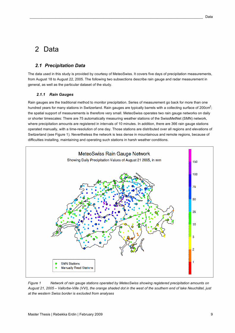
Rain gauges are the traditional method to monitor precipitation. Series of measurement go back for more than one
hundred years for many stations in Switzerland. Rain gauges are typically barrels with a collecting surface of 200cm2;
the spatial support of measurements is therefore very small. MeteoSwiss operates two rain gauge networks on daily
or shorter timescales: There are 75 automatically measuring weather stations of the SwissMetNet (SMN) network,
where precipitation amounts are registered in intervals of 10 minutes. In addition, there are 366 rain gauge stations
operated manually, with a time-resolution of one day. Those stations are distributed over all regions and elevations of
Switzerland (see Figure 1). Nevertheless the network is less dense in mountainous and remote regions, because of
difficulties installing, maintaining and operating such stations in harsh weather conditions.
Figure 1 Network of rain gauge stations operated by MeteoSwiss showing registered precipitation amounts on
August 21, 2005 – Vallorbe-Ville (VVI), the orange shaded dot in the west of the southern end of lake Neuchâtel, just
at the western Swiss border is excluded from analyses
Combining Rain Gauge and Radar Measurements of a Heavy Precipitation Event over Switzerland ______________
10 MeteoSwiss and ETH Zürich, D-MATH, Seminar for Statistics
Rain gauges are fairly accurate in absolute values. There are some systematic biases, as Sevruk (1985) pointed out.
The main source of bias in our latitudes is the deformation of the wind field by the gauge, which leads to deviations of
small droplets or light frozen hydrometeors and therefore losses in the observed amount. In addition, there are losses
by evaporation and residual water at emptying. Rebound effects can lead to negative or positive biases. These
biases depend strongly on season, type and strength of precipitation and exposure of the station. For the precipita-
tion situation of our case study, measurement errors are expected to be well below 5%, because droplets are large
and liquid and there are no strong winds. Rain gauge measurements are therefore assumed to be precise values of
precipitation at their specific location in this study.
The disadvantage of rain gauges is their low spatial and temporal resolution. Precipitation varies at very small scales
spatially as well as temporally. As the spatial support of each station is extremely small, the uncertainty about
precipitation amounts between stations is high, even in a dense gauge network as the one of MeteoSwiss. Analysing
the heavy precipitation event of August 2005, Frei et al. (2008) for instance found relative uncertainties for point esti-
mates based on the gauge network of 20-40%. A huge increase of gauges, and therefore enormous expenses, would
be necessary to achieve the high spatial resolution required by hydrologists with gauge information only. The same
problem arises attempting to achieve better temporal resolution by gauge measurements only. Although MeteoSwiss
plans to further densify its automatic network, the large increase in automated stations needed is out of reach.
The rain gauge dataset used for the study presented here consists of daily precipitation sums of 440 rain gauge
stations. The daily precipitation sum of day d refers to the 24-hours sum from 06:00 UTC of day d till 06:00 UTC of
day d+1. One station of the manually operated network, VVI (Vallorbe-Ville) is excluded from analyses because of
implausible values.
2.1.2 Radar
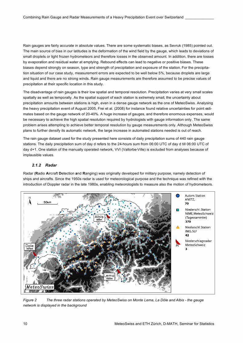
Radar (Radio Aircraft Detection and Ranging) was originally developed for military purpose, namely detection of
ships and aircrafts. Since the 1950s radar is used for meteorological purpose and the technique was refined with the
introduction of Doppler radar in the late 1980s, enabling meteorologists to measure also the motion of hydrometeors.
Figure 2 The three radar stations operated by MeteoSwiss on Monte Lema, La Dôle and Albis - the gauge
network is displayed in the background
_______________________________________________________________________________________ Data
Master Thesis | Rebekka Erdin | February 2009 11
The underlying principle is to send out electromagnetic wave pulses and measure the backscatter. The registered
backscattered power can be converted to radar reflectivity Z under the assumption of a given drop size distribution
(Marshall et al., 1947). This radar reflectivity can then be transformed into a rain rate R with a Z-R relation of the form
Z = a * R b. This is currently done with a fixed Z-R relation Z = 316 * R
1.5 at MeteoSwiss (Germann et al., 2006).
MeteoSwiss operates three C-band radars on the top of La Dôle in western Switzerland, Albis near Zürich and Monte
Lema in Ticino (see Figure 2). They cover the area of Switzerland with a resolution of five minutes and 1km
(MeteoSchweiz, 2006). This high temporal and spatial resolution is the strongest advantage of radar precipitation
measurement. Its limitation on the other hand, is a low accuracy of absolute values for several reasons as described
by Germann et al. (2006): The definition of the Z-R-relationship leads inevitably to errors due to variations in drop
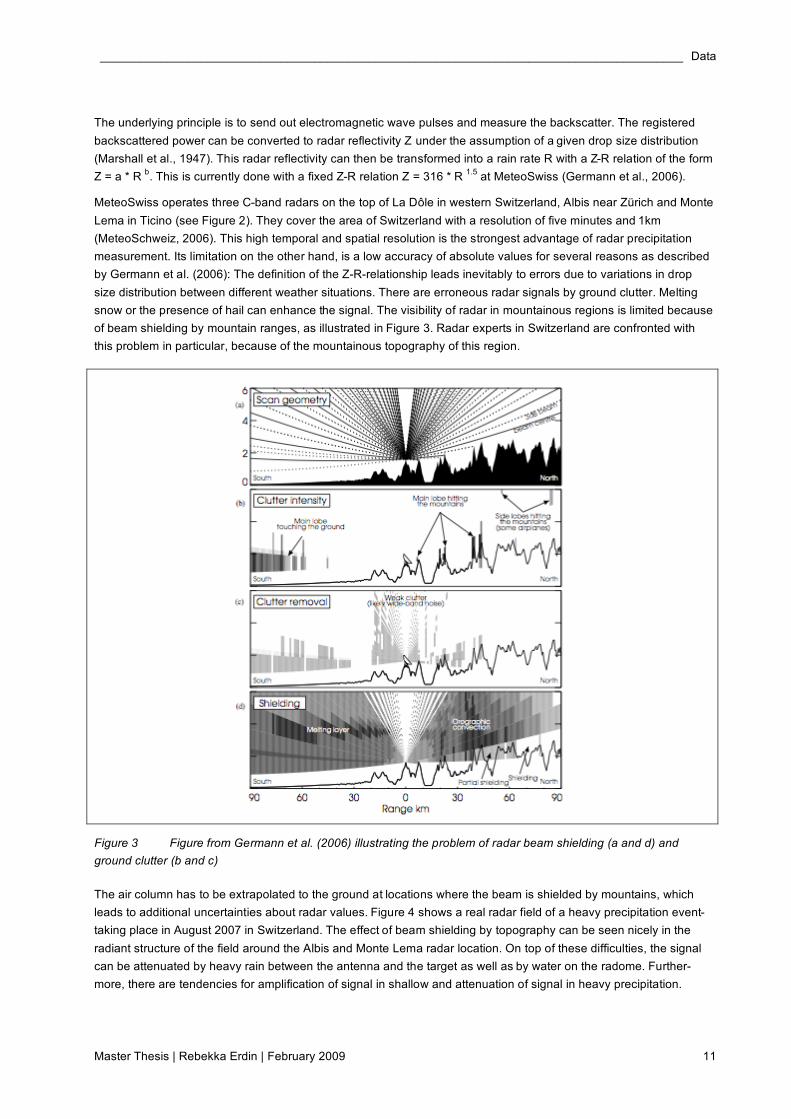
size distribution between different weather situations. There are erroneous radar signals by ground clutter. Melting
snow or the presence of hail can enhance the signal. The visibility of radar in mountainous regions is limited because
of beam shielding by mountain ranges, as illustrated in Figure 3. Radar experts in Switzerland are confronted with
this problem in particular, because of the mountainous topography of this region.
Figure 3 Figure from Germann et al. (2006) illustrating the problem of radar beam shielding (a and d) and
ground clutter (b and c)
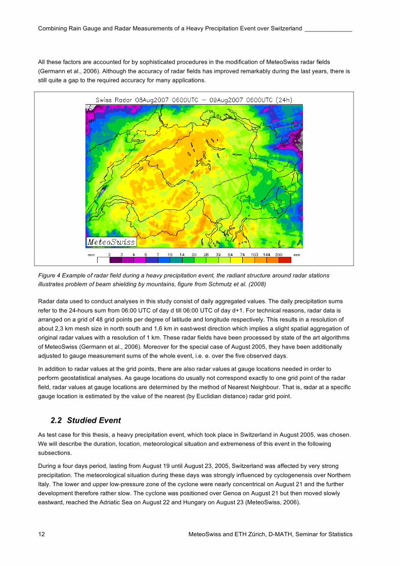
The air column has to be extrapolated to the ground at locations where the beam is shielded by mountains, which
leads to additional uncertainties about radar values. Figure 4 shows a real radar field of a heavy precipitation event-
taking place in August 2007 in Switzerland. The effect of beam shielding by topography can be seen nicely in the
radiant structure of the field around the Albis and Monte Lema radar location. On top of these difficulties, the signal
can be attenuated by heavy rain between the antenna and the target as well as by water on the radome. Further-
more, there are tendencies for amplification of signal in shallow and attenuation of signal in heavy precipitation.
Combining Rain Gauge and Radar Measurements of a Heavy Precipitation Event over Switzerland ______________
12 MeteoSwiss and ETH Zürich, D-MATH, Seminar for Statistics
All these factors are accounted for by sophisticated procedures in the modification of MeteoSwiss radar fields
(Germann et al., 2006). Although the accuracy of radar fields has improved remarkably during the last years, there is
still quite a gap to the required accuracy for many applications.
Figure 4 Example of radar field during a heavy precipitation event, the radiant structure around radar stations
illustrates problem of beam shielding by mountains, figure from Schmutz et al. (2008)
Radar data used to conduct analyses in this study consist of daily aggregated values. The daily precipitation sums
refer to the 24-hours sum from 06:00 UTC of day d till 06:00 UTC of day d+1. For technical reasons, radar data is
arranged on a grid of 48 grid points per degree of latitude and longitude respectively. This results in a resolution of
about 2,3 km mesh size in north south and 1,6 km in east-west direction which implies a slight spatial aggregation of
original radar values with a resolution of 1 km. These radar fields have been processed by state of the art algorithms
of MeteoSwiss (Germann et al., 2006). Moreover for the special case of August 2005, they have been additionally
adjusted to gauge measurement sums of the whole event, i.e. e. over the five observed days.
In addition to radar values at the grid points, there are also radar values at gauge locations needed in order to
perform geostatistical analyses. As gauge locations do usually not correspond exactly to one grid point of the radar
field, radar values at gauge locations are determined by the method of Nearest Neighbour. That is, radar at a specific
gauge location is estimated by the value of the nearest (by Euclidian distance) radar grid point.
2.2 Studied Event
As test case for this thesis, a heavy precipitation event, which took place in Switzerland in August 2005, was chosen.
We will describe the duration, location, meteorological situation and extremeness of this event in the following
subsections.
During a four days period, lasting from August 19 until August 23, 2005, Switzerland was affected by very strong
precipitation. The meteorological situation during these days was strongly influenced by cyclogenensis over Northern
Italy. The lower and upper low-pressure zone of the cyclone were nearly concentrical on August 21 and the further
development therefore rather slow. The cyclone was positioned over Genoa on August 21 but then moved slowly
eastward, reached the Adriatic Sea on August 22 and Hungary on August 23 (MeteoSwiss, 2006).
_______________________________________________________________________________________ Data
Master Thesis | Rebekka Erdin | February 2009 13
As the air reaching Central Europe was transported over the warm Mediterranean Sea, air humidity was high, which
is one of the reasons for the extraordinary high precipitation amounts observed. It can be shown by simulation
(MeteoSwiss, 2006), that the topography of the Alpine region was another crucial factor for the large amounts of
precipitation. The mountain range was leading to orographic uplift and blocking of low-level air masses. The fact that
the soil was already saturated with water at the beginning of the episode because of frequent precipitation in the
precedent days, amplified the hydrological impact of the precipitation event.
While August 18, 19 and 20 were dominated by convective precipitation and some thunder storms, the following days
were governed by heavy stratiform precipitation, first mainly over the Bernese Oberland and Central Switzerland,
then propagating more and more eastward, striking also Eastern Switzerland and Grisons. The main section of
precipitation was registered on August 21 and 22, when an accumulation situation north of the Alps was observed.
The long duration of the episode led to extreme 48-hours-sums at many stations, while the 24-hours-sums where
less exceptional. 28 stations for instance registered 48-hours-sums with an estimated return period of more than 50
years. On August 23, only the eastern part of Switzerland was still registering precipitation and the episode ended on
that day, as the cyclone and precipitation field moved further east (MeteoSwiss, 2006).
The heavy precipitation and flooding event of August 2005 has been extensively analysed by several institutions
(MeteoSwiss, 2006; Frei et al., 2008; Bezzola and Hegg, 2007 and 2008).

Combining Rain Gauge and Radar Measurements of a Heavy Precipitation Event over Switzerland ______________
14 MeteoSwiss and ETH Zürich, D-MATH, Seminar for Statistics
____________________________________________________________________________________ Methods
Master Thesis | Rebekka Erdin | February 2009 15
3 Methods
This section introduces the methodology of the thesis at hand. The first subsection describes how precipitation data
is transformed prior to analyses. The second subsection gives a short introduction into geostatistical concepts and
methods. Specific methods applied in this study and references to previous applications in literature can be found in
the third subsection. Evaluation methods including validation technique, reference and skill measures are described
in subsection four. The fifth and last subsection finally mentions the software used.
3.1 Transformation of Data
As for many statistical analyses, data is assumed to be of Gaussian distribution with mean µ and variance !2 for
model-based geostatistical methods (Diggle and Ribeiro, 2007). Real data, however, often exhibits distributions other
than Gaussian. Precipitation data in particular, is always positive-valued and positively skewed.
The Gaussian model can be extended in such a way, that data is assumed to be of Gaussian distribution after
applying an adequate transformation. Box and Cox (1964) introduced a useful and nowadays well-established class
of transformations to transform positive-valued, skewed data to approximately Gaussian distribution, the Box-Cox
family of transformations. These transformations depend on one additional parameter " and are of the form:
Y* = (Y" - 1) / " for " ! 0
Y* = log Y for " = 0
For our application primarily the assumption of Gaussian distribution of the residuals of the linear relationship
between radar and gauge data is needed (see section 3.3). To choose suitable values for lambda to transform our
data, we assess the distribution of those residuals of each day for three different lambdas:
" = 0, which equals to a log transformation
" = 0.5, which equals to a square root transformation
" = 0.23 which optimizes the likelihood of Gaussian distribution of residuals for observations of all five days
The third lambda (" = 0.23), fitted to the residuals of the entire examined event, is calculated as follows. The Profile
log-likelihood for Gaussian distribution of residuals of the linear relationship between Box-Cox transformed radar and
Box-Cox transformed gauge data is calculated for fixed values of lambda on the interval [-2,2] in steps of 0.01 (see
section 4.1). The maximum of this Profile log-likelihood values is chosen as possible lambda because the assumption
of Gaussian residuals is most likely in this case. The log and square root transformation are chosen because of their
theoretical meaningfulness.
In order to get precipitation fields and predictions at station locations for validation on the scale of actually observed
precipitation, back transformation of predictions is necessary. In doing so, we have to account for the fact that for
nonlinear transformations, the expected value on back transformed scale is usually not the same as the inverse
transformation of the expected value on transformed scale. Simple back transformation of the estimated expected
value by the inverse Box-Cox transformation would therefore lead to biased estimates. Hence more sophisticated
back transformation methods are required in order to get unbiased estimates of expected values. Diggle and Ribeiro
(2007) point out that this can be done analytically for the " = 0 (the log transformation) and " = 0.5 (the square root
transformation), but not for other values of " for the Box-Cox transformation. In this case, back transformation is
performed by simulating from the predicted Gaussian distribution at a prediction location and transforming the simula-
ted values back. This yields a sample of the predictive distribution on the scale of real precipitation and its mean can
be taken as prediction at this specific location. The analytical and Monte Carlo method for back transformation
Combining Rain Gauge and Radar Measurements of a Heavy Precipitation Event over Switzerland ______________
16 MeteoSwiss and ETH Zürich, D-MATH, Seminar for Statistics
depending on " as described above is implemented in the R package geoR (Ribeiro and Diggle, 2001), which was
used for this study. We perform 1000 simulations per prediction for Monte Carlo back transformations.
3.2 Geostatistical Methods
This section introduces the general concept and methods of geostatistics. It is based on lecture notes for an
introductory course in statistical modelling of spatial data (Papritz, 2008) as well as books published on the topic
(Cressie, 1993; Diggle and Ribeiro, 2007; Webster and Oliver, 2007). The introduction is done in a summarizing way,
making no claim to be complete, but with the idea of helping an unfamiliar reader to understand the following sections
of this study. For more details, we refer to the literature mentioned above.
If we analyse data with spatial reference, meaning that each observation Yi refers to a one, two or three dimensional
vector si, specifying a point in space where this observation is located, the usual assumption of independence of data
is typically violated. This offers a particular challenge to applied methods, but also particular possibilities for
predictions between observed data points.
If all influences on a target variable were deterministic and perfectly known, the variable could be predicted in
continuous space with absolute accuracy. In most cases, however, influencing processes and dependencies are not
understood in every detail. In this situation a stochastic concept, such as statistical methods for spatial data, is very
helpful. The models for spatial data define mean, variance and spatial covariance structure of the data. This
approach is called the theory of regionalized variables: The dataset of n spatially referenced data points is perceived
as one realisation of a multivariate random variable, whose characteristics are determined by a parametric model.
The spatial index s of geostatistical data can vary continuously in the observed area and the distances between data
points are usually irregular.
Important for geostatistical methods is the assumption of stationarity. It can be relaxed to the assumption of weak
stationarity for most applications, meaning that the expectation #{Y(si)} and variance var{Y(si)} are constant for all i
and the covariance cov{Y(si)-Y(sj)} only depends on the lag h = ||si – sj|| (Euclidean distance between si and sj), but
not on the positions in space of si and sj. There are different terms to describe the autocovariance or autocorrelation
of a spatially referenced variable Y:
• The Autocovariance C(h) = E{(Y(s+h) – E{Y(s+h)}} * E{(Y(s) – E{Y(s)}}
• The Auto-Correlation r(h) = C(h) / Var(Y)
• The Semivariance $(h) = (1/2) * #{(Y(s + h) – Y(s))2}
This autocorrelation structure is traditionally characterised by the semivariance $(h) in geostatistical contexts. $(h) as
a function of h is called the semivariogram. As it is usually simply referred to as variogram in the literature, we will
term it this way in the following. The covariance structure of geostatistical data is usually such that data points lying
close to each other are positively correlated, i.e. the semivariance for a small lag is smaller than the semivariance for
a bigger lag.
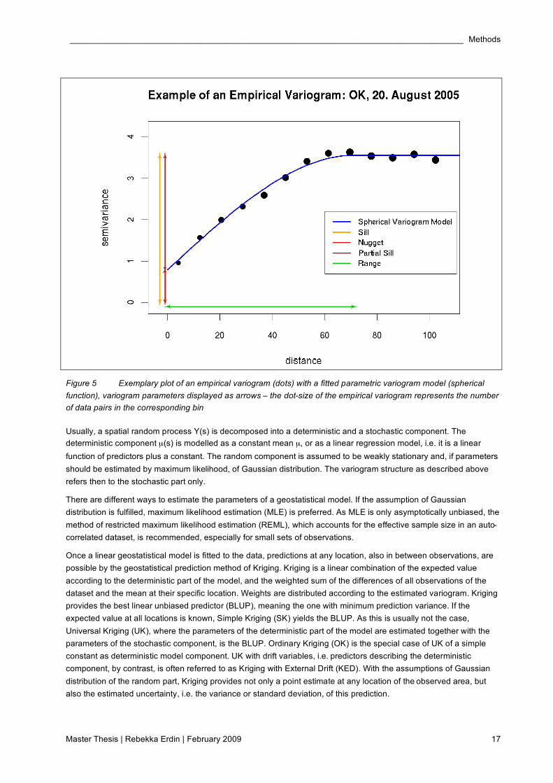
It is common to merge all observed data pairs into bins of lag distances with a fixed band width, h±%h for plots of the
empirical variogram in order to get a signal of $(h) without too much random noise (see Figure 5). For some situations
it is advisable to model anisotropic (i.e. direction dependent) variograms. As we did not use this method in our study,
this will not be explained here.
The semivariance is modelled parametrically by a convenient parametric function that fulfils certain requirements
imposed by the assumption of stationarity and other mathematical conditions. There are several established functions
for variogram modelling, most of them including parameters for the sill or partial sill, the nugget and the range of the
variogram, as illustrated in Figure 5. Some models include an additional parameter &, defining the
roughness/smoothness of the spatial distribution of observations. The spherical and exponential models used in our
study however do not include a roughness parameter.
____________________________________________________________________________________ Methods
Master Thesis | Rebekka Erdin | February 2009 17
Figure 5 Exemplary plot of an empirical variogram (dots) with a fitted parametric variogram model (spherical
function), variogram parameters displayed as arrows – the dot-size of the empirical variogram represents the number
of data pairs in the corresponding bin
Usually, a spatial random process Y(s) is decomposed into a deterministic and a stochastic component. The
deterministic component µ(s) is modelled as a constant mean µ, or as a linear regression model, i.e. it is a linear
function of predictors plus a constant. The random component is assumed to be weakly stationary and, if parameters
should be estimated by maximum likelihood, of Gaussian distribution. The variogram structure as described above
refers then to the stochastic part only.
There are different ways to estimate the parameters of a geostatistical model. If the assumption of Gaussian
distribution is fulfilled, maximum likelihood estimation (MLE) is preferred. As MLE is only asymptotically unbiased, the
method of restricted maximum likelihood estimation (REML), which accounts for the effective sample size in an auto-
correlated dataset, is recommended, especially for small sets of observations.
Once a linear geostatistical model is fitted to the data, predictions at any location, also in between observations, are
possible by the geostatistical prediction method of Kriging. Kriging is a linear combination of the expected value
according to the deterministic part of the model, and the weighted sum of the differences of all observations of the
dataset and the mean at their specific location. Weights are distributed according to the estimated variogram. Kriging
provides the best linear unbiased predictor (BLUP), meaning the one with minimum prediction variance. If the
expected value at all locations is known, Simple Kriging (SK) yields the BLUP. As this is usually not the case,
Universal Kriging (UK), where the parameters of the deterministic part of the model are estimated together with the
parameters of the stochastic component, is the BLUP. Ordinary Kriging (OK) is the special case of UK of a simple
constant as deterministic model component. UK with drift variables, i.e. predictors describing the deterministic
component, by contrast, is often referred to as Kriging with External Drift (KED). With the assumptions of Gaussian
distribution of the random part, Kriging provides not only a point estimate at any location of the observed area, but
also the estimated uncertainty, i.e. the variance or standard deviation, of this prediction.

Combining Rain Gauge and Radar Measurements of a Heavy Precipitation Event over Switzerland ______________
18 MeteoSwiss and ETH Zürich, D-MATH, Seminar for Statistics
3.3 Specific Methods Compared in this Study
All methods applied in this study are geostatistical approaches as introduced above (see section 3.2). Most of them
have been described in literature to generate precipitation fields, but none of them was conducted in Switzerland. In
the following subsections, these methods and their adaptation to this case study are explained in more detail. We use
the following notation
Y rain gauge measurements
X radar measurements
R radar errors
U radar uncertainty
Z modelled precipitation amount
j as index for one of n gauge stations
s as the spatial reference of a grid point, referred to by index i
3.3.1 Kriging of Radar Errors
The idea of this approach is to interpolate the error of radar values and then subtract this interpolated field of radar
error from the observed radar field to get the predicted field. Radar errors (R) are determined by comparison of radar
measurements (X) with gauge measurement (Y) at gauge location j, which are regarded as true precipitation values
at their specific location in this study, as follows:
Rj = Yj - Xj
The modelled precipitation amount at any grid point si is the sum of the radar measurement and the radar error at
that location:
Z(si) = X(si) + R(si)
The predicted field is by definition perfectly consistent with gauge measurements at all gauge locations.
DeGaetano and Wilks (2008) applied this method to precipitation data in Eastern US. The difference between their
approach and the approach of this study is that they interpolate the field of radar errors by Inverse-distance-weighting
(IDW), whereas we apply Ordinary Kriging (OK). We prefer OK, because in contrast to IDW, it accounts for the
specific spatial covariance structure of radar errors, which can vary significantly between different precipitation
situations. A different approach resulting in the same precipitation fields, can be found in Jurczyk et al. (2007). Their
approach is to determine the error of interpolation. This is done by the interpolation of only those radar values located
at a gauge station and the comparison of this interpolated field with the real radar field. The resulting interpolation
error is then subtracted from the interpolated gauge field. Jurczyk et al. (2007) compared both, Kriging and IDW, in
their study and found that they were comparable in terms of results.
In this study, we perform OK of radar errors with transformed data, as described in section 3.1. Predicted fields and
values at gauge locations are then back transformed as described in section 3.1, in order to get comparable fields
and cross validation errors.
Variograms are modelled by the exponential or the spherical function. The function is chosen in order to get a good
representation of the empirical variogram by the model. Variogram models are fitted to the data by Restricted
Maximum Likelihood Estimation (REML).
____________________________________________________________________________________ Methods
Master Thesis | Rebekka Erdin | February 2009 19
3.3.2 Kriging with External Drift
In this approach, Kriging with external drift (KED) with radar as external drift variable is applied, i.e. the precipitation
amount Z at a location si is modelled by:
Z(si) = ' + (Y(si) + )(si)
Where the first two terms on the right-hand side define the deterministic part of the model and )(si) denotes for the
part of the model based on the observed autocovariance structure for the prediction location si, which is determined
by the linear weighted sum of all observations as described in the section on Kriging (see 3.2). This offers more
flexibility than the Kriging of radar errors, because radar values are multiplied with a specific coefficient (, that needs
not to be exactly equal to one, and there is an additional intercept ' in the model. Haberlandt (2007) applied this
method with parametric variogram estimation to generate precipitation fields of a heavy precipitation event in
Germany. Velasco-Forero et al. (2004) suggested to estimate the variogram by a non-parametric method based on
Fast Fourier Transform (FFT) in order to be better implementable for real-time applications. As this is a case study,
and not an automated implementation, we apply conventional parametric variogram estimation.
Transformation of data, variogram modelling and parameter estimation are performed as described in the preceding
section on the Kriging of radar errors (see 3.3.1).
3.3.3 Double Optimal Estimation (DOE)
Barancourt et al. (1992) proposed the idea, to separate the modelling of wet/dry areas from the modelling of the
amount of precipitation in rainy areas. While their approach is based on rain gauge measurements only, Seo (1998)
applied the same idea combining rain gauge and radar measurements. Both authors perform independent
estimations of the probability of precipitation and the amount of precipitation given that positive precipitation at this
location is observed (conditional expectation).
It was originally planned to implement the DOE method in this case study and some preliminary experiments have
actually been undertaken. However further theoretical considerations and practical experience let us abandon this
idea. The procedure proposed by Seo (1998) makes several assumptions about the identity of different conditional
expectations. These do not necessarily hold in a spatially autocorrelated environment; moreover the inclusion of all
observations (including dry stations) for the modelling of the conditional expectation results in a biased estimation. An
alternative procedure, namely to model the probability of precipitation by Indicator Kriging (IK) and the conditional
expectation of precipitation amounts with KED, both with radar as spatial trend variable, has the following theoretical
deficiencies. As Papritz et al. (2005) show, Indicator Kriging (IK) with a spatial trend, which would be needed for the
estimation of the probability of precipitation, would require the modelling of a non-stationary variogram. As this is not
possible with only one realization of our regionalized variable, the procedure lacks optimality. In addition, compared
to the estimation of the unconditional expectation, the estimation of the conditional expectation by KED results in
substantially smaller coefficients in the spatial trend (radar), because dry stations are not included in this Kriging step.
This is especially the case for days with considerable amount of dry stations, e.g. the coefficient of radar decreases
from 0.55 to 0.45 on August 18 and from 0.55 to 0.50 on August 19 (for " = 0.5, the exponential variogram model and
the full station dataset). This leads to unsatisfactory results in the estimated field of conditional expectation. For
instance, there are regions where the conditional expectation is smaller than the unconditional expectation. And in
some cases, values of conditional expectation are even below the threshold chosen to separate wet from dry areas.
We still consider the idea of separating the factor wet/dry from the amount of precipitation as an interesting option,
because it offers a possibility to handle the specific distribution of precipitation with its frequent peak at zero. Yet the
theoretical concepts for such an approach need further development for models with an external trend variable.
Combining Rain Gauge and Radar Measurements of a Heavy Precipitation Event over Switzerland ______________
20 MeteoSwiss and ETH Zürich, D-MATH, Seminar for Statistics
3.3.4 Modelling Radar Uncertainty
To refine KED with radar as drift variable, we attempt to model the quality of radar information and introduce this
additional information to our model. This is done by the introduction of a variable radar uncertainty (U) and their
interaction with radar measurements (X) into the deterministic part of the model:
Z(si) = ' + (1Y+ (2U + (3YU+ )i
The influence of U on Z has no physical meaning. Depending on the precipitation situation (2 is expected to be of
positive or negative sign and varying size. But we include U because we are interested in the interaction term YU and
the sign of (3. The theory of errors-in-variables (Stahel, 2006) explains that the slope of a linear relation between a
predictor and a target variable is less steep if the predictor is tainted with a larger uncertainty. A negative (3 implies
that for larger values of U the coefficient (1 is reduced. This means that the slope of the linear dependence of Z from
Y is less steep, which would be the case for radar values with larger uncertainty.
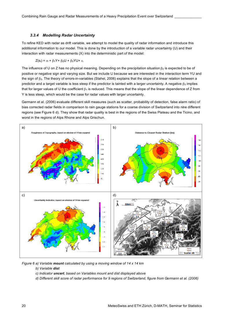
Germann et al. (2006) evaluate different skill measures (such as scatter, probability of detection, false alarm ratio) of
bias corrected radar fields in comparison to rain gauge stations for a coarse division of Switzerland into nine different
regions (see Figure 6 d). They show that radar quality is best in the regions of the Swiss Plateau and the Ticino, and
worst in the regions of Alps Rhone and Alps Grischun.
a)
b)
c)
d)
Figure 6 a) Variable mount calculated by using a moving window of 14 x 14 km
b) Variable dist
c) Indicator uncert, based on Variables mount and dist displayed above
d) Different skill score of radar performance for 9 regions of Switzerland, figure from Germann et al. (2006)

____________________________________________________________________________________ Methods
Master Thesis | Rebekka Erdin | February 2009 21
In this study we attempt to model the distribution of radar quality by two variables – the distance to the closest radar
station (dist) and the roughness of topography (mount). Figure 6 shows that this is a fair approximation of the pattern
found by Germann et al. (2006).
Variable mount (Figure 6 a) is modelled as the local standard deviation of topography. This is done by calculating the
standard deviation of all grid points within a moving square window of 14 km edge length centred at the specific grid
point.
Variable dist (Figure 6 b) is modelled as the simple Euclidean distance from each grid point to the closest radar
station. For simplicity reasons the proportion of degrees longitude and latitude is assumed to be constant over
Switzerland.
The variables mount and dist and their interaction terms with radar could be included as trend variables separately
into the model. For simplicity reasons we prefer to use one single uncertainty variable and its interaction with radar in
this study. For this purpose we merge the two variables dist and mount into an indicator variable for total radar
uncertainty (uncert). This is done by scaling both variables linearly down, such that they vary between 0 and 0.5, and
then adding them up. The resulting indicator variable uncert (Figure 6 c) lies by definition between 0 and 1 and the
variables dist and mount are each weighted fifty percent to determine the value of uncert at a specific location.
KED including the additional information of radar uncertainty is performed using the same methods as for KED
including only radar as drift variable (see section 3.3.2). The only difference is that the indicator uncert and the
interaction term between uncert and radar are additionally included to model the drift.
3.3.5 Further Additional Trend Variables
Furthermore, we tried to refine the KED with radar by three other additional trend variables during the course of this
study: height above sea level, climatological precipitation values of August and a non-parametric smoother. However,
none of them is further pursued, as they did not improve combined precipitation fields at all.
3.4 Evaluation and Reference
The comparison and evaluation of the performance of methods described in the preceding section is the main
purpose of this study. The following subsections describe how performance is evaluated. The first two subsections
explain two different validation settings to obtain errors of predictions by a method compared to gauge
measurements, which are considered as true values. The first one, cross validation, is done by including all gauge
stations in the model, while the second one is done by dividing the available gauge stations into a model and a test
data set. The last three subsections describe the further assessment of those prediction errors, once they are
determined, i.e. what they are compared to and how they are condensed to enable quantitative comparison.
3.4.1 Cross Validation
The concept of cross validation is well known and established in situations, where no test set of data is available to
assess the performance of a model. It is also frequently suggested in the geostatistical context (Cressie, 1993;
Webster and Oliver, 2007). The idea is to exclude one data point from the data set, fit the model to the remaining
data set and predict with this model at the location of the excluded data point. This prediction can then be compared
to the real observation at that location yielding the so-called cross validation error. This procedure is repeated for
each data point successively in order to get n cross validation errors to assess the predictive ability of the model.
The computational effort needed to perform a separate MLE to fit a geostatistical model for each of the 440
observations, five analysed days and different analysed methods is very large. A computationally less expensive
alternative is to fit one geostatistical model to all observations by MLE and repeat only the Kriging step with one
observation excluded from the dataset at a time. We therefore check by means of a few selected comparisons

Combining Rain Gauge and Radar Measurements of a Heavy Precipitation Event over Switzerland ______________
22 MeteoSwiss and ETH Zürich, D-MATH, Seminar for Statistics
whether the results of the two procedures show substantial differences. As results in Table 1 show, the differences
are tiny. The application of cross validation for Kriging, but not for model estimation, as performed in this study is
therefore well justified.
Table 1 Comparison of different skill scores (see section 3.4.4 for explanations of the scores) based on results
of overall cross validation including MLE and cross validation exclusively for Kriging for two example cases
Cross Validation day " variog Method hk rms.rel.start bias.sq rmse.sq made.sq
Full CV 18 0.5 exp OK 0.016 0.328 0.234 0.829 0.770
Kriging only 18 0.5 exp OK 0.016 0.325 0.234 0.824 0.769
Full CV 19 0.5 exp KEDradar 0.019 0.200 0.110 0.711 0.628
Kriging only 19 0.5 exp KEDradar 0.019 0.199 0.109 0.707 0.628
3.4.2 Test Data Validation
In this study, all analyses are performed on daily time scale. But many applications require precipitation fields of
shorter time scales. Therefore it will be important to apply methods able to cope with the less dense gauge network of
automatic (SMN) stations. To get an idea about the possible performance of the methods applied in this study, we
build models including only SMN stations for each method. The remaining manually operated stations can then be
used as independent test data in order to assess the quality of predictions.
3.4.3 Fields for Comparison
This study compares different geostatistical methods to combine rain gauge and radar measurements with each
other. In addition, combined fields are also compared to precipitation fields based only on gauge or radar data
respectively. This comparison to pure gauge and radar fields is important for several reasons. First of all, precipitation
fields based on gauge measurements only are used in most applications at the moment. The question whether
including the additional information of radar can improve precipitation fields and by how much, is therefore of interest.
Second, this comparison allows assessing differences in performance between methods relative to the added value
of the combination over pure gauge or radar fields. Last but not least, our aim is to combine the strengths of gauge
and radar measurements. We would therefore like to check, whether combination methods are able to reduce biases
substantially compared to radar fields as well as whether a higher spatial resolution is achieved compared to gauge
fields.
Hence, we compare our results from combination methods
• with each other
• to pure gauge fields
• to pure radar fields
For the field based on gauge measurements only (b), we perform OK. As for the combination methods, variograms
are modelled by exponential or spherical function. The function is chosen in order to get a good representation of the
empirical variogram by the model. Variogram models are fitted to the data by Restricted Maximum Likelihood
Estimation (REML) and predicted values are back transformed as described in section 3.1.
The radar field (c) can be used as such. Values at station locations to assess prediction errors are determined by the
Nearest Neighbour method (see section 2.1.2).
____________________________________________________________________________________ Methods
Master Thesis | Rebekka Erdin | February 2009 23
3.4.4 Skill Scores
Scalar measures are needed in order to condense, compare and assess the skill of different methods. The following
skill measures are calculated for each combination and pure field:
hk the Hanssen-Kuipers Discriminant (also called True Skill Statistic)
rel skill the Root Mean Square (RMS) of relative error
rmse.sq the Root Mean Squared Error (RMSE) of the difference between the square root of predictions
and the square root of observations
bias.sq the difference between the square root of predictions and the square root of observations
made.sq 1.4826 times the Median Absolute Deviation (MAD) of the difference between the square root
of predictions and the square root of observations
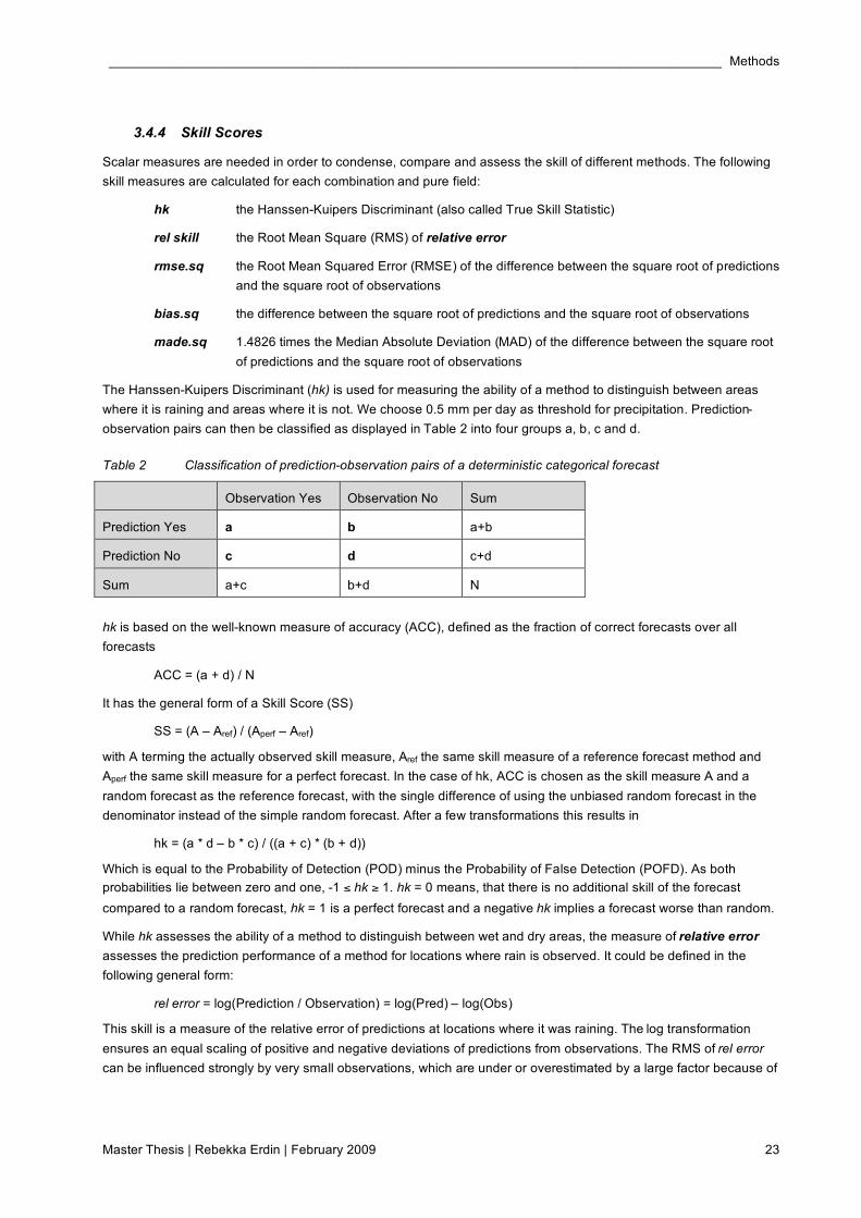
The Hanssen-Kuipers Discriminant (hk) is used for measuring the ability of a method to distinguish between areas
where it is raining and areas where it is not. We choose 0.5 mm per day as threshold for precipitation. Prediction-
observation pairs can then be classified as displayed in Table 2 into four groups a, b, c and d.
Table 2 Classification of prediction-observation pairs of a deterministic categorical forecast
Observation Yes Observation No Sum
Prediction Yes a b a+b
Prediction No c d c+d
Sum a+c b+d N
hk is based on the well-known measure of accuracy (ACC), defined as the fraction of correct forecasts over all
forecasts
ACC = (a + d) / N
It has the general form of a Skill Score (SS)
SS = (A – Aref) / (Aperf – Aref)
with A terming the actually observed skill measure, Aref the same skill measure of a reference forecast method and
Aperf the same skill measure for a perfect forecast. In the case of hk, ACC is chosen as the skill measure A and a
random forecast as the reference forecast, with the single difference of using the unbiased random forecast in the
denominator instead of the simple random forecast. After a few transformations this results in
hk = (a * d – b * c) / ((a + c) * (b + d))
Which is equal to the Probability of Detection (POD) minus the Probability of False Detection (POFD). As both
probabilities lie between zero and one, -1 * hk + 1. hk = 0 means, that there is no additional skill of the forecast
compared to a random forecast, hk = 1 is a perfect forecast and a negative hk implies a forecast worse than random.
While hk assesses the ability of a method to distinguish between wet and dry areas, the measure of relative error
assesses the prediction performance of a method for locations where rain is observed. It could be defined in the
following general form:
rel error = log(Prediction / Observation) = log(Pred) – log(Obs)
This skill is a measure of the relative error of predictions at locations where it was raining. The log transformation
ensures an equal scaling of positive and negative deviations of predictions from observations. The RMS of rel error
can be influenced strongly by very small observations, which are under or overestimated by a large factor because of
Combining Rain Gauge and Radar Measurements of a Heavy Precipitation Event over Switzerland ______________
24 MeteoSwiss and ETH Zürich, D-MATH, Seminar for Statistics
their small absolute value. To mitigate this property we use so-called “started logs” (st.log) proposed by Stahel
(personal communication, Dec 2008) instead of the common logarithmic function:
st.log(x) = log10 (x) for x > lc with lc = q0.25 * (q0.25 / q0.75)
st.log(x) = log10 (lc) + (x – lc) / (lc * ln(10)) for x * lc
lc defines the critical threshold: values smaller than this threshold are not logarithmized, but decreasing linearly in a
continuous and continuously differentiable function of x. lc is determined based on the first and third quartile of the
specific data. In our case we choose the quartiles of the total observations of all five days to determine lc in order to
get a single threshold for all days and therefore comparable skill scores. The resulting threshold is 1.2 mm. As not
small ratios, but small observations and predictions are to be mitigated, st.log has to be applied prior to ratio building:
rel error by started logs = st.log(Pred) – st.log(Obs)
This rel error is calculated for each pair of prediction and observation and then condensed to a scalar measure,
termed rms.rel.started in the following, by taking the root mean square (RMS) of the rel error of all observations.
In addition to the hk and rms.rel.started, which assess the ability of a method based on the separation into rain and
no-rain areas, we use also skill measures summarizing prediction features of all observations. In literature, most
authors use such summarizing skill measures on the scale of absolute precipitation values (deGaetano and Wilks,
2008; Haberlandt, 2007; Jurczyk et al., 2007; Seo, 1998; Velasco-Forrero et al., 2004). The disadvantage of this
approach is that the values of different cases are hardly comparable between days, because the predictability of
precipitation depends strongly on the average precipitation amount observed. We thus assess skill measures on
transformed scales in this study in order to achieve better comparability between the five different days of our event.
We choose 0.5 as one feasible lambda for the Box-Cox transformation of our precipitation data (see section 4.1).
This corresponds to a square root transformation of data. We therefore assess some well-known skill measures on
the scale of square root transformed predictions and observations – bias, rmse and made, defined as follows:
bias.sq = (-1 / n) , (Pred’ – Obs’)
rmse.sq = sqrt( (1 / n) , (Pred’ – Obs’)2)
made.sq = 1.4826 * Median (|Pred’ – Obs’|)
Where ‘ denotes square root transformed values. Negative predictions are set to zero prior to the square root
transformation. This is done on the one hand, because negative predictions make no sense for theoretical reasons,
as precipitation amounts are always non-negative. On the other hand, because of the fact that the square root
transformation can only be applied to non-negative values.
made is an estimate for the standard deviation as rmse, but more robust because it uses the median instead of the
mean and the absolute deviation instead of the squared deviation.
3.4.5 ANOVA
There are several factors (see Table 3) that could potentially influence prediction quality. Beside the different
methods as described in section 3.3, these are the density of the gauge network (see 3.4.1 and 3.4.2), the
precipitation characteristics of the examined day, the two different lambdas chosen to transform data prior to analysis
(see section 4.1) and the function chosen to model the variogram. To examine which of these factors have a
significant influence on the results in our case study, we perform Analyses of Variance (ANOVA). Different skill
scores as described in 3.4.4 serve as target variables and the factors described above are considered as influencing
variables for these analyses. ANOVA compares the variability of the target variable within the groups of an
influencing factor, to the variability between those groups, in order to assess whether this factor has a significant
influence on the target variable. The method belongs to the class of linear models and is well established and
described in statistical literature. It will therefore not be further explained here, please refer to statistical books, e.g.
Stahel (2008), for details. The variables dens, lambda, variog and rad are considered as fixed effects, i.e. they can be
____________________________________________________________________________________ Methods
Master Thesis | Rebekka Erdin | February 2009 25
repeated for further experiments. Beside these four main effects, the interaction between dens and rad is included as
additional fixed effect in our models. We will use the same notation for interaction terms as common model formulas
in R - variable1:variable2 – in the following. The interaction between dens and rad is denoted by dens:rad, as an
example according to this notation. Other possible interactions between fixed effects are not considered, as they are
not expected from theoretical point of view and did not show significant influence in a few selected test models
including them. The variable day is a random effect, i.e. its categories cannot be reproduced in further applications.
We are therefore faced with a mixed effect model, which has to be considered in model building for the ANOVA. day
and its interactions with other effects, which are all considered possibly meaningful, are included into the model as a
grouping variable. This means, we are not interested in their specific coefficients, but in the fact, whether the
influence of the grouping of observations by their categories is significant or not and what proportion of the remaining
variance they are explaining. To assess whether this random effects have a significant influence and should therefore
be included into the model, we perform Likelihood-Ratio-Tests of nested design models, one including the specific
random effect, the other not. Tuckey Anscombe Plots, showing the residuals of the model by the fitted model value
and QQ-Normal Plots of the residuals are examined to assess model assumptions.
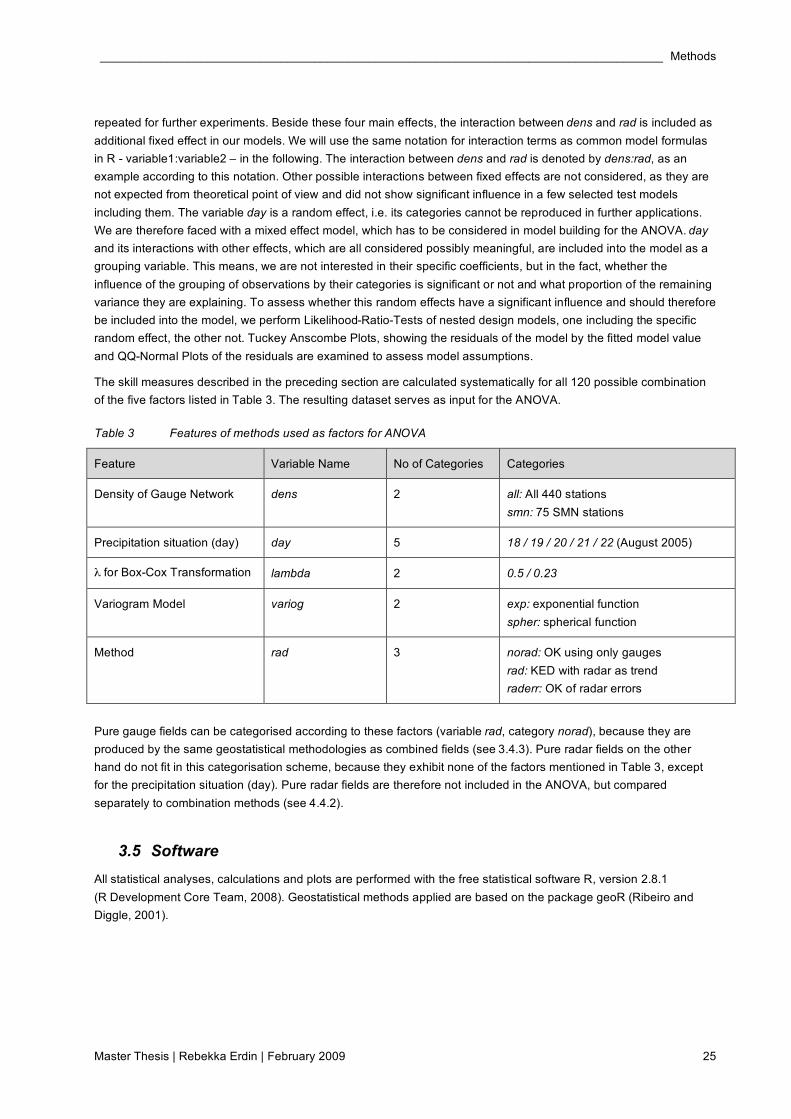
The skill measures described in the preceding section are calculated systematically for all 120 possible combination
of the five factors listed in Table 3. The resulting dataset serves as input for the ANOVA.
Table 3 Features of methods used as factors for ANOVA
Feature Variable Name No of Categories Categories
Density of Gauge Network dens 2 all: All 440 stations
smn: 75 SMN stations
Precipitation situation (day) day 5 18 / 19 / 20 / 21 / 22 (August 2005)
" for Box-Cox Transformation lambda 2 0.5 / 0.23
Variogram Model variog 2 exp: exponential function
spher: spherical function
Method rad 3 norad: OK using only gauges
rad: KED with radar as trend
raderr: OK of radar errors
Pure gauge fields can be categorised according to these factors (variable rad, category norad), because they are
produced by the same geostatistical methodologies as combined fields (see 3.4.3). Pure radar fields on the other
hand do not fit in this categorisation scheme, because they exhibit none of the factors mentioned in Table 3, except
for the precipitation situation (day). Pure radar fields are therefore not included in the ANOVA, but compared
separately to combination methods (see 4.4.2).
3.5 Software
All statistical analyses, calculations and plots are performed with the free statistical software R, version 2.8.1
(R Development Core Team, 2008). Geostatistical methods applied are based on the package geoR (Ribeiro and
Diggle, 2001).

Combining Rain Gauge and Radar Measurements of a Heavy Precipitation Event over Switzerland ______________
26 MeteoSwiss and ETH Zürich, D-MATH, Seminar for Statistics
_____________________________________________________________________________________ Results
Master Thesis | Rebekka Erdin | February 2009 27
4 Results
Results of our case study are presented in this section. The first subsection discusses the results of our investiga-
tions about different transformations of data prior to analysis. Typical features of variograms fitted to our data are
discussed in subsection two. We examine situations systematically by varying five different factors (dens, day,
lambda, variog and rad) as described in section 3.4.5. Subsection three describes the results of the ANOVA based
on these five factors performed with different skill scores as target variables. This section should help to get an
overview of influences and relations of different factors. Subsection four focuses on the comparison between pure
gauge and pure radar fields with combined precipitation fields. This is done by additional analyses and example
cases to illustrate qualitative differences. Similar analyses and examples are discussed in subsection five for the
comparison between the two different combination methods. Subsection six finally describes the results of
combination methods including an additional variable modelling radar uncertainty.
4.1 Box-Cox Transformation
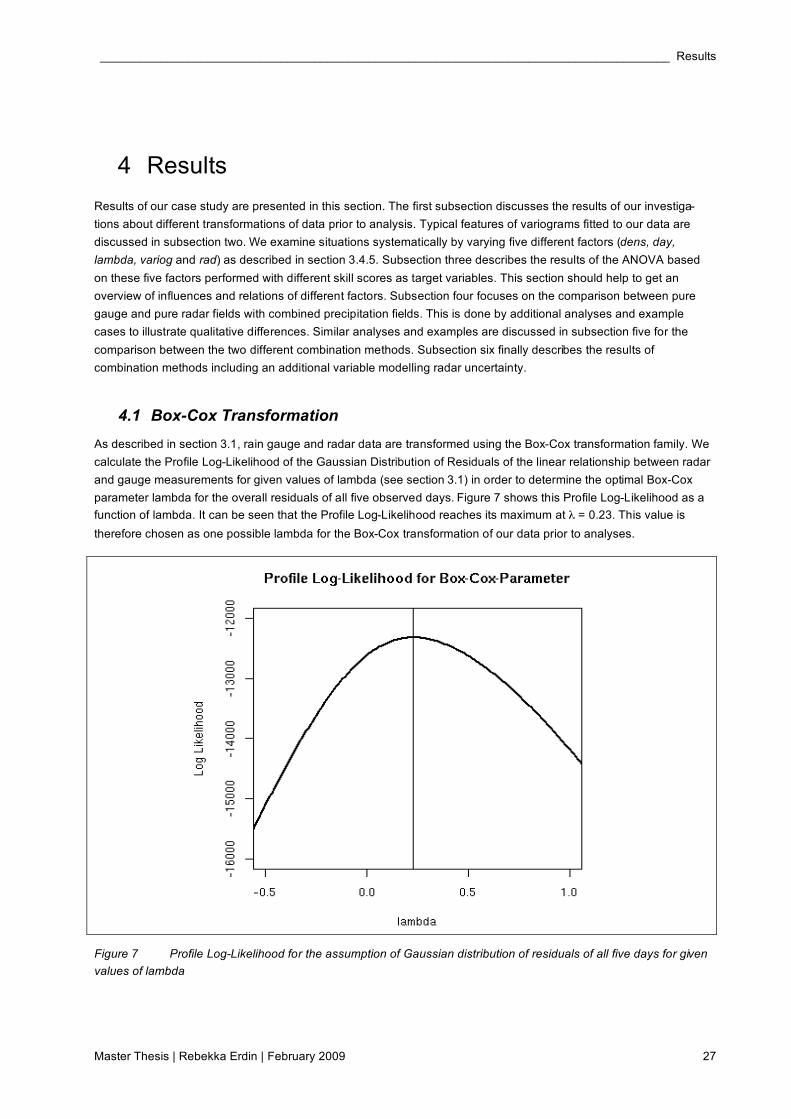
As described in section 3.1, rain gauge and radar data are transformed using the Box-Cox transformation family. We
calculate the Profile Log-Likelihood of the Gaussian Distribution of Residuals of the linear relationship between radar
and gauge measurements for given values of lambda (see section 3.1) in order to determine the optimal Box-Cox
parameter lambda for the overall residuals of all five observed days. Figure 7 shows this Profile Log-Likelihood as a
function of lambda. It can be seen that the Profile Log-Likelihood reaches its maximum at " = 0.23. This value is
therefore chosen as one possible lambda for the Box-Cox transformation of our data prior to analyses.
Figure 7 Profile Log-Likelihood for the assumption of Gaussian distribution of residuals of all five days for given
values of lambda
Combining Rain Gauge and Radar Measurements of a Heavy Precipitation Event over Switzerland ______________
28 MeteoSwiss and ETH Zürich, D-MATH, Seminar for Statistics
As described in section 3.1 we assess the fit of the residuals to Gaussian distribution for the square root (" = 0.5) and
the logarithmic (" = 0) transformation beside this optimized value of lambda. QQ-Normal-Plots and plots of residuals
against radar values at gauge locations for all three choices of lambda and for all five days (see Appendix section
10.1) show that the log transformation is not very adequate for all days except for August 18. The square root trans-
formation and the transformation with " = 0.23 are in general quite suitable for all days. The square root transforma-
tion exhibits a less suitable fit for August 18 and the transformation with " = 0.23 for August 21 than the other days or
transformations. However, their deviations from constant variance and Gaussian distributions are not too severe. We
therefore perform our analyses with Box-Cox transformed data systematically with both, " = 0.5 and " = 0.23.
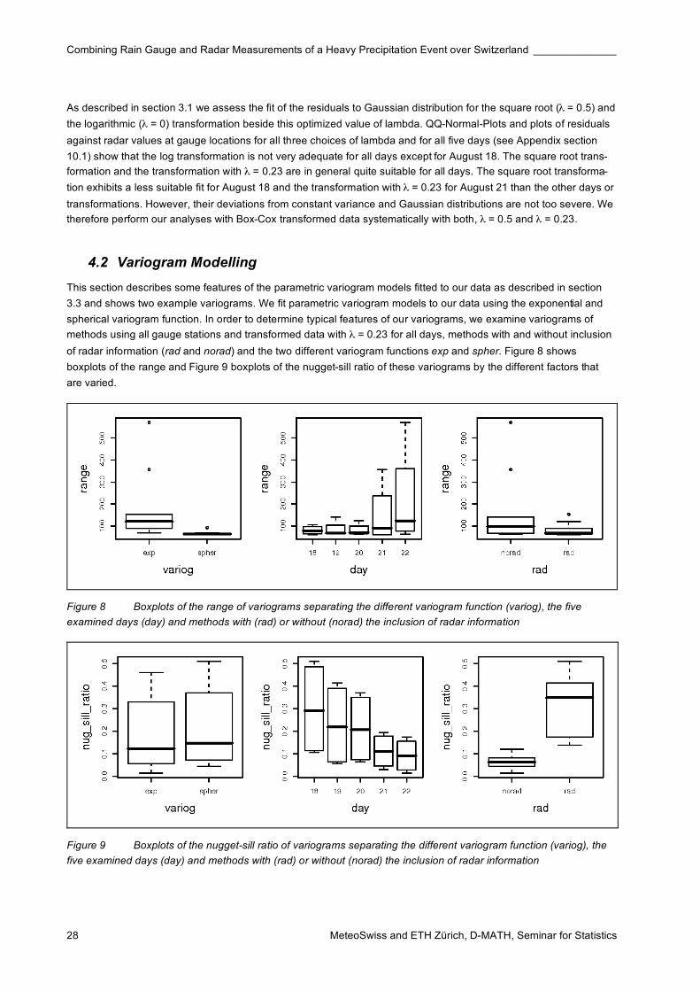
4.2 Variogram Modelling
This section describes some features of the parametric variogram models fitted to our data as described in section
3.3 and shows two example variograms. We fit parametric variogram models to our data using the exponential and
spherical variogram function. In order to determine typical features of our variograms, we examine variograms of
methods using all gauge stations and transformed data with " = 0.23 for all days, methods with and without inclusion
of radar information (rad and norad) and the two different variogram functions exp and spher. Figure 8 shows
boxplots of the range and Figure 9 boxplots of the nugget-sill ratio of these variograms by the different factors that
are varied.
Figure 8 Boxplots of the range of variograms separating the different variogram function (variog), the five
examined days (day) and methods with (rad) or without (norad) the inclusion of radar information
Figure 9 Boxplots of the nugget-sill ratio of variograms separating the different variogram function (variog), the
five examined days (day) and methods with (rad) or without (norad) the inclusion of radar information
_____________________________________________________________________________________ Results
Master Thesis | Rebekka Erdin | February 2009 29
The typical range of our variogram lies between about 60 and 130 km. A few outliers exhibit considerably larger
ranges. These exceptions are only found for exponential variogram functions and methods without the inclusion of
radar information. Figure 8 shows that the range of our variograms differs between the five observed days: August 18
to 20, with predominant convective precipitation character exhibit shorter ranges than August 21 and 22 with
stratiform precipitation patterns. This is what we expect by intuition and reflects the fact that convective precipitation
situations vary on smaller spatial scales than stratiform situations.
The typical nugget-sill ratio of our variograms is approximately 0.1. Figure 9 shows no major differences in nugget-sill
ratios for the two variogram functions, but a clearly different behaviour of methods with or without radar information:
norad models exhibit much smaller nugget-sill ratio than rad models. This can be explained by the fact that the sill is
reduced substantially by the introduction of radar information, as this information explains a part of the variance of the
phenomenon, whereas the nugget effect is not affected by this additional information. Stratiform precipitation
situations show a smaller nugget-sill ratio than convective precipitation situations, due to a larger sill and a smaller
nugget effect.
a)
b)
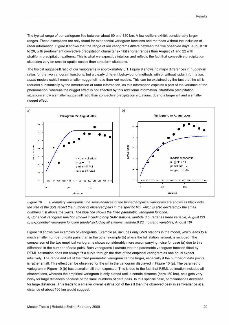
Figure 10 Exemplary variograms: the semivariances of the binned empirical variogram are shown as black dots,
the size of the dots reflect the number of observed pairs in the specific bin, which is also declared by the small
numbers just above the x-axis. The blue line shows the fitted parametric variogram function.
a) Spherical variogram function (model including only SMN stations, lambda 0.5, radar as trend variable, August 22)
b) Exponential variogram function (model including all stations, lambda 0.23, no trend variables, August 18)
Figure 10 shows two examples of variograms. Example (a) includes only SMN stations in the model, which leads to a
much smaller number of data pairs than in the other example (b) where the full station network is included. The
comparison of the two empirical variograms shows considerably more accompanying noise for case (a) due to this
difference in the number of data pairs. Both variograms illustrate that the parametric variogram function fitted by
REML estimation does not always fit a curve through the dots of the empirical variogram as one could expect
intuitively. The range and sill of the fitted parametric variogram can be larger, especially if the number of data points
is rather small. This effect can be observed for the sill in the variogram displayed in Figure 10 (a). The parametric
variogram in Figure 10 (b) has a smaller sill than expected. This is due to the fact that REML estimation includes all
observations, whereas the empirical variogram is only plotted until a certain distance (here 150 km), as it gets very
noisy for large distances because of the small numbers of data pairs. In this specific case, semivariances decrease
for large distances. This leads to a smaller overall estimation of the sill than the observed peak in semivariance at a
distance of about 100 km would suggest.

Combining Rain Gauge and Radar Measurements of a Heavy Precipitation Event over Switzerland ______________
30 MeteoSwiss and ETH Zürich, D-MATH, Seminar for Statistics
4.3 Analyses of Variance
As described in section 3.4.5, analyses of variance (ANOVA) are calculated for each of our five selected skill scores
(see section 3.4.4) as target variables. An overview on the different influencing factors is displayed in Table 3 (see
section 3.4.5). ANOVA models for each skill score and their results are presented in the following subsections. The
two skill scores rmse.sq and made.sq measure the same quality of a method, namely the general accuracy of
predictions. We will therefore describe the results for these two scores in one section. Selected model results will be
shown in the following, while more detailed R-Outputs and plots of residual analyses of the selected models can be
found in the Appendix (section 10.2).
For technical reasons (no convergence of the optimization algorithm performing MLE) it is not possible to include
more than one interaction of the random effect variable day with one of the fixed effect variables as additional
grouping variables at a time. Hence, for each skill score we test four possible models, including one of the four
possible interactions each. Models that show significant interactions of their grouping variables are further
considered. This was the case for only one or two of the four models for each skill score. In some cases, no
convergence was reached by the MLE algorithm for a model including one interaction. In this case we assess the
nature of the specific interaction by interaction plots. Results of the Likelihood-Ratio Tests and interaction plots
leading to the selection of models are listed in the Appendix (section 10.2). We will term p-values as significant or not
by comparing them to a significance level of 0.05, as customary in many statistical applications.
Plots for residual analyses of selected ANOVA models can be found in the Appendix (see section 10.2). They show
reasonable fulfilment of model assumptions in general, i.e. their residuals exhibit constant variance and
approximately Gaussian distribution.
Common to all models is the fact that variog, the variable distinguishing between the spherical and the exponential
variogram function, has no significant influence on the outcome of the skill scores. The interaction of variog with day
has no significant influence on any of the models either and is therefore not included in the selected models shown
below.
The influence of day as grouping variable, specifying the examined day and therefore the specific precipitation
situation, is significant for all skill scores. Hence, day is included in all models presented in the following subsections.
As day is a random effect, we are not interested in its coefficients, i. e. in a specific influence of one day, but only in
the part of remaining variance that is explained in general by it.
4.3.1 HK – the Ability to Distinguish between Dry and Wet
The skill score hk measures the ability of a method to distinguish between wet and dry areas. The dataset for the
ANOVA of hk consists therefore only of 96 observations, because hk cannot be defined for August 21, as there are
no dry stations on that day.
Figure 11 shows boxplots for hk as target variable, separating all values of hk by the categories of our five influencing
factors gauge network density (dens), different days examined (day), parameters for Box-Cox transformation of
gauge and radar data (lambda), inclusion of radar information (rad) and variogram function (variog). The last plot
shows the behaviour of hk of the three different categories of rad, namely no inclusion of radar (norad), inclusion of
radar by KED (rad) and inclusion of radar by OK of radar errors (raderr), for the dense (all) and less dense (smn)
gauge network.
The boxplots in Figure 11 show that the choice of transformation parameter lambda has a large influence on hk:
" = 0.23 yields much better results than " = 0.5. The inclusion of radar, especially by OK of radar errors, also
improves the value of hk. It can be seen that the choice of variogram function on the other hand does not influence
the result considerably. Furthermore we observe the surprising fact that the SMN network performs better in terms of
hk than the full gauge network. This is due to the interaction between dens:rad as can be seen in the interaction plot.
It shows that only for methods without radar information, hk increases as intuitively expected if all stations are
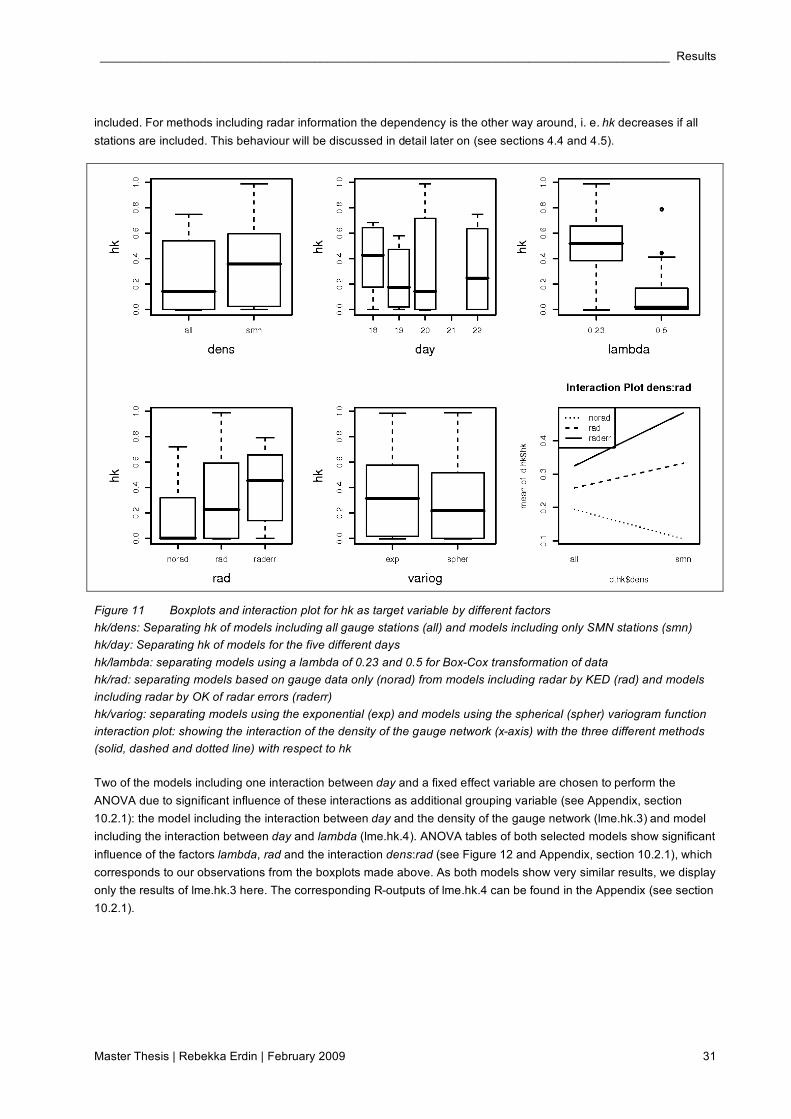
_____________________________________________________________________________________ Results
Master Thesis | Rebekka Erdin | February 2009 31
included. For methods including radar information the dependency is the other way around, i. e. hk decreases if all
stations are included. This behaviour will be discussed in detail later on (see sections 4.4 and 4.5).
Figure 11 Boxplots and interaction plot for hk as target variable by different factors
hk/dens: Separating hk of models including all gauge stations (all) and models including only SMN stations (smn)
hk/day: Separating hk of models for the five different days
hk/lambda: separating models using a lambda of 0.23 and 0.5 for Box-Cox transformation of data
hk/rad: separating models based on gauge data only (norad) from models including radar by KED (rad) and models
including radar by OK of radar errors (raderr)
hk/variog: separating models using the exponential (exp) and models using the spherical (spher) variogram function
interaction plot: showing the interaction of the density of the gauge network (x-axis) with the three different methods
(solid, dashed and dotted line) with respect to hk
Two of the models including one interaction between day and a fixed effect variable are chosen to perform the
ANOVA due to significant influence of these interactions as additional grouping variable (see Appendix, section
10.2.1): the model including the interaction between day and the density of the gauge network (lme.hk.3) and model
including the interaction between day and lambda (lme.hk.4). ANOVA tables of both selected models show significant
influence of the factors lambda, rad and the interaction dens:rad (see Figure 12 and Appendix, section 10.2.1), which
corresponds to our observations from the boxplots made above. As both models show very similar results, we display
only the results of lme.hk.3 here. The corresponding R-outputs of lme.hk.4 can be found in the Appendix (see section
10.2.1).
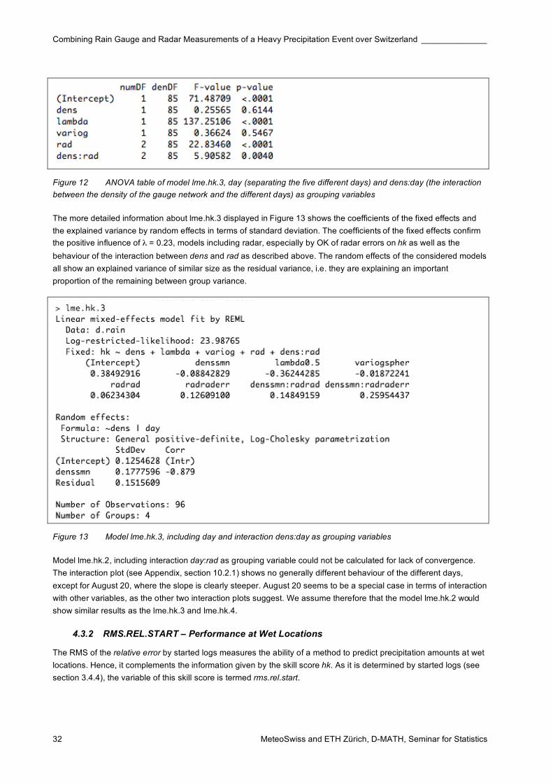
Combining Rain Gauge and Radar Measurements of a Heavy Precipitation Event over Switzerland ______________
32 MeteoSwiss and ETH Zürich, D-MATH, Seminar for Statistics
Figure 12 ANOVA table of model lme.hk.3, day (separating the five different days) and dens:day (the interaction
between the density of the gauge network and the different days) as grouping variables
The more detailed information about lme.hk.3 displayed in Figure 13 shows the coefficients of the fixed effects and
the explained variance by random effects in terms of standard deviation. The coefficients of the fixed effects confirm
the positive influence of " = 0.23, models including radar, especially by OK of radar errors on hk as well as the
behaviour of the interaction between dens and rad as described above. The random effects of the considered models
all show an explained variance of similar size as the residual variance, i.e. they are explaining an important
proportion of the remaining between group variance.
Figure 13 Model lme.hk.3, including day and interaction dens:day as grouping variables
Model lme.hk.2, including interaction day:rad as grouping variable could not be calculated for lack of convergence.
The interaction plot (see Appendix, section 10.2.1) shows no generally different behaviour of the different days,
except for August 20, where the slope is clearly steeper. August 20 seems to be a special case in terms of interaction
with other variables, as the other two interaction plots suggest. We assume therefore that the model lme.hk.2 would
show similar results as the lme.hk.3 and lme.hk.4.
4.3.2 RMS.REL.START – Performance at Wet Locations
The RMS of the relative error by started logs measures the ability of a method to predict precipitation amounts at wet
locations. Hence, it complements the information given by the skill score hk. As it is determined by started logs (see
section 3.4.4), the variable of this skill score is termed rms.rel.start.
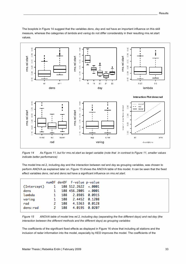
_____________________________________________________________________________________ Results
Master Thesis | Rebekka Erdin | February 2009 33
The boxplots in Figure 14 suggest that the variables dens, day and rad have an important influence on this skill
measure, whereas the categories of lambda and variog do not differ considerably in their resulting rms.rel.start
values.
Figure 14 As Figure 11, but for rms.rel.start as target variable (note that in contrast to Figure 11, smaller values
indicate better performance)
The model lme.rel.2, including day and the interaction between rad and day as grouping variables, was chosen to
perform ANOVA as explained later on. Figure 15 shows the ANOVA table of this model. It can be seen that the fixed
effect variables dens, rad and dens:rad have a significant influence on rms.rel.start.
Figure 15 ANOVA table of model lme.rel.2, including day (separating the five different days) and rad:day (the
interaction between the different methods and the different days) as grouping variables
The coefficients of the significant fixed effects as displayed in Figure 16 show that including all stations and the
inclusion of radar information into the model, especially by KED improves the model. The coefficients of the
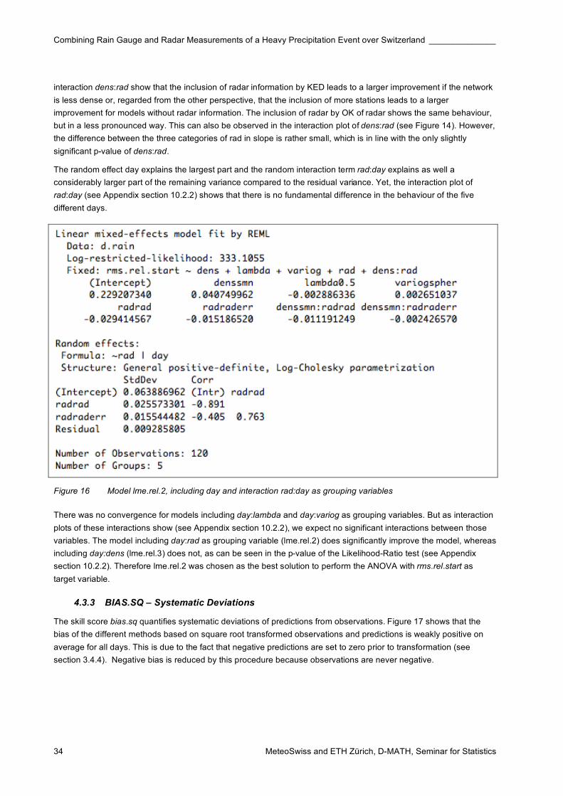
Combining Rain Gauge and Radar Measurements of a Heavy Precipitation Event over Switzerland ______________
34 MeteoSwiss and ETH Zürich, D-MATH, Seminar for Statistics
interaction dens:rad show that the inclusion of radar information by KED leads to a larger improvement if the network
is less dense or, regarded from the other perspective, that the inclusion of more stations leads to a larger
improvement for models without radar information. The inclusion of radar by OK of radar shows the same behaviour,
but in a less pronounced way. This can also be observed in the interaction plot of dens:rad (see Figure 14). However,
the difference between the three categories of rad in slope is rather small, which is in line with the only slightly
significant p-value of dens:rad.
The random effect day explains the largest part and the random interaction term rad:day explains as well a
considerably larger part of the remaining variance compared to the residual variance. Yet, the interaction plot of
rad:day (see Appendix section 10.2.2) shows that there is no fundamental difference in the behaviour of the five
different days.
Figure 16 Model lme.rel.2, including day and interaction rad:day as grouping variables
There was no convergence for models including day:lambda and day:variog as grouping variables. But as interaction
plots of these interactions show (see Appendix section 10.2.2), we expect no significant interactions between those
variables. The model including day:rad as grouping variable (lme.rel.2) does significantly improve the model, whereas
including day:dens (lme.rel.3) does not, as can be seen in the p-value of the Likelihood-Ratio test (see Appendix
section 10.2.2). Therefore lme.rel.2 was chosen as the best solution to perform the ANOVA with rms.rel.start as
target variable.
4.3.3 BIAS.SQ – Systematic Deviations
The skill score bias.sq quantifies systematic deviations of predictions from observations. Figure 17 shows that the
bias of the different methods based on square root transformed observations and predictions is weakly positive on
average for all days. This is due to the fact that negative predictions are set to zero prior to transformation (see
section 3.4.4). Negative bias is reduced by this procedure because observations are never negative.
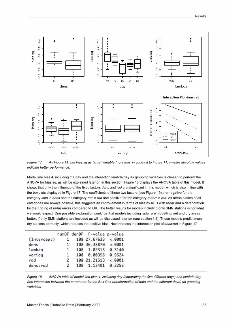
_____________________________________________________________________________________ Results
Master Thesis | Rebekka Erdin | February 2009 35
Figure 17 As Figure 11, but bias.sq as target variable (note that in contrast to Figure 11, smaller absolute values
indicate better performance)
Model lme.bias.4, including the day and the interaction lambda:day as grouping variables is chosen to perform the
ANOVA for bias.sq, as will be explained later on in this section. Figure 18 displays the ANOVA table of this model. It
shows that only the influence of the fixed factors dens and rad are significant in this model, which is also in line with
the boxplots displayed in Figure 17. The coefficients of these two factors (see Figure 19) are negative for the
category smn in dens and the category rad in rad and positive for the category raderr in rad. As mean biases of all
categories are always positive, this suggests an improvement in terms of bias by KED with radar and a deterioration
by the Kriging of radar errors compared to OK. The better results for models including only SMN stations is not what
we would expect. One possible explanation could be that models including radar are modelling wet and dry areas
better, if only SMN stations are included as will be discussed later on (see section 4.4). These models predict more
dry stations correctly, which reduces the positive bias. Nevertheless the interaction plot of dens:rad in Figure 17
Figure 18 ANOVA table of model lme.bias.4, including day (separating the five different days) and lambda:day
(the interaction between the parameter for the Box-Cox transformation of data and the different days) as grouping
variables

Combining Rain Gauge and Radar Measurements of a Heavy Precipitation Event over Switzerland ______________
36 MeteoSwiss and ETH Zürich, D-MATH, Seminar for Statistics
implies that also methods without radar information exhibit smaller biases if the SMN network only is included. We
suggest therefore that this behaviour is connected to a difference in characteristics between the SMN and the full
station network. This would mean that the SMN network is not a perfect random sample of the full gauge network.
The random effects day and lambda:day explain approximately equal parts of the remaining variance than the
residual variance. The interaction plot of lambda:day (see Appendix section 10.2.3) shows that August 18 behaves
very different from all other days: its bias is considerably larger for the transformation with a lambda of 0.5 than with a
lambda of 0.23, while the biases are of similar scale for both lambdas for the other four days. This behaviour of
August 18 is responsible for the difference between the two lambdas in terms of bias as observed in the correspon-
ding boxplot in Figure 17. We suggest the fact that the square root transformation does not suite the data of August
18 very well (as described in section 4.1) as a possible reason for this observed difference between the five days.
Figure 19 Model lme.bias.4, including day and interaction lambda:day as grouping variables
Models lme.bias.3 and lme.bias.5 including dens:day and variog:day respectively as additional grouping variable do
not significantly improve the model, but model lme.bias.4 including lambda:day does (see Appendix section 10.2.3).
The model lme.bias.2 including the interaction term rad:day as grouping variable does not reach convergence. The
interaction plot of rad:day (see Appendix section 10.2.3) shows that there would possibly be a significant
improvement of the model by this grouping term. It can be seen that August 20 and to a smaller extent also August
22 show a different behaviour. Their bias is smaller for methods including radar by the Kriging of radar errors, than for
methods without the inclusion of radar information, while it is the other way around for the other three examined days.
Common to all days is that the smallest bias is achieved by methods including radar information by KED.
4.3.4 RMSE.SQ and MADE.SQ – Overall Performance
This subsection describes the results of ANOVA with rmse.sq and made.sq as target variables. These two skill
scores describe the general accuracy of prediction of a model, i. e. in contrast to rms.rel.start, they consider
predictions at wet and dry stations. RMSE is a widely known and used measure, but with the weakness of being
sensitive to outliers, whereas its robust equivalent MADE is less known. The results of the ANOVA of the two skill
scores are very similar. We therefore primarily present the results of rmse.sq in this section and mention the results
of made.sq only in terms of differences to these results. Plots and R-outputs of the ANOVA with made.sq as target
variables can be found in the Appendix (section 10.2.5).

_____________________________________________________________________________________ Results
Master Thesis | Rebekka Erdin | February 2009 37
Figure 20 As Figure 11, but for rmse.sq as target variable (note that in contrast to Figure 11, smaller values
indicate better performance)
There are two models selected to perform the ANOVA for rmse.sq (lme.rmse.2 and lme.rmse.3) and one to perform
the ANOVA for made.sq (lme.made.4) as will be described at the end of this section. As they show all very similar
results, we will present only lme.rmse.2, the model for rmse.sq including day and the interaction rad:day as grouping
variables, in detail here. Outputs of the two other models can be found in the Appendix (section 10.2.4 and 10.2.5).
The boxplots displayed in Figure 20 suggest that dens, day, rad and the interaction dens:rad influence rmse.sq
considerably and the corresponding F-Tests of the ANOVA presented in Figure 21 confirm this impression. The
influence of lambda is also significant but less articulately.
Figure 21 ANOVA table of model lme.rmse.2, including day (separating the five different days) and rad:day (the
interaction between the different methods and the different days) as grouping variables
The coefficients in Figure 22 show that a denser gauge network, a lambda of 0.23 and the inclusion of radar
information, especially by KED have a positive, i.e. decreasing, influence on rmse.sq. The coefficients of the
interaction term dens:rad are negative for the combination of the SMN network with the inclusion of radar. This
means that a denser network is more important for models without radar, or the other way around, that the
information of radar is more important if the gauge network is less dense. The interaction plot of dens:rad (Figure 20)
illustrates this behaviour.
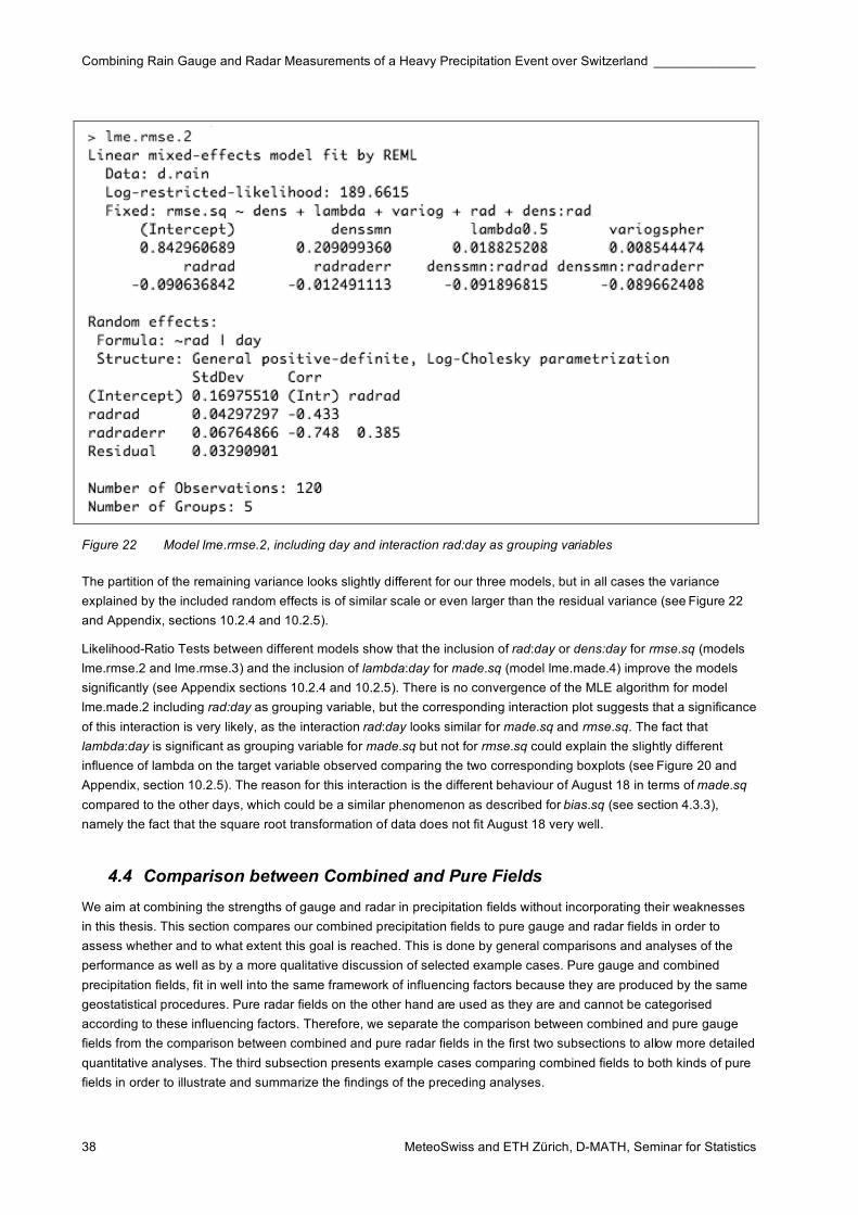
Combining Rain Gauge and Radar Measurements of a Heavy Precipitation Event over Switzerland ______________
38 MeteoSwiss and ETH Zürich, D-MATH, Seminar for Statistics
Figure 22 Model lme.rmse.2, including day and interaction rad:day as grouping variables
The partition of the remaining variance looks slightly different for our three models, but in all cases the variance
explained by the included random effects is of similar scale or even larger than the residual variance (see Figure 22
and Appendix, sections 10.2.4 and 10.2.5).
Likelihood-Ratio Tests between different models show that the inclusion of rad:day or dens:day for rmse.sq (models
lme.rmse.2 and lme.rmse.3) and the inclusion of lambda:day for made.sq (model lme.made.4) improve the models
significantly (see Appendix sections 10.2.4 and 10.2.5). There is no convergence of the MLE algorithm for model
lme.made.2 including rad:day as grouping variable, but the corresponding interaction plot suggests that a significance
of this interaction is very likely, as the interaction rad:day looks similar for made.sq and rmse.sq. The fact that
lambda:day is significant as grouping variable for made.sq but not for rmse.sq could explain the slightly different
influence of lambda on the target variable observed comparing the two corresponding boxplots (see Figure 20 and
Appendix, section 10.2.5). The reason for this interaction is the different behaviour of August 18 in terms of made.sq
compared to the other days, which could be a similar phenomenon as described for bias.sq (see section 4.3.3),
namely the fact that the square root transformation of data does not fit August 18 very well.
4.4 Comparison between Combined and Pure Fields
We aim at combining the strengths of gauge and radar in precipitation fields without incorporating their weaknesses
in this thesis. This section compares our combined precipitation fields to pure gauge and radar fields in order to
assess whether and to what extent this goal is reached. This is done by general comparisons and analyses of the
performance as well as by a more qualitative discussion of selected example cases. Pure gauge and combined
precipitation fields, fit in well into the same framework of influencing factors because they are produced by the same
geostatistical procedures. Pure radar fields on the other hand are used as they are and cannot be categorised
according to these influencing factors. Therefore, we separate the comparison between combined and pure gauge
fields from the comparison between combined and pure radar fields in the first two subsections to allow more detailed
quantitative analyses. The third subsection presents example cases comparing combined fields to both kinds of pure
fields in order to illustrate and summarize the findings of the preceding analyses.
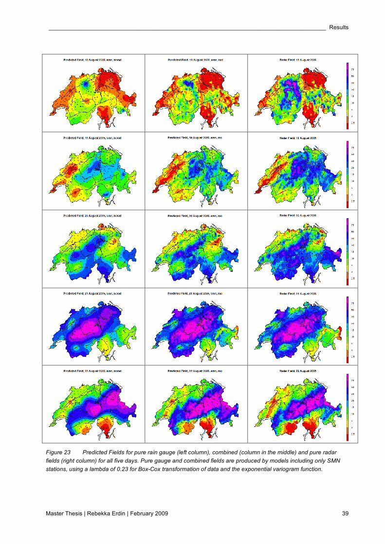
_____________________________________________________________________________________ Results
Master Thesis | Rebekka Erdin | February 2009 39
Figure 23 Predicted Fields for pure rain gauge (left column), combined (column in the middle) and pure radar
fields (right column) for all five days. Pure gauge and combined fields are produced by models including only SMN
stations, using a lambda of 0.23 for Box-Cox transformation of data and the exponential variogram function.
Combining Rain Gauge and Radar Measurements of a Heavy Precipitation Event over Switzerland ______________
40 MeteoSwiss and ETH Zürich, D-MATH, Seminar for Statistics
Section 4.3 has shown that the Box-Cox transformation using a lambda of 0.23 shows better results in general and
that the choice of variogram function has no influence on performance. The exponential variogram function fits the
data reasonably well for the chosen example cases (see Appendix, section 10.3.3 and 10.3.4). We therefore choose
" = 0.23 and the exponential variogram function for all our example cases in this section. Many examples are using
models based on the less dense gauge network, using only SMN stations. We focus on this case for two reasons:
First, this case offers the possibility of applying the same methods for shorter time scales, because of the time
resolution of SMN stations of 10 minutes. Second, the added value of combining gauge and radar is larger and
therefore better visible in this situation (see section 4.3). Nevertheless, we present also examples using the full gauge
network in order to assess the best available precipitation fields.
Figure 23 gives an overview of combined and pure fields for all five days. It shows the differences in precipitation
patterns between the days as described in section 2.2 - namely variations of precipitation fields on smaller scale
because of predominantly convective precipitation for August 18 and 19, smooth patterns because of stratiform
precipitation for August 21 and 22 and a situation in between those two groups for August 20. Many typical
differences between the three kinds of fields that will be discussed in more detail later on can already be observed in
the comparison of these fields. First of all, there is a striking difference in smoothness between pure gauge fields and
fields including radar. Second it shows the radar bias - positive for the first three and negative for the latter two days -
and its removal in combined fields. The general incorporation of radar pattern into combined fields, as well as the
mitigating influence of gauges on it in some regions, can also be observed.
4.4.1 Combined versus Pure Gauge Fields
This subsection discusses differences between models based on gauge information only and models including radar
information additionally. This is done on the one hand by a closer look at the quantitative results of the systematic
evaluation of different models, on the other hand by the qualitative analysis of one example case.
As we have seen in section 4.3, the quantitative analysis shows a general improvement of prediction if radar is
included additionally into models. Figure 24 shows boxplots for the five different skill scores, separating methods with
(categories rad and raderr of factor rad) and without (category norad) radar information in order to get a better
overview of the added value of radar information. It can be seen that including radar improves all skill scores, except
for bias.sq. The improvement is largest for hk, where typical values without radar are between 0 and 0.3, whereas
methods including radar reach values between 0.05 and 0.65. The medians of bias.sq are fairly comparable, but the
spread of methods including radar is larger. This is due to the fact that methods including radar by Kriging of radar
errors exhibit larger, and methods including radar by KED smaller biases than methods without radar (see section
4.3.3).
After this general comparison, we would like to look at the added value by the inclusion of radar information in more
detail. Are there situations where the improvement by radar is especially large? We have seen, that the interaction
term dens:rad is significant for all skill scores, except for bias.sq (see section 4.3). The coefficients of all these
significant interactions indicate that radar information improves the model stronger if the included network is less
dense. This behaviour is what we would expect intuitively, as the lack of information about the spatial pattern
between stations increases in a less dense network and the additional information about this pattern has therefore a
larger value.
The skill score hk exhibits a strange behaviour in its interaction between network density and the variable rad : the
results for models including radar are better if only SMN stations are included in the model than if all stations are
included. This is counter-intuitive, because one expects that including additional information about a phenomenon
improves the model. We suppose the fact that radar is a very good predictor of rain occurrence as discussed later on
(see section 4.4.2, especially Figure 28) as reason for this strange interaction pattern: Additional stations included in
the model overlap and soften the more accurate radar information about wet and dry areas locally. This deteriorates
the result in terms of hk.
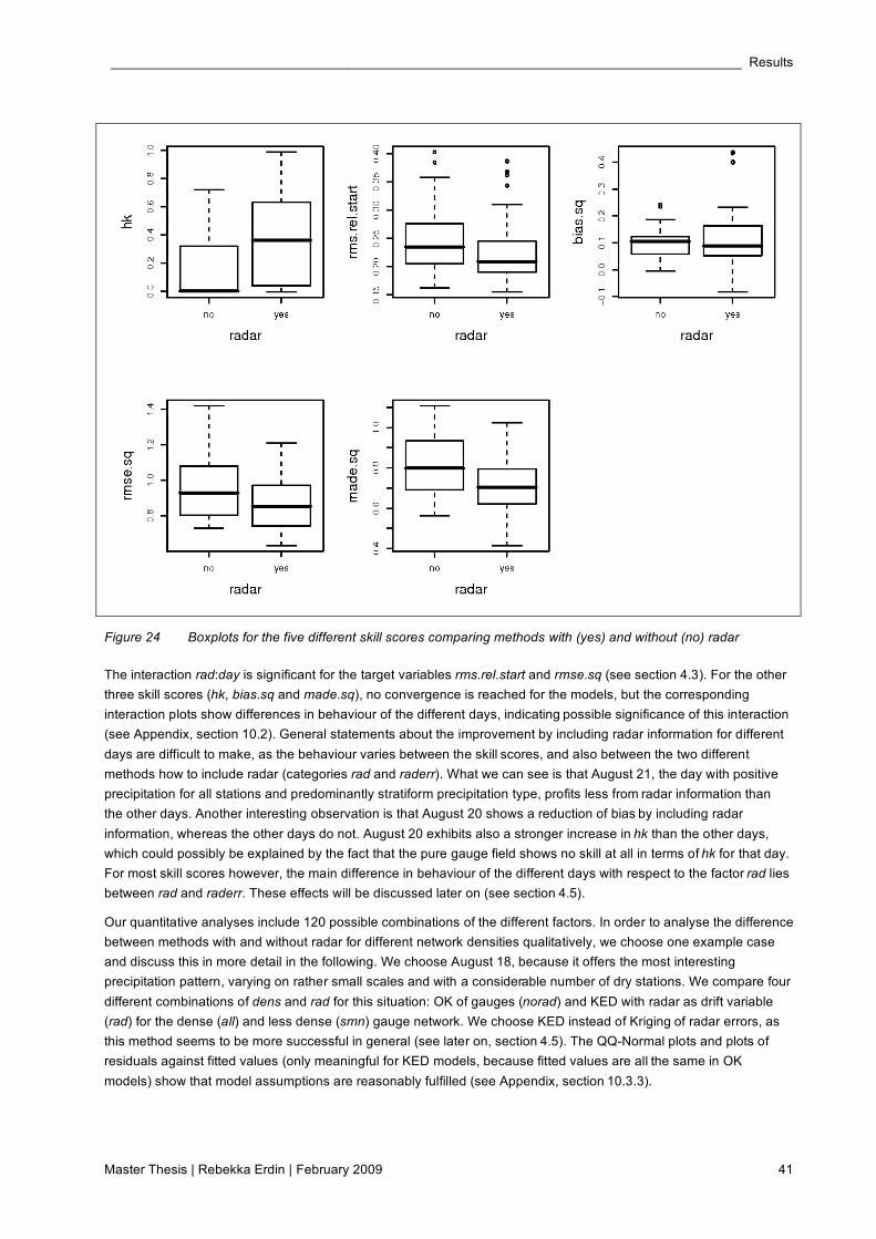
_____________________________________________________________________________________ Results
Master Thesis | Rebekka Erdin | February 2009 41
Figure 24 Boxplots for the five different skill scores comparing methods with (yes) and without (no) radar
The interaction rad:day is significant for the target variables rms.rel.start and rmse.sq (see section 4.3). For the other
three skill scores (hk, bias.sq and made.sq), no convergence is reached for the models, but the corresponding
interaction plots show differences in behaviour of the different days, indicating possible significance of this interaction
(see Appendix, section 10.2). General statements about the improvement by including radar information for different
days are difficult to make, as the behaviour varies between the skill scores, and also between the two different
methods how to include radar (categories rad and raderr). What we can see is that August 21, the day with positive
precipitation for all stations and predominantly stratiform precipitation type, profits less from radar information than
the other days. Another interesting observation is that August 20 shows a reduction of bias by including radar
information, whereas the other days do not. August 20 exhibits also a stronger increase in hk than the other days,
which could possibly be explained by the fact that the pure gauge field shows no skill at all in terms of hk for that day.
For most skill scores however, the main difference in behaviour of the different days with respect to the factor rad lies
between rad and raderr. These effects will be discussed later on (see section 4.5).
Our quantitative analyses include 120 possible combinations of the different factors. In order to analyse the difference
between methods with and without radar for different network densities qualitatively, we choose one example case
and discuss this in more detail in the following. We choose August 18, because it offers the most interesting
precipitation pattern, varying on rather small scales and with a considerable number of dry stations. We compare four
different combinations of dens and rad for this situation: OK of gauges (norad) and KED with radar as drift variable
(rad) for the dense (all) and less dense (smn) gauge network. We choose KED instead of Kriging of radar errors, as
this method seems to be more successful in general (see later on, section 4.5). The QQ-Normal plots and plots of
residuals against fitted values (only meaningful for KED models, because fitted values are all the same in OK
models) show that model assumptions are reasonably fulfilled (see Appendix, section 10.3.3).

Combining Rain Gauge and Radar Measurements of a Heavy Precipitation Event over Switzerland ______________
42 MeteoSwiss and ETH Zürich, D-MATH, Seminar for Statistics
Table 4 lists the skill scores of the four methods examined. Also for this exemplary case, we can observe an
improvement of skill scores by the inclusion of radar as well as by the inclusion of a denser network. The generally
observed fact that methods including radar exhibit a higher hk for the SMN network does not apply to this specific
situation, but the value of hk is of similar size for the two methods including radar, whereas there is a considerable
improvement by including more stations (by a factor 1.7) for the pure gauge method. We observe a larger
improvement of all skill scores by including radar in the less dense network (smn) in our example, as this was the
case for the average of all combinations. The overall skill measure rmse.sq for example decreases by 22% by
including radar for the SMN network, but only by 18% for the full station network. The situation for its robust
counterpart made.sq is even more pronounced with a decrease of 40% for the SMN network in contrast to a
decrease of 20% for the full network.
This example comparing four situations as listed in Table 4 leads also to another interesting question: if we consider
the precipitation field based on the SMN gauge network only as basis – does the additional information of radar or
that of 365 gauge measurements (all other stations than SMN) improve the predicted precipitation field stronger?
This corresponds to a comparison between the first method, including the full station network but no radar (dens:all,
rad:norad), and the last method, including the less dense network and radar(dens:smn, rad:rad). We observe that the
radar adds more value in terms of all five skill scores in this particular case. Nevertheless, we would like to point out
that this result could be influenced by the large number of stations in flatland regions compared to a relatively small
number of stations in mountainous regions. Our skill scores are based on predictions at station locations, and
therefore influenced strongly by the performance over flatland. As radar measurements are afflicted by larger
uncertainties in mountainous terrain (see sections 2.1.2 and 3.3.4), this could favour methods including radar.
Boxplots of this comparison for all systematically evaluated situations of the full station network without radar versus
the SMN network including radar by KED or by OK of radar errors as well as plots of their interaction with day can be
found in the Appendix (see section 10.3.1). It can be seen that the better performance of radar can only be
generalized for all days and situations in terms of hk. For the other skill scores, including radar by KED adds
approximately the same value as including the 365 additional gauges. Including radar by OK of radar errors on the
other hand, exhibits inferior results than the other two methods. The fact that August 18 profits more strongly from
radar information compared to gauge information than the other four days is not very surprising, as this day exhibits
the strongest small-scale variations in precipitation pattern because of predominantly convective precipitation.
Table 4 Skill scores of exemplary methods of August, 18, using a lambda of 0.23 for Box-Cox transformation of
data and the exponential variogram function - comparing methods with (rad) and without (norad) radar as a trend
variable including the full (all) and the SMN (smn) gauge network
dens rad hk rms.rel.start bias.sq rmse.sq made.sq
all norad 0.52 0.35 0.124 0.79 0.56
all rad 0.64 0.28 0.094 0.65 0.45
smn norad 0.30 0.39 0.063 0.92 0.78
smn rad 0.61 0.31 0.092 0.72 0.47
The observations based on the comparison of skill scores are confirmed if we look at the scatterplots of predictions
against observations in Figure 25. In addition, these scatterplots show that models based on gauge information only
exhibit particular difficulties in modelling the largest precipitation amounts of the situation, whereas models including
radar are capturing these large observations better in this example.

_____________________________________________________________________________________ Results
Master Thesis | Rebekka Erdin | February 2009 43
Figure 25 Scatterplots of predictions and observations comparing methods with (to the right: rad) and without (to
the left: norad) radar as a trend variable including the full (top, all) and the SMN (bottom, smn) gauge network for
August 18, using a lambda of 0.23 for Box-Cox transformation of data and the exponential variogram function
Figure 26 shows the predicted precipitation fields by the four different methods for August 18. The comparison
between models without (on the right hand side) and models with (on the left hand side) radar information illustrates a
different structure of the precipitation patterns: models without radar exhibit much smoother predicted fields,
especially for the SMN network. It is intuitively obvious that precipitation patterns varying on smaller scales and of
irregular shape, as produced by models including radar, are more likely to reflect real precipitation. Another
qualitative effect that we can observe looking at the two fields at the bottom is that the influence of one SMN station
included in the model (black dots) can be spatially extended or mitigated by the inclusion of radar, depending on the
radar pattern (e.g. the influence of the station at Interlaken is mitigated and the influence of the station at Wynau is
extended). This ability of the combined model by KED seems useful, as we expect stations to be more or less
representative of their surrounding, depending on the topography and precipitation situation.
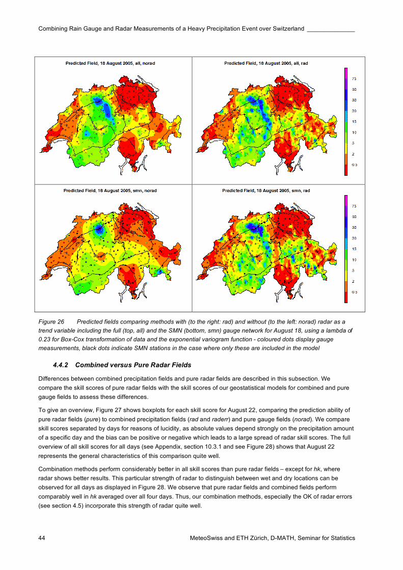
Combining Rain Gauge and Radar Measurements of a Heavy Precipitation Event over Switzerland ______________
44 MeteoSwiss and ETH Zürich, D-MATH, Seminar for Statistics
Figure 26 Predicted fields comparing methods with (to the right: rad) and without (to the left: norad) radar as a
trend variable including the full (top, all) and the SMN (bottom, smn) gauge network for August 18, using a lambda of
0.23 for Box-Cox transformation of data and the exponential variogram function - coloured dots display gauge
measurements, black dots indicate SMN stations in the case where only these are included in the model
4.4.2 Combined versus Pure Radar Fields
Differences between combined precipitation fields and pure radar fields are described in this subsection. We
compare the skill scores of pure radar fields with the skill scores of our geostatistical models for combined and pure
gauge fields to assess these differences.
To give an overview, Figure 27 shows boxplots for each skill score for August 22, comparing the prediction ability of
pure radar fields (pure) to combined precipitation fields (rad and raderr) and pure gauge fields (norad). We compare
skill scores separated by days for reasons of lucidity, as absolute values depend strongly on the precipitation amount
of a specific day and the bias can be positive or negative which leads to a large spread of radar skill scores. The full
overview of all skill scores for all days (see Appendix, section 10.3.1 and see Figure 28) shows that August 22
represents the general characteristics of this comparison quite well.
Combination methods perform considerably better in all skill scores than pure radar fields – except for hk, where
radar shows better results. This particular strength of radar to distinguish between wet and dry locations can be
observed for all days as displayed in Figure 28. We observe that pure radar fields and combined fields perform
comparably well in hk averaged over all four days. Thus, our combination methods, especially the OK of radar errors
(see section 4.5) incorporate this strength of radar quite well.
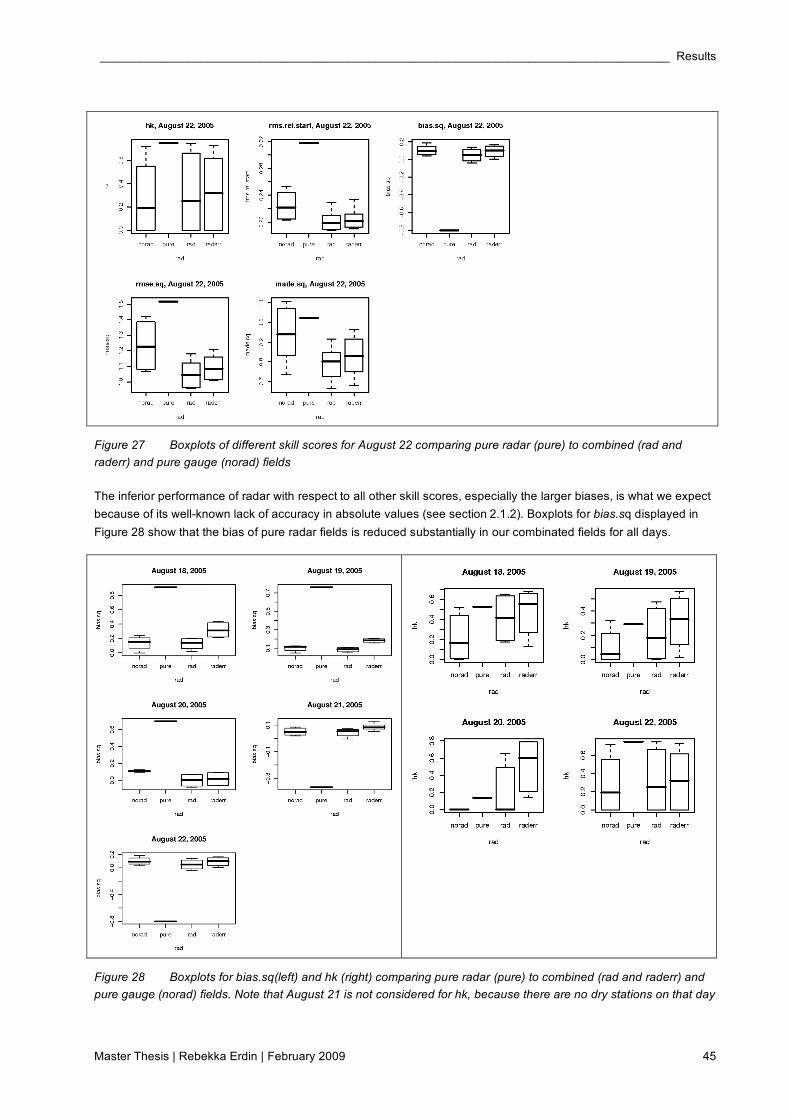
_____________________________________________________________________________________ Results
Master Thesis | Rebekka Erdin | February 2009 45
Figure 27 Boxplots of different skill scores for August 22 comparing pure radar (pure) to combined (rad and
raderr) and pure gauge (norad) fields
The inferior performance of radar with respect to all other skill scores, especially the larger biases, is what we expect
because of its well-known lack of accuracy in absolute values (see section 2.1.2). Boxplots for bias.sq displayed in
Figure 28 show that the bias of pure radar fields is reduced substantially in our combinated fields for all days.
Figure 28 Boxplots for bias.sq(left) and hk (right) comparing pure radar (pure) to combined (rad and raderr) and
pure gauge (norad) fields. Note that August 21 is not considered for hk, because there are no dry stations on that day
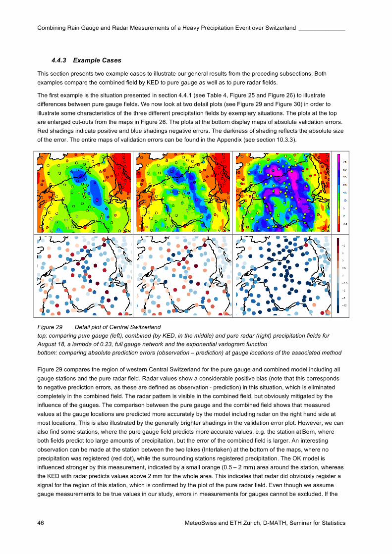
Combining Rain Gauge and Radar Measurements of a Heavy Precipitation Event over Switzerland ______________
46 MeteoSwiss and ETH Zürich, D-MATH, Seminar for Statistics
4.4.3 Example Cases
This section presents two example cases to illustrate our general results from the preceding subsections. Both
examples compare the combined field by KED to pure gauge as well as to pure radar fields.
The first example is the situation presented in section 4.4.1 (see Table 4, Figure 25 and Figure 26) to illustrate
differences between pure gauge fields. We now look at two detail plots (see Figure 29 and Figure 30) in order to
illustrate some characteristics of the three different precipitation fields by exemplary situations. The plots at the top
are enlarged cut-outs from the maps in Figure 26. The plots at the bottom display maps of absolute validation errors.
Red shadings indicate positive and blue shadings negative errors. The darkness of shading reflects the absolute size
of the error. The entire maps of validation errors can be found in the Appendix (see section 10.3.3).
Figure 29 Detail plot of Central Switzerland
top: comparing pure gauge (left), combined (by KED, in the middle) and pure radar (right) precipitation fields for
August 18, a lambda of 0.23, full gauge network and the exponential variogram function
bottom: comparing absolute prediction errors (observation – prediction) at gauge locations of the associated method
Figure 29 compares the region of western Central Switzerland for the pure gauge and combined model including all
gauge stations and the pure radar field. Radar values show a considerable positive bias (note that this corresponds
to negative prediction errors, as these are defined as observation - prediction) in this situation, which is eliminated
completely in the combined field. The radar pattern is visible in the combined field, but obviously mitigated by the
influence of the gauges. The comparison between the pure gauge and the combined field shows that measured
values at the gauge locations are predicted more accurately by the model including radar on the right hand side at
most locations. This is also illustrated by the generally brighter shadings in the validation error plot. However, we can
also find some stations, where the pure gauge field predicts more accurate values, e.g. the station at Bern, where
both fields predict too large amounts of precipitation, but the error of the combined field is larger. An interesting
observation can be made at the station between the two lakes (Interlaken) at the bottom of the maps, where no
precipitation was registered (red dot), while the surrounding stations registered precipitation. The OK model is
influenced stronger by this measurement, indicated by a small orange (0.5 – 2 mm) area around the station, whereas
the KED with radar predicts values above 2 mm for the whole area. This indicates that radar did obviously register a
signal for the region of this station, which is confirmed by the plot of the pure radar field. Even though we assume
gauge measurements to be true values in our study, errors in measurements for gauges cannot be excluded. If the
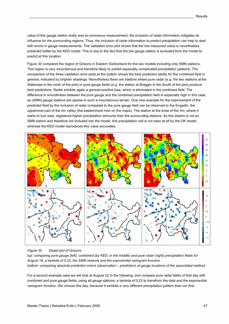
_____________________________________________________________________________________ Results
Master Thesis | Rebekka Erdin | February 2009 47
value of this gauge station really was an erroneous measurement, the inclusion of radar information mitigates its
influence for the surrounding regions. Thus, the inclusion of radar information to predict precipitation can help to deal
with errors in gauge measurements. The validation error plot shows that the low measured value is nevertheless
predicted better by the KED model. This is due to the fact that the low gauge station is excluded from the model to
predict at this location.
Figure 30 compares the region of Grisons in Eastern Switzerland for the two models including only SMN stations.
This region is very mountainous and therefore likely to exhibit especially complicated precipitation patterns. The
comparison of the three validation error plots at the bottom shows the best prediction ability for the combined field in
general, indicated by brighter shadings. Nevertheless there are stations where pure radar (e.g. the two stations at the
Walensee in the north of the plot) or pure gauge fields (e.g. the station at Braggio in the South of the plot) produce
best predictions. Radar exhibits again a general positive bias, which is eliminated in the combined field. The
difference in smoothness between the pure gauge and the combined precipitation field is especially high in this case,
as (SMN) gauge stations are sparse in such a mountainous terrain. One nice example for the improvement of the
predicted field by the inclusion of radar compared to the pure gauge field can be observed in the Engadin, the
uppermost part of the Inn valley (the easternmost river on the maps). The station at the knee of the Inn, where it
starts to turn east, registered higher precipitation amounts than the surrounding stations. As this station is not an
SMN station and therefore not included into the model, this precipitation cell is not seen at all by the OK model,
whereas the KED model reproduces this value accurately.
Figure 30 Detail plot of Grisons
top: comparing pure gauge (left), combined (by KED, in the middle) and pure radar (right) precipitation fields for
August 18, a lambda of 0.23, the SMN network and the exponential variogram function
bottom: comparing absolute prediction errors (observation – prediction) at gauge locations of the associated method
For a second example case we will look at August 22 in the following, and compare pure radar fields of that day with
combined and pure gauge fields, using all gauge stations, a lambda of 0.23 to transform the data and the exponential
variogram function. We choose this day, because it exhibits a very different precipitation pattern than our first
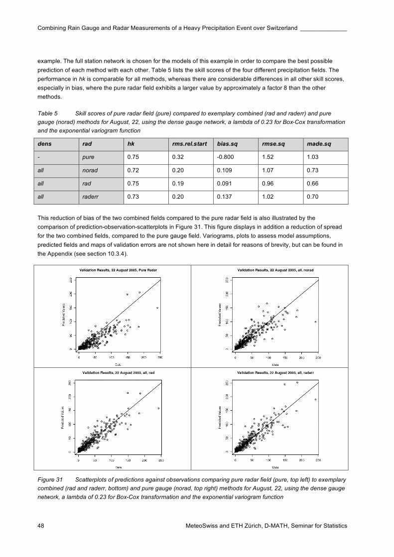
Combining Rain Gauge and Radar Measurements of a Heavy Precipitation Event over Switzerland ______________
48 MeteoSwiss and ETH Zürich, D-MATH, Seminar for Statistics
example. The full station network is chosen for the models of this example in order to compare the best possible
prediction of each method with each other. Table 5 lists the skill scores of the four different precipitation fields. The
performance in hk is comparable for all methods, whereas there are considerable differences in all other skill scores,
especially in bias, where the pure radar field exhibits a larger value by approximately a factor 8 than the other
methods.
Table 5 Skill scores of pure radar field (pure) compared to exemplary combined (rad and raderr) and pure
gauge (norad) methods for August, 22, using the dense gauge network, a lambda of 0.23 for Box-Cox transformation
and the exponential variogram function
dens rad hk rms.rel.start bias.sq rmse.sq made.sq
- pure 0.75 0.32 -0.800 1.52 1.03
all norad 0.72 0.20 0.109 1.07 0.73
all rad 0.75 0.19 0.091 0.96 0.66
all raderr 0.73 0.20 0.137 1.02 0.70
This reduction of bias of the two combined fields compared to the pure radar field is also illustrated by the
comparison of prediction-observation-scatterplots in Figure 31. This figure displays in addition a reduction of spread
for the two combined fields, compared to the pure gauge field. Variograms, plots to assess model assumptions,
predicted fields and maps of validation errors are not shown here in detail for reasons of brevity, but can be found in
the Appendix (see section 10.3.4).
Figure 31 Scatterplots of predictions against observations comparing pure radar field (pure, top left) to exemplary
combined (rad and raderr, bottom) and pure gauge (norad, top right) methods for August, 22, using the dense gauge
network, a lambda of 0.23 for Box-Cox transformation and the exponential variogram function

_____________________________________________________________________________________ Results
Master Thesis | Rebekka Erdin | February 2009 49
Summing up, our two examples shows a successful combination of the strengths of rain gauge and radar
measurements without the incorporation of their weaknesses in our combined precipitation fields. The improvement
of results by combined fields is particularly evident if models including only SMN stations are considered. As results
in this and the preceding sections (see section 4.3, 4.4.1 and 4.4.2) show, we may generalize this conclusion for all
observed days and methods,.
4.5 Comparison of Combination Methods
We have applied two different geostatistical methods to include radar information, KED with radar as trend variable
(see section 3.3.2) and OK of radar errors (see section 3.3.1). This subsection discusses characteristics of these two
approaches and differences between them.
Figure 32 shows boxplots of the five different skill scores of all systematically evaluated methods including radar
information, separating categories rad (KED with radar) and raderr (OK of radar errors). KED exhibits better results
on average for all skill scores, except for hk, where the Kriging of radar errors shows better values. The advantage of
KED seems especially large in terms of bias.sq. Corresponding ANOVA (see Appendix, section 10.4), stratifying
results additionally by different days (day), network densities (dens), and Box-Cox parameters (lambda), show clearly
significant p-values for all these observed differences between the two methods.
Figure 32 Boxplots for five different skill scores comparing methods including radar by KED (rad) and by OK of
radar errors (raderr)
We expect KED to offer more flexibility in the inclusion of radar, because radar information is included by multiplying
it by a specifically estimated coefficient (() and the model includes an additional constant (') in the trend (see section
3.3.2). The OK of radar errors on the other hand includes radar information as it is, i. e. ( always equals one and
allows only an additional constant '. This implies that errors in the variance of radar measurements cannot be
alleviated by OK of radar errors.

Combining Rain Gauge and Radar Measurements of a Heavy Precipitation Event over Switzerland ______________
50 MeteoSwiss and ETH Zürich, D-MATH, Seminar for Statistics
We are therefore interested in the size of the coefficient (, of our KED models. We observe that ( is always between
zero and one and most models show values of about 0.7 to 0.8. The constant ' compensates for the lack of
precipitation amount that is generated by including radar by a factor smaller than one (as radar is calibrated to the
event and therefore unbiased in average values). In summary, the radar pattern is included in a softened version in
our KED models compared to the Kriging of radar errors.
The better results in hk by Kriging of radar errors can thus again be explained by the fact that radar is better in
distinguishing between wet and dry areas than kriged gauges. As Kriging of radar errors follows the radar pattern to a
higher extent than KED, it takes better advantage of this strength of radar information.
The better results of KED with respect to all other skill scores can be explained by the higher flexibility of the model to
adapt to a specific situation, by estimating an additional parameter.
Table 6 Skill scores of exemplary situation comparing KED with radar (rad) and OK of radar errors (raderr) for
August, 20, using the full gauge network, a lambda of 0.23 for Box-Cox transformation and the exponential variogram
function
dens rad hk rms.rel.start bias.sq rmse.sq made.sq
all rad 0.00 0.17 0.065 0.63 0.59
all raderr 0.42 0.18 0.091 0.68 0.60
To illustrate the differences between the two methods, we look at an example case in more detail. We choose August
20, the dense gauge network including all stations, Box-Cox transformation with "=0.23 and the exponential
variogram function as example and compare the results of OK of radar errors for this situation with those of KED with
radar. August 20 is chosen, because the difference in hk - one of the results of the general comparison that we are
especially interested in - is particularly high for that day. The skill scores listed in Table 6 show that this case is
representative for the general characteristics of the two methods: OK of radar errors yields better results in terms of
hk, whereas KED with radar yields better results in terms of all other skill scores. Figure 33 shows scatterplots of the
cross-validated predictions against the observed values at stations for both methods. KED with radar shows a slightly
smaller especially for too large predictions, which could explain the reduction of positive bias.
Figure 33 Scatterplots of predictions against observations of exemplary situation comparing KED with radar (rad,
left) and OK of radar errors (raderr, right) for August, 20, using the full gauge network, a lambda of 0.23 for Box-Cox
transformation and the exponential variogram function
Predicted fields of the two methods are displayed in Figure 34. As the difference between these two fields is hard to
detect on this scale, plot (c) shows the field of differences between them (prediction by OK of radar error – Prediction
of KED with radar). We observe largest absolute differences between the two fields for regions, where the radar
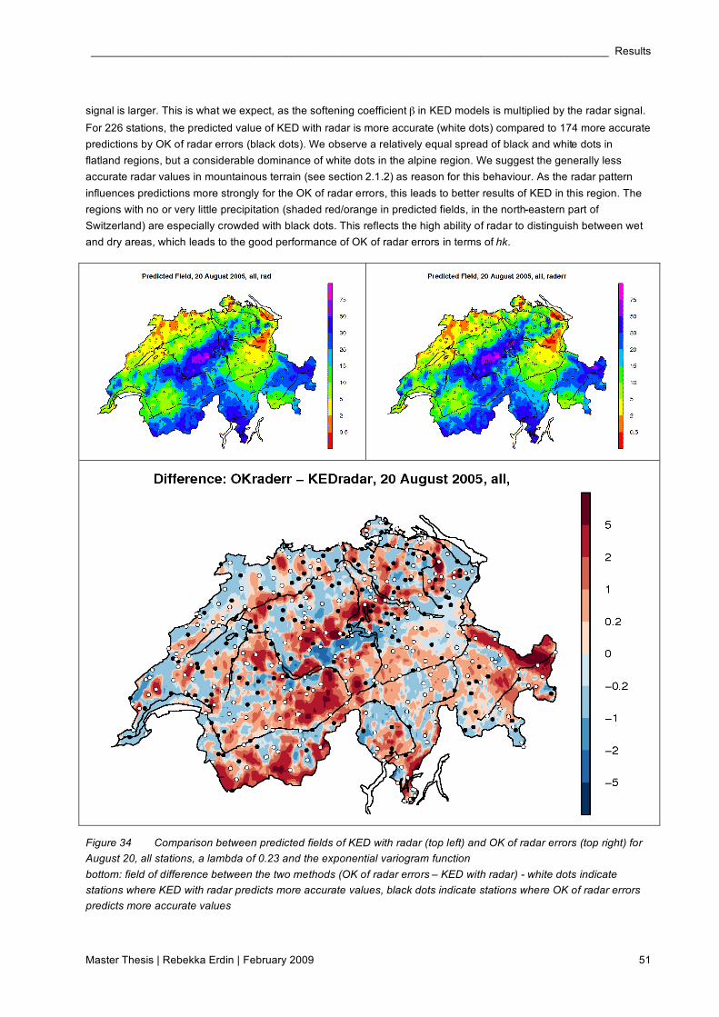
_____________________________________________________________________________________ Results
Master Thesis | Rebekka Erdin | February 2009 51
signal is larger. This is what we expect, as the softening coefficient ( in KED models is multiplied by the radar signal.
For 226 stations, the predicted value of KED with radar is more accurate (white dots) compared to 174 more accurate
predictions by OK of radar errors (black dots). We observe a relatively equal spread of black and white dots in
flatland regions, but a considerable dominance of white dots in the alpine region. We suggest the generally less
accurate radar values in mountainous terrain (see section 2.1.2) as reason for this behaviour. As the radar pattern
influences predictions more strongly for the OK of radar errors, this leads to better results of KED in this region. The
regions with no or very little precipitation (shaded red/orange in predicted fields, in the north-eastern part of
Switzerland) are especially crowded with black dots. This reflects the high ability of radar to distinguish between wet
and dry areas, which leads to the good performance of OK of radar errors in terms of hk.
Figure 34 Comparison between predicted fields of KED with radar (top left) and OK of radar errors (top right) for
August 20, all stations, a lambda of 0.23 and the exponential variogram function
bottom: field of difference between the two methods (OK of radar errors – KED with radar) - white dots indicate
stations where KED with radar predicts more accurate values, black dots indicate stations where OK of radar errors
predicts more accurate values
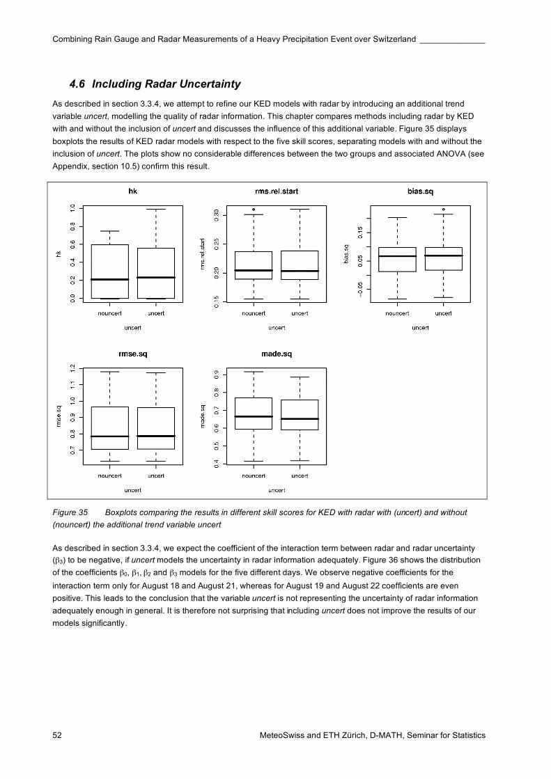
Combining Rain Gauge and Radar Measurements of a Heavy Precipitation Event over Switzerland ______________
52 MeteoSwiss and ETH Zürich, D-MATH, Seminar for Statistics
4.6 Including Radar Uncertainty
As described in section 3.3.4, we attempt to refine our KED models with radar by introducing an additional trend
variable uncert, modelling the quality of radar information. This chapter compares methods including radar by KED
with and without the inclusion of uncert and discusses the influence of this additional variable. Figure 35 displays
boxplots the results of KED radar models with respect to the five skill scores, separating models with and without the
inclusion of uncert. The plots show no considerable differences between the two groups and associated ANOVA (see
Appendix, section 10.5) confirm this result.
Figure 35 Boxplots comparing the results in different skill scores for KED with radar with (uncert) and without
(nouncert) the additional trend variable uncert
As described in section 3.3.4, we expect the coefficient of the interaction term between radar and radar uncertainty
((3) to be negative, if uncert models the uncertainty in radar information adequately. Figure 36 shows the distribution
of the coefficients (0, (1, (2 and (3 models for the five different days. We observe negative coefficients for the
interaction term only for August 18 and August 21, whereas for August 19 and August 22 coefficients are even
positive. This leads to the conclusion that the variable uncert is not representing the uncertainty of radar information
adequately enough in general. It is therefore not surprising that including uncert does not improve the results of our
models significantly.
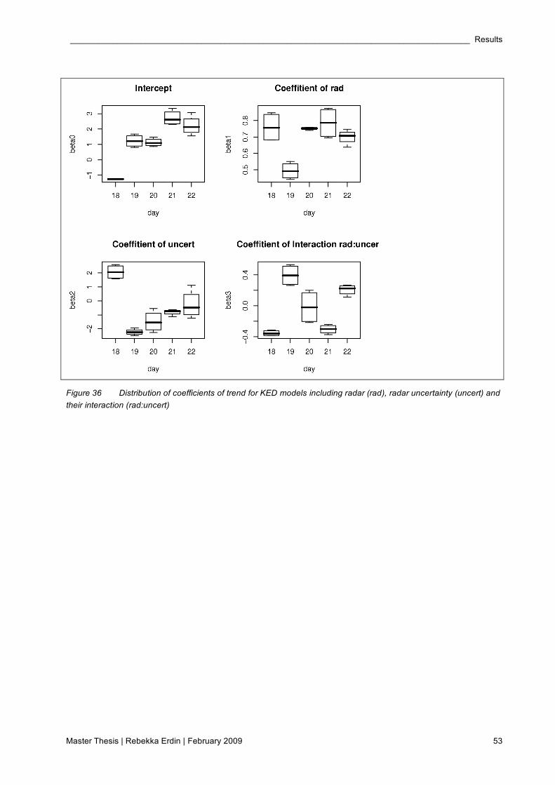
_____________________________________________________________________________________ Results
Master Thesis | Rebekka Erdin | February 2009 53
Figure 36 Distribution of coefficients of trend for KED models including radar (rad), radar uncertainty (uncert) and
their interaction (rad:uncert)

Combining Rain Gauge and Radar Measurements of a Heavy Precipitation Event over Switzerland ______________
54 MeteoSwiss and ETH Zürich, D-MATH, Seminar for Statistics

_____________________________________________________________________ Conclusions and Discussion
Master Thesis | Rebekka Erdin | February 2009 55
5 Conclusions and Discussion
This section summarizes and discusses the most important findings of the study. As we have seen in the preceding
section, examined combination methods are clearly capable to incorporate the accuracy of rain gauges and the high
spatial resolution of radar for our example case. The radar bias is eliminated in combined precipitation fields, i.e. their
biases are comparable to those of pure rain gauge fields. A particular strength of radar in distinguishing between wet
and dry areas has been discovered for the five analysed days. This ability of radar is well inherited by the combined
fields. We can therefore conclude that the examined methods combine the main strengths and mutually compensate
the main weaknesses of rain gauge and radar measurements in our case study.
Our combined fields exhibit better results in terms of all skill scores than pure rain gauge or pure radar fields. The
improvement compared to pure gauge fields is larger if we consider the less dense SMN gauge network only -
instead of the full station network - to build the models. This implies that including radar information can particularly
improve the resulting precipitation field if we work with a coarse gauge network. Combination methods show
therefore great promise for precipitation fields on shorter time scales, e.g. hourly precipitation, as only SMN stations
provide measurements on those time scales. However, shorter time scales might also pose additional challenges, as
will be discussed below (see section 6).
We evaluated our methods for five different days, including convective and stratiform precipitation situations. The
improvement of results by including radar information is larger for days with convective precipitation, i.e. for days with
more small-scale variation of precipitation. This is not very surprising, as the high spatial resolution of radar should
capture these small-scale variations, whereas they are often missed by the coarser resolution of the gauge network.
The precipitation situation has shown a large impact on all examined skill scores in our analyses of the systematic
evaluation of methods. It is therefore very important to consider its influence on the results, if we compare
precipitation fields of different days with each other. Otherwise effects of methodological factors could be masked by
differences between days.
The transformation of data prior to analyses seems to have an important impact on the resulting precipitation fields.
In our case study, this is particularly true for the ability of a model to distinguish between wet and dry areas. The
choice of transformation as well as transformation parameters is thus crucial to get satisfactory results. In addition,
different days have shown unequal behaviour of skill scores for the two examined transformation parameters. This
implies that distinct distributions of precipitation amounts might ask for customized transformation of data in order to
get optimal results.
The two examined parametric functions to model the variogram have no impact on the results in our case study. One
possible interpretation of this fact is that both functions represent the true covariance structure of a precipitation
pattern accurately enough – compared to other error sources – to include it for Kriging predictions in an appropriate
way. Regarding future applications of methods (e.g. applications on shorter time scales based on coarser gauge
networks), we expect to be faced with data sets of far less data pairs registering precipitation to model variograms
(see section 6). The observed robustness of results against different variogram models is therefore a convenient
finding with respect to those difficulties.
The two combination methods examined show relatively small but nevertheless clear differences in results. The more
flexible Kriging with external drift (KED) with radar as drift variable outperforms the Kriging (OK) of radar errors in
general. We therefore suggest this method as first choice to combine rain gauge and radar measurements for a
mountainous region such as Switzerland. The Kriging (OK) of radar errors, on the other hand, has shown a particular
strength in distinguishing between wet and dry areas, because of its broader inclusion of radar information. This me-
thod is therefore preferable if the ability to separate dry from wet areas is the main criterion in a specific application.
Combining Rain Gauge and Radar Measurements of a Heavy Precipitation Event over Switzerland ______________
56 MeteoSwiss and ETH Zürich, D-MATH, Seminar for Statistics
This study offered the possibility to compare the improvements of an additional inclusion of radar and 365 additional
rain gauge stations. Again the ability of radar to distinguish between dry and wet can be observed by the larger
added value by radar with respect to the corresponding skill score. In terms of skill scores measuring overall
performance, on the other hand, the added value of radar and additional rain gauges are of comparable size. This
comparison of added value by additional gauges or radar, however, depends on the precipitation situation. We
observe a particularly large relative added value by radar for the day with the most convective precipitation pattern.
We would like to point out that the comparison has to be handled with care, as the abundance of evaluation locations
over flatland in our study might favour methods including radar, because of the larger uncertainties of radar
measurements in mountainous areas.
The additional inclusion of radar uncertainty in models including radar by KED has not been successful in this study.
The coefficients of the interaction term in the trend are only partially of negative sign as expected. On top of that,
comparisons between models including radar uncertainty and the corresponding models including only radar show no
improvement of skill scores. We suggest that our approach to model radar uncertainty is not accurate enough to
improve combined precipitation fields. If this is the case, more sophisticated procedures to model radar uncertainty
could help to refine combination methods.
This is a case study and there are limitations to the generalisation of its results. First of all, the examined precipitation
situation is rather special. A heavy precipitation event of such degree occurs only rarely in Northern Switzerland. It
has to be pointed out that the large extent of precipitation during the examined days offers favourable conditions to
applied methods: There is no very pronounced peak at zero in the distributions of our untransformed data sets and
variogram modelling is facilitated by the abundance of data pairs registering positive precipitation. The results of our
study may therefore not be generalised one-to-one situations with pronounced small scale precipitation patterns.
Second, the time scale of daily precipitation sums of our study has to be taken into account. This time scale also
facilitates variogram estimation and therefore geostatistical methods, because dry stations are less abundant.
We compare our results to those of other authors performing similar combination methods in the following.
Haberlandt (2007), comparing geostatistical and other combination methods for hourly precipitation amounts, found
similar results for an extreme rainfall event over Germany as we did in our study. He concludes that precipitation
fields produced by KED including radar as drift variable clearly outperform univariate precipitation fields as well as
other combination methods. In addition he also finds that the impact of the modelled variogram on the results is not
very high. Velasco–Forero et al. (2004) combine gauges and radar by KED, but estimate the variogram by a non-
parametric method based on FFT. They find a good incorporation of the accuracy of gauges and the spatial
resolution of radar for their combined precipitation fields as well as an elimination of radar bias. Hence, our results
about KED with radar agree well with those mentioned above. Two studies performing combination of rain gauge and
radar by similar techniques as OK of radar errors (DeGaetano and Wilks, 2008; Jurczyk et al., 2007) find also
improvements of their combined fields compared to pure fields. However, none of the publications mentioned above
compares the OK of radar errors to KED with radar. We therefore agree about the general improvement of gauge
fields by the additional inclusion of radar, but cannot compare our results about the differences between the two
combination methods to those of other authors.
_____________________________________________________________________________________ Outlook
Master Thesis | Rebekka Erdin | February 2009 57
6 Outlook
This last section looks at open questions and recommended topics for future research concerning the combination of
rain gauge and radar measurements for the area of Switzerland.
Various hypotheses about strengths and weaknesses as well as influencing factors of the two presented combination
methods have been generated in this study. As a next step, the performance of these methods should be evaluated
systematically for a variety precipitation situations and over longer time periods in order to test these suggested
hypotheses. We expect that such an evaluation potentially poses a challenge to the geostatistical combination
methods of our study. The frequency of positive precipitation will be considerably lower than in our example case for
many days. Hence, less data pairs with valuable information about the autocorrelation are available to estimate
variogram parameters. In addition, this pronounced peak at zero in precipitation distribution could lead to problems in
finding an appropriate transformation of data in order to fulfil model assumptions for MLE of model parameters.
All analyses in this study were conducted on daily time scale. Yet, precipitation fields on shorter time scales, e.g.
hourly precipitation, are of interest for many applications. It would therefore be interesting to apply the geostatistical
combination methods presented in this study to precipitation data on hourly or even shorter time scale. However, the
challenges mentioned in the subsection above are expected to be even larger in this situation. First, because the
available gauge network is less dense, because only the automatic stations are measuring precipitation on shorter
than daily time scales. Second, the relative abundance of dry stations is expected to increase with shorter time
scales, because there is less aggregation of dry and wet time intervals for each location. We therefore anticipate a
potential need for other estimation procedures or even new combination techniques for applications on shorter time
scales.
Our first approach to model radar uncertainty in this study has not been successful. Nevertheless, the idea to include
information about the local quality of radar information would be interesting to pursue in further research, as
differences in radar accuracy between mountains and flatlands are widely observed. More sophisticated modelling
techniques might generate fields of radar uncertainty with the resolution needed. The inclusion of this information
could improve the resulting combined precipitation fields. On top of that, such appropriate uncertainty fields could
enable different combination approaches such as Bayesian techniques mentioned below in this section.
The comparison between the two examined methods in this study has lead to the hypothesis that the advantage of
the more flexible KED with radar over OK of radar errors is particularly pronounced in mountainous regions. We
suggested its attenuation of the radar signal by a coefficient ( smaller than 1 as the reason for this observation,
because the bias of radar measurements is known to be particularly severe in mountainous terrain. Further
investigations in this area would be of interest in order to develop and analyse methods to divide Switzerland into
different regions and allow various coefficients ( to model precipitation. This approach would point in the same
direction as the inclusion of information about radar uncertainty, but by a different technique.
Another idea is to model distances between gauge stations not in terms of Euclidean distances as given by
geographical coordinates, but in a more sophisticated way. A similarity measure accounting for climatologically
observed or physically plausible similarities and dissimilarities of precipitation amounts could be constructed to model
the distance between locations. This measure could for instance incorporate information about topography or the
classification into different climatological regions beside the geographical distance.
We postulate the hypothesis of a particular strength of radar to distinguish between dry and wet in this study. The
further exploration of this strength would be an important next step. If the hypothesis can be approved, this could
offer the possibility of new combination techniques, benefiting from this particular ability of radar measurements. A
first approach could be the simple correction of modelled precipitation fields by the wet-dry-pattern of radar fields.

Combining Rain Gauge and Radar Measurements of a Heavy Precipitation Event over Switzerland ______________
58 MeteoSwiss and ETH Zürich, D-MATH, Seminar for Statistics
The idea of Double Optimal Estimation (DOE) as described in section 3.3.3 has not been implemented finally in this
study because of theoretical obstacles. Yet we consider the general concept to model the probability of precipitation
independently from the expected precipitation amount conditional to positive precipitation as potentially promising. It
would therefore be interesting to further pursue this idea. We suggest that if DOE will be implemented in the future,
this method could be promising to profit in a more elaborate manner from the good ability of radar to distinguish
between wet and dry areas. This could be achieved by including radar especially for the modelling of the probability
of precipitation, where a sharp distinction between wet and dry is of great value. An idea for the technical
implementation of the first step of DOE is to use the logistic function to model the probability of precipitation.
Beside further evaluations and refinements of methods presented or mentioned in this study, it would be interesting
to analyse alternative methodological approaches to combine rain gauge and radar measurements. There are, for
instance, promising combination techniques based on Bayesian frameworks found in literature. Todini (2001) et al.
combine Block Kriging and Kalman filtering in a Bayesian way in order to introduce gauge and radar data according
to their relative uncertainties. Fuentes et al. (2008) combine rain gauge and radar measurements in a Bayesian way
by introducing them in terms of an underlying latent process of true precipitation values. They use spatial logistic
regression to model the probability of precipitation for the two data sources.
For many applications, precipitation fields should be available in real-time. The feasibility of real-time applications
should therefore be considered in future development of combination methods, as this offers particular challenges to
applied methods. If Kriging appears to be the preferable combination method, it might be interesting to assess the
possibility of non-parametric variogram modelling technique based on Fast Fourier Transform (FFT) as suggested by
Velasco-Forero et al. (2004).
Overall, we see a strong potential in the combination of rain gauge and radar measurements with regard to several
applications. First of all, combination methods show great promise for the generation of real-time precipitation fields
that satisfy the growing needs of many users in terms of accuracy and resolution. Second, they might be useful to
refine procedures checking data quality, as implausible measurements could be identified by combined precipitation
fields (see example in section 4.4.3). In addition, combined precipitation fields could be employed to examine the
representativity of current measurement networks and define effective measures for their improvement in the future.
MeteoSwiss is currently planning two projects related to the research topic: Rad4Alps and CombiPrecip. Rad4Alps
aims at the renewal and possible expansion of the radar network. The quality of radar data at MeteoSwiss might thus
even improve in the future. This is a promising development as we expect combined precipitation fields to benefit
from such an improvement. In addition, more accurate radar fields might even offer the possibility for new
combination approaches. The subproject CombiPrecip of MeteoSwiss is embedded in the project NCCR Climate III, a
Swiss Research Network of various institutions. The aim of CombiPrecip is to develop appropriate methods to
combine rain gauge and radar measurements in real-time for different time scales. This includes further
developments based on this study such as a broader evaluation of presented methods and the assessment of
methods for shorter time scales as well as the analysis of additional combination methods. CombiPrecip is thus going
to pursue many of the open questions and ideas presented in this section.

___________________________________________________________________________ Acknowledgements
Master Thesis | Rebekka Erdin | February 2009 59
7 Acknowledgements
I would like to particularly thank my supervisor Christoph Frei from MeteoSwiss and my supervising Professor Werner
Stahel from ETH Zurich for their advice and support during my master thesis. I could benefit a lot from their
experience and ideas and I especially enjoyed the numerous inspiring discussions about the subject of my thesis that
we shared.
Thanks are also given to all the other persons who supported and helped me with my study along the way –
especially Andreas Papritz and Prof H.R. Künsch from ETH Zurich as well as Urs Germann, Reinhard Schiemann
and Sophie Fukutome from MeteoSwiss.
In addition, I want to generally thank MeteoSwiss for providing the data as well as competent advisors and a pleasant
and motivating working environment.
Last but not least I would like to thank my parents, my parents-in-law and especially my husband for sharing the care
of our daughter and supporting me in every way – it is them who enabled me to finish my studies and write this
thesis.

Combining Rain Gauge and Radar Measurements of a Heavy Precipitation Event over Switzerland ______________
60 MeteoSwiss and ETH Zürich, D-MATH, Seminar for Statistics
___________________________________________________________________________________ Literature
Master Thesis | Rebekka Erdin | February 2009 61
8 Literature
Barancourt, C. & Creutin, J. D. (1992), 'A Method for Delineating and Estimating Rainfall Fields’, Water Resources
Research 28(4), 1133-1144.
Bezzola, G. R. & Hegg, C. (2008), 'Ereignisanalyse Hochwasser 2005, Teil 2 - Analyse von Prozessen, Massnahmen
und Gefahrengrundlagen', Umwelt-Wissen (BAFU) 0825, 429.
Bezzola, G. R. & Hegg, C. (2007), 'Ereignisanalyse Hochwasser 2005, Teil 1 - Prozesse, Schäden und erste
Einordnung', Umwelt-Wissen (BAFU) 0707, 215.
Box, G. E. P. & Cox, D. R. (1964), 'An Analysis of Transformations', Journal of the Royal Statistical Society 26, 211-
252.
Cressie, N. A. C. (1993), Statistics for Spatial Data, Wiley, New York.
DeGaetano, A. T. & Wilks, D. S. (2008), 'Radar-guided interpolation of climatological precipitation data', International
Journal of Climatology DOI: 101002/joc.1714.
Diggle, P. J. & Ribeiro Jr., P. J. (2007), Model-based Geostatistics, Springer Science + Business Media, New York.
Frei, C.; Germann, U.; Fukutome, S. & Liniger, M. (2008), 'Möglichkeiten und Grenzen der Niederschlagsanalysen
zum Hochwasser 2005', Arbeitsberichte der MeteoSchweiz 221, 19.
Frei, C. & Schär, C. (1998), 'A Precipitation Climatology of the Alps from High-resolution Rain-gauge Observations',
International Journal of Climatology 18, 873-900.
Fuentes, M.; Reich, B. & Lee, G. (2008), 'Spatial-temporal mesoscale modeling of rainfall intensity using gage and
radar data', Annals of Applied Statistics 2, Number 4, 1148-1169.
Germann, U.; Galli, G.; Boscacci, M. & Bolliger, M. (2006), 'Radar precipitation measurement in a mountainous
region', Q. J. R. Meteorol. Soc. 132, 1669-1692.
Germann, U. & Joss, J. (2002), 'Mesobeta profiles to extrapolate radar precipitation measurements above the Alps to
the ground level', Journal of Applied Meteorology 41, 542-557.
Gjertsen, U.; Salek, M. & Michelson, D. B. (2004), 'Gauge adjustment of radar-based precipitation estimates in
Europe''3rd European Conference on Radar Meteorology and Hydrology (ERAD)'.
Haberlandt, U. (2007), 'Geostatistical interpolation of hourly precipitation from rain gauges and radar for a large-scale
extreme rainfall event', Journal of Hydrology 332, 144-157.
Joss, J. & Lee, R. (1995), 'The Application of Radar-Gauge Comparisons to Operational Precipitation Profile
Corrections', Journal of Applied Meteorology 34, 2612-2630.
Jurczyk, A.; Osrodka, K. & Szturc, J. (2007), 'Research studies on improvement in real-time estimation of radar-
based precipitation in Poland', Meteorology and Atmospheric Physics DOI 10.1007/s00703-007-0266-3.
Marshall, J.; Langille, R. & W.McK., P. (1947), 'Measurement of Rainfall by Radar', Journal of Meteorology 4, 186-
192.
MeteoSchweiz (2006), 'Starkniederschlagsereignis August 2005', Arbeitsbericht MeteoSchweiz 211.
Papritz, A. (2008), 'Einführung in die lineare Geostatistik', lecture notes.
Papritz, A. (2008), personal communication (meeting) on December 17., 2008.
Combining Rain Gauge and Radar Measurements of a Heavy Precipitation Event over Switzerland ______________
62 MeteoSwiss and ETH Zürich, D-MATH, Seminar for Statistics
Papritz, A.; Herzig, C.; Borer, F. & Bono, R. (2005), Geostatistics for Environmental Applications, Springer Verlag,
chapter Modelling the spatial distribution of copper in the soils around a metal smelter in northwestern
Switzerland, pp. 343-354.
Paulat, M.; Frei, C.; Hagen, M. & Wernli, H. (2009), in press, 'A gridded dataset of hourly precipitation in Germany its
construction, climatology and applications'.
R Development Core Team (2008), 'R: A language and environment for statistical computing’, R Foundation for
Statistical Computing, Vienna, Austria, ISBN 3-900051-07-0, URL http://www.R-project.org.
Ribeiro Jr., P.J. & Diggle, P.J. (2001), 'geoR: A package for geostatistical analysis', R-NEWS 1(2), 15-18. ISSN 1609-
3631.
Schmutz, C.; Arpagaus, M.; Clementi, L.; Frei, C.; Fukutome, S.; Germann, U.; Liniger, M. & Schacher, F. (2008),
'Meteorologische Ereignisanalyse des Hochwassers 8. bis 9. August 2007', Arbeitsbericht MeteoSchweiz 222,
30 pp..
Seo, D. (1998), 'Real-time estimation of rainfall fields using radar rainfall and rain gage data', Journal of Hydrology
208, 37-52.
Seo, D. (1998), 'Real-time estimation of rainfall fields using rain gage data under fractional coverage conditions',
Journal of Hydrology 208, 25-36.
Sevruk, B. (1985), 'Systematischer Niederschlagsmessfehler in der Schweiz', Beitr. Geol. Schweiz - Hydrol. 31.
Stahel, W., ed. (2008), Statistische Datenanalyse, Vieweg + Teubner.
Stahel, W. (2008), personal communication (e-mail) on December 5., 2008.
Stahel, W. (2006), 'Lineare Regression', Lecture Notes.
Todini, E. (2001), 'A Bayesian technique for conditioning radar precipitation estimates to rain-gauge measurements',
Hydrology and Earth System Sciences 5(2), 187-199.
Velasco-Forero, C.; Cassiraga, E. F.; Sempere-Torres, D.; Sanchez-Diezma, R. & Gomez-Hernandez, J. J. (2004), 'A
non-parametric methodology to merge raingauges and radar by kriging: sensitivity to errors in radar
measurements''3rd European Conference on Radar in Meteorology and Hydrology (ERAD)'.
Webster, R. & Oliver, M. S. (2007), Geostatistics for Environmental Scientists, Wiley, New York.
Wüest, M.; Frei, C.; Altenhoff, A.; Hagen, M.; Litschi, M. & Schär, C. (2009), submitted, 'A gridded hourly precipitation
dataset for Switzerland using rain-gauge analysis and radar-based disaggregation'.
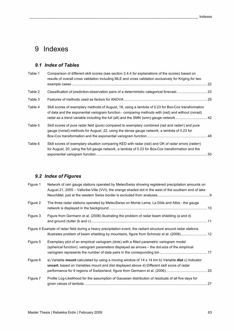
_____________________________________________________________________________________ Indexes
Master Thesis | Rebekka Erdin | February 2009 63
9 Indexes
9.1 Index of Tables
Table 1 Comparison of different skill scores (see section 3.4.4 for explanations of the scores) based on
results of overall cross validation including MLE and cross validation exclusively for Kriging for two
example cases ............................................................................................................................................... 22
Table 2 Classification of prediction-observation pairs of a deterministic categorical forecast................................ 23
Table 3 Features of methods used as factors for ANOVA........................................................................................ 25
Table 4 Skill scores of exemplary methods of August, 18, using a lambda of 0.23 for Box-Cox transformation
of data and the exponential variogram function - comparing methods with (rad) and without (norad)
radar as a trend variable including the full (all) and the SMN (smn) gauge network ................................. 42
Table 5 Skill scores of pure radar field (pure) compared to exemplary combined (rad and raderr) and pure
gauge (norad) methods for August, 22, using the dense gauge network, a lambda of 0.23 for
Box-Cox transformation and the exponential variogram function ............................................................... 48
Table 6 Skill scores of exemplary situation comparing KED with radar (rad) and OK of radar errors (raderr)
for August, 20, using the full gauge network, a lambda of 0.23 for Box-Cox transformation and the
exponential variogram function ..................................................................................................................... 50
9.2 Index of Figures
Figure 1 Network of rain gauge stations operated by MeteoSwiss showing registered precipitation amounts on
August 21, 2005 – Vallorbe-Ville (VVI), the orange shaded dot in the west of the southern end of lake
Neuchâtel, just at the western Swiss border is excluded from analyses.......................................................9
Figure 2 The three radar stations operated by MeteoSwiss on Monte Lema, La Dôle and Albis - the gauge
network is displayed in the background........................................................................................................ 10
Figure 3 Figure from Germann et al. (2006) illustrating the problem of radar beam shielding (a and d)
and ground clutter (b and c) .......................................................................................................................... 11
Figure 4 Example of radar field during a heavy precipitation event, the radiant structure around radar stations
illustrates problem of beam shielding by mountains, figure from Schmutz et al. (2008) ........................... 12
Figure 5 Exemplary plot of an empirical variogram (dots) with a fitted parametric variogram model
(spherical function), variogram parameters displayed as arrows – the dot-size of the empirical
variogram represents the number of data pairs in the corresponding bin .................................................. 17
Figure 6 a) Variable mount calculated by using a moving window of 14 x 14 km b) Variable dist c) Indicator
uncert, based on Variables mount and dist displayed above d) Different skill score of radar
performance for 9 regions of Switzerland, figure from Germann et al. (2006) ........................................... 20
Figure 7 Profile Log-Likelihood for the assumption of Gaussian distribution of residuals of all five days for
given values of lambda .................................................................................................................................. 27
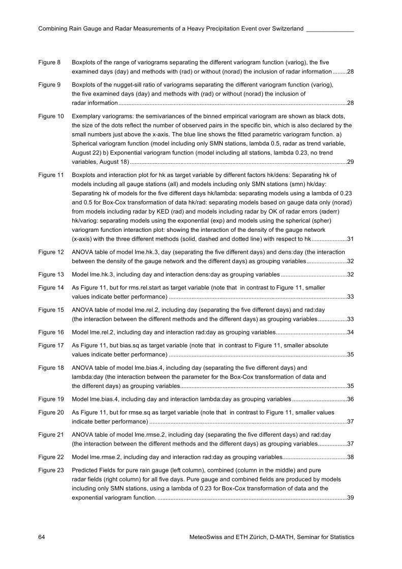
Combining Rain Gauge and Radar Measurements of a Heavy Precipitation Event over Switzerland ______________
64 MeteoSwiss and ETH Zürich, D-MATH, Seminar for Statistics
Figure 8 Boxplots of the range of variograms separating the different variogram function (variog), the five
examined days (day) and methods with (rad) or without (norad) the inclusion of radar information .........28
Figure 9 Boxplots of the nugget-sill ratio of variograms separating the different variogram function (variog),
the five examined days (day) and methods with (rad) or without (norad) the inclusion of
radar information.............................................................................................................................................28
Figure 10 Exemplary variograms: the semivariances of the binned empirical variogram are shown as black dots,
the size of the dots reflect the number of observed pairs in the specific bin, which is also declared by the
small numbers just above the x-axis. The blue line shows the fitted parametric variogram function. a)
Spherical variogram function (model including only SMN stations, lambda 0.5, radar as trend variable,
August 22) b) Exponential variogram function (model including all stations, lambda 0.23, no trend
variables, August 18) ......................................................................................................................................29
Figure 11 Boxplots and interaction plot for hk as target variable by different factors hk/dens: Separating hk of
models including all gauge stations (all) and models including only SMN stations (smn) hk/day:
Separating hk of models for the five different days hk/lambda: separating models using a lambda of 0.23
and 0.5 for Box-Cox transformation of data hk/rad: separating models based on gauge data only (norad)
from models including radar by KED (rad) and models including radar by OK of radar errors (raderr)
hk/variog: separating models using the exponential (exp) and models using the spherical (spher)
variogram function interaction plot: showing the interaction of the density of the gauge network
(x-axis) with the three different methods (solid, dashed and dotted line) with respect to hk......................31
Figure 12 ANOVA table of model lme.hk.3, day (separating the five different days) and dens:day (the interaction
between the density of the gauge network and the different days) as grouping variables.........................32
Figure 13 Model lme.hk.3, including day and interaction dens:day as grouping variables .........................................32
Figure 14 As Figure 11, but for rms.rel.start as target variable (note that in contrast to Figure 11, smaller
values indicate better performance) ..............................................................................................................33
Figure 15 ANOVA table of model lme.rel.2, including day (separating the five different days) and rad:day
(the interaction between the different methods and the different days) as grouping variables..................33
Figure 16 Model lme.rel.2, including day and interaction rad:day as grouping variables............................................34
Figure 17 As Figure 11, but bias.sq as target variable (note that in contrast to Figure 11, smaller absolute
values indicate better performance) ..............................................................................................................35
Figure 18 ANOVA table of model lme.bias.4, including day (separating the five different days) and
lambda:day (the interaction between the parameter for the Box-Cox transformation of data and
the different days) as grouping variables.......................................................................................................35
Figure 19 Model lme.bias.4, including day and interaction lambda:day as grouping variables ..................................36
Figure 20 As Figure 11, but for rmse.sq as target variable (note that in contrast to Figure 11, smaller values
indicate better performance) ..........................................................................................................................37
Figure 21 ANOVA table of model lme.rmse.2, including day (separating the five different days) and rad:day
(the interaction between the different methods and the different days) as grouping variables..................37
Figure 22 Model lme.rmse.2, including day and interaction rad:day as grouping variables........................................38
Figure 23 Predicted Fields for pure rain gauge (left column), combined (column in the middle) and pure
radar fields (right column) for all five days. Pure gauge and combined fields are produced by models
including only SMN stations, using a lambda of 0.23 for Box-Cox transformation of data and the
exponential variogram function. .....................................................................................................................39
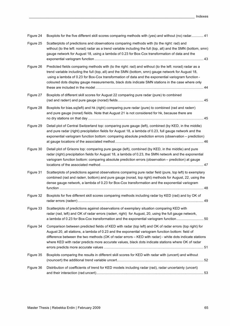
_____________________________________________________________________________________ Indexes
Master Thesis | Rebekka Erdin | February 2009 65
Figure 24 Boxplots for the five different skill scores comparing methods with (yes) and without (no) radar............. 41
Figure 25 Scatterplots of predictions and observations comparing methods with (to the right: rad) and
without (to the left: norad) radar as a trend variable including the full (top, all) and the SMN (bottom, smn)
gauge network for August 18, using a lambda of 0.23 for Box-Cox transformation of data and the
exponential variogram function ..................................................................................................................... 43
Figure 26 Predicted fields comparing methods with (to the right: rad) and without (to the left: norad) radar as a
trend variable including the full (top, all) and the SMN (bottom, smn) gauge network for August 18,
using a lambda of 0.23 for Box-Cox transformation of data and the exponential variogram function -
coloured dots display gauge measurements, black dots indicate SMN stations in the case where only
these are included in the model .................................................................................................................... 44
Figure 27 Boxplots of different skill scores for August 22 comparing pure radar (pure) to combined
(rad and raderr) and pure gauge (norad) fields............................................................................................ 45
Figure 28 Boxplots for bias.sq(left) and hk (right) comparing pure radar (pure) to combined (rad and raderr)
and pure gauge (norad) fields. Note that August 21 is not considered for hk, because there are
no dry stations on that day ............................................................................................................................ 45
Figure 29 Detail plot of Central Switzerland top: comparing pure gauge (left), combined (by KED, in the middle)
and pure radar (right) precipitation fields for August 18, a lambda of 0.23, full gauge network and the
exponential variogram function bottom: comparing absolute prediction errors (observation – prediction)
at gauge locations of the associated method............................................................................................... 46
Figure 30 Detail plot of Grisons top: comparing pure gauge (left), combined (by KED, in the middle) and pure
radar (right) precipitation fields for August 18, a lambda of 0.23, the SMN network and the exponential
variogram function bottom: comparing absolute prediction errors (observation – prediction) at gauge
locations of the associated method............................................................................................................... 47
Figure 31 Scatterplots of predictions against observations comparing pure radar field (pure, top left) to exemplary
combined (rad and raderr, bottom) and pure gauge (norad, top right) methods for August, 22, using the
dense gauge network, a lambda of 0.23 for Box-Cox transformation and the exponential variogram
function ........................................................................................................................................................... 48
Figure 32 Boxplots for five different skill scores comparing methods including radar by KED (rad) and by OK of
radar errors (raderr) ....................................................................................................................................... 49
Figure 33 Scatterplots of predictions against observations of exemplary situation comparing KED with
radar (rad, left) and OK of radar errors (raderr, right) for August, 20, using the full gauge network,
a lambda of 0.23 for Box-Cox transformation and the exponential variogram function............................. 50
Figure 34 Comparison between predicted fields of KED with radar (top left) and OK of radar errors (top right) for
August 20, all stations, a lambda of 0.23 and the exponential variogram function bottom: field of
difference between the two methods (OK of radar errors – KED with radar) - white dots indicate stations
where KED with radar predicts more accurate values, black dots indicate stations where OK of radar
errors predicts more accurate values ........................................................................................................... 51
Figure 35 Boxplots comparing the results in different skill scores for KED with radar with (uncert) and without
(nouncert) the additional trend variable uncert............................................................................................. 52
Figure 36 Distribution of coefficients of trend for KED models including radar (rad), radar uncertainty (uncert)
and their interaction (rad:uncert) ................................................................................................................... 53
Combining Rain Gauge and Radar Measurements of a Heavy Precipitation Event over Switzerland ______________
66 MeteoSwiss and ETH Zürich, D-MATH, Seminar for Statistics
9.3 Index of Abbreviations and Variable Names
a coefficient for the transformation of radar reflectivity Z into a rain rate R
ACC accuracy
ANOVA Analysis of Variance
b coefficient for the transformation of radar reflectivity Z into a rain rate R
bias.sq systematic error based on square root transformed values, skill score
BLUP best linear unbiased predictor
C() autocovariance
cov{} covariance
day variable indicating the examined day in August 2005, categories: 18, 19, 20, 21, 22
dens variable indicating the density of the involved rain gauge network, categories: all (full station network of 440 gauges), smn (75 SMN stations only)
dist variable based on the Euclidean distance from the closest radar station
DOE double optimal estimation
E{} expected value
ETH Swiss Federal Institute of Technology
FFT Fast Fourier Transform
h lag, distance between two points
hk hanssen kuipers discriminant, skill score
i index for spatial reference
IDW inverse distance weighting
IK Indicator Kriging
j index for one of n gauge stations
KED Kriging with external drift
lambda variable indicating parameter chosen for Box-Cox transformation, categories: 0.23, 0.5
log logarithm
MAD mean absolute deviation
made.sq 1.4826 times the mean absolute deviation based on square root transformed values, skill score
MLE maximum likelihood estimation
mount variable based on the roughness of topography
Obs Observation
OK Ordinary Kriging
Pred Prediction
QQ Quantile-Quantile
R radar errors or rain rate, depending on the context
r() autocorrelation
rad variable indicating the geostatistical method applied, categories: norad (OK of rain gauges), rad (KED with radar as trend variable), raderr(OK of radar errors), pure (pure radar field, no Kriging)
REML restricted maximum likelihood estimation
RMS root mean square
RMSE root mean squared error

_____________________________________________________________________________________ Indexes
Master Thesis | Rebekka Erdin | February 2009 67
rmse.sq root mean squared error based on square root transformed values, skill score
rms.rel.start root mean square of relative error based on started logs, skill score
s vector of coordinates, spatial reference
SK Simple Kriging
SMN SwissMetNet, network of automatic meteorological measurement stations
SS skill score
U radar uncertainty
UK Universal Kriging
uncert variable modelling the uncertainty of radar measurements, based on mount and dist
UTC Coordinated Universal Time
var{} variance
variog variable indicating the parametric function chosen to model the variogram, categories: exp (exponential), spher (spherical)
VVI manually operated rain gauge at Vallorbe-Ville
X radar measurements
Y rain gauge measurements
Z modelled precipitation amount or radar reflectivity, depending on the context
' coefficient of intercept in linear trend models
( coefficient of trend variables in linear trend models
) term in Kriging prediction, weighted sum of deviations of observations from trend
$ semivariance
" parameter of Box-Cox transformation family
µ mean

Combining Rain Gauge and Radar Measurements of a Heavy Precipitation Event over Switzerland ______________
68 MeteoSwiss and ETH Zürich, D-MATH, Seminar for Statistics

____________________________________________________________________________________ Appendix
Master Thesis | Rebekka Erdin | February 2009 69 69
10 Appendix
10.1 Box-Cox Transformation..............................................70
10.2 Analyses of Variance....................................................72
10.2.1 HK........................................................................ 72
10.2.2 Rms.rel.start........................................................ 75
10.2.3 Bias.sq................................................................. 77
10.2.4 RMSE.SQ............................................................ 78
10.2.5 MADE.SQ............................................................ 82
10.3 Comparison between Combined and Pure Fields ...85
10.3.1 Combined versus Pure Gauge Fields ............... 85
10.3.2 Combined versus Pure Radar Fields ................ 87
10.3.3 Example August 18 ............................................ 90
10.3.4 Example August 22 ............................................ 96
10.4 Comparison between Combination Methods .........104
10.5 Including Radar Uncertainty......................................108
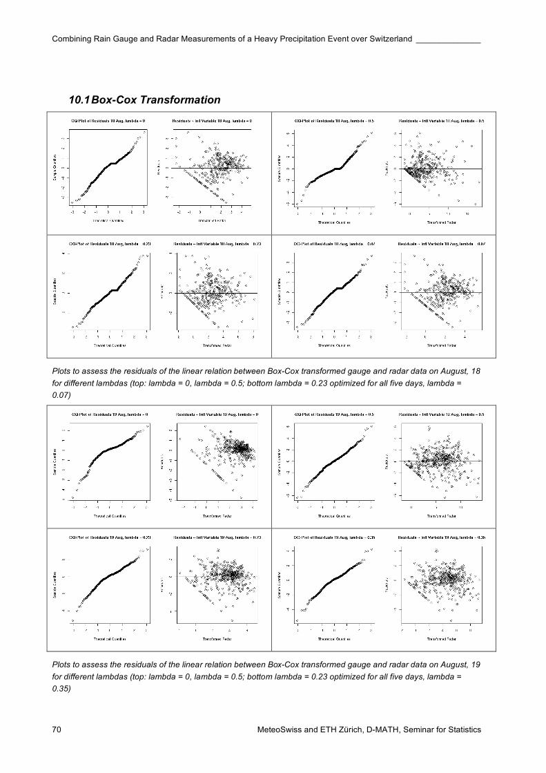
Combining Rain Gauge and Radar Measurements of a Heavy Precipitation Event over Switzerland ______________
MeteoSwiss and ETH Zürich, D-MATH, Seminar for Statistics 70
10.1 Box-Cox Transformation
Plots to assess the residuals of the linear relation between Box-Cox transformed gauge and radar data on August, 18
for different lambdas (top: lambda = 0, lambda = 0.5; bottom lambda = 0.23 optimized for all five days, lambda =
0.07)
Plots to assess the residuals of the linear relation between Box-Cox transformed gauge and radar data on August, 19
for different lambdas (top: lambda = 0, lambda = 0.5; bottom lambda = 0.23 optimized for all five days, lambda =
0.35)
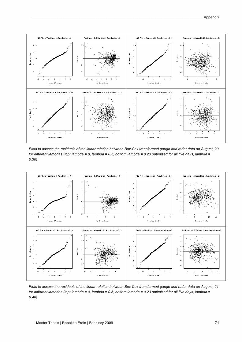
____________________________________________________________________________________ Appendix
Master Thesis | Rebekka Erdin | February 2009 71 71
Plots to assess the residuals of the linear relation between Box-Cox transformed gauge and radar data on August, 20
for different lambdas (top: lambda = 0, lambda = 0.5; bottom lambda = 0.23 optimized for all five days, lambda =
0.30)
Plots to assess the residuals of the linear relation between Box-Cox transformed gauge and radar data on August, 21
for different lambdas (top: lambda = 0, lambda = 0.5; bottom lambda = 0.23 optimized for all five days, lambda =
0.48)

Combining Rain Gauge and Radar Measurements of a Heavy Precipitation Event over Switzerland ______________
MeteoSwiss and ETH Zürich, D-MATH, Seminar for Statistics 72
Plots to assess the residuals of the linear relation between Box-Cox transformed gauge and radar data on August, 22
for different lambdas (top: lambda = 0, lambda = 0.5; bottom lambda = 0.23 optimized for all five days, lambda =
0.27)
10.2 Analyses of Variance
10.2.1 HK
Likelihood Ratio Test comparing models for skill score hk: lm.hk without the inclusion of grouping variables and
model lme.hk.1 including day as grouping variable
Likelihood Ratio Test comparing models for skill score hk: lme.hk.1 including day as grouping variable and model
lme.hk.3 including additionally dens:day as second grouping variable
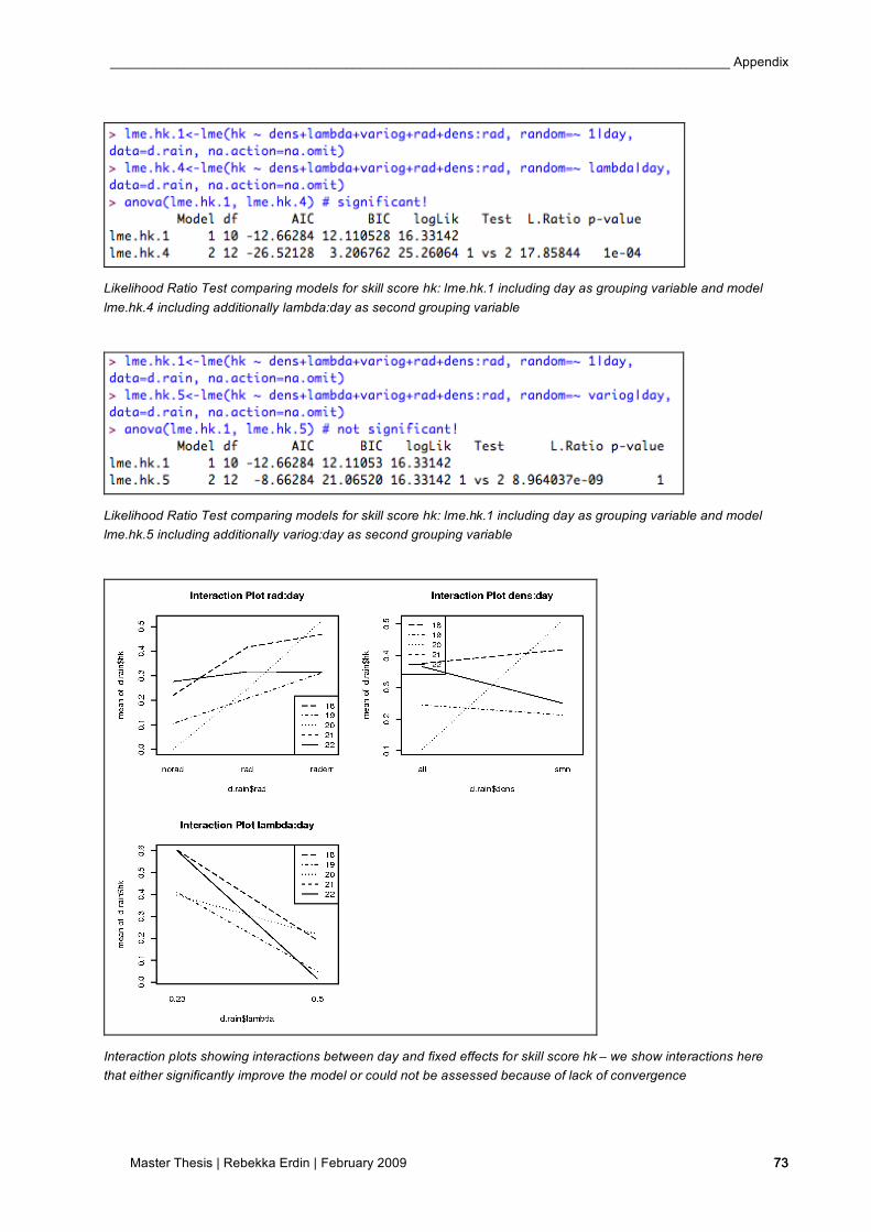
____________________________________________________________________________________ Appendix
Master Thesis | Rebekka Erdin | February 2009 73 73
Likelihood Ratio Test comparing models for skill score hk: lme.hk.1 including day as grouping variable and model
lme.hk.4 including additionally lambda:day as second grouping variable
Likelihood Ratio Test comparing models for skill score hk: lme.hk.1 including day as grouping variable and model
lme.hk.5 including additionally variog:day as second grouping variable
Interaction plots showing interactions between day and fixed effects for skill score hk – we show interactions here
that either significantly improve the model or could not be assessed because of lack of convergence
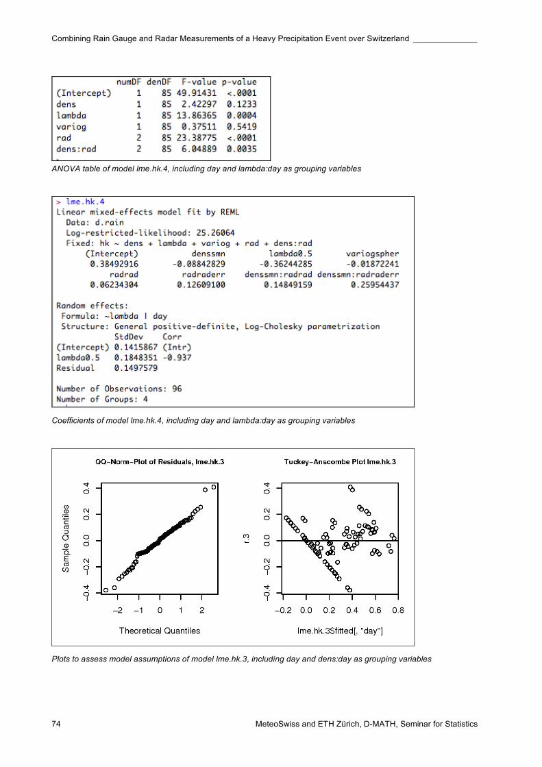
Combining Rain Gauge and Radar Measurements of a Heavy Precipitation Event over Switzerland ______________
MeteoSwiss and ETH Zürich, D-MATH, Seminar for Statistics 74
ANOVA table of model lme.hk.4, including day and lambda:day as grouping variables
Coefficients of model lme.hk.4, including day and lambda:day as grouping variables
Plots to assess model assumptions of model lme.hk.3, including day and dens:day as grouping variables
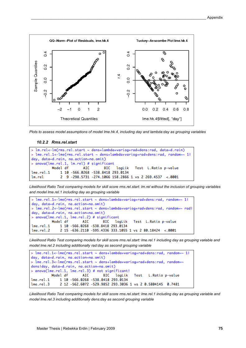
____________________________________________________________________________________ Appendix
Master Thesis | Rebekka Erdin | February 2009 75 75
Plots to assess model assumptions of model lme.hk.4, including day and lambda:day as grouping variables
10.2.2 Rms.rel.start
Likelihood Ratio Test comparing models for skill score rms.rel.start: lm.rel without the inclusion of grouping variables
and model lme.rel.1 including day as grouping variable
Likelihood Ratio Test comparing models for skill score rms.rel.start: lme.rel.1 including day as grouping variable and
model lme.rel.2 including additionally rad:day as second grouping variable
Likelihood Ratio Test comparing models for skill score rms.rel.start: lme.rel.1 including day as grouping variable and
model lme.rel.3 including additionally dens:day as second grouping variable
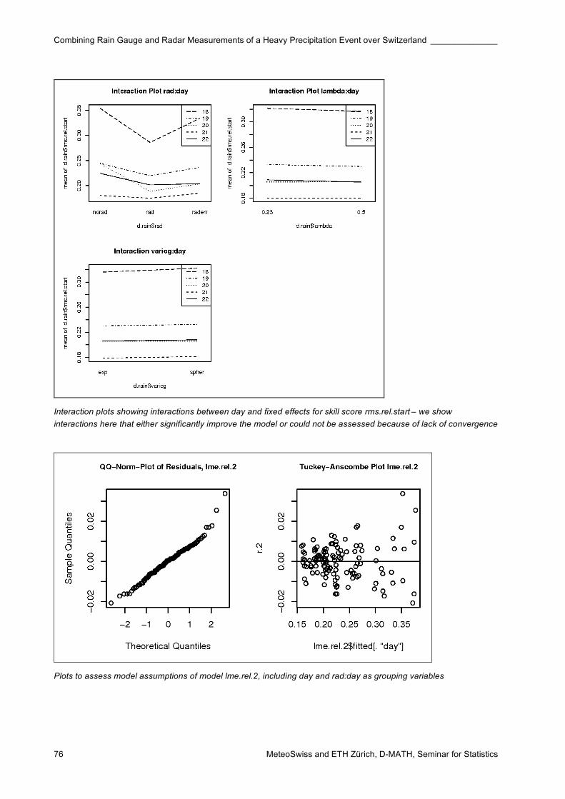
Combining Rain Gauge and Radar Measurements of a Heavy Precipitation Event over Switzerland ______________
MeteoSwiss and ETH Zürich, D-MATH, Seminar for Statistics 76
Interaction plots showing interactions between day and fixed effects for skill score rms.rel.start – we show
interactions here that either significantly improve the model or could not be assessed because of lack of convergence
Plots to assess model assumptions of model lme.rel.2, including day and rad:day as grouping variables

____________________________________________________________________________________ Appendix
Master Thesis | Rebekka Erdin | February 2009 77 77
10.2.3 Bias.sq
Likelihood Ratio Test comparing models for skill score bias.sq: lm.bias without the inclusion of grouping variables and
model lme.bias.1 including day as grouping variable
Likelihood Ratio Test comparing models for skill score bias.sq: lme.bias.1 including day as grouping variable and
model lme.bias.3 including additionally dens:day as second grouping variable
Likelihood Ratio Test comparing models for skill score bias.sq: lme.bias.1 including day as grouping variable and
model lme.bias.4 including additionally lambda:day as second grouping variable
Likelihood Ratio Test comparing models for skill score bias.sq: lme.bias.1 including day as grouping variable and
model lme.bias.5 including additionally variog:day as second grouping variable
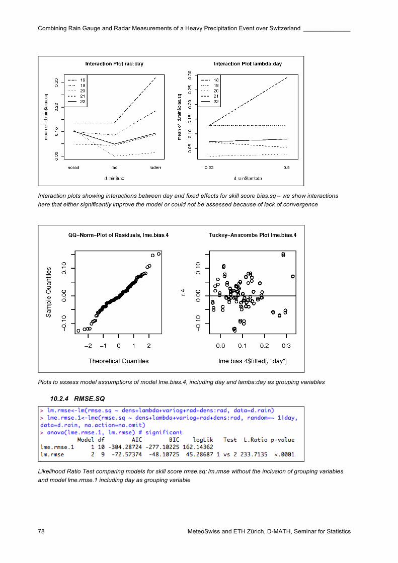
Combining Rain Gauge and Radar Measurements of a Heavy Precipitation Event over Switzerland ______________
MeteoSwiss and ETH Zürich, D-MATH, Seminar for Statistics 78
Interaction plots showing interactions between day and fixed effects for skill score bias.sq – we show interactions
here that either significantly improve the model or could not be assessed because of lack of convergence
Plots to assess model assumptions of model lme.bias.4, including day and lamba:day as grouping variables
10.2.4 RMSE.SQ
Likelihood Ratio Test comparing models for skill score rmse.sq: lm.rmse without the inclusion of grouping variables
and model lme.rmse.1 including day as grouping variable
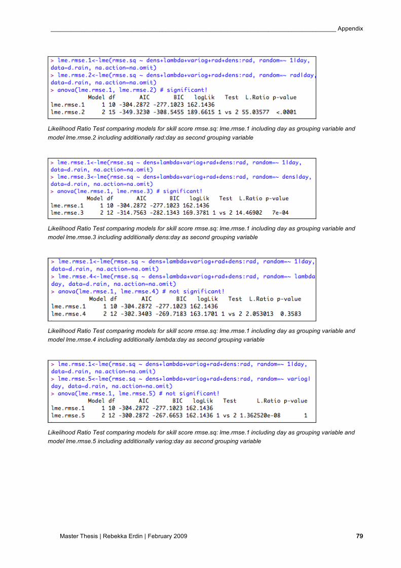
____________________________________________________________________________________ Appendix
Master Thesis | Rebekka Erdin | February 2009 79 79
Likelihood Ratio Test comparing models for skill score rmse.sq: lme.rmse.1 including day as grouping variable and
model lme.rmse.2 including additionally rad:day as second grouping variable
Likelihood Ratio Test comparing models for skill score rmse.sq: lme.rmse.1 including day as grouping variable and
model lme.rmse.3 including additionally dens:day as second grouping variable
Likelihood Ratio Test comparing models for skill score rmse.sq: lme.rmse.1 including day as grouping variable and
model lme.rmse.4 including additionally lambda:day as second grouping variable
Likelihood Ratio Test comparing models for skill score rmse.sq: lme.rmse.1 including day as grouping variable and
model lme.rmse.5 including additionally variog:day as second grouping variable
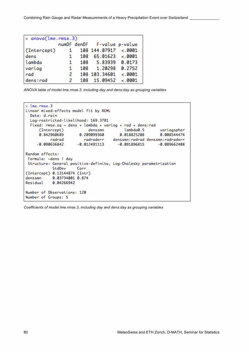
Combining Rain Gauge and Radar Measurements of a Heavy Precipitation Event over Switzerland ______________
MeteoSwiss and ETH Zürich, D-MATH, Seminar for Statistics 80
ANOVA table of model lme.rmse.3, including day and dens:day as grouping variables
Coefficients of model lme.rmse.3, including day and dens:day as grouping variables
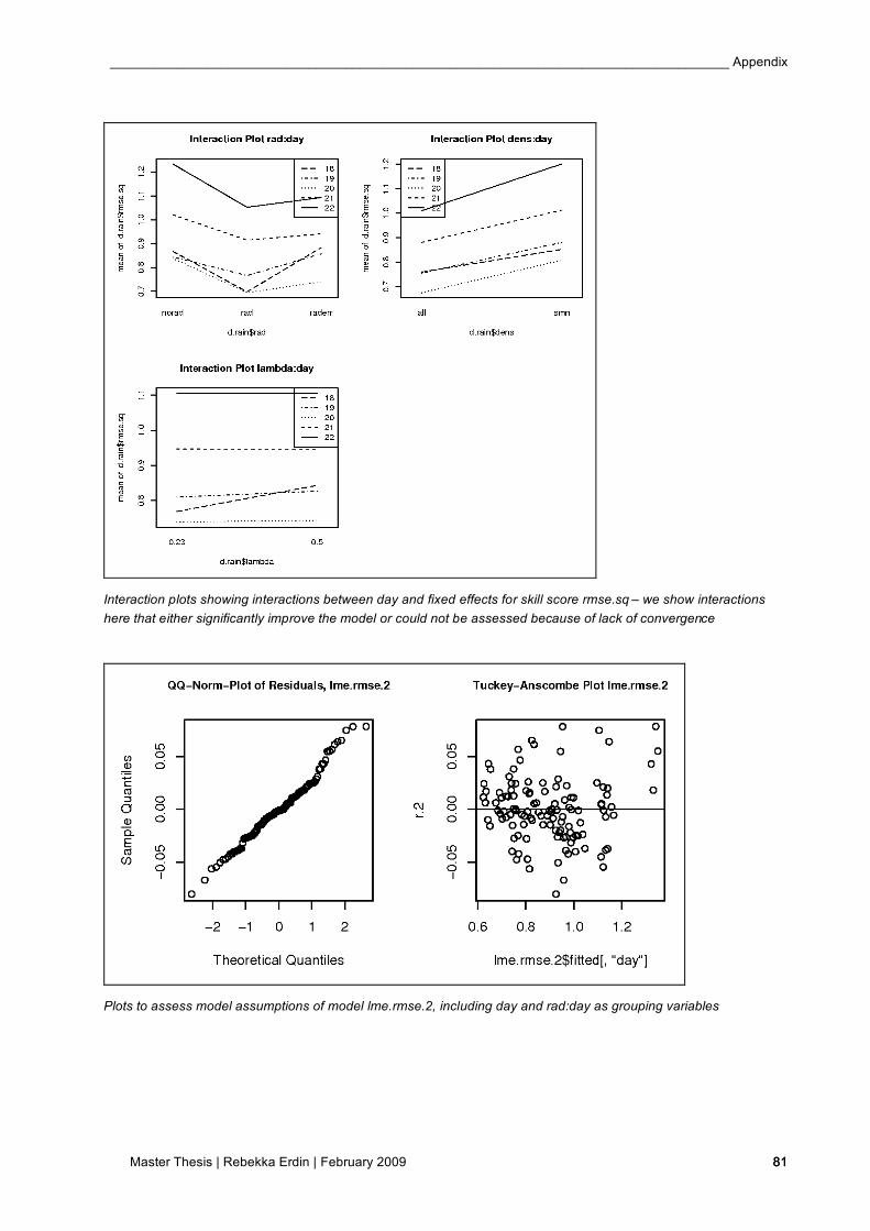
____________________________________________________________________________________ Appendix
Master Thesis | Rebekka Erdin | February 2009 81 81
Interaction plots showing interactions between day and fixed effects for skill score rmse.sq – we show interactions
here that either significantly improve the model or could not be assessed because of lack of convergence
Plots to assess model assumptions of model lme.rmse.2, including day and rad:day as grouping variables
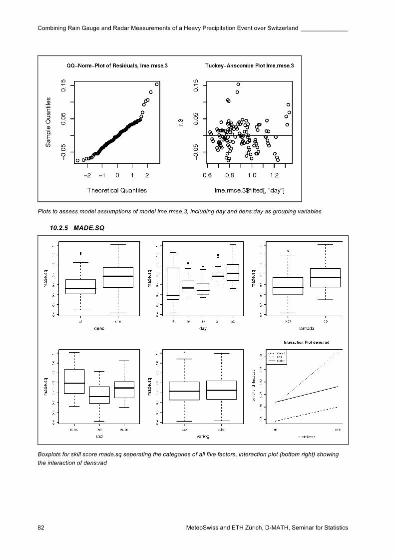
Combining Rain Gauge and Radar Measurements of a Heavy Precipitation Event over Switzerland ______________
MeteoSwiss and ETH Zürich, D-MATH, Seminar for Statistics 82
Plots to assess model assumptions of model lme.rmse.3, including day and dens:day as grouping variables
10.2.5 MADE.SQ
Boxplots for skill score made.sq seperating the categories of all five factors, interaction plot (bottom right) showing
the interaction of dens:rad
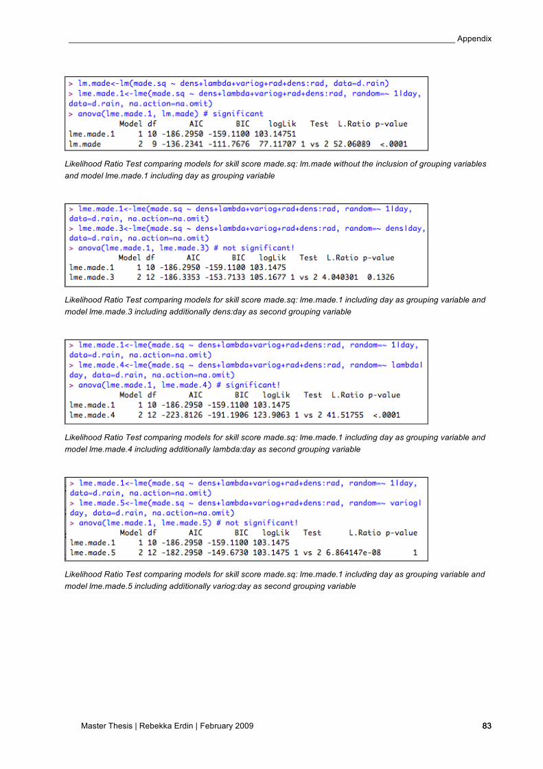
____________________________________________________________________________________ Appendix
Master Thesis | Rebekka Erdin | February 2009 83 83
Likelihood Ratio Test comparing models for skill score made.sq: lm.made without the inclusion of grouping variables
and model lme.made.1 including day as grouping variable
Likelihood Ratio Test comparing models for skill score made.sq: lme.made.1 including day as grouping variable and
model lme.made.3 including additionally dens:day as second grouping variable
Likelihood Ratio Test comparing models for skill score made.sq: lme.made.1 including day as grouping variable and
model lme.made.4 including additionally lambda:day as second grouping variable
Likelihood Ratio Test comparing models for skill score made.sq: lme.made.1 including day as grouping variable and
model lme.made.5 including additionally variog:day as second grouping variable
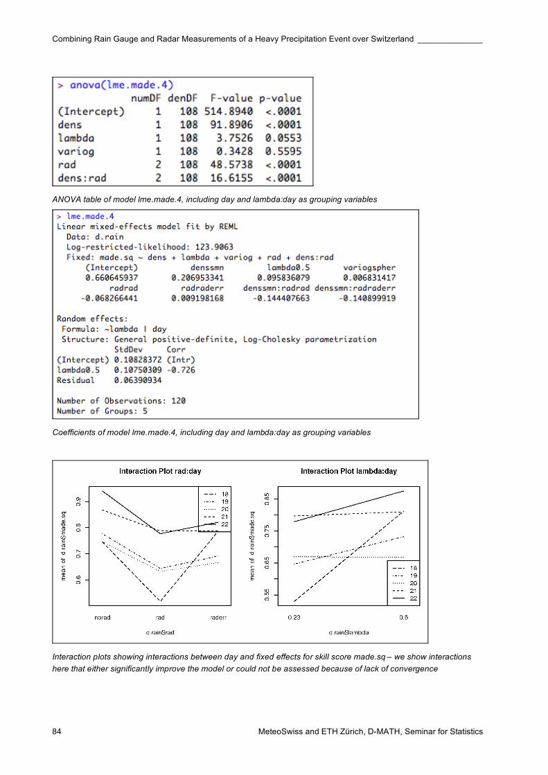
Combining Rain Gauge and Radar Measurements of a Heavy Precipitation Event over Switzerland ______________
MeteoSwiss and ETH Zürich, D-MATH, Seminar for Statistics 84
ANOVA table of model lme.made.4, including day and lambda:day as grouping variables
Coefficients of model lme.made.4, including day and lambda:day as grouping variables
Interaction plots showing interactions between day and fixed effects for skill score made.sq – we show interactions
here that either significantly improve the model or could not be assessed because of lack of convergence
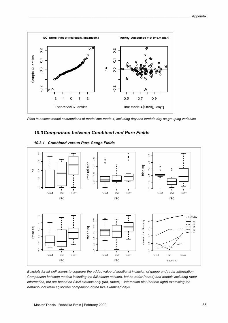
____________________________________________________________________________________ Appendix
Master Thesis | Rebekka Erdin | February 2009 85 85
Plots to assess model assumptions of model lme.made.4, including day and lambda:day as grouping variables
10.3 Comparison between Combined and Pure Fields
10.3.1 Combined versus Pure Gauge Fields
Boxplots for all skill scores to compare the added value of additional inclusion of gauge and radar information:
Comparison between models including the full station network, but no radar (norad) and models including radar
information, but are based on SMN stations only (rad, raderr) – interaction plot (bottom right) examining the
behaviour of rmse.sq for this comparison of the five examined days
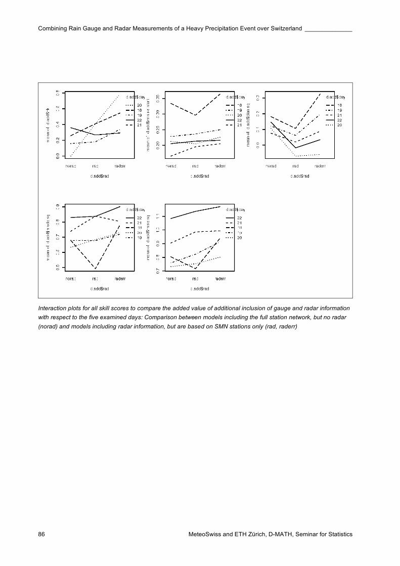
Combining Rain Gauge and Radar Measurements of a Heavy Precipitation Event over Switzerland ______________
MeteoSwiss and ETH Zürich, D-MATH, Seminar for Statistics 86
Interaction plots for all skill scores to compare the added value of additional inclusion of gauge and radar information
with respect to the five examined days: Comparison between models including the full station network, but no radar
(norad) and models including radar information, but are based on SMN stations only (rad, raderr)
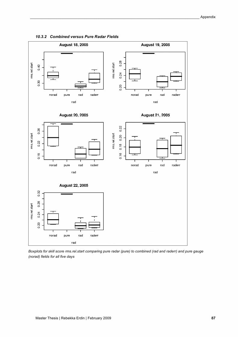
____________________________________________________________________________________ Appendix
Master Thesis | Rebekka Erdin | February 2009 87 87
10.3.2 Combined versus Pure Radar Fields
Boxplots for skill score rms.rel.start comparing pure radar (pure) to combined (rad and raderr) and pure gauge
(norad) fields for all five days
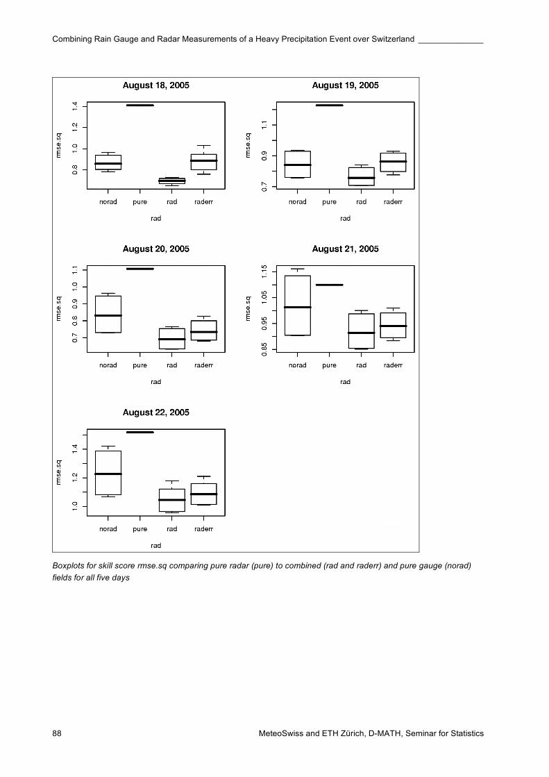
Combining Rain Gauge and Radar Measurements of a Heavy Precipitation Event over Switzerland ______________
MeteoSwiss and ETH Zürich, D-MATH, Seminar for Statistics 88
Boxplots for skill score rmse.sq comparing pure radar (pure) to combined (rad and raderr) and pure gauge (norad)
fields for all five days
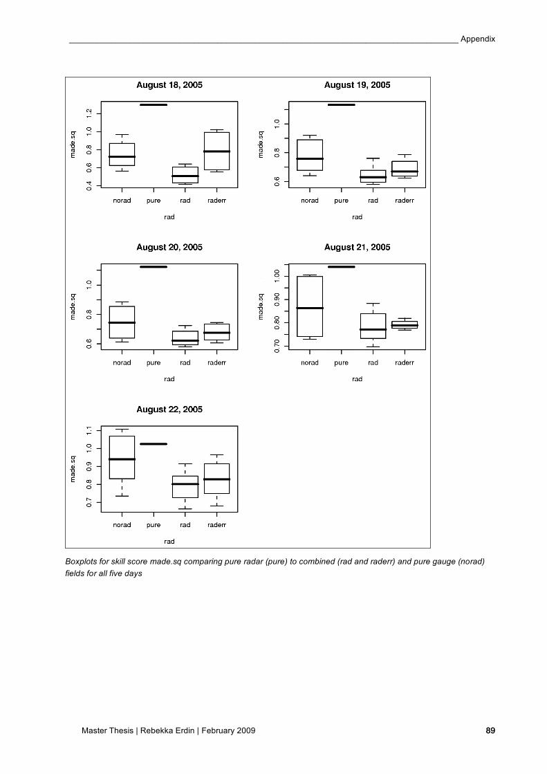
____________________________________________________________________________________ Appendix
Master Thesis | Rebekka Erdin | February 2009 89 89
Boxplots for skill score made.sq comparing pure radar (pure) to combined (rad and raderr) and pure gauge (norad)
fields for all five days
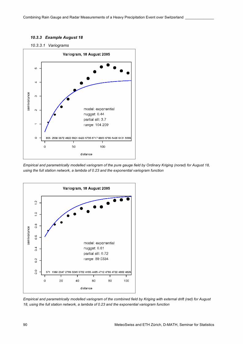
Combining Rain Gauge and Radar Measurements of a Heavy Precipitation Event over Switzerland ______________
MeteoSwiss and ETH Zürich, D-MATH, Seminar for Statistics 90
10.3.3 Example August 18
10.3.3.1 Variograms
Empirical and parametrically modelled variogram of the pure gauge field by Ordinary Kriging (norad) for August 18,
using the full station network, a lambda of 0.23 and the exponential variogram function
Empirical and parametrically modelled variogram of the combined field by Kriging with external drift (rad) for August
18, using the full station network, a lambda of 0.23 and the exponential variogram function
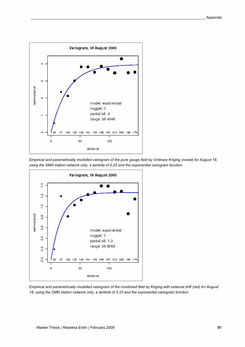
____________________________________________________________________________________ Appendix
Master Thesis | Rebekka Erdin | February 2009 91 91
Empirical and parametrically modelled variogram of the pure gauge field by Ordinary Kriging (norad) for August 18,
using the SMN station network only, a lambda of 0.23 and the exponential variogram function
Empirical and parametrically modelled variogram of the combined field by Kriging with external drift (rad) for August
18, using the SMN station network only, a lambda of 0.23 and the exponential variogram function

Combining Rain Gauge and Radar Measurements of a Heavy Precipitation Event over Switzerland ______________
MeteoSwiss and ETH Zürich, D-MATH, Seminar for Statistics 92
10.3.3.2 Plots Assessing Model Assumptions
Plots to assess model assumptions of the pure gauge field by Ordinary Kriging (norad) for August 18, using the full
station network, a lambda of 0.23 and the exponential variogram function
Plots to assess model assumptions of the combined field by Kriging with external drift (rad) for August 18, using the
full station network, a lambda of 0.23 and the exponential variogram function

____________________________________________________________________________________ Appendix
Master Thesis | Rebekka Erdin | February 2009 93 93
Plots to assess model assumptions of the pure gauge field by Ordinary Kriging (norad) for August 18, using the SMN
station network only, a lambda of 0.23 and the exponential variogram function
Plots to assess model assumptions of the combined field by Kriging with external drift (rad) for August 18, using the
SMN station network only, a lambda of 0.23 and the exponential variogram function
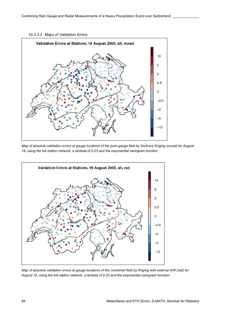
Combining Rain Gauge and Radar Measurements of a Heavy Precipitation Event over Switzerland ______________
MeteoSwiss and ETH Zürich, D-MATH, Seminar for Statistics 94
10.3.3.3 Maps of Validation Errors
Map of absolute validation errors at gauge locations of the pure gauge field by Ordinary Kriging (norad) for August
18, using the full station network, a lambda of 0.23 and the exponential variogram function
Map of absolute validation errors at gauge locations of the combined field by Kriging with external drift (rad) for
August 18, using the full station network, a lambda of 0.23 and the exponential variogram function
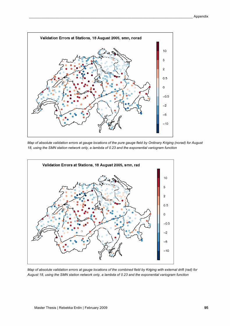
____________________________________________________________________________________ Appendix
Master Thesis | Rebekka Erdin | February 2009 95 95
Map of absolute validation errors at gauge locations of the pure gauge field by Ordinary Kriging (norad) for August
18, using the SMN station network only, a lambda of 0.23 and the exponential variogram function
Map of absolute validation errors at gauge locations of the combined field by Kriging with external drift (rad) for
August 18, using the SMN station network only, a lambda of 0.23 and the exponential variogram function
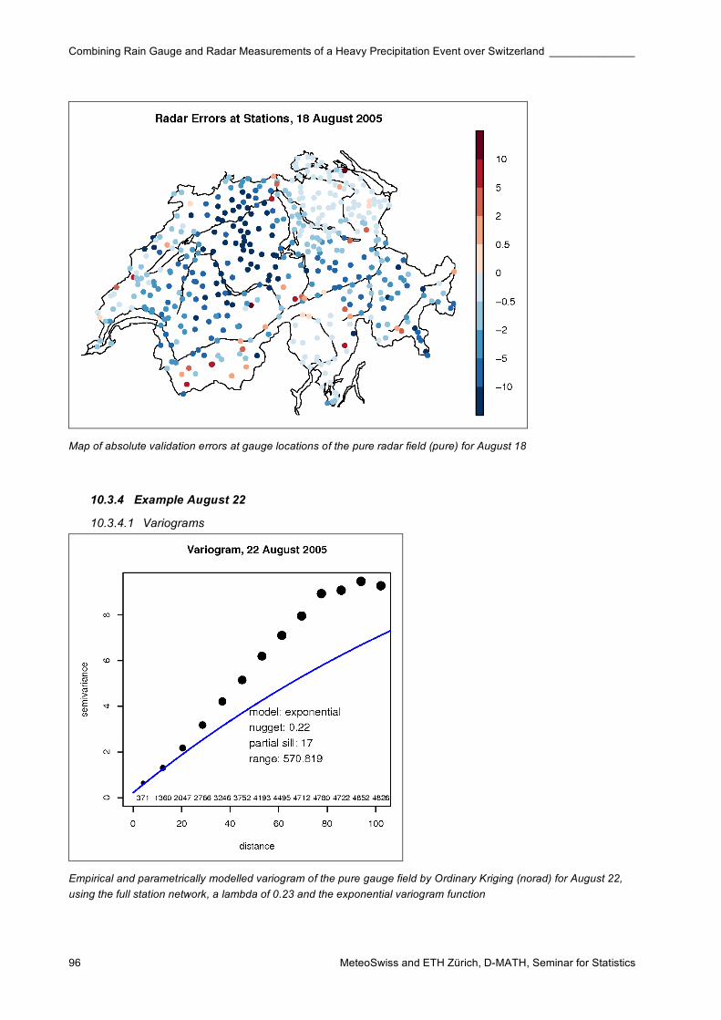
Combining Rain Gauge and Radar Measurements of a Heavy Precipitation Event over Switzerland ______________
MeteoSwiss and ETH Zürich, D-MATH, Seminar for Statistics 96
Map of absolute validation errors at gauge locations of the pure radar field (pure) for August 18
10.3.4 Example August 22
10.3.4.1 Variograms
Empirical and parametrically modelled variogram of the pure gauge field by Ordinary Kriging (norad) for August 22,
using the full station network, a lambda of 0.23 and the exponential variogram function
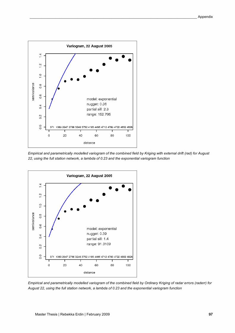
____________________________________________________________________________________ Appendix
Master Thesis | Rebekka Erdin | February 2009 97 97
Empirical and parametrically modelled variogram of the combined field by Kriging with external drift (rad) for August
22, using the full station network, a lambda of 0.23 and the exponential variogram function
Empirical and parametrically modelled variogram of the combined field by Ordinary Kriging of radar errors (raderr) for
August 22, using the full station network, a lambda of 0.23 and the exponential variogram function
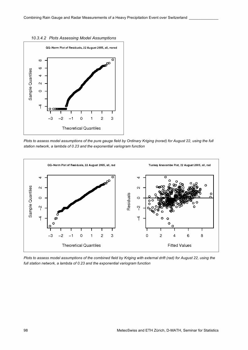
Combining Rain Gauge and Radar Measurements of a Heavy Precipitation Event over Switzerland ______________
MeteoSwiss and ETH Zürich, D-MATH, Seminar for Statistics 98
10.3.4.2 Plots Assessing Model Assumptions
Plots to assess model assumptions of the pure gauge field by Ordinary Kriging (norad) for August 22, using the full
station network, a lambda of 0.23 and the exponential variogram function
Plots to assess model assumptions of the combined field by Kriging with external drift (rad) for August 22, using the
full station network, a lambda of 0.23 and the exponential variogram function

____________________________________________________________________________________ Appendix
Master Thesis | Rebekka Erdin | February 2009 99 99
Plots to assess model assumptions of the combined field by Ordinary Kriging of radar errors (raderr) for August 22,
using the full station network, a lambda of 0.23 and the exponential variogram function
10.3.4.3 Predicted fields
Predicted field by pure radar field (pure) for August 22, compared to measured values at gauge locations (dots)
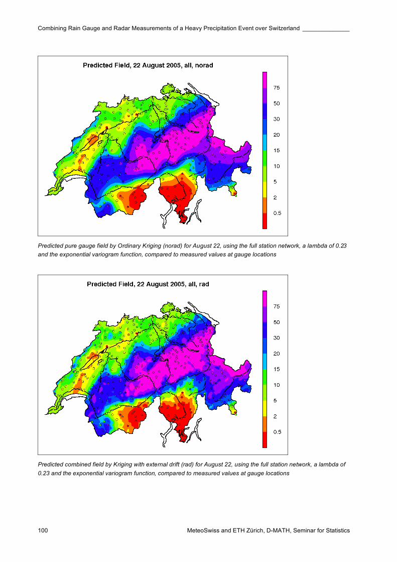
Combining Rain Gauge and Radar Measurements of a Heavy Precipitation Event over Switzerland ______________
MeteoSwiss and ETH Zürich, D-MATH, Seminar for Statistics 100
Predicted pure gauge field by Ordinary Kriging (norad) for August 22, using the full station network, a lambda of 0.23
and the exponential variogram function, compared to measured values at gauge locations
Predicted combined field by Kriging with external drift (rad) for August 22, using the full station network, a lambda of
0.23 and the exponential variogram function, compared to measured values at gauge locations
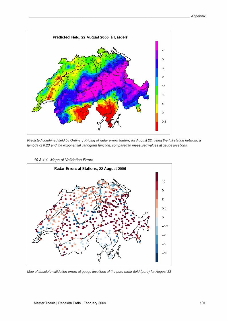
____________________________________________________________________________________ Appendix
Master Thesis | Rebekka Erdin | February 2009 101 101
Predicted combined field by Ordinary Kriging of radar errors (raderr) for August 22, using the full station network, a
lambda of 0.23 and the exponential variogram function, compared to measured values at gauge locations
10.3.4.4 Maps of Validation Errors
Map of absolute validation errors at gauge locations of the pure radar field (pure) for August 22
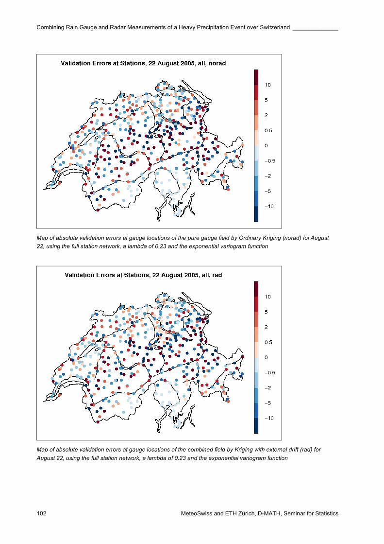
Combining Rain Gauge and Radar Measurements of a Heavy Precipitation Event over Switzerland ______________
MeteoSwiss and ETH Zürich, D-MATH, Seminar for Statistics 102
Map of absolute validation errors at gauge locations of the pure gauge field by Ordinary Kriging (norad) for August
22, using the full station network, a lambda of 0.23 and the exponential variogram function
Map of absolute validation errors at gauge locations of the combined field by Kriging with external drift (rad) for
August 22, using the full station network, a lambda of 0.23 and the exponential variogram function
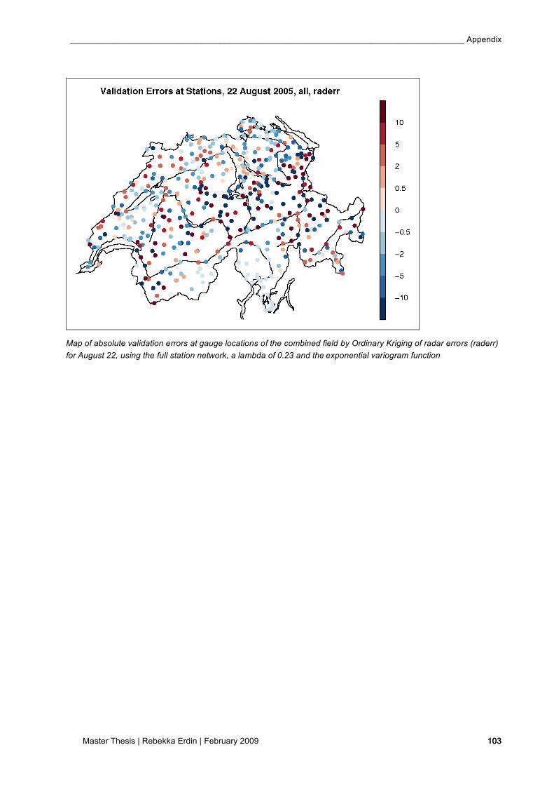
____________________________________________________________________________________ Appendix
Master Thesis | Rebekka Erdin | February 2009 103 103
Map of absolute validation errors at gauge locations of the combined field by Ordinary Kriging of radar errors (raderr)
for August 22, using the full station network, a lambda of 0.23 and the exponential variogram function
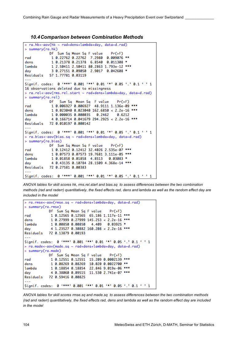
Combining Rain Gauge and Radar Measurements of a Heavy Precipitation Event over Switzerland ______________
MeteoSwiss and ETH Zürich, D-MATH, Seminar for Statistics 104
10.4 Comparison between Combination Methods
ANOVA tables for skill scores hk, rms.rel.start and bias.sq to assess differences between the two combination
methods (rad and raderr) quantitatively, the fixed effects rad, dens and lambda as well as the random effect day are
included in the model
ANOVA tables for skill scores rmse.sq and made.sq to assess differences between the two combination methods
(rad and raderr) quantitatively, the fixed effects rad, dens and lambda as well as the random effect day are included
in the model
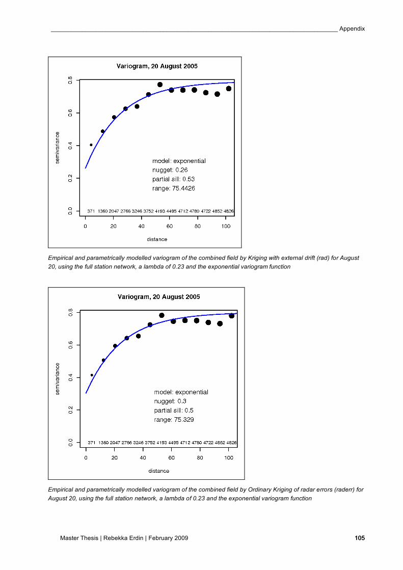
____________________________________________________________________________________ Appendix
Master Thesis | Rebekka Erdin | February 2009 105 105
Empirical and parametrically modelled variogram of the combined field by Kriging with external drift (rad) for August
20, using the full station network, a lambda of 0.23 and the exponential variogram function
Empirical and parametrically modelled variogram of the combined field by Ordinary Kriging of radar errors (raderr) for
August 20, using the full station network, a lambda of 0.23 and the exponential variogram function
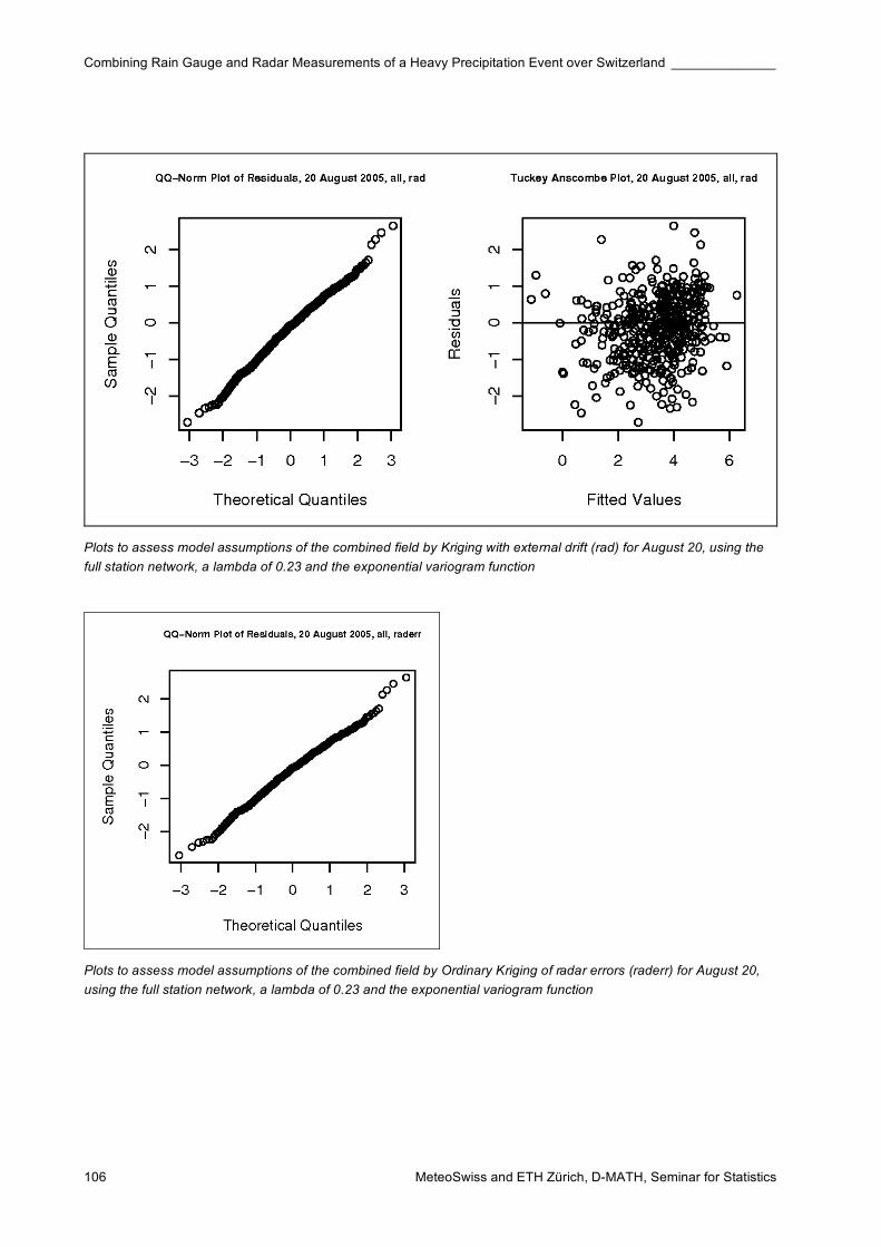
Combining Rain Gauge and Radar Measurements of a Heavy Precipitation Event over Switzerland ______________
MeteoSwiss and ETH Zürich, D-MATH, Seminar for Statistics 106
Plots to assess model assumptions of the combined field by Kriging with external drift (rad) for August 20, using the
full station network, a lambda of 0.23 and the exponential variogram function
Plots to assess model assumptions of the combined field by Ordinary Kriging of radar errors (raderr) for August 20,
using the full station network, a lambda of 0.23 and the exponential variogram function
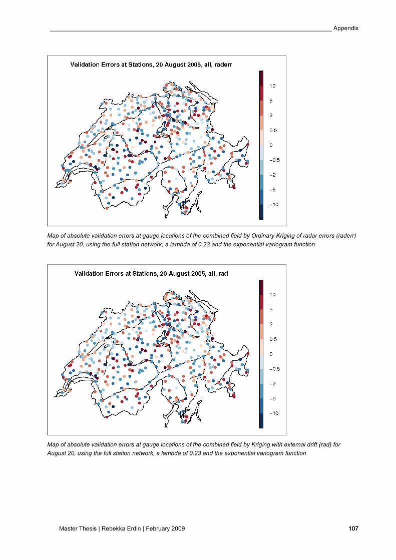
____________________________________________________________________________________ Appendix
Master Thesis | Rebekka Erdin | February 2009 107 107
Map of absolute validation errors at gauge locations of the combined field by Ordinary Kriging of radar errors (raderr)
for August 20, using the full station network, a lambda of 0.23 and the exponential variogram function
Map of absolute validation errors at gauge locations of the combined field by Kriging with external drift (rad) for
August 20, using the full station network, a lambda of 0.23 and the exponential variogram function
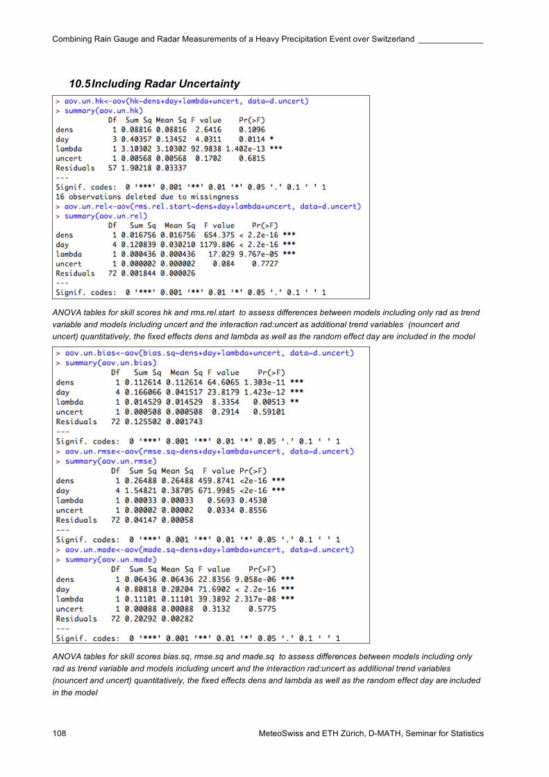
Combining Rain Gauge and Radar Measurements of a Heavy Precipitation Event over Switzerland ______________
MeteoSwiss and ETH Zürich, D-MATH, Seminar for Statistics 108
10.5 Including Radar Uncertainty
ANOVA tables for skill scores hk and rms.rel.start to assess differences between models including only rad as trend
variable and models including uncert and the interaction rad:uncert as additional trend variables (nouncert and
uncert) quantitatively, the fixed effects dens and lambda as well as the random effect day are included in the model
ANOVA tables for skill scores bias.sq, rmse.sq and made.sq to assess differences between models including only
rad as trend variable and models including uncert and the interaction rad:uncert as additional trend variables
(nouncert and uncert) quantitatively, the fixed effects dens and lambda as well as the random effect day are included
in the model

Kürzlich erschienen
Frühere Veröffentlichungen und Arbeitsberichte finden sich unter
72 Mathis H: 2005, Impact of Realistic Greenhouse Gas Forcing on Seasonal Forecast Performance, 80pp, CHF 75.-
www.meteoschweiz.ch » Forschung » Publikationen
Veröffentlichungen der MeteoSchweiz 80 Buzzi M: 2009, Challenges in Operational Numerical Weather Prediction at High Resolution in
Complex Terrain, 204 pp, CHF 103.-
79 Nowak D: 2008, Radiation and clouds: observations and model calculations for Payerne BSRN site, 101 pp, CHF 80.-
78 Arpagaus M, Rotach M, Ambrosetti P, Ament F, Appenzeller C, Bauer H-S, Bouttier F, Buzzi A, Corazza M, Davolio S, Denhard M, Dorninger M, Fontannaz L, Frick J, Fundel F, Germann U, Gorgas T, Grossi G, Hegg C, Hering A, Jaun S, Keil C, Liniger M, Marsigli C, McTaggart-Cowan R, Montani A, Mylne K, Ranzi R, Richard E, Rossa A, Santos-Muñoz D, Schär C, Seity Y, Staudinger M, Stoll M, Vogt S, Volkert H, Walser A, Wang Y, Werhahn J, Wulfmeyer V, Wunram C and Zappa M: 2009, MAP D-PHASE: Demonstrating forecast capabilities for flood events in the Alpine region. Report of the WWRP Forecast Demonstration Project D-PHASE submitted to the WWRP Scientific Steering Committee, 65pp, CHF 73.-
77 Rossa AM: 2007, MAP-NWS – an Optional EUMETNET Programme in Support of an Optimal Research Programme, 67pp, CHF 73.-
76 Baggenstos D: 2007, Probabilistic verification of operational monthly temperature forecasts, 52pp, CHF 69.-
75 Fikke S, Ronsten G, Heimo A, Kunz S, Ostrozlik M, Persson PE, Sabata J, Wareing B, Wichura B, Chum J, Laakso T, Säntti K and Makkonen L: 2007, COST 727: Atmospheric Icing on Structures Measurements and data collection on icing: State of the Art, 110pp, CHF 83.-
74 Schmutz C, Müller P und Barodte B: 2006, Potenzialabklärung für Public Private Partnership (PPP) bei MeteoSchweiz und armasuisse Immobilien, 82pp, CHF 76.-
73 Scherrer SC: 2006, Interannual climate variability in the European and Alpine region, 132pp, CHF 86.-
71 Leuenberger D: 2005, High-Resolution Radar Rainfall Assimilation: Exploratory Studies with Latent Heat Nudging, 103pp, CHF 81.-
70 Müller G und Viatte P: 2005, The Swiss Contribution to the Global Atmosphere Watch Programme – Achievements of the First Decade and Future Prospects, 112pp, CHF 83.-
69 Müller WA: 2004, Analysis and Prediction of the European Winter Climate, 115pp, CHF 34.
68 Bader S: 2004, Das Schweizer Klima im Trend: Temperatur- und Niederschlagsentwicklung seit 1864, 48pp, CHF 18.-
67 Begert M, Seiz G, Schlegel T, Musa M, Baudraz G und Moesch M: 2003, Homogenisierung von Klimamessreihen der Schweiz und Bestimmung der Normwerte 1961-1990, Schluss-bericht des Projektes NORM90, 170pp, CHF 40.-
66 Schär C, Binder P and Richner H (Eds.): 2003, International Conference on Alpine Meteorology and MAP Meeting 2003, Extended Abstracts volumes A and B, 580pp, CHF 100.
65 Stübi R: 2002, SONDEX / OZEX campaigns of dual ozone sondes flights: Report on the data analysis, 78pp, CHF 27.-
64 Bolliger M: 2002, On the characteristics of heavy precipitation systems observed by Meteosat-6 during the MAP-SOP, 116pp, CHF 36.-
63 Favaro G, Jeannet P and Stübi R: 2002, Re-evaluation and trend analysis of the Payerne ozone sounding, 99pp, CHF 33.-

Kürzlich erschienen
Frühere Veröffentlichungen und Arbeitsberichte finden sich unter www.meteoschweiz.ch » Forschung » Publikationen
62 Bettems JM: 2001, EUCOS impact study using the limited-area non-hydrostatic NWP model in operational use at MeteoSwiss, 17pp, CHF 12.-
61 Richner H et al.: 1999, Grundlagen aerologischer Messungen speziell mittels der Schweizer Sonde SRS 400, 140pp, CHF 42.-
60 Gisler O: 1999, Zur Methodik einer Beschreibung der Entwicklung des linearen Trends der Lufttemperatur über der Schweiz im Zeitabschnitt von 1864 bis 1990, 125pp, CHF 36.-
59 Bettems J-M: 1999, The impact of hypothetical wind profiler networks on numerical weather prediction in the Alpine region, 65pp, CHF 25.-
58 Baudenbacher, M: 1997, Homogenisierung langer Klimareihen, dargelegt am Beispiel der Lufttemperatur, 181pp, CHF 50.-
57 Bosshard, W: 1996, Homogenisierung klimatologischer Zeitreihen, dargelegt am Beispiel der relativen Sonnenscheindauer, 136pp, CHF 38.-
Kürzlich erschienen
Frühere Veröffentlichungen und Arbeitsberichte finden sich unter www.meteoschweiz.ch » Forschung » Publikationen
Arbeitsberichte der MeteoSchweiz 226 MeteoSchweiz: 2009, Analysen der sicherheitsrelevanten klimatologischen Parameter am
Standort KKW-Mühleberg, 135pp, CHF 88.-
225 MeteoSchweiz: 2009, Analysen der sicherheitsrelevanten klimatologischen Parameter am Standort KKW-Gösgen, 135pp, CHF 88.-
224 MeteoSchweiz: 2009, Analysen der sicherheitsrelevanten klimatologischen Parameter am Standort KKW-Beznau, 135pp, CHF 88.-
223 Dürr B: 2008, Automatisiertes Verfahren zur Bestimmung von Föhn in den Alpentälern, 22pp, CHF 62.-
222 Schmutz C, Arpagaus M, Clementi L, Frei C, Fukutome S, Germann U, Liniger M und Schacher F: 2008, Meteorologische Ereignisanalyse des Hochwassers 8. bis 9. August 2007, 29pp, CHF 64.-
221 Frei C, Germann U, Fukutome S und Liniger M: 2008, Möglichkeiten und Grenzen der Niederschlagsanalysen zum Hochwasser 2005, 19pp, CHF 62.-
220 Ambühl J: 2008, Optimization of Warning Systems based on Economic Criteria, 79pp, CHF 75.-
219 Ceppi P, Della-Marta PM and Appenzeller C: 2008, Extreme Value Analysis of Wind Observations over Switzerland, 43pp, CHF 67.-
218 MeteoSchweiz (Hrsg): 2008, Klimaszenarien für die Schweiz – Ein Statusbericht, 50pp, CHF 69.-
217 Begert M: 2008, Die Repräsentativität der Stationen im Swiss National Basic Climatological Network (Swiss NBCN), 40pp, CHF 66.-
216 Della-Marta PM, Mathis H, Frei C, Liniger MA and Appenzeller C: 2007, Extreme wind storms over Europe: Statistical Analyses of ERA-40, 80pp, CHF 75.-
215 Begert M, Seiz G, Foppa N, Schlegel T, Appenzeller C und Müller G: 2007, Die Überführung der klimatologischen Referenzstationen der Schweiz in das Swiss National Climatological Network (Swiss NBCN), 47pp, CHF 68.-
214 Schmucki D und Weigel A: 2006, Saisonale Vorhersage in Tradition und Moderne: Vergleich der "Sommerprognose" des Zürcher Bööggs mit einem dynamischen Klimamodell, 46pp, CHF 68.-
213 Frei C: 2006, Eine Länder übergreifende Niederschlagsanalyse zum August Hochwasser 2005. Ergänzung zu Arbeitsbericht 211, 10pp, CHF 59.-
212 Z’graggen, L: 2006, Die Maximaltemperaturen im Hitzesommer 2003 und Vergleich zu früheren Extremtemperaturen, 74pp, CHF 75.-
211 MeteoSchweiz: 2006, Starkniederschlagsereignis August 2005, 63pp, CHF 72.-
210 Buss S, Jäger E and Schmutz C: 2005: Evaluation of turbulence forecasts with the aLMo, 58pp, CHF 70.–
209 Schmutz C, Schmuki D, Duding O, Rohling S: 2004, Aeronautical Climatological Information Sion LSGS, 77pp, CHF 25.–
208 Schmuki D, Schmutz C, Rohling S: 2004, Aeronautical Climatological Information Grenchen LSZG, 73pp, CHF 24.–
207 Moesch M, Zelenka A: 2004, Globalstrahlungsmessungen 1981-2000 im ANETZ, 83pp, CHF 26.–
206 Schmutz C, Schmuki D, Rohling S: 2004, Aeronautical Climatological Information St.Gallen LSZR, 78pp, CHF 25.–
Kürzlich erschienen
Frühere Veröffentlichungen und Arbeitsberichte finden sich unter www.meteoschweiz.ch » Forschung » Publikationen
205 Schmutz C, Schmuki D, Ambrosetti P, Gaia M, Rohling S: 2004, Aeronautical Climatological Information Lugano LSZA, 81pp, CHF 26.–
204 Schmuki D, Schmutz C, Rohling S: 2004, Aeronautical Climatological Information Bern LSZB, 80pp, CHF 25.–
203 Duding O, Schmuki D, Schmutz C, Rohling S: 2004, Aeronautical Climatological Information Geneva LSGG, 104pp, CHF 31.–
202 Bader S: 2004, Tropische Wirbelstürme – Hurricanes –Typhoons – Cyclones, 40pp, CHF 16.-
201 Schmutz C, Schmuki D, Rohling S: 2004, Aeronautical Climatological Information Zurich LSZH, 110pp, CHF 34.-
200 Bader S: 2004, Die extreme Sommerhitze im aussergewöhnlichen Witterungsjahr 2003, 25pp, CHF 14.-