combustion analysis for flame stability predictions at ... · abstract combustion analysis for...

Combustion Analysis For Flame Stability Predictions atGround Level and Altitude in Aviation Gas Turbine Engines

with Low Emissions Combustors

by

Tomas Turek

A thesis submitted in conformity with the requirementsfor the degree of Master of Applied Science

Graduate Department of Aerospace Science and EngineeringUniversity of Toronto

© Copyright 2015 by Tomas Turek

Abstract

Combustion Analysis For Flame Stability Predictions at Ground Leveland Altitude in Aviation Gas Turbine Engines with Low Emissions

Combustors

Tomas Turek

Master of Applied Science

Graduate Department of Aerospace Science and Engineering

University of Toronto

2015

Low emissions combustors operating with low fuel/air ratios may have challenges with flame

stability. As combustion is made leaner in the primary zone, the flame can lose its stability,

resulting in operability problems such as relight, flameout or cold starting. This thesis analyzes

combustion processes for the prediction on flame stability in low emissions combustors.

A detailed review of the literature on flame stability was conducted and main approaches in

flame stability modelling were indicated. Three flame stability models were proposed (Char-

acteristic Time, Loading Parameter, and Combustion Efficiency models) and developed into a

unique Preliminary Multi-Disciplinary Design Optimization (PMDO) tool. Results were val-

idated with a database of experimental combustor test data and showed that flame stability

can be predicted for an arbitrary shape of combustors running at any operational conditions

including ground and altitude situations with various jet fuels and nozzles. In conclusion, flame

stability can be predicted for newly designed low emission combustors.

ii

Acknowledgements

I would like to express my sincere gratitude and appreciation to my supervisor, Prof. Sam

Sampath, for his excellent technical lead of this thesis. Also, I am thankful for his willingness

to help me with any of concerns I had throughout my studies. I would like to acknowledge the

director of UTIAS, Prof. David W. Zingg, and associate director of UTIAS, Prof. Hugh H.T.

Liu, for their attentiveness and efforts during our consultations to direct my studies in the right

way. Furthermore, I would like to express my sincerest thanks to a Canadian aircraft engine

manufacturer, Pratt & Whitney Canada, for providing crucial experimental data of combustors

necessary for this research.

Most importantly, I own my deepest gratitude to my parents and brother for their patience

and accommodation throughout my studies. I would like to extend my heartfelt appreciation

to my girlfriend, Shuyi, for her assistance and encouragement in finishing my studies. Without

them, it will certainly not be possible to complete this thesis.

iii

“Everything we hear is an opinion, not a fact.

Everything we see is a perspective, not the truth.”

− Marcus Aurelius, Meditations

“To understand the true quality of people, you must look into their minds, and examine their

pursuits and aversions.”

− Marcus Aurelius, Meditations

v

Contents

List of Tables ix

List of Figures xi

List of Symbols xv

1 Introduction 1

1.1 Gas Turbine Combustors . . . . . . . . . . . . . . . . . . . . . . . . . . . . . . . . 3

1.2 Flame Stability in Gas Turbines . . . . . . . . . . . . . . . . . . . . . . . . . . . 5

1.2.1 Ignition in Gas Turbines Following Flame Instability . . . . . . . . . . . . 8

1.2.2 Role of Transient Performance of Gas Turbines in Flame Stability . . . . 9

1.3 Combustion Analysis for Preliminary Design . . . . . . . . . . . . . . . . . . . . 10

1.4 Goal of Thesis . . . . . . . . . . . . . . . . . . . . . . . . . . . . . . . . . . . . . 15

2 Flame Stability 17

2.1 Flame Extinction . . . . . . . . . . . . . . . . . . . . . . . . . . . . . . . . . . . . 18

2.1.1 Flame Stretch . . . . . . . . . . . . . . . . . . . . . . . . . . . . . . . . . . 18

2.1.2 Edge Flame Structures . . . . . . . . . . . . . . . . . . . . . . . . . . . . . 20

2.2 Flame Stabilization . . . . . . . . . . . . . . . . . . . . . . . . . . . . . . . . . . . 23

2.2.1 Stabilization and Blowoff Mechanisms of Premixed Flames . . . . . . . . 23

2.2.2 Blowout Mechanisms of Non-Premixed Flames . . . . . . . . . . . . . . . 25

2.3 Flow Characteristics Near Lean Blowout Limits in Model Combustors . . . . . . 27

3 Flame Stability Modelling 29

3.1 Semi-Empirical Analytical Models for Flame Stability . . . . . . . . . . . . . . . 29

3.1.1 Characteristic Time Models . . . . . . . . . . . . . . . . . . . . . . . . . . 30

3.1.2 Loading Parameter Models . . . . . . . . . . . . . . . . . . . . . . . . . . 33

3.1.3 Other Models . . . . . . . . . . . . . . . . . . . . . . . . . . . . . . . . . . 37

3.2 Numerical Modelling of Flame Stablity . . . . . . . . . . . . . . . . . . . . . . . . 37

4 Test Cases of Thesis Combustors 41

vii

4.1 Combustors . . . . . . . . . . . . . . . . . . . . . . . . . . . . . . . . . . . . . . . 41

4.1.1 Combustor A . . . . . . . . . . . . . . . . . . . . . . . . . . . . . . . . . . 41

4.1.2 Combustor B . . . . . . . . . . . . . . . . . . . . . . . . . . . . . . . . . . 43

4.1.3 Combustor C . . . . . . . . . . . . . . . . . . . . . . . . . . . . . . . . . . 43

4.2 Fuels . . . . . . . . . . . . . . . . . . . . . . . . . . . . . . . . . . . . . . . . . . . 44

4.2.1 Fuel Atomization . . . . . . . . . . . . . . . . . . . . . . . . . . . . . . . . 44

4.2.2 Fuel Evaporation . . . . . . . . . . . . . . . . . . . . . . . . . . . . . . . . 47

4.3 Experimental Tests . . . . . . . . . . . . . . . . . . . . . . . . . . . . . . . . . . . 49

5 Developed PMDO Tool for Flame Stability Predictions 51

5.1 Flame Stability Model . . . . . . . . . . . . . . . . . . . . . . . . . . . . . . . . . 51

5.2 Characteristics of Models Employed in FSM . . . . . . . . . . . . . . . . . . . . . 53

5.2.1 CTM . . . . . . . . . . . . . . . . . . . . . . . . . . . . . . . . . . . . . . 53

5.2.2 LPM . . . . . . . . . . . . . . . . . . . . . . . . . . . . . . . . . . . . . . . 55

5.2.3 CEM . . . . . . . . . . . . . . . . . . . . . . . . . . . . . . . . . . . . . . . 56

5.3 Predictions at Ground Level and Altitude . . . . . . . . . . . . . . . . . . . . . . 58

5.4 Accuracy and Limitations of FSM . . . . . . . . . . . . . . . . . . . . . . . . . . 59

6 Results of FSM 61

6.0.1 Combustor A . . . . . . . . . . . . . . . . . . . . . . . . . . . . . . . . . . 62

6.0.2 Combustor B . . . . . . . . . . . . . . . . . . . . . . . . . . . . . . . . . . 65

6.0.3 Combustor C . . . . . . . . . . . . . . . . . . . . . . . . . . . . . . . . . . 66

6.0.4 Global Correlation of Flame Stability Limit . . . . . . . . . . . . . . . . . 69

7 Conclusions 71

7.1 Future Work . . . . . . . . . . . . . . . . . . . . . . . . . . . . . . . . . . . . . . 73

Bibliography 75

Appendix A Results of FSM for Tested Combustors 85

A.1 Combustor A . . . . . . . . . . . . . . . . . . . . . . . . . . . . . . . . . . . . . . 86

A.2 Combustor B . . . . . . . . . . . . . . . . . . . . . . . . . . . . . . . . . . . . . . 88

A.3 Combustor C . . . . . . . . . . . . . . . . . . . . . . . . . . . . . . . . . . . . . . 90

viii

List of Tables

3.1 Values of A employed in Equation ?? for aircraft engines, [2]. . . . . . . . . . . . 35

4.1 Tested combustors. . . . . . . . . . . . . . . . . . . . . . . . . . . . . . . . . . . . 41

4.2 Tested nozzles. . . . . . . . . . . . . . . . . . . . . . . . . . . . . . . . . . . . . . 46

5.1 Interpretation of FSM results. . . . . . . . . . . . . . . . . . . . . . . . . . . . . . 52

6.1 Model constants. . . . . . . . . . . . . . . . . . . . . . . . . . . . . . . . . . . . . 61

A.1 FSM data – Combustor A, Data: Lean limit test, Pressure atomizer: Simplex

3.0 FN. . . . . . . . . . . . . . . . . . . . . . . . . . . . . . . . . . . . . . . . . . 86

A.2 FSM data – Combustor A, Data: Lean limit test, Pressure atomizer: Simplex

0.9 FN. . . . . . . . . . . . . . . . . . . . . . . . . . . . . . . . . . . . . . . . . . 87

A.3 FSM data – Combustor A, Data: Lean limit test, Airblast atomizer. . . . . . . . 87

A.4 FSM data – Combustor B, Data: Atmospheric test, Pressure atomizer: Simplex

2.25 FN. . . . . . . . . . . . . . . . . . . . . . . . . . . . . . . . . . . . . . . . . . 88

A.5 FSM data – Combustor B, Data: Atmospheric test, Airblast atomizer. . . . . . . 89

A.6 FSM data – Combustor C, Data: Atmospheric test, Pressure atomizer: Simplex

0.65 FN. . . . . . . . . . . . . . . . . . . . . . . . . . . . . . . . . . . . . . . . . . 90

A.7 FSM data – Combustor C, Data: Atmospheric test, Pressure atomizer: Simplex

1.1 FN. . . . . . . . . . . . . . . . . . . . . . . . . . . . . . . . . . . . . . . . . . 91

A.8 FSM data – Combustor C, Data: Gas generator test, Pressure atomizer: Simplex

1.9 FN. . . . . . . . . . . . . . . . . . . . . . . . . . . . . . . . . . . . . . . . . . 92

A.9 FSM data – Combustor C, Data: Gas generator test, Pressure atomizer: Simplex

2.2 FN. . . . . . . . . . . . . . . . . . . . . . . . . . . . . . . . . . . . . . . . . . 93

ix

List of Figures

1.1 Conventional combustors [2]: (a) Three main types of combustors, (b) Annular

combustor. . . . . . . . . . . . . . . . . . . . . . . . . . . . . . . . . . . . . . . . 3

1.2 Conventional aircraft combustor [2]: (a) Main components, (b) Typical primary-

zone configuration for an annular combustor. . . . . . . . . . . . . . . . . . . . . 5

1.3 Typical combustor characteristics (adapted from Lefebvre, [2]): (a) stability loop,

(b) ignition loop. . . . . . . . . . . . . . . . . . . . . . . . . . . . . . . . . . . . . 6

1.4 Aircraft combustor performance (adapted from Lefebvre, [2]): (a) stability per-

formance, (b) ignition performance. . . . . . . . . . . . . . . . . . . . . . . . . . . 7

1.5 Altitude charts [14]: (a) propulsive duct, (b) Mach number and intake air velocity

with altitude. . . . . . . . . . . . . . . . . . . . . . . . . . . . . . . . . . . . . . . 8

1.6 Combustor stability performance - influence of fuel injected state and fuel–air

unmixedness [15]. . . . . . . . . . . . . . . . . . . . . . . . . . . . . . . . . . . . . 8

1.7 Simple chemically reacting systems [20]: (a) constant–pressure, fixed mass; (b)

constant–volume, fixed mass; (c) well–stirred reactor; (d) plug-flow reactor. . . . 11

1.8 Reactor network for gas turbine can [21]. . . . . . . . . . . . . . . . . . . . . . . . 15

1.9 Reactor network simulating the quenching process for gas turbine [22]. . . . . . . 15

2.1 2D flames showing positive stretching of a flame surface by [25]: (a) tangential

velocity gradients along the flame, (b) motion of a curved flame (flame normal

is pointing into the products). . . . . . . . . . . . . . . . . . . . . . . . . . . . . . 19

2.2 Edged flames [31]: (a) flame spreading over a fuel-bed, (b) candle flame burning

under microgravity conditions, (c) wrinkled torn flame in turbulent flow, (d)

diffusion flame sitting on a plate through which fuel is injected. . . . . . . . . . . 21

2.3 Edge flame configurations [25]: (a) fuel/oxidizer interface with quasi-one-dimensional

non-premixed flame downstream, (b) premixed flame in shear layer with quasi-

one-dimensional premixed flame downstream, (c) ignition front, (d) flame holes

induced by local extinction. . . . . . . . . . . . . . . . . . . . . . . . . . . . . . . 21

2.4 Flame structures: (a) tribrachial flame supported by weak mixture gradients in

the supply [31], (b) edge flame hole opening (flow with spatially varying stretch

rate) [25]. . . . . . . . . . . . . . . . . . . . . . . . . . . . . . . . . . . . . . . . . 22

xi

2.5 Edge flame dependencies [25]: (a) calculated edge speed dependence on Damkohler

number of premixed flames [35], (b) effects of the Damkohler number and heat

loss on flame regimes of non-premixed flames [29]. . . . . . . . . . . . . . . . . . 23

2.6 Basic premixed flame configurations for an annular, swirling model combustor [25]. 24

2.7 Blowoff concepts in premixed flames [25]: (a) transverse dependence of the lami-

nar burning velocity and flow velocity, (b) dependence of the critical blowoff and

flashback gradients of natural gas/air mixtures on equivalence ratio. . . . . . . . 24

2.8 Schematic of the proposed blowout process mechanism [52]. . . . . . . . . . . . . 26

2.9 Simultaneous PIV and OH-PLIF measurements showing the stabilized flame

close to LBO [55]: (a) vertical section, (b) horizontal section. . . . . . . . . . . . 27

2.10 Swirl number of CH4 fuel in swirling non-premixed combustor [58]: (a) flame

stability regions with various swirl numbers, (b) flame images near the lean

blowout limit (Ufuel = 6m/s and Uair = 8m/s) and the rich blowout limit

(Ufuel = 84m/s and Uair = 8m/s). . . . . . . . . . . . . . . . . . . . . . . . . . . 28

3.1 CTM - Schematic for shear layer details in combustor [17]. . . . . . . . . . . . . . 31

3.2 Characteristic time correlation for blowoff limit [9]. . . . . . . . . . . . . . . . . . 32

3.3 Predictions of TF41 combustor limit conditions at altitude [69] (solid line is for

predictions and dotted line is for measured data): (a) lean blowoff models, (b)

ignition models. . . . . . . . . . . . . . . . . . . . . . . . . . . . . . . . . . . . . . 33

3.4 Comparison of J85 combustor measured and predicted values of [2]: (a) qLBO

with Equation ??, (b) qLLO. . . . . . . . . . . . . . . . . . . . . . . . . . . . . . . 36

3.5 Ignition probability maps [99]: (a) πign,crit = 0.05 andKacrit = 1.5, (b) πign,crit =

0.07 and Kacrit = 1.5, (c) πign,crit = 0.05 and Kacrit = 0.5, (d) - experiment. . . 40

4.1 Reverse flow annular combustor [5]. . . . . . . . . . . . . . . . . . . . . . . . . . . 42

4.2 Combustor A - can combustor type [5]. . . . . . . . . . . . . . . . . . . . . . . . . 42

4.3 Combustor B - annular combustor type [5]. . . . . . . . . . . . . . . . . . . . . . 43

4.4 Combustor C - annular combustor type [5]. . . . . . . . . . . . . . . . . . . . . . 44

4.5 Atomizer design [2]: (a) simplex, (b) dual-orifice, (c) airblast, (d) premix-prevaporize. 45

5.1 Scheme of flame stability model. . . . . . . . . . . . . . . . . . . . . . . . . . . . 52

5.2 CTM correlation for flame stability [19]. . . . . . . . . . . . . . . . . . . . . . . . 54

5.3 Stability loop [17]. . . . . . . . . . . . . . . . . . . . . . . . . . . . . . . . . . . . 55

5.4 Reactor network layout. . . . . . . . . . . . . . . . . . . . . . . . . . . . . . . . . 58

6.1 LPM - comparison of measured and predicted values of qLBO for a combustor A,

B, and C. . . . . . . . . . . . . . . . . . . . . . . . . . . . . . . . . . . . . . . . . 62

6.2 CEM - comparison of measured and predicted values of EICH - combustor B

with airblast nozzle and JP-10 fuel, atmospheric test data. . . . . . . . . . . . . . 63

6.3 CTM for can combustor – combustor A, lean limit test data. . . . . . . . . . . . 64

xii

6.4 CTM for annular combustor – combustor B, atmospheric test data. . . . . . . . . 66

6.5 CTM for annular combustor – combustor C, atmospheric test data. . . . . . . . . 67

6.6 CTM for annular combustor – combustor C, gas generator data. . . . . . . . . . 68

6.7 CTM correlation for combustors – comparison with other engine data from Jary-

mowycz and Mellor [19]. . . . . . . . . . . . . . . . . . . . . . . . . . . . . . . . . 69

xiii

List of Symbols

Alphanumeric Symbols

A Area, combustor-specific constant, constant, interface

area

m2, 1, 1, m2

a Speed of sound (sonic velocity) m/s

B Mass transfer number for evaporation 1

Bg Geometric blockage of flameholder (ratio) 1

b Intercept, temperature constant 1

C Intake velocity, combustor-specific constant m/s, 1

CD1, CD2 Model constant of EDC 1

Cp, cp, cp Specific heat at constant pressure J/kgK, J/kmolK

Cµ Constant for flameout model 1

cv, cv Specific heat at constant volume J/kgK, J/kmolK

D Diameter of evaporating droplet, mass diffusivity or lam-

inar diffusion coefficient

m, m2/s

Da Damkohler number 1

Dc Characteristic dimension of flameholder m

Do, D0, do Initial drop diameter m

DP Prefilmer lip diameter m

Dr Mean drop size m

dcomb Combustor diameter m

E, Ea Activation energy cal/mol

Emin Minimum ignition energy J

e Internal energy per mass J/kg

F Exponential temperature factor 1

ff Fraction of fuel vaporized within combustion zone 1

fpz Fraction of total combustor air employed in primary-zone

combustion

1

g, gu Spatial gradient of flame position or velocity 1/s

xv

h, h Enthalpy J/kg, J/kmol

hf0, h0

f Enthalpy of formation J/kg, J/kmol

I Volumetric rate of interdiffusion of hot and cold molecules m3/s

K Kinetic energy of turbulence J

Ka Karlovitz number 1

k Constant, thermal conductivity, turbulent kinetic energy 1, W/mK, J/kg

L Latent heat of evaporation J/kg

lco Characteristic length of combustor m

lpri Primary length m

lsec Secondary length m

M Mach number 1

Ma Markstein number 1

MV Molecular weight kg/kmol

m Mass, slope kg, 1

m Mass flow rate kg/s

m′′′

Volumetric mass production rate kg/m3s

mf Mass flow rate of fuel kg/s

mB Fraction of fuel burned 1

mcomb Mass flow rate in combustor kg/s

mev Fraction of fuel evaporated 1

mf Fraction of fuel evaporated and burned 1

N Number of species 1

n Normal direction 1

~n Unit normal vector 1

ni Number of moles of species i mol

P Pressure Pa

Pcomb Combustion pressure Pa

Pign Ignition probability %

P3 Combustion inlet pressure Pa

Q Heat transfer rate W/s

Q′′

Heat flux W/m2

QHV Lower heating value of fuel (lower specific energy of fuel,

lower calorific value)

J/kg

q Fuel-air ratio by mass 1

qLBO Lean blowout fuel-air ratio 1

qLLO Lean lightup fuel-air ratio 1

R Universal gas constant, volumetric rate of chemical reac-

tion

8.314 J/molK,

m3/s

xvi

Re Reynolds number 1

Ri Mean reaction rate mol/m2s

Rs Specific gas constant m2/s2K

S Strain rate 1/s

S=

Strain rate tensor 1/s

Sc Schmidt number 1

SL Laminar flame speed m/s

s Burning velocity m/s

sb Burning velocity at flame sheet on burned side m/s

su Burning velocity at flame sheet on unburned side m/s

sd Displacement speed m/s

T Temperature K

Tad Adiabatic flame temperature K

TF Fuel temperature K

Tin, To Inlet temperature K

Tφ=1 Adiabatic (stoichiometric) flame temperature K

T0 Ambient temperature K

T3 Combustor inlet temperature K

t Time s

tr Ratio of evaporation times 1

U Flame speed, jet velocity, velocity in plane of flameholder m/s

Ub Blowout velocity m/s

Ul Liftoff velocity m/s

U0 Jet velocity at flame base region m/s

u Scalar gas velocity component m/s

u, u Internal energy J/kmol, J/kg

~u Fluid velocity vector m/s

V Volume m3

Vc, Vcomb Combustor volume m3

Vpz Combustor volume in primary zone m3

Vref Reference velocity m/s

v Velocity m/s

~vF Velocity of flame surface m/s

W Mass flow rate, power, work kg/s, J

WA Mass flow rate of air kg/s

WF Mass flow rate of fuel kg/s

X Molar fraction 1

xvii

x axial distance, X-coordinate in rectangular coordinate

system

m, 1

Y Mass fraction 1

Yi∗ Mass fraction for species i inside fine structures 1

Yi◦ Mass fraction for species i in surroundings 1

z Z-coordinate in rectangular coordinate system 1

Greek Symbols

α Thermal diffusivity m2/s

β Evaporation coefficient m2/s

γ Heat capacity ratio (adiabatic index) 1

∆hf,i Standard enthalpy of formation of species i J/mol

∆T Temperature rise K

δF Flame thickness m

δM Markstein length m

∆PF Injection pressure differential of nozzle Pa

δq Quenching distance m

ε Dissipation rate m2/s3

η Kolmogorov microscale (length) m

ηc Combustion efficiency %

κ Flame stretch rate 1/s

κa Hydrodynamic flame stretch rate from tangential velocity

components

1/s

κb Flame stretch rate from the motion of curved flame sur-

face

1/s

κCurv Flame stretch rate from flame curvature 1/s

κedge Flame stretch rate of flame edge 1/s

κext Extinction stretch rate of a continuous flame sheet 1/s

κS Hydrodynamic flame stretch rate from κa and partly from

κb or from κS,normal and κS,shear

1/s

λ Evaporation constant m2/s

λeff , λr Effective evaporation constant (coefficient) m2/s

λ0 Evaporation coefficient in stagnant atmosphere m2/s

µ Dynamic viscosity Pa.s

ν Kinematic viscosity m2/s

xviii

ξ Fraction of the flow occupied by fine-structure regions

where turbulent fine structures are assumed to be con-

centrated

1

ξ3 Reactive volume fraction of the flow 1

π Mathematical constant 3.14159 (1)

πign Ignition progress factor 1

ρ Density kg/m3

ρa Density of air kg/m3

ρg Density of gas kg/m3

σ Surface tension N/m

σt Turbulent Schmidt number 1

τ Droplet lifetime, time scale s

τchem Characteristic chemical time s

τeb Fuel droplet lifetime (droplet evaporation time) s

τfi Eddy dissipation time for injected fuel s

τflow Characteristic flow or mixing time s

τhc Fuel ignition delay time s

τno NO formation time s

τsl Shear layer residence time s

φ Equivalence ratio 1

φpz Equivalence ratio in primary zone 1

φWE Equivalence ratio at weak extinction 1

ω Species production rate kmol/m3s

Superscripts

b Value of quantity at flame sheet on burned side

u Value of quantity at flame sheet on unburned side

* Fine structures

° Surroundings (surrounding fluid)

0 Unstretched value of flame quantity

3 Volume

Subscripts

A Air

a Air, activation, flow line, hydrodynamic

xix

ad Adiabatic

B Burned

b Blowout, flow line, motion of curved flame surface

Curv Curvature-induced flame stretch

c Combustion zone value, combustor, flow line

co, comb Combustor

crit Critical value

cv Control volume

D1, D2 Subscript for EDC model constant

d Displacement-based velocity definition, such as displace-

ment speed

eb Evaporation

edge Flame edge

ev Evaporated

ext Extinction

F Flame, flame surface, fuel

f Flame, fraction, fuel

fi Fuel injection

g Gas

HV Heating value

hc Ignition delay

i ith volume element, species

in inlet, inlet condition

j Number of reaction

L, l Liquid

LBO Lean blowout

LLO Lean lightup value

l Liftoff

M Markstein value

min Minimum

n Apparent reaction order (constant), pressure and equiv-

alence ratio (constant)

no Nitrogen oxides

o Initial, inlet

out Outlet condition

P Prefilmer

p Pressure

pz Primary zone

q Quenching

xx

r Ratio, value relative to specific fuel

ref Reference, reference state

S Hydrodynamic strain component

s Specific

sl Shear layer

u Universal, velocity

WE Weak extinction value

x X-coordinate in rectangular coordinate system

z Z-coordinate in rectangular coordinate system

- Tangential component

0 Ambient, initial, flame base region

3 Combustor inlet value

Other Symbols

( )′ Quantity with temperature ratio (Tφ=1/Tin) included

( )′′ Quantity without fraction of air in primary zone, fpz,

included

[X] Molar concentration of species molar fraction (kmol/m3)

P Perimeter (m)

Abbreviations

AFR Air-fuel ratio

AMR Adaptive mesh refinement

CCN Contracted circular nozzle

CEM Combustion efficiency model

CFD Computational fluid dynamics

CH4 Methane

COx Carbon oxides (x = 1 or 2)

CTM Characteristic time model

DNS Direct numerical simulation

EDC Eddy dissipation concept

EI Emission index

EIHC Emission index for hydrocarbon

FN Flow number of nozzle

FPI Flame prolongation of intrinsic low-dimensional manifold

FSM Flame stability model

xxi

HC Hydrocarbon

ICAO International civil aviation organization

IRZ Inner recirculation zone

ISA International standard atmosphere

ISL Inner shear layer

JPDF Joint probability density function

LBO Lean blowout value

LES Large-eddy simulation

LP Loading parameter

LPM Loading parameter model

NOx Nitrogen oxides

ODE Ordinary differential equation

OH Hydroxyl

ORZ Outer recirculation zone

PCM Presumed conditional moment

PCM-FPI Combustion model combining PCM with FPI

PDF Probability density function

PIV Particle image velocimetry

PLIF Planar laser induced fluorescence

PM Particulate matter

PMDO Preliminary multi-disciplinary design optimization

PSR Perfectly stirred reactor

PVC Precessing vortex core

RANS Reynolds averaged Navier Stokes

RN Rectangular nozzle

R0 Recirculation reactor

R1 Primary zone reactor

R2 Intermediate zone reactor

R3 Dilution zone reactor

SMD Sauter mean diameter

SSC Step swirl combustor

TDF Temperature distribution factor

UHC Unburned hydrocarbon

UTIAS (University of Toronto institute for aerospace studies)

1D One-dimensional

2D Two-dimensional

xxii

Chapter 1

Introduction

Gas turbine manufactures seek to produce more fuel efficient aircraft engines to satisfy airlines

and other investors’ expectations and also to meet ever more stringent emission standards

[1]. They follow directions and time frames administered by the International Civil Aviation

Organization (ICAO) which sets standards with the aim of reducing the impact of aviation

on climate change. Thus engine producers often target improvements in fuel efficiency and in

emissions, with engine units of reduced weight and with systems controlling combustion modes

[1, 2]. A combustor exhibits lesser emissions with different combustion modes at specific engine

power conditions [2]. Potentially “greener” alternative jet fuels will be considered for the future

aircraft engines [1].

Conventional combustors face design trade-offs associated with the necessity of achieving good

combustion performance with easy ignition and minimal pollutant emissions [2]. A trade-off is

sought even for emissions alone, since any alteration lessening Unburned Hydrocarbons (UHC)

and Carbon Oxides (COx) generally increases the levels of Nitrogen Oxides (NOx) and smoke,

i.e. Particulate Matter (PM). Nonetheless, any improvement in current engines should be

made without an alteration in the combustion efficiency of a gas turbine combustion chamber.

Combustion efficiency of a combustor is almost at the unattainable ideal value of 100%, currently

around 99% for cruise and takeoff flight phases [2] and 95% for idle operation on the ground

[3].

A key for reduction of PM and NOx emissions is to introduce lean burn combustion, i.e. burning

of fuel/air mixture with an excess of air, into aircraft engines at certain operational conditions.

Lean burn combustion has already been successfully implemented in ground based gas turbine

engines using gaseous and liquid fuels for a power generation [4]. Even though the engine

dimensions and weight can be difficult factors to deal with when aero engine operates in the

lean burn combustion mode, the most important issue to be overcome is flame stability [2]. A

combustor capable of operating with lean combustion modes in the primary zone is difficult to

design since the final combustor design must hold stable flame over various engine operational

1

2 Chapter 1. Introduction

conditions. Hence combustion must be maintained over a wide range of operating conditions

requiring the combustion chamber to operate even at low temperatures and pressures and

in poor flammability limits for aviation fuel. As the combustion is made leaner the flame

may lose its stability and extinct. In case of flame extinction, generally called flameout, a

highly unfavorable procedure in an aircraft engine is required (engine restart at ground level

or even at altitude known as altitude relight). Conversely, burning the combustible mixture

at hypothetical conditions of purely rich burn combustion, i.e. burning of fuel/air mixture

with an excess of fuel, would cause fewer flameout events compared to lean burn combustion.

However, a rich burn combustion mode is not generally implemented in aircraft engines since

combustor components would not be able to withstand such high temperatures, combustion

would be inefficient, and it would generally result in heavy smoke and NOx in the exhaust.

Most importantly, flame stability in a combustor running at steady state engine operational

conditions differs from transient engine operational conditions and altitude aviation [2, 5, 6].

Flame stability is affected by transient performance of engine adjusting for new power settings

when accelerating or decelerating the aircraft. Also, flame stability of aircraft operating on

the same engine operational conditions at ground and at altitude would be different since

engine inlet flow properties change with altitude. Any of the above attempts in combustor

modification for low emissions affects the flame stability in the combustor. This may result

in engine operability problems including altitude relight, flameout margin or cold starting (an

aircraft engine is required to start at low temperatures as low as -40 ◦F).

The aforementioned issues of flame stability in low emissions combustors demonstrates the ne-

cessity of safe aircraft operation while reducing emissions in aviation. A combustion analysis

of low emissions combustors is essential for evaluation of flame stability. However, an analysis

of combustion in an aircraft combustor is challenging because the combustion process entails

complex physics, including turbulence which is not fully understood. Combustion in an aircraft

combustor is characterized by multi-species reactive flows, which are highly nonlinear phenom-

ena involving turbulence and complex chemical kinetics governing the mixing and burning of

the fuel and oxidizer [7, 8]. In particular, nearly all engineering applications are completely

turbulent, resulting in a high demand for competent turbulence models. This is partly due to

prior field testing being a costly, time-demanding, and sometimes unfeasible task. Numerical

models for combustion, multi-phase flow physics, and radiation transport must also be capable

of describing the interactions between turbulence and chemistry.

A combustion analysis for flame stability predictions in low emissions combustors at detailed

combustor design stage strive for three dimensional numerical approaches that are predomi-

nantly connected with Computational Fluid Dynamics (CFD) tools. For preliminary combustor

design, reasonable approaches are semi-empirical correlations and reactor modelling dividing the

whole combustor into a few computational sectors [9, 10]. Furthermore, one or two dimensional

computational models can supply methods for preliminary combustor design and contribute

to understanding the flame stabilization process and to predicting flame composition, exhaust

1.1. Gas Turbine Combustors 3

(a) (b)

Figure 1.1: Conventional combustors [2]: (a) Three main types of combustors, (b) Annular combustor.

byproducts composition or burner design, its fuel consumption, and inner temperature regions.

This thesis aims to develop a Preliminary Multi-Disciplinary Design Optimization (PMDO)

tool for predictions on flame stability of low emissions combustors at preliminary design stage.

1.1 Gas Turbine Combustors

Conventional gas turbine engines operate on similar principles as other internal combustion

engines; chemical energy of the fuel is converted into thermal energy which is after transformed

into mechanical energy. The combustor is the component of the gas turbine engine wherein fuel

is introduced and its main function is to burn the fuel, raising the temperature of the working

fluid to the desired value [11]. The final mixture leaving the combustor should be of uniform

temperature since the maximum allowable temperature is dictated by the turbine blading [11].

Processes involving the gas mixture commence in the combustor by inducting air and fuel and

are summarized in the following steps: (i) chemical energy in the bonds of the fuel molecules

is released as heat during chemical reactions of the fuel with air; (ii) heat released during the

chemical reactions raises the thermal energy of the fluid flowing in the combustor; (iii) the hot

gases exiting the combustor flow into the turbine (iv); the turbine extracts power from the in-

flowing hot gases, causing a sharp decline in the temperature of the flow (v); the post– turbine

gas expands across a nozzle. In the case of an aircraft gas turbine engine, the expansion of the

exhaust flow across the nozzle is critical to the generation of thrust.

Three main configurations of combustors are employed in aircraft engines; tubular, annular, and


tuboannular combustors, Figure 1.1. A tubular combustor, commonly called “can” combustor,

is composed of cylindrical liner installed concentrically inside a cylindrical casing [2]. Early

jet engines typically had a tubular system consisting of up to 16 tubular combustors. Tubular

systems could be less expensive and quicker to develop than other configurations of combustors.

Nonetheless, multi-can combustors are predominantly used in industrial application rather than

in aviation due to their higher weight and length. A tuboannular combustor is designed as a

group of tubular liners, usually up to 10, that are equispaced and placed inside a single annular

air casing [2]. Such a system is designed as a mix between tubular and annular combustors,

resulting in a more compact unit characteristic of annular combustors with the mechanical

strength of tubular combustors. However, consistent air flow pattern can be difficult to achieve

since design of the diffuser is difficult with this type of combustor [2]. Another drawback to

both tubuannular and tubular configurations is the need of interconnectors (cross-fire tubes).

An annular combustor has an annular liner mounted concentrically inside an annular casing

[2]. Its design exhibits a clean aerodynamic layout resulting in lower pressure loss than other

combustor configurations, but some difficulties arise from the outer liner experiencing a heavy

buckling load. With the need of compact and aerodynamic design for aviation combustors, this

unit has been technically improved for high performance and thrust levels and has become the

standard choice for all new aircraft engines.

The basic requirement for low emissions combustors is high combustion efficiency, i.e. the fuel

should be completely burned so that all its chemical energy is liberated as heat [2]. Combustion

efficiency, ηc, is defined as heat released in combustion over the heat available in fuel, [12]:

ηc =(heat released in combustion)

(heat available in fuel)=

m

[ ∑i,reactants

ni∆hf,i −∑

i,products

ni∆hf,i

]mfQHV

, (1.1)

where m is mass flow rate of fuel air mixture, ni is the number of moles of species i in reactants

or products per per mass of working fluid, ∆hf,i is standard enthalpy of formation of species i,

mf is mass flow rate of fuel, and QHV is lower heating value of fuel. The maximum rate of heat

release may be governed by chemical reaction, mixing, or evaporation [2]. Then, combustion

efficiency can be expressed as a function of the following rates [2]:

ηc = f(air flow rate)−1

(1

evaporation rate+

1

mixing rate+

1

reaction rate

)−1

. (1.2)

These three rates rarely influence the maximum heat release at the same time in practical com-

bustion systems [2]. Nonetheless, the overall combustion efficiency of the combustion process

in transition from one power regime of engine to another is determined by two of these three

key rates.

1.2. Flame Stability in Gas Turbines 5

(a) (b)

Figure 1.2: Conventional aircraft combustor [2]: (a) Main components, (b) Typical primary-zoneconfiguration for an annular combustor.

1.2 Flame Stability in Gas Turbines

The terminology for stability in aircraft combustors is sometimes ambiguous throughout lit-

erature and thus a closer insight is given in the following text. In general, the stability of

combustion refers either to fuel/air ratios providing stable combustion or to the maximum air

velocity the system can tolerate without flame extinction at a given fuel/air ratio. The term

“good stability performance” refers to a specific combustor with either a wide burning range

of mixture strengths or with a high blowout velocity [2]. The terminology of flame extinc-

tion in gas turbine engines generally consists of flameout, blowoff, and blowout. A flameout

refers to engine run down caused by flame extinction at a specific engine operational condition.

Blowoff and blowout are phenomena describing a global extinction of the flame in combustor

[13]. Blowoff refers to a flame that is lifted downstream from the tip of a fuel nozzle without

finding its stabilization point and hence extinguishing, i.e. flame that never stabilizes. Blowout

refers to a flame that is lifted from the tip of a fuel nozzle and finds its stabilization point but

eventually is lifted downstream again and then extinguishes.

Flame stability in gas turbines is a phenomenon mainly relying on combustor design, com-

bustion processes inside the combustor, and operational conditions of combustor. Combustor

operational conditions stem from engine operational conditions which are dependent on actual

flight conditions the aircraft is undergoing. Combustion processes in a gas turbine combustor

occur in highly turbulent flows at speeds greater than normal fuel burning velocities and must

be maintained over wide range of operating conditions. The flames must remain stable even

under abnormal conditions associated with the ingestion of ice, volcano ash, or tropical rain.

For instance, a flameout should not occur when an aircraft enters clouds, wherein ingestion of

water can result in a reduction in the stability of the flames in the combustor system.

Flameout usually occurs in the major heat-release zone of a combustor, the primary zone, as


(a) (b)

Figure 1.3: Typical combustor characteristics (adapted from Lefebvre, [2]): (a) stability loop, (b)ignition loop.

shown in Figure 1.2a. A flame extinction falls into two main categories outside of the stable

burn region limit, a rich extinction and a weak extinction. The latter is usually referred to

as a lean blowout, Figure 1.3a. For a given design, a region of stable burning depends on air

mass flow and the primary zone fuel/air ratio relations at the specific inlet air temperature,

T3, and pressure, P3. Figure 1.3a shows such a stable burn region within a stability loop for

a combustor with a constant P3 value. A stability loop shrinks with decreasing P3 and com-

bustion for increasing inlet flow velocities becomes unreachable for any fuel/air ratio behind

the point where weak and rich extinction limits converge. A complete stability performance of

an aircraft engine combustor is obtained from a few series of extinction tests at various values

of P3, yielding such stability loops. These stability loops can be transformed into combustion

performance charts demonstrating a range of flight conditions over which stable combustion is

possible. Figure 1.4 provides examples of combustion performance charts. For high-subsonic

and supersonic aircraft, the Mach number in combustion performance charts is used rather than

the aircraft speed because the drag is more of a function of the Mach number [14]. Figure 1.5

shows dependencies of Mach number, Ma = Ca/a, and intake velocity, Ca, for sea level and 11

000 m altitude. Data were obtained from the International Standard Atmosphere (ISA) and

sonic velocity was defined as a = (γRsTa)1/2 where Rs is specific gas constant for air (Rs = 287

m2/s2K).

In order to avoid flameout during combustor design, a specific design of combustor and an

appropriate fuel-air mixedness corresponding to all possible operational conditions of aircraft

engine need to be provided. The primary zone must be designed such that the flame remains

anchored and sufficient time, temperature, and turbulence are available for a complete com-

bustion of the incoming fuel/air mixture [2]. Entrainment and recirculation of a portion of the

hot combustion gases in a combustor primary zone is provided by a toroidal flow reversal [2],


(a) (b)

Figure 1.4: Aircraft combustor performance (adapted from Lefebvre, [2]): (a) stability performance,(b) ignition performance.

Figure 1.2b. Toroidal flow reversal enables continuous ignition of combustible mixture. The

flow reversal is produced by swirling air and primary air jets. Both are capable of achieving

flow recirculation independently, but can be applied together in such a way that each comple-

ments and strengthens the other [2]. This is accomplished only with the proper choice of the

primary air holes (size, number, and axial location) and swirl vane angle. Flame stability in

a combustor operating with liquid fuels is furthermore dependent on the state of the injected

fuel and resulting fuel-air mixedness. Fuel-air mixedness in the flame zone is created by the

liquid fuel breakup process leading to atomization and spray formation and the subsequent fuel

droplet vaporization processes. Blowout limits are broadened by unmixedness forming local

regions of fuel-richness that help to sustain the flame during adverse operating conditions as

depicted in Figure 1.6 [15]. The mode of fuel injection also affects lean blowout limits of a

combustor. For instance, pressure-swirl atomizers (simplex or dual-orifice type) provide wide

burning limits with good lean blowout values of around 1000 Air-Fuel Ratio (AFR) but are

characterized by poor fuel/air mixing [2]. In contrast, airblast atomizers are characterized by

good fuel/air mixing but provide narrow burning limits with lean blowout of around 250 AFR.

The poor lean blowout limit of airblast atomizers can be overcome with staged fuel injection or

with a hybrid or piloted airblast atomizer.

For good flame stability in conventional combustors, it is important to incorporate following

points in combustor design [5]: (i) provision of adequate recirculation of hot products to en-

sure continuous ignition of entering fresh mixture, (ii) establishment of dynamic stability of

the recirculation zone set up, (iii) provision of sufficient combustion efficiency even at off-design

operational conditions (flameout occurs when combustion becomes too inefficient). Combustion

efficiency is generally related to primary zone loading and equivalence ratio. For a given com-

bustor design, operating conditions establish primary zone loading and therefore only primary


(a) (b)

Figure 1.5: Altitude charts [14]: (a) propulsive duct, (b) Mach number and intake air velocity withaltitude.

Figure 1.6: Combustor stability performance - influence of fuel injected state and fuel–air unmixedness[15].

zone equivalence ratio determines the combustion efficiency. Also the dynamic stability of the

recirculation zone can be achieved by means of terminating combustion air jets, or by trapping

the recirculation zone within a mechanical cavity. For example, toroidal flow can retain the

dynamic stability of the flame.

1.2.1 Ignition in Gas Turbines Following Flame Instability

Ignition is another pivotal factor in gas turbine design and is specifically crucial after flameout

in flight. Rapid relighting of the combustor is a necessary engine requirement [2]. The loss

of flame stability in a combustor could result in flame extinction and an immediate relight

must follow. A good ignition performance of a combustor is required for relight, especially

for relight at altitude. An additional flame extinction may occur when an altitude relight is

being attempted. In detail, the flame loses its stability and the engine starts windmilling.


Temperature and pressure flowing through the combustor are close to ambient values, but at

high altitudes are so low causing narrow stability limits. In order to compensate for the reduced

combustion inefficiency, the engine control system supplies more fuel to the combustor. This

extra fuel can lead to rich extinction of the flame [2].

The primary design criteria associated with ignition for an aircraft engine include easy and

reliable lightup during ground starting, a rapid relight of the combustor after flameout in flight,

and mechanisms of continuous ignition (i.e. an establishment of recirculation flow pattern in

primary zone such as toroidal flow reversal [2]). Ignition performance of an aircraft engine is

generally determined by relighting capabilities, i.e. the range of flight conditions over which

combustion can be re-established after flameout at altitude. A series of rig tests are used

to determine combustor relighting capabilities as given in Figure 1.3b. Complete relighting

characteristics are obtained from ignition loops at various pressures. These ignition loops

can be transformed into ignition performance charts. Altitude relight limits for an aircraft

combustor are demonstrated by such charts which show where the altitude relight is possible,

see Figure 1.4b.

Relight of aircraft engine is generally not problematic when aircraft is on the ground. Flameout

can be accurately identified with ground tests and relight as well. However when aircraft

operates at altitude, flameout and relight predictions become more challenging, e.g. igniter

capabilities deteriorate with low temperature of fuel and also flameout events need to be known

up to an altitude of 35 000 feet. For relight capabilities at the highest altitudes, an aircraft

combustor must be large enough to provide the combustion efficiency necessary for engine

restart.

1.2.2 Role of Transient Performance of Gas Turbines in Flame Stability

Many components of engines operate close to their performance limits during an adjustment

of engine to a new power setting. For instance, surge in compressors, narrowed lean limits of

combustor leading to flame stability loss, or high temperatures in turbines may occur during

a thrust change in engines. This brief period of time is called the ”transient“ phase and is of

particular importance since the future development of gas turbines increasingly depends on un-

derstanding of this unsteady phenomena [16]. Transient conditions could be triggers for flame

instabilities in gas turbine combustors and therefore are of significant importance for flame

stability evaluations.

Predictions on transient performance of gas turbines are usually evaluated along with a sim-

ulation of whole engine performance [6]. Every main component of gas turbine is simulated

separately and connected in loop to other consecutive components. The simulation of gas

turbine performance is carried out as follows [6]: (i) steady state prediction on off-design per-

formance is done at the beginning of an engine development program, to ensure that the engine


can satisfy all the mission requirements, (ii) the matching techniques can be extended to predict

transient performance, which is essential for controls development and to ensure good engine

handling. The steady state performance of the engine is calculated with known compressor and

turbine characteristics and for steady state fuel flow. However, fuel flow can not be assumed as

a steady state condition for the transient performance of the engine. Excess fuel must be added

to accelerate the engine. This results in more power available than required by the compressor

since a higher turbine temperature drop is available from increased turbine inlet temperature

due to extra fuel [6]. The engine speed then increases until the torques are again in balance [6].

Decreasing the fuel decelerate the engine which has the opposite effect than the one described

above.

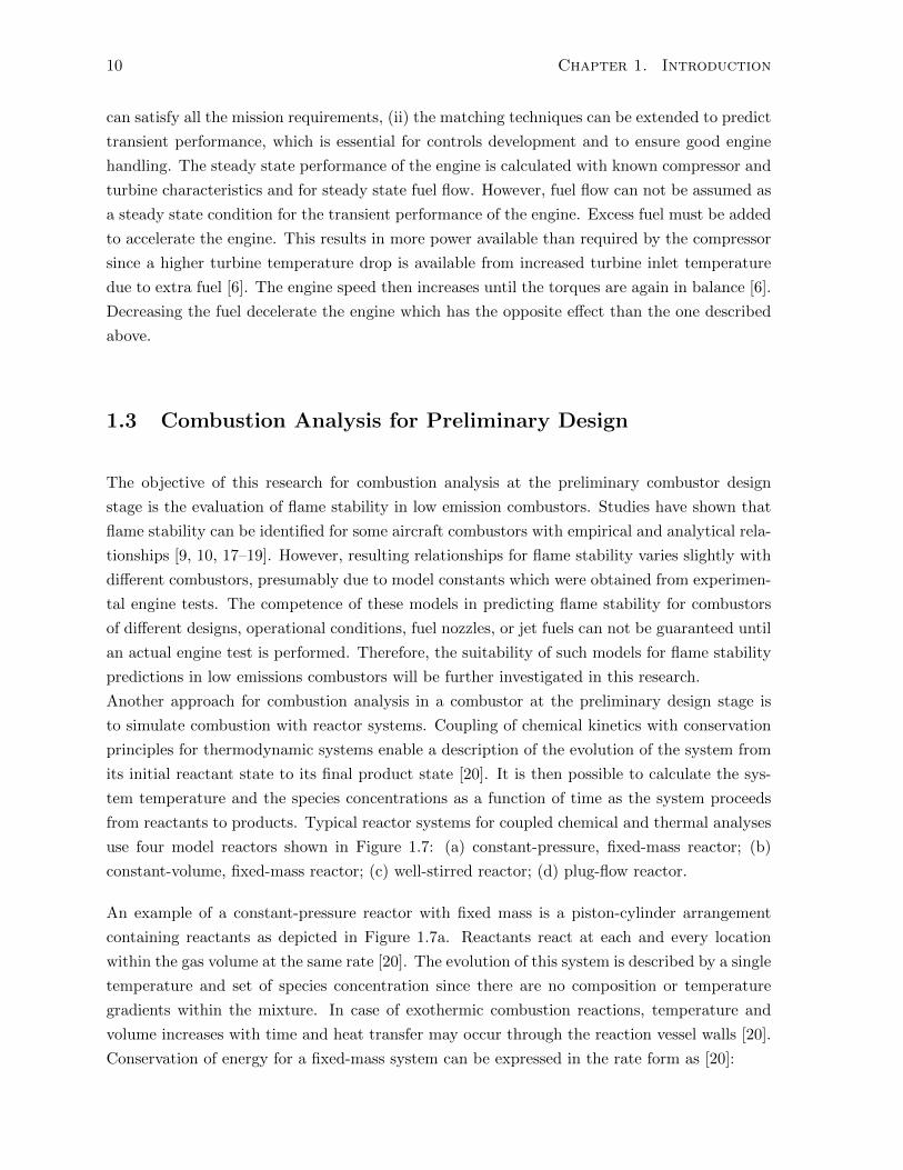
1.3 Combustion Analysis for Preliminary Design

The objective of this research for combustion analysis at the preliminary combustor design

stage is the evaluation of flame stability in low emission combustors. Studies have shown that

flame stability can be identified for some aircraft combustors with empirical and analytical rela-

tionships [9, 10, 17–19]. However, resulting relationships for flame stability varies slightly with

different combustors, presumably due to model constants which were obtained from experimen-

tal engine tests. The competence of these models in predicting flame stability for combustors

of different designs, operational conditions, fuel nozzles, or jet fuels can not be guaranteed until

an actual engine test is performed. Therefore, the suitability of such models for flame stability

predictions in low emissions combustors will be further investigated in this research.

Another approach for combustion analysis in a combustor at the preliminary design stage is

to simulate combustion with reactor systems. Coupling of chemical kinetics with conservation

principles for thermodynamic systems enable a description of the evolution of the system from

its initial reactant state to its final product state [20]. It is then possible to calculate the sys-

tem temperature and the species concentrations as a function of time as the system proceeds

from reactants to products. Typical reactor systems for coupled chemical and thermal analyses

use four model reactors shown in Figure 1.7: (a) constant-pressure, fixed-mass reactor; (b)

constant-volume, fixed-mass reactor; (c) well-stirred reactor; (d) plug-flow reactor.

An example of a constant-pressure reactor with fixed mass is a piston-cylinder arrangement

containing reactants as depicted in Figure 1.7a. Reactants react at each and every location

within the gas volume at the same rate [20]. The evolution of this system is described by a single

temperature and set of species concentration since there are no composition or temperature

gradients within the mixture. In case of exothermic combustion reactions, temperature and

volume increases with time and heat transfer may occur through the reaction vessel walls [20].

Conservation of energy for a fixed-mass system can be expressed in the rate form as [20]:

1.3. Combustion Analysis for Preliminary Design 11

Figure 1.7: Simple chemically reacting systems [20]: (a) constant–pressure, fixed mass; (b)constant–volume, fixed mass; (c) well–stirred reactor; (d) plug-flow reactor.

Q− W = mdu

dt, (1.3)

where Q is heat transfer rate, W is power rate, m is mass, u is internal energy, and t is time.

The Equation 1.3 with rearrangements for enthalpy and ideal-gas behaviour becomes [20]:

dT

dt=

(Q/V

)−∑i

(hiωi

)∑i

([Xi]cp,i), (1.4)

where T is temperature, V is volume, h is enthalpy, ω is species production rate, [Xi] is species

molar concentration, cp is constant-pressure specific heat, and variables for individual species

are denoted with the subscript i. The rate of change of the species molar concentrations is

expressed as [20]:

d[Xi]

dt= ωi − [Xi]

∑ωi∑

j[Xj ]

+1

T

dT

dt

, (1.5)


where subscript j is number of reaction. Enthalpies are evaluated with the following calorific

equation of state [20]:

hi = h0f,i +

∫ T

Tref

cp,idT , (1.6)

where h0f,i is enthalpy of formation and Tref is temperature at the reference state. The volume

is obtained from mass conservation and species production rate [20]:

V =m∑

i([Xi]MW i)

, (1.7)

where MV is molecular weight. This system of first-order Ordinary Differential Equations

(ODEs), Equation 1.4 and 1.5, describes along with equations for enthalpies, Equation 1.6, and

volume, Equation 1.7, the constant-pressure reactor.

The constant-volume reactor with fixed mass mainly differs from the constant-pressure reactor

in the absence of work (W = 0), Figure 1.7b. Then, the equation for conservation of energy,

Equation 1.3, can be evaluated as [20]:

dT

dt=

(Q/V

)−∑i

(uiωi)∑i

([Xi]cv,i), (1.8)

where cv is constant-volume specific heat. The above equation can be further expressed with

ideal gases, ui = hi − RT and cv,i = cp,i − R where R is the universal gas constant, using

enthalpies and constant-pressure specific heats [20]:

dT

dt=

(Q/V

)+RT

∑iωi −

∑i

(hiωi

)∑i

[[Xi](cp,i −R)]. (1.9)

The pressure is obtained from differentiation of ideal-gas law, with further rearrangements as

[20]:

P =∑i

[Xi]RT. (1.10)

The system of first-order ODEs, Equation 1.5 and 1.9, describes along with equations for

enthalpies, Equation 1.6, and pressure, Equation 1.10, the constant-pressure reactor.

The perfect mixing of species is provided in the well-stirred, or perfectly stirred, reactor inside

1.3. Combustion Analysis for Preliminary Design 13

its control volume [20], Figure 1.7c. This reactor differs from constant-pressure and constant-

volume reactors mainly in time dependence of such systems. The well-stirred reactor is assumed

to be operating at steady state flow conditions, so there is no time dependence in comparison

to the previous two reactor systems. Mass conservation for an arbitrary species i within an

integral control volume can be written as [20]:

dmi,cv

dt︸︷︷︸rate at which mass of i

accumulates within

control volume

= m′′′i V︸︷︷︸

rate at which mass of i

is generated within

control volume

+ mi,in︸︷︷︸mass flow of i into

control volume

− mi,out︸︷︷︸mass flow of i out of

control volume

, (1.11)

where m is mass flow rate and m′′′

is volumetric mass production rate. Variables for inlet con-

ditions are denoted with the subscript in, outlet conditions with the subscript out, and control

volume with the subscript cv. For the well-stirred reactor, assuming steady-state operation,

the Equation 1.11 becomes:

ωiMW iV + m(Yi,in − Yi,out) = 0 for i = 1, 2, ..., N species, (1.12)

where Y is mass fraction. Energy equation applied to the well-stirred reactor, assuming steady-

state operation without changes in kinetic and potential energies, is [20]:

Q = m(hout − hin). (1.13)

This Equation 1.13 can be rewritten in terms of the individual species as [20]:

Q = m

(N∑i=1

Yi,outhi(T )−N∑i=1

Yi,inhi(Tin)

). (1.14)

The solution for well-stirred reactor is found with the above equations, Equation 1.12 and 1.14,

describing the reactor as a set of coupled nonlinear algebraic equations.

And finally the plug-flow reactor represents an ideal reactor with steady state flow and no

mixing in the axial direction (molecular and/or turbulent mass diffusion is negligible in the

flow direction), Figure 1.7d. The flow is one dimensional which means that properties are

uniform in the direction perpendicular to the flow. An ideal frictionless flow and ideal gas

behaviour are assumed for the plug-flow reactor. The conservation relationships can be derived

in the following form [20]:


d (ρvxA)

dx= 0 (mass conservation), (1.15)

dP

dx+ ρvx

dvxdx

= 0 (x-momentum conservation), (1.16)

d(h+ vx

2/2)

dx+Q

′′Pm

= 0 (energy conservation), (1.17)

dYidx

+ωiMW i

ρvx= 0 (species conservation), (1.18)

where ρ is density, vx is axial velocity, A is area, x is axial distance, P is pressure, Q′′

is heat

flux, and P is local perimeter of the reactor. The solution for plug flow reactor is found with

the system of ODEs, integrated from an appropriate set of initial condition, that is obtained

from the above equations.

The mathematical descriptions are similar for the constant-pressure, constant-volume, and plug

flow reactors which all result in a coupled set of ODEs. A system of first-order ODEs is sufficient

to yield the solution describing temperature and species evolution for constant-pressure and

constant-volume reactors. A stiff equation solver is recommended to carry out the integration

in those systems [20]. Variables for the constant-pressure and constant-volume reactors are

expressed as functions of time while for the plug flow reactor variables are functions of a spatial

coordinate. For the well-stirred reactor, there is no time dependence in the mathematical model

since it is assumed to be operating at steady state. The equations describing the well-stirred

reactor are a set of coupled nonlinear algebraic equations rather than a system of ODEs [20].

Thus, the species production rates depend only on mass fractions (or molar concentrations)

and temperature. The generalized Newtons method can be used to solve this system of N +

1 equations [20] which comprises mass and energy conservation equations, Equation 1.12 and

Equation 1.14 respectively.

One possible scheme for the system of reactors representing a gas turbine combustor is depicted

in Figure 1.8. Well-stirred reactors are combined together with a plug flow reactor at the end

representing the combustor dilution zone where the mixture is supposed to be already perfectly

mixed [21]. Another possible solution with reactor network for gas turbine combustor operating

at low power was presented by Zeppieri & Colket [22]. The network is comprised of 22 perfectly

stirred reactors and its layout is shown in Figure 1.9. Simulation is focused on a characteristic

environment that a gas streak or eddy undergo in transit through the combustor rather than

on the entire combustor flow field. The reactor network model simulates the quenching process

for a partially–reacted fuel–air streak within/exiting a gas turbine combustor front–end. There

1.4. Goal of Thesis 15

Figure 1.8: Reactor network for gas turbine can [21].

Figure 1.9: Reactor network simulating the quenching process for gas turbine [22].

is no perfect layout of reactors that would perform well for various combustion problems and

types of combustors. An arrangement of reactors depends on a given problem, combustor, and

expertise of designer to achieve desired output from the reactor network.

As the result, reactor network models are useful as a first step in analyzing real devices. Reactor

networks can be further used for modelling more complex flows such as combustion in gas

turbine combustors as seen above. Simulations of reactor systems in combustors can produce

tools for emission predictions [23, 24].

1.4 Goal of Thesis

This thesis considers an analysis of combustion processes for predictions on flame stability in

low emissions aircraft combustors. The analyses include zero, one, or two dimensional semi-

empirical analytical studies of flame stability (flameout and ignition phenomena) and fully three

dimensional numerical simulations for extinction of turbulent flames in aircraft combustors.


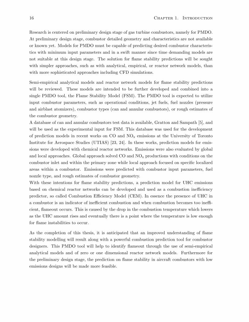
Research is centered on preliminary design stage of gas turbine combustors, namely for PMDO.

At preliminary design stage, combustor detailed geometry and characteristics are not available

or known yet. Models for PMDO must be capable of predicting desired combustor characteris-

tics with minimum input parameters and in a swift manner since time demanding models are

not suitable at this design stage. The solution for flame stability predictions will be sought

with simpler approaches, such as with analytical, empirical, or reactor network models, than

with more sophisticated approaches including CFD simulations.

Semi-empirical analytical models and reactor network models for flame stability predictions

will be reviewed. These models are intended to be further developed and combined into a

single PMDO tool, the Flame Stability Model (FSM). The PMDO tool is expected to utilize

input combustor parameters, such as operational conditions, jet fuels, fuel nozzles (pressure

and airblast atomizers), combustor types (can and annular combustors), or rough estimates of

the combustor geometry.

A database of can and annular combustors test data is available, Gratton and Sampath [5], and

will be used as the experimental input for FSM. This database was used for the development

of prediction models in recent works on CO and NOx emissions at the University of Toronto

Institute for Aerospace Studies (UTIAS) [23, 24]. In these works, prediction models for emis-

sions were developed with chemical reactor networks. Emissions were also evaluated by global

and local approaches. Global approach solved CO and NOx productions with conditions on the

combustor inlet and within the primary zone while local approach focused on specific localized

areas within a combustor. Emissions were predicted with combustor input parameters, fuel

nozzle type, and rough estimates of combustor geometry.

With these intentions for flame stability predictions, a prediction model for UHC emissions

based on chemical reactor networks can be developed and used as a combustion inefficiency

predictor, so called Combustion Efficiency Model (CEM). In essence the presence of UHC in

a combustor is an indicator of inefficient combustion and when combustion becomes too ineffi-

cient, flameout occurs. This is caused by the drop in the combustion temperature which lowers

as the UHC amount rises and eventually there is a point where the temperature is low enough

for flame instabilities to occur.

As the completion of this thesis, it is anticipated that an improved understanding of flame

stability modelling will result along with a powerful combustion prediction tool for combustor

designers. This PMDO tool will help to identify flameout through the use of semi-empirical

analytical models and of zero or one dimensional reactor network models. Furthermore for

the preliminary design stage, the prediction on flame stability in aircraft combustors with low

emissions designs will be made more feasible.

Chapter 2

Flame Stability

Flame stability is an important issue in aircraft combustors with premixed and non-premixed

combustion systems. Operational boundaries of the combustor are set by conditions beyond

which no stabilization points exist and the flame cannot be stabilized [25], called blowout

(flame is lifted and then blown to extinction). Characteristics of the leading edge of such

lifted non-premixed flames involves concepts of both premixed and non-premixed flames. Also,

non-premixed flame liftoff involves extinction process and is associated with dissipation rates

exceeding the extinction value [25]. Some premixing is happening upstream of the flame once

the flame lifts off resulting in the propagation of the flame leading edge into the premixed

reactants at the local flame speed. Therefore, the distinction between extinction and blowout

is significant for non-premixed flames. For premixed systems, flow velocities in typical aircraft

combustors exceeds the flame speed. The blowout in premixed systems is not only a concept

involving kinematic balance between flame propagation and flow velocity, but it also includes

stretch induced flame extinction. In addition, recirculating hot gases in high velocity flows add

dynamics to blowout and blowoff problems. Dynamics of near blowoff flames shown that spatio-

temporally localized extinction occurs sporadically (manifested as “holes” in the flame sheet)

but these extinction events are distinct from blowoff since flame can still persist indefinitely

under certain conditions [26]. This makes blowoff a “process” and not a discontinuous event

[25–28].

This chapter aims to describe blowout mechanisms and related processes leading to extinction

of non-premixed flames. These processes include flame interactions with strain field, such as

flame stretch, flame wrinkling, and quenching of flames by vortices or flame holes, resulting in

an extinction of non-premixed flames. Furthermore, idealized flame structures, such as edge or

triple flame structures, can be useful for description of flame extinction. Edge flame models

were recently used to characterize non-uniform flames [29]. This study closely defines flames

in highly turbulent flows, where flame extinction may be caused by holes in the flame sheet

which may open or close (“heal”). Fundamentals of above mentioned processes are given in the

17

18 Chapter 2. Flame Stability

following sections. Also, blowout or blowoff in premixed flames is reported since some flame

extinction concepts of premixed flames are related to non-premixed flames.

For the purpose of this thesis, such overview of flame stability fundamentals is critical for

the understanding of flame instabilities in gas turbine combustors, although this information

may not be directly used in the current development of prediction tools for PMDO. However,

some understandings for the development of flame stability models may arise from the follow-

ing flame stability studies in sections on “Blowout Mechanisms of Non-Premixed Flames” and

“Flow Characteristics Near Lean Blowout Limits in Model Combustors”. For instance, flame

instabilities occur in the primary zone of the combustor. Therefore, some flame stability mod-

els are focusing on this combustor zone, particularly combustion characteristic times models

are concentrating on the flame shear layer [19]. Reactor network models for flame stability

predictions should perhaps target this area as well.

2.1 Flame Extinction

This section describes flame processes and flame-flow interactions in premixed and non-premixed

flames which influence flame stability and eventually lead to flame extinction. Non-premixed

flames occur at the interface between fuel and oxidizer and do not propagate compared to

premixed flames. The burning rate of non-premixed flames in fast chemistry limit is independent

of kinetic rates and is controlled entirely by diffusive rates associated with the fuel-air mixing,

i.e. the rates at which fuel/oxidizer diffuse into the flame, while the burning rate in premixed

flames is controlled both by kinetic and diffusive rates [25]. Therefore, the burning rate of

non-premixed flame is generally only a function of the spatial gradients of fuel and oxidizer,

their diffusivities, and the stoichiometric fuel/oxidizer ratio.

Nonetheless, finite rate kinetic effect in non-premixed flames do influence burning rates and some

reactants do diffuse through the flame without burning [25]. However, this effect contributes

to the infinite fast chemistry limit as a perturbation until the spatial gradients become large

enough that the flame extinguishes.

2.1.1 Flame Stretch

Flames are sensitive to stretch, so called flame stretch, on their surface. Flame stretch is the

increase or decrease in length of material fluid elements of the flame [25], and it alters the flame

structure which may lead to flame extinction. Flame extinction is induced by high levels of

flame stretch associated with vortex-flame interactions and with separation of shear layers.

Flame sheet is stretched by the tangential velocity components, hydrodynamic stretch κa, as

well as by the effects of motion of a curved flame surface, κb, as shown in Figure 2.1. Flame

stretch rate thus yields [25]:

2.1. Flame Extinction 19

Figure 2.1: 2D flames showing positive stretching of a flame surface by [25]: (a) tangential velocitygradients along the flame, (b) motion of a curved flame (flame normal is pointing into the products).

κ =∂u-1

∂-1+∂u-2

∂-2+ ( ~vF · ~n) (∇ · ~n) = ∇- · u-︸︷︷︸

κa

+ ( ~vF · ~n) (∇ · ~n)︸︷︷︸κb

, (2.1)

where:

∇- · u- = −~n · ∇ × (~u× ~n), (2.2)

where - denotes tangential component, u- is a tangential velocity component, ~vF is velocity of

flame surface, ~n is unit normal vector to the flame, and ~u is fluid velocity vector. A distinction

exist between stretch of the material line, flame stretch κ, and stretch of a material fluid

volume, flow strain S. General hydrodynamic flow strain or deformation is given by S=

=

12

[∇~u+ (∇~u)T

].

Equation 2.1 can be rewritten to represent the role of flow nonuniformity and flame curvature

[25]:

κ = −~n~n : ∇~u+∇ · ~u︸︷︷︸κS

− su (∇ · ~n)︸︷︷︸κCurv

, (2.3)

where su is the burning velocity at flame sheet on unburned side, κCurv describes flame curvature

in a uniform approach flow leading to flame stretch, and κS incorporates the hydrodynamic

flame stretch, κa, and part of the curved flame motion term, κb. The κS expression in Equation

2.3 can be rewritten in tensor form as −ninj ∂ui∂xj+ ∂ui

∂xi.

Burning velocities for small stretch values are:

su = su∣∣∣κ=0

+∂su

∂κ

∣∣∣∣κ=0

κ = su,0 − δuMκ, (2.4)

sb = sb,0 − δbMκ, (2.5)


where superscripts u and b denote values of quantity at flame sheet on unburned or burned

side respectively, and δM defines the Markstein length. A normalized flame stretch sensitivity,

Markstein number Ma, and a normalized stretch rate, Karlovitz number Ka, can be defined

as [25]:

Ma =δuMδ0F

, (2.6)

Ka =δ0Fκ

su,0, (2.7)

where δF is the flame thickness.

The flame sensitivity to different stretch processes (κa, κb, κS , and κCurv) is identical at low

stretch rates (generally referred as the weak stretch, Ka << 1). However, at high stretch

rates the flame sensitivity to different stretch processes is not identical, e.g. the burning rates

sensitivities are different for κS and κCurv [30]. Because of gas expansion through flame at

high stretch rates, the general definition of displacement speed, sd, as the speed of the flow

with respect to the flame changes to the displacement speed with respect to the unburned and

burned flow, sud and sbd. Unfortunately, the definition of displacement speed for highly stretched

flames becomes ambiguous since the mass flux significantly varies through the flame and also

the flow velocity gradients occur over the same length scales as the flame thickness [25].

Most importantly for blowout, a maximum stretch rate that a flame can withstand before

extinguishing, κext, increases with pressure as a result of the flame thickness effect and is also

dependent on fuel/air ratio.

2.1.2 Edge Flame Structures

One-dimensional (1D) flame structures, such as plane deflagration or 1D diffusion flame, are

characterized by fundamental flame physics and two-dimensional (2D) flame structures can be

also regarded in a similar way, such as edge flames. Edge flames are idealized 2D flame struc-

tures describing flames with edges. Examples of flames with edges are illustrated in Figure 2.2

[31]. Figure 2.2a shows diffusion flame consuming most of the fuel flux (non-uniform) from the

bed, but there is a dead space between the flame and the bed introduced by neglected reaction

at the temperature of the bed surface, giving the flame an edge. Figure 2.2b shows a candle

flame in microgravity conditions. The flame is hemispherical in shape and has circular edge.

which remains stationary or oscillates up and down prior to extinction. Figure 2.2c shows a

diffusion flame affected by turbulence and its quenching, producing flame holes if scalar dissi-

pation rates are large enough. Each of these holes has an edge and also an edge for surrounding

1D flame. Another similar situation to Figure 2.2a is depicted in Figure 2.2d, illustrating a

2.1. Flame Extinction 21

(a) (b) (c) (d)

Figure 2.2: Edged flames [31]: (a) flame spreading over a fuel-bed, (b) candle flame burning undermicrogravity conditions, (c) wrinkled torn flame in turbulent flow, (d) diffusion flame sitting on a plate

through which fuel is injected.

Figure 2.3: Edge flame configurations [25]: (a) fuel/oxidizer interface with quasi-one-dimensionalnon-premixed flame downstream, (b) premixed flame in shear layer with quasi-one-dimensional

premixed flame downstream, (c) ignition front, (d) flame holes induced by local extinction.

plate through which fuel is injected and air passes over this plate. 1D diffusion flame with an

edge is located in the formed reactive boundary layer.

Edged flames are defined by a concept describing propagation of their structures at well de-

fined velocities having unchanged shape [31]. A structure of unstretched and stretched flames

generally exhibits “edges” as most real flames do [25], and thus introducing additional physics

compared to flames with continuous fronts. High gradients in flame-normal and tangential

directions are present in edged flames. These edges are important for understanding the non-

premixed flame stabilization at fuel/oxidizer interfaces, propagation of an ignition front, or the

flame holes induced by local extinction [32], see Figure 2.3. In turbulent combustion, the be-

havior of the flame, flame edges, or flame holes is affected by the curvature, hence flame edges

are curved [31].

The main behaviours of the flame edge are distinguished by its velocities as follows: stationary

edge, advancing edge into fresh gases as an ignition wave, and retreating edge as a “failure

wave” [25, 31]. The flame edge propagates in premixed flames and even in non-premixed flames

in which the flame does not propagate as mentioned earlier. In non-premixed flow, advancing

edge flames are characterized by positive edge flame velocity, i.e. an ignition front (vF > 0),

and retreating edge flames are characterized by negative edge flame velocity, i.e. an extinction

front (vF < 0).

Moreover for an advancing flame, the three branched structure, so called “tribrachial flame” or


(a) (b)

Figure 2.4: Flame structures: (a) tribrachial flame supported by weak mixture gradients in the supply[31], (b) edge flame hole opening (flow with spatially varying stretch rate) [25].

“triple flame”, is present due to significant premixing at an ignition front and to the presence of

trailing diffusion flame [25, 31]. A non-premixed flame is connected to rich and lean premixed

flame at triple point [33]. Figure 2.4a shows deflagration in the mixture moving in the z-direction

in which the fuel and oxidizer vary linearly in the x-direction [31]. Mixture proportions are

as follows: stoichiometric on the z axis, fuel-lean in x < 0, and fuel rich in x > 0. With this

composition, the burnt gas contains hot unburned oxidizer in x < 0 and hot unburned fuel in

x > 0. As these excess reactants diffuse toward each other a diffusion flame that trails the two

branches of the premixed flame is generated.

In unstretched flames, heat losses are a significant factor and alter flame properties [34]. In

highly stretched flames near extinction, loss process is dominated by diffusive losses associated

with strong gradients and heat losses are of secondary importance and therefore flame is usually

treated as adiabatic. However, heat losses may be an important factor in highly stretched

flames if the flame edge is near boundaries. Effects of heat losses on a flame are illustrated in

Figure 2.5a, showing that high stretch rates or high heat losses can lead to negative edge flame

propagation (retreating flame edge), and in Figure 2.5b, relating heat loss with with Damkohler

number.

Flow with spatial gradients in stretch rate at the flame edge can lead to formation of flame

holes, see Figure 2.4b. Flame extinguishes at points at which the extinction stretch rate of a

continuous flame sheet, κext, is surpassed by local stretch rate, κ. Steady state of the flame edge

is denoted by κedge. Initially, premixed flame front with no holes is exposed to a spatial stretch

rate gradient. A hole can occur when a flame is in a region of high stretch rates. This leads to

flamelet extinction at adjoining points once a hole initiated. However under local conditions,

these points would not have extinguished [25]. Nonetheless, flame holes in premixed flames

introduce mass and energy transport between reactants and products. This is favourable to a

flame since it leads to dilution, preheating, and radical introduction into the reactants [25].

2.2. Flame Stabilization 23

(a) (b)

Figure 2.5: Edge flame dependencies [25]: (a) calculated edge speed dependence on Damkohler numberof premixed flames [35], (b) effects of the Damkohler number and heat loss on flame regimes of

non-premixed flames [29].

Quenching of a non-premixed flame by vortex was simulated by Favier and Vervisch [36] and the

mechanism was described as follows: a flame hole is initially formed, the recession of the flame

edge follows (negative edge velocity), the flame edge advances to close the hole once the vortex

has passed (positive edge velocity). A relationship between κedge under steady conditions and

κext was developed into [37, 38]:

κedgeκext

=e2

(1− T0/Tad)

RuTadEa

, (2.8)

where internal energy is e≈2.718, T0 is the ambient temperature, Tad is the flame front tem-

perature for an adiabatic uniform nonpremixed flame with complete reaction, Ru is universal

gas constant, and Ea is the activation energy. Measurements indicate ranges of stretch rates

fraction of 0.5 < κedge/κext < 1.0 [38–41].

2.2 Flame Stabilization

Multiple flame stabilization points can exist as flames exhibit different shapes and lengths.

For non-premixed flames, a flame that finds stabilization points can spread downstream with

location where fuel and oxidizer are in stoichiometric proportions [25]. For premixed flames,

this location is controlled by the kinematic balance between flame and flow speed.

2.2.1 Stabilization and Blowoff Mechanisms of Premixed Flames

Figure 2.6 shows four premixed flame configuration in an annular, swirling model combustor.

The configuration (d) is typically observed in low velocity flows and other three shapes of the

flame are formed if the flame cannot stabilize in both inner and outer shear layer [25]. This


Figure 2.6: Basic premixed flame configurations for an annular, swirling model combustor [25].

(a) (b)

Figure 2.7: Blowoff concepts in premixed flames [25]: (a) transverse dependence of the laminar burningvelocity and flow velocity, (b) dependence of the critical blowoff and flashback gradients of natural

gas/air mixtures on equivalence ratio.

configuration (d) bifurcates to configuration (c) if the flame cannot anchor in the outer shear

layer. The configuration (c) may bifurcate to configuration (a) if the flame cannot anchor in

the inner shear layer. A sequence of local blowoff events may be considered as the shifts in

flame location and blowoff occurs if no stabilization locations are possible. Aforementioned

mechanisms are more related to applications in power generation than to aircraft applications.

Blowoff in premixed flames occurs when the flow velocity is everywhere greater than the up-

stream propagation velocity of the combustion wave [25]. Figure 2.7a shows the blowoff concept

with different velocity gradients: gu,a, gu,b, and gu,c. Flow velocity increase linearly from zero

at the wall with a velocity gradient gu. Laminar burning velocity, sud , is present in the core of

the flow but drops to zero within the quenching distance, δq, from the lip. A situation with

line a corresponds to flow velocity everywhere greater than sud and therefore the flame will blow

off due to this proportion in velocities and not because of the flame extinction. A situation

with line b shows a stabilization point, sud = ux, from which the flame propagates into the core.

In the last case c, the flame will propagate upstream since sud > ux. Figure 2.7b depicts the

relationship between blowoff and flasback gradients on the equivalence ratio [25]. A stationary,

stable flame is possible in the region between flashback and blowoff values; this region is called

the operability window of the burner.

Flame holes are generally initiated in high stretch region, but interestingly not near the bluff

body where the stretched rate is highest. This is due to the fact that stabilization point consist

2.2. Flame Stabilization 25

of reactants diluted with hot products [25]. However, the flame cannot withstand high stretched

levels further downstream. As the result, flames near blowoff levels often do not extinguish near

the stabilization point but instead extinguish downstream of it.

2.2.2 Blowout Mechanisms of Non-Premixed Flames

Extinction of jet diffusion flames is usually described by their liftoff and blowout characteristics

[42]. Turbulent flames exhibit both local and global extinction due to excessive straining or other

limitations. Several theories describe the stabilization of lifted turbulent non-premixed flames,

e.g. mixing of the flame base upstream [43], quenching of laminar flamelets [44], propagation of

triple flamelets and/or edge flames in partially premixed reactants [45–47], or conditions were

identified for flames that are blown out as soon as they are lifted from the burner [45, 48].

The experimental study by Chao et al. [49] showed that blowout of a tubulent jet diffusion

flame happens rapidly and unpredictably as a transient process with a series of consecutive

events. Flamefront instabilities affect the blowout process and flame base pulsation and flame

flickering usually occurs before the flame blows out [50, 51]. Nonetheless, the detailed blowout

mechanism is still not clear.

Wu et al. [52] investigated experimentally turbulent jet diffusion flames and proposed a blowout

mechanism based on triple flame and stoichiometric contour. They concluded that the blowout

process depends on initial velocity or Reynolds number and gas properties at the jet exit without

knowing the local flame-flow conditions of the liftoff flame near blowout [52]. The proposed

mechanism is based on flame-base behaviour of the blowout process and is sorted into four

characteristic regions as shown in Figure 2.8: the pulsating, onset of receding, receding, and

extinction regions. Triple flame structures are found in the flame base, pulsating, and onset

of receding regions. Flame base locations in each regions correspond to the stoichiometric and

lean limit contours of the premixed model. Pulsation region is characterized by stabilization

and pulsation of the stabilization point of the triple flame along the stoichiometric contour.

Recession and extinction of the flame is caused by diminution of the stoichiometric branch of

the triple flame and by the fuel-lean condition.

In detail, initially the flame base region is described with the jet velocity, U0, being between the

liftoff velocity, Ul, and the blowout velocity, Ub, and with the lifted flame stabilized in the range

upstream of the maximum “waistline” point of the stoichiometric contour, Figure 2.8b. The

flame steps into the pulsating region and become unstable if the flame base of the lifted flame is

pushed beyond the maximum waistline point while the jet exit velocity is equal to the blowout

velocity, Figure 2.8c. The triple flame is found here in the flame base and its stoichiometric

branch acts as the stabilization point. This flame base has boundaries consisting of lean and

rich limits. The flame becomes lean when the stabilization point and the stoichiometric branch

of the triple flame vanish as the flame base is pushed downstream and the flame is pushed


Figure 2.8: Schematic of the proposed blowout process mechanism [52].

beyond the tip of the stoichiometric contour, Figure 2.8d. The flame recedes downstream and

eventually extinguishes, Figure 2.8e.

Han and Mungal [53] carried out an experiment on the transition from flame liftoff to flame

blowout of a non-premixed turbulent jet flame. Two simple methods to blow out a stable

lifted flame exist: either to increase the jet velocity or to increase the coflow velocity. They

compared a stable lifted flame with a lifted flame near blowout. The near-blowout condition

was obtained with variations in the coflow speed of the lifted flame in coflow. A simple blowout

mechanism was proposed with the flame stabilization concept of the leading edge flame. The

blowout mechanism was defined as follows: movement of the flame base to a higher velocity

region corresponds to a movement of the flame surface through a change of the stoichiometric

velocity, the flame blows out if the higher velocity is not sustainable by the flame base.

Iyogun and Birouk [54] performed an experiment on the stability of a turbulent, non-premixed

methane flame. The burner was surrounded by an annulus of co-airflow with varying swirl

strength. They tested two different central fuel nozzles with similar exit cross-sectional areas

but with different internal orifice geometry, a Rectangular Nozzle (RN), and Contracted Circular

Nozzle (CCN). It is believed that swirl enhance flame stability by generating a recirculating

vortex and shortens the the flame length. However, the flame length increases as the swirl

2.3. Flow Characteristics Near Lean Blowout Limits in Model Combustors 27

(a) (b)

Figure 2.9: Simultaneous PIV and OH-PLIF measurements showing the stabilized flame close to LBO[55]: (a) vertical section, (b) horizontal section.

lenght increases until a critical swirl number is reached, after which the flame length starts to

decrease with the increasing swirl. The swirl also introduces large scales important for mixing,

but small scales are important for chemical reactions. As the result it was found that blowout

for the RN is higher than the one for the CNN, and also that the liftoff velocity, liftoff height,

and flame length are lower for RN compare to CNN.

2.3 Flow Characteristics Near Lean Blowout Limits in Model

Combustors

The experimental research on flame stability, particularly on flameout characteristics, to date

has been mostly conducted using model combustors representing actual aircraft combustors.

Experimental studies of model combustors offer insights into flame stability phenomena possibly

applicable in aircraft combustors. Model combustors are characterized by confined swirl flames.

The flow fields of the model combustors all generally featured fresh gas stream forming a cone-

shaped flow when entering the combustor from a burner nozzle, inner recirculation zone (IRZ),

and an outer recirculation zone (ORZ). A closer study of near LBO limits has been enabled with

modern techniques of experimental flow visualization and measurements. A brief summary of

a few relevant studies now follows.

A model combustor was studied by Stohr et al. [55] using chemiluminescence imaging, simulta-

neous stereo Particle Image Velocimetry (stereo-PIV), and Planar Laser Induced Fluorescence

of OH radicals (OH-PLIF) measurements. The study showed that close to the LBO limit there

are two main regions where reaction takes place, the helical flame zone and the flame root, as


(a) (b)

Figure 2.10: Swirl number of CH4 fuel in swirling non-premixed combustor [58]: (a) flame stabilityregions with various swirl numbers, (b) flame images near the lean blowout limit (Ufuel = 6m/s and

Uair = 8m/s) and the rich blowout limit (Ufuel = 84m/s and Uair = 8m/s).

shown in Figure 2.9. The helical flame zone occurs along a precessing vortex core (PVC) at the

inner shear layer (ISL) in the flame [56, 57]. This zone is favorable to flame since it provides

low strain rates and accelerated mixing of burned and fresh gas. The flame root is located right

above the nozzle around the lower stagnation point and is formed by an opposing flow of fresh

gas from the nozzle and burned gas from the IRZ.

Hwang et al. [58] studied flame blowout limits in a swirling non-premixed combustor for land-

fill gas mixed fuels (landfill gas-liquified propane gas). The effects of a swirl conditions on

flame blowout were investigated. Under strong swirl conditions, the heating value of the fuel

determined the blowout velocity (with a linear dependency). Under weak swirl conditions,

the blowout velocity decreases in proportion to the CO2 ratio of mixed fuels (CO2 − CO2)and

increases in proportion to the stoichiometric air/fuel ratio of the fuel. Their results for flame

stability regions, Figure 2.10b, can be useful for understanding of flameout phenomena.

Durbin and Ballal [59] studied LBO in a unique Step Swirl Combustor (SSC) simulating fuel-

air mixing patterns. These patterns were produced by an airblast atomizer located in the

combustor dome of an annular gas turbine combustor. As the result, an increased outer swirl

intensity improves LBO. For the same SSC, Durbin et al. [60] found the flame lifts from the

fuel tube and is stabilized by the inner recirculation zone when inner swirl velocity is higher.

Furthermore, LBO values are found to be higher for a lifted flame than for an attached flame.

Counterswirl conditions produced attached flames for moderate inner velocity, and for higher

inner velocity both co- and counterswirl produce lifted flames with similar LBO values.

Chapter 3

Flame Stability Modelling

In what follows, previous theoretical, experimental, and numerical studies of flame stability,

particularly for flameout in aircraft combustors, are reviewed. Flame stability evaluations

throughout the complete combustor design cycle may be obtained from the presented models.

Semi-empirical analytical models can be used for the preliminary design stage. Complex numer-

ical models can be perhaps used at the detailed design stage when the exact dimensions of the

combustor are known. Then, such models can be even complementing preliminary design with

more accurate input data for semi-empirical analytical models. However, complex numerical

models, in particular models for CFD simulations, would first need to be capable of predicting

blowout with some accuracy.

3.1 Semi-Empirical Analytical Models for Flame Stability

Two types of semi-empirical analytical models evaluating flame stability in aircraft combus-

tors can be generally found in the literature, models are either based on combustor loading

characteristics or on characteristic times of combustion inside the combustor. The combustor

flame stability characteristics are generally represented by plotting fuel/air ratio (equivalence

ratio) of the combustor primary zone at blowout against some form of loading [2]. Such model

is hereafter called a Loading Parameter Model (LPM). Flameout can be also modelled by the

approach that is based on the characteristic times of combustion. Characteristic times are order

of magnitude estimates implemented as an algebraic expressions, so called Characteristic Time

Model (CTM), and then used to represent the flame stability and/or ignition properties of the

combustor. Detailed description of these two types of semi-empirical analytical models, their

modified versions, and other types of models for flameout are provided in following subsections.

29

30 Chapter 3. Flame Stability Modelling

3.1.1 Characteristic Time Models

The stabilization of turbulent premixed flames in a combustor can be interpreted by Damkohler

number as [20]:

Da =τflowτchem

=

> 1, stable

< 1, unstable, (3.1)

where τflow is the characteristic flow or mixing time (also characterized as lifetimes of large

eddies in the flow) and τchem is the characteristic chemical time [20]. The flame is stable if

Damkohler numbers are greater than unity and unstable with Damkohler numbers below unity.

This relationship can be expressed for Damkohler number at blowout [9]:

Dab =τslτhc

=

> 1, stable

< 1, unstable, (3.2)

where τsl is the shear layer residence time of fuel droplet and τhc is the ignition delay time. In

this equations the characteristic flow and chemical times were replaced by characteristic fuel

droplet times. Unfortunately, neither of these characteristic times can be estimated exactly in

a combustor [9].

Mellor [61] suggested five characteristic times for combustion and pollutant formation in two-

phase turbulent flow, Figure 3.1: the fuel droplet lifetime, τeb; the eddy dissipation times for

injected fuel τfi, and in the shear layer, τsl; the fuel ignition delay and burning time, τhc; and

the NO formation time, τno. A relationship between these times for continuous combustion in

heterogeneous systems is [18]:

τsl ≥ τhc + τeb, (3.3)

and at the blowoff limit:

(Tin/Tφ=1)τsl ∼ τhc + kτeb, (3.4)

where k is a constant and Tin is an inlet temperature (temperature ratio describes here an

acceleration due to heat released in the shear layer). This criterion for the blowoff limit,

Equation 3.4, says the shear layer (surrounding the recirculation zone which holds the flame)

provides the mixing time which must be sufficient both to ignite the mixture and to evaporate

the fuel.

3.1. Semi-Empirical Analytical Models for Flame Stability 31

Figure 3.1: CTM - Schematic for shear layer details in combustor [17].

Shear layer residence time, τsl, represent the length of time the fuel is in the initial shear layer

and for a turbine combustor is:

τsl = τsl,co = lco/Vref , (3.5)

where reference velocity, Vref , is air velocity at the maximum combustor cross-section area (an

area based on compressor discharge conditions, i.e. an area between inner and outer casing

walls) and characteristic length, lco, is a function of the primary or secondary length, lpri,sec

and combustor annulus height or diameter, lco−1 = lpri,sec

−1 + dcomb−1 [62].

Ignition delay times, τhc, estimate the time for the fuel to ignite once the fuel is evaporated.

Plee and Mellor [18] correlated τhc based on the experimental data from Ballal and Lefebvre

[63] into the equation:

τhc = 10−4 exp[E/RTφ=1]

φpz(ms), (3.6)

where Tφ=1 is the adiabatic, stoichiometric flame temperature and φpz is the equivalence ratio

in the primary zone. The pre-exponential constant, 10−4, and the activation energy, E = 21.0

kcal/gmole, are determined empirically.

The droplet evaporation time is evaluated with the d2 law of Godsave [64]:

τeb = do/β (ms), (3.7)

where do is the initial diameter corresponding to Sauter mean diameter of the fuel spray and β

is the evaporation coefficient with forced convection assumption.

Finally, the CTM was developed into the complete correlation form for the blowoff limit [18],

Figure 3.2:


Figure 3.2: Characteristic time correlation for blowoff limit [9].

τsl + 0.12τfi′ = 2.12(τhc

′ + 0.011τeb′) + 0.095, (3.8)

where the primes denote the inclusion of temperature ratio (Tφ=1/Tin) from the Equation 3.4

and heterogeneous effects are included with τfi and τeb. For practical gas turbine systems, τfi in

Equation 3.8 will be zero since high momentum quench air through discrete air-addition holes

minimize strong fuel penetration effects.

Mellor CTM

Plee and Mellor [18] obtained the following CTM for the blowoff limit in gas turbine combustors:

τsl = m(τhc′ + 0.011τeb

′) + b, (3.9)

where again τsl is the eddy dissipation time in the shear layer, τhc is the fuel ignition delay

and burning time, τeb is the fuel droplet lifetime, and constants m (slope) and b (intercept)

are determined experimentally from run data of an actual aircraft combustor. According to

Mellor [17], τsl is a function of combustor geometry and inlet conditions, τhc a function of inlet

conditions and fuel properties, and τeb a function of fuel properties and fuel injector atomization

capabilities.

Flameout is predicted by Equation 3.9 when the right hand side is greater then the left hand side

[17]. Model constants, m and b, necessary for an evaluation of flame stability were successfully

obtained from experimental tests of various combustors. Experimental results from combustors

tests were correlated for can and annular combustors with the following model constants: m =

2.12 and b = 0.095 for can combustors by Plee and Mellor [18], m = 1.33 and b = 0.25 for annular

combustors by Jarymowycz and Mellor [19] investigating the J85 engine. Then, it should be


(a) (b)

Figure 3.3: Predictions of TF41 combustor limit conditions at altitude [69] (solid line is for predictionsand dotted line is for measured data): (a) lean blowoff models, (b) ignition models.

possible to use this model without performing an actual experimental combustor test. However,

different model constants were reported from other engine tests. Lean blowoff limits for aviation

engines J85 (General Electric), T-63 (US military designation for Rolls-Royce M250, formerly

Allison 250) and AGT-1500 (Honeywell) were obtained by CTM correlations with constants

m = 1.36 and b = 0.36 by Derr and Mellor [65]. Although different fuels were used in above

researches for various combustors, these constant may still differ with identical test conditions

of similar combustors. Therefore, these differences in model constants possibly indicate that

this model cannot be overly generalized to account for main combustors configurations, for

instance to account for all annular combustors with the identical model constants. This model

utilization for flame stability predictions should be further investigated.

The ignition process is modelled by a similar procedure [17, 66–70]. Peters [69] applied the

aforementioned model for flame stability, Equation 3.9, and also an ignition model to TF41

combustor. Changes in combustor performance were predicted with the use of alternative fuels,

Figure 3.3.

3.1.2 Loading Parameter Models

A combustor loading parameter (LP) can be obtained from a reaction rate theory when regard-

ing the combustor as a well stirred reactor [71]. Thereafter, a Perfectly Stirred Reactor (PSR)

can define LP as

LP =mcomb

PnVcombF, (3.10)


where, mcomb is mass flow in combustor, Pcomb is combustion pressure, n is a constant rep-

resenting the apparent reaction order, Vcomb is a combustor volume, and F is an exponential

temperature factor to correct reactants inlet temperature.

For a single-step bimolecular reaction, the theoretical value of n is 2. The parameter n is a

function of pressure and equivalence ratio and n increases with increasing equivalence ratio and

decreases with increasing pressure. Kretschmer and Odgers [72] recommended n = 2φ for lean

mixtures and n = 2 for rich mixtures (φ > 1) at atmospheric and subatmospheric pressure. For

burning rates of adiabatic premixed hydrocarbon/air flames, n falls into the limit 0 < n ≤ 2.

The value of n can be determined experimentally for a given combustor operating over a range

of representative conditions.

Lefebvre [10] has derived relations for flame stability and ignition of aircraft combustion cham-

bers by expressing overall combustor fuel/air ratio. This ratio is the limit under flame extincts

or ignition is not possible.

For homogeneous mixtures (fuel vapour and air mixture), the relationship between fuel/air ra-

tio at blowoff and properties of the burner inlet air and the volume of the combustion zone is

[17]

qLBO ∼mA

VpzP3n exp (T3/b)

, (3.11)

where mA is the total airflow rate, Vpz is a combustor volume in the primary zone, n is a

pressure and equivalence ratio constant, and b is a temperature constant.

For heterogeneous mixtures (liquid fuel and air mixture), the fraction of fuel that is vaporized

within the primary zone, ff , is considered and the fuel/air ratio at lean blowout is [2]

qLBO(heterogeneous) = qLBO(homogeneous)/ff . (3.12)

From analysis for fuel spray evaporation rate [2] it was found that:

ff =8ρgVcλeff

fpzmADo2 , (3.13)

where ρg is density of gas, Vc is the combustor volume, λeff is the effective evaporation constant,

fpz is the fraction of air employed in the primary zone (i.e. the fraction of mA entering the

primary zone), and Do is the initial drop diameter.


Lefebvre LPM

Lefebvre [10] derived a relation for flame stability of aircraft combustion chambers in terms of

the overall combustor fuel/air ratio. This ratio is the limit under which flame extincts. The

lean blowout fuel/air ratio, qLBO, was derived for heterogeneous mixtures from lean blowout

data of aircraft combustion chambers into the form [10]

qLBO =

[A

Vpz

][mA

P31.3 exp (T3/300)

][Dr

2

λrHr

], (3.14)

where again mA is the total airflow rate, Vpz is a combustor volume in the primary zone, Dr is

the mean drop size, Hr is the lower calorific value, and λr is the effective evaporation (all values

are relative to JP4 fuel [2]). The first term on the right hand side of Equation 3.14 represents

the combustor design, the second term represents the combustor operating conditions and the

third term represents the fuel properties. Here, A is a combustor-specific constant dependent on

the combustion zone (geometry and mixing characteristics) and on the amount of air employed

in primary combustion [10]. Therefore, the value of A must be determined with an actual

operation data [17] and its values are shown in Table 3.1. According to Lefebvre, this equation

can be used to estimate the lean blowout fuel/air ratio at any operating condition once A is

determined at any convenient test condition [2].

For homogeneous mixtures, the lean blowout fuel/air ratio, qLBO, was derived from lean blowout

data of aircraft combustion chambers and found to have the form [2]:

qLBO = C

[mA

VcP31.25 exp (T3/100)

]0.16

, (3.15)

where C is a combustor-specific constant which must determined experimentally for each com-

bustor. The Equation 3.15 was obtained by substituting for mA = ρUA into the equation of

weak extinction for bluff-body flameholder operating with homogeneous mixtures [2]:

φWE ∝[

U

P 0.25To exp (To/150)Dc(1−Bg)

]0.16

, (3.16)

where U is the velocity in the plane of the flameholder, P is the pressure, To is the inlet gas

temperature, Dc is the characteristic dimension of the flameholder, and Bg is the blockage ratio.

Engine J79-17A J79-17C F101 TF41 TF39 J85 TF33 F100

A 0.023 0.032 0.042 0.031 0.064 0.025 0.037 0.013

Table 3.1: Values of A employed in Equation 3.14 for aircraft engines, [2].


(a) (b)

Figure 3.4: Comparison of J85 combustor measured and predicted values of [2]: (a) qLBO withEquation 3.14, (b) qLLO.

The ignition characteristics, such as the lean lightup fuel/air ratio qLLO, are determined simi-

larly to the aforementioned flame stability characteristics [10]. Equation 3.14 for flame stability

and an ignition equation were evaluated for the J85 combustor [2], see results in Figure 3.4.

Rizk-Mongia LPM

Rizk and Mongia [73] merged Lefebvre’s models and pattern factor (TDF - Temperature Distri-

bution Factor), with the 3D computer code resulting in the hybrid equation for the local value

of fuel/air ratio at lean blowoff:

qlbo,i =

[A

ma,iTi/Pi

][ma

P31.3 exp (T3/b)

][mev,i

mf,i

][trHr

]mB,i, (3.17)

where the subscript i refers to the ith volume element of the 3D CFD grid, tr is the ratio of

evaporation times at LBO and reference conditions, T is temeprature, mev is the fraction of

fuel evaporated, mf is the fraction of fuel evaporated and burned, and mB is the fraction of fuel

burned. This expression was used to estimate lean blowoff in each computational cell and in

the solution domain in order to predict the overall blowoff in the combustor. The CFD solution

method was applied to two power conditions (47% and full power) to determine the values of

mev, mf , mB, and T in each of the volume elements. A value for A was set by comparisons

of combustor data for blowoff at the same power conditions. The value of A was subsequently

held constant for predictions on blowoff fuel/air ratios at other power levels.

3.2. Numerical Modelling of Flame Stablity 37

3.1.3 Other Models

Another approach for flame stability modelling is based on the reaction-quench model which

was introduced by Ballal and Sturgess [74]. This model assumes that flame propagation at lean

blowout (LBO) limit will cease when the rate of mixing between small turbulent eddies of cold

reactants and hot products is greater than the local chemical reaction rate. Their quenching

criterion yields [74]

1.5(D + CµK

2/σtε)

ν (1 + SL/(εν)0.25)> 1, (3.18)

where D is the laminar diffusion coefficient, Cµ is a constant, K is the kinetic energy of turbu-

lence, σt is the turbulent Schmidt number, ε is the dissipation rate, ν is the kinematic viscosity,

and SL is the laminar flame speed. The Equation 3.18 originates from work of Lockwood and

Megahed [75] introducing criterion when flame will be quenched

D/U > η, (3.19)

where D is the diffusion coefficient, U is the flame speed, and η is the Kolmogorov microscale.

The criterion is based on two neighboring microscale vortices with an interface area A. Flame is

quenched whenever the volumetric interdiffusion of hot and cold molecules, I = AD/η, exceeds

the volumetric rate of chemical reaction, R = UA.

Isothermal flow CFD calculations were performed at each grid node to provide turbulence

parameters required by the quenching criterion of Equation 3.18 above. Conditions for the

CFD evaluation were [74]: (i) quenching is examined on a point-by-point basis to ascertain if

any part of the flow field could support the combustion, (ii) local fuel/air ratio must be within

flammability limits, and (iii) local mean velocities should be less than or equal to turbulent

velocity. This approach outlines operating conditions of a step combustor where combustion is

or is not possible and also provides the reactor extinction criteria for the subgrid-level stirred

reactor modelling [74].

3.2 Numerical Modelling of Flame Stablity

Combustion models for flameout and ignition prediction using high fidelity CFD are reviewed in

this section. A current overview for the simulation of combustion processes related to flameout

and ignition is presented. Also, a way for simulation of turbulent flames for flameout was

attempted to describe.


Unsteady combustion with complex chemical reactions and high turbulent flows present in air-

craft combustors is challenging task for numerical simulations, especially for flame stability

modelling. Chemically reacting turbulent flows are primarily simulated with the following nu-

merical approaches: Direct Numerical Simulation (DNS); Large-Eddy Simulation (LES); and

Reynolds-Averaged Navier-Stokes (RANS).

The DNS is the most accurate approach resolving all scales of flow, free of additional scales

modelling but disadvantaged by immense time demand (often refereed as the computational

cost). A time demand limits this approach for complex engineering application except of proven

DNS power in fundamental studies, such as specific combustion or turbulence studies of flame

extinction, flame-turbulence or flame-wall interactions, and so on [76–80].

The RANS method averages governing equations with averaged flow variables without resolv-

ing turbulent fluctuations which need to be entirely modelled [81]. Unfortunately, an entire

modelling offers a limited flexibility for unsteady flow [82–84].

The LES method and its computational cost lies between DNS and RANS approaches. The

LES and employs low-pass filtering procedure separating scales where the flow is directly (ex-

plicitly) resolved in the large scales motions whereas the effects of small (unresolved) scales are

modelled [85]. In spite of unemployed full LES potential due to incomplete combustion theory,

the LES solves unsteady combustion, combustion instabilities [86–88], and other various com-

bustion problems [89–95].

Complex chemical reactions stem from the increased level of fuel mixedness caused by more

developed turbulence. However, these effects are not fully addressed in the above mentioned

traditional numerical methods for a reasonable computational cost. The answer for fuel-lean

non-premixed flow lies in the combination of different numerical approaches fully incorporating

turbulence and complex chemistry.

Ganji and Ebrahimi [96] have used the Eddy Dissipation Concept model (EDC) to perform

blowout studies of hydrogen-air mixture in a micro gas-turbine chamber. The EDC model

introduces mean reaction rate by empirical expression assuming the chemical reaction takes

place in region where the dissipation of turbulent energy occurs. Equations expressed by Gran

and Magnussen [97] for reactive volume fraction of the flow ξ3, time scale τ for mass transfer

between fine structures and surroundings, and the mean reaction rate Ri form the EDC model:

ξ =

(3CD2

4CD12

)1/4 (νεk2

)1/4, τ =

(CD2

3

)1/2 (νε

)1/2, Ri =

ρξ2

τ(Y ∗i − Y ◦i ) , (3.20)

where model constants CD1 = 0.134 and CD2 = 0.5 are obtained from energy cascade model,

ν is the kinematic viscosity, k is the turbulent kinetic energy, ε is the turbulent dissipation

rate, Yi∗ is the mass fraction for species i inside fine structures, and Yi

◦ is the mass fraction for

species i in surroundings. During time τ , fine structures are assumed as PSR under constant

3.2. Numerical Modelling of Flame Stablity 39

pressure and adiabatic conditions and Arrhenius relations control the reaction progress. The

transport equations of the k-ε Reynolds Averaged Navier Stokes (RANS) viscous model are

solved in order to obtain value ε for EDC model. The chemical kinetic mechanism of hydrogen

oxidation was employed in this simulation. However, the high amount of reaction rate causes

the simulation predicts combustion inside the cooling jacket whereas the combustion is limited

to area inside the combustion chamber according to experiment results. This was corrected

with a restricted reaction rate which was found to predict the combustion area to be inside the

chamber. A restricted reaction rate was calculated with EDC model (considering molecular

scale mixing time and a PSR assumption), which predicts blowout at different mass flow rates

and equivalence ratios.

Predicted mass flow rates for stable combustion by simulation of EDC combustion model with

disabled turbulence productions and turbulent viscosity source terms in RNG k-ε transport

equations were in agreement with experimental results [96]. This implies that such model can

be considered as an available engineering approach for blowout predictions [96].

Wetzel et al. [98] investigated LBO combined model of a model gas turbine combustion cham-

ber and found that convective and radiative heat loss processes should be included for LBO

predictions. They developed a LBO model consisted of the following approaches: a convective-

diffusive problem was solved by a finite volume approach with RANS method using the stan-

dard k-ε turbulence model, the interaction of turbulence and chemical reaction was solved by

Joint-probability-density model with an assumed shape of the Probability-Density-Function

(presumed shape JPDF model). It was concluded that the LBO is predicted at much lower

thermal loads when heat loss processes are included.

Neophytou et al. [99] built a model for predicting ignition probability of turbulent recirculating

non-premixed gas flames. The CFD model uses information from the flow field patterns before

ignition and calculates possible flame trajectories of emanating flame from a spark. Equations

for turbulent mixing are based on the standard Lagrangian description [100] and capture the

flame particle motion. Particles are tracked in the CFD solution of the cold flow that is gen-

erated with RANS method. Trajectories calculations uses data of the laminar burning velocity

in sprays and include flame extinction (capturing of the flame quenching), mixture fraction

calculation (capturing of the flame non-premixed nature), and convection by the mean and

the random turbulent flow (capturing of the probabilistic nature of the flame evolution). The

model estimates the volume fraction of the combustor that is ignited from an individual spark

event provided basic quantities are known. These quantities include spark location and size,

flow streamlines, turbulence intensity, mixture fraction distribution, and spray pattern (Sauter

mean diameter and overall equivalence ratio). The flame spread following generation of a ker-

nel was estimated by a developed Monte-Carlo method from a CFD solution before ignition

(solution of the inert flow) in a non-premixed combustor.

The temporal evolution of the ignition progress factor πign serves as the a measure the ignition


Figure 3.5: Ignition probability maps [99]: (a) πign,crit = 0.05 and Kacrit = 1.5, (b) πign,crit = 0.07and Kacrit = 1.5, (c) πign,crit = 0.05 and Kacrit = 0.5, (d) - experiment.

success of each spark event simulation. The quantity πign is determined by simulations and

is defined as the volume fraction in the burner that flame particles visited during the simu-

lated flame expansion process. The model produces a probabilistic evolution of the πign and

thereafter the ignition probability Pign is calculated from the average πing spatial distributions.

As the result, the model identifies the location where sparking giving the highest likelihood to

overall burner ignition. Comparisons of the numerical results for various πing and Karlovitz

number Ka and with experimental measurements are shown in Figure 3.5.

Turbulent reacting flows can be modelled with statistical approaches, such as a Probability

Density Function (PDF) representing a closed form of chemical terms in different combustion

regimes [101, 102]. Non-premixed combustion can be simulated with the LES utilizing PDF [76,

103–112]. Also, promising low computational cost simulation techniques emerge with the com-

bination of the Presumed Conditional Moment (PCM) [113, 114] and the Flame Prolongation

of Intrinsic low-dimensional manifold (FPI) [115] chemistry tabulation technique, called PCM-

FPI hereafter. The PCM incorporates turbulence with fluctuating subfilter-scale quantities of

PDFs and the FPI tabulates complex chemistry with simple prototype combustion models.

However strong PCM-FPI combustion model is [116–118], simulations of unsteady combustion

in turbulent flames most likely requires support outside of numerical methods, e.g. by sophis-

ticated meshing techniques. A recent research in parallel implicit Adaptive Mesh Refinement

(AMR) algorithms proposed predictions on unsteady behavior of laminar flames [8].

A possible result for the expectant research of unsteady phenomena for flameout predictions,

the method of PCM-FPI simulations supported with AMR algorithms seems promising for

aircraft combustor applications.

Chapter 4

Test Cases of Thesis Combustors

Developed flame stability models need to be examined and validated over various test cases. For

this purpose, a database of experimental combustor data was available [5]. Thesis combustors

characteristics, specific operational conditions from experimental test, and fuel and nozzle types

used for the research are outlined in this chapter.

4.1 Combustors

Two main types of combustors were considered for the thesis, tubular and annular, which yielded

into three thesis combustor configurations; one can combustor and two annular combustors.

These thesis combustors are of smaller dimensions and represent small gas turbine engines for

general aviation using combustion systems of moderate loadings and relatively high surface-to-

volume ratios [5]. The reverse flow combustion system used with annular combustors is shown

in Figure 4.1. An overview of thesis combustors is shown in Table 4.1 and a brief description

of each is given in following subsections.

4.1.1 Combustor A

The thesis Combustor A belongs to a group of small can combustors, it is approximately 14 cm

long with diameter of 7 cm. The combustor has four cooling louvres located in the primary,

Combustor Type Flow Pattern in Primary Zone

A Tubular Swirling airB Annular Double vortex recirculationC Annular Single vortex recirculation

Table 4.1: Tested combustors.

41

42 Chapter 4. Test Cases of Thesis Combustors

Figure 4.1: Reverse flow annular combustor [5].

Figure 4.2: Combustor A - can combustor type [5].

secondary, and dilution zones. Swirling air in the primary zone is provided by tangential entry

holes at the combustor head where a single fuel nozzle is mounted. Combustor set up is shown

in Figure 4.2.

4.1. Combustors 43

Figure 4.3: Combustor B - annular combustor type [5].

4.1.2 Combustor B

The thesis Combustor B is an annular combustor type with a characterized by a double vortex

recirculation driven by the cooling films and a swirler around the fuel nozzle. The combustor

belongs to a group of smaller annular combustor with its approximately 24 cm length and

7 cm annulus height. Fuel is injected axially into the recirculation zone in the head of the

combustor. Twelve duplex dual orifice, so called “duplex”, nozzles of pressure atomizer type

are used for the fuel injection. Central tip of the duplex nozzle serves for the injection of

primary fuel and the annular passage around the primary nozzle supplies the main secondary

fuel. Splash louvres provide the film cooling and reverse flowing louvres on the inner and outer

wall act as trips to complete the recirculation. The flow is turned through 180° by the transition

duct which also accelerates the hot gases into the turbine inlet vane. Combustion air in the

primary zone is provided by cooling films, swirl air around the fuel nozzles and through jets

which supplement the trip louvers. More air is added downstream for cooling and to complete

combustion. Dilution jets mix the gases prior to entry into the curved transition ducts [5].

Combustor set up is shown in Figure 4.3.

4.1.3 Combustor C

The thesis Combustor C is an annular combustor type with a reverse flow configuration and

fourteen single orifice, so called “simplex”, nozzles of pressure atomizer type. This combustor

also belongs to a group of smaller annular combustor with its approximately 21 cm length

and 5 cm annulus height. Fuel is injected tangentially into the combustor. The combustor C

has also a splash louvre as the combustor B but it differs by having integral outer liner and

outer transition duct and also by the recirculation zone. The combustor has a single vortex


Figure 4.4: Combustor C - annular combustor type [5].

recirculation driven by the wall cooling flows which is tripped by jets and reverse flowing louvres.

Cooling air from the fuel nozzle sheaths supplements the combustion air in the primary zone.

Supplemental air is added downstream for cooling purposes and to complete combustion [5].

The exit temperature profile is set up by conventional dilution jets. Combustor set up is shown

in Figure 4.4.

4.2 Fuels

Four fuels representing aviation fuels were selected, Jet A1, JP-4, JP-8, and JP-10. Properties

of each fuel were taken from available database of alternative fuels research [5] and/or were

evaluated for standard day temperature 15°C. Following subsections deal with methods of fuel

atomization and evaporation in the combustor as well with types of nozzles used in general

aviation.

4.2.1 Fuel Atomization

The atomization process converts bulk fuel into small droplets and is generally described by

two separate processes, primary and secondary atomization. Primary atomization breaks up

fuel stream into shreds and ligaments and secondary atomization disintegrates large drops

and globules produced in primary atomization into smaller drops [2]. Two conventional types

of nozzles were used to atomize the liquid fuel, pressure (simplex and duplex) and airblast

atomizer. Figure 4.5 shows the main differences in geometry of nozzles. Pressure atomizers use

the fuel pressure drop to atomize the liquid into a fine spray while the airblast nozzles utilizes

the energy of air flowing through the nozzle core to shear the relatively slow moving fuel into

4.2. Fuels 45

Figure 4.5: Atomizer design [2]: (a) simplex, (b) dual-orifice, (c) airblast, (d) premix-prevaporize.

droplets. Another nozzle type used in combustors is the vaporizing nozzle depicted in Figure

4.5d. This nozzle is a simple tube in the combustor which allows transfer of thermal energy

from the hot primary zone to the incoming fuel, thereby creating a rich vapor which enters the

combustor through a small swirler and a mushroom shaped outlet [5].

Wide spray cone angles provided by pressure-swirl atomizers are advantageous for most practical

applications since it makes the fuel spread out in the form of a conical sheet as soon as it leaves

the orifice [2]. A high relative velocity between the fuel and the surrounding air and gas in

pressure atomizes is achieved mainly by the conversion of pressure into kinetic energy. Types

of pressure-swirl atomizers include plain orifice, simplex nozzle, and the dual-orifice injector.

The simplex atomizer is the simplest form of pressure-swirl atomizer, see Figure 4.5a. This

pressure atomizer is equipped with a swirl chamber providing air-cored vortex and producing

rotating fuel flows at its outlet which forms a hollow conical sheet. A dual-orifice atomizer,

so called duplex atomizer, is designed as two simplex nozzles fitted concentrically inside each

other, Figure 4.5b. One simplex nozzle is mounted on the inside and acts as primary (or pilot)

nozzle atomizing all fuel when the fuel delivery is low. Another simplex nozzle acts as secondary

nozzle but only when the fuel supply increases causing the valve to open and fuel is admitted

into the secondary nozzle. A drawback of pressure atomizers is the requirement of high injection

pressure with relatively small increases in the flow rate, e.g. for simplex nozzle the flow rate

varies as the square root of the injection pressure differential ∆PF [2]. This conflicts with

capability of fuel pumps delivering required pressures into nozzles for atomization. Therefore,

pressure atomizers are mostly used in smaller combustion systems since higher pressure drop

requires larger engines.

Fuel atomization in combustion systems operating at high pressures or of larger dimensions is

usually performed with airblast atomizers. Airblast atomizers shatter the fuel jet or sheer into

ligaments and then to drops by the kinetic energy of a flowing airstream [2]. The prefilming

type of airblast atomizer is used most frequently in aviation. The fuel is spread out into a


thin continuous sheet by the prefilming surface and then high-velocity air atomizes the fuel, see

Figure 4.5c. Main advantage of airblast atomizers over pressure atomizers is the possibility to

use lower fuel-pump pressures for high flow rates and capability to produce a finer spray. The

fuel and air is thoroughly mixed in combustors equipped with airblast atomizers resulting in

lower emissions, a minimum exhaust smoke and relatively low flame radiation [2].

The final droplet size produced by nozzle is an important factor for a combustor designer.

A fuel droplet is evaluated with algebraic equations accounting for the nozzle geometry and

incoming flow conditions. The resulting droplet diameter is for convention regarded as the

average particle size, so called Sauter Mean Diameter (SMD), of all fuel droplets produced by

the nozzle. SMD equation for pressure-swirl atomizers correlating mean drop size of atomized

fuel was chosen in the following form [2]:

SMD = 2.25σ0.25µL0.25m0.25

L ∆PL−0.5ρA

−0.25, (4.1)

where subscript L denotes liquid fuel and A gaseous air, σ is surface tension, µ is dynamic

viscosity, m is flow rate, ∆P is pressure differential across nozzle, and ρ is density. The pressure

differential across nozzle was calculated from the given Flow Number of nozzle (FN) which is

based on the mass flow rate (American version) [2]:

FNUSA =flow rate (lb/h)

Injection pressure differential (psi)0.5 . (4.2)

The mean drop size of airblast atomizers was calculated with the following expression using the

air density [119]:

SMD = 0.073

(σL

ρAUA2

)0.6(ρLρA

)0.1

DP0.4

(1 +

WL

WA

)+ 0.0006

(µL

2DP

σLρA

)0.5(1 +

WL

WA

), (4.3)

Atomizer Type Version

Pressure Simplex

0.65 FN0.90 FN1.10 FN1.90 FN2.20 FN2.25 FN3.00 FN

Airblast Prefilmer DP = 84 mm

Table 4.2: Tested nozzles.

4.2. Fuels 47

where U is velocity, DP is prefilmer lip diameter of the airblast nozzle, and W is mass flow

rate. The above equations for mean drop sizes, Eqs. 4.1 and 4.3, were chosen as the most used

expressions for SMD evaluation for aviation nozzles to the author’s knowledge.

Pressure-swirl and airblast atomizers were used in this research. Eight fuel nozzles were tested in

total from which seven were pressure-swirl atomizers of simplex type with various flow numbers

ranging from 0.65 to 3.0 FN and one was airblast atomizer of prefilming type. Table 4.2 lists

the types and variations of tested nozzles.

4.2.2 Fuel Evaporation

Evaporation and/or combustion of fuel droplet must be considered for emission of air pollutants

when analyzing combustors. In most combustor systems, liquid fuel is injected at the head end

of combustor and its evaporation and combustion follows. Unfortunately, details about the

injection process, drop size distribution, and drop trajectories in the primary zone are sparse.

Methods from CFD field can be used, e.g. tracking the single fuel particle as seen in the

previous chapter dealing with numeric studies, but for the preliminary design stage the interest

is to simply estimate the evaporation of the single droplet with equations from combustion

theory.

Lifetime of a single spherical droplet evaporating or burning in an oxidizing atmosphere is

accurately correlated with “d2 law” [64]:

D2 = D02 − λt, (4.4)

where λ is the evaporation coefficient, D is the instantaneous diameter of evaporating droplet

which is being evaporating for certain time t from its initial diameter D0. Then, the droplet

lifetime, τ , is given as:

τ =D0

2

λ, (4.5)

The evaporation coefficient is usually evaluated in a stagnant atmosphere as [120]:

λ0 =

(8k

ρlCp

)ln(1 +B), (4.6)

where k is gaseous thermal conductivity, ρl is density of liquid fuel at Tl, Cp is gaseous specific

heat at constant pressure, and B is the mass transfer number for evaporation. The mass transfer

number for evaporation is [120]:


B =Cp(T − Tl)

L, (4.7)

where T is temperature of ambient gas, Tl is boiling point temperature of liquid fuel at pressure

p, and L is latent heat of evaporation at Tl.

Many investigators experimentally verified and/or derived the above mentioned expressions,

e.g. Raushenbakh et al. [121], Spalding [122, 123], Williams [124], Wise et al. [125], and Wood

et al. [126]. However, these equations must be modified to account for the effects of forced con-

vection since there is some relative motion between fuel droplet and gas at least in the primary

zone of a combustor [120]. For this purpose, three empirical correlations have been proposed

by Frossling (elaborated by Ranz and Marshall [127]), Spalding [122, 123], and Eisenklam et al.

[128]. The usage of these suggested correlations for evaporation coefficient is bounded by the

range of Reynolds numbers and/or mass transfer numbers. Frossling correlation is suggested

for Reynolds numbers from 0 to 1000, Spalding has suggested the range of Reynolds numbers

from 800 to 4000 and for mass transfer numbers between 0.6 to 5.0, and finally Eisenklam de-

termined the expression for low Reynolds numbers from 0.03 to 25. The equation for evaluating

evaporation coefficient in forced convection for droplet evaporation with Frossling method is

[120]:

λ = λ0

(1.0 + 0.276Re1/2Sc1/3

), (4.8)

where Re is Reynolds number and Sc is Schmidt number. For many common gasses molecular

(mass) diffusion rate, D, is approximately equal to thermal diffusion rate, α, and therefore

Schmidt number is equal to Prandtl number [120]:

Sc =ν

D=

µ

ρD, (4.9)

Pr =ν

α=cpµ

k, (4.10)

Sc = Pr if D ≈ α. (4.11)

The formula for Reynolds number is:

Re =ρuD0

µ, (4.12)

where u is a droplet velocity relative to gas and µ is gaseous viscosity.

4.3. Experimental Tests 49

Calculations of gas turbines with the Frossling correlation have been performed by Lefebvre

[129], Longwell [130], Raushenbakh et al. [121], and Roberts et al. [131]. Typical Reynolds

numbers for combustors are around 165 Re if we assume velocity of 50 m/s in the combustor

with initial droplet size 80 µm [120]. Then, applying the Frossling correlation yielding in

droplet evaporation time of 4.7 ms. Thus the results with Frossling correlation are expected to

be the most applicable and the Frossling correlation is perhaps the appropriate choice for most

combustor calculations.

Mellor [120] has concluded from aforementioned correlations for droplet evaporation that 80 µm

droplet would require 4 to 5 ms to evaporate in a droplet diffusion flame in the primary zone

if the Reynolds number and ambient gas properties were constant during the droplet lifetime.

In point of fact, those properties are not constant during the droplet lifetime. The droplet that

penetrates into the primary zone causing the Reynolds number decrease. However, along with

decreasing Reynolds number the transfer number increases which will compensate for in part

this effect. Thus the total lifetime of droplet is on the same order as or on the order of greater

than the residence time of the primary zone. As the result the finite rate evaporation cannot

be neglected for combustor models evaluating heterogeneous combustion for emissions.

4.3 Experimental Tests

The experimental test database of combustors by Gratton and Sampath [5] was available for

the research. This database contains various operational conditions from experimental tests

including data of atmospheric, cold start, and gas generator tests. Test cases for this research

were mainly taken from atmospheric tests which included lean stability limits and also from

gas generator tests.

The atmospheric test simulates operating conditions on the engine running line. The tests were

run over a range of conditions simulating engine running points, such as engine combustor inlet

temperatures, Mach number or fuel-air ratios, for engine thrusts from idle to 100 % power.

The objective of these tests was to observe the effects of test fuels for combustors B and C on

the combustor metal temperature, gaseous and smoke emissions, exit temperature factor, and

lean flame stability limit at idle. Lean stability limits were investigated for the effects of fuel

properties on lean stability performance of tested combustors. The experimental procedure for

lean flame stability limits was determined by the following method [5]: (i) engine set up for

idle inlet conditions, (ii) setting up limits to point 1 and reducing the fuel flow until flameout

occurred, (iii) at this point the fuel flow rate was noted, (iv) a repeat check of each blowout test.

The data indicate poorer lean limit stability for fuels with reduced hydrogen content, reduced

volatility for combustor B or increased volatility for combustor C, and increased relative droplet

size.

The cold start test was carried out to simulate the cold day starting characteristics of the test


fuels. Tests were conducted using combustor C with conditions covering inlet temperatures

ranging from warm ambients to -50°F (228K). Starting parameters such as minimum light up

temperatures, time to light and time to idle were established with the cold start tests carried

out for a constant starting fuel flow.

Gas generator testing is done at full engine pressures and evaluates combustors for steady state

performance. The combustor C was examined under full pressure with a gas generator test

covering the operating range from ground idle to sea level take-off. The correct fuel-air ratios

were important to maintain in this experimental test. Therefore, the gas generator was set on

the engine running line by setting up the required fuel-air ratio and overall pressure rather than

a standard set up on engine speed and overall pressure.

The aforementioned database contains engine tests performed at the ground level. A database

providing an actual altitude testing has not been found in freely accessible literature. Such

database is necessary to make test cases and validation of flame stability results at altitude

aviation.

Chapter 5

Developed PMDO Tool for Flame

Stability Predictions

Combustor performance and a stable burn over a wide range of operating conditions are prime

factors in combustor design. For that reason, models for the simple prediction on key combustor

performance parameters including flameout are important tools for the design engineer. How-

ever, models solely focusing on this phenomenon are not available or widely used to the authors’

knowledge. Nonetheless, flame stability can be modelled to some extent with the CTM, LPM,

and CEM as previously described.

The aim of this thesis is for a development of model for flame stability prediction, so called

Flame Stability Model (FSM), at the preliminary design stage. The FSM is intended to be

an efficient and rapid PMDO tool for flame stability predictions and to be available for use by

combustion engineers.

A PMDO tool for preliminary design stage of low emission combustors is presented in this

chapter. This tool was developed with the usage of three models for flame stability predictions,

CTM, LPM, and CEM. The resulting model, the FSM, accounts for heterogeneous mixtures, fuel

droplet evaporation, ground level and altitude aviation, and various combustor arrangements.

A user has an option to select or modify the type of combustor, operational conditions of engine,

and also to choose the type of fuel and fuel nozzle.

5.1 Flame Stability Model

The FSM was developed with Python programming language and uses text files for user inputs.

This model consists of two parts, code section and user input section as shown with the scheme

on the Figure 5.1, a blue and a red box respectively. When the FSM code is run, information

51

52 Chapter 5. Developed PMDO Tool for Flame Stability Predictions

Fla

me Stability M

odelsCTM

LPM CEM

Air Fuel

Jet A1 JP-4 JP-8 JP-10 Propane

Evaporation Combustor

CombustorA

CombustorB

CombustorC

OperationalConditions

Conditions

Nozzle

PressureAtomizer

AirblastAtomizer

code section

user input section

output - flame stability values

input - text files

- Characteristic Time Model- Loading Parameter Model- Combustion Efficiency Model

Figure 5.1: Scheme of flame stability model.

inserted by the user in the user input section is extracted and type commands of the user are

performed in the code section. The code section contains python scripts of three flame stability

models (CTM, LPM, and CEM) and python modules carrying properties of air, types of com-

bustors, fuels, and nozzles, and also of methods for fuel droplet evaporation. The user input

section contains text files that can be modified, such as operational conditions of engine, types

of combustors, fuels, and nozzles.

A user has an option to select or modify text files in the input section to receive flame stabil-

ity predictions for the desired arrangement of a combustor. Three thesis combustors, can and

annular type (Combustor A, Combustor B, and Combustor C), are available in the combustor

text file. It is necessary to know the following combustor characteristic for the input of new

FSM Output value Flame stability evaluation

CTM Characteristic times of combustion (ms)STABLE if τsl > τsl,CTMUNSTABLE if τsl < τsl,CTM

LPM Lean limit fuel-air ratio (g/kg)STABLE if FAR > qLBOLEAN BLOWOUT if FAR < qLBO

CEMAmount of burned fuel (%)

Indicator of combustion efficiencyEIHC (g/kg fuel)

Table 5.1: Interpretation of FSM results.

5.2. Characteristics of Models Employed in FSM 53

combustor geometry: combustor type (can or annular combustor), combustor geometry (diam-

eter for the can combustor or annulus height for the annular combustor, lengths of three main

zones of the combustor, i.e. primary, intermediate, and the dilution zone), air flow distribution

(percentages of air splits going into the three main zones of the combustor), number of nozzles,

distances from the fuel nozzle to selected air dilution jets (the axial distance from the fuel

injector tip to the centerline of the primary and the secondary air addition jets for the can

combustor and the axial distance from the fuel nozzle to first and to second dilution rows for

annular combustor). Operational conditions are set by the incoming scalar quantities to the

combustor: pressure (P3), temperature (T3), and mass flow rates of fuel (WF ) and air (WA).

Parameters for the nozzle to be inserted by the user are: type of nozzle (pressure or airblast

atomizer), nozzle characteristics (the flow number of nozzle for the pressure atomizer or the

prefilmer diameter and the fraction of air through nozzle for the airblast atomizer).

The FSM outputs three data sets of flame stability predictions provided the user input con-

ditions are properly chosen or modified: the flame stability limit with characteristic times of

combustion by CTM, the lean fuel-air ratio at the blowoff limit by LPM, and the amount of

unburned fuel and hydrocarbons exiting the combustor by CEM. Interpretations of FSM results

for flame stability are shown in the Table 5.1. This table shows the characteristic output of each

model for flame stability evaluation. Flame stability is assessed directly with CTM and LPM

models whereas CEM asses the flame stability indirectly. As previously mentioned, CEM serves

as an indicator of combustion efficiency which could yield into flame instabilities if combustion

is inefficient and / or significant amount of UHC is present in the combustor exhaust. The

flame is stable either if the actual value of time the fuel droplet spends in the shear layer is

larger than the predicted CTM value of this time on the stability limit or if the actual fuel-air

ratio is larger than predicted LPM fuel-air ratio for lean blowout.

5.2 Characteristics of Models Employed in FSM

Three models for flame stability predictions, the CTM, LPM, and the CEM, are combined in

the FSM. These models and/or their modified versions for the development of such PMDO

tool predicting flame stability in aircraft combustors are presented in the following subsection.

Particularly, characteristics and specific utilization of these models for FSM are described.

5.2.1 CTM

The flame stability model of Mellor type [18] representing the CTM group was selected in the

form of Equation 3.9. An expression of CTM results, characteristic times of combustion, are

depicted in Figure 5.2. Shear layer residence time, τsl, is plotted against the sum of ignition

delay time, τhc, and a multiple of fuel evaporation time, τeb. The area below the line of predicted


Figure 5.2: CTM correlation for flame stability [19].

blowoff limit, i.e. the right part of the plot, represent the zone where the flame is unstable.

Flame is stable for data located in the area above the line of predicted blowoff limit, i.e. the

left part of the plot.

The suitability of this model for flame stability predictions may be verified with available data

of lean limit fuel/air ratios [5]. Model constants can be calculated from a system of algebraic

equations provided at least two lean limit conditions are available from experimental tests of a

combustor. For clarity, a simple procedure for calculation of models constants by the Equation

3.5 with only two known lean limit fuel/air ratios follows. The shear layer residence time can

be calculated with the fuel/air ratio on the lean limit. In detail, the shear layer residence time

is calculated with the reference velocity in the combustor which is expressed with air mass flow

rate as W/ρA. Then, an equation for the shear layer residence time on the lean blowout limit,

τsl,LBO, is:

τsl,LBO =lqVref

=lco

WA,LBO/ρAAco, (5.1)

where the air mass flow rate, WA,LBO, was obtained from the fuel/air ratio on the blowout

limit, qLBO, in terms of mass flow rates at lean limit conditions:

qLBO =WF,LBO

WA,LBO. (5.2)

The other two characteristic times of combustion, ignition delay time and fuel droplet evapora-

tion time, can be calculated as well for the conditions at the lean limit, using Equation 3.6 and

Equation 3.7 respectively. Now, plugging these three characteristic times of combustion into


Figure 5.3: Stability loop [17].

Equation 3.5 gives the limiting condition of CTM. The CTM with shear layer residence time at

the blowout limit corresponds to limiting condition when the left hand side of the Equation 3.5

equals to its right hand side. Only two unknown parameters are present in such algebraic equa-

tion, model constants a and b. Performing the same procedure with the other lean limit ratio

and its test data, it simply becomes a problem of finding two unknowns with two equations.

5.2.2 LPM

Flame stability model of Lefebvre type [10] was chosen to represent the LPM group. It was

found that the experimental constant, A, in the LPM Equation 3.14 contains the fraction of air

that is employed in the primary zone such as A = A′′fpz. Therefore, the LPM equation used in

FSM was re-expressed into the following form with the modified first bracketed term relating

to combustor geometry:

qLBO =

[A

′′fpz

Vpz

][mA

P31.3 exp (T3/300)

][D0

2

λeffQHV

], (5.3)

where again fpz is the fraction of air in the primary zone, D0 is the mean drop size, and λeff

is the effective evaporation. Here, the constant A is denoted with the double prime symbol in

order to differ from other LPM equations in which this constant already contains the fraction

of air in the primary zone.

Results of this model, fuel/air ratios of the primary zone at lean blowout, can be used to derive a

stability loop of the tested combustor. A stability loop of a combustor express engine operability

limits by fuel/air ratio against some form of combustor loading as previously mentioned. Figure

5.3 depicts typical engine operations with a particular type of stability loop. In this figure, stable

operation of combustor is on the right side of blowout line and left side denotes the zone where

the combustor cannot operate. This model can be used to obtain such a loop since any predicted


value by LPM, gLBO, gives a point forming the line of blowout limit.

An experimental combustor-specific constant, A, for LPM has to be obtained with an actual

engine test. It is not possible to run the LPM initially without A. However, it was found that it

is possible to pull out this constant from characteristic time the fuel droplet spends in the shear

layer, τsl. The constant A can be obtained from CTM, when shear layer residence time (τsl) is

on the blowout limit, the corresponding air mass flow (W3) can be computed. The following

equation shows air mass flow on the blowout limit expressed from the Equation 5.1:

WA,LBO =lcoρAAcoτsl,LBO

. (5.4)

Then, the fuel/air ratio on the blowout limit is obtained with mass flows of air and fuel on the

blowout limit with Equation 5.2.

Flame stability predictions can be performed with LPM for other power conditions of the engine.

However, it was found that the model constant A differs with type of fuel, nozzle, and mainly

with engine operating conditions. Values of A were excessively large for high engine power

conditions. Best correlations were found with engine power conditions of idle and below idle.

Therefore, LPM can be used only for the similar conditions to ones under which constant A

has been determined, specifically for the low power engine conditions, same type of fuel and

nozzle.

5.2.3 CEM

Combustion efficiency is associated with the amount of burn fuel as mentioned in the introduc-

tion chapter. The proposed CEM evaluates the amount of burned fuel and UHC concentrations

in the combustor exhaust. Reactor network modelling approach was chosen to simulate com-

bustion in tested combustors for the combustion efficiency predictions.

Reactors were simulated with software Cantera containing its own ODE solvers. The ODE

solvers are used for calculations of time dependent governing equations that represents chemi-

cal and thermodynamic state of chemical reactors. Gas combustion, such as combustion of air

and selected fuel, can be implemented in Cantera through various combustion models, so called

“reaction mechanisms”, containing a database of reactions to simulate different gases. The re-

action mechanism used in this research was an optimized detailed chemical reaction mechanism

GRI–Mech 3.0. The mechanism involves 53 species through 325 elementary chemical reactions

and associated rate coefficients expressions and thermodynamical parameters [132].

Perhaps one of simple solutions to physical representation of a combustor with reactor net-

works is the one representing the main combustion zones each with the single reactor and the

flow recirculation pattern in the primary zone with another reactor, i.e. primary zone reactor,

intermediate zone reactor, dilution zone reactor, and recirculation reactor respectively. Such


reactor network layout was used for this research and is shown in Figure 5.4 with the following

denotation: R1 is for the primary zone reactor, R2 is for the intermediate zone reactor, R3 is

for the dilution zone reactor, and R0 is for the recirculation reactor. Reactors of main combus-

tion zones are connected in series and their volumes represent the volumes of main combustion

zones for a given combustor. The primary zone is split into two reactors, the primary zone

reactor and the recirculation reactor. The recirculation reactor is connected only to primary

zone reactor and its volume is represented with a fraction of primary zone volume. This volume

fraction is a percentage of the flow being recirculated in the primary zone compare to the total

flow in the primary zone. The fuel is injected into the primary zone reactor with corresponding

amount of air and resulting flow is directed into each following reactors with corresponding

amounts, so called “flow splits”, to a specific combustor design. This reactor layout was chosen

since the temperatures in dilution and primary zones and trends of HC were in agreement with

experimental data [5]. Also, another layouts were tested, [23, 24] but the advantages over this

layout were not noticeable.

Fuel evaporation was implemented with the technique of fuel droplet evaporation tracking ex-

plained in the following text. First, a droplet diameter is calculated with SMD equations for

a given nozzle. Fuel of certain amount and known droplet diameter is then injected into the

the primary zone reactor. The mixture is ignited and a simulation is run until the flow in the

reactor becomes steady. Then with the resulting temperature from the simulation and with

the initial droplet size from SMD calculation, the new size of fuel droplet diameter is evaluated

with equations for fuel evaporation to check if the whole amount of fuel has been burnt. If

the fuel has not been burnt completely, the remaining amount of unburned fuel is sent to the

following reactor, in this case the intermediate zone reactor and recirculation reactor receives

the unburned fuel from the primary zone reactor. After that, a simulation is run for the fol-

lowing reactor or reactors and the fuel evaporation is calculated for the droplet size coming

from the previous reactor. Then the check for unburned fuel is performed again and remaining

fuel is sent into following reactor. This procedure continues provided the fuel is unburned in

some previous reactor. At the end of simulations, the dilution zone reactor is checked for the

unburned fuel.

The output values of CEM are the amounts of burned fuel and UHC concentrations in the

combustor exhaust. Burned fuel is expressed in percentages with comparison to injected fuel

and UHC concentrations are expressed with hydrocarbon (HC) emission index. The Emission

Index (EI) for HC, later referred as EICH, is expressed as amount of hydrocarbon species in

grams per kilogram of fuel. CEM predictions are evaluated with the aforementioned approach

of reactor network modelling at the combustor exhaust in the dilution zone reactor. Predic-

tions on burned fuel are performed with the fuel droplet evaporation tracking technique along

with reactor network simulations. Predictions on UHC concentrations are evaluated for each

hydrocarbon species found in the combustor exhaust after the reactor network simulation. The

resulting mass of UHC yields from the summation of hydrocarbon species in the dilution zone


Figure 5.4: Reactor network layout.

reactor. In detail, the summation of hydrocarbon species sums the mass concentration of each

hydrocarbon multiplied by its own molecular weight.

Results of this model, prediction on amounts of burned fuel and of UHC, serves for the flame

stability evaluation as an indicators of combustion efficiency. Flameout occurs when combus-

tion becomes inefficient and the temperature in a combustor drops. An unburned fuel in the

combustor exhaust rises levels of combustion inefficiency for a given power mode of engine.

This may cause the flame to lose its stability. Higher levels of UHC in the combustor exhaust

may also indicate stability issues with the flame that can lower the combustion efficiency. As

previously mentioned, combustion temperature drops with increasing amounts of UHC and

eventually at one point temperature is as low that flameout occurs. Such observations allows

us to detect possible problematic modes of engine and commence detailed investigation of the

flame stability.

5.3 Predictions at Ground Level and Altitude

The aforementioned models, CTM, LPM, and CEM, can predict flame stability for ground

level and altitude aviation. Both situations require the knowledge of combustor inlet opera-

tional conditions, such as fuel flow WF , air flow WA, temperature T3, and pressure P3. In case

of engine operational conditions are not known, e.g. in absence of altitude or ground test data,

flame stability can be simulated with engine operational conditions obtained from parameter

cycle analysis (Brayton cycle). Inlet conditions of engine operating at such altitude are given

in standard altitude tables of standard atmosphere model. Then, engine operational conditions

at certain altitude can be obtained with this analysis. Examples how to use the parametric

cycle analysis of real engines were described by Mattingly [133]. Nonetheless, an experimental

data at altitude would be needed to verify flame stability results obtained with such analysis.

5.4. Accuracy and Limitations of FSM 59

In addition, fuel temperature TF has to be known for the accurate flame stability evaluation

at altitude or even at ground level aviation for nonstandard day, such as aircraft operating on

a cold day. An impact of fuel properties on lean stability, ignition performance, combustion

efficiency, and hydrocarbon emissions was found from experiments [5]. It was observed that

performance of small gas turbine combustors is influenced by fuel volatility, viscosity and hy-

drogen content. A type of combustor and type and performance of the fuel injection system

influence those effects. Lean blowout stability is influenced by spray quality and fuel hydrogen

content [5]. Fuel properties also influence ignition performance. Ignition performance can be

characterized by the minimum light-off temperature, minimum light-off fuel air ratio and time-

to-light. Minimum light-off fuel-air ratio and minimum light-up temperatures are influenced by

fuel volatility. Furthermore, hydrocarbon emissions are strongly influenced with fuel hydrogen

content and relative droplet size.

Fuel properties change with the altitude and so flame stability. Lower values of pressure and

temperature at altitude aviation effects the aforementioned observations of fuel properties in-

fluencing flame stability. For instance, the fuel will exhibit lower density and viscosity for a

standard operation of commercial aircraft cruising at 30 000 ft compare to ground operations

at the airport. Another example would be an aircraft on ground operating on cold day. Lower

temperature will lower fuel viscosity and therefore an engine may experience problems with fuel

atomization and ignition since fuel droplets would be larger than on a standard day operational

conditions.

5.4 Accuracy and Limitations of FSM

An accuracy of FSM was evaluated in terms of deviations of predicted values from measured

values. A deviation for the LPM was found to be 12 % for fuel/air ratios at lean limits. A

deviation for CEM was found to be around 30 % of EIHC results. However, this did not

incorporate values for idle conditions which were mostly over predicted at more than 100 %.

Nonetheless, predicted trend lines of EIHC were in agreement with measured data. Lastly,

the deviation for CTM was not evaluated since the relationship was obtained by simple linear

approximation of lean limit fuel/air ratios and the measured shear layer residence times were

not available. However, the coefficient of determination indicating how well data fit a statistical

model, in this case a line obtained with linear regression, was obtained. The best fit is the one

with coefficient closest to unity. Following fits were obtained with CTM: 0.95 for combustor A,

0.93 for combustor B, 0.56 for combustor C, and 0.66 for global correlation of CTM for small

combustors. The flame stability evaluation with FSM takes just under 30 s on average with

average computational hardware.

Some limitations of FSM were encountered. Model constants for CTM and LPM, m with b

and A respectively, has to be obtained with an actual engine test for the best results. Values


of model constant A for LPM were excessively large for high engine power conditions and best

correlations were found with low engine power conditions. Therefore, LPM should be used only

for the low power engine conditions, same type of fuel and nozzle.

For the CEM, the software Cantera used for the reactor network modelling contains large

database of reactions making up for instance the GRI 3.0 mechanism; however, this is not

enough reactions to account for the complex hydrocarbon fuels. The propane fuel was chosen

for flame stability modelling with CEM since it is the closest surrogate to aviation fuels that

is available with this chemical reaction mechanism. Therefore, the amounts, concentrations or

emissions of UHC are restrained to hydrocarbon species liberated from propane fuel and air

combustion.

Flame stability model does not account for transient performance of gas turbine engines. The

reason is mainly due to complexity of transient performance evaluations since the whole engine

would have to be modelled and simulated. Also, data of detailed characteristics of each engine

component would have to be available. Nonetheless, computational techniques of flame stability

established in this research focused particularly on combustor as a open system with quantities

of known amounts flowing to the system rather than taking into account a simulation of whole

engine and then evaluating particular engine parts, such as combustor. Therefore, transient

performance evaluations were not included in FSM due to its complexity and a necessity of

detailed data including characteristics for other engine components, such as compressor and

turbine characteristics. However, it would be beneficial to incorporated this unsteady phenom-

ena in a future research into current flame stability models.

Chapter 6

Results of FSM

Flame stability model was tested for the specific conditions listed in Chapter 4. All the main

results of FSM are listed in appendices and their main interpretations for flame stability are

shown in the Table 5.1.

Resulting FSM predictions on lean blowout by LPM are in close agreement with measured

values from experimental testing [5] as seen in Figure 6.1. This figure shows the comparison of

measured and predicted values of qLBO for tested combustors. New correlation equations were

found and their constants are listed in Table 6.1. This table lists model constants of CTM and

LPM for each combustor and also for particular type of nozzles. Predictions on HC emissions

in the combustor exhaust exhibited a similar trend to experimental data [5]. Figure 6.2 shows

the the comparison of measured and predicted values of EICH. Also, the predicted amount

of burned fuel corresponds to general trend in the actual aircraft combustor where most of

fuel is burned completely under high engine power conditions. A detailed description of all

FSM predictions including model constants and correlations is explained separately for each

combustor in the following subsections.

FSM CTM LPMCombustor Atomizer m b A

Combustor APressure

0.24 0.845

Airblast 28

Combustor BPressure

0.11 1.024

Airblast 28

Combustor C Pressure 0.50 0.45 5

Table 6.1: Model constants.

61

62 Chapter 6. Results of FSM

Figure 6.1: LPM - comparison of measured and predicted values of qLBO for a combustor A, B, and C.

6.0.1 Combustor A

Evaluation of FSM was initially undertaken on a can combustor system, Combustor A. Values of

fuel-air ratios on the lean limit were available from experimental tests of lean limits [5]. These

experimental tests mostly contains data of four different engine operational conditions (four

lean limits) for each tested fuel with a specific fuel nozzle. The same conditions of experimental

lean limit tests were simulated with FSM for one pressure atomizers with large flow number

(Simplex 3.0 FN) and four different types of jet fuels (Jet A1, JP-4, JP-8 and JP-10), one

pressure atomizer with small flow number (Simplex 0.9 FN) with one type of jet fuel (Jet A-1),

and also for one airblast atomizer with one type of jet fuel (Jet A1). The main results are

shown in Appendix A.

The lean limit test was performed with Simplex 3.0 FN nozzle for each fuel. Lean limit results

were examined and a linear correlation was found with CTM yielding constants m = 0.24 and

b = 0.84. The resulting CTM equation for combustor A is:

τsl = 0.24(τhc′ + 0.011τeb

′) + 0.84. (6.1)

63

Figure 6.2: CEM - comparison of measured and predicted values of EICH - combustor B with airblastnozzle and JP-10 fuel, atmospheric test data.

Then, the test was expanded to a pressure atomizer with lower flow number (Simplex 0.9 FN)

and also to an airblast nozzle, all with the same previous test conditions for each fuel. Switching

to a pressure atomizer with lower flow number means the produced fuel droplet size is smaller.

The pressure atomizer with smaller flow number produced smaller droplets and the airblast

atomizer produced even finer spray, see Appendix A for the results.

The result of CTM is shown in Figure 6.3. The line of lean blowoff separates the stable region

from unstable region and represents the limit beyond which flame blows off. CTM values lo-

cated above the line are stable whereas CTM values located under the line are unstable. From

the given character of this line it is clear that CTM values located both the most leftwards and

upwards are favorable to flame stability. A dependence of flame stability on the fuel droplet

size can be observed. CTM values are shifted leftward toward the stable region with decreasing

size of fuel droplets. A smaller fuel droplet takes less time to evaporate and spends less time

in the shear layer compared to larger droplets as observed from the results or from the general

combustion theory. However, pressure atomizers can perform better for flame stability since

larger droplets are necessary to sustain the flame during abnormal engine operational condi-

tions. Another trend with specific fuel properties can be observed for the flame stability. Fuels

with larger values of surface tension, σF , and kinematic viscosity, νF , tend to shift CTM values


Figure 6.3: CTM for can combustor – combustor A, lean limit test data.

leftward toward the stable region, such as JP-10 in comparison with Jet A1 or JP-8. However,

this does not hold true for the JP-4 fuel. This trend is actually opposite if comparing fuels JP-8

and JP-10 with JP-4 fuel.

Predictions on lean blowout with LPM are listed in Tables A.1, A.2, and A.3. These predictions

are in close agreement with measured values of lean fuel-air ratios, see Figure 6.1. This figure

compares predicted LPM values with measured values form experiments. The constant A for

the LPM slightly differs with type of fuel, nozzle, and mainly with engine operating conditions.

This characteristic makes A more of a variable than a constant. However, LPM is intended to

be employed only at very low engine power conditions in which changes of A are not of a sig-

nificant order. Therefore, LPM can be used only for the similar conditions to ones under which

constant A has been determined, specifically for the same fuel and low power engine conditions.

All values of constants A were averaged to account for a generic test of this combustor with

only one single value of A. However, these values were separated for the pressure atomizers

and airblast atomizers since latter nozzles produce very fine spray and have different nature of

atomization process. The average value of A for each type of nozzle to be used for the LPM

predictions is shown in Table 6.1.

65

Burned fuel and UHC predictions with CEM were performed for the combustor A. However,

CEM predicted flameout (temperatures in reactors were too low for combustion) for the avail-

able data which contain only actual lean limits of combustor. Lean limits generally represent

a very “volatile” condition beyond which flame immediately blows out. It is possible that this

limiting condition between stable and unstable region of flame was evaluated by CEM as un-

stable. Therefore, percentages of burned fuel and emissions are not listed in tables of Appendix

A.

6.0.2 Combustor B

The combustor B was evaluated by FSM with experimental data from atmospheric tests [5].

These experimental tests contains data of four different engine operational conditions (idle,

30 %, 70 %, and 100 %) for each tested fuel with a specific fuel nozzle. Also, the lean limit

fuel-air ratio was recorded for the idle power condition. The same conditions of experimental

atmospheric tests were simulated with FSM for one pressure atomizer (Simplex 2.25 FN) with

three different types of jet fuels (JP-4, JP-8 and JP-10) and for one airblast atomizer with two

different types of jet fuels (Shale JP-8 and JP-10). The main results are shown in Appendix A.

The atmospheric test was performed for all tested nozzles and also for lean limits with specific

fuel-air ratios. Lean limit results were examined and a linear correlation was found with CTM

yielding constants m = 0.11 and b = 1.02. The resulting CTM equation for combustor B is:

τsl = 0.11(τhc′ + 0.011τeb

′) + 1.02. (6.2)

The airblast atomizer produced smaller droplets than the pressure atomizer, see Appendix A

for the results. The result for CTM is shown in Figure 6.4. A dependence of flame stability on

the fuel droplet size and on the specific fuel properties can be observed. CTM values are shifting

leftward toward the stable region with decreasing size of fuel droplets. Also, CTM values tend

to move rightward toward the unstable region for fuels with larger values of surface tension, σF ,

and kinematic viscosity, νF , such as JP-10 in comparison with JP-4. Another flame stability

dependency is detected with engine power conditions. CTM values shift leftwards toward the

stable region and also slightly drop toward the unstable region with increasing engine power

from idle to 100 percent. From physics standpoint, fuel droplets are smaller in size for higher

engine power conditions and therefore it takes less time for fuel droplet to evaporate in the pri-

mary zone and it is easier to “blow” the droplet downstream out of shear layer zone. Therefore,

the values of droplet evaporation times and also slightly ignition delay and shear layer residence

times are smaller for higher engine power conditions.

Predictions on lean blowout with LPM are in close agreement with measured values of lean

fuel-air ratios, see Figure 6.1, and are listed in Tables A.4 and A.5. Values of constants A were


Figure 6.4: CTM for annular combustor – combustor B, atmospheric test data.

averaged to account for a generic test of this combustor with only one value of A for pressure

atomizers and one value of A for airblast atomizers. Values of A to be averaged were taken

only for low power conditions, i.e. idle and below, due to excessively large constants for higher

power conditions. Therefore, lean blowout fuel-air ratios can be predicted for a general test of

this combustor by LPM only for low engine power conditions. The average value of A for each

type of nozzle to be used for the LPM predictions is shown in Table 6.1.

Burned fuel and UHC predictions with CEM were performed for the combustor B and demon-

strated a good agreement with experimental data. Predicted HC emissions evinced similar

trend lines to measured HC emissions, see Figure 6.2. Airblast atomizers demonstrates slightly

better emission index for HC than pressure atomizers. Percentages of burned fuel and emissions

(EIHC) are listed in Tables A.4 and A.5.

6.0.3 Combustor C

The combustor C was evaluated by FSM with experimental data from atmospheric tests and gas

generator tests [5]. These experimental tests contains data of four different engine operational

67

Figure 6.5: CTM for annular combustor – combustor C, atmospheric test data.

conditions (idle, 40 %, 55 %, and 70 % for atmospheric tests and idle, 5 %, 45 %, 80 %, and

100 % for gas generator tests) for each tested fuel with a specific fuel nozzle. Also, the lean

limit fuel-air ratio was recorded for the idle power condition with atmospheric tests. The same

conditions of these experimental tests were simulated with FSM for two pressure atomizers

(Simplex 0.65 FN and Simplex 1.1 FN) with atmospheric tests and for another two pressure

atomizers (Simplex 1.9 FN and Simplex 2.2 FN) for gas generator test all with four different

types of jet fuels (Jet A-1, JP-4, JP-8 and JP-10). The main results are shown in Appendix A.

The atmospheric test was performed for all tested nozzles and also for lean limits with specific

fuel-air ratios. Lean limit results were examined and a linear correlation was found with CTM

yielding constants m = 0.5 and b = 0.45. The resulting CTM equation for combustor C is:

τsl = 0.5(τhc′ + 0.011τeb

′) + 0.45. (6.3)

The result of CTM for atmospheric test is shown in Figure 6.5 and for gas generator test is

shown in Figure 6.6. A dependence of flame stability on the fuel droplet size and on the specific

fuel properties can be observed for both figures. CTM values are shifted leftward toward a


Figure 6.6: CTM for annular combustor – combustor C, gas generator data.

stable region with decreasing size of fuel droplets. Also, CTM values tend to shift rightward

toward a unstable region for fuels with larger values of surface tension, σF , and kinematic vis-

cosity, νF , such as JP-10 in comparison with JP-4. Another trend is seen for flame stability

dependence with engine power conditions. CTM values shift leftwards toward the stable region

and also slightly drop toward the unstable region with increasing engine power from idle to 70

% and to 100 % for atmospheric and gas generator tests respectively.

Predictions on lean blowout with LPM are generally in agreement with measured values of lean

fuel-air ratios, see Figure 6.1. All values of constants A were averaged to account for a generic

test of this combustor with only one value of A to be used for LPM predictions. The value A

is shown in Table 6.1 and LPM predictions are listed in Tables A.6, A.7, A.8, and A.9.

Burned fuel and UHC predictions with CEM showed an agreement with experiments. Pre-

dicted HC emissions were not close to measured HC emissions but evinced similar trend lines.

Emissions (EICH) and burned fuel percentages are listed in Tables A.6, A.7, A.8, and A.9.

69

Figure 6.7: CTM correlation for combustors – comparison with other engine data from Jarymowyczand Mellor [19].

6.0.4 Global Correlation of Flame Stability Limit

Correlation equations of flame stability results for tested combustors A, B, and C exhibit close

behaviours to one another. These combustors represent a similar group of small turbine engines

for general aviation and are of smaller dimensions. Therefore, all three correlation equations

were averaged into one equation so as to provide a global trend for this group of combustors.

The resulting global correlation yields in CTM constants of m = 0.28 and b = 0.77:

τsl = 0.28(τhc′ + 0.011τeb

′) + 0.77. (6.4)

This final equation was compared with other engine data by Jarymowycz and Mellor [19].

The comparison shows similar trend of increasing stability limit with increasing shear layer

residence time. However, the correlation from other engine data exhibit lower stability limit.

This variance is perhaps caused by the difference in type of combustors, operational conditions,

group or intended use of engines. These other engines have higher pressure ratios compare to


tested combustor systems in this thesis. Also, they were tested for different fuels, such as fuel

blends 1C or 15C, and operational conditions (e.g. for J85 system the tested inlet temperatures

were from 223 to 337 K, pressures from 0.38 to 1.50 atm, and air mass flows from 1.314 to 4.814

kg/s). Furthermore, the application of those engines differs, for instance the AGT1500 is used

in battle tanks or J85 is commonly used in helicopters. Nonetheless, the Equation 6.4 sets the

lean blowoff limit for tested combustors A, B, and C and other combustors of similar type.

Chapter 7

Conclusions

Low emissions combustors operating with low fuel/air ratios may have challenges with flame

stability. As combustion is made leaner in the primary zone, the flame can lose its stability,

resulting in operability problems such as relight, flameout, or cold starting. This thesis both

analyzed combustion processes and developed methods for the prediction on flame stability in

low emissions combustors.

Initially, a detailed review of the literature on flame stability was conducted and methodol-

ogy for flame stability evaluation in aircraft combustors was created. Flame stability in gas

turbines combustors was introduced and its importance for low emission combustors was delin-

eated. Most importantly, the phenomena of flame extinction in gas turbine engines (flameout,

blowoff, and blowout) was described and main points to be addressed for the good flame sta-

bility from a combustor design viewpoint were identified. Those points include: (i) provision of

adequate recirculation of hot products to ensure continuous ignition of entering fresh mixture,

(ii) establishment of dynamic stability of the recirculation zone set up, (iii) provision of suf-

ficient combustion efficiency even at off-design operational conditions. A combustion analysis

for the preliminary design was presented with reactor systems simulating combustion in gas

turbines. Reactor network models are useful as a first step in analyzing real devices and can

be even used for modelling more complex flows such as combustion in gas turbines which can

yield tools for emission predictions in low emissions combustor designs.

Next, flame stability was evaluated in detail with concepts of flame extinction. Blowoff and

blowout mechanisms and related processes leading to flame extinction were described both for

premixed and non-premixed flames. These processes include flame interactions with strain field

resulting in flame extinction (flame stretch, quenching of flames by vortices, and flame holes).

Also, idealized concepts for description of flame structures, such as edge flames or triple flame

structures, were characterized for flame extinction of non-premixed flames. For instance, edge

flame models describes flame extinction in highly turbulent flows by holes in the flame sheet

which may open or close, i.e “heal”.

71

72 Chapter 7. Conclusions

In addition, studies of flame stability were reviewed from theoretical, experimental, and nu-

merical researches particularly focused on flameout and relight phenomena relevant to aircraft

combustors. Methodologies for flame stability evaluations throughout preliminary and detailed

design cycles of a new combustor were identified. Main approaches in flame stability modelling

were indicated and three flame stability models were proposed: Characteristic Time Model

(CTM), Loading Parameter Model (LPM), and Combustion Efficiency Model (CEM). Flame

stability was evaluated with CTM by simulations of characteristic times of combustion, with

LPM by calculations of lean blowout fuel/air ratios, and with CEM by estimations of amounts

of burned fuel and UHC in the combustor exhaust.

Furthermore, an efficient PMDO tool for preliminary design stage of low emission combus-

tors was developed with a usage of three flame stability models, CTM, LPM, and CEM. This

PMDO tool, Flame Stability Model (FSM), was developed with Python programming language

and uses text files for user inputs. FSM accounts for heterogeneous mixtures, fuel droplet evap-

oration, altitude and ground level aviation, and various combustor arrangements. A user has an

option to select or modify the type of combustor, operational conditions of engine, and also to

choose the type of fuel and fuel nozzle. Developed FSM was examined and validated over vari-

ous test cases for ground level aviation from the available database of experimental combustor

data. Three thesis combustors to test FSM were chosen, one tubular combustor (combustor A)

and two annular combustors (combustor B and combustor C). Characteristics of combustors,

specific operational conditions from experimental tests, and fuel and nozzle types used for the

research were described.

Moreover, resulting FSM predictions on lean blowout are in close agreement with measured val-

ues from experimental testing. Comparisons of measured and predicted values of lean blowout

for tested combustors were made. A few trends for flame stability were observed from FSM

results. Flame stability seems to be dependent on the fuel droplet size, fuel properties, and

engine power conditions. Flame is more stable with smaller sizes of fuel droplets; a smaller fuel

droplet takes less time to evaporate and spends less time in the shear layer compared to larger

droplets. From a fuel atomization viewpoint for this observation, airblast atomizers should

perform better for flame stability since they produce smaller droplets compared to pressure

atomizers. However, larger droplets are necessary to sustain the flame during abnormal engine

operational conditions and therefore pressure atomizers generally perform better for flame sta-

bility than airblast atomizers. Another trend was detected with specific fuel properties. Fuels

with larger values of surface tension and kinematic viscosity exhibited better flame stability.

And finally, flame stability dependency with engine power conditions was detected. Flame is

more stable for higher engine power conditions. In detail, with higher engine power conditions,

it takes less time for the fuel droplet to ignite and evaporate even though the time fuel droplet

has to spend in the shear layer is shorter. From physics standpoint, fuel droplets are smaller

in size for higher engine power conditions and therefore it takes less time for fuel droplet to

evaporate in the primary zone and it is easier to “blow” the droplet downstream out of shear

7.1. Future Work 73

layer zone. Therefore, the values of droplet evaporation times and also to a lesser extent ignition

delay and shear layer residence times were smaller for higher engine power conditions. New

correlation equations of lean blowoff limits were found for each combustor. Also, all FSM con-

stants for each combustor and for particular type of nozzles were listed. Predictions on burned

fuel percentages and UHC showed an agreement with experimental data. In terms of EICH,

predicted values of HC emissions were not necessarily always close to measured values of HC

emissions but similar trend lines were clearly evinced. Also, airblast atomizers demonstrated

slightly better emission index for HC than for pressure atomizers. For the case of combustor

A experimental data, EICH was not listed since FSM predicted flameout for lean limits from

experimental data. Lean limits generally represent a very “volatile” condition beyond which

flame immediately blows out. Therefore, it is possible that this limiting condition between

stable and unstable region of flame was evaluated by FSM as unstable.

Finally, correlation equations of flame stability results for tested combustors exhibit close be-

haviours to each other. This is perhaps caused by characteristics of these combustors, i.e. all

tested combustors represent a similar group of small turbine engines for general aviation and

are of smaller dimensions. Therefore, a global trend for this group of combustors was provided

by a single correlation. This final resulting global correlation was compared with other engine

data from literature. The comparison shows similar trend of increasing stability limit with

increasing shear layer residence time. However, the correlation from other engine data exhibit

lower stability limit. This variance is perhaps caused by the difference in type of combustors

(e.g. pressure ratios), fuels, atomization, or intended application of those engines. Nonetheless,

the new global correlation equation sets the lean blowoff limit for tested combustors A, B, C,

and other combustors of similar type.

An efficient PMDO tool for preliminary design stage of low emission combustors was developed.

Results were validated with a database of experimental combustor test data and showed that

flame stability can be predicted for an arbitrary shape of combustors running at any opera-

tional conditions including ground and altitude situations with various jet fuels and nozzles. In

conclusion, flame stability can be predicted for newly designed low emission combustors.

7.1 Future Work

The future work for flame stability models should be focused on improvement and validation

of current FSM model, and also on development of more advanced models applicable to other

stages of combustor design process. An improvement can be made in CEM for low engine

power conditions below idle, around lean limits. Current CEM predicted the amount of burned

fuel and EICH in the combustor exhaust with an agreement in trend with measured data for

annular combustors, Combustor B and C. However, flameout occurred with lean limit test data

for combustor A, even though CEM should have evaluated the situation as lean limit condition.

74 Chapter 7. Conclusions

Lean limits generally represent a very “volatile” condition beyond which flame immediately

blows out. It is possible that this limiting condition between stable and unstable region of

flame was evaluated by CEM as unstable. Nonetheless, perhaps an improvement in reactor

network modelling (e.g. different reactor layout or flow splits) can be made to account for this

limiting condition. This might be also improved with the use of reaction mechanisms account-

ing for complex hydrocarbon fuels, such as jet fuels.

Furthermore, the developed FSM should be validated with experimental data of actual en-

gine testing at altitude. Current FSM accounts for altitude aviation but does not account for

fuel temperature change with altitude since data of fuel temperatures for each tested power

conditions were not known. Only then, the capability of FSM to predict flame stability in a

combustor at altitude can be objectively evaluated.

Moreover, transient conditions affects the flame stability and it would be beneficial to incorpo-

rated this unsteady phenomena into current flame stability models. This requires a development

of new tool for transient performance of gas turbine engines and also a detailed knowledge of

main engine components, such as compressor and turbine characteristics. Then, a comparison

can be made for FSM developed in this research with results of transient performance predic-

tions. For verification purposes of FSM capabilities, input combustor parameters on blowout

limit detected with transient simulation could be perhaps used as an input for FSM.

Finally, more complex models for flame stability evaluation in other stages of combustor design

process can be developed with CFD. Such models should account for unsteady phenomena of

flame stability. As the result for the research on unsteady phenomena, the approach of PCM-

FPI simulations supported with AMR algorithms was proposed as a promising method for the

unsteady combustion simulation in turbulent flames applicable to flame stability studies.

Bibliography

[1] Icao environmental report 2013: aviation and climate change, Environment Branch of

the International Civil Organization (ICAO), Nov. 2013. [Online]. Available: http://

cfapp.icao.int/Environmental-Report-2013/.

[2] A. H. Lefebvre, and D. R. Ballal: Gas Tubine Combustion: Alternative Fuels and Emis-

sions, Third edition. CRC Press, 2010.

[3] D. W. Bahr: “Control and reduction of aircraft turbine engine exhaust emissions.”

Emissions from Continuous Combustion Systems (General Motors Research Laboratories

Warren, Michigan, Sept. 27–28, 1971), pp. 345–373, 1972.

[4] T. C. Lieuwen, and V. Yang: “Combustion instabilities in gas turbine engines: oper-

ational experience, fundamental mechanisms, and modeling.” Progress in Astronautics

and Aeronautics (American Institute of Aeronautics and Astronautics), vol. 210, 2005.

[5] M. Gratton, and P. Sampath: “Alternate fuels combustion research. phase ii.” Pratt &

Whitney Canada – Technical Report AFWAL–TR–83–2057, 1983.

[6] H. I. H. Saravanamuttoo: “Overview on basis and use of performance prediction meth-

ods.” AGARD Lecture Series 183 – Steady and Transient Performance Prediction of

Gas Turbine Engines, vol. 183, pp. 1–18, 1992.

[7] P. K. Jha: “Modelling detailed-chemistry effects on turbulent diffusion flames using

a parallel solution-adaptive scheme,” PhD thesis, University of Toronto Institute for

Aerospace Studies, 2011.

[8] S. A. Northrup: “A parallel implicit adaptive mesh refinement algorithm for predicting

unsteady fully–compressible reactive flows,” PhD thesis, University of Toronto Institute

for Aerospace Studies, 2013.

[9] A. M. Mellor: “Semi–empirical correlations for gas turbine emissions, ignition, and flame

stabilization.” Progress in Energy and Combustion Science, vol. 6, no. 4, pp. 347–358,

1980.

[10] A. H. Lefebvre: “Fuel effects on gas turbine combustion – ignition, stability, and com-

bustion efficiency.” Journal of Engineering for Gas Turbines and Power – Transactions

of the ASME, vol. 107, no. 1, pp. 24–37, 1985.

[11] M. J. Zucrow: Principles of Jet Propulsion and Gas Turbines, Second printing. New

York, 1948.

75

76 BIBLIOGRAPHY

[12] J. B. Heywood: Internal Combustion Engine Fundamentals, Second Edition. McGraw

Hill, New York, 1988.

[13] B. Lewis, and G. Elbe: Combustion, Flames and Explosions of Gases, Third edition.

Academic Press, 1987.

[14] H. Cohen, C. F. C. Rogers, and H. I. H. Saravanamuttoo: Gas Turbine Theory, Forth

Edition. Longman Group Limited, 1996.

[15] A. H. Lefebvre: Gas Tubine Combustion. McGraw–Hill Inc., 1983.

[16] Gas turbine transient performance, Cranfield University, Aug. 2015. [Online]. Available:

https://www.cranfield.ac.uk/courses/training/gas- turbine- transient-

performance.html.

[17] A. M. Mellor: Design of Modern Turbine Combustors (Combustion Treatise). San Diego,

CA: Academic Press, 1990.

[18] S. L. Plee, and A. M. Mellor: “Characteristic time correlation for lean blowoff of bluff–

body–stabilized flames.” Combustion and Flame, vol. 35, no. 1, pp. 61–80, 1979.

[19] T. A. Jarymowycz, and A. M. Mellor: “Correlation of lean blowoff in an annular com-

bustor.” Journal of Propulsion and Power, vol. 2, no. 2, pp. 190–192, 1986.

[20] S. Turns: An Introduction to Combustion: Concepts and Applications, Third edition.

New York: McGraw–Hill, 2012.

[21] J. Swithenbank, I. Poll, and M. W. Vincent: “Combustion design fundamentals.” Four-

teenth Symposium (International) on Combustion (The Combustion Institute, Pitts-

burgh, PA, 1973), vol. 14, no. 1, pp. 627–638, 1973.

[22] S. Zeppieri, and M. Colket: “Fingerprint of hydrocarbon emissions from gas turbine

exhaust at low power.” Combustion Science and Technology, vol. 186, no. 12, pp. 1991–

2009, 2014.

[23] M. Marchand: “Multi–dimensional carbon monoxide emission predictor for preliminary

gas turbine combustor design optimization,” PhD thesis, University of Toronto Institute

for Aerospace Studies, 2013.

[24] L. Hasnain: “Multi–dimensional nitric oxide emissions predictor for preliminary gas tur-

bine combustor design optimization,” PhD thesis, University of Toronto Institute for

Aerospace Studies, 2013.

[25] T. C. Lieuwen: Unsteady Combustor Physics. New York, NY: Cambridge University

Press, 2012.

[26] S. J. Shanbhogue, S. Husain, and T. Lieuwen: “Lean blowoff of bluff body stabilized

flames: scaling and dynamics.” Progress in Energy and Combustion Science, vol. 35, no.

1, pp. 98–120, 2009.

[27] S. Chaudhuri, S. Kostka, S. G. Tuttle, M. W. Renfro, and B. M. Cetegen: “Blowoff

mechanism of two dimensional bluff–body stabilized turbulent flames in a prototypical

combustor.” Combustion and Flame, vol. 158, pp. 1358–1371, 2011.

BIBLIOGRAPHY 77

[28] S. Chaudhuri, S. Kostka, M. W. Renfro, and B. M. Cetegen: “Blowoff dynamics of bluff

body stabilized turbulent premixed flames.” Combustion and Flame, vol. 157, no. 4,

pp. 790–802, 2010.

[29] M. S. Cha, and P. D. Ronney: “Propagation rates of nonpremixed edge flames.” Com-

bustion and Flame, vol. 146, no. 1–2, pp. 312–328, 2006.

[30] P. Wang, S. Hu, J. A. Wehrmeyer, and R. W. Pitz: “Stretch and curvature effects on

flames.” 42nd AIAA Aerospace Sciences Meeting and Exhibit (AIAA Paper No. 2004–

148), pp. 1–11, 2004.

[31] J. Buckmaster: “Edge–flames.” Progress in Energy and Combustion Science, vol. 28, no.

5, pp. 435–475, 2002.

[32] M. Ihme, C. M. Cha, and H. Pitsch: “Prediction of local extinction and re–ignition effects

in non–premixed turbulent combustion using a flamelet/progress variable approach.”

Proceedings of the Combustion Institute, vol. 30, no. 1, pp. 793–800, 2005.

[33] I. G. Im, and J. H. Chen: “Structure and propagation of triple flames in partially pre-

mixed hydrogen–air mixtures.” Combustion and Flame, vol. 119, no. 4, pp. 436–454,

1999.

[34] C. K. Law: Combustion Physics, First edition. Cambridge University Press, 2006.

[35] R. Daou, J. Daou, and J. Dold: “Effect of heat–loss on flame–edges in a premixed coun-

terflow.” Combustion Theory and Modelling, vol. 7, no. 2, pp. 221–242, 2003.

[36] V. Favier, and L. Vervischa: “Edge flames and partially premixed combustion in diffusion

flame quenching.” Combustion and Flame, vol. 125, no. 1–2, pp. 788–803, 2001.

[37] J. Buckmaster: “Edge–flames and their stability.” Combustion Science and Technology,

vol. 115, no. 1–3, pp. 41–68, 1996.

[38] M. L. Shay, and P. D. Ronney: “Nonpremixed edge flames in spatially varying straining

flows.” Combustion and Flame, vol. 112, no. 1–2, pp. 171–180, 1998.

[39] J. B. Liu, and P. D. Ronney: “Premixed edge–flames in spatially varying straining flows.”

Combustion Science and Technology, vol. 144, no. 1–6, pp. 21–46, 1999.

[40] S. J. Cho, and K. Takita: “Numerical study of premixed twin edge flames in a counterflow

field.” Combustion and Flame, vol. 144, no. 1–2, pp. 370–385, 2006.

[41] K. Takita, M. Sado, G. Masuya, and S. Sakaguchi: “Experimental study of premixed

single edge–flame in a counterflow field.” Combustion and Flame, vol. 136, no. 3, pp. 364–

370, 2004.

[42] S. K. Aggarwal: “Extinction of laminar partially premixed flames.” Progres in Energy

and Combustion Science, vol. 35, pp. 528–570, 2009.

[43] L. Vanquickenborne, and A. Tiggelen: “The stabilization mechanism of lifted diffusion

flames.” Proceedings of the Combustion Institute, vol. 10, pp. 59–69, 1966.

[44] N. Peters, and F. A. Williams: “Liftoff characteristics of turbulent jet diffusion flames.”

AIAA Journal, vol. 21, pp. 423–429, 1983.

78 BIBLIOGRAPHY

[45] B. J. Lee, and S. H. Chung: “Stabilization of lifted tribrachial flames in a laminar non-

premixed jet.” Combustion and Flame, vol. 109, no. 1–2, pp. 163–172, 1997.

[46] Y. C. Chen, and R. W. Bilger: “Stabilization mechanisms of lifted laminar flames in

axisymmetric jet flows.” Combustion and Flame, vol. 123, no. 1–2, pp. 23–45, 2000.

[47] A. M. Briones, S. K. Aggarwal, and V. R. Katta: “A numerical investigation of flame

liftoff, ftabilization, and blowout.” Physics of Fluids, vol. 18, no. 4, pp. 570–588, 2006.

[48] Y. S. Ko, and S. H. Chung: “Propagation of unsteady tribrachial flames in laminar

non–premixed jets.” Combustion and Flame, vol. 118, no. 1–2, pp. 151–163, 1999.

[49] Y. C. Chao, Y. L. Chang, and C. Y. Wu: “An experimental investigation of the blowout

process of a jet flame.” Proceedings of the Combustion Institute, vol. 28, no. 1, pp. 335–

342, 2000.

[50] M. Furi, P. Papas, and P. A. Monkewitz: “Non-premixed jet flame pulsations near ex-

tinction.” Proceedings of the Combustion Institute, vol. 28, no. 1, pp. 831–838, 2000.

[51] E. Christiansen, C. Law, and C. Sung: “The role of pulsating instability and global

lewis number on the flammability limit of lean heptane/air flames.” Proceedings of the

Combustion Institute, vol. 28, no. 1, pp. 807–814, 2000.

[52] C. Y. Wu, Y. C. Chao, T. S. Cheng, Y. H. Li, K. Y. Lee, and T. Yuan: “The blowout

mechanism of turbulent jet diffusion flames.” Combustion and Flame, vol. 145, pp. 481–

494, 2006.

[53] D. Han, and M. G. Mungal: “Observations on the transition from flame liftoff to flame

blowout.” Proceedings of the Combustion Institute, vol. 28, pp. 537–543, 2000.

[54] C. O. Iyogun, and M. Birouk: “On the stability of a turbulent non–premixed methane

flame.” Combustion Science and Technology, vol. 181, no. 12, pp. 1443–1463, 2009.

[55] M. Stohr, I. Boxx, C. Carter, and W. Meier: “Dynamics of lean blowout of a swirl–

stabilized flame in a gas turbine model combustor.” Proceedings of the Combustion In-

stitute, vol. 33, no. 2, pp. 2953–2960, 2011.

[56] M. Stohr, R. Sadanandan, and W. Meier: “Experimental study of unsteady flame struc-

tures of an oscillating swirl flame in a gas turbine model combustor.” Proceedings of the

Combustion Institute, vol. 32, no. 2, pp. 2925–2932, 2009.

[57] I. Boxx, M. Stohr, C. Carter, and W. Meier: “Temporally resolved planar measurements

of transient phenomena in a partially pre–mixed swirl flame in a gas turbine model

combustor.” Combustion and Flame, vol. 157, no. 8, pp. 1510–1525, 2010.

[58] C.-H. Hwang, C.-H. Lee, and J.-H. Kim: “Flame blowout limits of landfill gas mixed fuels

in a swirling nonpremixed combustor.” Energy & Fuels, vol. 22, no. 5, pp. 2933–2940,

2008.

[59] M. D. Durbin, and D. R. Ballal: “Studies of lean blowout in a step swirl combustor.”

Journal of Engineering for Gas Turbines and Power, vol. 118, no. 1, pp. 72–77, 1996.

BIBLIOGRAPHY 79

[60] M. D. Durbin, M. D. Vangsness, D. R. Ballal, and V. R. Katta: “Study of flame stability

in a step swirl combustor.” Journal of Engineering for Gas Turbines and Power, vol.

118, no. 2, pp. 308–315, 1996.

[61] A. M. Mellor: “Gas turbine engine pollution.” Progress in Energy and Combustion Sci-

ence, vol. 1, pp. 111–113, 1976.

[62] P. A. Leonard, and A. M. Mellor: “Correlation of lean blowoff of gas turbine combustors

using alternative fuels.” Journal of Energy, vol. 7, no. 6, pp. 729–732, 1983.

[63] D. R. Ballal, and A. H. Lefebvre: “Weak extinction limits of turbulent flowing mixtures.”

Journal of Engineering for Power, vol. 101, no. 3, pp. 343–348, 1979.

[64] G. A. E. Godsave: “Studies of the combustion of drops in a fuel spray – the burning of

single drops of fuel.” Symposium (International) on Combustion, vol. 4, no. 1, pp. 818–

830, 1953.

[65] W. S. Derr, and A. M. Mellor: “Characteristic times for lean blowoff in turbine combus-

tors.” Journal of Propulsion and Power, vol. 3, no. 4, pp. 377–380, 1987.

[66] J. E. Peters, and A. M. Mellor: “A spark ignition model for liquid fuel sprays applied to

gas turbine engines.” Journal of Energy, vol. 6, no. 4, pp. 272–274, 1982.

[67] J. Odgers: “Alternative fuels: the effect of fuel properties upon ignition and combustion

limit in gas turbine combustors,” Laval University, Tech. Rep. 98, 1981.

[68] D. W. Naegeli, C. A. Moses, and A. M. Mellor: “Preliminary correlation of fuel effects

on ignitability for gas turbine engines.” ASME Paper No. 83–JPGC–GT–8, 1983.

[69] J. E. Peters: “Predicted tf41 performance with the agard research fuel.” Journal of

Aircraft, vol. 21, no. 10, pp. 787–791, 1984.

[70] T. A. Jarymowycz, and A. M. Mellor: “Effects of alternative fuels on ignition limits of

the j85 annular combustor.” Journal of Propulsion and Power, vol. 3, no. 3, pp. 283–288,

1987.

[71] S. L. Bragg: Application of Reaction Rate Theory to Combustion Chamber Analysis,

ARC 1617. UK: Aeronautical Research Council, 1953.

[72] D. Kretschmer, and J. Odgers: “Modeling of gas turbine combustors – a convenient

reaction rate equation.” Journal of Engineering for Power, vol. 94, no. 3, pp. 173–180,

1972.

[73] N. K. Rizk, and H. C. Mongia: “Gas turbine combustor design methodology.” AIAA

Paper No. 86–1531, vol. 6, no. 4, pp. 347–358, 1986.

[74] D. R. Ballal, and G. J. Sturgess: “Studies of lean blowout in a research combustor,” in

Fuels and Combustion Technology for Advanced Aircraft Engines, ser. AGARD–CP–536,

1993.

[75] F. C. Lockwood, and I. E. A. Megahed: “Extinction in turbulent reacting flows.” Com-

bustion Science and Technology, vol. 19, no. 1–2, pp. 77–80, 1978.

[76] P. Givi: “Model free simulations of turbulent reactive flows.” Progress in Energy and

Combustion Science, vol. 15, pp. 1–107, 1989.

80 BIBLIOGRAPHY

[77] T. Poinsot: “Using direct numerical simulations to understand premixed turbulent com-

bustion.” Proceedings of the Combustion Institute, vol. 26, pp. 219–232, 1996.

[78] T. Poinsot, S. Candel, and A. Trouve: “Applications of direct numerical simulations to

premixed turbulent combustion.” Progress in Energy and Combustion Science, vol. 21,

pp. 531–576, 1996.

[79] T. Baritaud, T. Poinsot, and M. Baum: Direct Numerical Simulation for Turbulent Re-

acting Flows. Technip, 1996.

[80] L. Vervisch, and T. Poinsot: “Direct numerical simulation of non–premixed turbulent

flames.” Annual Review of Fluid Mechanics, vol. 30, pp. 655–691, 1998.

[81] N. Peters: Turbulence Combustion. Cambridge University Press, 2000.

[82] D. Veynante, and L. Vervisch: “Turbulent combustion modeling.” Progress in Energy

and Combustion Science, vol. 28, pp. 193–266, 2002.

[83] T. Poinsot, and D. Veynante: Theoretical and Numerical Combustion. R.T. Edwards

Inc., 2005.

[84] D. Wilcox: Turbulence Modeling for CFD. DCW Industries, 2006.

[85] H. Pitsch: “Large–eddy simulation of turbulent combustion.” Annual Review of Fluid

Mechanics, vol. 38, pp. 453–482, 2006.

[86] C. Angelberger, D. Veynante, and F. Egolfopoulos: “Les of chemical and acoustic forcing

of a premixed dump combustor.” Flow, Turbulence and Combustion, vol. 65, pp. 205–

222, 2000.

[87] J. Shinjo, Y. Mizobuchi, and S. Ogawa: “Les of unstable combustion in a gas turbine

combustor.” High Performance Computing: 5th International Symposium, pp. 234–244,

2003.

[88] C. Wall, and P. Moin: “Numerical methods for large eddy simulations of acoustic com-

bustion instabilities,” Stanford University, Tech. Rep. TF-91, 2005.

[89] F. di Mare, W. P. Jones, and K. R. Menzies: “Large eddy simulation of a model gas

turbine.” Combustion and Flame, vol. 137, pp. 278–294, 2004.

[90] W.-W. Kim, S. Menon, and H. C. Mongia: “Large–eddy simulation of a gas turbine

combustor flow.” Combustion Science and Technology, vol. 143, pp. 25–62, 1999.

[91] P. Moin: “Advances in large eddy simulation methodology for complex flows.” Interna-

tional Journal of Heat and Fluid Flow, vol. 23, pp. 710–720, 2002.

[92] D. C. Haworth, and K. Jansen: “Large–eddy simulation on unstructured deforming

meshes: towards reciprocating ic engines.” Computers & Fluids, vol. 29, pp. 493–524,

2000.

[93] L. Selle, G. Lartigue, T. Poinsot, R. Koch, K. U. Schildmacher, W. Krebs, B. Prade, P.

Kaufmann, and D. Veynante: “Compressible large eddy simulation of turbulent combus-

tion in complex geometry on unstructured meshes.” Combustion and Flame, vol. 137,

pp. 489–505, 2004.

BIBLIOGRAPHY 81

[94] Y. Sommerer, D. Galley, T. Poinsot, S. Ducruix, F. Lacas, and D. Veynante: “Large

eddy simulation and experimental study of flashback and blow–off in a lean partially

premixed swirled burner.” Journal of Turbulence, vol. 5, no. 37, 2004.

[95] C. Stone, and S. Menon: “Open–loop control of combustion instabilities in a model gas

turbine combustor.” Journal of Turbulence, vol. 4, no. 20, 2003.

[96] H. B. Ganji, and R. Ebrahimi: “Numerical estimation of blowout, flashback, and flame

position in mit micro gas-turbine chamber.” Chemical Engineering Science, vol. 104,

pp. 857–867, 2013.

[97] I. R. Gran, and B. F. Magnussen: “A numerical study of a bluff–body stabilized diffusion

flame. part 2. influence of combustion modeling and finite–rate chemistry.” Combustion

Science and Technolog, vol. 119, no. 1-6, pp. 191–217, 1996.

[98] F. Wetzel, P. Habisreuther, and N. Zarzalis: “Numerical investigation of lean blow out

of a model gas turbine combustion chamber using a presumed jpdf–reaction model by

taking heat loss processes into account.” Proceeding of the ASME Turbo Expo 2006

(ASME Turbo Expo 2006, Barcelona, Spain, May 8-11, 2006), vol. 1, pp. 41–49, 2006.

[99] A. Neophytou, E. S. Richardson, and E. Mastorakos: “Spark ignition of turbulent recir-

culating non–premixed gas and spray flames: a model for predicting ignition probability.”

Combustion and Flame, vol. 159, no. 4, pp. 1503–1522, 2012.

[100] S. B. Pope: Turbulent Flows. London: Cambridge University Press, 2000.

[101] E. E. O’Brien: The Probability Density Function (PDF) Approach to Reacting Turbu-

lent Flows. London: Academic Press (P. A. Libby and F. A. Williams, eds.: Turbulent

Reacting Flows, pp. 185–218), 1980.

[102] S. B. Pope: “Pdf methods for turbulent reactive flows.” Progress in Energy and Com-

bustion Science, vol. 11, pp. 119–192, 1985.

[103] F. Gao, and E. E. O’Brien: “A large–eddy simulation scheme for turbulent reacting

flows.” Physics of Fluids A, vol. 5, pp. 1282–1284, 1993.

[104] A. W. Cook, and J. J. Riley: “A subgrid model for equilibrium chemistry in turbulent

flows.” Physics of Fluids, vol. 6, pp. 2868–2870, 1994.

[105] P. J. Colucci, F. A. Jaberi, P. Givi, and S. B. Pope: “Filtered density function for large

eddy simulation of turbulent reacting flows.” Physics of Fluids, vol. 10, pp. 499–515,

1998.

[106] F. A. Jaberi, P. J. Colucci, S. James, P. Givi, and S. B. Pope: “Filtered mass den-

sity function for large–eddy simulation of turbulent reacting flows.” Journal of Fluid

Mechanics, vol. 41, pp. 85–121, 1999.

[107] C. D. Pierce, and P. Moin: “Progress–variable approach for large–eddy simulation of

nonpremixed turbulent combustion.” Journal of Fluid Mechanics, vol. 504, pp. 73–97,

2004.

[108] S. B. Pope: “Computations of turbulent combustion: progress and challenges.” Proceed-

ings of the Combustion Institute, vol. 23, pp. 591–612, 1990.

82 BIBLIOGRAPHY

[109] C. K. Madnia, and P. Givi: Direct and Large Eddy Simulation of Reacting Homogeneous

Turbulence. Cambridge University Press (Large Eddy Simulation of Complex Engineer-

ing and Geophysical Flows, pp. 315–346), 1993.

[110] A. W. Cook, and J. J. Riley: “Subgrid scale modelling for turbulent flows.” Combustion

and Flame, vol. 112, pp. 593–606, 1998.

[111] J. Jimenez, A. Linan, M. M. Rogers, and F. J. Higuera: “A priori testing of subgrid

models for chemically reacting non–premixed turbulent shear flows.” Journal of Fluid

Mechanics, vol. 349, pp. 149–171, 1997.

[112] J. Reveillon, and L. Vervisch: Dynamic Sub–Grid PDF Modelling for Nonpremixed Tur-

bulent Combustion. Kluwer Academic Publishers (Direct and Large Eddy Simulation,

pp. 311–320), 1997.

[113] L. Vervisch, R. Hauguel, P. Domingo, and M. Rullaud: “Three facets of turbulent com-

bustion modelling: dns of premixed v–flame, les of lifted nonpremixed flame and rans of

jet–flame.” Journal of Turbulence, vol. 5, pp. 1–36, 2004.

[114] P. Domingo, L. Vervisch, S. Payet, and R. Hauguel: “Dns of a premixed turbulent v

flame and les of a ducted flame using a fsd–pdf subgrid scale closure with fpi–tabulated

chemistry.” Combustion and Flame, vol. 143, pp. 566–586, 2005.

[115] O. Gicquel, N. Darabiha, and D. Thevenin: “Laminar premixed hydrogen/air coun-

terflow flame simulations using flame prolongation of ildm with differential diffusion.”

Proceedings of the Combustion Institute, vol. 28, pp. 1901–1908, 2000.

[116] F. E. Hernandez–Perez: “Subfilter scale modelling for large eddy simulation of lean

hydrogen–enriched turbulent premixed combustion,” PhD thesis, University of Toronto

Institute for Aerospace Studies, 2011.

[117] P. Domingo, L. Vervisch, and D. Veynante: “Large–eddy simulation of a lifted methane

jet flame in a vitiated coflow.” Combustion and Flame, vol. 152, pp. 415–432, 2008.

[118] J. Galpin, A. Naudin, L. Vervisch, C. Angelberger, O. Colin, and P. Domingo: “Large-

eddy simulation of a fuel–lean premixed turbulent swirl–burner.” Combustion and Flame,

vol. 155, pp. 247–266, 2008.

[119] A. H. Lefebvre: “Airblast atomization.” Progress Energy and Combustion Science, vol.

6, no. 3, pp. 233–261, 1980.

[120] A. M. Mellor: “Current kinetic modeling techniques for continuous flow combustors.”

Emissions from Continuous Combustion Systems (Proceedings held at the General Mo-

tors Research Laboratories Warren, Michigan, September 27–28, 1971), pp. 23–53, 1972.

[121] B. V. Raushenbakh, S. A. Belyy, I. V. Bespalov, V. Y. Borodachev, M. S. Volynskiy, and

A. G. Prudnikov: Physical Principles of the Working Process in Combustion Chambers of

Jet Engines. Wright–Patterson Air Force Base FTD–MT–65–78 (English Translation),

1964.

[122] D. B. Spalding: “The combustion of liquid fuels.” Fourth Symphosium (International) on

Combustion (Williams and Wilkins, Baltimore, 1953), vol. 4, no. 1, pp. 847–864, 1953.

BIBLIOGRAPHY 83

[123] D. B. Spalding: Some Fundamentals of Combustion. Butterworths, London, 1955.

[124] F. A. Williams: Combustion Theory. Addison–Wesley, Reading, 1965.

[125] H. Wise, J. Lorell, and B. J. Wood: “The effects of chemical and physical parameters on

the burning rate of liquid droplet.” Fifth Symphosium (International) on Combustion

(Reinhold, New York, 1955), vol. 5, no. 1, pp. 132–141, 1955.

[126] B. J. Wood, W. A. Rosser, and H. Wise: “Combustion of fuel droplets.” AIAA Journal,

vol. 1, no. 5, pp. 1076–1081, 1963.

[127] W. E. Ranz, and W. R. Marshall: “Evaporation from drops.” Chemical Engineering

Progress., vol. 48, no. 3, pp. 141–146, 1952.

[128] P. Eisenklam, S. A. Arunachalam, and J. A. Weston: “Evaporation rates and drag re-

sistance of burning drops.” Eleventh Symphosium (International) on Combustion (The

Combustion Institute, Pittsburgh,1967), vol. 11, no. 1, pp. 715–728, 1967.

[129] A. H. Lefebvre: “Factors controlling gas turbine combustor performance at high pres-

sure.” Combustion in Advance Gas Turbine Systems (Pergamon, Oxford, 1968), pp. 211–

226, 1968.

[130] J. P. Longwell: “Combustion of liquid fuels.” Combustion Processes (Princeton Univer-

sity Press, Princeton, 1956), pp. 407–443, 1956.

[131] R. Roberts, L. D. Aceto, R. Kollrack, J. M. Bonnell, and P. D. Teixeira: “An analytical

model for nitric oxide formation in a gas turbine combustor.” AIAA Journal, vol. 10,

no. 6, pp. 820–826, 1972.

[132] Gri-mech 3.0 combustion model, The Gas Research Institute, Jul. 2015. [Online]. Avail-

able: http://combustion.berkeley.edu/gri-mech/version30/text30.html.

[133] J. D. Mattingly: Elements of Propulsion: Gas Turbines and Rockets, Second Edition.

AIAA, 2006.

84 BIBLIOGRAPHY

Appendix A

Results of FSM for Tested

Combustors

85

86 Appendix A. Results of FSM for Tested Combustors

A.1

Com

bu

stor

A

A.1

.1L

ean

Lim

itT

est

Data

FSM

CTM

LPM

CEM

Fuel

PC

SMD

(µm

)τ s

l(ms)

τ hc

(ms)

τ eb

(ms)

(τhc′+

0.0

11τ e

b′ )

(ms)

τ sl,CTM

(ms)

ALPM

q LBO

(g/kg)

FB

(%)

EIHC

(g/kg)

JetA1

Lean

Lim

it

184

2.3

71

0.0

55

97.8

61

6.9

11

2.4

99

1.2

53

4.3

2–

–140

1.7

24

0.0

54

55.6

18

4.0

72

1.8

17

1.6

43

4.4

3–

–104

1.2

94

0.0

47

31.0

77

2.3

86

1.4

13

2.5

84

5.2

4–

–82

1.1

26

0.0

40

20.2

26

1.6

10

1.2

27

4.0

46

6.1

0–

–

JP-4

Lean

Lim

it

176

2.3

05

0.0

66

81.0

40

5.7

75

2.2

26

1.1

72

3.2

8–

–124

1.6

31

0.0

61

40.3

68

3.0

54

1.5

73

1.8

11

3.5

7–

–93

1.3

20

0.0

49

23.6

00

1.8

66

1.2

88

3.1

24

4.4

9–

–65

1.1

71

0.0

36

12.9

59

1.0

88

1.1

01

6.5

32

5.8

3–

–175

2.4

22

0.0

63

82.0

38

5.8

09

2.2

34

1.2

34

3.3

2–

–

Shale

JP-8

Lean

Lim

it

185

2.3

59

0.0

56

94.9

04

6.6

73

2.4

41

1.2

66

4.1

4–

–144

1.6

77

0.0

56

55.4

62

4.0

42

1.8

10

1.6

04

4.3

2–

–109

1.3

15

0.0

50

32.2

94

2.4

62

1.4

31

2.4

62

4.9

0–

–87

1.1

21

0.0

43

21.5

62

1.7

02

1.2

48

3.7

29

5.9

0–

–

JP-1

0Lean

Lim

it

161

2.3

86

0.0

31

87.9

04

6.0

26

2.2

86

2.2

88

6.9

0–

–119

1.6

62

0.0

31

46.3

26

3.2

53

1.6

21

3.1

60

7.1

2–

–67

1.3

04

0.0

19

16.8

63

1.2

28

1.1

35

10.1

63

10.6

2–

–60

1.1

91

0.0

18

14.1

17

1.0

49

1.0

92

12.0

84

11.8

3–

–

Tab

leA

.1:

FS

Md

ata

–C

om

bust

or

A,

Data

:L

ean

lim

itte

st,

Pre

ssu

reato

miz

er:

Sim

ple

x3.0

FN

.

87

A.1

.2L

ean

Lim

itT

est

Data

wit

hD

iffere

nt

Nozz

les

FSM

CTM

LPM

CEM

Fuel

PC

SMD

(µm

)τ s

l(ms)

τ hc

(ms)

τ eb

(ms)

(τhc′+

0.0

11τ e

b′ )

(ms)

τ sl,CTM

(ms)

ALPM

q LBO

(kg/kg)

FB

(%)

EIHC

(g/kg)

JetA1

Lean

Lim

it

55

2.3

71

0.0

55

13.9

24

1.2

72

1.1

45

4.0

35

1.9

8–

–42

1.7

24

0.0

54

7.9

41

0.8

63

1.0

47

6.6

32

2.5

5–

–31

1.2

94

0.0

47

4.4

31

0.5

88

0.9

81

12.5

87

3.6

4–

–25

1.1

26

0.0

40

2.8

71

0.4

41

0.9

46

21.9

79

4.7

0–

–

Tab

leA

.2:

FS

Md

ata

–C

om

bust

or

A,

Data

:L

ean

lim

itte

st,

Pre

ssu

reato

miz

er:

Sim

ple

x0.9

FN

.

FSM

CTM

LPM

CEM

Fuel

PC

SMD

(µm

)τ s

l(ms)

τ hc

(ms)

τ eb

(ms)

(τhc′+

0.0

11τ e

b′ )

(ms)

τ sl,CTM

(ms)

ALPM

q LBO

(kg/kg)

FB

(%)

EIHC

(g/kg)

JetA1

Lean

Lim

it

32

2.3

71

0.0

55

5.7

16

0.7

20

1.0

13

8.6

93

1.7

5–

–22

1.7

24

0.0

54

2.6

91

0.5

10

0.9

62

17.9

84

2.3

5–

–16

1.2

94

0.0

47

1.4

52

0.3

87

0.9

33

36.5

16

3.4

6–

–14

1.1

26

0.0

40

1.0

54

0.3

18

0.9

16

57.9

94

4.5

6–

–

Tab

leA

.3:

FS

Md

ata

–C

om

bust

or

A,

Data

:L

ean

lim

itte

st,

Air

bla

stato

miz

er.


A.2

Com

bu

stor

B

A.2

.1A

tmosp

heri

cT

est

Data

FSM

CTM

LPM

CEM

Fuel

PC

SMD

(µm

)τ s

l(ms)

τ hc

(ms)

τ eb

(ms)

(τhc′+

0.0

11τ e

b′ )

(ms)

τ sl,CTM

(ms)

ALPM

q LBO

(g/kg)

FB

(%)

EIHC

(g/kg)

JP-4

Lean

Lim

it100

1.1

67

0.0

36

27.3

57

1.8

70

1.2

26

4.3

88

5.5

770.1

3298.7

Idle

100

1.9

51

0.0

21

32.7

40

2.1

19

1.2

53

6.2

67

5.6

996.9

5147.5

30

%100

1.7

16

0.0

18

18.3

16

0.9

85

1.1

28

20.2

40

6.8

199.3

650.4

70

%88

1.6

12

0.0

13

10.4

87

0.4

82

1.0

73

78.0

74

9.6

699.9

92.7

100

%83

1.5

82

0.0

11

8.2

91

0.3

57

1.0

59

144.1

12

11.4

8100.0

00.4

Shale

JP-8

Lean

Lim

it120

1.3

88

0.0

30

41.1

66

2.6

84

1.3

15

3.6

92

6.0

383.4

5382.8

Idle

120

1.9

62

0.0

21

46.5

26

2.9

64

1.3

46

4.7

24

6.1

797.1

3142.3

30

%120

1.7

15

0.0

18

25.7

04

1.3

46

1.1

68

14.9

87

7.1

299.4

048.1

70

%105

1.6

20

0.0

13

14.7

84

0.6

58

1.0

92

57.0

11

9.9

699.9

92.3

100

%97

1.5

60

0.0

11

11.3

07

0.4

72

1.0

72

107.7

70

12.0

0100.0

00.4

JP-1

0

Lean

Lim

it153

1.5

19

0.0

27

73.7

81

4.6

61

1.5

33

2.6

68

7.2

190.8

9271.2

Idle

153

1.9

30

0.0

21

80.5

19

5.0

42

1.5

75

3.1

91

7.4

097.2

3139.2

30

%152

1.6

84

0.0

18

44.5

63

2.2

78

1.2

71

9.3

53

7.9

899.4

346.4

70

%134

1.5

87

0.0

13

25.6

68

1.1

08

1.1

42

34.1

02

10.6

89

99.9

92.2

100

%126

1.5

60

0.0

11

20.5

11

0.8

26

1.1

11

61.1

32

12.4

9100.0

00.3

Tab

leA

.4:

FS

Md

ata

–C

om

bu

stor

B,

Data

:A

tmosp

her

icte

st,

Pre

ssu

reato

miz

er:

Sim

ple

x2.2

5F

N.

89

FSM

CTM

LPM

CEM

Fuel

PC

SMD

(µm

)τ s

l(ms)

τ hc

(ms)

τ eb

(ms)

(τhc′+

0.0

11τ e

b′ )

(ms)

τ sl,CTM

(ms)

ALPM

q LBO

(g/kg)

FB

(%)

EIHC

(g/kg)

Shale

JP-8

Lean

Lim

it20

1.0

30

0.0

40

1.8

58

0.3

35

1.0

57

49.2

54

4.8

870.8

2291.8

Idle

45

1.9

44

0.0

21

8.8

95

0.6

61

1.0

93

20.0

75

5.0

591.1

1142.8

30

%45

1.6

86

0.0

18

4.8

88

0.3

22

1.0

55

71.4

40

6.5

999.4

247.0

70

%50

1.5

96

0.0

13

4.1

82

0.2

21

1.0

44

191.5

54

9.6

599.9

92.3

100

%53

1.5

49

0.0

11

3.9

98

0.1

90

1.0

41

302.9

14

11.7

0100.0

00.4

JP-1

0

Lean

Lim

it26

1.1

12

0.0

37

3.5

56

0.4

22

1.0

66

27.7

23

4.9

370.7

9292.1

Idle

53

1.9

47

0.0

21

13.9

51

0.9

71

1.1

27

13.0

69

5.2

197.1

4142.2

30

%54

1.6

99

0.0

18

7.8

28

0.4

65

1.0

71

45.3

80

6.7

099.4

644.9

70

%60

1.6

01

0.0

13

6.6

49

0.3

22

1.0

55

121.7

16

9.8

299.9

92.1

100

%64

1.5

68

0.0

11

6.4

81

0.2

87

1.0

52

183.0

51

11.7

5100.0

00.4

Tab

leA

.5:

FS

Md

ata

–C

om

bust

or

B,

Data

:A

tmosp

her

icte

st,

Air

bla

stato

miz

er.


A.3

Com

bu

stor

C

A.3

.1A

tmosp

heri

cT

est

Data

FSM

CTM

LPM

CEM

Fuel

PC

SMD

(µm

)τ s

l(ms)

τ hc

(ms)

τ eb

(ms)

(τhc′+

0.0

11τ e

b′ )

(ms)

τ sl,CTM

(ms)

ALPM

q LBO

(g/kg)

FB

(%)

EIHC

(g/kg)

JetA1

Lean

Lim

it62

0.7

88

0.0

93

10.7

01

1.1

44

1.0

22

3.4

15

4.2

852.3

7476.3

Idle

62

2.4

75

0.0

30

15.4

30

1.0

81

0.9

91

7.2

11

4.1

585.4

7418.2

40

%53

2.2

42

0.0

19

6.0

43

0.3

48

0.6

24

38.5

41

4.6

099.9

48.7

55

%53

2.2

35

0.0

18

5.6

05

0.3

16

0.6

08

46.2

30

4.7

299.9

75.6

70

%50

2.3

36

0.0

17

4.8

91

0.2

74

0.5

87

59.1

41

4.6

099.9

83.7

JP-4

Lean

Lim

it53

0.9

18

0.0

83

8.4

33

0.9

55

0.9

27

4.4

73

3.7

454.4

0456.0

Idle

53

2.5

18

0.0

30

11.4

88

0.8

51

0.8

75

8.5

01

3.5

382.7

2467.7

40

%47

2.2

27

0.0

20

4.6

03

0.2

90

0.5

95

45.4

86

4.1

099.8

913.5

55

%45

2.2

26

0.0

18

4.0

63

0.2

50

0.5

75

59.8

09

4.3

499.9

66.8

70

%44

2.2

03

0.0

17

3.7

20

0.2

26

0.5

63

71.8

17

4.5

399.9

84.5

Shale

JP-8

Lean

Lim

it74

1.1

76

0.0

79

16.7

39

1.4

34

1.1

67

2.9

21

3.8

748.7

9512.1

Idle

74

2.5

02

0.0

37

21.2

90

1.4

79

1.1

90

4.9

79

3.9

454.1

5458.5

40

%66

2.2

20

0.0

25

8.6

25

0.4

89

0.6

94

22.9

45

3.9

299.4

543.5

55

%62

2.1

94

0.0

22

7.3

87

0.4

10

0.6

55

30.7

52

4.1

499.8

020.9

70

%62

2.1

44

0.0

22

6.9

28

0.3

79

0.6

40

34.9

21

4.2

299.8

516.7

JP-1

0

Lean

Lim

it72

0.9

57

0.0

67

17.6

98

1.4

26

1.1

63

3.2

15

5.5

939.8

3601.7

Idle

72

2.5

11

0.0

25

24.1

88

1.5

90

1.2

45

6.6

08

5.9

895.9

7180.4

40

%63

2.6

54

0.0

14

9.8

66

0.5

00

0.7

00

35.7

42

5.9

1100.0

01.0

55

%61

2.2

09

0.0

15

8.4

64

0.4

31

0.6

65

38.7

73

6.0

7100.0

02.1

70

%59

1.9

19

0.0

16

7.1

91

0.3

68

0.6

34

44.7

78

6.3

799.9

92.7

Tab

leA

.6:

FS

Md

ata

–C

om

bust

or

C,

Data

:A

tmosp

her

icte

st,

Pre

ssu

reato

miz

er:

Sim

ple

x0.6

5F

N.

91

FSM

CTM

LPM

CEM

Fuel

PC

SMD

(µm

)τ s

l(ms)

τ hc

(ms)

τ eb

(ms)

(τhc′+

0.0

11τ e

b′ )

(ms)

τ sl,CTM

(ms)

ALPM

q LBO

(g/kg)

FB

(%)

EIHC

(g/kg)

JetA1

Lean

Lim

it104

1.8

23

0.0

40

34.2

93

2.2

74

1.5

87

3.8

08

6.7

052.2

4477.6

Idle

104

2.5

20

0.0

29

38.1

08

2.4

42

1.6

71

4.9

90

7.0

688.2

3365.5

240

%90

2.2

43

0.0

18

14.8

04

0.7

41

0.8

21

21.0

04

6.1

299.9

58.0

55

%85

2.2

50

0.0

16

12.8

31

0.6

26

0.7

63

27.4

75

6.3

699.9

83.4

70

%87

2.2

32

0.0

16

12.6

96

0.6

05

0.7

53

29.2

91

6.3

099.9

83.2

JP-4

Lean

Lim

it92

1.7

54

0.0

45

26.0

84

1.8

03

1.3

51

3.9

12

5.3

244.6

6553.4

3Id

le92

2.5

31

0.0

31

29.3

25

1.9

22

1.4

11

5.2

42

5.5

579.5

8519.8

440

%80

2.2

19

0.0

20

11.6

68

0.6

11

0.7

55

22.2

82

5.1

499.8

715.2

55

%77

2.2

49

0.0

19

10.6

21

0.5

45

0.7

22

27.1

84

5.3

099.9

58.1

70

%75

2.2

53

0.0

17

9.4

82

0.4

70

0.6

85

35.2

41

5.4

999.9

83.9

Shale

JP-8

Lean

Lim

it105

1.8

24

0.0

40

34.9

39

2.3

12

1.6

06

3.7

69

6.6

951.6

9483.1

Idle

105

2.5

15

0.0

29

38.8

01

2.4

83

1.6

92

4.9

28

7.0

586.6

1397.3

40

%95

2.2

17

0.0

20

16.3

31

0.8

18

0.8

59

18.3

10

5.9

599.8

913.6

55

%91

2.2

03

0.0

18

14.3

07

0.6

97

0.7

98

23.3

59

6.1

099.9

66.8

70

%89

2.1

89

0.0

17

13.0

26

0.6

22

0.7

61

27.8

86

6.2

499.9

84.1

JP-1

0

Lean

Lim

it114

1.3

95

0.0

42

43.1

06

2.8

13

1.8

57

3.3

80

9.8

524.8

1751.9

Idle

114

2.5

07

0.0

23

52.5

73

3.2

81

2.0

90

5.6

07

11.0

998.2

4103.5

40

%121

2.2

32

0.0

19

28.8

97

1.3

79

1.1

40

14.1

63

8.1

599.9

210.7

55

%118

2.2

23

0.0

18

26.3

21

1.2

20

1.0

60

16.8

96

8.1

499.9

66.2

70

%116

2.2

15

0.0

17

24.2

77

1.1

02

1.0

01

19.5

43

8.1

599.9

84.0

Tab

leA

.7:

FS

Md

ata

–C

om

bust

or

C,

Data

:A

tmosp

her

icte

st,

Pre

ssu

reato

miz

er:

Sim

ple

x1.1

FN

.


A.3

.2G

as

Gen

era

tor

Test

Data

FSM

CTM

LPM

CEM

Fuel

PC

SMD

(µm

)τ s

l(ms)

τ hc

(ms)

τ eb

(ms)

(τhc′+

0.0

11τ e

b′ )

(ms)

τ sl,CTM

(ms)

ALPM

q LBO

(g/kg)

FB

(%)

EIHC

(g/kg)

JetA1

Idle

75

2.2

80

0.0

26

17.7

61

1.2

24

1.0

62

8.9

68

5.4

592.1

4269.0

5%

56

2.1

05

0.0

26

6.8

70

0.4

98

0.6

99

22.9

91

4.0

095.5

4175.1

45

%24

2.1

54

0.0

17

0.8

74

0.1

04

0.5

02

449.5

42

4.3

199.9

28.1

80

%18

2.1

91

0.0

14

0.4

52

0.0

72

0.4

86

1279.2

08

4.7

499.9

72.9

100

%16

2.1

62

0.0

14

0.3

39

0.0

63

0.4

82

1986.5

24

4.9

899.9

82.1

JP-4

Idle

62

2.4

34

0.0

24

11.3

52

0.7

98

0.8

49

13.4

78

4.4

496.4

7154.3

5%

47

2.0

43

0.0

26

4.5

50

0.3

61

0.6

31

34.4

62

3.7

296.1

2157.6

45

%20

2.1

16

0.0

16

0.5

88

0.0

89

0.4

94

720.5

75

4.3

999.9

36.8

80

%15

2.1

78

0.0

14

0.3

01

0.0

64

0.4

82

2095.4

99

4.7

999.9

82.4

100

%14

2.0

39

0.0

13

0.2

34

0.0

56

0.4

78

3136.4

86

5.4

199.9

91.6

Shale

JP-8

Idle

77

2.8

47

0.0

20

24.0

12

1.6

46

1.2

73

8.9

80

6.7

498.9

169.2

5%

56

2.1

35

0.0

26

7.4

22

0.5

42

0.7

21

20.5

25

4.0

394.6

8199.4

45

%25

2.1

25

0.0

17

0.9

62

0.1

12

0.5

06

370.1

48

4.3

399.8

910.0

80

%19

2.1

97

0.0

14

0.4

95

0.0

76

0.4

88

1063.5

65

4.7

499.9

73.2

100

%16

2.1

37

0.0

14

0.3

58

0.0

65

0.4

83

1774.1

10

5.0

099.9

82.4

JP-1

0

Idle

97

2.5

35

0.0

23

36.0

88

2.3

81

1.6

40

7.2

05

8.6

597.0

7137.4

5%

73

2.0

92

0.0

26

13.1

60

0.8

53

0.8

77

14.1

11

4.9

594.5

3202.9

45

%32

2.1

58

0.0

17

1.6

54

0.1

41

0.5

21

231.0

61

4.3

699.8

99.8

80

%24

2.1

82

0.0

15

0.8

53

0.0

91

0.4

95

643.4

45

4.7

199.9

73.6

100

%21

2.2

40

0.0

13

0.6

66

0.0

76

0.4

88

997.2

72

5.0

499.9

91.7

Tab

leA

.8:

FS

Md

ata

–C

om

bu

stor

C,

Data

:G

as

gen

erato

rte

st,

Pre

ssu

reato

miz

er:

Sim

ple

x1.9

FN

.

93

FSM

CTM

LPM

CEM

Fuel

PC

SMD

(µm

)τ s

l(ms)

τ hc

(ms)

τ eb

(ms)

(τhc′+

0.0

11τ e

b′ )

(ms)

τ sl,CTM

(ms)

ALPM

q LBO

(g/kg)

FB

(%)

EIHC

(g/kg)

JetA1

Idle

87

2.5

00

0.0

23

23.4

65

1.5

50

1.2

25

8.8

45

6.4

997.2

0132.2

15

%64

2.1

77

0.0

25

8.6

60

0.5

88

0.7

44

20.3

64

4.2

296.5

1147.2

45

%28

2.1

63

0.0

16

1.1

08

0.1

11

0.5

06

379.1

46

4.4

499.9

46.4

80

%21

2.2

05

0.0

14

0.5

56

0.

074

0.4

87

1112.3

56

4.7

799.9

82.5

100

%18

2.6

68

0.0

13

0.3

92

0.0

63

0.4

82

1946.6

40

4.1

499.9

91.7

JP-4

Idle

71

3.1

82

0.0

20

31.1

01

2.3

08

1.6

04

7.3

92

7.9

298.9

170.4

5%

54

2.0

90

0.0

26

6.1

22

0.4

56

0.6

78

25.6

65

3.9

195.6

2172.8

45

%24

2.1

08

0.0

16

0.8

21

0.1

00

0.5

00

487.2

07

4.5

299.9

46.6

80

%18

2.1

37

0.0

14

0.4

33

0.0

69

0.4

85

1335.8

23

5.0

999.9

92.1

100

%16

2.1

25

0.0

14

0.3

06

0.0

60

0.4

80

2335.4

44

5.2

099.9

91.7

Shale

JP-8

Idle

89

2.7

98

0.0

20

25.1

73

1.6

30

1.2

65

9.9

17

6.9

699.2

651.6

5%

65

2.1

07

0.0

25

8.5

13

0.5

70

0.7

35

21.4

14

4.3

797.0

0131.4

45

%29

2.1

21

0.0

16

1.1

40

0.1

12

0.5

06

367.8

84

4.5

899.9

46.0

80

%22

2.1

19

0.0

14

0.6

00

0.0

75

0.4

88

1006.1

00

5.1

199.9

82.1

100

%19

2.1

58

0.0

14

0.4

37

0.0

65

0.4

82

1650.2

61

5.1

599.9

91.6

JP-1

0

Idle

115

2.7

94

0.0

20

54.7

62

3.6

19

2.2

60

6.8

42

12.2

298.9

069.6

5%

83

2.0

95

0.0

26

16.3

93

1.0

38

0.9

69

12.3

42

5.4

494.1

2213.5

45

%37

2.1

61

0.0

16

2.2

55

0.1

69

0.5

34

168.2

21

4.6

399.9

28.2

80

%28

2.1

89

0.0

14

1.1

63

0.1

04

0.5

02

453.7

13

4.9

399.9

83.1

100

%25

2.1

78

0.0

14

0.8

47

0.0

85

0.4

93

745.8

86

5.0

699.9

82.2

Tab

leA

.9:

FS

Md

ata

–C

om

bu

stor

C,

Data

:G

as

gen

erato

rte

st,

Pre

ssu

reato

miz

er:

Sim

ple

x2.2

FN

.

combustion analysis for flame stability predictions at ... · abstract combustion analysis for...

Documents