Commodities as Lotteries: Skewness and the Returns of Commodity Futures

October 2015

Adrian Fernández-PérezAuckland University of Technology

Bart FrijnsAuckland University of Technology

Ana-Maria FuertesCass Business School

Joëlle MiffreEDHEC Business School

2

AbstractThis article studies the relation between skewness and subsequent returns in commodity futures markets. Systematically buying commodities with low skewness and shorting commodities with high skewness generates a significant excess return of 8% a year, which is not merely a compensation for the risks associated with backwardation and contango. Skewness is also found to explain the cross-section of commodity futures returns beyond exposures to the backwardation and contango risk factors previously identified. These results are robust to various alternative specifications and extend the documented importance of skewness in the equity market to the commodity futures markets.

Keywords: Skewness; Commodity futures; Backwardation; Contango; Lottery-like payoffs JEL classification: G13, G14

We acknowledge the comments of Maik Dierkes, Fabian Hollstein, Marcel Prokopczuk, and Robert Webb. We are also grateful for the comments received at the London 2015 EDHEC Risk Conference, the 2015 Derivative Markets Conference, Auckland, and at a research seminar at Leibniz University Hannover.

EDHEC is one of the top five business schools in France. Its reputation is built on the high quality of its faculty and the privileged relationship with professionals that the school has cultivated since its establishment in 1906. EDHEC Business School has decided to draw on its extensive knowledge of the professional environment and has therefore focused its research on themes that satisfy the needs of professionals.

EDHEC pursues an active research policy in the field of finance. EDHEC-Risk Institute carries out numerous research programmes in the areas of asset allocation and risk management in both the traditional and alternative investment universes.

Copyright © 2015 EDHEC

3

1 - Under cumulative prospect theory, investors have linked value functions that are concave over gains and convex over losses and use, when making investment decisions, transformed probabilities that overweight low probabilities instead of objective probabilities. These features make investors sensitive to the tails of an asset’s return distribution (i.e. extreme outcomes), leading to positively skewed assets being overpriced relative to negatively skewed assets.2 - For instance, Kumar (2009) defines lottery-like stocks as stocks with low prices, high idiosyncratic volatility and high skewness. Boyer, Mitton and Vorkink (2010) use a measure of expected idiosyncratic skewness. Bali, Cakici and Whitelaw (2011) capture lottery-like features via maximum daily return. Conrad, Dittmar and Ghysels (2012) use a risk-neutral measure of skewness obtained from stock options. Bali and Murray (2013) look at skewness assets that comprise of positions in options and their underlying. Boyer and Vorkink (2014) examine the relation between total skewness and returns on stock options. Amaya, Christoffersen, Jacobs and Vasquez (2015) obtain a measure of realised skewness based on high frequency data.3 - Both theories relies on the notion that commodity futures markets are either in backwardation or in contango. A backwardated market is one where futures prices are expected to rise as maturity approaches. Such a market is characterised by low inventories (Fama and French, 1987; Gorton, Hayashi and Rouwenhorst, 2012; Symeonidis, Prokopczuk, Brooks and Lazar, 2012), by a downward-sloping term structure of commodity futures prices (Erb and Harvey, 2006; Gorton and Rouwenhorst, 2006), by net short hedgers and net long speculators (Chang, 1985; Bessembinder, 1992; Basu and Miffre, 2013), or by a good past performance (Erb and Harvey, 2006; Miffre and Rallis, 2007; Gorton, Hayashi and Rouwenhorst, 2012; Dewally, Ederington and Fernando, 2013). Vice versa, a contangoed market is one where prices are expected to drop; in such a market, the signals are reversed.

1. Introduction A recent theoretical literature argues that total skewness matters to the pricing of assets. Although the frameworks employed rely on different assumptions, the predictions of the models of Brunnermeier, Gollier and Parker (2007), Mitton and Vorkink (2007) and Barberis and Huang (2008) are similar, i.e. assets with higher degrees of skewness or lottery-like features earn lower expected returns, suggesting that agents place a higher price on these assets. While Brunnermeier, Gollier and Parker (2007) assume that investors have optimal expectations based on subjective probabilities, Barberis and Huang (2008) propose a framework in which investors have homogenous preferences based on cumulative prospect theory.1 In contrast, Mitton and Vorkink (2007) assume heterogeneous preferences and the co-existence of two types of investors (the traditional, mean-variance optimising type and a group of investors with a preference for lottery-like assets). Irrespective of the setting considered, total skewness is found to command a negative price of risk. The empirical literature also highlights the importance of total skewness in explaining the cross-section of stock returns (e.g., Harvey and Siddique, 2000; Mitton and Vorkink, 2007; Adrian and Rosenberg, 2008; Kumar, 2009; Boyer, Mitton and Vorkink, 2010; Chang, Christoffersen and Jacobs, 2013; Conrad, Dittmar and Ghysels, 2012, Amaya, Christoffersen, Jacobs and Vasquez, 2015; among others) and returns on stock options (Bali and Murray, 2013; Boyer and Vorkink, 2014). While these articles capture skewness and more generally lottery-like features in different ways,2 they all document that investors are willing to pay a higher price, and to earn a lower expected return, on assets with lottery-like payoffs. In the setting of Mitton and Vorkink (2007) and Kumar (2009), these findings could be attributed to the existence of traders with heterogeneous preferences, where some traders (typically retail investors) greatly tilt their asset allocation towards lottery-like assets.

This article studies the pricing of skewness in commodity futures markets, a market which is popular amongst speculators and hedgers and in which retail trade is rather limited. By showing that skewness affects commodity futures returns, we document that skewness is priced in markets other than the ones where retail investors typically trade. Hence, our findings suggest that the effect of skewness on asset returns is not merely a consequence of retail investor preferences. Rather this indicates that there are other groups of traders who have these heterogeneous preferences. Alternatively, our results could provide evidence for the framework of Barberis and Huang (2008) in which investors have homogeneous preferences as described by cumulative prospect theory.

Aside from extending the empirical skewness literature to the commodity asset class, our article also contributes to the literature on commodity futures pricing. Thus far, that literature has mainly centred around the notions of backwardation and contango as portrayed by the theory of storage of Kaldor (1939), Working (1949) and Brennan (1958) and by the hedging pressure hypothesis of Keynes (1930), Cootner (1960) and Hirshleifer (1988).3 This article contributes to this long-lasting literature by showing that skewness matters beyond the fundamentals of backwardation and contango, thereby highlighting the need to account for skewness when pricing commodity futures contracts.

More explicitly, this article studies the pricing of skewness in commodity futures markets by implementing a battery of time-series and cross-sectional tests. The time-series tests show that a

4

fully-collateralised portfolio that buys commodities with low skewness and shorts commodities with high skewness earns 8.01% a year with a t-statistic of 4.08. With an alpha of 6.58% p.a. and a t-statistic of 3.58, the performance of the low-minus-high skewness portfolio is not fully explained by a standard commodity benchmark that accounts for the fundamentals of backwardation and contango (Erb and Harvey, 2006; Gorton and Rouwenhorst, 2006; Miffre and Rallis, 2007; Basu and Miffre, 2013; Bakshi, Gao and Rossi, 2015). The cross-sectional tests indicate likewise that skewness is negatively related to expected returns and that the result is robust to the inclusion of commodity characteristics or commodity risks in the cross-sectional regressions. This suggests that skewness is not merely an artefact of previously documented relationships between commodity futures returns and commodity risk factors. Rather the skewness signal captures more than what was modelled by the phases of backwardation and contango present in commodity futures markets. Finally, we extensively investigate the robustness of our results. We find that the negative relationship between skewness and commodity futures returns is not merely driven by a lack of liquidity, transaction costs, the use of a specific asset pricing model or the presence of seasonality in supply and demand. The conclusion is also found to hold over various sub-samples and for most of the ranking and holding periods considered.

The remainder of the article is structured as follows. Section 2 describes the data and the commodity risk factors deemed to account for backwardation and contango. Section 3 studies the characteristics of the constituents of the skewness portfolios. Sections 4 and 5 present our time-series and cross-sectional results, respectively. Section 4 focuses on the performance of a low-minus-high skewness portfolio and Section 5 centres around the cross-sectional pricing of skewness. Finally, Section 6 concludes.

2. Commodity Futures Data and Risk FactorsWe use futures contracts on 12 agricultural commodities (cocoa, coffee C, corn, cotton n°2, frozen concentrated orange juice, oats, rough rice, soybean meal, soybean oil, soybeans, sugar n° 11, wheat), 5 energy commodities (electricity, gasoline, heating oil n° 2, light sweet crude oil, natural gas), 4 livestock commodities (feeder cattle, frozen pork bellies, lean hogs, live cattle), 5 metal commodities (copper, gold, palladium, platinum, silver), and random length lumber. We obtain daily settlement prices on these futures from Datastream International, over the period January 1987 to November 2014. The futures returns are computed as the difference in logarithmic settlement prices assuming that we hold the nearest-to-maturity contract up to one month before maturity and then roll to the second nearest contract.

As a pricing model, we use the three-factor model of Bakshi, Gao and Rossi (2015) which we augment with the hedging pressure risk factor, HP, of Basu and Miffre (2013).4 To construct their risk factors, Bakshi, Gao and Rossi (2015) use the excess returns of three commodity portfolios: an equally-weighted monthly-rebalanced portfolio of all commodity futures (EW), a term structure portfolio (TS) and a momentum portfolio (Mom). The TS, Mom and HP risk factors are long-short fully-collateralised portfolios of commodity futures that buy the 20% of commodities deemed to be in backwardation and short the 20% of commodities deemed to be in contango. The constituents in the long-short portfolios are appraised at the end of each month and equally-weighted.

The TS factor is constructed by sorting commodities into quintiles based on the average commodity’s roll-yield (measured as the time t difference in the logarithmic prices of the front and second-nearest contracts) over the past 12 months. Consequently, the TS factor buys/shorts the quintile with highest/lowest average roll-yields. To construct the Mom factor, commodities are sorted into quintiles based on the average futures return of the commodity over the past 12 months. Subsequently, the Mom factor buys/shorts the quintile with best/worst past performance.

4 - We obtain similar results from the use of the three-factor model of Bakshi, Gao and Rossi (2015) and from that of a four-factor model that uses the S&P-GSCI in place of EW.

For the HP factor, the quintiles are formed based on the hedgers’ and speculators’ hedging pressures data of each commodity averaged over the past 12 months. The latter are defined as

and , where LongH (LongS) and ShortH (ShortS) denote the open interests of long and short large hedgers (speculators) for a given commodity.5 Accordingly, and following Basu and Miffre (2013), the HP portfolio buys the 20% backwardated contracts with lowest HPH and highest HPS values and shorts the 20% contangoed contracts with highest HPH and lowest HPS values. The choice of a rather long ranking period of 12 months is dictated by the fact that the TS, Mom and HP signals are deemed to capture the slow dynamics of inventories hypothesised by the theory of storage (Gorton, Hayashi and Rouwenhorst, 2012). Irrespective of the signal considered, we hold the positions for a month. This portfolio formation approach is conducted sequentially over the time period from January 1987 to November 2014.6

Table 1, Panel A presents summary statistics for the commodity risk factors. As previously documented (Erb and Harvey, 2006; Gorton and Rouwenhorst, 2006 amongst many others), following a long-short approach to commodity investing is profitable: the Sharpe ratios of the long-short portfolios range from 0.39 to 0.62 compared with a mere -0.02 for the long-only EW portfolio. All long-short portfolios earn positive and statistically significant mean excess returns. Aligned with the notion that long backwardated (contangoed) positions make (lose) money, more detailed analysis reveals that the long TS, Mom and HP portfolios earn positive mean excess returns of 4.24% (t-statistic of 1.05), 7.41% (t-statistic of 1.61) and 2.29% (t-statistic of 0.58) p.a., respectively, while the short TS, Mom and HP portfolios earn negative mean excess returns of -5.03% (t-statistic of -1.36), -10.49% (t-statistic of -2.54) and -9.28% (t-statistic of -2.53) p.a., respectively. Table 1, Panel B reports the correlations between the risk factors. The correlations range from 0.02 to 0.30, suggesting that none of the factors is redundant.

3. Characteristics of the Constituents of the Skewness PortfoliosAt the end of each month, we compute the total skewness or the third standardised moment7 of the returns distribution for each commodity over a ranking period of 12 months of daily data and form five quintiles with P1 containing the commodities with the 20% lowest skewness and P5 containing the commodities with the 20% highest skewness. In Table 2, we present the averages of these and other characteristics of the constituents of P1 to P5, where the characteristics are measured for the constituents of each quintile over the same 12 months as the ones used to measure total skewness. The column labelled “P1-P5” reports t-statistics for the null hypothesis that the characteristic of P1 equals that of P5. In Table 2, Panel A, we report the average skewness for each quintile. We find that average skewness increases from -0.73 for P1 to 0.54 for P5 with a spread that is significant at the 1% level. Panel B reports the characteristics of the skewness portfolios that relate to the natural cycle of backwardation and contango present in commodity futures markets. Following the commodity pricing literature (Erb and Harvey, 2006; Gorton and Rouwenhorst, 2006; Rallis and Miffre, 2007; Basu and Miffre, 2013; Bakshi, Gao and Rossi, 2015), this set includes roll-yields, past performance, hedgers’ hedging pressure and speculators’ hedging pressure. Panel B indicates that commodity futures with more negative skewness (P1) tend to display backwardated characteristics inasmuch as they have relatively higher roll-yields, better past performance, lower hedgers’ hedging pressure and higher speculators’ hedging pressure than their more positively skewed counterparts (P5). These features could partly explain why the commodities in P1 (P5) subsequently outperform (underperform) as evidenced next. As indicated by the t-statistics for the differences in column “P1-P5”, the backwardation and contango characteristics of the constituents of P1 are found to be statistically different from those

5

5 - The CFTC classifies traders based on the size of their positions into reportable and non-reportable. In our sample, the reportable category represents 76% of long interests and 80% of short interests on average. While non-reportable traders do not have to specify their motives, reportable traders have to inform the CFTC as to whether they act as commercial (hedgers) or non-commercial (speculators) participants. These declarations are checked, summarised in the Aggregated Commitment of Traders Report and published on the CFTC website.6 - Our choice of cross-section and time-series is dictated by the availability of open interests for large commercial and non-commercial participants (hedgers and speculators, respectively) in the Commitment of Traders report published by the CFTC.7 - We use the standard skewness coefficient measure with rd the daily return of a given commodity on day d, D is the number of days in a window of 12 months and μ and σ are the mean and standard deviation of daily returns, respectively.

6

obtained for the constituents of P5. This indicates that skewness could be related to hedging pressure and inventories, and thus to the demand for, and the supply of, commodities; we will study this possibility further below.

The second set of characteristics, reported in Panel C, includes features that have been shown to matter to the pricing of skewness; these control variables could thus potentially capture the preference of agents for lottery-like features better than our measure based on total skewness. In this set of control variables, we include the price of each commodity (Kumar, 2009), maximum daily returns (Bali, Cakici and Whitelaw, 2011) and idiosyncratic volatility measured as the standard deviation of the residuals from an OLS regression of commodity futures returns onto a four-factor model that includes EW, TS, Mom and HP (Kumar, 2009; Boyer, Mitton and Vorkink, 2010).8 Panel C reports that higher skewness (and thus lottery-like payoffs) comes hand-in-hand with higher maximum daily returns, lower average prices and higher levels of idiosyncratic volatility. This suggests that investors preference for lottery-like payoffs could explain the pricing of skewness.9

The third set of characteristics, reported in Panel D, looks at alternative skewness measures. The first alternative, called systematic skewness, is calculated as in Kraus and Litzenberger (1976) and Harvey and Siddique (2000) as the slope coefficient δ in the following regression ,where rit is the excess returns of commodity i and rMt is the excess returns of the market portfolio proxied in the present context with 90% equities (U.S. value-weighted equity index from French’s website) and 10% EW which broadly reflect the proportion of each asset class in total wealth.10 The second alternative measure of skewness, called idiosyncratic skewness and denoted iSk hereafter, is measured in the spirit of Boyer, Mitton and Vorkink (2010) as the skewness of the residuals from a four-factor model that includes EW, TS, Mom and HP. The third alternative proxy for skewness, called expected idiosyncratic skewness and denoted Et(iSkit+12) hereafter, follows Boyer, Mitton and Vorkink (2010) and is estimated by running first for each commodity i cross-sectional regressions at the end of each month t of the sort

,

where iSkit (iSkit-12) is the idiosyncratic skewness of commodity i as measured over 12 months of daily data that ends at the end of month t (t -12), Zit-12 is a vector of commodity specific control variables that originate in the commodity pricing literature (average roll yield, past performance, speculators’ hedging pressure and hedgers’ hedging pressure) and in the literature on lottery-like payoffs (price, maximum daily return and idiosyncratic volatility). The control variables are measured as for iSkit-12 using a sample of 12 months that ends at the end of month t-12. We then use the estimated parameters and information on iSkit and Zit to obtain an estimate at time t of each commodity’s expected idiosyncratic skewness for the following 12 months; namely,

. Panel D shows that lower/higher total skewness is associated with lower/higher systematic skewness, lower/higher idiosyncratic skewness and lower/higher expected idiosyncratic skewness. As there is a positive relation between all four skewness measures, it is important to assess which of these alternative skewness signals is best at pricing commodity futures. This is in part the focus of Sections 4 and 5.

4. Time-Series Properties of the Skewness Portfolios4.1. Baseline ResultsThis section studies the time-series properties of the returns on the different skewness portfolios. In Figure 1, we plot the cumulative sum of their log returns. We can observe clear patterns in the 8 - Kumar (2009) argues that lotto investors seeking stocks with high payoff potential are likely to hold stocks with high idiosyncratic volatility. Boyer, Mitton and Vorkink (2010) and Bali, Cakici and Whitelaw (2011) argue that agents’ preference for lottery-like payoffs explains the underperformance of high idiosyncratic volatility stocks (Ang, Hodrick, Xing and Zhang, 2006, 2009).9 - We also consider as extra variables that control for lottery-like payoffs the long and short open interests of small traders as reported on the CFTC website and expressed as percentages of total open interest. This follows Kumar (2009) who demonstrates that retail investors display a greater preference for positive skewness stocks than institutional investors. Likewise, small traders could present a pro-pensity stronger than that of large traders to buy P1 commodities and sell P5 commodities. As the results are not supportive of this hypothesis, the open interests of small traders are excluded from the final set of control variables. Unreported results indicate that the addition of the long and short open interests of small traders as control variables does not alter our cross-sectional results regarding the pricing of skewness.10 - In unreported results, we have employed proxies of the market portfolio comprising either 100% equities or 100% EW in the systematic skewness signals; the results were qualitatively similar to those reported in this paper.

performance of the different skewness portfolios, with P1 achieving the highest cumulative return and P5 achieving the lowest cumulative return. Cumulative performance decreases monotonically across the skewness portfolios. We also observe that the cumulative loss in the high skewness portfolio (P5) is greater than the cumulative gain in the low skewness portfolio (P1). Finally, we observe some time-variation in the performance of the skewness portfolios, where P1 displays relatively weak performance at the start and end of the sample and strong performance in the period in between. The portfolio of highly skewed commodities (P5) performs consistently poorly, except for the first two years in the sample.

To more formally assess the relative performance of the different skewness portfolios, we present summary statistics in Table 3, with the first column summarising the results for the assets with the lowest skewness (P1) and the fifth column presenting the results for the assets with the highest skewness (P5). We also construct a fully-collateralised (and monthly-rebalanced) low-minus-high portfolio that buys P1 and shorts P5 (e.g., Boyer, Mitton and Vorkink, 2010; Amaya, Christoffersen, Jacobs and Vasquez, 2015).

The results of Table 3, Panel A indicate that the theoretical negative relationship between past total skewness and subsequent returns identified by Brunnermeier, Gollier and Parker (2007), Mitton and Vorkink (2007) and Barberis and Huang (2008) extends to commodity futures markets. P1 earns a positive mean excess return of 5.12% a year (t-statistic of 1.52), while P5 earns a negative mean excess return of -10.89% a year (t-statistic of -3.54). Mean returns are found to monotonically decrease as skewness increases. Systematically taking (fully-collateralised) long positions in low-skewness commodities and short positions in high-skewness commodities yields a positive and statistically significant mean excess return equal to 8.01% a year with an associated t-statistic of 4.08. As was already observed in Figure 1, the performance of the long-short portfolio is more driven by the underperformance of the highly skewed assets than by the outperformance of the lowly skewed assets. Thus the results are more determined by the preference of agents for positive skewness than by their aversion towards negative skewness; this is line with the framework of Mitton and Vorkink (2007), where one group of traders has preferences for positively skewed stocks. Unlike the P1 to P5 portfolios, the fully-collateralised low-minus-high skewness portfolio P1-P5 has positive skewness and low levels of risk (low total volatility, low 99% value-at-risk and low maximum drawdown). In terms of risk-adjusted performance, P1-P5 yields a Sharpe ratio of 0.78, which is higher than the Sharpe ratios obtained for the commodity risk factors in Table 1. But are these results explained by commodity fundamentals? We further appraise risk-adjusted performance by means of the portfolio’s alpha relative to a four-factor model that includes EW, TS, Mom and HP. Table 3, Panel B presents the coefficients estimated from such regressions for each of the skewness-sorted portfolios P1 to P5, as well as for the low-minus-high P1-P5 portfolio. In line with the evidence presented in Table 2, we find that P1 has higher loadings on the TS and HP risk factors than P5, with the difference in loading that is significant at 1% for the TS risk factor. This suggests that commodity futures with more negative skewness display backwardated characteristics, while commodity futures with more positive skewness tend to be in contango. Such features could partly account for the positive mean excess returns of P1 and the negative mean excess returns of P5 obtained in Table 3, Panel A. However, even after accounting for the natural backwardation and contango cycles, the portfolio P1 made of lowly skewed commodities performs well with an alpha at 4.28% a year (t-statistic of 1.79), while the portfolio P5 made of highly skewed commodities performs poorly with an alpha of -8.89% a year (t-statistic of -3.96). In addition, alpha performance decreases monotonically across quintiles as skewness increases. As a result, the risk-adjusted outperformance of the fully-collateralised low-minus-high P1-P5 portfolio is quite remarkable at 6.58% a year with an associated t-statistic of 3.58. Thus, even though the performance of the skewness-sorted portfolios somehow relates to the natural propensity of commodity futures markets to be backwardated or contangoed, the effect 7

8

of skewness is not fully captured by standard commodity pricing models: the skewness signal captures risks beyond those embedded in the backwardation and contango phases.

These results fit well in a large literature that establishes that skewness matters to investors, and leads to the underperformance of positively skewed assets (Mitton and Vorkink, 2007; Barberis and Huang, 2008; Amaya, Christoffersen, Jacobs and Vasquez, 2015, to name only a few articles). Interestingly, we document that skewness matters in a market where retail investors are unlikely to be present. This gives credence to the idea that investors other than retail investors have lottery-like preferences. Alternatively our result supports the framework of Barberis and Huang (2008) in which investors have homogenous preferences described by cumulative prospect theory.

4.2. Robustness AnalysisTable 4 examines the robustness of the performance of the low-minus-high skewness P1-P5 portfolio to various specifications of the methodology employed (Panels A to C), the cross-section of commodities considered (Panel D), liquidity and transaction costs considerations (Panel E) and the sample periods analysed (Panel F). Broadly speaking, we find that the conclusions are robust inasmuch as the long-short P1-P5 portfolio generates good performance across the various settings considered.

Table 4, Panels A and B test the robustness of the performance of the low-minus-high skewness portfolio to the ranking period employed to measure the total skewness of each asset (Panel A) and to the holding period of the P1-P5 portfolios (Panel B). Irrespective of the ranking and holding periods considered, the P1-P5 portfolios are shown to perform well, suggesting that the negative relationship between total skewness and returns previously identified is robust to these settings. Unless specified otherwise, the remainder of the article sets the ranking and holding periods to the base cases of R=12 and H=1 months.

Panel C tests the robustness of our results to the specification of the skewness signal. Instead of using total skewness, we use either systematic, idiosyncratic or expected idiosyncratic skewness as sorting signals. The low-minus-high portfolio based on idiosyncratic skewness offers 6.53% a year or 1.47% less than the low-minus-high portfolio based on total skewness in Table 3. The P1-P5 portfolios based on systematic or expected idiosyncratic skewness present risk-adjusted performance measures that are negligible compared to those reported in Table 3 for total skewness. We thus conclude that total skewness is the skewness signal that matters the most in commodity futures markets.

It might be intuitive to think that seasonals in supply and demand embedded in the theory of storage of Kaldor (1939), Working (1949) and Brennan (1958) could induce extreme levels of skewness and subsequent mean reversion. For example, in periods of stock-outs or more generally before harvest, commodity futures prices may rise inducing positive skewness; the same futures prices will eventually mean revert as inventories are replenished and markets shift into contango; namely, during and right after the next harvest (see Deaton and Laroque, 1992). To assess whether seasonals in supply and demand drive the results obtained thus far, we split our cross-section of 27 commodities into seasonals and non-seasonals, where the first group includes the 21 agricultural, livestock and energy commodities and the second group includes the 5 metals alongside with random length lumber. The results reported in Panel D show that skewness matters for both seasonal and non-seasonal commodities with negatively skewed commodities outperforming positively skewed commodities. To further test whether seasonalities in commodity prices drives the observed profitability, we also remove seasonality from commodity future returns through monthly dummies and then obtain the total skewness of the de-seasonalised returns. Reassuringly, Panel D shows that the low-minus-high de-seasonalised skewness portfolio generates a positive and significant performance. We conclude therefore that the results are robust to the cross-section of commodities considered and are not driven by seasonality in supply and demand.

As a further robustness check, we address possible concerns over lack of liquidity by examining the performance of the strategies when we exclude the 10% of commodities with the lowest average open interest over the 12 months preceding portfolio formation. The results reported in the first row of Table 4, Panel E demonstrate that the P1-P5 strategy still works well when illiquid assets are excluded and thus that the performance reported in Table 3 is not merely a compensation for illiquidity. Panel E also tests the impact that transaction costs may have on the profitability of the strategy. Relative to Locke and Venkatesh (1997), we are conservative in setting transaction costs at 0.033% and at twice that amount (0.066%) per trade. The results presented in the second and third rows of Panel E show that the skewness strategy is cheap to implement and profitable net of transaction costs. Finally, the last row of Panel E presents the level of transaction costs per trade that would make the skewness strategy break-even. That level is estimated at 0.933% per round-trip transaction, an estimate that by far exceeds the conservative measure of transaction costs proposed by Locke and Venkatesh (1997). Taken altogether, the evidence presented in Panel E indicates that the performance of the low-minus-high skewness portfolio is not merely an illiquidity premium or a reward for transaction costs.

Finally, Table 4, Panel F summarises the performance of the P1-P5 strategies over i) two sub-periods of roughly equal length (January 1987-May 2001 and June 2001-November 2014), ii) two sub-periods, respectively, preceding and following the financialisation of commodity futures markets dated January 2006 as suggested, e.g. in Stoll and Whaley (2010) and iii) two sub-periods, respectively, preceding and reflecting the late 2000s financial crisis using July 2007 as approximate date, see e.g., Brunnermeier (2009). The results are found to be more or less robust: the performance of P1-P5 does not seem to be sample-specific.

In summary, we conclude that the time-series properties of the skewness portfolios are robust to various methodological specifications, the consideration of seasonal and non-seasonal commodities, transaction costs, illiquidity concerns and sub-samples. Buying lowly skewed assets and shorting highly skewed assets is a source of abnormal performance in commodity futures markets.

5. Cross-Sectional Approach5.1. Methodology This section tests whether skewness explains the cross-sectional variation in commodity futures returns. To this end, we follow various approaches starting with simple cross-sectional regressions of monthly commodity futures returns on lagged total skewness Skit measured over a period of 12 months of daily data. , (1)

where rit+1 is the return on the i-th commodity futures contract in month t+1 and υit+1 is a random error term. This regression is used reiteratively each month until the end of the sample and ultimately produces one vector that measures the effect of skewness, . The statistical significance of is then tested after adjusting the standard errors for first-order serial correlation and heteroscedasticity using Newey and West (1987). We also augment equation (1) with the commodity and skewness control variables Zit presented in Table 2, Panels B and C, where the control variables are measured over the same 12 months period as used to calculate Skit. The first set of control variables captures commodity characteristics such as roll-yield, past performance, hedgers’ hedging pressure and speculators’ hedging pressure; the second set focuses on variables originating in the skewness literature and includes commodity price, maximum return and idiosyncratic volatility. The cross-sectional regression (1) then becomes

(2)

9

10

This regression enables us to disentangle the impact of skewness on the pricing of commodity futures from the effects of the control variables. Again a Newey and West (1987) correction is used to test the statistical significance of and .

To ascertain that skewness is not an artefact of previously documented relationships between commodity futures returns and commodity risk factors (e.g., Basu and Miffre, 2013; Bakshi, Gao and Rossi, 2015), we also employ a variant of the two-step approach of Fama and MacBeth (1973) as deployed by Ang, Hodrick, Xing and Zhang (2009) in the context of idiosyncratic volatility. The cross-sectional regression (2) then becomes

(3)

is a vector of OLS sensitivities of commodity futures returns to the four-factor model that includes EW, TS, Mom and HP. As in Ang, Hodrick, Xing and Zhang (2009), the sensitivities are estimated using daily information within the month t+1; i.e., and rit+1 are contemporaneous. The statistical significance of the resulting prices of risk and is then tested using Shanken (1992) correction. Stated differently, the question we are asking via equations (2) and (3) is the following: Is skewness still priced when commodity characteristics, commodity risks and proxies for lottery-like payoffs are factored in the pricing model?

5.2. Baseline ResultsTable 5 presents the average of the cross-sectional prices of risk, t-statistics and adjusted-R2 as obtained from equations (1) to (3). In line with the equity literature, skewness is found to be negatively priced in commodity futures markets: other things being equal, commodities with positive (negative) skewness in the recent past earn negative (positive) excess returns in the near future. For example, in model (1), the estimated coefficient for total skewness equals -0.0090 with a Newey-West adjusted t-statistic of -4.11. The significance of drops slightly when the control variables and commodity risks are included in the cross-sectional regressions, suggesting that the factors employed might be somehow overlapping with skewness. However, the estimates of λSk are found to be reliably negative across models with associated Newey and West (1987) or Shanken (1992) t-statistics at most equal to -2.97.

Some of the control variables employed to proxy for the pricing of commodity futures attract the correct signs; e.g., better past performance in models (2) and (4) come hand-in-hand with higher commodity futures returns as hypothesised by the theories of storage and hedging pressure. Likewise, commodities with higher sensitivities to the Mom and HP factors are found to command higher mean returns cross-sectionally in model (5); this is again what the hedging pressure hypothesis predicts. While the risk premium associated with commodity price is found to be negative at the 10% level, the other characteristics (roll-yield, hedgers’ and speculators’ hedging pressures, maximum return, idiosyncratic volatility) and the risks associated with the EW and TS factors play no role in explaining cross-sectional returns.

Relative to the commodity pricing literature, it is interesting to note that skewness commands a premium that is statistically more significant than the premiums obtained from the four-factor model based on EW, TS, Mom and HP. Out of all the models considered, the four-factor model augmented with total skewness has the highest explanatory power (26.8%). Adding total skewness to the traditional four-factor model seems key to pricing commodity futures.

5.3. Robustness AnalysisTable 6 checks the robustness of the cross-sectional results to the choice of ranking periods used to measure the skewness signal (Panel A), the choice of asset pricing models (Panel B), the definition of skewness (Panel C), the presence of seasonality in commodity futures returns (Panel D) and the sub-samples considered (Panel E). For the sake of brevity, we only report the average of

prices of risk associated with skewness estimated from models (4) and (5) of Table 5, alongside t-statistics corrected using Newey-West (1987) and Shanken (1992), respectively.

Broadly speaking, the conclusions are unchanged: commodities with lower skewness in the recent past earn higher returns one month ahead. For example, Table 6, Panel A shows that the inference holds for most ranking periods. As reported in Table 6, Panel B, the use of alternative pricing models emanating from the literature on traditional assets (such as the four-factor model of Carhart (1997) or version thereof augmented with EW, TS, Mom, HP and Barclays bond index) does not alter our conclusion either. If anything, omitting the risk factors that are commodity-specific tends to overstate the negative relation between total skewness and mean returns and magnifies the statistical significance of . Panel C studies the cross-sectional relation between alternative definitions of skewness and commodity futures returns. The results suggest that the negative relationship evidenced thus far between total skewness and subsequent mean returns does not depend on the way skewness is defined. Panel D tests whether the identified relationship between skewness and subsequent returns is driven by seasonality in supply and demand by first removing any seasonality in commodity futures returns through monthly dummies, then measuring the skewness of the thus-generated de-seasonalised futures returns and testing whether this skewness measure explains the original series of futures returns. Reassuringly, the conclusion regarding the pricing of skewness is unchanged. Finally, Panel E confirms that the cross-sectional results obtained in Table 5 are not sample-specific. The evidence, however, is found to be stronger over the earlier parts of the sample and weaker afterwards. But overall, the results seem to suggest that the relationship between total skewness and forthcoming futures returns is negative over all sub-periods.

6. ConclusionsThis article contributes to the literature on the pricing of skewness and commodity futures by showing that skewness describes the time-series and cross-sectional properties of commodities. Thus far, skewness was shown to command a negative price of risk in equity markets mainly, possibly because of the preferences of retail investors for lottery-like payoffs. Our main result, that skewness matters to the pricing of commodity futures markets, indicates that skewness matters in markets other than the ones where retail investors typically trade. It follows then that skewness matters either because of the preferences of a larger range of investors than initially thought for lottery-like payoffs, or because of investors having homogeneous preferences described by cumulative prospect theory.

Both time-series and cross-sectional tests indicate that commodities with lower (more negative) skewness in the recent past subsequently exhibit higher mean returns, and vice versa. The time-series tests show that a portfolio that buys commodities with low skewness and shorts commodities with high skewness earns 8.01% a year with a t-statistic of 4.08. With an alpha of 6.58% and a t-statistic of 3.58, the performance of the low-minus-high skewness portfolio is not fully explained by a four-factor model that accounts for the risks present in commodity futures markets. This additional return to lowly skewed commodities is confirmed in cross-sectional tests, where we find that skewness commands a negative and significant risk premium that is robust to the inclusion in the pricing model of commodity characteristics, control variables relating to lottery-like payoffs and commodity risks. This suggests that the skewness factor is not merely an artefact of previously documented commodity risk factors, and that it captures more than what is embedded in the backwardation and contango phases present in commodity futures markets. Further tests show that the negative relationship between skewness and commodity futures returns is robust to liquidity and transaction costs considerations, to various specifications of the pricing model and to the consideration of seasonal and non-seasonal commodities. The conclusion is also found to hold for various sub-samples and for the large majority of the ranking and holding periods that we considered.

11

12

Finally it is worth noting that the performance of the low-minus-high skewness portfolio compares favourably to that of commodity risk factors previously documented in the literature such as a long-only equally-weighted portfolio of all commodities or the long-short portfolios based on term structure, momentum or hedging pressure signals, as of, inter alios, Erb and Harvey (2006), Miffre and Rallis (2007), Basu and Miffre (2013) and Bakshi, Gao and Rossi (2015). Besides skewness is found to command a premium that is more significant than that associated with alternative risk factors. Altogether, these results highlight the need to account for skewness when pricing commodity futures contracts.

Tables & Figures

Table 1. Summary statistics for the commodity risk factorsThe table presents summary statistics (Panel A) and Pearson correlations (Panel B) for the commodity risk factors from January 1987 to November 2014. Conventional significance t-ratios are reported in parentheses. Sharpe ratios (SR) are annualised mean excess returns (Mean) divided by annualised standard deviations (StDev). EW, TS, Mom and HP stand for the excess returns of a long-only equally-weighted portfolio of all commodities and long-short portfolios based on term structure, momentum and hedging pressure signals, respectively. p-values for the significance of the correlations are reported in brackets.

Table 2. Characteristics of the skewness-sorted portfolios The table presents averages of the characteristics of the skewness portfolio constituents, with P1 including every month the commodities with the 20% lowest skewness and P5 including the commodities with the 20% highest skewness over a ranking period of 12 months. The characteristics are measured for the constituents of each quintile over the same 12-month ranking periods as the ones used to measure total skewness. These characteristics are then averaged across portfolio constituents and over time. Roll-yield is measured as a function of the price log differential between front and second nearest contracts. Past performance is the average mean excess return. Hedgers’ (Speculators’) hedging pressure is the percentage of long open interest of large hedgers (speculators) relative to the sum of their long and short positions. Price and Maximum denote average daily price and maximum daily return, respectively. Idiosyncratic volatility is calculated as the annualised standard deviation of the residuals from an OLS regression of commodity futures returns onto a four-factor commodity benchmark. Systematic skewness is measured as the slope coefficient δ in the following regression , where rit

(rMt) denotes the excess returns of commodity i (market) . Idiosyncratic skewness is calculated as the skewness of the residuals obtained from a four-factor commodity benchmark. Expected idiosyncratic skewness is measured as in Section 3. The last column labelled “P1-P5” reports t-statistics of the null hypothesis that the mean of a given characteristic of P1 equals that of P5. The sample covers the period January 1987 – November 2014.

Table 3. Time-series properties of skewness-sorted portfoliosPanel A presents summary statistics for the performance of skewness-sorted portfolios, with P1 containing the commodities with the 20% lowest total skewness and P5 containing the commodities with the 20% highest total skewness over a ranking period of 12 months. P1-P5 denotes a low-minus-high skewness portfolio. Sharpe ratios are annualised mean excess returns (Mean) divided by annualised standard deviations (StDev). Panel B presents estimated coefficients and associated Newey-West t-statistics (in parentheses) from regressions of the excess returns of skewness-sorted portfolios on a four-factor model based on EW, TS, Mom and HP. EW, TS, Mom and HP stand for the excess returns of a long-only equally-weighted portfolio of all commodities and long-short portfolios based on term structure, momentum and hedging pressure signals, respectively. Bold fonts indicate significance at the 10% level or better. The sample covers the period January 1987 – November 2014.

Table 4. Robustness of time-series testsThis table tests the robustness of the performance of the low-minus-high skewness portfolio to various methodological specifications (Panels A to C), the presence of seasonality in supply and demand (Panel D), liquidity and transaction cost considerations (Panel E) and the samples analysed (Panel F). Mean is the annualised mean excess returns of the P1-P5 portfolio, StDev is the annualised standard deviation of its returns, SR stands for the Sharpe ratio, α is the annualised abnormal performance of the low-minus-high portfolio, measured as the intercept from a regression of the portfolio excess returns onto a four-factor model that includes a long-only equally-weighted portfolio of all commodities and long-short portfolios based on term structure, momentum and hedging pressure signals. R is the ranking period over which the skewness signal is measured, H is the holding period of the P1-P5 portfolio (both expressed in months). Newey-West t-statistics for the alphas are reported in parentheses. Bold fonts indicate significance at the 10% level or better. Unless specified otherwise, R=12, H=1 and the sample covers the period January 1987 – November 2014.

13

14

Table 5. Cross-sectional pricing of skewnessThe table reports the prices of risk associated with total skewness, commodity characteristics, variables that control for lottery-like payoffs and commodity risks. t-statistics are reported in parentheses adjusted using corrections based on Newey-West (1987) in models (1) to (4) or Shanken (1992) in model (5). EW, TS, Mom and HP refer to the prices of risk associated with the excess returns of the long-only equally-weighted portfolio of all commodities and long-short commodity portfolios based on term structure, momentum and hedging pressure signals, respectively. Bold fonts indicate significance at the 10% level or better. The sample covers the period January 1987 – November 2014.

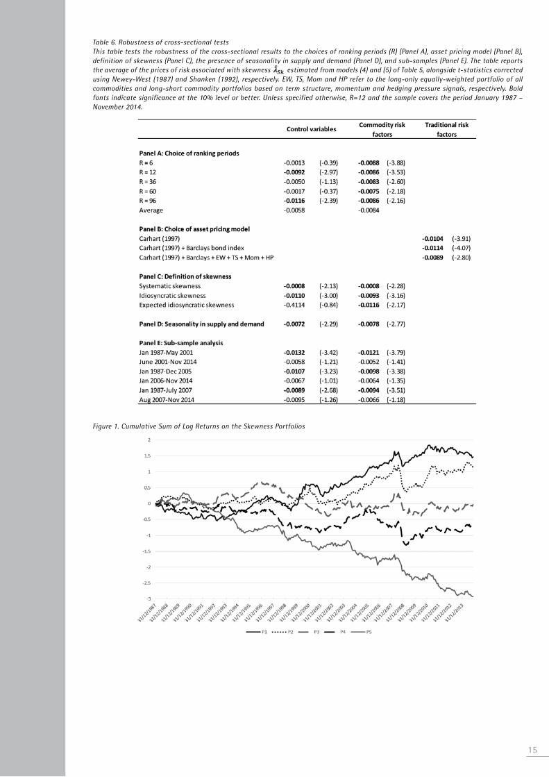
Table 6. Robustness of cross-sectional testsThis table tests the robustness of the cross-sectional results to the choices of ranking periods (R) (Panel A), asset pricing model (Panel B), definition of skewness (Panel C), the presence of seasonality in supply and demand (Panel D), and sub-samples (Panel E). The table reports the average of the prices of risk associated with skewness estimated from models (4) and (5) of Table 5, alongside t-statistics corrected using Newey-West (1987) and Shanken (1992), respectively. EW, TS, Mom and HP refer to the long-only equally-weighted portfolio of all commodities and long-short commodity portfolios based on term structure, momentum and hedging pressure signals, respectively. Bold fonts indicate significance at the 10% level or better. Unless specified otherwise, R=12 and the sample covers the period January 1987 – November 2014.

Figure 1. Cumulative Sum of Log Returns on the Skewness Portfolios

15

16

References• Adrian, T. and J. Rosenberg. (2008). Stock returns and volatility: Pricing the short-run and long-run components of volatility risk, Journal of Finance 63, 2997-3030.

• Amaya, D., P. Christoffersen, K. Jacobs, and A. Vasquez. (2015). Does realised skewness predict the cross-section of equity returns?, Journal of Financial Economics forthcoming.

• Ang, A., R. J. Hodrick, Y. Xing, and X. Zhang. (2006). The cross-section of volatility and expected returns. Journal of Finance 61, 259-299.

• Ang, A., R. J. Hodrick, Y. Xing, and X. Zhang. (2009). High idiosyncratic volatility and low returns: International and further U.S. evidence, Journal of Financial Economics 91, 1–23.

• Bakshi, G., X. Gao, and A. Rossi. (2015). A better specified asset pricing model to explain the cross-section and time-series of commodity returns. Unpublished Working Paper, University of Maryland.

• Bali, T. G., N. Caciki, and R. F. Whitelaw. (2011). Maxing out: Stocks as lotteries and the cross-section of expected returns, Journal of Financial Economics 99, 427–446

• Bali, T. G., and S. Murray. (2013). Does risk-neutral skewness predict the cross section of equity option portfolio returns?, Journal of Financial and Quantitative Analysis 48, 1145-1171.

• Barberis, N., and M. Huang. (2008). Stocks as lotteries: The Implications of probability weighting for security prices. American Economic Review 98, 2066–2100.

• Basu, D., and J. Miffre. (2013). Capturing the risk premium of commodity futures: The role of hedging pressure, Journal of Banking and Finance 37, 2652-2664.

• Bessembinder, H. (1992). Systematic risk, hedging pressure, and risk premiums in futures markets, Review of Financial Studies 5, 637-667.

• Boyer, B., T. Mitton, and K. Vorkink. (2010). Expected idiosyncratic skewness, Review of Financial Studies 23, 169-202.

• Boyer, B., and K. Vorkink. (2014). Stock options as lotteries, Journal of Finance 64, 1485-1527.

• Brennan, M. (1958). The supply of storage, American Economic Review 48, 50-72.

• Brunnermeier, M. (2009). Deciphering the liquidity and credit crunch 2007-2008. Journal of Economic Perspectives, 23, 77-100.

• Brunnermeier, M., C. Gollier, and J. Parker (2007). Optimal beliefs, asset prices, and the preference for skewed returns. American Economic Review, 97, 159-165.

• Carhart, M. (1997). On persistence of mutual fund performance. Journal of Finance 52, 57-82.

• Chang, E., 1985, Return to Speculators and the Theory of Normal Backwardation, Journal of Finance, 40, 193-208.

• Chang, B. Y., P. Christoffersen, and K. Jacobs. (2013). Market skewness risk and the cross section of stock returns, Journal of Financial Economics 107, 46–68.

• Conrad, J., R. Dittmar, and E. Ghysels. (2012). Ex-ante skewness and expected stock returns, Journal of Finance 68, 85-124.

• Cootner, P. (1960). Returns to speculators: Telser vs. Keynes. Journal of Political Economy 68, 396–404.

• Deaton, A., and G. Laroque. (1992) On the behaviour of commodity prices, Review of Economic Studies 59, 1-23.

• Dewally, M., L. Ederington, and C. Fernando. (2013). Determinants of trader profits in commodity futures markets. Review of Financial Studies 26, 2648-2683.

• Erb, C., and C. Harvey. (2006). The strategic and tactical value of commodity futures, Financial Analysts Journal 62, 69-97.

• Fama, E. F., and J. D. MacBeth. (1973). Risk, returns, and equilibrium: Empirical tests, Journal of Political Economy 81, 607-636.

• Fama, E., and K. French. (1987). Commodity futures prices: Some evidence on forecast power, premiums, and the theory of storage, Journal of Business 60, 55-73.

• Gorton, G., F. Hayashi, and G. Rouwenhorst. (2012). The fundamentals of commodity futures returns, Review of Finance 17, 35-105.

• Gorton, G., and G. Rouwenhorst. (2006). Facts and fantasies about commodity futures, Financial Analysts Journal 62, 47-68.

• Harvey, C. R., and A. Siddique. (2000). Conditional skewness in asset pricing tests, Journal of Finance 55, 1263– 95.

• Hirshleifer, D. (1988). Residual risk, trading costs, and commodity futures risk premia, Review of Financial Studies, 1, 173-193.

• Kaldor, N. (1939) Speculation and economic stability, Review of Economic Studies 7, 1-27.

• Keynes, M. (1930). A treatise on money, II: The applied theory of money. Edition Macmillan and Co.

• Kraus, A., and R. H. Litzenberger. (1976). Skewness preference and the valuation of risky assets, Journal of Finance 31, 1085–100.

• Kumar, A. (2009). Who gambles in the stock market?, Journal of Finance 64, 1889-1933.

• Locke, P., and P. Venkatesh. (1997). Futures market transaction costs, Journal of Futures Markets 17, 229-245.

• Miffre, J., and G. Rallis. (2007). Momentum strategies in commodity futures markets, Journal of Banking and Finance 31, 6, 1863-1886.

• Mitton, T., and K. Vorkink. (2007). Equilibrium underdiversification and the preference for skewness, Review of Financial Studies 20, 1255-1288.

• Newey, W. K., and West, K. D. (1987) Hypothesis testing with efficient method of moments estimation, International Economic Review 28, 777-787.

• Shanken, J. (1992). On the estimation of beta-pricing models, Review of Financial Studies 5, 1–33.

• Stoll, H., and R. Whaley. (2010). Commodity index investing and commodity futures prices, Journal of Applied Finance 20, 7–46.

• Symeonidis, L., M. Prokopczuk, C. Brooks, E. Lazar. (2012). Futures basis, inventory and commodity price volatility: An empirical analysis, Economic Modelling 29, 2651-2663.

• Working, H. (1949). The theory of price of storage, American Economic Review 39, 1254-1262.

17

Founded in 1906, EDHEC Business School offers management education at undergraduate, graduate, post-graduate and executive levels. Holding the AACSB, AMBA and EQUIS accreditations and regularly ranked among Europe’s leading institutions, EDHEC Business School delivers degree courses to over 6,000 students from the world over and trains 5,500 professionals yearly through executive courses and research events. The School’s ‘Research for Business’ policy focuses on issues that correspond to genuine industry and community expectations.

Established in 2001, EDHEC-Risk Institute has become the premier academic centre for industry-relevant financial research. In partnership with large financial institutions, its team of ninety permanent professors, engineers, and support staff, and forty-eight

research associates and affiliate professors, implements six research programmes and sixteen research chairs and strategic research projects focusing on asset allocation and risk management. EDHEC-Risk Institute also has highly significant executive education activities for professionals.

In 2012, EDHEC-Risk Institute signed two strategic partnership agreements with the Operations Research and Financial Engineering department of Princeton University to set up a joint research programme in the area of risk and investment management, and with Yale School of Management to set up joint certified executive training courses in North America and Europe in the area of investment management.

Copyright © 2015 EDHEC-Risk Institute

EDHEC-Risk Institute393 promenade des AnglaisBP 3116 - 06202 Nice Cedex 3FranceTel: +33 (0)4 93 18 78 24

EDHEC Risk Institute—Europe 10 Fleet Place, LudgateLondon EC4M 7RBUnited KingdomTel: +44 207 871 6740

www.edhec-risk.com

EDHEC Risk Institute—Asia1 George Street#07-02Singapore 049145Tel: +65 6438 0030

EDHEC Risk Institute—France 16-18 rue du 4 septembre75002 Paris FranceTel: +33 (0)1 53 32 76 30

For more information, please contact: Carolyn Essid on +33 493 187 824 or by e-mail to: carolyn.essid@edhec-risk.com