Commodity futures and market efficiency

Ladislav Kristoufeka,b, Miloslav Vosvrdaa,b

aInstitute of Information Theory and Automation, Academy of Sciences of the Czech Republic, PodVodarenskou Vezi 4, 182 08, Prague, Czech Republic, EU

bInstitute of Economic Studies, Faculty of Social Sciences, Charles University in Prague, Opletalova 26,110 00, Prague, Czech Republic, EU

Abstract

We analyze the market efficiency of 25 commodity futures across various groups – metals,energies, softs, grains and other agricultural commodities. To do so, we utilize recentlyproposed Efficiency Index to find that the most efficient of all the analyzed commoditiesis heating oil, closely followed by WTI crude oil, cotton, wheat and coffee. On the otherend of the ranking, we detect live cattle and feeder cattle. The efficiency is also foundto be characteristic for specific groups of commodities – energy commodities being themost efficient and the other agricultural commodities (formed mainly of livestock) theleast efficient groups. We also discuss contributions of the long-term memory, fractaldimension and approximate entropy to the total inefficiency. Last but not least, we comeacross the nonstandard relationship between the fractal dimension and Hurst exponent.For the analyzed dataset, the relationship between these two is positive meaning that localpersistence (trending) is connected to global anti-persistence. We attribute this to specificsof commodity futures which might be predictable in a short term and locally but in a longterm, they return to their fundamental price.

Keywords: commodities, efficiency, entropy, long-term memory, fractal dimensionJEL codes: C10, G14

Email addresses: kristouf@utia.cas.cz (Ladislav Kristoufek), vosvrda@utia.cas.cz (MiloslavVosvrda)

Preprint submitted to Energy Economics September 9, 2013

arX

iv:1

309.

1492

v1 [

q-fi

n.ST

] 5

Sep

201

3

1. Introduction

Efficient markets hypothesis (EMH) has been a cornerstone of financial economics fordecades and it has been brought to the centre by the influential paper of Fama (1970)summarizing empirical findings following the idea of the efficient markets hypothesis byFama (1965) and Samuelson (1965). Even though the actual definitions differ, the formerstudy builds on a random walk definition and the latter one on a martingale definition, thequalitative consequences are the same – the efficiency of a market originates in impossibil-ity of systematic beating of the market, usually in a form of above-average risk-adjustedreturns. Fama (1991) later separated the efficiency hypothesis into three forms – weak,medium and strong – which differ by different information sets taken into consideration andall are based on inclusion of the information sets in market prices. The weak-form EMHsays that all past price movements (and associated statistics) are already reflected in themarket prices. Prediction of market movements based on historical time series (technicalanalysis) is thus not possible for this form. The medium-form EMH states that all publiclyavailable information are already contained in the prices, the strong-form EMH adds all(even privately) available information. The medium-form thus discards fundamental anal-ysis as well and the strong-form eliminates even insiders from making profit. Evidently, aweaker form of EMH is always a subset of a stronger form. Even though EMH has beenrepeatedly disparaged both empirically and theoretically (Cont, 2001; Malkiel, 2003), andeven more so after an outbreak of the Global Financial Crisis in 2007/2008, its validityremains an open issue, yet still it persists in standard textbooks of financial economics(Elton et al., 2003).

Comparison of efficiency across various assets has been discussed in different studies.In a series of papers, Di Matteo et al. (2003, 2005) and Di Matteo (2007) study long-term memory and multi-scaling of a wide portfolio of stock indices, foreign exchange rates,Treasury rates and Eurodollar interbank interest rates using various estimators of long-termmemory. They show that stock indices of more developed countries are also more efficientyet showing a weak signs of anti-persistence (properties of long-term memory are describedin detail in the Methodology section), finding no deviations from EMH for all analyzedmaturities of Eurodollar and Treasury rates. For US dollar exchange rates, the authorsfind diverse results with no evident pattern connecting exchange rate efficiency level withgeographical or geopolitical properties. In another series of papers, Cajueiro and Tabak(2004a,b,c, 2005) compare stock market indices from different continents finding that theUS and Japanese markets are the most efficient ones whereas the Asian and Latin Americanones are detected as the least efficient ones. Lim (2007) studies non-linear dependencies,their evolution in time and connection to market efficiency for a set of stock markets.The author finds the US market to be the most efficient one followed by Korea, Taiwanand Japan. On the other end of the ranking, Malaysia, Chile and Argentina are placed.Zunino et al. (2010) utilize the complexity-entropy causality plane to rank stock marketindices to show that the emergent markets are less efficient than the developed ones as onewould expect. The difference is attributed to a lower entropy and a higher complexity ofthe emergent markets. Kristoufek and Vosvrda (2013) introduce the Efficiency Index and

2

come up with a ranking of stock market indices finding that the most efficient markets arelocated in Western Europe, USA and Japan whereas the least efficient markets are situatedin Latin America and Asia.

However, up to our best knowledge, proper attention has not been given to a comparisonof the efficiency of commodity markets. In this paper, we analyze futures markets for a widerange of commodities – energy, metals and various agricultural commodities – and comparetheir efficiency using the Efficiency Index proposed by Kristoufek and Vosvrda (2013).The paper is structured as follows. Section 2 covers literature dealing with the efficiencyof commodities. Section 3 describes the methodology in detail. Section 4 describes theanalyzed dataset and brings the results. Section 5 concludes. We show that efficiency isrelated to a type of commodity (energy commodities being the most efficient ones and otheragricultural commodities being the least efficient ones). In addition, we find a nonstandardrelationship between the local and global properties of the series as most of the series showlocal persistence while in global, they are mean-reverting. The series thus follow quitestrong local trends but in a long term, they return to their fundamental value.

2. Literature review

Testing the market efficiency in commodities markets has a long history. Roll (1972)examines the commodity price index and argues that the market is inefficient due to sig-nificant serial correlations of its returns. Danthine (1977) disputes such claim and showsthat the violation of the standard martingale condition does not imply inefficiency in thecommodity spot markets with support of risk aversion and no arbitrage opportunities.Gjolberg (1985) analyzes oil spot prices at the Rotterdam market, rejects the efficiencyhypothesis and constructs a profitable trading rule for daily, weekly and monthly pricechanges. Panas (1991) studies the Rotterdam oil market as well together with the Italianmarket and based on leptokurtic monthly price changes, he rejects the markets’ efficiency.Herbert and Kreil (1996) examine the US spot (cash) and futures markets for natural gasand find these to be inefficient. They argue that such inefficiency is caused by the specificstructure of the US gas markets.

More recently, Tabak and Cajueiro (2007) analyze the efficiency of Brent and WTIcrude oil using the rescaled range analysis and show that the markets are becoming moreefficient in time. Alvarez-Ramirez et al. (2008) study the auto-correlation structure of thecrude oil process using the detrended fluctuation analysis. They show that in long-term,the market is efficient but in short-term, the auto-correlation structure leads to rejectionof the efficiency. Alvarez-Ramirez et al. (2010) further inspect the crude oil markets usinglagged detrended fluctuation analysis and argue that multi-scaling and deviations from therandom walk behavior cause the spot prices to be inefficient. The research on evolutionof efficiency in time is further extended by Wang and Liu (2010) where the authors studyshort-, medium- and long-term efficiency for various scales of the detrended fluctuationanalysis approach. They show that the WTI crude oil becomes more efficient in time forall three analyzed scales. Using also the detrended fluctuation analysis, Wang et al. (2011)argue that WTI crude oil spot and futures are not efficient for short time scales below one

3

month. Crude oil markets (Brent and WTI) are also analyzed by Charles and Darne (2009)who use the variance ratio tests to show that the Brent market is weak-form efficient butthe WTI market is not while providing some discussion about effects of deregulation onthe markets.

Lee and Lee (2009) study four energy commodities – coal, oil, gas and electricity – usingpanel data stationarity tests to uncover that none of the studied markets is efficient in thestrict stationarity sense. Lean et al. (2010) study WTI crude oil spot and futures pricesusing mean-variance and stochastic dominance approaches finding no arbitrage opportuni-ties between spot and futures prices while the findings are robust for various sub-periodsand critical events. Narayan et al. (2010) study long-term relationship between spot andfutures prices of gold and oil. They find that investors use the gold market to hedge againstinflation and for our purposes also more importantly that crude oil market predicts thegold market and vice versa implying inefficiency.

Wang and Yang (2010) study high-frequency futures data of crude oil, heating oil,gasoline and natural gas using various nonlinear models. For heating oil and natural gas,the authors find market inefficiencies which are profound mainly during the bull marketconditions. Gebre-Mariam (2011) focuses on the US natural gas market (spot and futures)finding no arbitrage opportunities for daily prices but in general, the author claims thatthe markets can be seen as efficient only for contracts with approximately a month tomaturity. Martina et al. (2011) utilize entropy approaches to WTI crude oil spot pricesand find various cycles in its prices. Entropy is also applied by Ortiz-Cruz et al. (2012)who again study daily WTI prices finding the market to be efficient with two episodes ofinefficiency connected to the early 1990s and late 2000s US recessions. The authors stressthat deregulation of the market has helped improving its efficiency.

Zunino et al. (2011) apply information theory methods (specifically the permutationentropy and permutation statistical complexity) to the commodity markets allowing themfor efficiency ranking finding silver, copper and cotton to be the most efficient commodi-ties. Wang et al. (2011) study the gold market using the multifractal detrended fluctuationanalysis to show that the market becomes more efficient in time especially after 2001. Kimet al. (2011) use the random matrix theory and network analysis to show that stock andcommodity markets are well decoupled except for oil and gold showing signs of inefficiency.Kim et al. (2011) then focus on the Korean agricultural market using the detrended fluc-tuation analysis finding anti-correlated series with strong volatility clustering aiming atinefficiency.

Out of these selected papers, it is evident that analysis of efficiency of commoditymarkets is fruitful with many approaches to the topic. However, the studies usually focus ona single (or a pair) of efficiency measures to test whether the specific markets are or are notefficient. Moreover, the analysis is usually strongly focused on a single commodity or a smallgroup of commodities. Here, we contribute to the literature by applying various efficiencymeasures on a wide portfolio of commodities ranging from energy and agricultural (withseveral subgroups) commodities to metals. Moreover, we utilize the efficiency measureintroduced by Kristoufek and Vosvrda (2013) to rank the commodities according to theirefficiency.

4

3. Methodology

Efficient market can be defined in several ways. The main distinction roots back to1965 when Fama (1965) and Samuelson (1965) used different definitions – a random walkand a martingale, respectively. We stick to the martingale definition efficiency because itis less restrictive. Based on this definition, we assume that the returns of a financial assetare serially uncorrelated and with finite variance for the efficient market situation. Such asimple definition allows to use various measures of market efficiency, which are describedin this section. Eventually, we refer to the Efficient Index which takes these statistics intoconsideration and it helps to rank different assets according to their efficiency while usingvarious dynamic properties of the time series under study.

3.1. Long-term memory

Long-term memory (long-range dependence) series are characteristic with values in(even distant, in theory infinitely distant) past influencing the present and future values.These processes are standardly described with the long-term memory parameter H (Hurstexponent) which ranges between 0 ≤ H < 1 for stationary invertible processes. Themidpoint, H = 0.5, holds for uncorrelated (or in general short-term memory) processes, i.e.processes of the efficient market. For H > 0.5, the processes are positively correlated withlong-term memory and are usually referred to as persistent. These processes systematicallyfollow local trends while still remaining stationary. ForH < 0.5, we have long-term memoryprocesses with negative correlations – anti-persistent processes. Such processes switch thedirection more often than a random process does.

More formally, the long-term memory processes are defined in both time and frequencydomains. In the time domain, it is connected to a power-law decaying auto-correlationfunction. For the auto-correlation function ρ(k) with time lag k, the decay is characterizedas ρ(k) ∝ k2H−2 for k → +∞. In the frequency domain, the spectrum f(λ) with frequencyλ of the long-range dependent process diverges at the origin so that f(λ) ∝ λ1−2H forλ → 0+. These definitions further lead to non-summable auto-correlations and divergingcovariance of partial sums of the process for the persistent series. These properties are usedin various estimators of parameter H. For comparison of both time and frequency domainestimators, see Beran (1994); Taqqu et al. (1995); Taqqu and Teverovsky (1996); Robinson(1995); Geweke and Porter-Hudak (1983); Di Matteo et al. (2003); Di Matteo (2007);Barunik and Kristoufek (2010); Teverovsky et al. (1999). Out of theses estimators, we optfor the local Whittle and GPH estimators which are suitable for short time series with apossible weak short-term memory (Taqqu et al., 1995; Taqqu and Teverovsky, 1996), whichcan easily bias the time domain estimators (Teverovsky et al., 1999; Kristoufek, 2012).Moreover, these estimators have well-defined asymptotic properties – they are consistentand asymptotically normal estimators.

Local Whittle estimator

The local Whittle estimator (Robinson, 1995) is a semi-parametric maximum likelihoodestimator utilizing a likelihood function of Kunsch (1987) and focusing only on a part of

5

the spectrum f(λ) near the origin. The full parametric specification is thus not neededand one does not need to assume any specific underlying long-term memory model butonly a model with divergent at origin spectrum. This way, the estimator does not takeinto consideration high frequencies and it is in turn resistant to the short-term memorybias. As an estimator of the spectrum of series {xt}, we use the periodogram defined asI(λj) = 1

T

∑Tt=1 exp(−2πitλj)xt with j = 1, 2, . . . ,m where m ≤ T/2 and λj = 2πj/T .

The local Whittle estimator is defined as

H = arg min0≤H<1

R(H), (1)

where

R(H) = log

(1

m

m∑j=1

λ2H−1j I(λj)

)− 2H − 1

m

m∑j=1

log λj. (2)

The local Whittle estimator is consistent and asymptotically normal, specifically√m(H −H0)→d N(0, 1/4). (3)

GPH estimator

Contrarily to the local Whittle estimator, the GPH estimator, named after the authorsof Geweke and Porter-Hudak (1983), is based on a full functional specification of theunderlying process as the fractional Gaussian noise implying a specific spectral form:

log f(λ) ∝ −(H − 0.5) log(4 sin2(λ/2)) (4)

Again, the spectrum is estimated using the periodogram and the Hurst exponent is esti-mated using the ordinary least squares on

log I(λj) ∝ −(H − 0.5) log(4 sin2(λj/2)). (5)

The GPH estimator is consistent and asymptotically normal (Beran, 1994), specifically√T (H −H0)→d N(0, π2/6). (6)

The GPH estimator is thus asymptotically infinitely more efficient than the local Whit-tle estimator. However, this is true only if the true underlying process is in fact thefractional Gaussian noise. In financial and economic time series, this is frequently not thecase as the processes are mostly a combination of short-term (such us autoregressive mov-ing average – ARMA – processes of various specifications) and long-term memory (such asthe aforementioned fractional Gaussian noise of fractionally integrated ARMA) processes.In this case, the GPH estimator becomes biased. To avoid the bias, the GPH estima-tor is based only on a part of the spectrum (periodogram) close to the origin as for thelocal Whittle estimator. The regression in Eq. 5 is then applied only for a part of theperiodogram based on the same parameter m as for the local Whittle estimator1.

1In our analysis, we apply m = T 0.6 (Phillips and Shimotsu, 2004).

6

3.2. Fractal dimension

Contrary to the long-term memory, which can be seen as a characteristic of globaldependence and correlation structure, the fractal dimension D can be taken as a measureof local memory of the series as it is a measure of roughness of the series (Kristoufek andVosvrda, 2013). As the series can be differently rough or smooth for its specific parts,it can be locally serially correlated even though on a global level, the correlations mightvanish and are not necessarily observable or detectable.

For a univariate series, the fractal dimension ranges between 1 < D ≤ 2. For self-similarprocesses, the fractal dimension is tightly connected to the Hurst exponent (long-termmemory) of the series so that D = 2−H. In economic terms, this can be understood as aperfect transmission of a local behavior (fractal dimension) to a global behavior (long-termmemory). However, the relation usually does not hold perfectly for the financial series sothat both D and H give different insights into the dynamics of the series making it worthstudying them separately.

In general, D = 1.5 holds for an uncorrelated series with no local trending or no localanti-correlations and thus it is also a value of D for the efficient market. For a low fractaldimension D < 1.5, the roughness of the series is lower than for an uncorrelated processso that we observe local trending and the series is said to be locally persistent. Reversely,a high fractal dimension D > 1.5 characterizes a series rougher than the uncorrelated one,which is connected to local anti-persistence, i.e. the series are negatively auto-correlatedlocally. For purposes of the Efficiency Index introduced later in this section, we utilizeHall-Wood and Genton estimators (Gneiting and Schlather, 2004; Gneiting et al., 2010).

Hall-Wood estimator

Hall-Wood estimator (Hall and Wood, 1993) is a box-counting procedure which utilizesscaling of absolute deviations between steps. Formally, we have

A(l/n) =

⌊l

n

⌋ bn/lc∑i=1

|xibl/nc − x(i−1)bl/nc| (7)

representing the absolute deviations. Using the definition of the fractal dimension (Gneitingand Schlather, 2004; Gneiting et al., 2010), the Hall-Wood estimator is given by

DHW = 2−∑L

l=1 (sl − s) log(A(l/n))∑Ll=1 (sl − s)2

(8)

where L ≥ 2, sl = log(l/n) and s = 1L

∑Ll=1 sl. To minimize potential bias, Hall and Wood

(1993) propose using L = 2 so that we obtain the estimate of the fractal dimension DHW

as

DHW = 2− log A(2/n)− log A(1/n)

log 2. (9)

7

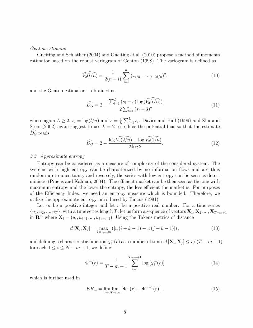
Genton estimator

Gneiting and Schlather (2004) and Gneiting et al. (2010) propose a method of momentsestimator based on the robust variogram of Genton (1998). The variogram is defined as

V2(l/n) =1

2(n− l)

n∑i=l

(xi/n − x(i−l)l/n)2, (10)

and the Genton estimator is obtained as

DG = 2−∑L

l=1 (sl − s) log(V2(l/n))

2∑L

l=1 (sl − s)2(11)

where again L ≥ 2, sl = log(l/n) and s = 1L

∑Ll=1 sl. Davies and Hall (1999) and Zhu and

Stein (2002) again suggest to use L = 2 to reduce the potential bias so that the estimate

DG reads

DG = 2− log V2(2/n)− log V2(1/n)

2 log 2. (12)

3.3. Approximate entropy

Entropy can be considered as a measure of complexity of the considered system. Thesystems with high entropy can be characterized by no information flows and are thusrandom up to uncertainty and reversely, the series with low entropy can be seen as deter-ministic (Pincus and Kalman, 2004). The efficient market can be then seen as the one withmaximum entropy and the lower the entropy, the less efficient the market is. For purposesof the Efficiency Index, we need an entropy measure which is bounded. Therefore, weutilize the approximate entropy introduced by Pincus (1991).

Let m be a positive integer and let r be a positive real number. For a time series{u1, u2, ..., uT}, with a time series length T , let us form a sequence of vectors X1,X2, ...,XT−m+1

in Rm where Xi = (ui, ui+1, ..., ui+m−1). Using the Takens metrics of distance

d [Xi,Xj] = maxk=1,...,m

(|u (i+ k − 1)− u (j + k − 1)|) , (13)

and defining a characteristic function χmi (r) as a number of times d [Xi,Xj] ≤ r/ (T −m+ 1)

for each 1 ≤ i ≤ N −m+ 1, we define

Φm(r) =1

T −m+ 1

T−m+1∑i=1

log [χmi (r)] (14)

which is further used in

ERm = limr→0

limT→∞

[Φm(r)− Φm+1(r)

]. (15)

8

The approximate entropy (ApEn) is then defined as

ApEn = limm→∞

ERm. (16)

Since r can be seen as an discriminating factor for the distance measured by the Takensmetrics and m is the number of elements whose closeness is measured, the approximateentropy measures whether different segments of the series follow similar patterns. For anidentically uniformly independently distributed random process, the approximate entropyconverges to − log

(r/√

3)

for all m (Pincus, 1991). For a completely deterministic process,the entropy goes to 0. Therefore, we can rescale the approximate entropy so that 0 ≤ApEn ≤ 1, where 0 characterizes a completely deterministic process and 1 a completelyuncertain process characteristic for the efficient market. In turn, it can be utilized in theEfficiency Index, definition of which follows.

3.4. Capital market efficiency measure

Kristoufek and Vosvrda (2013) introduce the Efficiency Index (EI) is defined as

EI =

√√√√ n∑i=1

(Mi −M∗

i

Ri

)2

, (17)

where Mi is the ith measure of efficiency, Mi is an estimate of the ith measure, M∗i is

an expected value of the ith measure for the efficient market and Ri is a range of the ithmeasure. In words, EI is simply a distance from the efficient market situation. Here,we base the index on three measures of market efficiency – Hurst exponent H with anexpected value of 0.5 for the efficient market (M∗

H = 0.5), fractal dimension D with anexpected value of 1.5 (M∗

D = 1.5) and the approximate entropy with an expected value of1 (M∗

AE = 1). Hurst exponent is taken as an average of the GPH and the local Whittleestimates. In the same way, the fractal dimension is set as an average of the Hall-Wood andGenton estimates. For the approximate entropy, we utilize the estimate described in thecorresponding section. The approximate entropy need to be rescaled as it ranges between0 and 1 with the efficient market of ApEn = 1. We thus have RAE = 2 and RD = RH = 1.

4. Data description and results

We analyze daily front futures prices, i.e. futures with the earliest delivery, of 25 com-modities in period between 1.1.2000 and 22.7.20132. The dataset contains 4 energy (Brentcrude oil, WTI crude oil, heating oil and natural gas), 5 metals (copper, gold, silver, palla-dium and platinum), 7 grains (corn, oats, rough rice, soybean meal, soybean oil, soybeansand wheat), 5 softs (cocoa, coffee, cotton, orange juice and sugar) and 4 other agricul-tural commodities (feeder cattle, lean hogs, live cattle and lumber) futures from Chicago

2The time series were obtained from http://www.quandl.com server on 23.7.2013.

9

Board of Trade (CBOT), Chicago Mercantile Exchange (CME), IntercontinentalExchange(ICE), New York Mercantile Exchange (NYMEX) and its division Commodity Exchange(COMEX), which are summarized in Tab. 1. We analyze logarithmic prices Si,t = logPi,t,where Pi,t is the price of futures i at time t, for the fractal dimension and logarithmicreturns ri,t = Si,t−Si,t−1 for the long-term memory and approximate entropy. The returnsof all the analyzed futures are stationary according to ADF (Dickey and Fuller, 1979) andKPSS (Kwiatkowski et al., 1992) tests (we do not report the p-values here).

Estimated Hurst exponents, fractal dimensions and approximate entropies are sum-marized in Tab. 2. We observe that majority of commodities is characteristic with thefractal dimension below 1.5 which indicates local persistence. These series are thus locallytrending. This is most evident for feeder cattle, lean hogs and live cattle, i.e. majorlylivestock futures. On the contrary, the energy commodities – namely both the crude oilsand natural gas – are close to fractal dimension of 1.5 and as such, they do not show anysigns of local inefficiencies. For the long-term memory part, most of the futures are below0.5 indicating anti-persistence which translates into a mean-reversion of prices, somethingthat is not standardly observed for stocks, stock indices and exchange rates which arecharacteristic by a unit-root behavior. The strongest anti-persistence is seen for cocoa,oats and orange juice. Nonetheless, there is a portion of commodities which show signsof persistence. These are copper, palladium, platinum and sugar. Cotton and natural gasget the closest to the value of the efficient market. For the approximate entropy, severalvalues are close to 1 for the efficient market3 – lumber, sugar and heating oil. The mostcomplex, and thus the least efficient, series include feeder cattle and live cattle.

Putting these results together, we arrive at the Efficiency Indices and efficiency rankingwhich are graphically represented in Fig. 1. The most efficient of the commodities turnsout to be heating oil closely followed by WTI crude oil. Cotton, wheat and coffee comeafter these with a similar level of efficiency. The ranking is then supplemented by othercommodities, efficiency of which increases quite steadily across the ranking. Feeder cattle isthe least efficient commodity in this set quite closely followed by live cattle. The livestockfutures thus seem to be rather inefficient compared to the others. Connected to this finding,we also show an average Efficiency Index for commodities according to their type. In Fig.2, we can see that the energy futures are the most efficient ones followed by softs, grains andmetals. By far the least efficient group consists of the other agricultural commodities, i.e.feeder cattle, lean hogs, live cattle and lumber. This is well in hand with the observationsabout very inefficient livestock futures.

In Figs. 3 and 4, we decompose the efficiency index into its parts. In Fig. 3, the actualfutures ranked according to the Efficiency Index are represented, and in Fig. 4, these aresorted according to their type to better see possible patterns and regularities. We observethat for about half of the futures, the approximate entropy is the dominant inefficiencysource. Interestingly, it is the most important part for both the most and the least efficientcommodities. For the others, the long-term memory part is dominant. Fractal dimension

3Several values even reach value above 1 due to the finite sample.

10

forms usually only a smaller part of the inefficiency and only for wheat, it contributesthe most. When we look at the whole groups of commodities, we observe that for energy,grains and other agricultural commodities, the approximate entropy forms an important oreven a dominant part for most of them. For grains, fractal dimension creates a significantpart for three of the group. For softs, the long-term memory is the most important of theinefficiency contributors. And for metals, the evidence is mixed.

Fig. 5 then illustrates a relationship between fractal dimension and Hurst exponent.For self-similar processes, it holds that D = 2 − H. In economic terms, self-similar pro-cesses are characteristic by translating the local properties into the global ones. Therefore,for a locally persistent process with D < 1.5, this translates into the global persistencewith H > 0.5, and vice versa. However, we do not observe such relationship for the ana-lyzed commodities. Actually, the dependence is reversed so that with the increasing Hurstexponent, the fractal dimension increases. This is in contrast with the results for stockindices (Kristoufek and Vosvrda, 2013). Nonetheless, such result can be well explainedby characteristics of commodities futures – locally (or in the short term), the changes infutures prices are partially predictable, but globally, the prices return to their fundamentalvalues.

5. Conclusion

We have analyzed the market efficiency of 25 commodities futures across various groups– metals, energies, softs, grains and other agricultural commodities. To do so, we haveutilized the recently proposed Efficiency Index to find that the most efficient of all theanalyzed commodities is heating oil, closely followed by WTI crude oil, cotton, wheatand coffee. On the other end of the ranking, we have detected live cattle and feedercattle. The efficiency also seems to be characteristic for specific groups of commodities –energy commodities have been found the most efficient, followed by softs, grains and metalswhereas the other agricultural commodities (formed mainly of livestock) form the leastefficient group. Apart from that, we have also discussed the contributions of the long-termmemory, fractal dimension and approximate entropy to the total inefficiency. We haveuncovered that the contribution is type-dependent as well even though the regularitiesare not strongly pronounced. Last but not least, we have come across the nonstandardrelationship between the fractal dimension and Hurst exponent. For the analyzed dataset,the relationship between these two is positive meaning that local persistence (trending) isconnected to global anti-persistence. We attribute this to specifics of commodity futureswhich might be predictable in a short term and locally but in a long term, they return totheir fundamental price, which differs from the results found for stock indices (Kristoufekand Vosvrda, 2013).

Acknowledgements

The support from the Czech Science Foundation under Grants 402/09/0965 and P402/11/0948,and project SVV 267 504 are gratefully acknowledged.

11

References

References

Alvarez-Ramirez, J., J. Alvarez, and E. Rodriguez (2008). Short-term predictability ofcrude oil markets: A detrended fluctuation analysis approach. Energy Economics 30,2645–2656.

Alvarez-Ramirez, J., J. Alvarez, and R. Solis (2010). Crude oil market efficiency andmodeling: Insights from the multiscaling autocorrelation pattern. Energy Economics 32,993–1000.

Barunik, J. and L. Kristoufek (2010). On Hurst exponent estimation under heavy-taileddistributions. Physica A 389(18), 3844–3855.

Beran, J. (1994). Statistics for Long-Memory Processes, Volume 61 of Monographs onStatistics and Applied Probability. New York: Chapman and Hall.

Cajueiro, D. and B. Tabak (2004a). Evidence of long range dependence in Asian equitymarkets: the role of liquidity and market restrictions. Physica A 342, 656–664.

Cajueiro, D. and B. Tabak (2004b). The Hurst exponent over time: testing the assertionthat emerging markets are becoming more efficient. Physica A 336, 521–537.

Cajueiro, D. and B. Tabak (2004c). Ranking efficiency for emerging markets. Chaos,Solitons and Fractals 22, 349–352.

Cajueiro, D. and B. Tabak (2005). Ranking efficiency for emerging equity markets II.Chaos, Solitons and Fractals 23, 671–675.

Charles, A. and O. Darne (2009). The efficiency of the crude oil markets: Evidence fromvariance ratio tests. Energy Policy 37, 4267–4272.

Cont, R. (2001). Empirical properties of asset returns: stylized facts and statistical issues.Quantitative Finance 1(2), 223 – 236.

Danthine, J.-P. (1977). Martingale, market efficiency and commodity prices. EuropeanEconomic Review 10, 1–17.

Davies, S. and P. Hall (1999). Fractal analysis of surface roughness by using spatial data.Journal of the Royal Statistical Society Series B 61, 3–37.

Di Matteo, T. (2007). Multi-scaling in finance. Quantitatice Finance 7(1), 21–36.

Di Matteo, T., T. Aste, and M. Dacorogna (2003). Scaling behaviors in differently devel-oped markets. Physica A 324, 183–188.

12

Di Matteo, T., T. Aste, and M. Dacorogna (2005). Long-term memories of developed andemerging markets: Using the scaling analysis to characterize their stage of development.Journal of Banking & Finance 29, 827–851.

Dickey, D. and W. Fuller (1979). Distribution of the estimators for autoregressive timeseries with a unit root. Journal of the American Statistical Association 74, 427–431.

Elton, E., M. Gruber, S. Brown, and W. Gotzmann (2003). Modern Portfolio Theory andInvestment Analysis. John Wiley & Sons, Inc., New York.

Fama, E. (1965). The behavior of stock market prices. Journal of Business 38, 34–105.

Fama, E. (1970). Efficient Capital Markets: A Review of Theory and Empirical Work.Journal of Finance 25, 383–417.

Fama, E. (1991). Efficient Capital Markets: II. Journal of Finance 46(5), 1575–1617.

Gebre-Mariam, Y. K. (2011). Testing for unit roots, causality, cointegration, and efficiency:The case of the northwest US natural gas market. Energy 36, 3489–3500.

Genton, M. (1998). Highly robust variogram estimation. Mathematical Geology 30, 213–221.

Geweke, J. and S. Porter-Hudak (1983). The estimation and application of long memorytime series models. Journal of Time Series Analysis 4(4), 221–238.

Gjolberg, O. (1985). Is the spot market for oil products efficient? Some Rotterdam evi-dence. Energy Economics 7(4), 231–236.

Gneiting, T. and M. Schlather (2004). Stochastic Models That Separate Fractal Dimensionand the Hurst Effect. SIAM Review 46(2), 269–282.

Gneiting, T., H. Sevcikova, and D. Percival (2010). Estimators of fractal dimension: As-sessing the roughness of time series and spatial data. Technical report, Department ofStatistics, University of Washington.

Hall, P. and A. Wood (1993). On the performance of box-counting estimators of fractaldimension. Biometrika 80(1), 246–252.

Herbert, J. H. and E. Kreil (1996). US natural gas markets: How efficient are they? EnergyPolicy 24(1), 1–5.

Kim, H., G. Oh, and S. Kim (2011). Multifractal analysis of the Korean agriculturalmarket. Physica A 390, 4286–4292.

Kim, M. J., S. Kim, Y. H. Jo, and S. Y. Kim (2011). Dependence structure of the commod-ity and stock makrets, and relevant multi-spread strategy. Physica A 390, 3842–3854.

13

Kristoufek, L. (2012). How are rescaled range analyses affected by different memory anddistributional properties? A Monte Carlo study. Physica A 391, 4252–4260.

Kristoufek, L. and M. Vosvrda (2013). Measuring capital market efficiency: Global andlocal correlations structure. Physica A 392, 184–193.

Kunsch, H. (1987). Statistical aspects of self-similar processes. Proceedings of the FirstWorld Congress of the Bernoulli Society 1, 67–74.

Kwiatkowski, D., P. Phillips, P. Schmidt, and Y. Shin (1992). Testing the null of station-arity against alternative of a unit root: How sure are we that the economic time serieshave a unit root? Journal of Econometrics 54, 159–178.

Lean, H. H., M. McAleer, and W.-K. Wong (2010). Market efficiency of oil spot andfutures: A mean-variance and stochastic dominance approach. Energy Economics 32,979–986.

Lee, C.-C. and J.-D. Lee (2009). Energy prices, multiple structural breaks, and efficientmarket hypothesis. Applied Energy 86, 466–479.

Lim, K.-P. (2007). Ranking market efficiency for stock markets: A nonlinear perspective.Physica A 376, 445–454.

Malkiel, B. (2003). The efficient market hypothesis and its critics. Journal of EconomicPerspectives 17(1), 5982.

Martina, E., E. Rodriguez, R. Escarela-Perez, and J. Alvarez-Ramirez (2011). Multiscaleentropy analysis of crude oil price dynamics. Energy Economics 33, 936–947.

Narayan, P. K., S. Narayan, and X. Zheng (2010). Gold and oil futures: Are marketsefficient? Applied Energy 87, 3299–3303.

Ortiz-Cruz, A., E. Rodriguez, C. Ibarra-Valdez, and J. Alvarez-Ramirez (2012). Efficiencyof crude oil markets: Evidences from informational entropy analysis. Energy Policy 41,365–373.

Panas, E. (1991). A weak form evaluation of the efficieny of the Rotterdam and Italian oilspot markets. Energy Economics 13(1), 26–32.

Phillips, P. C. B. and K. Shimotsu (2004). Local whittle estimation in nonstationary andunit root cases. The Annals of Statistics 32(2), 659–692.

Pincus, S. (1991). Approximate entropy as a measure of system complexity. Proceedingsof the National Academy of Sciences of the United States of America 88, 2297–2301.

Pincus, S. and R. Kalman (2004). Irregularity, volatility, risk, and financial market timeseries. Proceedings of the National Academy of Sciences of the United States of Amer-ica 101(38), 13709–13714.

14

Robinson, P. (1995). Gaussian semiparametric estimation of long range dependence. TheAnnals of Statistics 23(5), 1630–1661.

Roll, R. (1972). Interest rates on monetary assets and commodity price index changes.Journal of Finance 27(2), 251–277.

Samuelson, P. (1965). Proof that properly anticipated prices fluctuate randomly. IndustrialManagement Review 6, 41–49.

Tabak, B. M. and D. O. Cajueiro (2007). Are the crude oil markets becoming weaklyefficient over time? a test for time-varying long-range dependence in prices and volatility.Energy Economics 29, 28–36.

Taqqu, M., W. Teverosky, and W. Willinger (1995). Estimators for long-range dependence:an empirical study. Fractals 3 (4), 785–798.

Taqqu, M. and V. Teverovsky (1996). On Estimating the Intensity of Long-Range Depen-dence in Finite and Infinite Variance Time Series. In A Practical Guide To Heavy Tails:Statistical Techniques and Applications.

Teverovsky, V., M. Taqqu, and W. Willinger (1999). A critical look at lo’s modified r/sstatistic. Journal of Statistical Planning and Inference 80(1-2), 211–227.

Wang, T. and J. Yang (2010). Nonlinearity and intraday efficiency tests on energy futuresmarkets. Energy Economics 32, 496–503.

Wang, Y. and L. Liu (2010). Is WTI crude oil market becoming weakly efficient over time?new evidence from multiscale analysis based on detrended fluctuation analysis. EnergyEconomics 32, 987–992.

Wang, Y., Y. Wei, and C. Wu (2011). Detrended fluctuation analysis on spot and futuresmarkets of West Texas Intermediate crude oil. Physica A 390, 864–875.

Zhu, Z. and M. Stein (2002). Parameter estimation for fractional brownian surfaces. Sta-tistica Sinica 12, 863–883.

Zunino, L., B. M. Tabak, F. Serinaldi, M. Zanin, D. G. Perez, and O. A. Rosso (2011).Commodity predictability analysis with a permutation information theory approach.Physica A 390, 876–890.

Zunino, L., M. Zanin, B. Tabak, D. Perez, and O. Rosso (2010). Complexity-entropycausality plane: A useful approach to quantify the stock market inefficiency. PhysicaA 389, 1891–1901.

15

Figure 1: Efficiency Index of commodity futures. Commodities are sorted from the most efficientone (left) to the least efficient one (right).

16

Figure 2: Average Efficiency Index for groups of commodities. Groups are sorted from the most(left) to the least (right) efficient ones.

Figure 3: Contribution to inefficiency I. Commodities are sorted according to their efficiency withrespect to Fig. 1.

17

Figure 4: Contribution to inefficiency II. Commodities are sorted according to their group.

Figure 5: Relationship between Hurst exponent and fractal dimension. For self-similar processes,we expect D = 2−H, i.e. a negative slope. The red dashed line represents the least squares fit uncoveringpositive relationship between D and H.

18

Table 1: Analyzed commodities

Full name Short name Type

CBOT Corn C1 Corn GrainsCBOT Oats O1 Oats Grains

CBOT Rough Rice RR1 Rough Rice GrainsCBOT Soybean Meal SM1 Soybean Meal GrainsCBOT Soybean Oil BO1 Soybean Oil Grains

CBOT Soybeans S1 Soybeans GrainsCBOT Wheat W1 Wheat Grains

CME Feeder Cattle FC1 Feeder Cattle Other agriculturalsCME Lean Hogs LN1 Lean Hogs Other agriculturalsCME Live Cattle LC1 Live Cattle Other agriculturals

CME Lumber LB1 Lumber Other agriculturalsCOMEX Copper HG1 Copper MetalsCOMEX Gold GC1 Gold MetalsCOMEX Silver SI1 Silver Metals

ICE Brent Crude Oil B1 Crude Oil (Brent) EnergyICE Cocoa CC1 Cocoa SoftsICE Coffee KC1 Coffee Softs

ICE Cotton No 2 CT1 Cotton SoftsICE Orange Juice OJ1 Orange Juice SoftsICE Sugar No 11 SB1 Sugar Softs

NYMEX Crude Oil CL1 Crude Oil (WTI) EnergyNYMEX Heating Oil HO1 Heating Oil EnergyNYMEX Natural Gas NG1 Natural Gas Energy

NYMEX Palladium PA1 Palladium MetalsNYMEX Platinum PL1 Platinum Metals

19

Table 2: Results

Commodity AE DHW DG HLW HGPH EI

Cocoa 0.9728 1.4665 1.4605 0.3542 0.3367 0.1594Coffee 0.9680 1.4948 1.4606 0.4575 0.4665 0.0469Copper 0.8264 1.5613 1.4974 0.6205 0.6992 0.1843Corn 0.9015 1.4592 1.4299 0.5241 0.4858 0.0744

Cotton 0.9564 1.4702 1.4564 0.5057 0.4735 0.0439Crude Oil (Brent) 0.8919 1.5307 1.5084 0.5620 0.5986 0.0988Crude Oil (WTI) 0.9427 1.5243 1.4987 0.5466 0.4499 0.0309

Feeder Cattle 0.3857 1.3498 1.3166 0.5751 0.3882 0.3500Gold 0.5759 1.5161 1.4707 0.4278 0.4067 0.2277

Heating Oil 0.9568 1.4943 1.4916 0.5081 0.4592 0.0280Lean Hogs 0.7081 1.3894 1.3584 0.3795 0.4256 0.2161Live Cattle 0.4527 1.4206 1.3773 0.4433 0.4306 0.2985

Lumber 1.0040 1.4301 1.4428 0.4278 0.3603 0.1236Natural Gas 1.1140 1.5246 1.4781 0.5210 0.5204 0.0607

Oats 0.9365 1.3926 1.3696 0.4105 0.2364 0.2152Orange Juice 0.8770 1.4266 1.3899 0.4126 0.3399 0.1659

Palladium 1.0230 1.4266 1.4210 0.5625 0.5970 0.1109Platinum 0.7443 1.4686 1.4845 0.5535 0.5465 0.1393

Rough Rice 0.8525 1.4278 1.4181 0.4512 0.4635 0.1149Silver 0.8515 1.5161 1.4914 0.4685 0.4448 0.0861

Soybean Meal 0.8861 1.4448 1.4328 0.4878 0.4548 0.0884Soybean Oil 0.7286 1.4735 1.4364 0.5330 0.5307 0.1465

Soybeans 0.7649 1.4900 1.4745 0.5266 0.5173 0.1209Sugar 0.9759 1.4786 1.4818 0.5543 0.5505 0.0573Wheat 0.9133 1.5129 1.4829 0.4626 0.5117 0.0453

20