commodity payments, farm business survival, and farm size
TRANSCRIPT
Economic Research Report Number 51
November 2007
United States Department of Agriculture
Economic Research Service
Nigel KeyMichael J. Roberts
Commodity Payments,Farm Business Survival,and Farm Size Growth

ww
w.er
s.usda.gov
Visit Our Website To Learn More!
National Agricultural LibraryCataloging Record:
The U.S. Department of Agriculture (USDA) prohibits discrimination in all its programs and activities on the basis of race, color, national origin, age, disability, and, where applicable, sex, marital status, familial status, parental status, religion, sexual orientation, genetic information, political beliefs, reprisal, or because all or a part of an individual's income is derived from any public assistance program. (Not all prohibited bases apply to all programs.) Persons with disabilities who require alternative means for communication of program information (Braille, large print, audiotape, etc.) should contact USDA's TARGET Center at (202) 720-2600 (voice and TDD).
To file a complaint of discrimination write to USDA, Director, Office of Civil Rights, 1400 Independence Avenue, S.W., Washington, D.C. 20250-9410 or call (800) 795-3272 (voice) or (202) 720-6382 (TDD). USDA is an equal opportunity provider and employer.
Cover photo credits: Corbis and CorelProPhoto.
National Agricultural Library Cataloging Record:
Key, Nigel DavidCommodity payments, farm business survival, and farm size growth.(Economic research report (United States. Dept. of Agriculture. Economic Research Service) ; no. 51)
1. Agricultural subsidies—United States. 2. Farms, Size of—Economic aspects—United States. 3. Crops—Economic aspects—United States. I. Roberts, Michael J. (Michael James) II. United States. Dept. of Agriculture. Economic Research Service. III. Title.
HD1470.5.U6
United StatesDepartmentof Agriculture
www.ers.usda.gov
A Report from the Economic Research Service
Nigel Key and Michael J. Roberts
AbstractIn the last 25 years, U.S. crop farms have steadily declined in number and grown in
average size, as production has shifted to larger operations. Larger farms tend to receivemore commodity program payments because most payments are tied to a farm’s currentor historical production, but whether payments have contributed to farm growth isuncertain. This study uses farm-level data from the census of agriculture to determinewhether there is a statistical relationship between farm commodity program paymentsand greater concentration in production. The analysis indicates that, at the regionallevel, higher commodity program payments per acre are associated with subsequentfarm growth. Also, higher payments per acre are associated with higher rates of farmsurvival and growth.
Keywords: agricultural payments, farm size, farm survival, concentration, consolidation,government payments, commodity programs.
AcknowledgmentsThis report benefited from thoughtful and constructive comments provided by JimMacDonald, Mary Bohman, Kitty Smith, Neil Conklin, Keith Wieibe, Pat Sullivan, JoeGlauber, Demcey Johnson, Allen Featherstone, Bill McBride, Allan Gray, and SteveKoenig. We would also like to thank Dale Simms for excellent editorial assistanceand Victor B. Phillips, Jr., for the layout/design.
Economic
Research
Report
Number 51
Commodity Payments,Farm Business Survival,and Farm Size Growth
November 2007
ContentsSummary . . . . . . . . . . . . . . . . . . . . . . . . . . . . . . . . . . . . . . . . . . . . . . . .iii
Chapter 1—Introduction . . . . . . . . . . . . . . . . . . . . . . . . . . . . . . . . . . . .1Perspectives on the Issue . . . . . . . . . . . . . . . . . . . . . . . . . . . . . . . . . .2A New Approach . . . . . . . . . . . . . . . . . . . . . . . . . . . . . . . . . . . . . . . .4
Chapter 2—Determinants of Farm Size and Survival . . . . . . . . . . . .5
Chapter 3—Rapid Growth in Land Concentration . . . . . . . . . . . . . .7Box: Measures of Farmland Concentration . . . . . . . . . . . . . . . . . . .10How Have Commodity Program Payments Changed
Over Time? . . . . . . . . . . . . . . . . . . . . . . . . . . . . . . . . . . . . . . . . . .12
Box: Defining Commodity Program Payments . . . . . . . . . . . . . . . .14
Chapter 4—Commodity Program Payments and the Concentration of Cropland . . . . . . . . . . . . . . . . . . . . . . . . . . . . . .15
Box: ZIP Code Data . . . . . . . . . . . . . . . . . . . . . . . . . . . . . . . . . . . . .16Descriptive Statistics for ZIP Codes . . . . . . . . . . . . . . . . . . . . . . . . .18Land Concentration Change by Payment Category . . . . . . . . . . . . .20
Chapter 5—Effect of Payments on Growth and Survival of Farms . . . . . . . . . . . . . . . . . . . . . . . . . . . . . . . . . .24Payments and Farm Survival . . . . . . . . . . . . . . . . . . . . . . . . . . . . . .24Comparing Survival Rates of Farms With Different Levels of
Program Payments . . . . . . . . . . . . . . . . . . . . . . . . . . . . . . . . . . . .24Box: Measuring the Duration of Farm Business Survival . . . . . . . .25
Controlling for Differences Between Operators and Operations . . .26
Payments and Farm Growth . . . . . . . . . . . . . . . . . . . . . . . . . . . . . . .29
Box: Estimating the Relationship Between Payments and Individual Farm Size . . . . . . . . . . . . . . . . . . . . . . . . . . . . . . . . . . .31
Chapter 6—Summary and Discussion . . . . . . . . . . . . . . . . . . . . . . . .32Have Payments Made Farms Larger? . . . . . . . . . . . . . . . . . . . . . . . .32
References . . . . . . . . . . . . . . . . . . . . . . . . . . . . . . . . . . . . . . . . . . . . . . .34
Appendix: Estimating the Link Between Payments and Concentration Growth . . . . . . . . . . . . . . . . . . . . . . . . . . . . . .38
iiCommodity Payments, Farm Business Survival, and Farm Size Growth / ERR-51
Economic Research Service/USDA
Recommended citation format:
Key, Nigel, and Michael J. Roberts. 2007. Commodity Payments, Farm Business Survival, and Farm Size Growth. U.S. Department of Agriculture,Economic Research Service, ERR-51, November.
Summary
What Is the Issue?
Farm structure is undergoing a complex set of changes. The census of agri-culture shows increasing numbers of small farms (less than 50 acres) andlarge farms (1,000 acres or more), but also sharp and ongoing declines inthe number of farms in the middle. Small farms, while numerous, accountfor less than 2 percent of all U.S. farmland, while large farms account for 67percent. Consequently, the growth in the number of large farms hasincreased the concentration of crop production—that is, an increasinglylarge share of cropland and production is concentrated on relatively fewlarge farms. A number of factors, including technological change orchanging factor prices, could have driven the increase in concentration ofproduction. Commodity program payments may also be contributing to thegrowth in concentration—allowing farms that receive more payments togrow faster than they would have without payments.
This report uses data from five agricultural censuses (1982, 1987, 1992,1997, 2002) to determine whether there is a statistical relationship betweenthe level of commodity program payments received and subsequent changesin farm structure. The analysis pursues four broad questions. How canchanges in concentration of agricultural production be measured and howhas it changed? Is there a link between concentration of agricultural produc-tion, farm size or farm survival, and commodity program payments? If so,how large and how extensive is this link? Finally, what might drive the observed links?
What Did the Study Find?
Crop production is shifting to larger farms. For example, farms with at least1,000 acres in corn harvested 19.8 percent of all U.S. corn acres in 2002, upfrom 4.6 percent in 1987. Farmland has shifted to larger enterprises in mostcommodities and in most parts of the country, although the rate of growthvaries substantially by location and across commodities.
Commodity program payments per acre displayed a strong positive associa-tion with subsequent increases in cropland concentration (weighted-medianfarm size). Areas with higher average payments per acre had higher rates ofconcentration growth over the subsequent 5-year period. In addition, areaswith higher payments per acre at the beginning of this analysis (1987) hadfaster growth in concentration over the next 15 years. The associationbetween payments and concentration growth was maintained after control-ling for several factors that might affect concentration growth, including theinitial (beginning of period) level of concentration, land characteristics suchas crop sales per acre, the share of cropland in all farmland, and location.
An analysis of program crop producers finds past commodity payments as ashare of sales to be positively and significantly associated with the observedlifespan of farm businesses. The 25 percent of farms with the highestpayment as a share of sales had a longer lifespan than farms in the lowestquartile. After controlling for farm and operator characteristics that mightbe correlated with farm survival, the positive relationship between program
iiiCommodity Payments, Farm Business Survival, and Farm Size Growth / ERR-51
Economic Research Service/USDA

payments and farm survival rates persisted. Commodity program paymentsappear to have a larger effect (on estimated farm business lifespan) for oper-ations with higher sales than for those with lower sales. A separate analysisof producers specializing in four major crop categories found that, condi-tional on survival, payments are positively associated with subsequentgrowth in farm size.
The apparent association between payments per acre and subsequent growthin concentration is consistent with the hypothesis that commodity programpayments accelerate structural change. However, it is not possible to ruleout other explanations for the association between payments and farm struc-ture. If unobserved factors that influence concentration growth are alsoassociated with government payments, then the association betweenpayments and concentration may stem from the unobserved factors ratherthan payments. Despite efforts to account for many kinds of unobservedfactors, it is impossible to know for certain how large of an issue this maybe. This is a standard caveat for studies that use data collected from theobserved world rather than from a carefully designed experiment.
How Was the Study Conducted?
The study relies on farm-level records from the census of agriculture,including a farm’s acreage (cropland and all farmland) and commodity mix,its gross income from sales and from commodity program payments, and itslocation (State, county, and ZIP Code). Use of census data enables theresearchers to develop measures of land concentration for local areas (asdefined by ZIP Codes) and to track changes in the size of individual farmsand regions over time. Concentration of production is measured using theweighted-median farm size: the farm size at which half the land in a ZIPCode is in larger farms and half is in smaller farms.
The study illustrates how cropland concentration varies across ZIP Codes,and how the distribution has changed over time. Payments per acre varywidely across ZIP Codes and reflect differences in crop mix, crop yields,and operator enrollments in commodity programs. The authors comparehow cropland concentration has changed in ZIP Codes with different initiallevels of farm payments per acre. The authors use statistical regressionanalyses to assess the robustness of the link between payments and concen-tration. The ZIP Code analysis is supplemented with farm-level analyses ofthe link between commodity program payments (expressed as a share offarm sales) and farm business survival and subsequent farm growth.
ivCommodity Payments, Farm Business Survival, and Farm Size Growth / ERR-51
Economic Research Service/USDA
Chapter 1
IntroductionOver the last 25 years, crop production has become increasingly concen-trated on large farms. Between 1982 and 2002, the number of farms with1,000-10,000 acres increased by 14 percent, and total farmland operated bythese large farms increased by 21 percent. In contrast, farms with between50 and 1,000 acres declined in number and amount of farmland operated.While the number of farms with less than 50 acres actually increased innumber and land operated, these very small operations still account for lessthan 2 percent of all farmland. Consequently, production increasinglyoccurs on farms with at least 1,000 acres.
Because large-scale operations grow a large portion of total output, they alsoreceive a large share of commodity program payments. In 2002, farms with1,000-10,000 acres represented 8 percent of all farms and received abouthalf of all commodity program payments. The increasing concentration ofagricultural production has resulted in an increasing share of commodityprogram payments going to large farms: between 1982 and 2002, the shareof payments going to farms with 1,000-10,000 acres increased from 41 to50 percent.
In recent years, some have expressed concern that payments provide anadvantage to large operations. Some interest groups, politicians, and news-paper editorials have pointed toward commodity program payments as afactor contributing to the steady growth in average farm size and concentra-tion of production. For example, the Environmental Working Groupasserted:
“Large farming operations may have used the additional profits theyreceived from Freedom to Farm to purchase more equipment andland, or to secure more capital from the private sector to expandtheir operations. Such capital investments may have allowed largefarms to increase their competitive advantage over smaller produc-ers, making it that much more difficult for small and medium-sizedfarmers to make a profit from their farming operations.”
(Williams-Derry and Cook, 2000)
The steady growth in the concentration of farmland and production on largefarms and the strong association between farm size and payment levelswould seem to support claims that commodity program payments benefitlarge farms. However, farm commodity programs often tie payment levelsto current production or to a farm’s production history. Thus, regardless ofhow farms came to be larger, payments would have become increasinglyconcentrated with larger farms (MacDonald et al., 2005).
Expanding farm size could be driven by any number of factors other thanthe distribution of commodity program payments, such as technologicalchange or changing factor prices. After all, expanding farm sizes andincreasing concentration of production are observed in many areas of agri-culture. Hog finishing operations today typically feed two to three times thenumber of hogs that they finished in the early 1990s. Broiler operations aretypically twice as large as they were 20 years ago. Farms producing fruits
1Commodity Payments, Farm Business Survival, and Farm Size Growth / ERR-51
Economic Research Service/USDA
and vegetables have also grown substantially larger in recent years. Econo-mists see the trend toward larger farms mainly as a byproduct of the innova-tions that spurred vast economic growth and employment opportunitiesoutside of agriculture, from factories a century ago to today’s burgeoningservice sectors. As agricultural labor has shifted to other sectors, farms haveadopted bigger, faster, and more automated farm equipment; computerizedinformation systems; and other capital inputs. By distributing the capitalcosts of these technological innovations over more production, farmers havebeen able to realize “economies of scale” in production. Technologicalchange has encouraged farmers to operate much larger farms and allowedfewer farmers to produce more agricultural output.
This report examines a hypothesized link between commodity programpayments and farm size by examining how past payments per acre correlatewith (1) subsequent cropland concentration at the ZIP Code level and (2)subsequent size and survival of farms.1 In the first case, the objective is toconsider structural change on an aggregate level, to see how much of thepattern of increasing concentration might be attributed to programpayments. In the second case, the objective is to see how variations inpayment levels affect farm-level growth and survival.
Perspectives on the Issue
Each chapter of this report considers a different perspective of the analysis(see table 1 for an overview). Chapter 2 presents a brief overview of theliterature on the determinants of farm structure and discusses some of thetheoretical mechanisms through which commodity payments might affectfarm size and farm business survival. Chapter 3 begins by presenting anoverview of farm structure changes over the past 25 years, using severalcommon measures of representative farm size. It then explains why theweighted-median farm size2 is useful for measuring concentration change,particularly when the number of very small farms is large and growing andproduction is increasingly concentrated on relatively few large farms.
Chapter 4 presents summary statistics illustrating how cropland concentra-tion varies across ZIP Codes, and how the distribution of concentration hasshifted over time. The chapter then compares the change in croplandconcentration over time for ZIP Codes with different initial levels ofpayments per acre. Payments per acre vary widely across ZIP Codes, andreflect differences in crop mix, crop yields, and past operator participationin government commodity programs. Statistical regression analyses areused to control for various factors—including location, initial sales per acre,and initial concentration—that might also explain changes in croplandconcentration growth.
Chapter 5 examines how past payments relate to individual farm businesssurvival and farm size growth. This chapter focuses on producers whospecialize in program crops.3 Specifically, the study compares the lifespansof farm businesses having different levels of commodity program paymentsexpressed as a share of farm sales. The chapter also presents growth andexit rates (the chance that a business will cease operating within a year) andthe survival probabilities (the chance that a farm survives a particular lengthof time) of farms with different levels of payments as a share of sales.
2Commodity Payments, Farm Business Survival, and Farm Size Growth / ERR-51
Economic Research Service/USDA
1 Because the census of agriculturedoes not distinguish among all farmprograms, the measure of commodityprogram payments equals total pay-ments net of Conservation Reserve andWetland Reserve Program payments. Ittherefore includes disaster paymentsand payment for other minor programsalong with commodity program pay-ments (see box, “DefiningCommoedity Program Payments,” p.14, for more information).
2 The weighted-median farm size is thesize (in acres) for which half the landin a ZIP Code is operated by largerfarms and half is operated by smallerfarms. For example, if a ZIP Code’sweighted-median farm size is 850acres, then half of the cropland in thatZIP Code is operated by farms withmore than 850 acres, and half is oper-ated by farms with less than 850 acres.
3 The individual farm analyses focuson those farms specializing in the pro-duction of wheat, rice, corn, soybeans,cash grains, or cotton. For some ofthe analyses, rice and cotton producerswere excluded because there were toofew observations to perform crop-specific regressions.

Separate comparisons are made for farms producing different kinds ofprogram crops, controlling for farm and operator characteristics that mightaffect farm survival and growth. The study then estimates the change inaverage farm size that might be expected if past commodity programpayments for each farm had been lower than those historically received.Because commodity program payments might influence farm size byaltering both the probability of surviving in farming and the scale of thefarms that survive, both effects are considered simultaneously.
3Commodity Payments, Farm Business Survival, and Farm Size Growth / ERR-51
Economic Research Service/USDA
Table 1
Overview of empirical analyses
Variable of analysis
Unit of analysis
Commodity paymentsvariable
Sample
Years covered1
Controls
Reference
Farm size/ concentration measures (Ch. 2)
Mean, median, weighted median,weighted mean, sizeclass, and crop-specificmeasures
U.S.
(Not applicable)
All U.S. farms
1982-2002
Not applicable
Cropland concentration(Ch. 3)
Weighted-median cropland acres
ZIP Code
Payments per croplandacre (quintiles)
ZIP Codes with at leastthree farms reporting inall censuses
1987-2002
ZIP Code location (longitude and latitude),beginning-year crop-land concentration,ratio of cropland to ZIPCode area, crop salesper acre of cropland
Farm survival(Ch. 4)
Farm business lifespan,instantaneous businesssurvival rate, durationof farm survival
Farm business
Payments per dollar ofsales (quartiles andcontinuous)
Farms with at least 10 acres of land and$10,000 in sales in1987, and SIC codesindicating they were primarily producers ofwheat, rice, corn, soybeans, cotton, or“cash grains.”
1987-1997
SIC code, year, size of operation (sales),operator age, year thefarm began operating,farm’s organizationalstructure, debt-to-assetratio, location (State)
Key and Roberts(2006)
Farm sizeand exit rate(Ch. 5)
Average farmland acres
Farm business
Payments per farmland acre
Farms with at least 10acres of land in 1987,with SIC codes indicat-ing they were primarilyproducers of wheat,corn, soybeans, or“cash grains.”
1987-2002
SIC code, year, size ofoperation (farmland),operator age, farm’sorganizational struc-ture, land tenure status,location (State)
Key and Roberts(2007)
1 All analyses of commodity payments begin in 1987 because that is the first year the Census of Agriculture collected data on commodity program payments.

A New Approach
This study is the first to use data from five agricultural censuses (1982,1987, 1992, 1997, and 2002) to examine the link between farm commodityprogram payments and structural change in agriculture. Because these datainclude most U.S. farms, it is possible to measure cropland concentration ona small geographic scale. The large number of observations narrowscomparisons to farms or small regions that are similar in many respectsbesides payment levels. The data also allow the linking of operations acrosscensuses, permitting a comparison of the survival and growth rates ofsimilar farms having different initial levels of commodity programpayments.
While the findings of this report are consistent with the hypothesis that farmcommodity program payments influence structural change in agriculture, itis not possible to rule out other explanations for the observed associations.Despite efforts to control for factors that might cause spurious associationsbetween program payments and structural change, it is impossible to knowwhether factors remain that have not been accounted for. This is a standardcaveat to non-experimental studies that employ data observed in the naturalworld as opposed to data from a carefully controlled experiment.4
4Commodity Payments, Farm Business Survival, and Farm Size Growth / ERR-51
Economic Research Service/USDA
4 In a carefully controlled experiment,government payments would be ran-domly assigned to some farmers insome regions and not to others in otherregions (the control group). One couldthen attribute an association betweenpayment levels and concentrationgrowth as the influence of payments,because other factors affecting concen-tration growth would not be associatedwith payments, given they were ran-domly assigned. Such an experimentis clearly impossible in this case.
Chapter 2
Determinants of Farm Size and SurvivalThere has long been interest in the forces driving structural change in agri-culture and how agricultural policy can or has influenced this change(USDA, 1981; Shepard and Collins, 1982; Leathers, 1992; Tweeten, 1993;Harrington and Reinsel, 1995; Atwood et al., 1996; Huffman and Evenson,2001). Cochrane’s (1958; 1979) “technology treadmill” model focused onthe adoption and diffusion of technology. In this framework, technologicalinnovations reduce production costs, thereby creating incentives for indi-vidual operators to adopt the new innovation. Early adopters benefit from anew technology. However, as an innovation diffuses among producers,industry output increases and commodity prices fall. Lower prices force outless efficient producers. According to Cochrane, larger farms are bettersuited to innovate and adopt new technologies, and the nature of many newtechnologies requires a minimum farm size to be profitably adopted. Hence,technological change and economies of scale drive farm size growth.
Kislev and Peterson (1982) articulated a simple but influential model thatpoints to labor mobility between farm and nonfarm sectors as the drivingforce behind structural change. In their framework, the movement of laborout of agriculture has been driven by economywide increases in laborproductivity, which caused wages to rise relative to the price of capital. Asrelative labor costs increased, farms substituted capital for labor in theproduction process, resulting in larger and more capital-intensive farms.
Neither of these models offers clear implications for how governmentpayments affect farm structure in the absence of transaction costs or marketimperfections. For example, in the Kislev and Peterson framework, anincrease in commodity program payments might increase returns to farming,but would be capitalized into the price of land. But because paymentswould not affect costs of labor relative to capital, they would have no effecton farm size.
Transaction costs and market imperfections allow for a variety of mecha-nisms through which payments could affect farm structure. For example,payments might make it easier or less expensive for larger farms to financeproduction. Commodity program payments provide cash, some degree ofinsurance (due to links with commodity prices), and perhaps also a means toleverage greater resources from lending institutions, all of which may lowerfarmers’ capital costs (Evans and Jovanovic, 1989; Holtz-Eakin et al., 1994;Bierlen and Featherstone, 1998; Hubbard and Kashyap, 1992; Barry et al.,2000; Key and Roberts, 2005; Roberts and Key, 2002). Lower capital costsmay allow some farms to more quickly adopt new technologies (Cochranemodel) or may provide an incentive to operate on a capital-intensive andlarger scale (Kislev and Peterson model). In a context of increasing returnsto scale, payments might facilitate farms’ becoming larger in the short run,but not necessarily the long run (e.g., Morrison Paul and Nehring, 2005;Morrison Paul et al., 2004). Over time, business owners may accumulatesufficient wealth to finance an efficient scale of production, thereby miti-gating the influence of payments as a source of liquidity.
5Commodity Payments, Farm Business Survival, and Farm Size Growth / ERR-51
Economic Research Service/USDA
If payments are not fully capitalized into land values, then they implicitlyincrease returns to nonland assets, such as labor. By increasing returns tolabor, payments provide an incentive for farmers to work more onfarm andto increase their scale of production. If payments are decoupled fromproduction, as some were after 1996, they could have the opposite effect onscale. In this case, higher income from commodity program payments couldinduce farmers to work less onfarm, resulting in less total labor (farmer andhired labor) and less production if there are costs associated with hiringlabor or finding employment off farm (Lopez, 1984). While land rents arelikely associated with payment levels, some evidence suggests that rents donot rise dollar-for-dollar with payments (Goodwin et al., 2003; Roberts etal., 2003). These findings suggest that payments influence labor/leisuredecisions and/or facilitate capital acquisition.
Since the effect of payments on structure cannot be predicted from theory,this study addresses whether the level of farm payments is associated withfarm size and the survival of farms using an empirical approach.
6Commodity Payments, Farm Business Survival, and Farm Size Growth / ERR-51
Economic Research Service/USDA
Chapter 3
Rapid Growth in Land ConcentrationThis chapter uses statistics from the census of agriculture to show howdifferent land-based measures of farm size and concentration have changedover time. Taken together, the measures indicate large structural changesover the past quarter century. The weighted-median farm size is chosen as a measure of concentration because it provides a clearer indication ofconcentration change than median or mean farm size.5
Many different variables can be used to measure farm size, including farm-land or cropland acreage, sales, value of production, and net returns. Thefocus of this study is on the effects of commodity program payments. Tominimize the influence of changes in the size of noncrop enterprises, partic-ularly livestock, the empirical analyses in this and the next chapter usefarmland and cropland acreage to measure farm size. Acreage is less likelyto be related to changes in past payments than are measures based on sales,value of production, and net returns, which depend on prices and yields andcould be correlated with commodity program payments. For example, ifpayments were correlated with prices or yields, then even though pastpayments are exogenous to current sales, past payments would not beexogenous to past sales and this could cause a spurious correlation betweenpast payments and the change in sales. Acreage-based measures, unlikesales-based measures, do not need to be deflated for changes in prices inorder to make comparisons over time. Also, using land-based measuresavoids ambiguity about how to compare prices (e.g., producer price indexversus consumer price index).6 Land-based measures of size do miss farmsize growth occurring on livestock farms, some of which have grownmarkedly in animals managed without simultaneously increasing acreage.But since our primary focus is on farms receiving commodity payments, this actually clarifies the analysis.
This chapter provides a broad overview of structural change for all farms, sofarmland is used as the variable of analysis. In the next chapter, which exam-ines the correlation between payments and land concentration, cropland is usedrather than farmland because cropland does not include pasture and rangelandand better corresponds to the land targeted by program payments.
Between 1982 and 2002, farms operating at least 1,000 acres of farmlandand farms operating fewer than 50 acres increased in number, while farmsoperating 50 to 999 acres declined in number (table 2).7 Most of the shiftsin land were from farms operating 150-999 acres to farms operating 1,000-9,999 acres. Farms operating 1,000-9,999 acres increased their share oftotal farmland from 34.0 to 41.8 percent. The expansion of these largefarms contrasts with farms operating 150-499 acres, whose share of totalfarmland declined by 4.5 percentage points, and with farms operating 500-999 acres, whose share declined by 2.5 percentage points.
Using harvested acreage instead of total farmland illustrates how productionhas become concentrated on large farms for seven major field crops. Forevery major field crop in every census year from 1987 to 2002, the share ofland harvested by farms harvesting more than 1,000 acres increased (fig. 1).For example, in 1987, 4.6 percent of land harvested in corn was harvested
7Commodity Payments, Farm Business Survival, and Farm Size Growth / ERR-51
Economic Research Service/USDA
6 Prices for agricultural inputs andcommodities have not increased asmuch as consumer prices. The shareof sales going to farmers’ out-of-pocket production costs may be bestdeflated by producer prices, whilefarmers’ wages (returns net of costs)may be best deflated by the consumerprice index. It is difficult to determinethe appropriate share of sales thatshould be deflated by producer versusconsumer price indices. Difficultiesare compounded by the fact that pro-ducer and consumer prices vary overlocation, time, and type of operation,and tend to be poorly measured forsmall geographic areas.
7 Farmland is defined by the census asthe quantity of farmland owned plusfarmland rented in minus farmlandrented out.
5 In this study, the term concentrationrefers to the phenomenon of agricul-tural production or land shifting tofewer and larger operations—the termshould not be confused with the con-cept of oligopoly or market power,where a few large firms are able toinfluence the market price. The meas-ure of land concentration (theweighted-median land size) is distinctfrom the USDA-NASS (NationalAgricultural Statistics Service) con-centration measure: the percent offarms that, when ordered from largestto smallest, cumulatively account for50 percent of sales.

8Commodity Payments, Farm Business Survival, and Farm Size Growth / ERR-51
Economic Research Service/USDA
Table 2Farmland operated and number of farms by farm size, 1982-2002
ChangeFarm size 1982 1987 1992 1997 2002 1982-2002
0-49 acres Percent
Farmland (million acres) 12.70 11.61 10.87 11.46 15.52 22.1(Percent of total) (1.33) (1.25) (1.19) (1.27) (1.66) 24.4Farms 629,962 588,632 546,955 556,330 738,113 17.2(Percent of total) (28.45) (28.57) (28.81) (29.54) (34.77) 22.2
50-149 acresFarmland (million acres) 52.38 47.49 43.14 43.92 49.18 -6.1(Percent of total) (5.49) (5.10) (4.73) (4.88) (5.25) -4.4Farms 571,330 517,388 470,880 482,340 548,062 -4.1(Percent of total) (25.81) (25.11) (24.81) (25.61) (25.82) 0.0
150-499 acresFarmland (million acres) 179.05 162.62 144.85 136.33 133.45 -25.5(Percent of total) (18.78) (17.47) (15.88) (15.16) (14.26) -24.1Farms 656,800 595,808 530,961 502,820 498,524 -24.1(Percent of total) (29.67) (28.91) (27.97) (26.69) (23.48) -20.8
500-999 acresFarmland (million acres) 138.12 136.15 126.99 119.93 112.38 -18.6(Percent of total) (14.48) (14.63) (13.93) (13.34) (12.00) -17.1Farms 200,601 196,705 183,207 172,660 161,450 -19.5(Percent of total) (9.06) (9.55) (9.65) (9.17) (7.60) -16.1
1,000-9,999 acresFarmland (million acres) 324.04 335.80 349.88 365.12 390.88 20.6(Percent of total) (33.98) (36.08) (38.37) (40.61) (41.76) 22.9Farms 147,615 154,535 158,492 162,223 168,730 14.3(Percent of total) (6.67) (7.50) (8.35) (8.61) (7.95) 19.2
10,000+ acresFarmland (million acres) 247.27 237.13 236.16 222.41 234.68 -5.1(Percent of total) (25.93) (25.48) (25.90) (24.73) (25.07) -3.3Farms 7,641 7,492 7,739 7,218 8,096 6.0(Percent of total) (0.35) (0.36) (0.41) (0.38) (0.38) 10.5
Total farmland (million acres) 953.56 930.80 911.87 899.16 936.08 -1.8Total farms 2,213,949 2,060,560 1,898,234 1,883,591 2,122,975 -4.1
Source: Census of agriculture. Farmland is defined in the census as the quantity of land owned plus land rented in minus land rented out.
Table 3
Representative farm size, various measures, 1982-2002
ChangeMeasure 1982 1987 1992 1997 2002 1982-2002
Acres PercentAll farms
Mean 430.7 451.7 480.4 477.4 440.9 2.4Median 122 125 125 120 95 -22.1Weighted mean 48,955 46,998 51,742 95,482 95,945 96.0Weighted median 1,620 1,700 1,925 2,000 2,190 35.2
Farms < 10,000 acresMean 321.4 339.3 359.5 362.5 333.7 3.9Median 121 125 125 120 94 -22.3Weighted mean 1,776.8 1,831.5 1,957.6 2,035.9 2,144.8 20.7Weighted median 864 954 1054 1143 1225 41.8
Source: Census of agriculture.
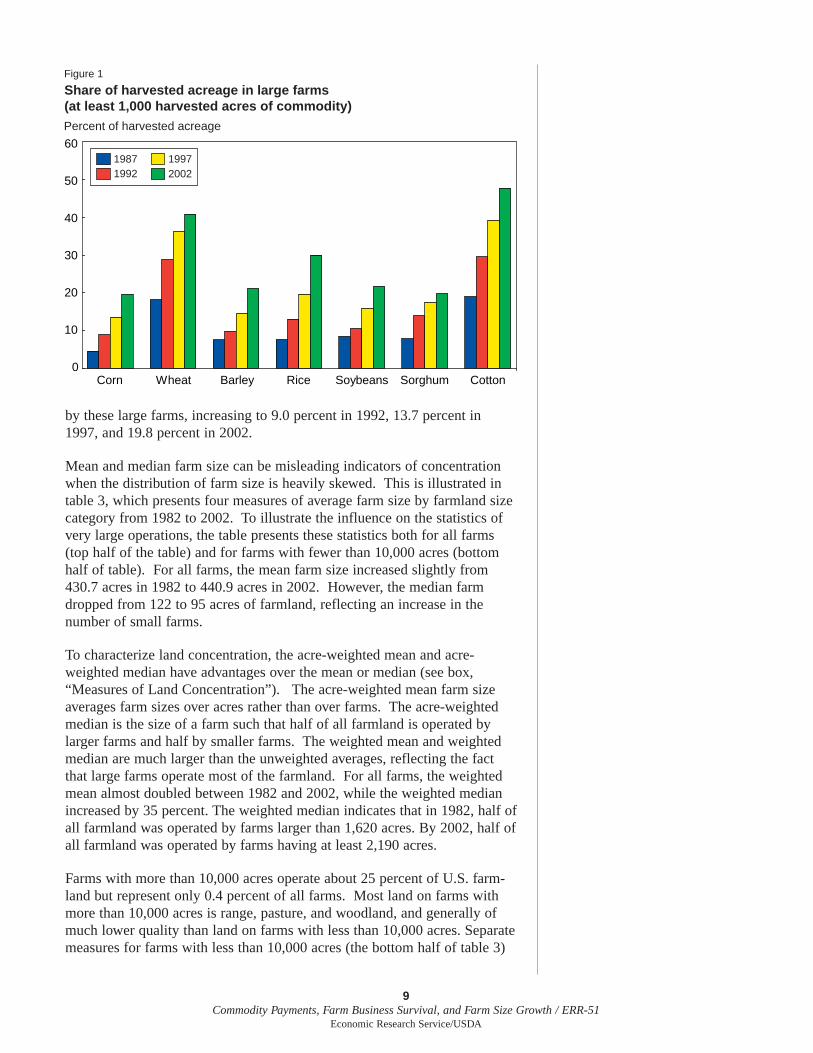
by these large farms, increasing to 9.0 percent in 1992, 13.7 percent in1997, and 19.8 percent in 2002.
Mean and median farm size can be misleading indicators of concentrationwhen the distribution of farm size is heavily skewed. This is illustrated intable 3, which presents four measures of average farm size by farmland sizecategory from 1982 to 2002. To illustrate the influence on the statistics ofvery large operations, the table presents these statistics both for all farms(top half of the table) and for farms with fewer than 10,000 acres (bottomhalf of table). For all farms, the mean farm size increased slightly from430.7 acres in 1982 to 440.9 acres in 2002. However, the median farmdropped from 122 to 95 acres of farmland, reflecting an increase in thenumber of small farms.
To characterize land concentration, the acre-weighted mean and acre-weighted median have advantages over the mean or median (see box,“Measures of Land Concentration”). The acre-weighted mean farm sizeaverages farm sizes over acres rather than over farms. The acre-weightedmedian is the size of a farm such that half of all farmland is operated bylarger farms and half by smaller farms. The weighted mean and weightedmedian are much larger than the unweighted averages, reflecting the factthat large farms operate most of the farmland. For all farms, the weightedmean almost doubled between 1982 and 2002, while the weighted medianincreased by 35 percent. The weighted median indicates that in 1982, half ofall farmland was operated by farms larger than 1,620 acres. By 2002, half ofall farmland was operated by farms having at least 2,190 acres.
Farms with more than 10,000 acres operate about 25 percent of U.S. farm-land but represent only 0.4 percent of all farms. Most land on farms withmore than 10,000 acres is range, pasture, and woodland, and generally ofmuch lower quality than land on farms with less than 10,000 acres. Separatemeasures for farms with less than 10,000 acres (the bottom half of table 3)
9Commodity Payments, Farm Business Survival, and Farm Size Growth / ERR-51
Economic Research Service/USDA
Figure 1
Share of harvested acreage in large farms(at least 1,000 harvested acres of commodity)Percent of harvested acreage
0
10
20
30
40
50
60
Corn Wheat Barley Rice Soybeans Sorghum Cotton
199720021992
1987
10Commodity Payments, Farm Business Survival, and Farm Size Growth / ERR-51
Economic Research Service/USDA
Measures of Land Concentration
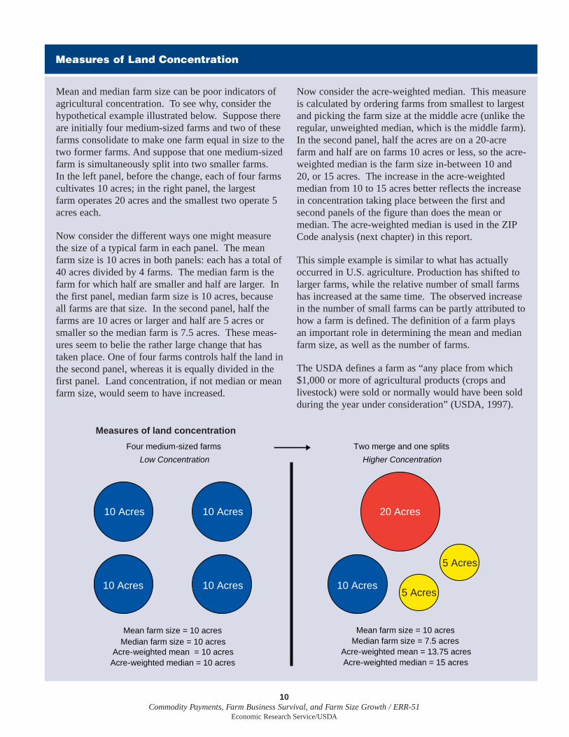
Mean and median farm size can be poor indicators ofagricultural concentration. To see why, consider thehypothetical example illustrated below. Suppose thereare initially four medium-sized farms and two of thesefarms consolidate to make one farm equal in size to thetwo former farms. And suppose that one medium-sizedfarm is simultaneously split into two smaller farms.In the left panel, before the change, each of four farmscultivates 10 acres; in the right panel, the largest farm operates 20 acres and the smallest two operate 5acres each.
Now consider the different ways one might measurethe size of a typical farm in each panel. The meanfarm size is 10 acres in both panels: each has a total of40 acres divided by 4 farms. The median farm is thefarm for which half are smaller and half are larger. Inthe first panel, median farm size is 10 acres, becauseall farms are that size. In the second panel, half thefarms are 10 acres or larger and half are 5 acres orsmaller so the median farm is 7.5 acres. These meas-ures seem to belie the rather large change that hastaken place. One of four farms controls half the land inthe second panel, whereas it is equally divided in thefirst panel. Land concentration, if not median or meanfarm size, would seem to have increased.
Now consider the acre-weighted median. This measureis calculated by ordering farms from smallest to largestand picking the farm size at the middle acre (unlike theregular, unweighted median, which is the middle farm).In the second panel, half the acres are on a 20-acrefarm and half are on farms 10 acres or less, so the acre-weighted median is the farm size in-between 10 and20, or 15 acres. The increase in the acre-weightedmedian from 10 to 15 acres better reflects the increasein concentration taking place between the first andsecond panels of the figure than does the mean ormedian. The acre-weighted median is used in the ZIPCode analysis (next chapter) in this report.
This simple example is similar to what has actuallyoccurred in U.S. agriculture. Production has shifted tolarger farms, while the relative number of small farmshas increased at the same time. The observed increasein the number of small farms can be partly attributed tohow a farm is defined. The definition of a farm playsan important role in determining the mean and medianfarm size, as well as the number of farms.
The USDA defines a farm as “any place from which$1,000 or more of agricultural products (crops andlivestock) were sold or normally would have been soldduring the year under consideration” (USDA, 1997).
Two merge and one splits
Measures of land concentration
Four medium-sized farms
Higher ConcentrationLow Concentration
Median farm size = 10 acresweighted mean = 10 acres
Mean farm size = 10 acres
Acre-Acre-weighted median = 10 acres
Mean farm size = 10 acresMedian farm size = 7.5 acres
Acre-weighted mean = 13.75 acresAcre-weighted median = 15 acres
10 Acres
10 Acres
20 Acres10 Acres
10 Acres10 Acres
5 Acres
5 Acres
11Commodity Payments, Farm Business Survival, and Farm Size Growth / ERR-51
Economic Research Service/USDA
This definition includes many small operations forwhich farming contributes only a small share of farmhousehold income. The $1,000 figure has remainedunchanged since the 1974 census, so inflation haseffectively increased the number of small operationsthat qualify as farms. Other changes in the definitionmay have also increased the count of small farms.1
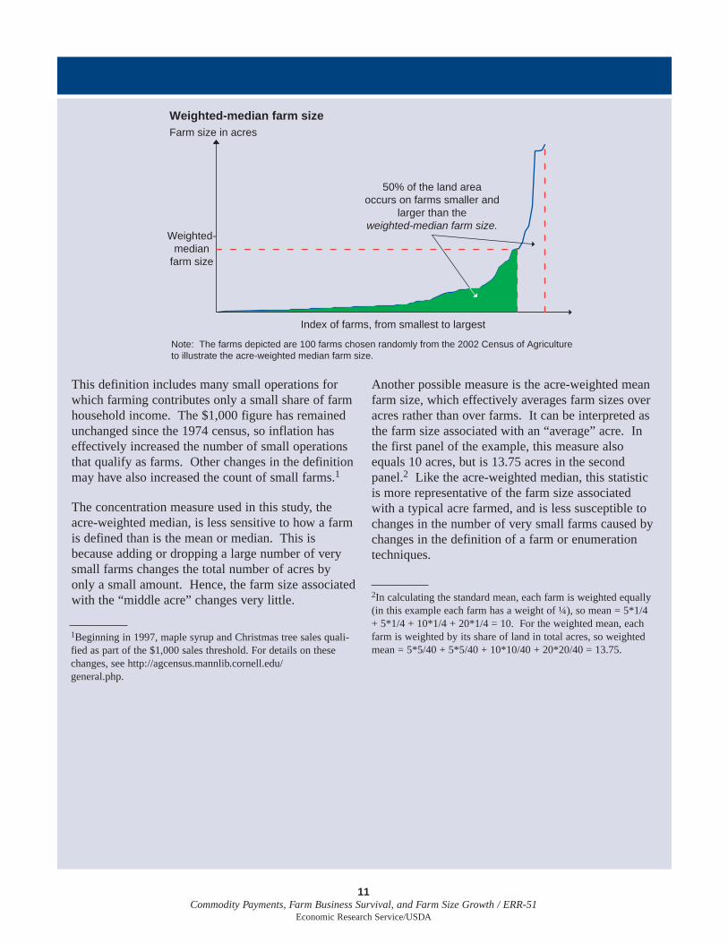
The concentration measure used in this study, theacre-weighted median, is less sensitive to how a farmis defined than is the mean or median. This isbecause adding or dropping a large number of verysmall farms changes the total number of acres byonly a small amount. Hence, the farm size associatedwith the “middle acre” changes very little.
Another possible measure is the acre-weighted meanfarm size, which effectively averages farm sizes overacres rather than over farms. It can be interpreted asthe farm size associated with an “average” acre. Inthe first panel of the example, this measure alsoequals 10 acres, but is 13.75 acres in the secondpanel.2 Like the acre-weighted median, this statisticis more representative of the farm size associatedwith a typical acre farmed, and is less susceptible tochanges in the number of very small farms caused bychanges in the definition of a farm or enumerationtechniques.
Weighted-median farm sizeFarm size in acres
Weighted-median
farm size
50% of the land areaoccurs on farms smaller and
larger than theweighted-median farm size.
Index of farms, from smallest to largest
Note: The farms depicted are 100 farms chosen randomly from the 2002 Census of Agricultureto illustrate the acre-weighted median farm size.
2In calculating the standard mean, each farm is weighted equally(in this example each farm has a weight of ¼), so mean = 5*1/4+ 5*1/4 + 10*1/4 + 20*1/4 = 10. For the weighted mean, eachfarm is weighted by its share of land in total acres, so weightedmean = 5*5/40 + 5*5/40 + 10*10/40 + 20*20/40 = 13.75.
1Beginning in 1997, maple syrup and Christmas tree sales quali-fied as part of the $1,000 sales threshold. For details on thesechanges, see http://agcensus.mannlib.cornell.edu/general.php.

show similar patterns for the mean, median, and weighted-median measures,but the weighted mean, which is more sensitive to outliers, differs from thetrend for all farms. For farms with less than 10,000 acres, the weightedmean increased by 20.7 percent between 1982 and 2002.
How Have Commodity Program PaymentsChanged Over Time?
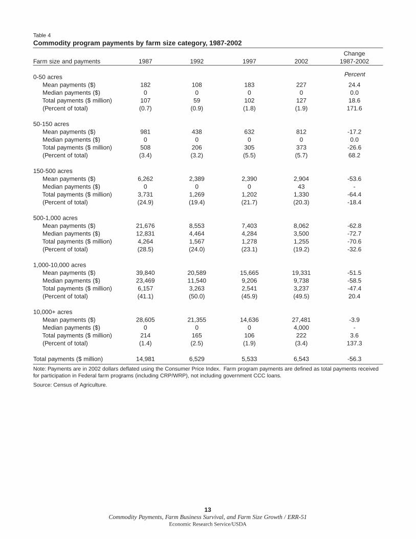
Commodity program payments (see box, “Defining Commodity ProgramPayments”) per farm are closely associated with farm size in all censusyears from 1987 to 2002. Mean program payments per farm increase withfarm size class up to 10,000 acres of farmland (table 4). In 2002, themedian payment for farms operating 1,000-10,000 acres was $9,738—almost three times the median payment for farms operating 500-1,000 acres,and about 200 times the median payment for farms with 150 to 500 acres offarmland. For some census years, very large farms operating more than10,000 acres actually received lower program payments per farm than farmsoperating 1,000-10,000 acres. A smaller portion of land managed by thesevery large farms is cultivated with crops normally targeted by commodityprograms. Farmland as defined by the census includes pasture, range,woodland, and other land, some of which is not actively used in farmproduction activities.
Large farms receive an increasingly large share of program payments. Theshare of payments going to farms with 1,000-10,000 acres increased from41.1 percent of all payments in 1987 to 49.5 percent in 2002. During thesame period, farms with 150-1,000 acres received a smaller share of totalpayments, while farms with fewer than 150 acres received an increasingshare (from 4.1 percent to 7.6 percent in 2002), reflecting their growingnumbers. Still, over half of all farms with less than 150 acres receive nocommodity program payments—a fact that has not changed since 1987.The share of payments going to farms operating more than 10,000 acresalso increased over time (table 4).
12Commodity Payments, Farm Business Survival, and Farm Size Growth / ERR-51
Economic Research Service/USDA
13Commodity Payments, Farm Business Survival, and Farm Size Growth / ERR-51
Economic Research Service/USDA
Table 4
Commodity program payments by farm size category, 1987-2002
ChangeFarm size and payments 1987 1992 1997 2002 1987-2002
0-50 acres Percent
Mean payments ($) 182 108 183 227 24.4Median payments ($) 0 0 0 0 0.0Total payments ($ million) 107 59 102 127 18.6(Percent of total) (0.7) (0.9) (1.8) (1.9) 171.6
50-150 acresMean payments ($) 981 438 632 812 -17.2Median payments ($) 0 0 0 0 0.0Total payments ($ million) 508 206 305 373 -26.6(Percent of total) (3.4) (3.2) (5.5) (5.7) 68.2
150-500 acresMean payments ($) 6,262 2,389 2,390 2,904 -53.6Median payments ($) 0 0 0 43 -Total payments ($ million) 3,731 1,269 1,202 1,330 -64.4(Percent of total) (24.9) (19.4) (21.7) (20.3) -18.4
500-1,000 acresMean payments ($) 21,676 8,553 7,403 8,062 -62.8Median payments ($) 12,831 4,464 4,284 3,500 -72.7Total payments ($ million) 4,264 1,567 1,278 1,255 -70.6(Percent of total) (28.5) (24.0) (23.1) (19.2) -32.6
1,000-10,000 acresMean payments ($) 39,840 20,589 15,665 19,331 -51.5Median payments ($) 23,469 11,540 9,206 9,738 -58.5Total payments ($ million) 6,157 3,263 2,541 3,237 -47.4(Percent of total) (41.1) (50.0) (45.9) (49.5) 20.4
10,000+ acresMean payments ($) 28,605 21,355 14,636 27,481 -3.9Median payments ($) 0 0 0 4,000 -Total payments ($ million) 214 165 106 222 3.6(Percent of total) (1.4) (2.5) (1.9) (3.4) 137.3
Total payments ($ million) 14,981 6,529 5,533 6,543 -56.3
Note: Payments are in 2002 dollars deflated using the Consumer Price Index. Farm program payments are defined as total payments receivedfor participation in Federal farm programs (including CRP/WRP), not including government CCC loans.
Source: Census of Agriculture.

14Commodity Payments, Farm Business Survival, and Farm Size Growth / ERR-51
Economic Research Service/USDA
Defining Commodity Program Payments
Although the Federal Government has providedpayments to farmers since the Great Depression, theprograms that provide payments have changedmarkedly over time. In recent decades, mostpayments have been tied to a farm’s “base acres,” ameasure of historical plantings of program crops, andto historical program crop yields. Program yieldswere fixed in 1985 (at an average of 1981-85 yields)until 2002. Base acres were fixed under the 1996Farm Act (production flexibility contract acreage).Until 2002, program crops included barley, corn,cotton, oats, rice, sorghum, and wheat.
Payments tied to base acres have fluctuated over time,depending on whether and to what extent marketprices fell below program-set target prices. In 1987and 1992, participation in government programs alsorequired farms to idle a share of their base. In theseyears farmers may have chosen not to participate ingovernment programs in order to avoid annualacreage reduction requirements. By 1992, farmerscould plant nonbase or other base crops on their baseacres in accordance with flexibility rules, whichchanged over time. By 1997, annual acreage reduc-tion programs were eliminated and farmers weregiven almost complete flexibility in planting.
In addition to payments tied to base acres, farmershave also received loan deficiency payments from themarketing loan program. These payments depend oncurrent production, not base acres, and the paymentamount depends on the difference between marketprices and loan rates set by the program. Marketingloan payments were available for soybeans and minoroilseeds in addition to program crops that receivepayments tied to base acres. Some kinds ofmarketing loan benefits are not included in our databecause the census of agriculture does collect infor-mation about them.
The census of agriculture does not classify paymentsaccording to type beyond distinguishing paymentsfrom the Conservation Reserve Program (CRP) and
Wetland Reserve Program (WRP). This studyconsiders total payments net of CRP and WRPpayments because these program payments are gener-ally small and likely influence concentration growthdifferently than other kinds of payments. Data onpayments were available starting in 1987. For the1987, 1992, and 1997 censuses, respondents wereasked for (1) “the amount received from CCC loans”by crop, (2) “total amount received for participationin Federal farm programs (do not include CCCloans),” and (3) “of the total amount [in 2] how muchwas received for participation in the CRP and WRP?”For 1987, 1992, and 1997, the value from (2) minusthe value from (3) was used in the analysis, exceptfor table 4.
In 2002, respondents were asked for (1) “totalamount received in 2002 from Government CCCloans for all crops,” (2) “how much was received forparticipation in the Conservation Reserve Programand Wetlands Reserve Program (CRP and WRP)” and(3) “amount received from other participation in otherFederal farm programs (include loan deficiencypayments).” For 2002, the value in (3) would be theappropriate measure of payments, but 2002 paymentswere not used in the analysis linking payments toconcentration because we use past payments toobserve subsequent growth.
Total commodity program payments recorded by thecensus are substantially below the net outlays tofarmers reported by the USDA. For example, in 2002,census respondents reported commodity programpayments net of Commodity Credit Corporation(CCC) loans and CRP and WRP payments totaling$5.2 billion. In contrast, the Farm Service Agencybudget reports that total direct cash paymentsexcluding conservation payments totaled $9.7 billion(USDA/ERS, 2007). Part of this discrepancy couldbe explained by the fact that landlords received asubstantial portion of commodity program payments,and many landlords were not operators, so they werenot included in the census of agriculture.
Chapter 4
Commodity Program Payments and theConcentration of CroplandTo focus more clearly on the impact of payments on crop producers, crop-land (versus farmland) is used to characterize land concentration at the local(ZIP Code) level. Weighted-median cropland is constructed in the same wayas weighted-median farmland in the previous chapter (cropland excludespasture, range, woodland, and other minor uses).8 The analysis includesalmost all farms and ZIP Codes in the census of agriculture.
First, the study compares percentage changes in cropland concentrationbetween consecutive census periods of ZIP Codes having different levels ofpayments. This indicates whether concentration increased more in regionshaving higher average payments per acre than in regions with lower averagepayments. Even if programs target farms that happen to be larger due to thenature of the crops they grow (that is, some crops are land-intensive), thereis no apparent reason to expect programs to target farm types more inclinedto grow in size over time. And, by examining percentage changes, growth isscaled relative to initial concentration levels.
Although a comparison of changes can control for many factors, theapproach is not infallible. It might be that corn, wheat, cotton, and othercrop farms traditionally targeted by programs have grown more concen-trated for reasons other than government programs. To address this concern,the study controls for initial farm size and for ZIP Code location. Thisapproach restricts comparisons to those between ZIP Codes with similarinitial farm sizes that are close to each other geographically, and thus likelyto have similar climate, soils, and crop types.
It is possible that areas with high yields, and hence higher payments, also havebetter land quality (flatter, more fertile soil, etc.). If scale-enhancing technolog-ical change favored higher quality land over lower quality land for the samecrop, this could explain a correlation between payments and subsequent growthin land concentration. To account for variation in land quality, the studycontrols for initial crop sales per acre and the share of all land in crops.
If it were participation in farm commodity programs and not the paymentlevels associated with participation that drove farm size changes, one mightexpect a similar change in farm size between crops with higher and lowerpayment levels. For example, payments (per acre) tied to cotton productiontend to be higher than those tied to corn, while corn payments tend to behigher than for wheat. Examining farm growth rates over a range ofpayment levels demonstrates that concentration growth steadily increaseswith steadily increasing payment levels.
Of course, other factors cause payment levels to differ across ZIP Codes(see box, “Defining Commodity Program Payments”). One source of varia-tion in payment levels stems from regional differences in crop mix. Ofparticular importance is farmers’ planting decisions and yield outcomes.Yields between 1981 and 1985 determined 1985 base acres and programcrop yields. Particularly high or low yields in those years because ofweather variation would have longrun consequences in terms of payment
8An analysis using farmland instead ofcropland produced qualitatively simi-lar results.
15Commodity Payments, Farm Business Survival, and Farm Size Growth / ERR-32
Economic Research Service/USDA
16Commodity Payments, Farm Business Survival, and Farm Size Growth / ERR-51
Economic Research Service/USDA
Zip Code Data
The data used for this analysis include all ZIP Codesrecorded in the census of agriculture that had at leastthree farms in each of the four census years examined(1987, 1992, 1997, and 2002). The analysis begins in1987, the first year for which farm-specific data oncommodity program payments are available. Thestudy examines ZIP Code areas because they are thesmallest geographic unit where farms can be locatedwith the data. This provides more observations andmore variability in the concentration and paymentmeasures than a county-level analysis would. Localvariation in payment levels and concentration growthis important when attempting to identify the effect ofpayments on concentration while controlling forfactors that vary geographically.
ZIP Code areas, like counties, vary markedly in size,with rural ZIP Codes generally larger than urban ZIPCodes and Western ZIP Codes generally larger thanthose farther east. To account for this variation, thestudy examines payments per acre of cropland ratherthan total payments. This standardization makes thepayments measure insensitive to the size of ZIP Codeareas. The concentration measure is not sensitive tothe land area of the ZIP Code and therefore does notrequire standardization.
ZIP Codes can change over time. Most changes haveoccurred in more urban areas undergoing rapid popu-lation growth and where agriculture is less prevalent,which mitigates the issue for this analysis. When ZIPCodes do change, it is usually because one ZIP Codeis split into two or more ZIP Codes, with one arearetaining the old ZIP Code and the other(s) assigned anew code. Sometimes individual ZIP Codes areassigned to universities or large companies, and thiscan also change over time. Because the studyrestricts the analysis to ZIP Codes appearing in allfour censuses, all farms in areas with new ZIP Codesare omitted. However, there are a few ZIP Codes thatdecreased in size between 1987 and 2002, with partof the earlier ZIP Code area split off into new ZIPCodes that were dropped. These changes, however,would not be expected to be systematically related topayments per acre or concentration measures.
Another consideration is that many farms likelystraddle ZIP Codes. This issue is not likely to causesignificant bias in this analysis because the ZIP Codeassociated with any particular farm is unlikely tochange from one census to the next. Measurementissues may arise when farms with different ZIPCodes consolidate, causing reassignment of land fromone ZIP Code to another. Such changes may createmore variability in the concentration measure overtime for ZIP Codes affected by consolidation, butthere is no reason to expect this variability to be asso-ciated with commodity program payments per acre orother determinants of farm size.1
The census of agriculture reported farms in 32,959ZIP Codes in 1987, 34,202 in 1992, 34,408 in 1997,and 33,548 in 2002; 23,293 ZIP Codes had 3 or morefarms reporting in all censuses.2 Of these 23,293 ZIPCodes, observations with undefined variables orextreme outliers are dropped, resulting in 21,524 ZIPCodes. Although the sample drops about a third ofall U.S. ZIP Codes containing farms, it drops a muchsmaller share of total farms. The sample includes1,716,814; 1,524,783; 1,541,547; and 1,341,306farms in the 4 census years, compared with1,799,926; 1,621,263; 1,653,098; and 1,486,895farms in the raw census files.3
1 Only a small portion of farms are dropped from the analysisbecause their ZIP codes were dropped. This suggests most farmsare in areas relatively unaffected by changes in ZIP Codes. Andthe farms dropped are predominantly very small farms, whichhave little influence on the weighted-median farm size.
2 These counts compare to a nationwide total of about 43,000ZIP Codes currently in the United States.
3 These numbers refer to actual census observations. Publishedcensus estimates of farm numbers are higher to account for non-response probabilities. Nonresponse weights were used in com-puting tables 2-4.

levels. Similarly, because base acres were fixed in 1996, cropping decisionsprior to 1996 affected payment levels for many years.
Another factor driving variation in payments is historical participation ingovernment farm programs. In the late 1980s, agricultural program restric-tions may have discouraged some farmers from participating. Participationrequired farmers to limit their plantings to a share of acres historicallyplanted and required that a certain portion be idled (called the AcreageReduction Program). Farmers with environmentally fragile land (e.g.,highly erodible) were also required to follow certain practices to limit envi-ronmental damages stemming from the cropping activities.9 These costlyparticipation restrictions probably limited program participation.10
For each ZIP Code region, the study estimates concentration using the acre-weighted median cropland area. This measure is the farm size at which halfthe cropland in the ZIP Code is operated by farms with more cropland andhalf the cropland is operated by farms with less cropland.
Figure 4 illustrates how the distribution of farm sizes has changed since1987. The figure shows the frequency distributions of cropland concentra-tion in the census years from 1987 to 2002. The horizontal axis is concen-tration, plotted on a logarithmic scale, and the vertical axis measures thefrequency of ZIP Codes at each concentration level. The area under eachcurve equals one, by definition, so the area beneath the curve between anytwo points represents the share of ZIP Codes that are in the size range. Thehorizontal axis is plotted on a logarithmic scale where each step represents aten-fold increase in farm size (rather than an increase of 10 units). Becausethere are relatively few ZIP Code areas with very high levels of concentra-tion (the distribution is highly skewed), the logarithmic scale allows for aclearer representation of the whole distribution and more clearly illustrates
17Commodity Payments, Farm Business Survival, and Farm Size Growth / ERR-51
Economic Research Service/USDA
Figure 4Distribution of cropland concentration across ZIP Codes, 1987-2002
Density of ZIP Code areas
Acre-weighted median (acres)
Note: Data are from census of agriculture 1987, 1992, 1997, and 2002. Sample includes allZIP Codes with at least three farm operations reporting in each year.
1987199219972002
0.4
0.3
0.2
0.1
01 01 100 1,000 10,000
10 Prior to 1996, between 15 and 40percent of eligible cropland was notenrolled in a Federal program (USDA,various years).
9 See Claasen et al. for a description ofcross-compliance provisions.
the continuous temporal shift. The figure shows cropland distributionsshifting markedly to the right: the share of ZIP Codes with weighted-medianfarm size above 600 acres increased every census from 1987 to 2002, indi-cating a relative increase in cropland controlled by larger farms.
Descriptive Statistics for ZIP Codes
The empirical approach is to compare how cropland concentration changesfor ZIP Codes with different initial commodity program payments per acre(total commodity program payments divided by total cropland). The studymeasures changes in concentration over the three 5-year periods betweencensuses (1987-92, 1992-97, and 1997-2002). For example, it measureshow payments per acre in 1987 correlate with changes in concentrationfrom 1987 to 1992. It also measures the longrun relationship betweenpayments per acre in 1987 and total percentage growth in concentrationfrom 1987 to 2002.
For 1987, 1992, and 1997, ZIP Codes are sorted into six groups: the firstgroup includes those ZIP Codes with zero program payments; the remainingZIP Codes are sorted into five quintiles according to their level of paymentsper acre, with each quintile having the same number of ZIP Codes. Thereare two advantages to examining payment quintiles rather than estimating alinear or continuous relationship between payments per acre and concentra-tion growth. First, estimating separate concentration measures for eachquintile allows for the identification of nonlinear relationships betweenpayment levels and concentration, if they exist. Second, pooling manyobservations into discrete categories of equal size greatly reduces the influ-ence of miscoded or anomalous data.
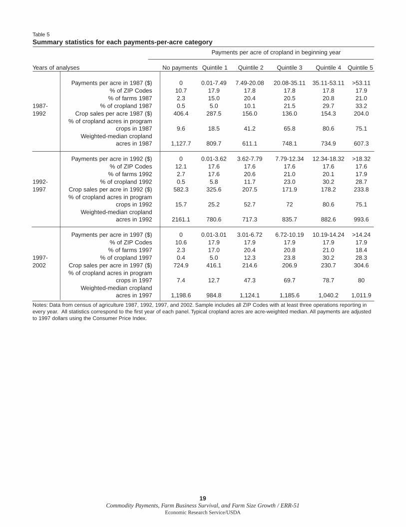
For each of the six payment groups, table 5 reports summary statistics forthe proportion of ZIP Codes, farms, and cropland; crop sales per acre; shareof cropland in program crops and soybeans (a common rotation crop); andcropland concentration (weighted-median cropland), all for the beginningyear of each census panel. The payment levels that divide quintiles change from one census year to the next as the general level of paymentsvaries, mainly due to changing commodity prices and target prices set byfarm policy.
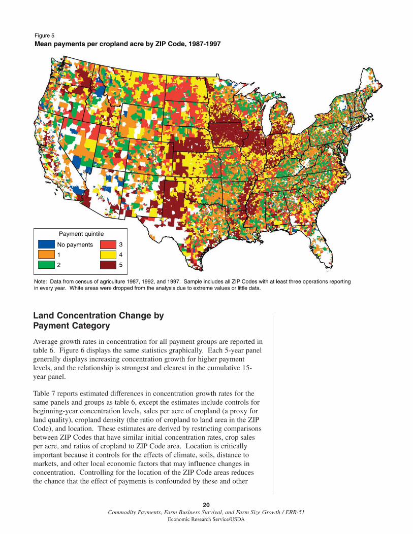
As one would expect, the share of cropland in program crops increases withpayment levels. With the exception of the no-payment group, typical farmsize (initial concentration) is not markedly different between the paymentgroups in the initial year, but grows more for the higher payment groups inthe more recent panels. Figure 5 maps ZIP Codes according to the croplandpayment groups used for the longrun analysis.
18Commodity Payments, Farm Business Survival, and Farm Size Growth / ERR-51
Economic Research Service/USDA
19Commodity Payments, Farm Business Survival, and Farm Size Growth / ERR-51
Economic Research Service/USDA
Table 5
Summary statistics for each payments-per-acre category
Payments per acre of cropland in beginning year
Years of analyses No payments Quintile 1 Quintile 2 Quintile 3 Quintile 4 Quintile 5
Payments per acre in 1987 ($) 0 0.01-7.49 7.49-20.08 20.08-35.11 35.11-53.11 >53.11% of ZIP Codes 10.7 17.9 17.8 17.8 17.8 17.9% of farms 1987 2.3 15.0 20.4 20.5 20.8 21.0
1987- % of cropland 1987 0.5 5.0 10.1 21.5 29.7 33.21992 Crop sales per acre 1987 ($) 406.4 287.5 156.0 136.0 154.3 204.0
% of cropland acres in programcrops in 1987 9.6 18.5 41.2 65.8 80.6 75.1
Weighted-median croplandacres in 1987 1,127.7 809.7 611.1 748.1 734.9 607.3
Payments per acre in 1992 ($) 0 0.01-3.62 3.62-7.79 7.79-12.34 12.34-18.32 >18.32% of ZIP Codes 12.1 17.6 17.6 17.6 17.6 17.6% of farms 1992 2.7 17.6 20.6 21.0 20.1 17.9
1992- % of cropland 1992 0.5 5.8 11.7 23.0 30.2 28.71997 Crop sales per acre in 1992 ($) 582.3 325.6 207.5 171.9 178.2 233.8
% of cropland acres in programcrops in 1992 15.7 25.2 52.7 72 80.6 75.1
Weighted-median croplandacres in 1992 2161.1 780.6 717.3 835.7 882.6 993.6
Payments per acre in 1997 ($) 0 0.01-3.01 3.01-6.72 6.72-10.19 10.19-14.24 >14.24% of ZIP Codes 10.6 17.9 17.9 17.9 17.9 17.9% of farms 1997 2.3 17.0 20.4 20.8 21.0 18.4
1997- % of cropland 1997 0.4 5.0 12.3 23.8 30.2 28.32002 Crop sales per acre in 1997 ($) 724.9 416.1 214.6 206.9 230.7 304.6
% of cropland acres in programcrops in 1997 7.4 12.7 47.3 69.7 78.7 80
Weighted-median croplandacres in 1997 1,198.6 984.8 1,124.1 1,185.6 1,040.2 1,011.9
Notes: Data from census of agriculture 1987, 1992, 1997, and 2002. Sample includes all ZIP Codes with at least three operations reporting inevery year. All statistics correspond to the first year of each panel. Typical cropland acres are acre-weighted median. All payments are adjustedto 1997 dollars using the Consumer Price Index.
Land Concentration Change by Payment Category
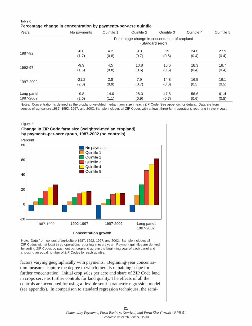
Average growth rates in concentration for all payment groups are reported intable 6. Figure 6 displays the same statistics graphically. Each 5-year panelgenerally displays increasing concentration growth for higher paymentlevels, and the relationship is strongest and clearest in the cumulative 15-year panel.
Table 7 reports estimated differences in concentration growth rates for thesame panels and groups as table 6, except the estimates include controls forbeginning-year concentration levels, sales per acre of cropland (a proxy forland quality), cropland density (the ratio of cropland to land area in the ZIPCode), and location. These estimates are derived by restricting comparisonsbetween ZIP Codes that have similar initial concentration rates, crop salesper acre, and ratios of cropland to ZIP Code area. Location is criticallyimportant because it controls for the effects of climate, soils, distance tomarkets, and other local economic factors that may influence changes inconcentration. Controlling for the location of the ZIP Code areas reducesthe chance that the effect of payments is confounded by these and other
20Commodity Payments, Farm Business Survival, and Farm Size Growth / ERR-51
Economic Research Service/USDA
Figure 5
No payments
1
2
3
4
5
Payment quintile
Mean payments per cropland acre by ZIP Code, 1987-1997
Note: Data from census of agriculture 1987, 1992, and 1997. Sample includes all ZIP Codes with at least three operations reportingin every year. White areas were dropped from the analysis due to extreme values or little data.
factors varying geographically with payments. Beginning-year concentra-tion measures capture the degree to which there is remaining scope forfurther concentration. Initial crop sales per acre and share of ZIP Code landin crops serve as further controls for land quality. The effects of all thecontrols are accounted for using a flexible semi-parametric regression model(see appendix). In comparison to standard regression techniques, the semi-
21Commodity Payments, Farm Business Survival, and Farm Size Growth / ERR-51
Economic Research Service/USDA
Table 6
Percentage change in concentration by payments-per-acre quintile
Years No payments Quintile 1 Quintile 2 Quintile 3 Quintile 4 Quintile 5
Percentage change in concentration of cropland (Standard error)
-8.8 4.2 9.3 19 24.8 27.9(1.7) (0.8) (0.7) (0.5) (0.4) (0.4)
-9.9 4.5 10.8 15.6 18.3 18.7(1.5) (0.8) (0.6) (0.5) (0.4) (0.4)
-21.2 2.8 7.9 14.8 16.5 16.1(2.0) (0.9) (0.7) (0.6) (0.5) (0.5)
-9.8 14.0 28.0 47.8 56.6 61.4(2.0) (1.1) (0.9) (0.7) (0.6) (0.5)
Notes: Concentration is defined as the cropland-weighted median farm size in each ZIP Code. See appendix for details. Data are from census of agriculture 1987, 1992, 1997, and 2002. Sample includes all ZIP Codes with at least three farm operations reporting in every year.
1987-92
1992-97
1997-2002
Long panel1987-2002
Figure 6
Change in ZIP Code farm size (weighted-median cropland)by payments-per-acre group, 1987-2002 (no controls)Percent
Concentration growth
1987-1992 1992-1997 1997-2002 Long panel:1987-2002
Note: Data from census of agriculture 1987, 1992, 1997, and 2002. Sample includes allZIP Codes with at least three operations reporting in every year. Payment quintiles are derivedby sorting ZIP Codes by payment per cropland acre in the beginning year of each panel andchoosing an equal number of ZIP Codes for each quintile.
80
60
40
20
0
-20
No paymentsQuintile 1 Quintile 2 Quintile 3 Quintile 4 Quintile 5
parametric model requires fewer assumptions about the way these controlvariables influence concentration growth.
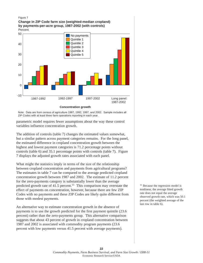
The addition of controls (table 7) changes the estimated values somewhat,but a similar pattern across payment categories remains. For the long panel,the estimated difference in cropland concentration growth between thehighest and lowest payment categories is 71.2 percentage points withoutcontrols (table 6) and 35.1 percentage points with controls (table 7). Figure7 displays the adjusted growth rates associated with each panel.
What might the statistics imply in terms of the size of the relationshipbetween cropland concentration and payments from agricultural programs?The estimates in table 7 can be compared to the average predicted croplandconcentration growth between 1987 and 2002. The estimate of 11.2 percentfor the zero-payments category is substantially lower than the averagepredicted growth rate of 41.5 percent.11 This comparison may overstate theeffect of payments on concentration, however, because there are few ZIPCodes with no payments and these ZIP Codes are likely quite different fromthose with modest payments.
An alternative way to estimate concentration growth in the absence ofpayments is to use the growth predicted for the first payment quintile (23.6percent) rather than the zero-payments group. This alternative comparisonsuggests that about 43 percent of growth in cropland concentration between1987 and 2002 is associated with commodity program payments (23.6percent with low payments versus 41.5 percent with average payments).
22Commodity Payments, Farm Business Survival, and Farm Size Growth / ERR-51
Economic Research Service/USDA
11 Because the regression model isnonlinear, the average fitted growthrate does not equal the averageobserved growth rate, which was 50.1percent (the weighted average of thelast row in table 6).
Figure 7
Change in ZIP Code farm size (weighted-median cropland)by payments-per-acre group, 1987-2002 (with controls)Percent
Concentration growth
1987-1992 1992-1997 1997-2002 Long panel:1987-2002
No paymentsQuintile 1 Quintile 2 Quintile 3 Quintile 4 Quintile 5
Note: Data are from census of agriculture 1987, 1992, 1997, and 2002. Sample includes allZIP Codes with at least three farm operations reporting in each year.
50
40
30
20
10
0
-10

23Commodity Payments, Farm Business Survival, and Farm Size Growth / ERR-51
Economic Research Service/USDA
Table 7
Percentage change in ZIP Code farm size (weighted-median cropland) by payments-per-acre quintitle group, with controls
Years No payments Quintile 1 Quintile 2 Quintile 3 Quintile 4 Quintile 5
Percentage change in concentration of cropland (Standard error)
-4.3 2.9 9.8 15.7 21.4 22.1(1.7) (1.8) (1.8) (1.8) (1.8) (1.8)
-5.3 3.3 7.5 12.3 14.7 15.2(1.7) (1.8) (1.8) (1.8) (1.8) (1.8)
-11.4 -0.7 4.3 10.1 13.4 7.1(1.7) (1.8) (1.8) (1.8) (1.8) (1.8)
11.2 23.6 29.9 39.7 46.3 46.3(1.8) (2.0) (2.0) (2.3) (2.3) (2.4)
Notes: This table reports estimated effects of the payment quintiles on concentration growth after controlling for location and concentration, salesper acre of cropland, and the ratio of cropland to area in each ZIP Code in the beginning year of each panel. Effects were estimated using asemi-parametric generalized additive regression model. Concentration is defined as the weighted-median farm size in each ZIP Code. For thelong panel, quintiles are calculated using payments per acre in 1987. An appendix provides more detail about the methods used. Data are fromcensus of agriculture 1987, 1992, 1997, and 2002. Sample includes all ZIP Codes with at least three farm operations reporting in every year.Extreme outliers were dropped from the analysis, as described in the appendix.
1987-92
1992-97
1997-2002
Long panel1987-2002
Chapter 5
Effect of Payments on Growth and Survival of FarmsThe change in concentration from one period to the next depends on the sizeof farms that survive, how much they grow if they survive, and the size ofnewly entering farms. Thus, to better understand how payments might beleading to higher concentration levels, it is useful to examine the relation-ship between payment levels and the survival and growth of individual farmbusinesses over time. These farm-level analyses complement the ZIP Code-level analysis and further indicate how payments could have altered farmstructure. The farm-level analyses consider only producers who specializedin program crops.12 This focus facilitates comparisons between farms withsimilar attributes. The study begins with an examination of farm survival,followed by an analysis of farm growth.
Payments and Farm Survival
For the survival analysis, the study compares the mean lifespans of farmsthat received different levels of commodity program payments. The studythen estimates how a farm’s probability of surviving changes over itslifespan, and compares this relationship for farms with high and low levelsof payments (see box, “Measuring the Duration of Farm BusinessSurvival”). Finally, the study estimates the effect of program payments onthe rate of farm business exit, and uses these estimates to simulate the effectof a policy that reduces payments by 50 percent for each farm.
The census of agriculture illustrates how survival rates change with the ageof the operation for farms with different commodity specializations (SICcodes). Table 8 presents the survival rates by SIC code for program cropfarms that were first observed in the 1982 census (these farms might haveinitiated production between 1979 and 1982, as 1978 was the year of theprevious census). About 50 percent of new farms exited within the first 5years. After 10 years, about 32 percent of the new farms remained in busi-ness, and after 15 years, 22.5 percent remained in business. These survivalrates are comparable to what has been reported for non-agricultural firms(e.g., Audretsch, 1991; Mata et al., 1995; Disney et al., 2003). Findings arealso consistent with earlier studies showing the probability of survivalgenerally increases with the age of the firm (Evans, 1987a; Evans, 1987b;Audretsch, 1991), as well as a recent ERS report that shows the larger afarm and the more experienced its operator, the less likely the farm is to exit(Hoppe and Korb, 2006).
Comparing Survival Rates of Farms WithDifferent Levels of Program Payments
To examine the relationship between program payments and farm businesssurvival, the study first compares the mean observed lifespan for farm busi-nesses of different sizes and different shares of payments in total sales.Total agricultural sales, like cropland or farmland area, is a measure of farm
24Commodity Payments, Farm Business Survival, and Farm Size Growth / ERR-51
Economic Research Service/USDA
12 The survival analyses focus on thosefarms specializing in wheat, rice, corn,soybeans, cash grains, or cotton. Thegrowth analyses exclude rice and cot-ton producers because there were toofew observations to perform crop-specific regressions. See Key andRoberts (2006) and Key and Roberts(2007) for more details.
25Commodity Payments, Farm Business Survival, and Farm Size Growth / ERR-51
Economic Research Service/USDA
Measuring the Duration of Farm Business Survival
Data used to estimate the relationship betweencommodity program payments and farm businesssurvival are from the census of agriculture conductedin 1987, 1992, and 1997 (individual records from the2002 census were not available at the time thisanalysis was performed). The census provides infor-mation about the duration of a farm business only if itwas continuously operated by the same individualand tracks operations over time using a Census FileNumber (CFN). The census defines a farm as out ofbusiness if there is no response to the census ques-tionnaire or if it is returned stating that the farm is nolonger operating. However, if a farm changes opera-tors through a business transaction or inheritance, theCFN may change even though the business is stilloperating. Hence, it is not possible to estimate theduration of a farm business based on how long theCFN appears in the census. Consequently, for theanalysis, a surviving farm is defined as one remainingin business and having the same operator; farmsremaining in business with a different operator wereremoved from the sample because it is not possible toobserve why an operation transferred ownership.1
This study examines the survival of farms that wereoperating in 1987—the first year the census of agri-culture began collecting information on commodityprogram payments. To increase sample homogeneity,the study focuses only on farms with Standard Indus-trial Classification (SIC) codes indicating they wereprimarily producers of wheat, rice, corn, soybeans,cotton, or “cash grains.” The sample includes the200,187 farms that had at least 10 acres of land and$10,000 in sales in 1987 and for which information
on all variables was available.2 The census allowsone to identify whether a farm business ceased oper-ating between 1987 and 1992, or between 1992 and1997, or whether it was still operating in 1997. Inaddition, the census records the year in which thecurrent operator began managing the operation.Therefore, the observed lifespan of the farm businessis defined as 1987 minus the year the operator initi-ated farming on the operation plus 2.5, 7.5, or 10,depending on whether the operation ceased operatingby 1992, ceased operating by 1997, or remained inbusiness in 1997.
The data have two characteristics that must beaccounted for in the estimation of the duration offarm business survival. First, if a farm operationremained in business in 1997, it is not possible toobserve the lifespan of the business; only that thebusiness was operating as of 1997. Second, thesample does not include businesses that exited priorto 1987. For example, of all businesses initiated in1980, only those businesses in 1987 that survived atleast 7 years are observed. Farms that exited before1987 are not observed. The regression techniqueused accounts for these data issues.
The regression controls for many other factors thatmight be associated with farm survival, includingspecialization as indicated by the farm SIC code,operator age, the year the farm began operating, thefarm’s organizational structure, the State in which thefarm operates, and the farm’s debt-to-asset ratio.Controlling for the year a farm began operatingcaptures effects stemming from time-specific events,such as changes in farm policy and the farm crisis ofthe early 1980s. More details can be found in Keyand Roberts (2006).
2 Deleting farms with less than $10,000 in sales (which representabout a fifth of the observations) focuses the analysis on farmhouseholds where farm business income is a larger share of totalhousehold income and where commodity program payments arethus more likely to play an important role in the decision to con-tinue farming. Whether or not these small farms are included inthe analysis has little influence on the results.
1 A farm was considered to have the same operator if the age ofthe operator differed by 5 years between consecutive censuses.
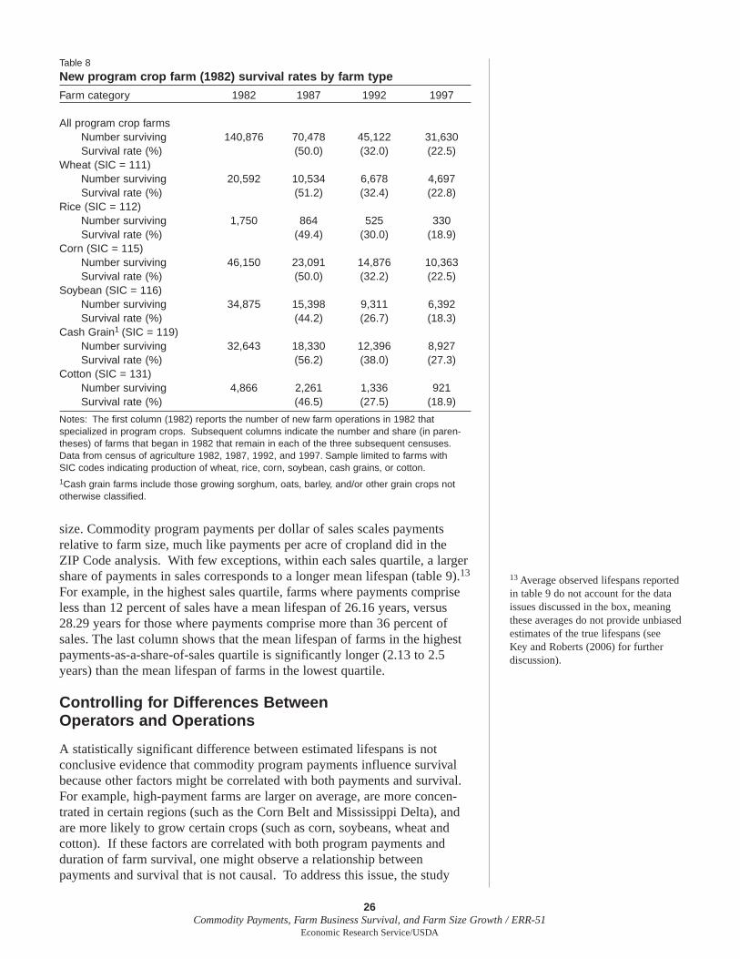
size. Commodity program payments per dollar of sales scales paymentsrelative to farm size, much like payments per acre of cropland did in the ZIP Code analysis. With few exceptions, within each sales quartile, a largershare of payments in sales corresponds to a longer mean lifespan (table 9).13
For example, in the highest sales quartile, farms where payments compriseless than 12 percent of sales have a mean lifespan of 26.16 years, versus28.29 years for those where payments comprise more than 36 percent ofsales. The last column shows that the mean lifespan of farms in the highestpayments-as-a-share-of-sales quartile is significantly longer (2.13 to 2.5years) than the mean lifespan of farms in the lowest quartile.
Controlling for Differences BetweenOperators and Operations
A statistically significant difference between estimated lifespans is notconclusive evidence that commodity program payments influence survivalbecause other factors might be correlated with both payments and survival.For example, high-payment farms are larger on average, are more concen-trated in certain regions (such as the Corn Belt and Mississippi Delta), andare more likely to grow certain crops (such as corn, soybeans, wheat andcotton). If these factors are correlated with both program payments andduration of farm survival, one might observe a relationship betweenpayments and survival that is not causal. To address this issue, the study
26Commodity Payments, Farm Business Survival, and Farm Size Growth / ERR-51
Economic Research Service/USDA
Table 8
New program crop farm (1982) survival rates by farm type
Farm category 1982 1987 1992 1997
All program crop farmsNumber surviving 140,876 70,478 45,122 31,630Survival rate (%) (50.0) (32.0) (22.5)
Wheat (SIC = 111)Number surviving 20,592 10,534 6,678 4,697Survival rate (%) (51.2) (32.4) (22.8)
Rice (SIC = 112)Number surviving 1,750 864 525 330Survival rate (%) (49.4) (30.0) (18.9)
Corn (SIC = 115)Number surviving 46,150 23,091 14,876 10,363Survival rate (%) (50.0) (32.2) (22.5)
Soybean (SIC = 116)Number surviving 34,875 15,398 9,311 6,392Survival rate (%) (44.2) (26.7) (18.3)
Cash Grain1 (SIC = 119)Number surviving 32,643 18,330 12,396 8,927Survival rate (%) (56.2) (38.0) (27.3)
Cotton (SIC = 131)Number surviving 4,866 2,261 1,336 921Survival rate (%) (46.5) (27.5) (18.9)
Notes: The first column (1982) reports the number of new farm operations in 1982 that specialized in program crops. Subsequent columns indicate the number and share (in paren-theses) of farms that began in 1982 that remain in each of the three subsequent censuses.Data from census of agriculture 1982, 1987, 1992, and 1997. Sample limited to farms with SIC codes indicating production of wheat, rice, corn, soybean, cash grains, or cotton.1Cash grain farms include those growing sorghum, oats, barley, and/or other grain crops nototherwise classified.
13 Average observed lifespans reportedin table 9 do not account for the dataissues discussed in the box, meaningthese averages do not provide unbiasedestimates of the true lifespans (seeKey and Roberts (2006) for furtherdiscussion).
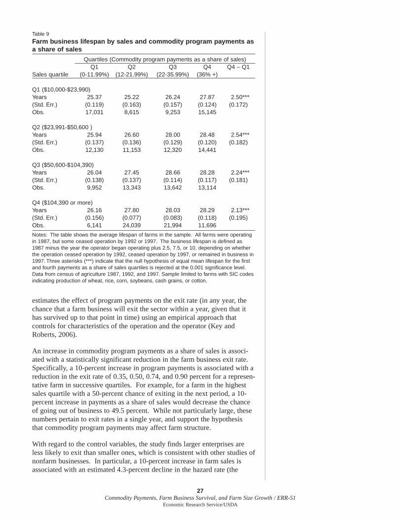
estimates the effect of program payments on the exit rate (in any year, thechance that a farm business will exit the sector within a year, given that ithas survived up to that point in time) using an empirical approach thatcontrols for characteristics of the operation and the operator (Key andRoberts, 2006).
An increase in commodity program payments as a share of sales is associ-ated with a statistically significant reduction in the farm business exit rate.Specifically, a 10-percent increase in program payments is associated with areduction in the exit rate of 0.35, 0.50, 0.74, and 0.90 percent for a represen-tative farm in successive quartiles. For example, for a farm in the highestsales quartile with a 50-percent chance of exiting in the next period, a 10-percent increase in payments as a share of sales would decrease the chanceof going out of business to 49.5 percent. While not particularly large, thesenumbers pertain to exit rates in a single year, and support the hypothesisthat commodity program payments may affect farm structure.
With regard to the control variables, the study finds larger enterprises areless likely to exit than smaller ones, which is consistent with other studies ofnonfarm businesses. In particular, a 10-percent increase in farm sales isassociated with an estimated 4.3-percent decline in the hazard rate (the
27Commodity Payments, Farm Business Survival, and Farm Size Growth / ERR-51
Economic Research Service/USDA
Table 9
Farm business lifespan by sales and commodity program payments asa share of sales
Quartiles (Commodity program payments as a share of sales)Q1 Q2 Q3 Q4 Q4 – Q1
Sales quartile (0-11.99%) (12-21.99%) (22-35.99%) (36% +)
Q1 ($10,000-$23,990)Years 25.37 25.22 26.24 27.87 2.50***(Std. Err.) (0.119) (0.163) (0.157) (0.124) (0.172)Obs. 17,031 8,615 9,253 15,145
Q2 ($23,991-$50,600 )Years 25.94 26.60 28.00 28.48 2.54***(Std. Err.) (0.137) (0.136) (0.129) (0.120) (0.182)Obs. 12,130 11,153 12,320 14,441
Q3 ($50,600-$104,390)Years 26.04 27.45 28.66 28.28 2.24***(Std. Err.) (0.138) (0.137) (0.114) (0.117) (0.181)Obs. 9,952 13,343 13,642 13,114
Q4 ($104,390 or more)Years 26.16 27.80 28.03 28.29 2.13***(Std. Err.) (0.156) (0.077) (0.083) (0.118) (0.195)Obs. 6,141 24,039 21,994 11,696
Notes: The table shows the average lifespan of farms in the sample. All farms were operatingin 1987, but some ceased operation by 1992 or 1997. The business lifespan is defined as1987 minus the year the operator began operating plus 2.5, 7.5, or 10, depending on whetherthe operation ceased operation by 1992, ceased operation by 1997, or remained in business in1997. Three asterisks (***) indicate that the null hypothesis of equal mean lifespan for the firstand fourth payments as a share of sales quartiles is rejected at the 0.001 significance level.Data from census of agriculture 1987, 1992, and 1997. Sample limited to farms with SIC codesindicating production of wheat, rice, corn, soybeans, cash grains, or cotton.

probability the business will exit at any point in time). Younger farmershave a lower probability of exiting than older farmers: holding all elseconstant, the hazard is smallest for operators age 30-34 and it increasesgradually with age until farmers are age 50-54, after which the probabilityof exiting increases rapidly, corresponding to the retirement of the operator.14
These estimation results can be used to explore the effect of a reduction incommodity program payments on farm survival. Program crop farmsreceiving the mean level of payments have about a 35-percent chance ofsurviving to 10 years, versus only a 25-percent chance for program cropfarms receiving half the mean level of payments (fig. 8).
Table 10 illustrates the effect of a 50-percent reduction in farm commodityprogram payments on the expected lifespan of program crop farms ofdifferent sizes. The effect of the hypothetical policy is shown separately forpayment recipients and for all program crop farms with at least $10,000 insales. Larger operations would experience a greater reduction in lifespanfor two reasons. First, the marginal effect of a reduction in payments isgreater for larger operations. Second, a greater percentage of large farmsreceive program payments (97.0 percent for the largest sales quartile,compared with 78.6 percent for the smallest quartile). A 50-percent drop inpayments would shorten the expected lifespan of the largest farms by 5.4percent (from 14.25 to 13.48 years, or about 9 months) and the smallestfarms by 1.7 percent (from 8.83 to 8.68 years, or about 2 months).
28Commodity Payments, Farm Business Survival, and Farm Size Growth / ERR-51
Economic Research Service/USDA
Figure 8
Survival function estimatesProbability of survival
1
0.9
0.8
0.7
0.6
0.5
0.4
0.3
0.2
0.1
010 20 30 40 50 60
Lifespan of farm (Years)
50% reduction in payments Base level of payments
Notes: The figure shows the average estimated probability of survival for all farms with observedlevels of 1987 payments and with half the observed level. Estimates are based on the Cox proportional hazard model described in the appendix. Data are from census of agriculture 1987, 1992, and 1997. Sample limited to farms with SIC codes indicating production of wheat, rice, corn, soybeans, cash grains, or cotton.
14 A further discussion of the modelresults can be found in Key andRoberts (2006).
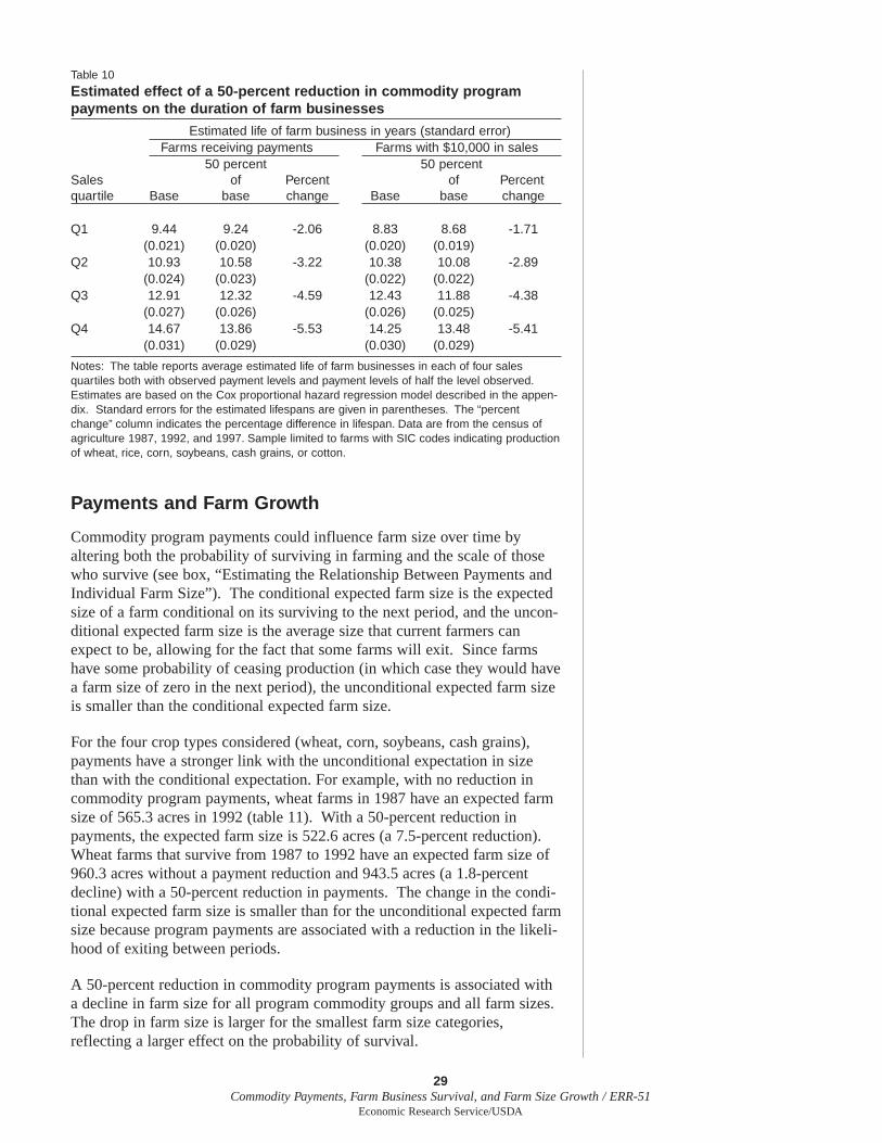
Payments and Farm Growth
Commodity program payments could influence farm size over time byaltering both the probability of surviving in farming and the scale of thosewho survive (see box, “Estimating the Relationship Between Payments andIndividual Farm Size”). The conditional expected farm size is the expectedsize of a farm conditional on its surviving to the next period, and the uncon-ditional expected farm size is the average size that current farmers canexpect to be, allowing for the fact that some farms will exit. Since farmshave some probability of ceasing production (in which case they would havea farm size of zero in the next period), the unconditional expected farm sizeis smaller than the conditional expected farm size.
For the four crop types considered (wheat, corn, soybeans, cash grains),payments have a stronger link with the unconditional expectation in sizethan with the conditional expectation. For example, with no reduction incommodity program payments, wheat farms in 1987 have an expected farmsize of 565.3 acres in 1992 (table 11). With a 50-percent reduction inpayments, the expected farm size is 522.6 acres (a 7.5-percent reduction).Wheat farms that survive from 1987 to 1992 have an expected farm size of960.3 acres without a payment reduction and 943.5 acres (a 1.8-percentdecline) with a 50-percent reduction in payments. The change in the condi-tional expected farm size is smaller than for the unconditional expected farmsize because program payments are associated with a reduction in the likeli-hood of exiting between periods.
A 50-percent reduction in commodity program payments is associated witha decline in farm size for all program commodity groups and all farm sizes.The drop in farm size is larger for the smallest farm size categories,reflecting a larger effect on the probability of survival.
29Commodity Payments, Farm Business Survival, and Farm Size Growth / ERR-51
Economic Research Service/USDA
Table 10
Estimated effect of a 50-percent reduction in commodity program payments on the duration of farm businesses
Estimated life of farm business in years (standard error)Farms receiving payments Farms with $10,000 in sales
50 percent 50 percentSales of Percent of Percentquartile Base base change Base base change
Q1 9.44 9.24 -2.06 8.83 8.68 -1.71(0.021) (0.020) (0.020) (0.019)
Q2 10.93 10.58 -3.22 10.38 10.08 -2.89(0.024) (0.023) (0.022) (0.022)
Q3 12.91 12.32 -4.59 12.43 11.88 -4.38(0.027) (0.026) (0.026) (0.025)
Q4 14.67 13.86 -5.53 14.25 13.48 -5.41(0.031) (0.029) (0.030) (0.029)
Notes: The table reports average estimated life of farm businesses in each of four sales quartiles both with observed payment levels and payment levels of half the level observed.Estimates are based on the Cox proportional hazard regression model described in the appen-dix. Standard errors for the estimated lifespans are given in parentheses. The “percentchange” column indicates the percentage difference in lifespan. Data are from the census ofagriculture 1987, 1992, and 1997. Sample limited to farms with SIC codes indicating productionof wheat, rice, corn, soybeans, cash grains, or cotton.

30Commodity Payments, Farm Business Survival, and Farm Size Growth / ERR-51
Economic Research Service/USDA
Table 11
Unconditional and conditional expected farm size
Unconditional expected Conditional expectedfarm size farm size
(farmland acres) (farmland acres)Type of farm in 50% reduction 50% reductionbeginning period Status quo in payments Status quo in payments Observations
Principal commodityWheat
1987-1992 565.3 522.6 960.3 943.5 37,0121992-1997 663.0 616.1 1059.3 1040.7 34,3521997-2002 703.9 653.5 1138.2 1118.3 32,312
Corn 1987-1992 214.6 198.5 361.9 355.6 86,8711992-1997 272.1 252.9 433.8 426.2 97,8251997-2002 304.9 283.4 485.6 477.1 98,576
Soybeans 1987-1992 166.4 153.7 288.6 283.5 87,4051992-1997 167.5 155.1 281.7 276.8 52,0351997-2002 222.4 206.5 360.0 353.7 68,700
Cash grains 1987-1992 368.6 344.2 556.3 546.5 88,0341992-1997 429.4 402.3 623.4 612.4 81,6041997-2002 491.8 460.9 711.1 698.6 81,224
Total farmland10-249 acres
1987-1992 57.0 51.9 118.1 116.1 149,5911992-1997 59.6 54.5 117.2 115.1 120,7251997-2002 61.4 56.2 119.9 117.8 121,427
250-499 acres1987-1992 200.3 185.0 343.5 337.5 60,8121992-1997 204.6 189.5 338.4 332.5 51,7881997-2002 204.6 189.6 339.1 333.2 53,998
500-999 acres1987-1992 419.4 389.9 662.3 650.7 51,2321992-1997 431.6 402.4 659.9 648.3 49,5981997-2002 431.0 401.7 662.6 651.0 52,922
1,000-1,999 acres1987-1992 822.3 766.5 1,261.4 1,239.2 25,9891992-1997 853.9 798.9 1,256.9 1,234.7 29,5591997-2002 858.9 803.2 1,270.9 1,248.5 34,306
2,000+ acres1987-1992 1,966.3 1,830.2 3,069.3 3,015.3 11,6981992-1997 2,029.7 1,897.0 3,025.8 2,972.5 14,1461997-2002 2,051.1 1,916.8 3,062.1 3,008.1 18,159
The table presents estimates of the unconditional and conditional farm size with and without implementation of a hypothetical policy thatreduces commodity program payments by 50 percent. Data are from the Census of Agriculture 1987, 1992, and 1997, and 2002. Sample limited to farms with SIC codes indicating production of wheat, corn, soybeans, or cash grains.
31Commodity Payments, Farm Business Survival, and Farm Size Growth / ERR-51
Economic Research Service/USDA
An estimation of the relationship between commodity programpayments and individual farm size must address the fact that thesample of farms that survive is not randomly selected from the popula-tion of all farms. Because it is only possible to observe the size offarms that survived, using an ordinary least squares regression to esti-mate the unconditional effect of commodity program payments onfarm size could produce inaccurate estimates if unobservable factorsare correlated with the likelihood of survival and farm growth. Forexample, if commodity program payments and an unobservable factorsuch as “farming ability” are both positively correlated with the proba-bility of survival and the rate of farm growth, then farmers with highability would be overrepresented among the sample of survivors.Within the sample of survivors, ability would be negatively correlatedwith commodity program payments: farmers would need high levels ofability to overcome low commodity program payments, and farmerswith low ability would need high payments to survive. Estimates ofthe effect of payment on farm size would therefore tend toward zero.To address this potential problem, the study uses a maximum likeli-hood approach to obtain consistent parameter estimates.
Data for this analysis are from the census of agriculture, 1987, 1992,1997, and 2002. To perform separate regression analyses for each typeof crop producer, this analysis limits the sample to producers special-izing in one of the four largest crops. The sample consists of 845,950farms that had at least 10 acres of land and were identified as primaryproducers of wheat, corn, soybeans, or “cash grains.” The data wereorganized into three panels: 1987-92, 1992-97, and 1997-2002. Theregression specification allowed for separate effects by SIC code, year,and size of operation. More details can be found in Key and Roberts(2007), which develops the empirical model used in the policy simula-tions reported here. Unlike Key and Roberts (2007), which was devel-oped before 2002 census data were available, results reported here arebased on data that include observations from the 2002 census.
Estimating the Relationship Between Payments and Individual Farm Size

Chapter 6
Summary and DiscussionFor the past several decades, crop production in the United States hasshifted to larger operations. The shares of cropland and farmland operatedby large-scale farms have steadily increased, while the shares operated bymedium-sized farms have declined. Many factors, including changes intechnology and factor prices, likely contributed to the increased concentra-tion of production. To what extent have commodity program paymentscontributed to this phenomenon?
This report uses data from five censuses to explore a series of empiricalrelationships between program payments and changes in farm structure. Ingeneral, the findings indicate a positive association between programpayments and subsequent increases in measures of farm concentration,survival, and growth. This association was maintained under differentmodel specifications. Across ZIP Code areas, cropland concentration grewfaster where beginning-period payments per acre were higher. Concentra-tion growth increased consistently as payment levels increased, and thispattern was similar in different time periods. This pattern persisted aftercontrolling for ZIP Code location, initial concentration, sales per croplandacre, and the ratio of cropland to other land uses.
The ZIP Code analysis was supplemented by analyses of farm businesssurvival and growth. These analyses compared the survival rates over timeof farms with high and low levels of payments as a share of sales, and esti-mated the relationship between payments and farm business survival ratewhile controlling for farm operator and operation characteristics. Findingsindicate a significant positive association between past commodity programpayments and farm survival rates, with and without controlling for otherfactors. Also, conditional on survival, payments are positively associatedwith growth in farm size.
Have Payments Made Farms Larger?
The findings of this report are consistent with the hypothesis that farmcommodity program payments influence structural change in agriculture.However, it is not possible to rule out other explanations for the observedassociations between payments and farm structure, despite efforts to controlfor factors that might cause spurious associations between programpayments and structural change. It is impossible to know whether factorsremain that have not been accounted for. This is a standard caveat to non-experimental studies that employ data observed in the natural world asopposed to data from a carefully controlled experiment (see footnote 4).Payment levels depend, to some extent, on farmers’ decisions to participatein government programs and on their production decisions. Hence, unob-served factors might affect both payment levels and farm structure, and biasestimates of the effect of payments.
32Commodity Payments, Farm Business Survival, and Farm Size Growth / ERR-51
Economic Research Service/USDA

For example, if variation in land quality is not adequately accounted for bythe controls, then this could be an alternative explanation for the findings inthe ZIP Code and farm-level analyses. Much of the local variation inpayments may be due to local variation in base acres and program yields.Areas with more base acres and higher program yields may also have supe-rior land quality. Technological change might be more scale-enhancing inareas with better land quality—for example, larger harvesters might be morefeasible in flatter and more productive regions. However, technologicalchange would also have to favor higher valued field crops relative to lowervalued crops (e.g., cotton over corn over wheat) to explain the payment-farm size relationship at a broader level. A technological effect of this kindwould seem coincidental, particularly because it would need to be associ-ated with payment levels in a consistent and gradual way in order to explainthe similar and steadily higher rates of concentration growth across the fivepayment quintiles.
Another possible noncausal explanation for the findings is that variation incommodity program payments per acre reflects differences in farmers’managerial abilities. That is, “better” farm managers are able to obtainhigher commodity program payments per acre due to their superior practicesand yields. But it seems unlikely that farming ability would significantlyinfluence variation in per-acre payments across farms, especially aftercontrolling for grower and operation characteristics (crop type, farm size,region, farmer age, farm organization, etc.). Because it is not possible tomeasure farmers’ ability to farm or obtain commodity program payments, itis not possible to measure the role of ability in the observed correlationbetween payments and farm size growth.
Reconciling the possible causal and noncausal explanations for the empir-ical findings of this study will require more research. For example, ifpayments facilitate growth in farm size by enhancing liquidity and loweringborrowing costs, then it should be possible to observe whether farmers whoreceive higher payments also receive better terms of credit from theirlenders. Or, if technological advances drove farm growth in areas with bothhigher land quality and higher payments, researchers should be able to iden-tify a set of technologies and show how they facilitated the whole range ofgreater farm sizes in different parts of the country. While technology hasclearly played a role in the concentration of production, less clear is howthese technologies might have acted to increase concentration in a patternaligned so closely with payment rates. Identifying a series of facts that arebroadly consistent with each other and with the observed pattern of farmsize growth will provide a better understanding of the pattern, and then,perhaps, draw out some deeper implications of farm policies.
33Commodity Payments, Farm Business Survival, and Farm Size Growth / ERR-51
Economic Research Service/USDA
ReferencesAudretsch, D. 1991. “New-Firm Survival and the Technological Regime,”
The Review of Economics and Statistics 73(3): 441-450.
Atwood, J., M. Watts, and A. Baquet. 1996. “An Examination of the Effectsof Price Supports and Federal Crop Insurance Upon the EconomicGrowth, Capital Structure, and Financial Survival of Wheat Growers inthe Northern High Plains,” American Journal of Agricultural Economics78 (Feb.): 212-224
Barry, P.J., R.W. Bierlen, and N.L. Sotomayor. 2000. “Financial Structure ofFarm Business under Imperfect Capital Markets,” American Journal ofAgricultural Economics 82(4) (Nov.): 427-35.
Bates, T. 1990. “Entrepreneur Human Capital Inputs and Small BusinessLongevity,” The Review of Economics and Statistics 72(4): 551-559
Bierlen, R., and A.M. Featherstone. 1998. “Fundamental Q, Cash Flow, andInvestment: Evidence from Farm Panel Data,” Review of Economics andStatistics 80 (Aug.): 427-35.
Claassen, R., V. Breneman, S. Bucholtz, A. Cattaneo, R. Johansson, and M.Morehart. 2004. Environmental Compliance in U.S. Agricultural Policy:Past Performance and Future Potential. U.S. Department of Agriculture,Economic Research Service, AER-832, May.
Cox, D.R. 1972. “Regression Models and Life-Tables (with Discussion),”Journal of the Royal Statistical Society, Series B 34: 187-220.
Cox, D.R. 1975. “Partial Likelihood,” Biometrika 62(2): 269-276.
Disney, R., J. Haskel, and Y. Heden. 2003. “Entry, Exit, and EstablishmentSurvival in UK Manufacturing,” Journal of Industrial Economics 51(1):91-112.
Dixon, B.L., N. Ma, B.L. Ahrendsen, L. Settlage, and J. Stam. 2004.“Factors Affecting State-Level Chapter 12 Filing Rates: A Panel DataModel,” Emory Bankruptcy Developments Journal 20(2): 401-426.
Evans, D. 1987a. “The Relationship between Firm Growth, Size, and Age:Estimates for 100 Manufacturing Industries,” Journal of IndustrialEconomics 35(June): 567-581.
_____. 1987b. “Tests of Alternative Theories of Firm Growth,” Journal ofPolitical Economy 95(Aug.): 657-674.
Evans, D., and B. Jovanovic. 1989. “An Estimated Model ofEntrepreneurial Choice under Liquidity Constraints,” Journal of PoliticalEconomy 97(4): 808-827
Goodwin, Barry K., A. Mishra, and F. Ortalo-Magne. 2003. “What’sWrong with Our Models of Agricultural Land Values?” AmericanJournal of Agricultural Economics 85(3): 744-752.
Hallam, A. 1993. “Empirical Studies of Size, Structure, and Efficiency inAgriculture,” Size, Structure, and the Changing Face of AmericanAgriculture, A. Hallam (ed.). Boulder, CO: Westview Press, pp. 204-31.
34Commodity Payments, Farm Business Survival, and Farm Size Growth / ERR-51
Economic Research Service/USDA

Holtz-Eakin, D., D. Joulfaian, and H. Rosen. 1994. “Sticking it Out:Entrepreneurial Survival and Liquidity Constraints,” Journal of PoliticalEconomy 102(1): 53-75.
Hoppe, R.A., and P. Korb. 2006. Understanding U.S. Farm Exits. U.S.Department of Agriculture, Economic Research Service. ERR-21. June.
Hubbard, R.G. 1998. “Capital-Market Imperfections and Investment,”Journal of Economic Literature 36 (March): 193-225.
Hubbard, R.G. and A.K. Kashyap. 1992. “Internal Net Worth and theInvestment Process: An Application to U.S. Agriculture,” Journal ofPolitical Economy 100(3) (June): 506-34.
Huffman, W. E., and R. E. Evenson. 2001. “Structural and ProductivityChange in U.S. Agriculture 1950-1982,” Agricultural Economics 24(2):127-147.
Kalbfleisch, J.D., and R.L. Prentice. 1980. The Statistical Analysis ofFailure Time Data, New York: John Wiley and Sons, Inc.
Key, N., and M.J. Roberts. 2007. “Commodity Program Payments andStructural Change in Agriculture,” Journal of Agricultural and ResourceEconomics. Vol. 32, No. 2 (Aug.): 330-348.
Key, N., and M.J. Roberts 2006. “Commodity Program Payments and FarmBusiness Survival,” American Journal of Agricultural Economics. 88(2)(May): 382-392.
Key, N., and M.J. Roberts. 2005. “Financial Market Imperfections andStructural Change in Agriculture,” Focus on Agricultural Economics Ami R. Bellows (ed.). New York: Nova Science Publishers, Inc.
Kimhi, A., and R. Bollman. 1999. “Family Farm Dynamics in Canada andIsrael: The Case of Farm Exits,” Agricultural Economics 21(1): 69-79.
Kislev, Y., and W. Peterson. 1983. “Prices, Technology, and Farm Size,”Journal of Political Economy 90(3) (June): 578-595.
Leathers, H. 1992. “The Market for Land and the Impact of Farm Programson Farm Numbers,” American Journal of Agricultural Economics 74:291-98.
Lopez, R. 1984. “Estimating Labor Supply and Production Decisions ofSelf-Employed Farm Producers,” European Economic Review 24: 61-82.
Lubowski, R., M. Vesterby, S. Bucholtz, A. Baez, and M. Roberts. 2006.Major Uses of Land in the United States, 2002. EIB-14. U.S. Departmentof Agriculture, Economic Research Service. May.
MacDonald, J., R. Hoppe, and D. Banker. 2005. “Changing Farm Size andthe Distribution of Farm Payments,” Amber Waves 3(1), U.S. Departmentof Agriculture, Economic Research Service, Feb.
Mata, J., P. Portugal, and P. Guimaraes. 1995. “The Survival of New Plants:Start-up Conditions and Post-entry Evolution,” International Journal ofIndustrial Organization 13: 459-481.
35Commodity Payments, Farm Business Survival, and Farm Size Growth / ERR-51
Economic Research Service/USDA
Mishra, A., H. El-Osta, M. Morehart, J. Johnson, and J. Hopkins. 2002.Income, Wealth, and the Economic Well-Being of Farm Households. U.S.Department of Agriculture, Economic Research Service, AER-812, July.
Morrison Paul, C.J., and R. Nehring. 2005. “Product diversification, pro-duction systems, and economic performance in U.S. agricultural produc-tion,” Journal of Econometrics 126: 525-48.
Morrison Paul, C.J., R. Nehring, D. Banker, and A. Somwaru. 2004. “ScaleEconomies and Efficiency in U.S. Agriculture: Are Traditional FarmsHistory?” Journal of Productivity Analysis 22: 185-205
Nelson, E.B. 2002. “Payment Limitations Amendment Passes Senate:Nelson Co-Sponsored Amendment Restores Equity to Farm Payments,”Press release, February 7. http://bennelson.senate.gov/2002/releases/paymentlimits.htm
Ravallion, M. 2005. “Evaluating Anti-Poverty Programs,” World BankPolicy Research Working Paper 3625, June.
Roberts, M.J., B. Kirwan, and J. Hopkins. 2003. “The Incidence ofGovernment Program Payments on Agricultural Land Rents: TheChallenges of Identification,” American Journal of AgriculturalEconomics 85(3): 762-769.
Roberts, M.J., N. Key, and E. O’Donoghue. 2006. “Estimating the Incidenceof Moral Hazard in Crop Insurance Using Administrative Data,” Reviewof Agricultural Economics. 2006 ASSA Meetings Proceedings Paper.
Roberts, M.J., and N. Key. “Commodity Program Payments and FarmlandConcentration.” Selected paper, 2006 AAEA Annual Meetings, LongBeach, CA.
Roberts, M.J., and N. Key. 2002. “Risk and Liquidity Constraints in U.S.Agriculture,” A Comprehensive Assessment of the Role of Risk in U.S.Agriculture, Just and Pope (eds.). Dordrecht and London: KluwerAcademic.
Shepard, L., and R. Collins. 1982. “Why Do Farmers Fail? FarmBankruptcies 1910-78,” American Journal of Agricultural Economics 64:609-615.
Sumner, D.A., and J. D. Leiby. 1987. “An Econometric Analysis of theEffects of Human Capital on Size and Growth among Dairy Farms,”American Journal of Agricultural Economics 69(2): 465-70
Taylor, M.P. 1999. “Survival of the Fittest? An Analysis of Self-Employment Duration in Britain,” Economic Journal 109(454): 140-55.
36Commodity Payments, Farm Business Survival, and Farm Size Growth / ERR-51
Economic Research Service/USDA

Tweeten, L. 1993. “Government Commodity Program Impacts on FarmNumbers,” Size, Structure and the Changing Face of AmericanAgriculture, A. Hallam (ed.), Boulder, CO: Westview Press.
U.S. Department of Agriculture. Historical commodity specific yearbooks(various years). Economic Research Service. www.ers.usda.gov
U.S. Department of Agriculture. National Agricultural Statistics Service.1997. “General Terms,” http://www.nass.usda.gov/census/census97/general.pdf
U.S. Department of Agriculture. Economic Research Service. 2003.“Statistical Indicators,” Agricultural Outlook July.http://www.ers.usda.gov/publications/AgOutlook/AOTables/2003/07Jul/AoTab35.xls
U.S. Department of Agriculture. 2003. Report of the Commission on theApplication of Payment Limitations for Agriculture. Submitted inResponse to Section 1605, Farm Security and Rural Investment Act of2002. Prepared by the Commission on the Application of PaymentLimitations for Agriculture. Office of the Chief Economist, USDA. Aug.
U.S. Department of Agriculture. 2006. “Risk Management.” A 2007 FarmBill Theme Paper released by the Secretary of Agriculture. Seehttp://www.usda.gov/documents/Farmbill07riskmgmtrev.pdf .
U.S. Department of Agriculture. Economic Research Service. 2007. Farmand Commodity Policy: Commodity Program Payments and the FarmSector. http://www.ers.usda.gov/Briefing/FarmPolicy/gov-pay.htm
Venables, W.N., and B.D. Ripley. 2002. Modern Applied Statistics with S,Fourth Edition. New York: Springer-Verlag.
Weiss, C. 1999. “Farm Growth and Survival: Econometric Evidence forIndividual Farms in Upper Austria,” American Journal of AgriculturalEconomics 81(Feb.): 103-116.
Williams-Derry, C., and K. Cook. 2000. “Green Acres: How Taxpayers areSubsidizing the Demise of the Family Farm.” Environmental WorkingGroup, Washington, DC. April
Wimberley, Ronald C. 2006. “What is a Farm, and Why Does it Matter?”Proceedings of the National Small Farm Conference, Sep., Nashville, TN.(http://www.nal.usda.gov/afsic/nsfc/2iif3.htm)
Zepeda, L. 1995. “Asymmetry and Nonstationarity in the Farm SizeDistribution of Wisconsin Milk Producers: An Aggregate Analysis,”American Journal of Agricultural Economics 77(4): 837-852.
37Commodity Payments, Farm Business Survival, and Farm Size Growth / ERR-51
Economic Research Service/USDA
The study estimated the link between payments and concentration growth inseveral ways, both with and without controls. Results were similar in allcases. This appendix provides more detail about the methods used to deriveresults in tables 6 and 7 and figures 6 and 7, as well as some additionalresults obtained using different estimation procedures.
For the estimates reported in table 6, concentration is defined as theweighted-median cropland area in each ZIP Code (the acres of cropland onthe farm for which half the cropland acreage occurs on farms with morecropland and half on farms with less). For each ZIP Code and panel, thepercentage change in concentration is calculated as 100 times the change inconcentration divided by average concentration in the two years considered.The long panels calculate the percentage change between 1987 and 2002.Payments per acre in each ZIP Code are calculated by dividing totalpayments in the beginning year by total cropland. ZIP Codes with nopayments comprised one payment group and those with positive paymentswere classified into five quintiles, each with the same number of ZIP Codes.The payment-per-acre cutoffs are different in the different panels becausepayments vary across years. The cutoffs were chosen so as to have the samenumber of ZIP Codes in each quintile with positive payments. For the longpanels, the payment groups were constructed using payments per acre in1987. Because ZIP Codes receive different payment levels in different yearsand are sometimes classified into different payment groups in differentpanels, the percentage change for the long panel does not equal the sum ofthe individual panels.
The sample of ZIP Codes in the analysis is somewhat less than the popula-tion of ZIP Codes in the census of agriculture. ZIP Codes were droppedfrom the analysis if (1) less than three farms returned census forms in any ofthe four censuses examined; (2) if the ZIP Code reported no cropland in anyof the panel years; (3) if commodity program payments per acre, the ratio ofcropland area to ZIP Code area, or the ratio of crop sales to cropland areawere in the top 2 percent of all ZIP Codes. The extreme observations wereomitted from the analysis due to the highly skewed distributions of thesevariables. For example, some ZIP Codes may have extremely highpayment-to-cropland ratios if there are very few acres of cropland, but amodest level of payments, perhaps as a result of historical plantings. Afteromitting these observations, the analyses include 21,524 ZIP Codes.
Results reported in table 7 (with controls) are derived from estimation ofgeneralized additive models with the form:
Δci = Xiβ + f(xi,yi) + gc(c0i) + ga(a0i) + gs(s0i) + εi
where subscript i (omitted below to simplify notation) indexes ZIP Codes,c0 denotes concentration in the beginning year, Δc is the percent change inconcentration ( (c1- c0)/ ½(c1 + c0) ), X is a matrix of indicator variablesdenoting payment-per-acre categories (one column of each row equals 1 andthe others equal 0), β is a vector of payment-category effects, f(x,y) is a
38Commodity Payments, Farm Business Survival, and Farm Size Growth / ERR-51
Economic Research Service/USDA
Appendix: Estimating the Link Between Paymentsand Concentration Growth
smooth function of locations (x, y) of ZIP Code centroids, gc(c0) is a smoothfunction of beginning-year concentration (c0), ga(a0) is a smooth function ofthe ratio of cropland area to ZIP Code area in the beginning year (a0), gs(s0)is a smooth function of crop sales per acre of cropland (s0), and ε is arandom error. For the long panels, Δc is the sum of percentage changes inconcentration in the three individual panels, and c0, a0, and s0 are theaverage of values from 1987, 1992, and 1997.
The critical assumption is that, conditional on controls for location, begin-ning-year concentration, beginning-year ratio of cropland to ZIP Code area,and beginning-year crop sales per cropland acre, payments per acre are notcorrelated with other, unobserved factors affecting concentration growth(εi).
The smooth functions were estimated using “loess,” short for “local polyno-mial regression,” which fits the smooth functions by estimating polynomialfunctions using points local to each fitted point, with local points weightedmore heavily than further points. The smooth functions are estimated jointlywith β using a Gauss-Seidel backfitting method, as described and imple-mented by Hastie. The software package used was the public domainpackage ‘R’ with the ‘gam’ package written by Hastie (www.r-project.org).See this reference for more details about the procedure.
The key modeling decision concerns the share of points considered local toeach fitted point on the smooth functions. For the models, each point alongthe smooth functions was estimated using 5 percent of the ZIP Codes,which is the smallest share that was computationally feasible for the two-dimensional spatial surface using the hardware and software. Summaries ofthe models with payment quintiles are reported in appendix table A1,excluding the parametric components reported in table 7.
Appendix table A2 reports a series of alternative long-panel estimates thatillustrate the general robustness of the link between payment levels andconcentration growth. The first set of estimates in the table are ordinaryleast squares (OLS) estimates with the control functions f(), gc(), ga(), andgs() approximated using orthogonal polynomials of varying orders. Thetable reports the estimated payment-group effects conditional on the polyno-mial controls. The orders of single-variable polynomials (gc(), ga(), andgs()) are the given in the first column; the orders of the two-variable spatialfunction f() are twice the number in the first column. Results can becompared to the unadjusted estimates (without controls), replicated fromtable 6 at the top of the table.
The second set of estimates in table A2 are robust regressions, or M esti-mates, fitted using iterated re-weighted least squares (IWLS). The weightsare derived from penalty functions that reduce or eliminate the influence ofoutliers. The estimates are derived using Tukey’s biweight proposal. Theestimates were implemented using the public domain software “R” and the“MASS” package written by Venables and Ripley. More details can befound in Venables and Ripley and in the R documentation for the “rlm”function in the MASS package. Estimates were derived using the defaultmethod for the “MM” option. Robust methods are more computationallyexpensive than OLS, which limits the order of polynomials to 10 for boththe single variable and two-variable spatial controls.
39Commodity Payments, Farm Business Survival, and Farm Size Growth / ERR-51
Economic Research Service/USDA

40Commodity Payments, Farm Business Survival, and Farm Size Growth / ERR-51
Economic Research Service/USDA
Table A1
Summary of generalized additive model estimates
Non-parametricdegrees of F-
Panel Factor freedom value Goodness of fit
Spatial surface (x,y) 73.0 16.3Beginning-year concentration (c0) 35.5 58.0
Ratio of cropland to ZIP Code area (a0) 35.8 10.7Crop sales per acre of cropland (s0) 36.3 2.2
Spatial surface (x,y) 72.9 13.4Beginning-year concentration (c0) 35.2 65.0
Ratio of cropland to ZIP Code area (a0) 35.7 11.4Crop sales per acre of cropland (s0) 36.1 4.5
Spatial surface (x,y) 71.4 13.1Beginning-year concentration (c0) 35.2 66.5
Ratio of cropland to ZIP Code area (a0) 35.6 11.0Crop sales per acre of cropland (s0) 35.7 3.2
Spatial surface (x,y) 88.9 23.6Beginning-year concentration (c0) 45.5 42.9
Ratio of cropland to ZIP Code area (a0) 45.5 13.3Crop sales per acre of cropland (s0) 46.0 4.7
Notes: Estimates and standard errors for the parametric components of the models (the payment group factors) are reported in table 6. All F-tests for nonparametrically estimated smooth functions are statistically significant with at least 0.1-percent confidence.
Croplandconcentration
1987-1992
Cropland concentration
1992-1997
Cropland concentration
1997-2002
Cropland concentration
Long panel1987-2002
Adj. R2 = 0.153Est. VAR(ε) = 0.281
Adj. R2 = 0.130Est. VAR(ε) = 0.294
Adj. R2 = 0.135Est. VAR(ε) = 0.348
Adj. R2 = 0.212Est. VAR(ε) = 0.49
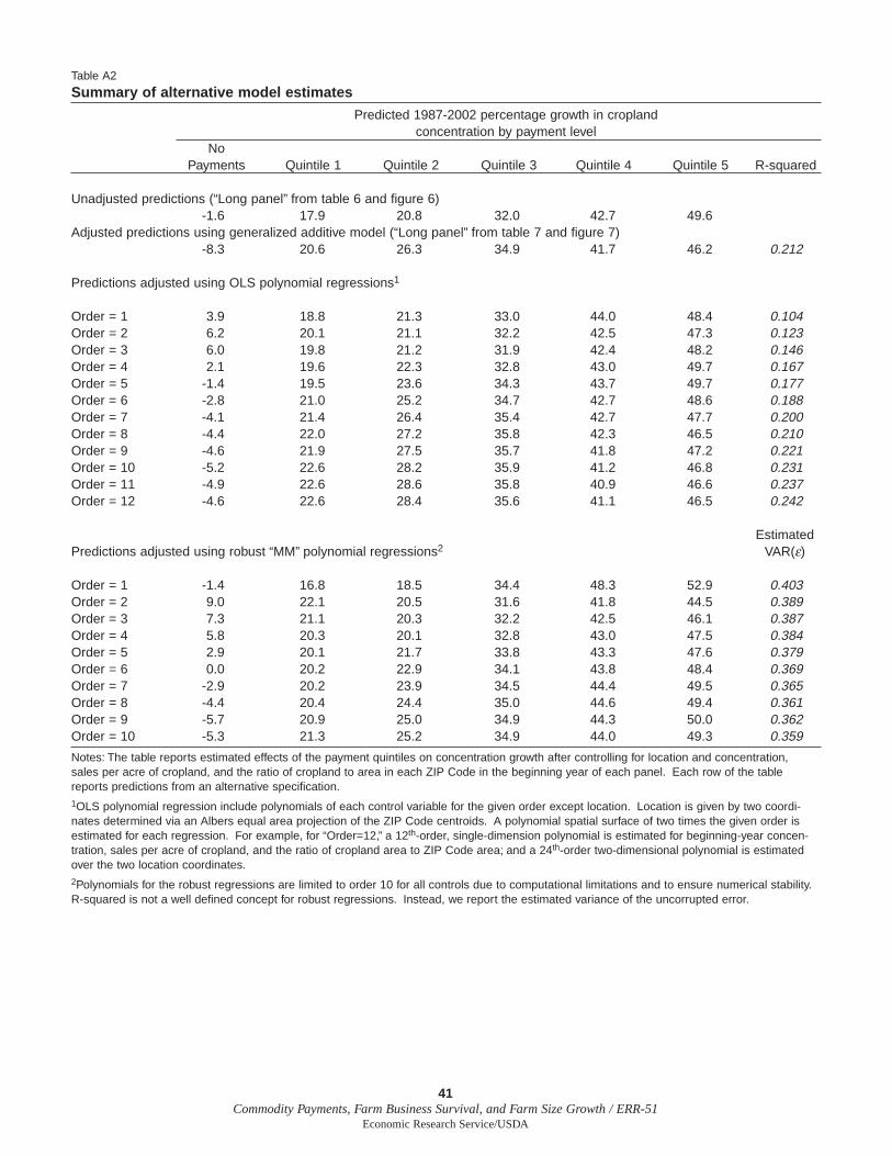
41Commodity Payments, Farm Business Survival, and Farm Size Growth / ERR-51
Economic Research Service/USDA
Table A2
Summary of alternative model estimates
Predicted 1987-2002 percentage growth in cropland concentration by payment level
NoPayments Quintile 1 Quintile 2 Quintile 3 Quintile 4 Quintile 5 R-squared
Unadjusted predictions (“Long panel” from table 6 and figure 6)-1.6 17.9 20.8 32.0 42.7 49.6
Adjusted predictions using generalized additive model (“Long panel” from table 7 and figure 7)-8.3 20.6 26.3 34.9 41.7 46.2 0.212
Predictions adjusted using OLS polynomial regressions1
Order = 1 3.9 18.8 21.3 33.0 44.0 48.4 0.104Order = 2 6.2 20.1 21.1 32.2 42.5 47.3 0.123Order = 3 6.0 19.8 21.2 31.9 42.4 48.2 0.146Order = 4 2.1 19.6 22.3 32.8 43.0 49.7 0.167Order = 5 -1.4 19.5 23.6 34.3 43.7 49.7 0.177Order = 6 -2.8 21.0 25.2 34.7 42.7 48.6 0.188Order = 7 -4.1 21.4 26.4 35.4 42.7 47.7 0.200Order = 8 -4.4 22.0 27.2 35.8 42.3 46.5 0.210Order = 9 -4.6 21.9 27.5 35.7 41.8 47.2 0.221Order = 10 -5.2 22.6 28.2 35.9 41.2 46.8 0.231Order = 11 -4.9 22.6 28.6 35.8 40.9 46.6 0.237Order = 12 -4.6 22.6 28.4 35.6 41.1 46.5 0.242
Estimated Predictions adjusted using robust “MM” polynomial regressions2 VAR(ε)
Order = 1 -1.4 16.8 18.5 34.4 48.3 52.9 0.403Order = 2 9.0 22.1 20.5 31.6 41.8 44.5 0.389Order = 3 7.3 21.1 20.3 32.2 42.5 46.1 0.387Order = 4 5.8 20.3 20.1 32.8 43.0 47.5 0.384Order = 5 2.9 20.1 21.7 33.8 43.3 47.6 0.379Order = 6 0.0 20.2 22.9 34.1 43.8 48.4 0.369Order = 7 -2.9 20.2 23.9 34.5 44.4 49.5 0.365Order = 8 -4.4 20.4 24.4 35.0 44.6 49.4 0.361Order = 9 -5.7 20.9 25.0 34.9 44.3 50.0 0.362Order = 10 -5.3 21.3 25.2 34.9 44.0 49.3 0.359
Notes: The table reports estimated effects of the payment quintiles on concentration growth after controlling for location and concentration, sales per acre of cropland, and the ratio of cropland to area in each ZIP Code in the beginning year of each panel. Each row of the tablereports predictions from an alternative specification.1OLS polynomial regression include polynomials of each control variable for the given order except location. Location is given by two coordi-nates determined via an Albers equal area projection of the ZIP Code centroids. A polynomial spatial surface of two times the given order isestimated for each regression. For example, for “Order=12,” a 12th-order, single-dimension polynomial is estimated for beginning-year concen-tration, sales per acre of cropland, and the ratio of cropland area to ZIP Code area; and a 24th-order two-dimensional polynomial is estimated over the two location coordinates.2Polynomials for the robust regressions are limited to order 10 for all controls due to computational limitations and to ensure numerical stability.R-squared is not a well defined concept for robust regressions. Instead, we report the estimated variance of the uncorrupted error.