communication avoiding lu and qr factorizations · communication avoiding lu and qr factorizations...

Communication avoiding LU and QR factorizations

Laura Grigori ALPINES

INRIA Rocquencourt - LJLL, UPMC On sabbatical at UC Berkeley

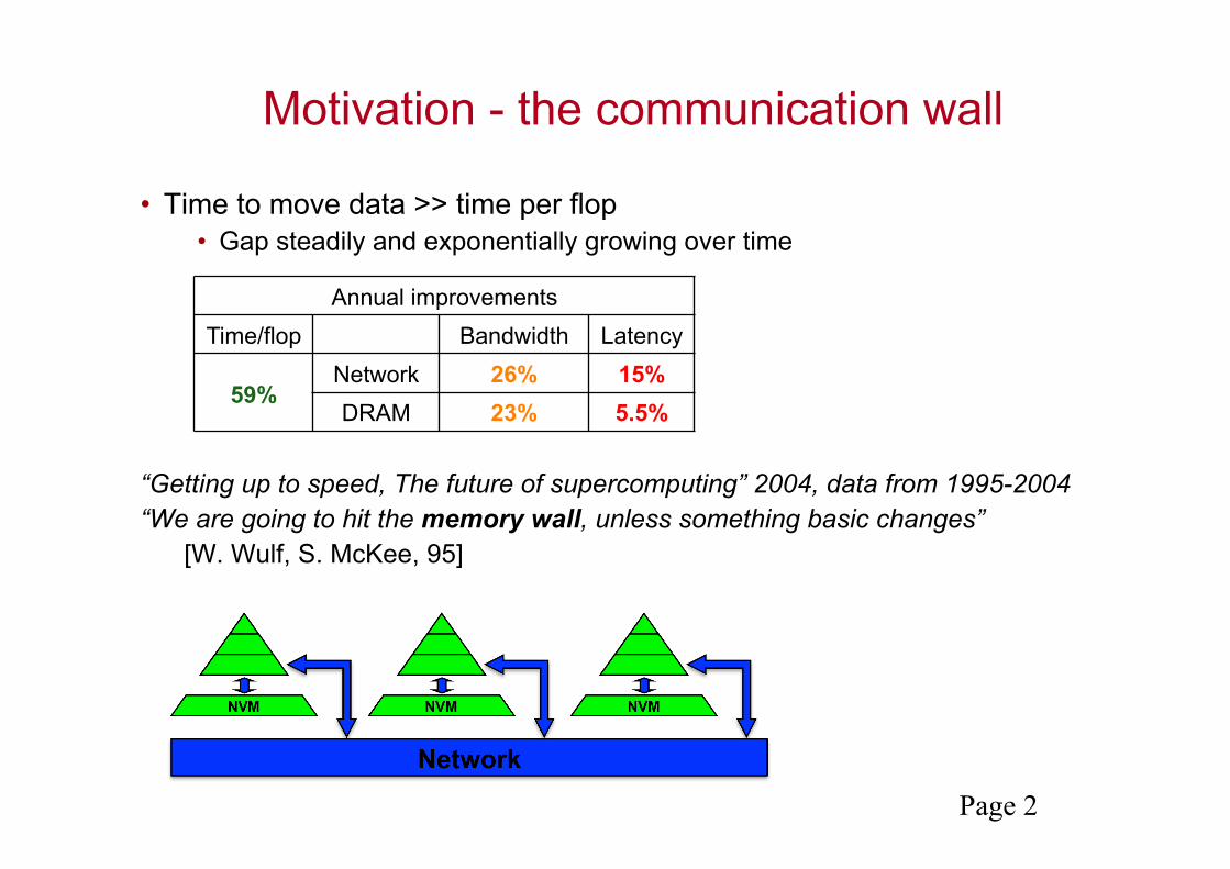
Motivation - the communication wall

•  Time to move data >> time per flop •  Gap steadily and exponentially growing over time

“Getting up to speed, The future of supercomputing” 2004, data from 1995-2004 “We are going to hit the memory wall, unless something basic changes” [W. Wulf, S. McKee, 95]

Annual improvements Time/flop Bandwidth Latency

59% Network 26% 15%

DRAM 23% 5.5%

Compelling numbers (1)

DRAM bandwidth: •  Mid 90’s ~ 0.2 bytes/flop – 1 byte/flop •  Past few years ~ 0.02 to 0.05 bytes/flop

DRAM latency: •  DDR2 (2007) ~ 120 ns 1x •  DDR4 (2014) ~ 45 ns 2.6x in 7 years •  Stacked memory ~ similar to DDR4

Time/flop •  2006 Intel Yonah ~ 2GHz x 2 cores (32 GFlops/chip) 1x •  2015 Intel Haswell ~2.3GHz x 16 cores (588 GFlops/chip) 18x in 9 years

Source: J. Shalf, LBNL

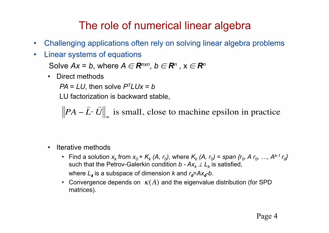
The role of numerical linear algebra •  Challenging applications often rely on solving linear algebra problems •  Linear systems of equations Solve Ax = b, where A ∈ Rnxn, b ∈ Rn , x ∈ Rn

•  Direct methods PA = LU, then solve PTLUx = b LU factorization is backward stable,

•  Iterative methods •  Find a solution xk from x0 + Kk (A, r0), where Kk (A, r0) = span {r0, A r0, …, Ak-1 r0}

such that the Petrov-Galerkin condition b - Axk ⊥ Lk is satisfied, where Lk is a subspace of dimension k and r0=Ax0-b. •  Convergence depends on and the eigenvalue distribution (for SPD

matrices).

€

PA −) L ⋅

) U

∞ is small, close to machine epsilon in practice

€

κ(A)

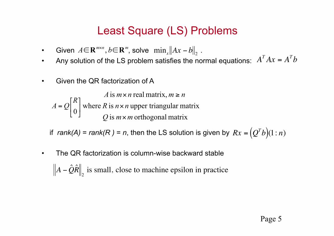
Least Square (LS) Problems •  Given , solve . •  Any solution of the LS problem satisfies the normal equations:

•  Given the QR factorization of A

if rank(A) = rank(R ) = n, then the LS solution is given by

•  The QR factorization is column-wise backward stable

mnm bA RR ∈∈ × ,

€

minx Ax − b 2

€

AT Ax = ATb

matrix orthogonal is matrix ngular upper tria is

matrix, real is where

0mmQnnR

nmnmAR

QA×

×

≥×

⎥⎦

⎤⎢⎣

⎡=

€

Rx = QTb( )(1: n)

€

A − ˆ Q ̂ R 2 is small, close to machine epsilon in practice

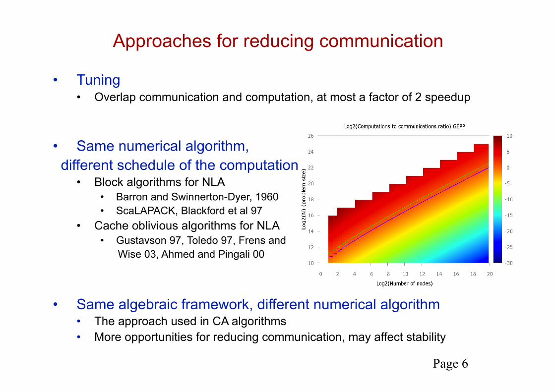
Approaches for reducing communication

•  Tuning •  Overlap communication and computation, at most a factor of 2 speedup

•  Same numerical algorithm, different schedule of the computation

•  Block algorithms for NLA •  Barron and Swinnerton-Dyer, 1960 •  ScaLAPACK, Blackford et al 97

•  Cache oblivious algorithms for NLA •  Gustavson 97, Toledo 97, Frens and Wise 03, Ahmed and Pingali 00

•  Same algebraic framework, different numerical algorithm •  The approach used in CA algorithms •  More opportunities for reducing communication, may affect stability

Motivation

•  The communication problem needs to be taken into account higher in the computing stack

•  A paradigm shift in the way the numerical algorithms are devised is required

•  Communication avoiding algorithms - a novel perspective for numerical linear algebra •  Minimize volume of communication •  Minimize number of messages •  Minimize over multiple levels of memory/parallelism •  Allow redundant computations (preferably as a low order term)

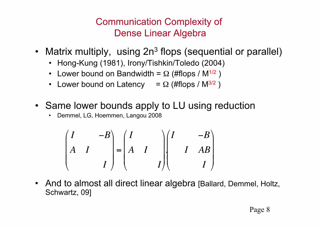
Communication Complexity of Dense Linear Algebra

•  Matrix multiply, using 2n3 flops (sequential or parallel) •  Hong-Kung (1981), Irony/Tishkin/Toledo (2004) •  Lower bound on Bandwidth = Ω (#flops / M1/2 ) •  Lower bound on Latency = Ω (#flops / M3/2 )

€

I −BA I

I

⎛

⎝

⎜ ⎜ ⎜

⎞

⎠

⎟ ⎟ ⎟

=

IA I

I

⎛

⎝

⎜ ⎜ ⎜

⎞

⎠

⎟ ⎟ ⎟ .I −B

I ABI

⎛

⎝

⎜ ⎜ ⎜

⎞

⎠

⎟ ⎟ ⎟

•  Same lower bounds apply to LU using reduction •  Demmel, LG, Hoemmen, Langou 2008

•  And to almost all direct linear algebra [Ballard, Demmel, Holtz, Schwartz, 09]

Sequential algorithms and communication bounds

Algorithm Minimizing #words (not #messages)

Minimizing #words and #messages

Cholesky

LU

QR

RRQR

•  Only several references shown for block algorithms (LAPACK), cache-oblivious algorithms and communication avoiding algorithms •  CA algorithms exist also for SVD and eigenvalue computation

[Gustavson, 97] [Ahmed, Pingali, 00]

[LG, Demmel, Xiang, 08] [Khabou, Demmel, LG, Gu, 12]

uses tournament pivoting

[Frens, Wise, 03], 3x flops [Demmel, LG, Hoemmen, Langou, 08]

[Ballard et al, 14] [Demmel, LG, Gu, Xiang 11]

uses tournament pivoting, 3x flops

LAPACK

LAPACK (few cases) [Toledo,97], [Gustavson, 97]

both use partial pivoting

LAPACK (few cases) [Elmroth,Gustavson,98]

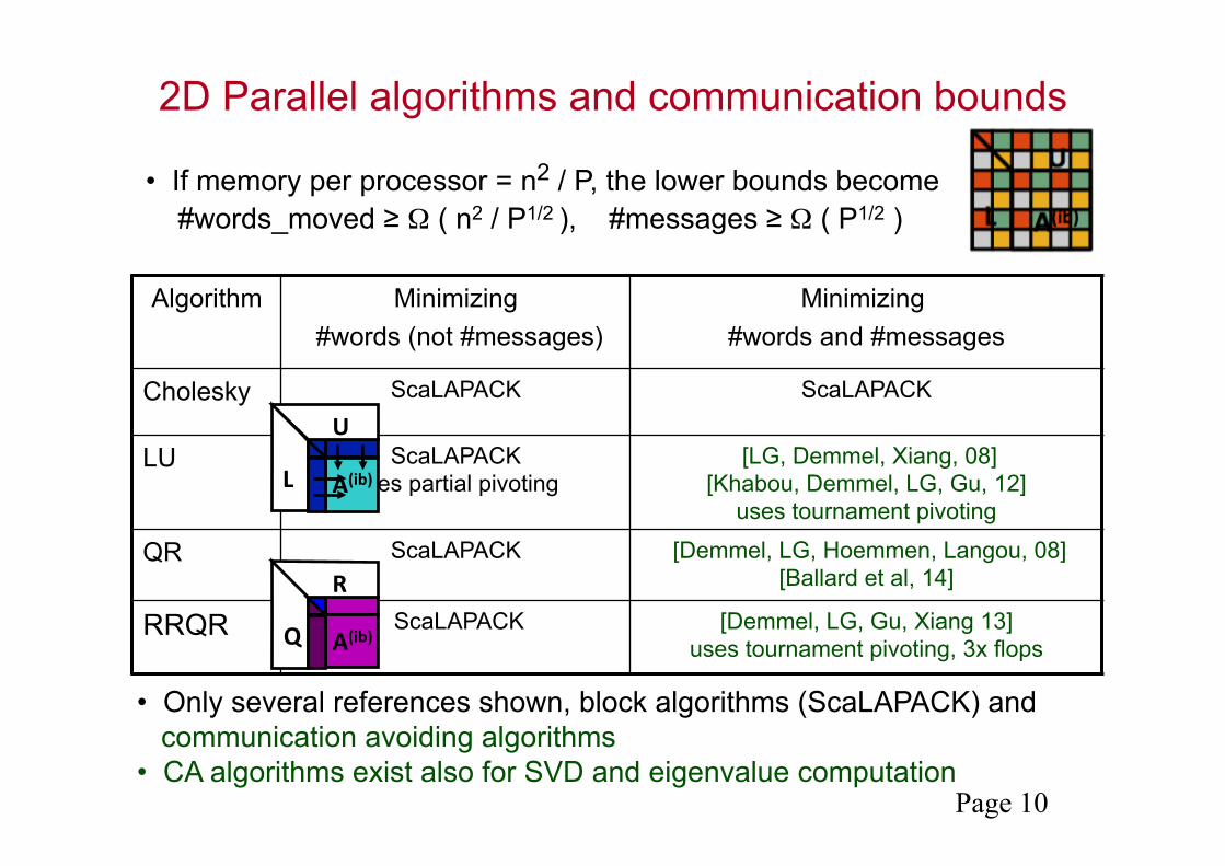
2D Parallel algorithms and communication bounds

Algorithm Minimizing #words (not #messages)

Minimizing #words and #messages

Cholesky ScaLAPACK ScaLAPACK

LU ScaLAPACK uses partial pivoting

[LG, Demmel, Xiang, 08] [Khabou, Demmel, LG, Gu, 12]

uses tournament pivoting

QR ScaLAPACK [Demmel, LG, Hoemmen, Langou, 08] [Ballard et al, 14]

RRQR ScaLAPACK [Demmel, LG, Gu, Xiang 13] uses tournament pivoting, 3x flops

•  Only several references shown, block algorithms (ScaLAPACK) and communication avoiding algorithms •  CA algorithms exist also for SVD and eigenvalue computation

•  If memory per processor = n2 / P, the lower bounds become #words_moved ≥ Ω ( n2 / P1/2 ), #messages ≥ Ω ( P1/2 )

L

U

A(ib)

Q

R

A(ib)

Scalability of communication optimal algorithms •  2D communication optimal algorithms, M = 3⋅n2/P

(matrix distributed over a P1/2-by- P1/2 grid of processors) TP = O ( n3 / P ) γ + Ω ( n2 / P1/2 ) β + Ω ( P1/2 ) α •  Isoefficiency: n3 ∝ P1.5 and n2 ∝ P •  For GEPP, n3 ∝ P2.25 [Grama et al, 93]

•  3D communication optimal algorithms, M = 3⋅P1/3(n2/P) (matrix distributed over a P1/3-by- P1/3-by- P1/3 grid of processors)

TP = O ( n3 / P ) γ + Ω ( n2 / P2/3 ) β + Ω ( log(P) ) α •  Isoefficiency: n3 ∝ P and n2 ∝ P2/3

•  2.5D algorithms with M = 3⋅c⋅(n2/P), and 3D algorithms exist for matrix multiplication and LU factorization

•  References: Dekel et al 81, Agarwal et al 90, 95, Johnsson 93, McColl and Tiskin 99, Irony and Toledo 02, Solomonik and Demmel 2011

E - the ratio between execution time on a single processor and total execution time summed over P processors. Isoefficiency - how the amount of computation must scale with P to keep E constant.

2.5D algorithms for LU, QR •  Assume c>1 copies of data, memory per processor is M ≈ c⋅(n2/P)

•  For matrix multiplication •  The bandwidth is reduced by a factor of c1/2

•  The latency is reduced by a factor of c3/2 •  Perfect Strong Scaling regime, given P such that M = 3n2 /P T(cP) = T(P)/c

•  For LU, QR •  The bandwidth can be reduced by a factor of c1/2

•  But then the latency will increase by a factor of c1/2

•  Thm [Solomonik et al]: Perfect Strong Scaling impossible for LU, because

Latency*Bandwidth = Ω(n2) •  Conjecture: this applies to other factorizations as QR, RRQR, etc.

2.5D LU with and without pivoting

•  2.5D algorithms with M = 3⋅c⋅(n2/P), and 3D algorithms exist for matrix multiplication and LU factorization

•  References: Dekel et al 81, Agarwal et al 90, 95, Johnsson 93, McColl and Tiskin 99, Irony and Toledo 02, Solomonik and Demmel 2011 (data presented below)

0

20

40

60

80

100

NO-pivot 2D

NO-pivot 2.5D

CA-pivot 2D

CA-pivot 2.5D

Tim

e (

sec)

LU on 16,384 nodes of BG/P (n=131,072)

2X faster

2X faster

computeidle

communication

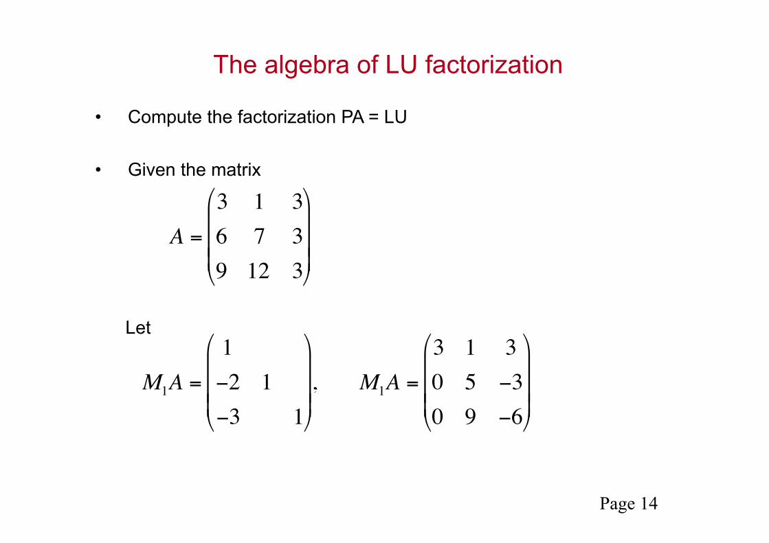
The algebra of LU factorization

•  Compute the factorization PA = LU

•  Given the matrix

Let

€

A =

3 1 36 7 39 12 3

⎛

⎝

⎜ ⎜ ⎜

⎞

⎠

⎟ ⎟ ⎟

€

M1A =

1−2 1−3 1

⎛

⎝

⎜ ⎜ ⎜

⎞

⎠

⎟ ⎟ ⎟ , M1A =

3 1 30 5 −30 9 −6

⎛

⎝

⎜ ⎜ ⎜

⎞

⎠

⎟ ⎟ ⎟

The need for pivoting •  For stability avoid division by small elements, otherwise ||A-LU||

can be large •  Because of roundoff error

•  For example

has an LU factorization if we permute the rows of A

•  Partial pivoting allows to bound all elements of L by 1.

€

A =

0 3 33 1 36 2 3

⎛

⎝

⎜ ⎜ ⎜

⎞

⎠

⎟ ⎟ ⎟

€

PA =

6 2 30 3 33 1 3

⎛

⎝

⎜ ⎜ ⎜

⎞

⎠

⎟ ⎟ ⎟

=

11

0.5 1

⎛

⎝

⎜ ⎜ ⎜

⎞

⎠

⎟ ⎟ ⎟

6 2 33 31.5

⎛

⎝

⎜ ⎜ ⎜

⎞

⎠

⎟ ⎟ ⎟

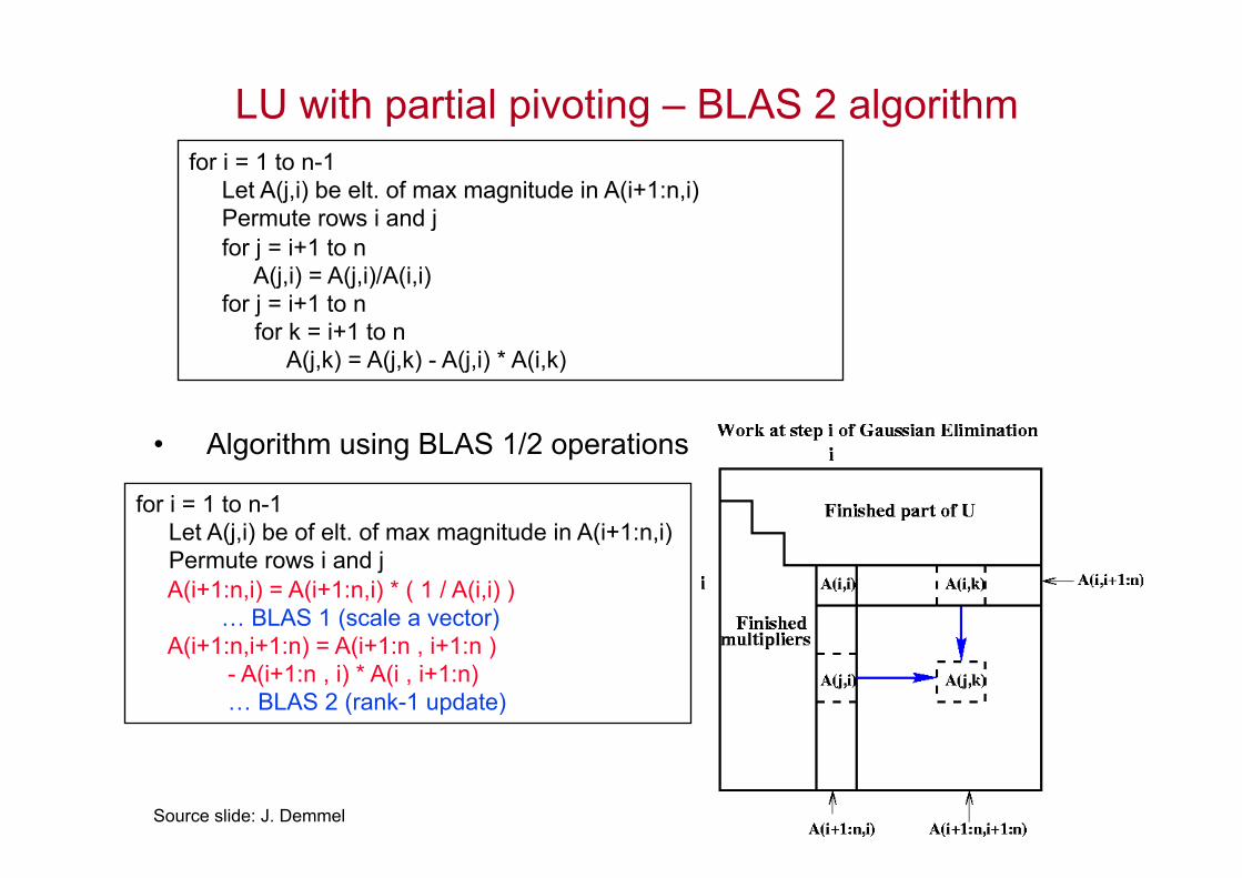
LU with partial pivoting – BLAS 2 algorithm

•  Algorithm using BLAS 1/2 operations

Source slide: J. Demmel

for i = 1 to n-1 Let A(j,i) be of elt. of max magnitude in A(i+1:n,i) Permute rows i and j A(i+1:n,i) = A(i+1:n,i) * ( 1 / A(i,i) ) … BLAS 1 (scale a vector) A(i+1:n,i+1:n) = A(i+1:n , i+1:n ) - A(i+1:n , i) * A(i , i+1:n) … BLAS 2 (rank-1 update)

for i = 1 to n-1 Let A(j,i) be elt. of max magnitude in A(i+1:n,i) Permute rows i and j for j = i+1 to n A(j,i) = A(j,i)/A(i,i) for j = i+1 to n for k = i+1 to n A(j,k) = A(j,k) - A(j,i) * A(i,k)

Block LU factorization – obtained by delaying updates

•  Matrix A of size nxn is partitioned as

•  The first step computes LU with partial pivoting of the first block:

•  The factorization obtained is:

•  The algorithm continues recursively on the trailing matrix A221

€

A =A11 A12

A21 A22

⎡

⎣ ⎢

⎤

⎦ ⎥ , where A11 is b × b

€

P1A11A21

⎛

⎝ ⎜

⎞

⎠ ⎟ =

L11L21

⎛

⎝ ⎜

⎞

⎠ ⎟ U11

€

P1A =L11

L21 In−b

⎛

⎝ ⎜

⎞

⎠ ⎟ U11 U12

A221

⎛

⎝ ⎜

⎞

⎠ ⎟ , where

U12 = L11−1A12

A221 = A22 − L21U12

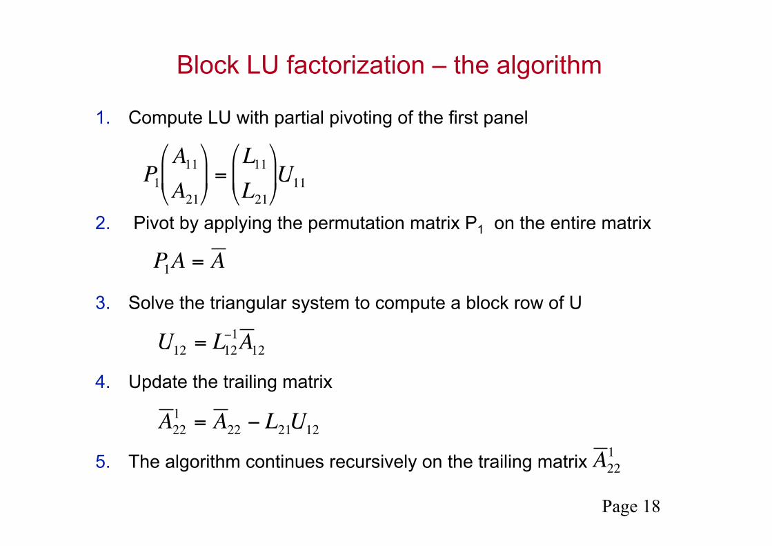
Block LU factorization – the algorithm

1.  Compute LU with partial pivoting of the first panel

2.  Pivot by applying the permutation matrix P1 on the entire matrix

3.  Solve the triangular system to compute a block row of U

4.  Update the trailing matrix

5.  The algorithm continues recursively on the trailing matrix

€

P1A11A21

⎛

⎝ ⎜

⎞

⎠ ⎟ =

L11L21

⎛

⎝ ⎜

⎞

⎠ ⎟ U11

€

P1A = A

€

U12 = L12−1A 12

€

A 221 = A 22 − L21U12

€

A 221

LU factorization (as in ScaLAPACK pdgetrf) LU factorization on a P = Pr x Pc grid of processors For ib = 1 to n-1 step b A(ib) = A(ib:n, ib:n)

(1) Compute panel factorization - find pivot in each column, swap rows

(2) Apply all row permutations - broadcast pivot information along the rows - swap rows at left and right

(3) Compute block row of U - broadcast right diagonal block of L of current panel

(4) Update trailing matrix - broadcast right block column of L - broadcast down block row of U

L

U

A(ib)

L

U

A(ib+b)

L

U

A(ib)

L

U

A(ib)

)log( 2 rPnO

)log/( 2 cPbnO

))log(log/( 22 rc PPbnO +


#messages

General scheme for QR factorization by Householder transformations

The Householder matrix

has the following properties: •  is symmetric and orthogonal, Hi

2 = I, •  is independent of the scaling of hi, •  it reflects x about the hyperplane

•  For QR, we choose a Householder matrix that allows to annihilate the elements of a vector x, except first one.

€

Hi = I −τ ihihiT

€

span(hi)⊥

€

hi

€

x

€

span(hi)⊥

General scheme for QR factorization by Householder transformations

•  Apply Householder transformations to annihilate subdiagonal entries

•  For A of size mxn, the factorization can be written as:

€

A =

x x x xx x x xx x x xx x x x

⎛

⎝

⎜ ⎜ ⎜ ⎜

⎞

⎠

⎟ ⎟ ⎟ ⎟

= H1

x x x x0 x x x0 x x x0 x x x

⎛

⎝

⎜ ⎜ ⎜ ⎜

⎞

⎠

⎟ ⎟ ⎟ ⎟

= H1

1˜ H 2

⎛

⎝ ⎜

⎞

⎠ ⎟

x x x x0 x x x0 0 x x0 0 x x

⎛

⎝

⎜ ⎜ ⎜ ⎜

⎞

⎠

⎟ ⎟ ⎟ ⎟

=

= H1H2

11

˜ H 3

⎛

⎝

⎜ ⎜ ⎜

⎞

⎠

⎟ ⎟ ⎟

x x x x0 x x x0 0 x x0 0 0 x

⎛

⎝

⎜ ⎜ ⎜ ⎜

⎞

⎠

⎟ ⎟ ⎟ ⎟

= H1H2H3R = QR

Compact representation for Q

•  Orthogonal factor Q can be represented implicitly as

•  Example for b=2:

€

Q = H1H2KHb = (I −τ1h1h1T )K(I −τbhbhb

T ) = I −YTYT , where

Y = h1 h2 K hb( )

€

Y = (h1 h2), T =τ1 -τ1h1

T h2τ2

τ2

⎛

⎝ ⎜

⎞

⎠ ⎟

T Y YT I

Algebra of block QR factorization

Matrix A of size nxn is partitioned as

Block QR algebra

The first step of the block QR factorization algorithm computes:

The algorithm continues recursively on the trailing matrix A221

€

A =A11 A12

A21 A22

⎡

⎣ ⎢

⎤

⎦ ⎥ , where A11 is b × b

€

Q1T A =

R11 R12A221

⎡

⎣ ⎢

⎤

⎦ ⎥

Block QR factorization

Block QR algebra: 1.  Compute panel factorization:

2.  Compute the compact representation:

3.  Update the trailing matrix:

4.  The algorithm continues recursively on the trailing matrix.

€

A =A11 A12A21 A22

⎛

⎝ ⎜

⎞

⎠ ⎟ =Q1

R11 R12A22

1

⎛

⎝ ⎜

⎞

⎠ ⎟

€

A11

A12

⎛

⎝ ⎜

⎞

⎠ ⎟ = Q1

R11⎛

⎝ ⎜

⎞

⎠ ⎟ , Q1 = H1H2...Hb

€

Q1 = I −Y1T1Y1T

€

I −Y1T1TY1

T( ) A12A22⎛

⎝ ⎜

⎞

⎠ ⎟ =

A12A22

⎛

⎝ ⎜

⎞

⎠ ⎟ −Y1 T1

T Y1T A12A22

⎛

⎝ ⎜

⎞

⎠ ⎟

⎛

⎝ ⎜ ⎜

⎞

⎠ ⎟ ⎟

⎛

⎝ ⎜ ⎜

⎞

⎠ ⎟ ⎟ =

R12A221

⎛

⎝ ⎜

⎞

⎠ ⎟

T1 Y1 Y1T I

TSQR: QR factorization of a tall skinny matrix using Householder transformations

W =

W0 W1 W2 W3

R00 R10 R20 R30

R01

R11

R02

•  QR decomposition of m x b matrix W, m >> b •  P processors, block row layout

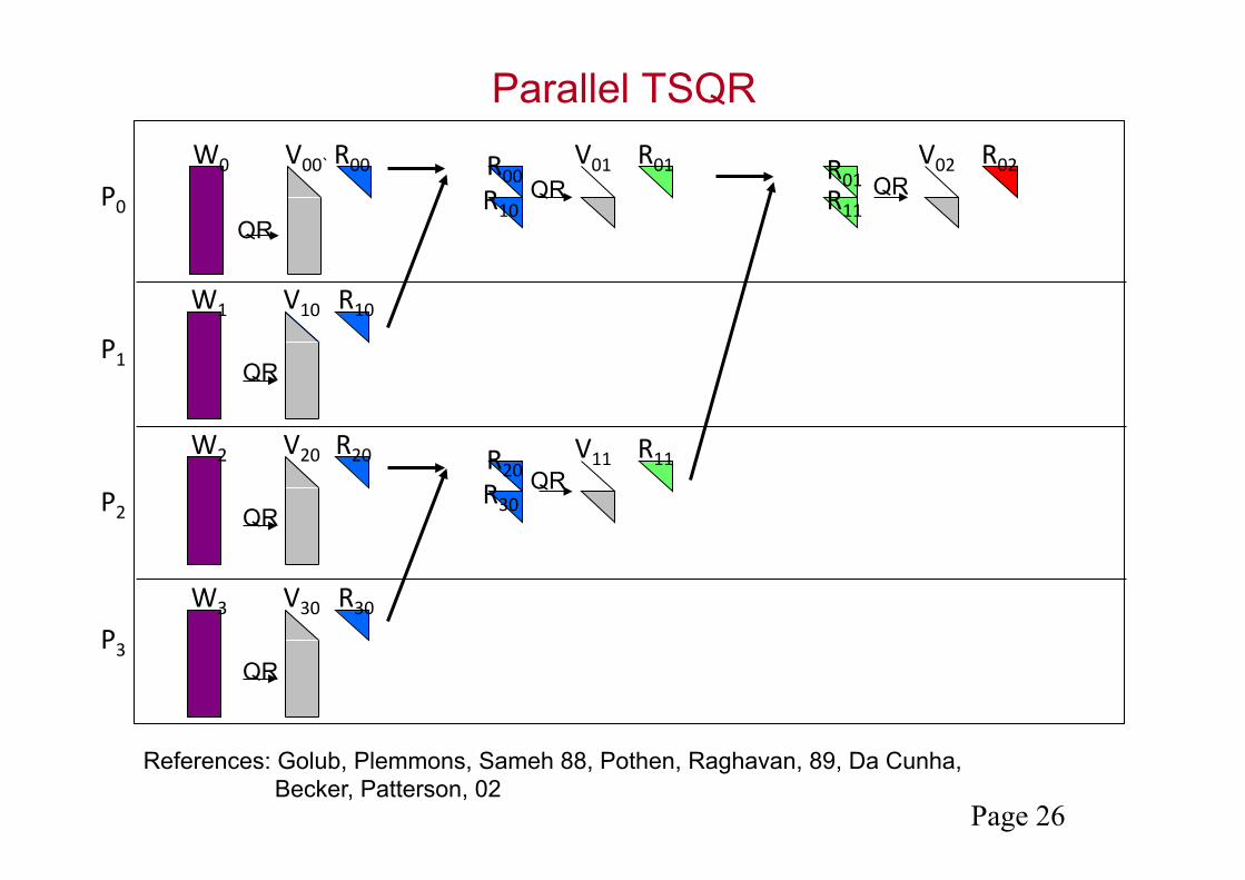
•  Classic Parallel Algorithm •  Compute Householder vector for each column •  Number of messages ∝ b log P

•  Communication Avoiding Algorithm •  Reduction operation, with QR as operator •  Number of messages ∝ log P

J. Demmel, LG, M. Hoemmen, J. Langou, 08

Parallel TSQR

QR

R00 V00` W0

R10 V10 W1

R20 V20 W2

R30 V30 W3

R00

R10 V01

R01

R20

R30 V11

R11

P0

P1

P2

P3

V02 R02 R01

R11

QR

QR

QR

QR

QR

QR

References: Golub, Plemmons, Sameh 88, Pothen, Raghavan, 89, Da Cunha, Becker, Patterson, 02

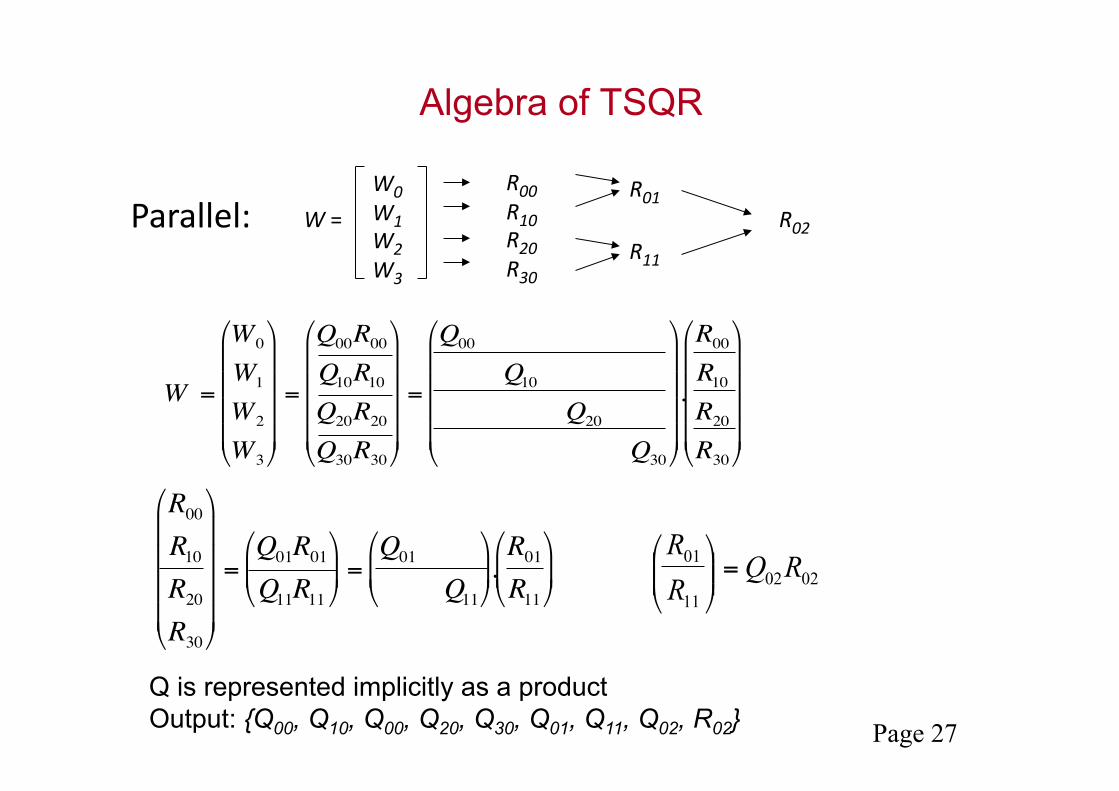
Q is represented implicitly as a product Output: {Q00, Q10, Q00, Q20, Q30, Q01, Q11, Q02, R02}

€

W =

W0

W1

W2

W3

⎛

⎝

⎜ ⎜ ⎜ ⎜

⎞

⎠

⎟ ⎟ ⎟ ⎟

=

Q00R00Q10R10Q20R20Q30R30

⎛

⎝

⎜ ⎜ ⎜ ⎜

⎞

⎠

⎟ ⎟ ⎟ ⎟

=

Q00

Q10Q20

Q30

⎛

⎝

⎜ ⎜ ⎜ ⎜

⎞

⎠

⎟ ⎟ ⎟ ⎟

.

R00R10R20R30

⎛

⎝

⎜ ⎜ ⎜ ⎜

⎞

⎠

⎟ ⎟ ⎟ ⎟

€

R00R10R20R30

⎛

⎝

⎜ ⎜ ⎜ ⎜

⎞

⎠

⎟ ⎟ ⎟ ⎟

=Q01R01Q11R11

⎛

⎝ ⎜

⎞

⎠ ⎟ =

Q01

Q11

⎛

⎝ ⎜

⎞

⎠ ⎟ .R01R11

⎛

⎝ ⎜

⎞

⎠ ⎟ 0202

11

01 RQRR

=⎟⎟⎠

⎞⎜⎜⎝

⎛

Algebra of TSQR

W =

W0 W1 W2 W3

R00 R10 R20 R30

R01

R11

R02 Parallel:

Q is represented implicitly as a product

⎟⎟⎟⎟⎟

⎠

⎞

⎜⎜⎜⎜⎜

⎝

⎛

⎟⎟⎟⎟⎟

⎠

⎞

⎜⎜⎜⎜⎜

⎝

⎛

=

⎟⎟⎟⎟⎟

⎠

⎞

⎜⎜⎜⎜⎜

⎝

⎛

=

30

20

10

00

30

20

10

00

3

2

1

0

.

RRRR

QQ

QQ

WWWW

W

⎟⎟⎠

⎞⎜⎜⎝

⎛⎟⎟⎠

⎞⎜⎜⎝

⎛=

⎟⎟⎟⎟⎟

⎠

⎞

⎜⎜⎜⎜⎜

⎝

⎛

11

01

11

01

30

20

10

00

.RR

QQ

RRRR

020211

01 RQRR

=⎟⎟⎠

⎞⎜⎜⎝

⎛

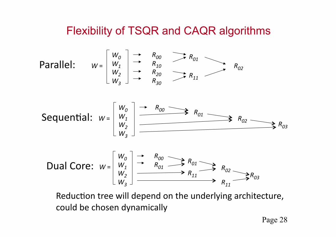
Flexibility of TSQR and CAQR algorithms

W =

W0 W1 W2 W3

R00 R10 R20 R30

R01

R11

R02 Parallel:

W =

W0 W1 W2 W3

R01 R02

R00

R03 Sequen8al:

W =

W0 W1 W2 W3

R00 R01

R01 R11

R02

R11 R03

Dual Core:

Reduc8on tree will depend on the underlying architecture, could be chosen dynamically

Algebra of TSQR

W =

W0 W1 W2 W3

R00 R10 R20 R30

R01

R11

R02 Parallel:

CAQR

QR for General Matrices •  Cost of CAQR vs ScaLAPACK’s PDGEQRF

•  n x n matrix on P1/2 x P1/2 processor grid, block size b •  Flops: (4/3)n3/P + (3/4)n2b log P/P1/2 vs (4/3)n3/P •  Bandwidth: (3/4)n2 log P/P1/2 vs same •  Latency: 2.5 n log P / b vs 1.5 n log P

•  Close to optimal (modulo log P factors) •  Assume: O(n2/P) memory/processor, O(n3) algorithm, •  Choose b near n / P1/2 (its upper bound) •  Bandwidth lower bound: Ω(n2 /P1/2) – just log(P) smaller •  Latency lower bound: Ω(P1/2) – just polylog(P) smaller

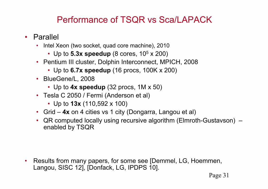
Performance of TSQR vs Sca/LAPACK

•  Parallel •  Intel Xeon (two socket, quad core machine), 2010

•  Up to 5.3x speedup (8 cores, 105 x 200) •  Pentium III cluster, Dolphin Interconnect, MPICH, 2008

•  Up to 6.7x speedup (16 procs, 100K x 200) •  BlueGene/L, 2008

•  Up to 4x speedup (32 procs, 1M x 50) •  Tesla C 2050 / Fermi (Anderson et al)

•  Up to 13x (110,592 x 100) •  Grid – 4x on 4 cities vs 1 city (Dongarra, Langou et al) •  QR computed locally using recursive algorithm (Elmroth-Gustavson) –

enabled by TSQR

•  Results from many papers, for some see [Demmel, LG, Hoemmen, Langou, SISC 12], [Donfack, LG, IPDPS 10].

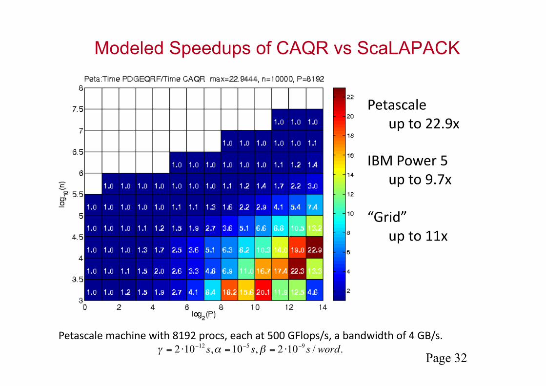
Modeled Speedups of CAQR vs ScaLAPACK

Petascale up to 22.9x

IBM Power 5 up to 9.7x

“Grid” up to 11x

Petascale machine with 8192 procs, each at 500 GFlops/s, a bandwidth of 4 GB/s. ./102,10,102 9512 wordsss −−− ⋅==⋅= βαγ

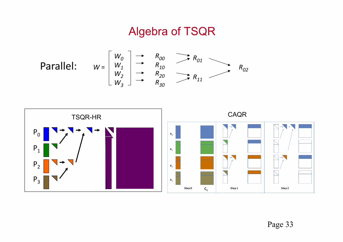
Algebra of TSQR

W =

W0 W1 W2 W3

R00 R10 R20 R30

R01

R11

R02 Parallel:

P0

P1

P2

P3

TSQR-HR CAQR

Reconstruct Householder vectors from TSQR

The QR factorization using Householder vectors

can be re-written as an LU factorization

€

W =QR = (I −YTY1T )R

€

W − R =Y (−TY1T )R

Q − I =Y (−TY1T )

I Q -‐ T Y Y1T

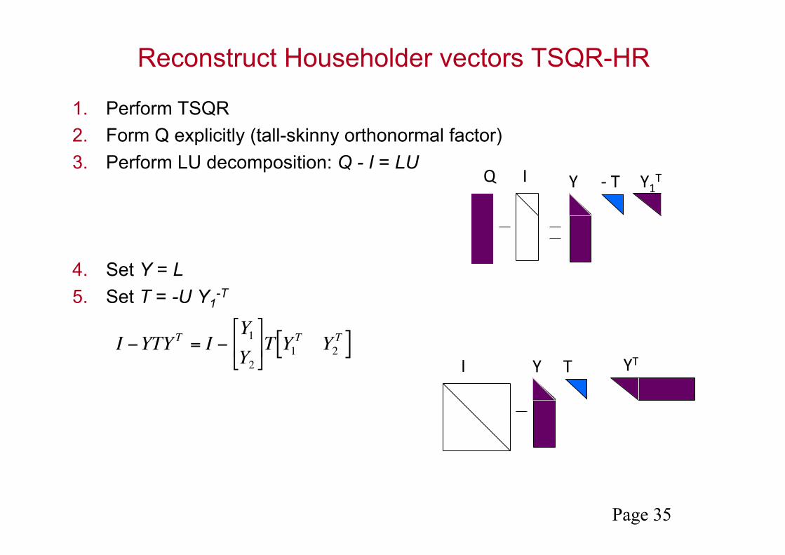
Reconstruct Householder vectors TSQR-HR

1.  Perform TSQR 2.  Form Q explicitly (tall-skinny orthonormal factor) 3.  Perform LU decomposition: Q - I = LU

4.  Set Y = L 5.  Set T = -U Y1

-T

€

I −YTYT = I −Y1Y2

⎡

⎣ ⎢

⎤

⎦ ⎥ T Y1

T Y2T[ ]

T Y YT I

I Q -‐ T Y Y1T

Strong scaling

•  Hopper: Cray XE6 (NERSC) – 2 x 12-core AMD Magny-Cours (2.1 GHz) •  Edison: Cray CX30 (NERSC) – 2 x 12-core Intel Ivy Bridge (2.4 GHz) •  Effective flop rate, computed by dividing 2mn2 − 2n3/3 by measured runtime Ballard, Demmel, LG, Jacquelin, Knight, Nguyen, and Solomonik, 2015.

1x

7x

6x

1x

3.7x2.7x

Weak scaling QR on Hopper

•  Matrix of size 15K-by-15K to 131K-by-131K •  Hopper: Cray XE6 supercomputer (NERSC) – dual socket 12-

core Magny-Cours Opteron (2.1 GHz)

The LU factorization of a tall skinny matrix

First try the obvious generalization of TSQR.

⎟⎟⎟⎟⎟

⎠

⎞

⎜⎜⎜⎜⎜

⎝

⎛

⋅

⎟⎟⎟⎟⎟

⎠

⎞

⎜⎜⎜⎜⎜

⎝

⎛

⎟⎟⎟⎟⎟

⎠

⎞

⎜⎜⎜⎜⎜

⎝

⎛

∏

∏

∏

∏

=

⎟⎟⎟⎟⎟

⎠

⎞

⎜⎜⎜⎜⎜

⎝

⎛

=

Π

30

20

10

00

30

20

10

00

30

20

10

00

3

2

1

0

.

0

UUUU

LL

LL

WWWW

W

4444 34444 21

⎟⎟⎠

⎞⎜⎜⎝

⎛⎟⎟⎠

⎞⎜⎜⎝

⎛⎟⎟⎠

⎞⎜⎜⎝

⎛

∏

∏=

⎟⎟⎟⎟⎟

⎠

⎞

⎜⎜⎜⎜⎜

⎝

⎛

Π

11

01

11

01

11

01

30

20

10

00

..

1

UU

LL

UUUU

43421{ 020202

11

01

2

ULUU

∏

∏=⎟⎟⎠

⎞⎜⎜⎝

⎛

Obvious generalization of TSQR to LU

•  Block parallel pivoting: •  uses a binary tree and is optimal in the parallel case

•  Block pairwise pivoting: •  uses a flat tree and is optimal in the sequential case •  introduced by Barron and Swinnerton-Dyer, 1960: block LU factorization used to solve a

system with 100 equations on EDSAC 2 computer using an auxiliary magnetic-tape •  used in PLASMA for multicore architectures and FLAME for out-of-core algorithms and

for multicore architectures

W =

W0 W1 W2 W3

U00 U10 U20 U30

U01

U11

U02

W=

W0 W1 W2 W3

U01 U02

U00

U03

Stability of the LU factorization •  The backward stability of the LU factorization of a matrix A of size n-by-n

depends on the growth factor

where aijk are the values at the k-th step.

•  gW ≤ 2n-1 , attained for Wilkinson matrix

but in practice it is on the order of n2/3 -- n1/2

•  Two reasons considered to be important for the average case stability [Trefethen and Schreiber, 90] :

- the multipliers in L are small,

- the correction introduced at each elimination step is of rank 1.

€

gW =maxi, j ,k aij

k

maxi, j aij

€

ˆ L ⋅ ˆ U ∞≤ (1+ 2(n2 − n)gw ) A ∞

€

A = diag(±1)

1 0 0 L 0 1−1 1 L 0 1−1 −1 1 O 0 1M M O O M M

−1 −1 L −1 1 1−1 −1 L −1 −1 1

⎛

⎝

⎜ ⎜ ⎜ ⎜ ⎜ ⎜ ⎜

⎞

⎠

⎟ ⎟ ⎟ ⎟ ⎟ ⎟ ⎟

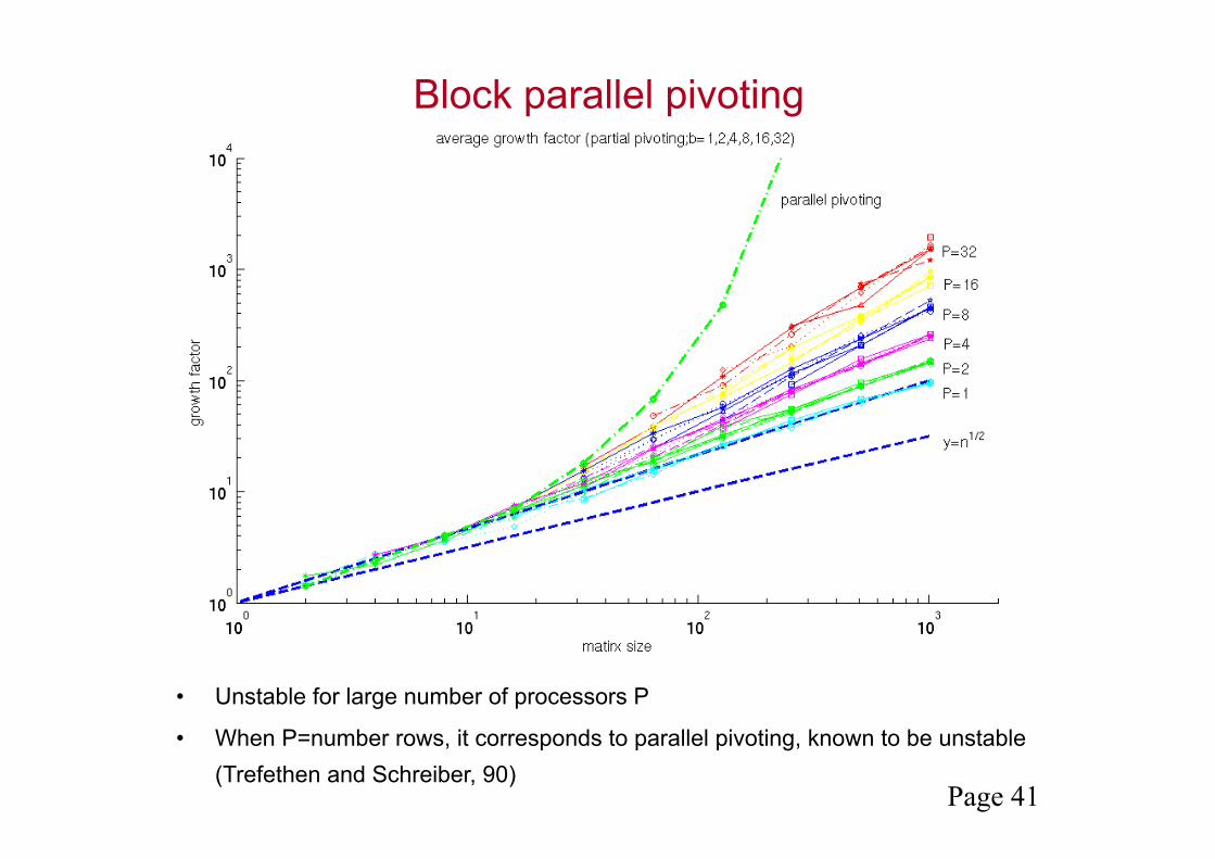
Block parallel pivoting

•  Unstable for large number of processors P

•  When P=number rows, it corresponds to parallel pivoting, known to be unstable (Trefethen and Schreiber, 90)

Block pairwise pivoting

•  Results shown for random matrices •  Will become unstable for large matrices W=

W0 W1 W2 W3

U01 U02

U00

U03

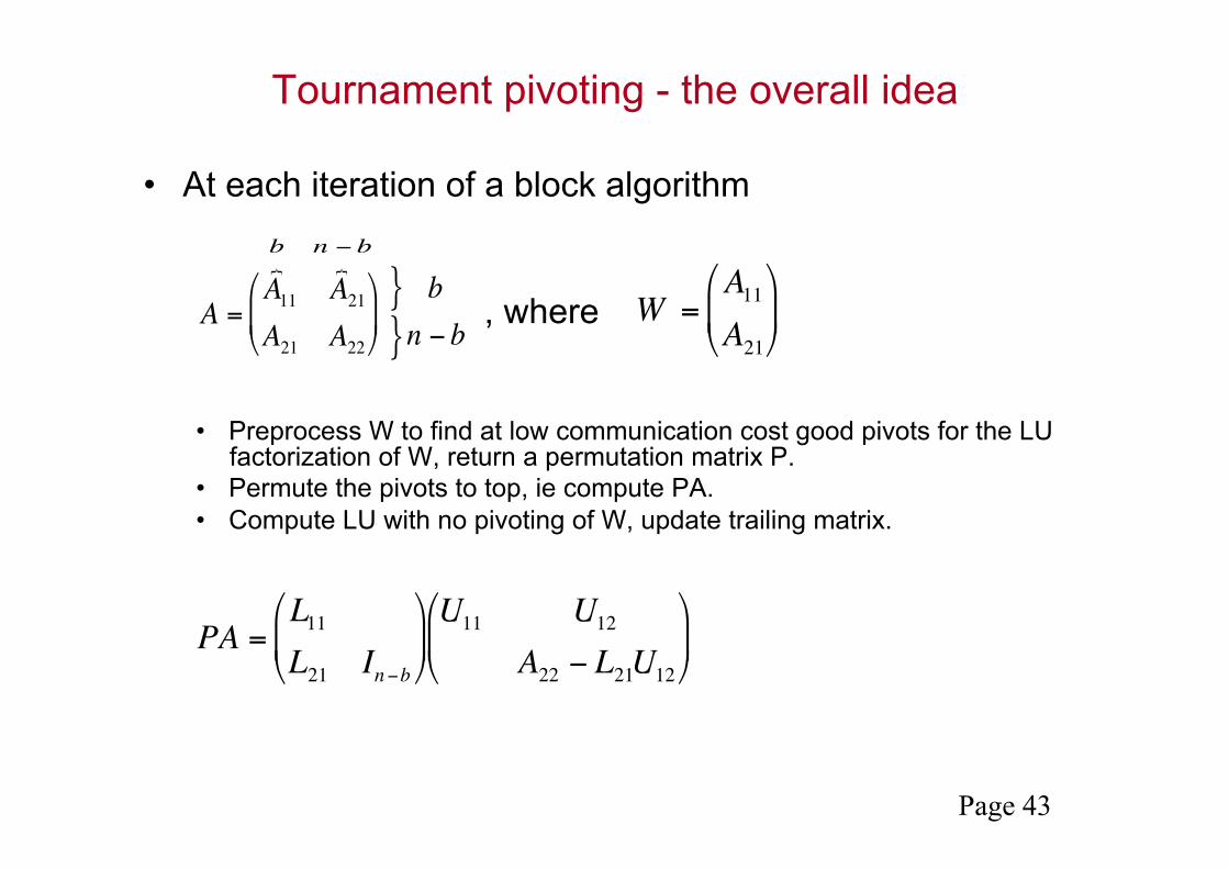
Tournament pivoting - the overall idea

•  At each iteration of a block algorithm

, where

•  Preprocess W to find at low communication cost good pivots for the LU factorization of W, return a permutation matrix P.

•  Permute the pivots to top, ie compute PA. •  Compute LU with no pivoting of W, update trailing matrix.

€

W =A11A21

⎛

⎝ ⎜

⎞

⎠ ⎟

€

A =A11 A21A21 A22

⎛

⎝ ⎜

⎞

⎠ ⎟

€

}}

bn − b

€

b n − b} }

€

PA =L11L21 In−b

⎛

⎝ ⎜

⎞

⎠ ⎟ U11 U12

A22 − L21U12

⎛

⎝ ⎜

⎞

⎠ ⎟

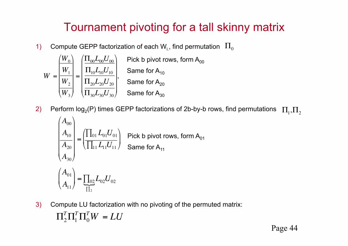
Tournament pivoting for a tall skinny matrix 1)  Compute GEPP factorization of each Wi., find permutation

2)  Perform log2(P) times GEPP factorizations of 2b-by-b rows, find permutations

3)  Compute LU factorization with no pivoting of the permuted matrix:

€

W =

W0

W1

W2

W3

⎛

⎝

⎜ ⎜ ⎜ ⎜

⎞

⎠

⎟ ⎟ ⎟ ⎟

=

Π00L00U00

Π10L10U10

Π20L20U20

Π30L30U30

⎛

⎝

⎜ ⎜ ⎜ ⎜

⎞

⎠

⎟ ⎟ ⎟ ⎟

,

€

A00A10A20A30

⎛

⎝

⎜ ⎜ ⎜ ⎜

⎞

⎠

⎟ ⎟ ⎟ ⎟

=∏01L01U01

∏11L11U11

⎛

⎝ ⎜

⎞

⎠ ⎟

€

A01A11

⎛

⎝ ⎜

⎞

⎠ ⎟ =∏02

∏2

{L02U02

€

Π2TΠ1

TΠ0TW = LU

Pick b pivot rows, form A00

Same for A10

Same for A20

Same for A30

Pick b pivot rows, form A01

Same for A11

€

Π0

€

Π1,Π2

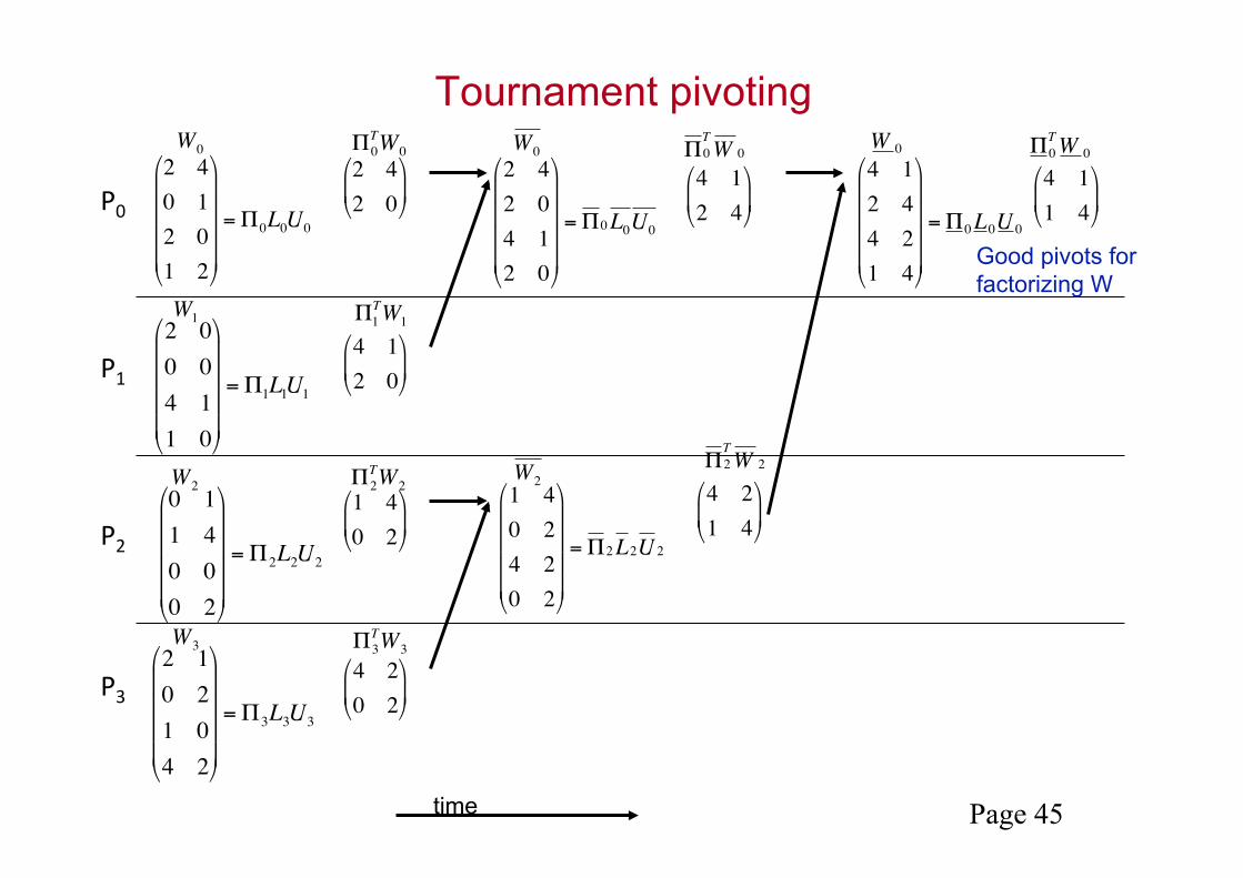
Tournament pivoting

time

P0

P1

P2

P3

€

2 40 12 01 2

⎛

⎝

⎜ ⎜ ⎜ ⎜

⎞

⎠

⎟ ⎟ ⎟ ⎟

=Π0L0U0

€

2 00 04 11 0

⎛

⎝

⎜ ⎜ ⎜ ⎜

⎞

⎠

⎟ ⎟ ⎟ ⎟

=Π1L1U1

€

0 11 40 00 2

⎛

⎝

⎜ ⎜ ⎜ ⎜

⎞

⎠

⎟ ⎟ ⎟ ⎟

=Π2L2U2

€

2 10 21 04 2

⎛

⎝

⎜ ⎜ ⎜ ⎜

⎞

⎠

⎟ ⎟ ⎟ ⎟

=Π3L3U3

€

2 42 0⎛

⎝ ⎜

⎞

⎠ ⎟

€

4 12 0⎛

⎝ ⎜

⎞

⎠ ⎟

€

1 40 2⎛

⎝ ⎜

⎞

⎠ ⎟

€

4 20 2⎛

⎝ ⎜

⎞

⎠ ⎟

€

2 42 04 12 0

⎛

⎝

⎜ ⎜ ⎜ ⎜

⎞

⎠

⎟ ⎟ ⎟ ⎟

=Π0L0U0

€

1 40 24 20 2

⎛

⎝

⎜ ⎜ ⎜ ⎜

⎞

⎠

⎟ ⎟ ⎟ ⎟

=Π2L2U 2

€

4 12 4⎛

⎝ ⎜

⎞

⎠ ⎟

€

4 21 4⎛

⎝ ⎜

⎞

⎠ ⎟

€

4 12 44 21 4

⎛

⎝

⎜ ⎜ ⎜ ⎜

⎞

⎠

⎟ ⎟ ⎟ ⎟

=Π0L0U 0

€

4 11 4⎛

⎝ ⎜

⎞

⎠ ⎟

€

W0

€

Π0TW0

€

W0

€

Π0TW 0

€

W 0

€

Π0TW 0

€

W1

€

Π1TW1

€

W2

€

Π2TW2

€

W2

€

Π2TW 2

€

W3

€

Π3TW3

Good pivots for factorizing W

Growth factor for binary tree based CALU

•  Random matrices from a normal distribution •  Same behaviour for all matrices in our test, and |L| <= 4.2

Stability of CALU (experimental results)

Summer School Lecture 4 47

•  Results show ||PA-LU||/||A||, normwise and componentwise backward errors, for random matrices and special ones

•  See [LG, Demmel, Xiang, SIMAX 2011] for details •  BCALU denotes binary tree based CALU and FCALU denotes flat tree based CALU

Our “proof of stability” for CALU •  CALU as stable as GEPP in following sense: In exact arithmetic, CALU process on a matrix A is equivalent to GEPP

process on a larger matrix G whose entries are blocks of A and zeros.

•  Example of one step of tournament pivoting:

•  Proof possible by using original rows of A during tournament pivoting (not the computed rows of U).

€

A =

A11 A12A21 A22A31 A32

⎛

⎝

⎜ ⎜ ⎜

⎞

⎠

⎟ ⎟ ⎟

€

G =

A11 A12A21 A21

−A31 A32

⎛

⎝

⎜ ⎜ ⎜

⎞

⎠

⎟ ⎟ ⎟

A11 A21 A31

A11

A21 A11

tournament pivoting:

LU factorization and low rank matrices •  For low rank matrices, the factorization of A1 computed as following might not

be stable Compute PA=LU by using GEPP L(k+1:end,k) = A(k+1:end,k)/A(k,k) Permute the matrix A1=PA Compute LU with no pivoting A1=L1U1 L(k+1:end,k) = L(k+1:end,k)* (1/A(k,k))

•  Example A = randn(6,3)*randn(3,5), max(abs(L)) = 1, max(abs(L1)) = 1015

€

After 4 steps of factorization of A1 we obtain :

A14 =

1.00000.1729 1.00000.6061 0.8608 1.00000.5776 0.0543 0.3264 1.00000.4789 −0.2877 −0.1545 2.3333 4.9e − 32−0.3264 −0.7514 −0.4597 1.7778 −7.4e −17

⎛

⎝

⎜ ⎜ ⎜ ⎜ ⎜ ⎜ ⎜

⎞

⎠

⎟ ⎟ ⎟ ⎟ ⎟ ⎟ ⎟

⋅

4.4766 3.0163 −4.7390 4.2180 −0.8164−1.5439 −0.4703 1.9267 1.0925

1.6149 2.3623 0.31679.9e −16 1.6e −16

1

⎛

⎝

⎜ ⎜ ⎜ ⎜ ⎜ ⎜

⎞

⎠

⎟ ⎟ ⎟ ⎟ ⎟ ⎟

€

After 4 steps of factorization of PA we obtain :

PA4 =

1.00000.1729 1.00000.6061 0.8608 1.00000.5776 0.0543 0.3264 1.00000.4789 −0.2877 −0.1545 2.3333 2.3e −16−0.3264 −0.7514 −0.4597 1.7778 8.3e −17

⎛

⎝

⎜ ⎜ ⎜ ⎜ ⎜ ⎜ ⎜

⎞

⎠

⎟ ⎟ ⎟ ⎟ ⎟ ⎟ ⎟

⋅

4.4766 3.0163 −4.7390 4.2180 −0.8164−1.5439 −0.4703 1.9267 1.0925

1.6149 2.3623 0.31679.9e −16 1.6e −16

1

⎛

⎝

⎜ ⎜ ⎜ ⎜ ⎜ ⎜

⎞

⎠

⎟ ⎟ ⎟ ⎟ ⎟ ⎟

Schur complement after 4 elimination steps

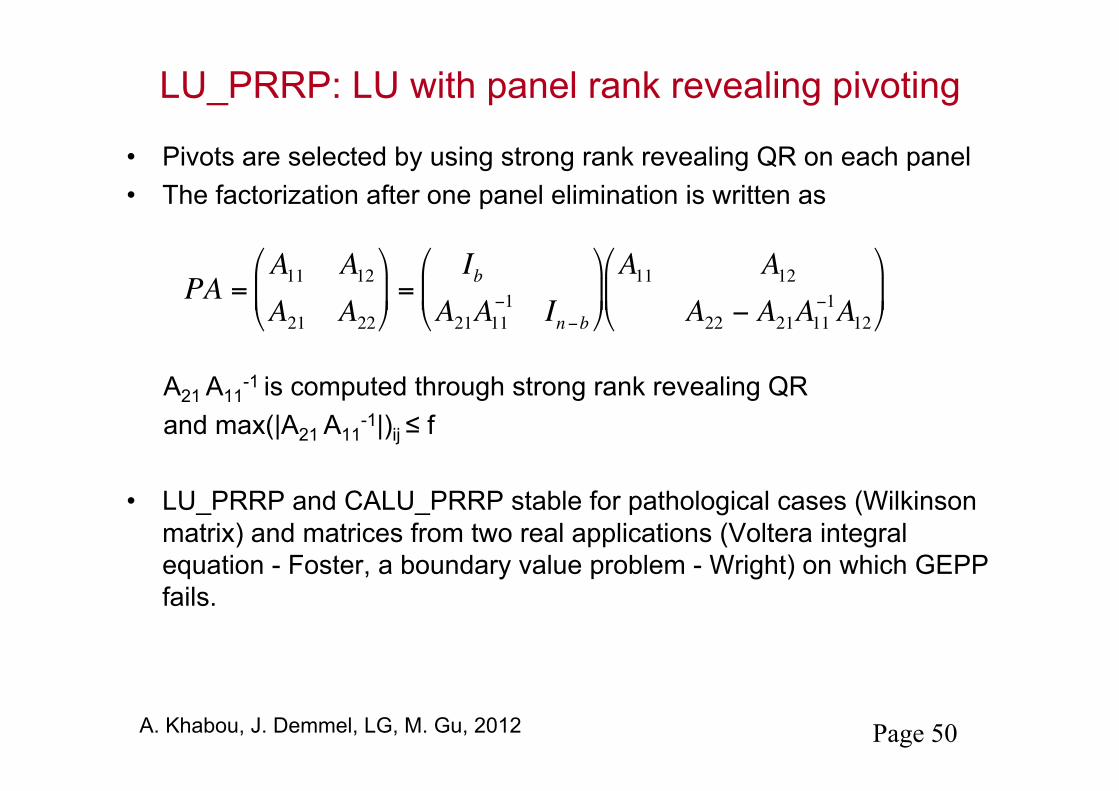
LU_PRRP: LU with panel rank revealing pivoting

•  Pivots are selected by using strong rank revealing QR on each panel •  The factorization after one panel elimination is written as

A21 A11-1 is computed through strong rank revealing QR

and max(|A21 A11-1|)ij ≤ f

•  LU_PRRP and CALU_PRRP stable for pathological cases (Wilkinson matrix) and matrices from two real applications (Voltera integral equation - Foster, a boundary value problem - Wright) on which GEPP fails.

A. Khabou, J. Demmel, LG, M. Gu, 2012

€

PA =A11 A12A21 A22

⎛

⎝ ⎜

⎞

⎠ ⎟ =

IbA21A11

−1 In−b

⎛

⎝ ⎜

⎞

⎠ ⎟ A11 A12

A22 − A21A11−1A12

⎛

⎝ ⎜

⎞

⎠ ⎟

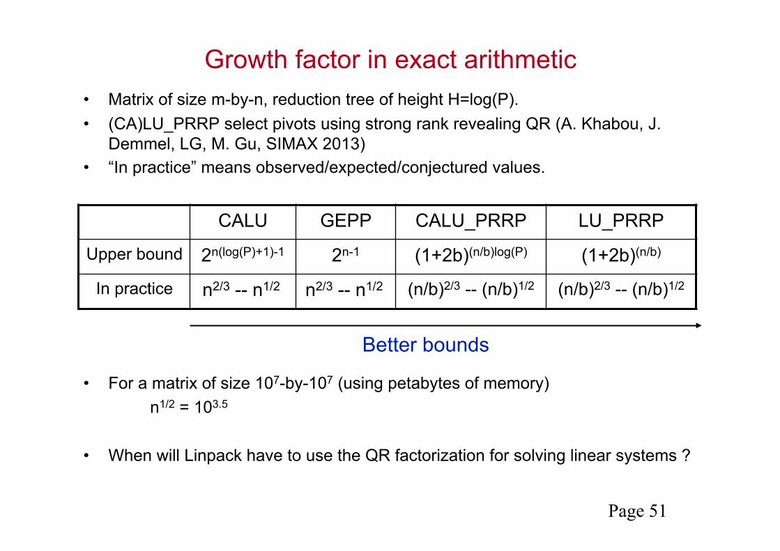
Growth factor in exact arithmetic •  Matrix of size m-by-n, reduction tree of height H=log(P). •  (CA)LU_PRRP select pivots using strong rank revealing QR (A. Khabou, J.

Demmel, LG, M. Gu, SIMAX 2013) •  “In practice” means observed/expected/conjectured values.

•  For a matrix of size 107-by-107 (using petabytes of memory) n1/2 = 103.5

•  When will Linpack have to use the QR factorization for solving linear systems ?

Better bounds

CALU GEPP CALU_PRRP LU_PRRP

Upper bound 2n(log(P)+1)-1 2n-1 (1+2b)(n/b)log(P) (1+2b)(n/b)

In practice n2/3 -- n1/2 n2/3 -- n1/2 (n/b)2/3 -- (n/b)1/2 (n/b)2/3 -- (n/b)1/2

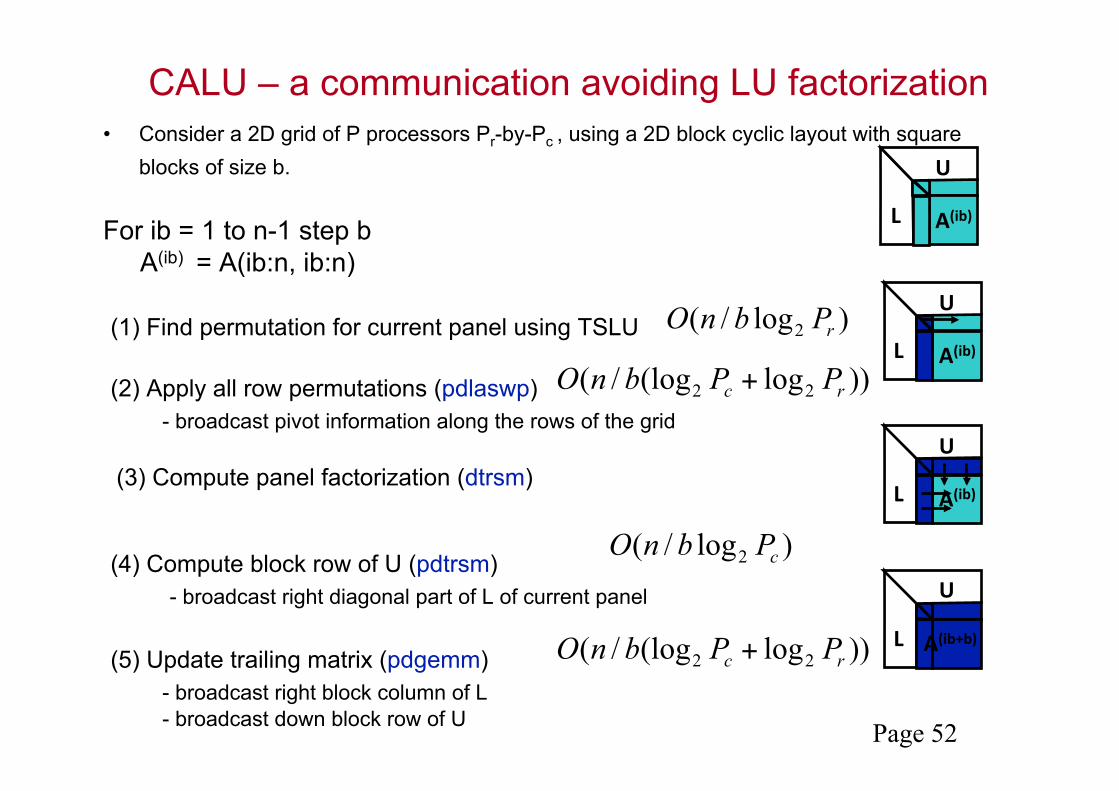
CALU – a communication avoiding LU factorization •  Consider a 2D grid of P processors Pr-by-Pc , using a 2D block cyclic layout with square

blocks of size b.

For ib = 1 to n-1 step b A(ib) = A(ib:n, ib:n)

(1) Find permutation for current panel using TSLU

(2) Apply all row permutations (pdlaswp) - broadcast pivot information along the rows of the grid

(3) Compute panel factorization (dtrsm)

(4) Compute block row of U (pdtrsm) - broadcast right diagonal part of L of current panel

(5) Update trailing matrix (pdgemm) - broadcast right block column of L - broadcast down block row of U

L

U

A(ib)

L

U

A(ib+b)

L

U

A(ib)

L

U

A(ib)

)log/( 2 rPbnO

)log/( 2 cPbnO



LU for General Matrices

•  Cost of CALU vs ScaLAPACK’s PDGETRF •  n x n matrix on P1/2 x P1/2 processor grid, block size b •  Flops: (2/3)n3/P + (3/2)n2b / P1/2 vs (2/3)n3/P + n2b/P1/2 •  Bandwidth: n2 log P/P1/2 vs same •  Latency: 3 n log P / b vs 1.5 n log P+ 3.5n logP / b

•  Close to optimal (modulo log P factors) •  Assume: O(n2/P) memory/processor, O(n3) algorithm, •  Choose b near n / P1/2 (its upper bound) •  Bandwidth lower bound: Ω(n2 /P1/2) – just log(P) smaller •  Latency lower bound: Ω(P1/2) – just polylog(P) smaller

Performance vs ScaLAPACK

•  Parallel TSLU (LU on tall-skinny matrix) •  IBM Power 5

•  Up to 4.37x faster (16 procs, 1M x 150) •  Cray XT4

•  Up to 5.52x faster (8 procs, 1M x 150)

•  Parallel CALU (LU on general matrices) •  Intel Xeon (two socket, quad core)

•  Up to 2.3x faster (8 cores, 10^6 x 500) •  IBM Power 5

•  Up to 2.29x faster (64 procs, 1000 x 1000) •  Cray XT4

•  Up to 1.81x faster (64 procs, 1000 x 1000)

•  Details in SC08 (LG, Demmel, Xiang), IPDPS’10 (S. Donfack, LG).

CALU and its task dependency graph

•  The matrix is partitioned into blocks of size T x b. •  The computation of each block is associated with a task.

Scheduling CALU’s Task Dependency Graph •  Static scheduling

+ Good locality of data - Ignores noise

•  Dynamic scheduling + Keeps cores busy - Poor usage of data locality - Can have large dequeue overhead

Lightweight scheduling

•  Emerging complexities of multi- and mani-core processors suggest a need for self-adaptive strategies •  One example is work stealing

•  Goal: •  Design a tunable strategy that is able to provide a good trade-off between load

balance, data locality, and dequeue overhead. •  Provide performance consistency

•  Approach: combine static and dynamic scheduling •  Shown to be efficient for regular mesh computation [B. Gropp and V. Kale]

Data layout/scheduling Static Dynamic Static/(%dynamic)

Column Major Layout (CM) √

Block Cyclic Layout (BCL) √ √ √

2-level Block Layout (2l-BL) √ √ √

Design space

S. Donfack, LG, B. Gropp, V. Kale,IPDPS 2012

Lightweight scheduling

•  A self-adaptive strategy to provide •  A good trade-off between load balance, data locality, and dequeue overhead. •  Performance consistency •  Shown to be efficient for regular mesh computation [B. Gropp and V. Kale]

S. Donfack, LG, B. Gropp, V. Kale, 2012

Combined static/dynamic scheduling: •  A thread executes in priority its

statically assigned tasks •  When no task ready, it picks a

ready task from the dynamic part •  The size of the dynamic part is

guided by a performance model

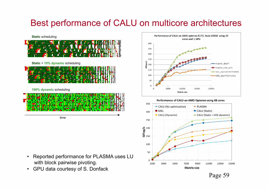
Best performance of CALU on multicore architectures

•  Reported performance for PLASMA uses LU with block pairwise pivoting. •  GPU data courtesy of S. Donfack

Static scheduling

time

Static + 10% dynamic scheduling

100% dynamic scheduling

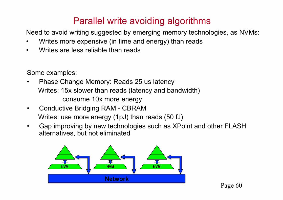
Parallel write avoiding algorithms Need to avoid writing suggested by emerging memory technologies, as NVMs: •  Writes more expensive (in time and energy) than reads •  Writes are less reliable than reads

Some examples: •  Phase Change Memory: Reads 25 us latency Writes: 15x slower than reads (latency and bandwidth) consume 10x more energy •  Conductive Bridging RAM - CBRAM Writes: use more energy (1pJ) than reads (50 fJ) •  Gap improving by new technologies such as XPoint and other FLASH

alternatives, but not eliminated

Parallel write-avoiding algorithms

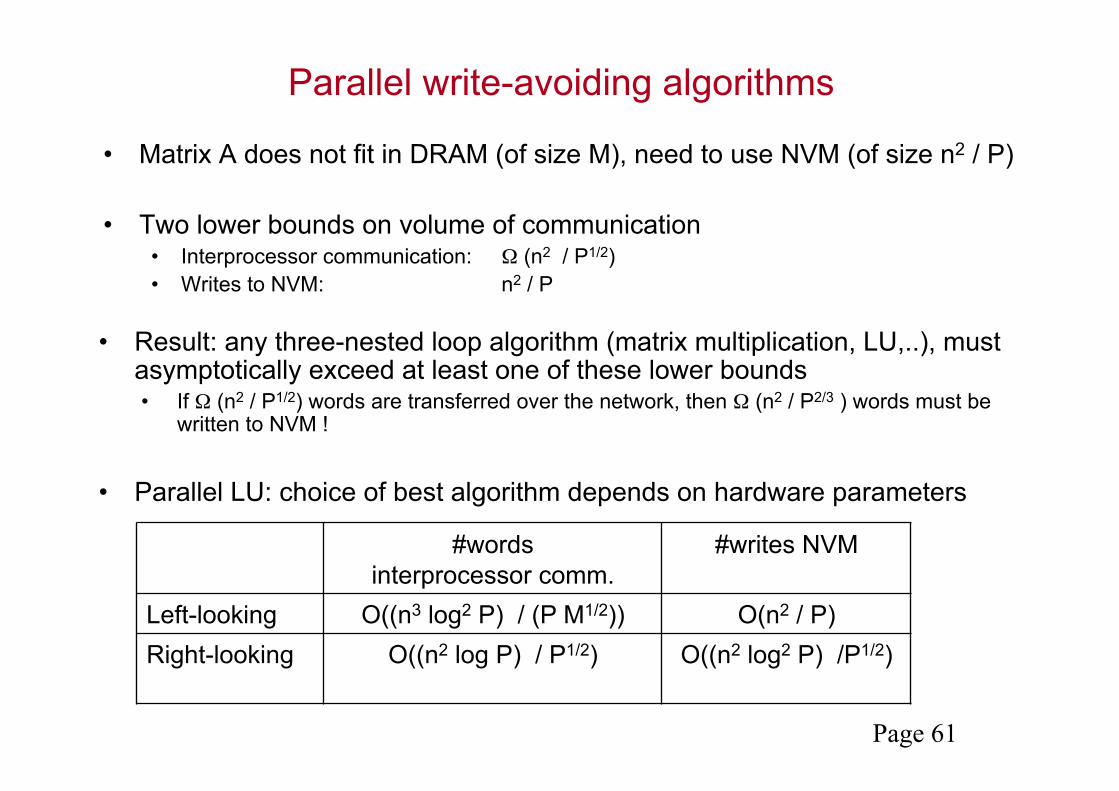
•  Matrix A does not fit in DRAM (of size M), need to use NVM (of size n2 / P)

•  Two lower bounds on volume of communication •  Interprocessor communication: Ω (n2 / P1/2) •  Writes to NVM: n2 / P

#words interprocessor comm.

#writes NVM

Left-looking O((n3 log2 P) / (P M1/2)) O(n2 / P) Right-looking O((n2 log P) / P1/2) O((n2 log2 P) /P1/2)

•  Result: any three-nested loop algorithm (matrix multiplication, LU,..), must asymptotically exceed at least one of these lower bounds •  If Ω (n2 / P1/2) words are transferred over the network, then Ω (n2 / P2/3 ) words must be

written to NVM !

•  Parallel LU: choice of best algorithm depends on hardware parameters

Conclusions

•  Many previous results •  Only several cited, many references given in the papers •  Flat trees algorithms for QR factorization, called tiled algorithms used in the context of

•  Out of core - Gunter, van de Geijn 2005 •  Multicore, Cell processors - Buttari, Langou, Kurzak and Dongarra (2007, 2008),

Quintana-Orti, Quintana-Orti, Chan, van Zee, van de Geijn (2007, 2008)

References

Results presented from: •  J. Demmel, L. Grigori, M. F. Hoemmen, and J. Langou, Communication-optimal parallel and sequential

QR and LU factorizations, UCB-EECS-2008-89, 2008, SIAM journal on Scientific Computing, Vol. 34, No 1, 2012.

•  L. Grigori, J. Demmel, and H. Xiang, Communication avoiding Gaussian elimination, Proceedings of the IEEE/ACM SuperComputing SC08 Conference, November 2008.

•  L. Grigori, J. Demmel, and H. Xiang, CALU: a communication optimal LU factorization algorithm, SIAM. J. Matrix Anal. & Appl., 32, pp. 1317-1350, 2011.

•  M. Hoemmen’s Phd thesis, Communication avoiding Krylov subspace methods, 2010. •  L. Grigori, P.-Y. David, J. Demmel, and S. Peyronnet, Brief announcement: Lower bounds on

communication for sparse Cholesky factorization of a model problem, ACM SPAA 2010. •  S. Donfack, L. Grigori, and A. Kumar Gupta, Adapting communication-avoiding LU and QR

factorizations to multicore architectures, Proceedings of IEEE International Parallel & Distributed Processing Symposium IPDPS, April 2010.

•  S. Donfack, L. Grigori, W. Gropp, and V. Kale, Hybrid static/dynamic scheduling for already optimized dense matrix factorization , Proceedings of IEEE International Parallel & Distributed Processing Symposium IPDPS, 2012.

•  A. Khabou, J. Demmel, L. Grigori, and M. Gu, LU factorization with panel rank revealing pivoting and its communication avoiding version, LAWN 263, SIAM Journal on Matrix Analysis, in revision, 2012.

•  L. Grigori, S. Moufawad, Communication avoiding ILU0 preconditioner, Inria TR 8266, 2013. •  J. Demmel, L. Grigori, M. Gu, H. Xiang, Communication avoiding rank revealing QR factorization with

column pivoting, 2013.

communication avoiding lu and qr factorizations · communication avoiding lu and qr factorizations...

Documents