Comomentum:

Inferring Arbitrage Activity from

Return Correlations

Dong Lou and Christopher Polk∗

London School of Economics

First draft: March 2012

This version: April 2013

∗Department of Finance, London School of Economics, London WC2A 2AE, UK. Emails: d.lou@lse.ac.ukand c.polk@lse.ac.uk. We are grateful to Malcolm Baker, Lauren Cohen, Josh Coval, Kent Daniel, Karl Di-ether, Andrea Frazzini, Ken French, Clifton Green, Petri Jylha, Augustin Landier, Jon Lewellen, ChrisMalloy, Toby Moskowitz, Abhiroop Mukherjee, Robert Novy-Marx, Clemens Sialm, Erik Stafford, SheridanTitman, Dimitri Vayanos,and seminar participants at Boston College, Brandeis University, Dartmouth Col-lege, Edinburgh University, Emory University, University of Paris Dauphine, Shanghai Advanced Instituteof Finance, University of Southern California, the 2012 Paul Woolley Research Initiative Workshop, theFirst Annual Duisenberg Workshop in Behavioral Finance, the 2012 NBER Asset Pricing Fall Meeting, the2012 Miami Behavioral Finance Conference, 2013 American Finance Association Annual Meetings, the 2013Adam Smith Asset Pricing Conference, and the 2013 Napa Conference on Financial Market Research forcomments. We thank Andrea Frazzini and Ken French for providing data used in the analysis and M. L.Cooper for copy editing. Financial support from Inquire Europe, the Q group, and the Paul Woolley Centreat the LSE is gratefully acknowledged.

Comomentum:

Inferring Arbitrage Activity from

Return Correlations

Abstract

We propose a novel measure of arbitrage activity to examine whether arbitrageurs canhave a destabilizing effect in the stock market. We apply our insight to stock price mo-mentum, a classic example of an unanchored strategy that exhibits positive feedback sincearbitrageurs buy stocks when prices rise and sell when prices fall. We define our measure,which we dub comomentum, as the high-frequency abnormal return correlation among stockson which a typical momentum strategy would speculate. We show that during periods of lowcomomentum, momentum strategies are profitable and stabilizing, reflecting an underreac-tion phenomenon that arbitrageurs correct. In contrast, during periods of high comomentum,these strategies tend to crash and revert, reflecting prior overreaction resulting from crowdedmomentum trading pushing prices away from fundamentals. Theory suggests that we shouldnot find destabilizing arbitrage activity in anchored strategies. Indeed, we find that a cor-responding measure of arbitrage activity for the value strategy, covalue, positively forecastsfuture value strategy returns, and is positively correlated with the value spread, a naturalanchor for the value-minus-growth trade. Additional tests at the firm, fund, and interna-tional level confirm that our approach to measuring arbitrage activity in the momentumstrategy is sensible.

JEL classification: G02, G12, G23

1 Introduction

Arbitrageurs play a key role in financial markets yet their impact on prices is not well

understood. Indeed, the debate on whether arbitrage activity is stabilizing or destabilizing

goes back to at least Keynes (1936) and Hayek (1945). In many asset pricing models,

arbitrageurs are the sole force that ensures market effi ciency; thus, the extent to which the

market is effi cient depends crucially on the amount of arbitrage activity.1 An opposing view

argues that arbitrage activity can at times become crowded; thus, too much arbitrage trading

can destabilize prices.2

Arbitrage activity, however, is extremely diffi cult to measure at any given point in time.

For one thing, the exact composition of arbitrageurs in financial markets is unknown. Addi-

tionally, for a significant fraction of institutional investors, typically perceived as the “smart

money” in the market, accurate high-frequency data on capital under management is un-

available. Moreover, many arbitrageurs use leverage, short-selling, and derivatives contracts

to amplify returns as well as to hedge out risks; yet information regarding these activities is

simply unobservable to researchers.3 Finally, the effect of arbitrage activity on prices depends

critically on the liquidity of the assets traded which may vary cross-sectionally and through

time.4 To summarize, existing proxies for arbitrage activity suffer from poor measurement

of a portion of the inputs to the arbitrage process, for a subset of arbitrageurs.

We propose a new way to measure arbitrage activity. Our innovation is to measure the

outcome of the arbitrage process. In particular, we measure the past degree of abnormal

1See, for example, Friedman (1953).2Stein (1987) models how the introduction of imperfectly-informed rational speculators can make markets

less stable. See DeLong, Shleifer, Summers, and Waldmann (1990) for a model where an increase in theamount of rational speculators can be destabilizing.

3Two notable exceptions are Hanson and Sunderam (2012) and Hwang and Liu (2012), who exploit timevariation in the cross section of short interest to infer the amount of arbitrage capital in quantitative tradingstrategies.

4For example, a researcher using assets under management (AUM) as a measure of arbitrage activity musttake a stance on the appropriate way to scale AUM so that it is comparable throughout the researcher’ssample.

1

return correlations among those stocks that an arbitrageur would speculate on. The basic

premise of our approach is that when arbitrageurs take positions in assets, their trades can

have simultaneous price impacts on those assets and thus cause return comovement.5

We use this insight to provide new evidence on the long-standing debate concerning the

impact of arbitrageurs on prices.6 We first link time-series variation in our new measure to

variation in existing variables previously tied to arbitrage activity. We then forecast time

variation in whether prices slowly correct or instead overshoot as a function of our arbitrage

activity proxy. Thus, our approach enables us to identify periods when there is too little or

too much arbitrage trading, depending on the subsequent return pattern.

We argue that the phenomenon of stock price momentum is a natural candidate for our

analysis. Jegadeesh and Titman (1993) show that when portfolios are formed based on

short-run stock performance (for example, returns over the last year), past losers tend to be

future losers and past winners tend to be future winners. Despite the profitability of such

a strategy and its vast popularity among active institutional investors, there exists no com-

pelling risk-based explanation for this effect. Indeed, Fama and French (1996) acknowledge

that momentum is “the main embarrassment of the three-factor model.”Competing behav-

ioral models ultimately attribute price momentum to either an underreaction or overreaction

phenomenon but these models also struggle, as even this basic characteristic of abnormal

momentum profits (underreaction vs. overreaction) has been diffi cult to pin down (Jegadeesh

and Titman, 2001).7

We focus on momentum not only because of the failure of rational models to explain

5Our approach builds on the ideas in Barberis and Shleifer (2003) and Barberis, Shleifer, and Wurgler(2005), who argue that institutional features may play an important role in the movement of stocks’discountrates, causing returns to comove above and beyond that implied by their fundamentals.

6See Singleton (2012) for recent work linking speculative activity to changes in prices.7Tests differentiating between underreaction and overreaction interpretations of momentum profits are

based on the examination of long-horizon, post-holding-period abnormal returns with the aim of determiningwhether momentum profits eventually revert. Unfortunately, these tests are inconclusive as results tend tobe sample specific, not consistent across subsets of stocks, and sensitive to the benchmark model.

2

these stylized facts, but also because momentum is a classic example of a strategy without

a fundamental anchor (Stein, 2009). For this class of trading strategies, arbitrageurs do

not base their demand on an independent estimate of fundamental value. Instead, their

demand for an asset is an increasing function in lagged asset returns. Consequently, from

individual arbitrageurs’perspective, it is diffi cult, if not impossible, to gauge the amount of

capital that has already been deployed in the strategy. An unanchored, positive-feedback

trading strategy like momentum is thus the most likely place where arbitrage activity can

be destabilizing when trading becomes too crowded (Stein, 2009).8

Since Stein’s theory predicts that arbitrageurs will be stabilizing in strategies that are

anchored, we also apply our novel measure of arbitrage activity to the value strategy. This

profitable strategy (Fama and French, 1992) buys value stocks (e.g. stocks with relatively

high book-to-market equity ratios) and sells growth stocks (e.g. stocks with relatively low

book-to-market ratios). Note that this strategy has a clear anchor in terms of the value

spread, i.e. the cross-sectional spread in book-to-market equity ratios. A narrow value

spread is a clear signal to arbitrageurs to stop trading the value strategy. Indeed, Cohen,

Polk, and Vuolteenaho (2003) document that the expected return on value-minus-growth

strategies is atypically high when the value spread is wide.

We first identify the size of the momentum crowd by the relative degree of past abnormal

return correlations among momentum stocks.9 We dub this measure comomentum. We then

link both the profitability and any subsequent reversal of momentum strategy returns to our

comomentum variable. We argue that when comomentum is relatively low– i.e., momentum

strategies are not crowded– abnormal returns to a standard momentum strategy should be

positive and not revert. In this case, arbitrage activity is stabilizing, as the underreaction

8DeLong, Shleifer, Summers, and Waldmann (1990) also argues that positive feedback trading strategiesare prone to destabilizing behavior.

9Our notion of arbitrage activity is a broad one that potentially includes arbitrageurs that either exhibitbounded rationality by trading only on the momentum signal or face limits to arbitrage. Indeed, we includein this definition any trader whose investment activity resembles a momentum strategy.

3

phenomenon is being eliminated. However, when comomentum is relatively high, momen-

tum strategies may become crowded. If so, arbitrage activity may actually be destabilizing,

resulting in price overshooting relative to the fundamental value. Therefore, our key empir-

ical prediction is that the underreaction or overreaction characteristic of momentum– i.e.,

whether momentum profits revert in the long run– is time-varying, crucially depending on

the size of the momentum crowd.10

Our comomentum measure of the momentum crowd is a success based on several key

empirical findings. First, comomentum is significantly correlated with existing variables

plausibly linked to the size of arbitrage activity in this market. Second, when comomentum

is relatively high, the long-run buy-and-hold returns to a momentum strategy are negative,

consistent with relatively high amounts of arbitrage activity pushing prices further away from

fundamentals. Third, comomentum forecasts relatively high holding-period return volatility

and relatively more negative holding-period return skewness for the momentum strategy.

These findings are economically large and robust. For the 20% of the sample period that

is associated with the highest values of comomentum, a typical momentum strategy yields

10.4% lower returns over the first year, relative to its performance during the 20% of the

sample period associated with low comomentum.11 The momentum strategy continues to lose

14.4% (again, relative to the low comomentum subsample) in the second year after formation.

This underperformance is true if one adjusts momentum profits for exposure to the Fama-

French three-factor model (the return differential then becomes 9.5% and 9.4% in years one

and two, respectively), or if one first orthogonalizes our comomentum measure to two other

variables– past market returns and market volatility– that are known to forecast momentum

profits (our corresponding results for this analysis are 9.8% and 15.1% respectively). We find

10Our crowded trading story does not have a clear prediction for momentum profits in the short run. Infact, momentum strategies can be more profitable with higher arbitrage trading as underreaction evolvesinto overreaction.11Following prior literature, we skip a month between momentum portfolio formation and holding periods.

We observe a similar pattern in momentum returns in the skipped month; the momentum strategy yieldsalmost 2% higher in low comomentum periods than in high comomentum periods in that month.

4

that the degree of time-varying long-run reversal is particularly strong in the second half of

the sample. This result is consistent with theory as one might expect more destabilizing

arbitrage activity due to the phenomenal growth in mutual funds and hedge funds trading

momentum over the last thirty years.

We find the exact opposite results when we analyze covalue, the relative degree of past ab-

normal return correlation among value stocks. Consistent with Stein’s anchoring hypothesis,

when the value spread is relatively narrow, covalue is also low, indicating that arbitrageurs

allocate capital to the value strategy based on some measure of future profitability of the

strategy. Moreover, times of relatively high covalue indeed forecast relatively high returns

to a value strategy rather than relatively low returns (as in the case of price momentum).

Furthermore, there is no evidence of any long-run reversal or negative skewness that can be

linked to covalue.

These striking results are complemented by a long list of additional empirical findings.

Consistent with our crowded-trade hypothesis, the results linking comomentum to long-

run reversal of the momentum strategy are stronger for stocks with higher institutional

ownership. We additionally show that a firm-level analogue, stock comomentum, defined

as the extent to which a stock covaries with other momentum stocks during the formation

period, strongly and positively forecasts cross-sectional variation in average returns. This

return predictability is robust to controls for the momentum characteristic and a standard

estimate of the momentum factor loading, as well as other characteristics linked to cross-

sectional variation in average returns. Just as our momentum crowd hypothesis predicts,

abnormal returns linked to stock comomentum eventually revert, and the magnitude of the

reversal is particularly large when our aggregate comomentum measure is relatively high. In

sum, we provide an alternative firm-level momentum strategy, motivated by theory, which

performs as well as the standard price momentum strategy and yet is distinct from that

strategy.

5

In what is effectively an out-of-sample test, we then show that results obtained from

international data are consistent with the U.S. momentum-predictability findings. In every

one of the 19 largest non-US stock markets that we examine, country-specific comomentum

is negatively associated with subsequent profits from a standard momentum trading strat-

egy. These estimates are economically and statistically significant; we can easily reject the

hypothesis that the non-US comomentum effect is zero.

Finally, we use our novel measure of comomentum to understand time-series and cross-

sectional variation in the performance of hedge funds, typically considered to be the classic

example of an arbitrageur. We show that the typical long-short equity hedge fund decreases

their exposure to the momentum factor when comomentum is relatively high. However,

the ability of hedge funds to time momentum declines quickly in assets under management.

These findings seem reasonable as we would expect large funds to be unable to time a

momentum strategy as easily as small funds. Furthermore, such intuitive findings provide

additional evidence that our measure is sensible and is indeed related to actual arbitrage

activities.

Though we try various ways to control for common risk (and industry) factors when

constructing our comomentum measure, we grant that our comomentum proxy could reflect

the effect of one or more unknown risk factors. We find this alternative interpretation equally

interesting. First of all, momentum’s sensitivity to this risk factor is positively associated

with existing proxies for arbitrage activity. More important, time variation in momentum’s

sensitivity to this risk factor strongly forecasts future momentum return characteristics. An

understanding of this potential missing risk factor can thus help further our understanding

of the determinants of both arbitrage activity and cross-sectional expected returns.

The organization of our paper is as follows. Section 2 lays out the intuition linking

crowded trades to excess comovement as well as the destabilizing effect of crowded trades in

strategies with no fundamental anchor. Section 3 describes the data and empirical method-

6

ology. Section 4 presents our main results. Section 5 concludes.

2 Motivation

We motivate our work with two theories that link price momentum to intermediated invest-

ment. Though these theories have different mechanisms and underlying assumptions, both

theories argue that fund managers, trading a portfolio of stocks, can cause momentum and

subsequent reversal.

Crowded trading

One potential theoretical underpinning of our empirical design comes from the work

of Stein (2009), who argues that arbitrageurs with access to potentially unlimited capital

would in some cases push prices further away from their fundamentals. Stein works within

the framework of Hong and Stein (1999) where boundedly-rational “newswatchers”make

forecasts based on signals that they privately observe about future firm fundamentals. Given

only newswatchers, prices slowly adjust to new information, generating underreaction but

never overreaction.

As in Hong and Stein (1999), Stein (2009) adds boundedly-rational arbitrageurs who are

simple momentum traders. The key assumption in Stein’s model is that each individual

arbitrageur cannot know in real time how much capital is deployed by other arbitrageurs in

a certain strategy. The inability of each trader to condition his trade on others’behavior

then creates a coordination problem: sometimes there is too little arbitrage activity in a

strategy, hence the mispricing is not fully corrected; while in other times, there is too much

activity and the mispricing is overcorrected.

This intuitive result applies generally to arbitrage strategies that do not have a natural

anchor. For strategies with an embedded anchor, such as the pairs-trading strategy, holding

7

the amount of newswatchers’trading constant, rational investors can infer the amount of

arbitrage capital already deployed from the deviation in price from the anchor. For example,

in the case of the pairs-trading strategy, arbitrageurs would naturally stop investing in the

strategy when the divergence in price between the pair of stocks has been eliminated. In

contrast, when there does not exist a natural anchor or benchmark, gauging in real time

exactly how many other traders are using the same arbitrage model or taking the same

arbitrage positions becomes a much more challenging task.

We focus on the price momentum anomaly in this paper for two reasons. First, as

discussed in the introduction, price momentum is one of the few asset pricing anomalies

that are robust to virtually all asset classes and all geographic locations (Asness, Moskowitz,

and Pedersen 2009). Second, and more important, the price momentum effect is a classic

example of unanchored arbitrage. Consider a setting where newswatchers underreact to

firm-specific information, because of limited attention or the disposition effect, for example.

In such a setting, arbitrageurs can attempt to facilitate price correction by purchasing stocks

that have recently gone up and selling stocks that have recently gone down. If arbitrageurs

only condition their trading activity on a stock’s past return, however, such a momentum

strategy lacks a natural anchor.

Specifically, a high past return could mean that the firm has just received some good

news; given that newswatchers underreact to information, arbitrageurs should then bid up

the stock price. On the other hand, a high past return can also mean that other arbitrageurs

have already exploited this opportunity to the extent that the price now correctly reflects the

fundamental value. Simply by observing past stock returns, individual arbitrageurs cannot

distinguish between these two scenarios, thus leading to a coordination problem among

arbitrageurs.

An immediate prediction of the above setting is that when the amount of capital deployed

in the price momentum strategy is low, price momentum is more likely to be an underreaction

8

phenomenon; that is, we should observe price continuation in the short run, but no return

reversal over the long run. In contrast, when the amount of arbitrage capital in the price

momentum strategy is high, price momentum will tend to be an overreaction phenomenon;

prices overshoot as a result of arbitrageurs’overcorrecting noise traders’underreaction to

information. Consequently, we should see a reversal pattern in the long run. Moreover, when

the strategy is crowded, if arbitrageurs are forced to withdraw capital from the momentum

strategy, their collective unwinding of positions (either resulting from margin calls, or the

flow-performance relation) can lead to abrupt momentum crashes.

Slow-moving capital

Another possible theoretical underpinning comes from the work of Vayanos and Wool-

ley (2011) who propose a rational theory of momentum and subsequent reversal based on

flows between investment funds that are driven by changes in investors’views about fund

managers’effi ciency. If flows exhibit inertia (e.g. either because of investor inertia or in-

stitutional constraints), Vayanos and Woolley (2011) show that rational prices excessively

comove, underreact to expected future flows, and then ultimately revert. The idea that

capital is slow-moving and, therefore, flows are persistent is a key component of a growing

literature (Duffi e, 2010).

One can intuitively link time variation in the Vayanos and Woolley effect to the amount

of intermediated capital in the economy. Presumably, when arbitrage capital is low, these

rational momentum and reversal effects are smaller. Moreover, as in Hong and Stein (1999)

and Stein (2009), one can intuitively augment the Vayanos and Woolley model to have

underreaction to news about fundamentals in the absence of intermediated capital.

Arbitrage capital and excess comovement

The challenge to econometricians in testing these predictions is the same one faced by

individual arbitrageurs in the market: to come up with a reasonable measure of aggregate

9

arbitrage activity for a strategy that does not have a natural anchor. The main contribution

of this paper is to take up this challenge directly by proposing one such measure.12

Our measure is motivated by the observation (crucial to the Vayanos and Woolley model

and implicit in the Stein story) that arbitrageurs tend to buy or sell a diversified portfolio

of stocks at the same time; for example, in the case of the momentum strategy, arbitrageurs

usually buy a portfolio of winner stocks and sell a portfolio of loser stocks simultaneously. In

contrast, newswatchers, almost by definition, trade stocks one at a time. To the extent that

arbitrageurs’trading can move stock prices in the short run, we can then infer the amount

of arbitrage capital deployed in a strategy by examining the high-frequency (i.e., daily or

weekly) return correlation, over and beyond common risk factors, among the portfolio of

stocks that are likely to be bought or sold simultaneously by arbitrageurs.13 Thus, for the

momentum strategy, we can extract information about arbitrage activity in the strategy by

looking at the return correlation among stocks in the winner and/or loser portfolio. We

provide more details on the construction of our variables in the next section.

3 Data and Methodology

The main dataset used in this study is the stock return data from the Center for Research in

Security Prices (CRSP). To mitigate the impact of microstructure issues, stocks with prices

below $5 a share and/or are in the bottom NYSE size decile are excluded from the sample.

We then augment the stock return data with institutional ownership in individual stocks pro-

vided by Thompson Financial. We further obtain information on assets under management

of long-short equity hedge funds from Lipper’s Trading Advisor Selection System (TASS)

12Hu. Pan, and Wang (2012) measure “noise” in the Treasury Bond market which they define as pricedeviations in the Treasurey Bond market relative to a smooth yield curve. They argue that their measurecaptures the liquidity condition of the overall Treasury market.13For example, Anton and Polk (2013), Greenwood and Thesmar (2011), and Lou (2012) find that mutual

funds tend to expand or shrink their existing holdings in response to capital flows, and that such flow-inducedtrading can lead to excess comovement among stocks collectively held by mutual funds.

10

and total assets of the shadow banking sector from the Federal Reserve Board. Since the

assets managed by hedge funds and held by the shadow banking sector grow substantially

in our sample period, both variables are detrended. Finally, we obtain monthly returns of

actively-managed equity mutual funds and long-short equity hedge funds from the CRSP

survivorship-bias free mutual fund database and the Lipper TASS database, respectively.

At the end of each month, we sort all stocks into deciles based on their previous 12-month

return (skipping the most recent month). We then compute pairwise partial correlations

using 52 weekly returns for all stocks in each decile in the portfolio ranking period.14 We

control for the Fama-French three factors when computing these partial correlations to purge

out any comovement in stock returns in the same momentum decile induced by known risk

factors. Loser comomentum (comomL) is the average pairwise partial correlation for the loser

decile, and winner comomentum (comomW ) is the average pairwise partial correlation for

the winner decile. We operationalize this calculation by measuring the average correlation

of the three-factor residual of every stock in a particular decile with the decile in question,

comomL =1

NL

NL∑i=1

partialCorr(retrfLi , retrfL−i | mktrf, smb, hml) (1)

comomW =1

NW

NW∑i=1

partialCorr(retrfWi , retrfW−i | mktrf, smb, hml). (2)

where retrfLi (retrfWi ) is the weekly return of stock i in the extreme loser (winner) decile,

retrfL−i (retrfW−i ) is the weekly return of the equal-weight extreme loser (winner) decile

excluding stock i, and NL (NW ) is the number of stocks in the extreme loser (winner) decile.

14One concern is that arbitrageurs will begin trading only after the momentum characteristic is observed.That concern is mitigated by the fact that we measure the momentum characteristic based on a relativelylong ranking period of one year. Indeed, Jegadeesh and Titman (1993) consider ranking periods as relativelyshort as 3 months. Presumably many momentum traders are trading these momentum characteristics andthus would be generating excess comovement that our measure would pick up. Nevertheless, if we insteadmeasure comomentum in the post-ranking period, all of our results continue to hold. Of course, in this case,we are careful to study momentum trading strategies that only begin after comomentum is measured so thatcomomentum remains a legitimate predictor of any long-run reversal.

11

All our results are robust to using either comomL or comomW .15 We have also measured

comom using characteristics-adjusted stock returns (as in Daniel, Grinblatt, Titman, and

Wermers 1997) that are orthogonalized not only to the Fama-French factors but also to each

stock’s industry return, and all our main results go through.16 We present these and many

other robustness tests in Table V.

As we only measure excess correlation across stocks that happen to be in the loser (win-

ner) decile, our proxy mostly captures the relative amount of capital in the momentum

strategy rather than capital flowing in and out. To illustrate, suppose that arbitrageurs

were generating excess comovement among momentum stocks by exiting their stock posi-

tions. If so, the implied price pressure would result in arbitrageurs’ long positions losing

value and their short positions gaining value. Those stocks would then, all else being equal,

no longer be momentum stocks. Moreover, our comomentum measure follows a bottom-

up approach (i.e., we measure the average correlation across all stock pairs in either the

winner or loser decile). Thus, our technique can capture a wide range of momentum strate-

gies that involve trading a portfolio of momentum stocks, regardless of how diversified the

strategies/portfolios are.

4 Results

We first document simple characteristics of our comomentum measure. Table I Panel A

indicates that comomentum varies significantly through time. Since the Fama-French daily

factor returns are available starting in July 1963, our final sample spans the period of 1964

to 2010. The average loser stock has an economically-large abnormal correlation of 0.118

15The results are very similar if we instead measure average excess correlation with a value-weight winner(loser) portfolio or measure the average pairwise correlation of stocks in the winner and loser deciles combined(with a minus sign in front of the return of losers).16To ensure further that industry effects are not responsible for our findings, we have explored using

industry-adjusted stock returns in both the formation and holding periods to isolate a pure intra-industryeffect. We present these results in Table V. Again, all of our main results continue to hold.

12

during the formation period across the 46-year sample. However, this abnormal correlation

can be as low as 0.028 and as high as 0.287. A similar range in variation can be seen for

our winner stock comomentum measure. Indeed, Panel B of Table I indicates that loser and

winner comomentum are highly correlated through time (correlation of 0.524).

Figure 1 plots comomentum for both the winner and loser deciles. For comparison, we

also plot the average excess correlation for a momentum-neutral portfolio (decile 5 in our

momentum sort). The figure makes it clear that variation in comomentum is distinct from

variation in the average excess correlation of the typical stock. Moreover, the figure confirms

that comomentum is persistent. Focusing on loser comomentum, the serial correlation in the

time series of comomentum is 0.35.17 In analysis not tabulated, we confirm that comomentum

is also persistent in event time. In particular, the average excess correlation for the loser

decile is more than half of its Year 0 value. Moreover, the correlation between Year 0 and

Year 1 comomentum is 0.5, and even Year 2 remains quite correlated with the Year 0 value

(0.4).

We will ultimately document that comomentum describes time-varying expected returns

on the momentum strategy in both the holding and post-holding periods. Therefore, Table I

provides similar statistics for the two existing variables that the literature has linked to time

variation in expected momentum returns. Cooper, Gutierrez, and Hameed (2004) argue that

momentum profits depend on the state of the market. Specifically, the momentum premium

falls to zero when the past three-year market return has been negative. In related work,

Wang and Xu (2011) argue that relatively high market volatility forecasts relatively low

momentum returns. Therefore, we will include the past three-year return on the market

portfolio (mktret36) and the monthly market return volatility over the past three years

(mktvol36) as control variables in some of our tests. Table I shows that loser comomentum

is negatively correlated with the past return on the market (-0.187) and positively correlated

17Note that we calculate this serial correlation for annual observations of comomentum so that eachcomomentum value corresponds to a non-overlapping formation period.

13

with past market volatility (0.125).

We find that comomentum is high during the tech boom when momentum strategies

became quite popular. Figure 1 also shows an increase in comomentum leading up to the

2008 financial crisis. This increase might be initially surprising since capital was apparently

leaving hedge funds. However, financial stocks were initially hit with bad news in 2007 and

early 2008. As a consequence, investors sold even more financial stocks in late 2008. This

reaction is a form of momentum trading, on the short side. We also find an interesting spike

in comomentum in the early 1980s.18 This increase coincides with a sharp increase in the

popularity of active mutual funds.19 A growing literature argues that the flow-performance

relation can induce trading by active mutual funds that is very similar to a momentum

strategy (Lou 2012).

4.1 Linking Comomentum to Arbitrage Capital

Table II links comomentum to several variables that proxy for the size of arbitrage activity

in the momentum strategy. Specifically, Table II forecasts year t comomentum for both the

loser and the winner portfolio with these proxies. The first variable we use is the aggregate

institutional ownership of the winner decile, pihWt−1, measured using the Thomson Financial

Institutional Holdings 13F database. We include institutional ownership as these investors

are typically considered smart money, at least relative to individuals, and we focus on their

holdings in the winner decile as we do not observe their short positions in the loser decile.

18Since Jegadeesh and Titman wrote their paper in the early 1990s, one might initially think that any vari-ation in comomentum before 1990 must be noise since momentum had not yet been “discovered”. However,discussions of positive feedback trading (buying securities when prices rise and selling securities when pricesfall) have a long history in the academic literature. For example, Delong, Shleifer, Summers, and Waldmann(1990) note that "many forms of behavior common in financial markets can be described as postive feedbacktrading." Indeed, Jegadeesh and Titman (1993) motivate their analysis based on anecdotal evidence thatpractitioners use relative strength rules based on price movements over the past 3 to 12 months. Jegadeeshand Titman (1993) also point out that Value Line, the investment research firm, historically had used a pricemomentum factor at least as early as 1984 when ranking stock’s attractiveness. See footnote 3 in Jegadeeshand Titman (1993).19We thank Sheridan Titman for pointing this fact out to us.

14

We additionally include a variable proposed by Adrian, Moench, and Shin (2010) as a proxy

for the size of the shadow banking system (shadow). We further include the assets under

management (AUM) of long-short equity hedge funds as of the end of year t-1. Finally,

we also include the performance of the momentum strategy (mom12) in year t − 1. All

regressions include a trend to ensure that our results are not spurious.

The first three columns of Table II correspond to regressions forecasting loser como-

mentum while the last three report the complimentary winner comomentum forecasting

regressions. In all six regressions, mom12 is a strong forecaster of future comomentum. This

finding is consistent with our hypothesis as we expect arbitrageurs to move into the momen-

tum strategy if past returns to the strategy have been strong. An increase in arbitrageurs

will then cause the strategy to be more crowded and thus comomentum to be higher.

We further find that a relatively high level of institutional ownership among winner

stocks forecasts relatively high comomentum among both winner and loser stocks. This

finding is consistent with our hypothesis as not only do we expect institutions to be the

primary investors in momentum strategies but also we expect many institutional investors

in momentum strategies to bet not only on winners but also against losers.

Finally, we find that more specific measures of arbitrage investors that focus on hedge fund

activity forecast time-series variation in comomentum. In particular, in all six regressions,

when shadow is relatively high, future comomentum is also high. Similarly, regressions (3)

and (6) document that when AUM is relatively high, future comomentum is relatively high

as well. As these variables are tied either indirectly or directly to hedge funds, these findings

are consistent with an important component of arbitrage activity in the momentum strategy

because of this industry.

Note that we find a positive but relatively weak trend in our comomentum variable.20

20A regression on monthly comom on a trend produces a trend coeffi cient estimate of 0.00008 with at-statistic of 2.46. This estimate implies an increase of 0.045 in comom over the sample period. All resultsare robust to removing this trend from comom prior to the analysis.

15

The lack of a strong trend might initially be surprising, given the increase in the raw dollar

amount of arbitrage capital over the last 40 years. However, comomentum is designed to

capture short-term price (co-)fluctuations that are caused by arbitrage trading. Though

it is true that more arbitrageurs are trading the momentum strategy over time, it seems

reasonable that markets have generally become more liquid so that each dollar of arbitrage

trading causes a smaller price impact.

4.2 Forecasting Long-run Momentum Reversal

We now turn to the main empirical question of our paper: Does variation in arbitrage activity

forecast variation in the long-run reversal of momentum returns? Table III tracks the profits

on our momentum strategy over the three years subsequent to portfolio formation. Such an

event time approach allows us to make statements about whether momentum profits revert.

Table III Panel A reports the results of this analysis. In particular, at the end of each

month t − 1, we sort all stocks into deciles based on their 12-month return. After skipping

a month, we then form a zero-cost portfolio that goes long a value-weight portfolio of the

stocks in the top decile and short a value-weight portfolio of stocks in the bottom decile. All

months are then classified into five groups based on their loser comomentum. (As shown in

Table V, our results are robust to using winner comomentum.) Panel A reports the average

returns in each of the subsequent three years (labeled Year 1 through Year 3) as well as the

returns in the formation period (labeled Year 0) for each of these five groups as well as the

difference between the extreme high and the extreme low comomentum groups. In addition

to these sorts, Table III also reports the OLS coeffi cient from regressing the monthly series

of realized Year 0, Year 1, Year 2, or Year 3 returns on the monthly series of comomentum

ranks.

We find that Year 0 returns are monotonically increasing in comomentum. On average,

16

the momentum differential between winners and losers is 2.4% per month higher (t-statistic

of 2.76) when comomentum is in the highest quintile compared to when it is in the lowest

quintile. Though formation returns are higher when comomentum is high, we find that

post-formation returns in Year 1 are generally decreasing in the degree of comomentum. On

average, the post-formation monthly momentum return is 0.87% per month lower (estimate

= -0.87%, t-statistic of -2.11) when comomentum is in the highest quintile compared to

the lowest quintile. Looking more closely, we see that momentum profits are still positive

and statistically significant for the first three comomentum groups. However, the fourth

comomentum group has momentum profits that are statistically indistinguishable from zero.

Indeed, the realized momentum profits for the highest comomentum quintile are actually

negative.

Finally, we find that Year 2 returns are strongly monotonically decreasing in comomen-

tum. On average, the post-formation monthly return on momentum stocks in Year 2 is

1.20% per month lower (estimate of -1.20%, t-statistic of -2.72) as comomentum moves from

the highest to the lowest quintile. Panel B of Table IV documents that these conclusions are

robust to controlling for the Fama and French (1993) three-factor model.21

Figure 2 shows the patterns in Table III Panel A graphically. The top panel in Figure

2 plots the cumulative returns to the momentum strategy in the three years after portfo-

lio formation conditional on low comomentum or high comomentum. This plot shows that

cumulative buy-and-hold return on the momentum strategy is clearly positive when como-

mentum is low and clearly negative when comomentum is high. The bottom panel in Figure

2 plots the cumulative buy-and-hold return to the momentum strategy from the beginning of

the formation year to three years after portfolio formation, again conditional on low como-

mentum or high comomentum. This plot shows that when comomentum is low, cumulative

21Lee and Swaminathan (2000) argue that momentum stocks reverse in the very long run (years four andfive) and that this reversal is especially strong for momentum strategies that bet on high-volume winnersand against low-volume losers. However their conclusions are not robust to controlling for the three-factormodel (see their Table VII Panel D).

17

buy-and-hold returns from the beginning of the portfolio formation year to three years subse-

quent clearly exhibit underreaction. However, when comomentum is high, the corresponding

cumulative returns clearly exhibit overreaction as returns decline from a peak of 123.9% in

month 4 of year 1 (including the formation period return spread) to 106.6% in month 3 of

Year 3.

Interestingly, though there is no difference in Year 3 returns for the two extreme como-

mentum groups, the middle three comomentum groups experience negative returns that are

economically and statistically different from zero. More specifically, the average returns in

Year 3 for these three groups are increasing in the same way that the average returns for

these three groups in Year 2 are decreasing. Thus, as comomentum increases, the overreac-

tion appears to be not only stronger but also quicker to manifest and revert.

Table IV repeats the analysis of Table III Panel A replacing comomentum with past

market returns and past market volatility. Consistent with the findings of Cooper, Gutier-

rez, and Hameed (2005), positive momentum profits in Year 1 are conditional on three-year

market returns being above the 20th percentile. However, there is no other clear pattern

in the post-formation returns and certainly nothing similar to the clear long-run reversal

patterns documented for comomentum in Table III. Similarly, consistent with Wang and Xu

(2011), Year 1 momentum profits appear to be generally decreasing in past market return

volatility. Again, however, there is no other clear pattern in the post-formation returns. As

further evidence that the patterns in Table IV are unique to our comomentum measure, the

third block of Table IV repeats the analysis of Table III Panel A using comomentum orthog-

onalized to mktret36 and mktvol36. The results indicate that our comomentum findings are

robust to controlling for extant predictors of momentum profits in this way.22

Figure 3 reports the fitted value and associated two-standard-error bound from a re-

22Additionally controlling for the formation period spread in momentum returns has no significant effecton our conclusions.

18

gression forecasting the two-year post-formation return on momentum with a third-order

polynomial in comom. We mark those months where the fitted value is two standard errors

above zero with a green circle. In these months, the buy-and-hold return on momentum

stocks is significantly positive indicating too little arbitrage activity. Correspondingly, those

months where the fitted value is two standard errors below zero are marked with a red

diamond. In these months, the buy-and-hold return on momentum stocks is significantly

negative indicating too much arbitrage activity. Based on this classification, we find that

around 40% (20%) of the time there is too little (too much) arbitrage activity in the mo-

mentum strategy.

4.3 Robustness of Key Result

Table V examines variations to our methodology to ensure that our central finding linking

comomentum to momentum overreaction is robust. For simplicity, we only report the differ-

ence in returns to the momentum strategy between the high and low comomL quintiles for

Year 0 and for the combined return in Years 1 and 2. For comparison, the first row of Table

V reports the baseline results from Table III Panel A. The average monthly return in Years

1 and 2 is 1.03% lower in the high comomentum quintile than in the low comomentum quin-

tile. We can strongly reject the null hypothesis that this difference is zero as the associated

t-statistic is -2.67; this hypothesis test is the key result of the paper.

In rows two and three, we conduct the same analysis for two subperiods (1963-1980 and

1981-2010). Our finding is stronger in the second subsample, consistent with the intuition

that momentum trading by hedge funds has dramatically increased in popularity over the

last thirty years. The second subsample has an average monthly return differential in Years 1

and 2 across the high and low comomentum quintiles of -1.04%, with an associated t-statistic

of -2.60. This point estimate is nearly twice as large as the corresponding estimate for the

earlier period.

19

In the fourth row, we use comomentum from the winner decile, and the results are

almost identical to those in the top row. In the fifth row, we stack winners and losers

together (putting a minus sign in front of the losers) to compute a comom measure for

this combined portfolio. We find that the point estimates are slightly less negative but

still very economically and statistically significant. In row six, we rank months based on

residual comomL after purging market returns, market volatilities and the average pairwise

correlation in the market from comomL. This adjustment allows us to control for the finding

of Pollet and Wilson (2010). Our results are not only robust to this control but are actually

slightly stronger compared to the benchmark case in row one. As Barroso and Santa-Clara

(2012) show, the volatility of a momentum strategy is highly variable over time and quite

predictable; therefore, row seven reports results when we also orthogonalize comomL to the

contemporaneous standard deviation of Ken French’s momentum portfolio, UMD. Our

results remain economically and statistically significant.

In row eight, we compute comomL using characteristic-adjusted (as in Daniel, Grinblatt,

Titman, and Wermers 1997) stock returns. Our results are robust to this methodological

change. In row nine, we form an industry-neutral momentum strategy (i.e., we use industry-

adjusted stock returns when ranking stocks in the formation period and when forming port-

folios in the holding period). Thus, the winner and loser deciles are industry-balanced. In

addition, we use industry-adjusted weekly returns to compute comomL. We find very similar

results to our baseline case.23

In rows ten and eleven, we compute comomL for momentum strategies based on weekly

stock returns in months 2-7 and 8-13 before the portfolio construction. Thus, we can measure

the interaction between our comomentum effect and the echo effect of Novy-Marx (2012).

We find our comomentum effect continues to hold for momentum strategies formed on six-

month returns (specifically months 2-7). We find a much smaller effect for the echo strategy

23Our results are also robust to controls for investor sentiment, such as the Baker and Wurgler (2006)investor sentiment index (see, also, Stambaugh, Yu, and Yuan 2012).

20

of Novy-Marx (2012). That result may not be surprising since the echo strategy deviates

significantly from the standard positive-feedback response of classic momentum strategies.

Taken together, these results confirm that our comomentum measure of crowded momen-

tum trading robustly forecasts times of strong reversal to the return of momentum stocks.

Therefore, our novel approach is able to identify when and why momentum transitions from

being an underreaction phenomenon to being an overreaction phenomenon.

4.4 Time-Varying Momentum Return Skewness

Daniel and Moskowitz (2011) and Daniel, Jagannathan, and Kim (2012) study the non-

normality of momentum returns with a particular focus on the negative skewness in mo-

mentum returns. Both papers argue that momentum crashes are forecastable.24 Table VI

reports the extent to which comomentum forecasts time-series variation in the skewness of

momentum returns. We examine both the skewness of daily returns (in month 1 and months

1-3) and weekly returns (months 1-6 and months 1-12).

As shown in Panel A, the skewness of daily momentum returns is noticeably lower when

comomentum is high. Indeed, the skewness of daily returns in the first three months of

the holding period is monotonically decreasing in comomentum. The difference is both

economically and statistically significant. The 20 percent of the sample that corresponds

to low values of comomentum has subsequent momentum returns that exhibit daily return

skewness of -0.069 (t-statistic of -1.30) while the 20 percent of the sample that corresponds

to high values of comomentum has subsequent momentum returns with a skewness of -0.391

(t-statistic of -5.96). These findings continue to hold when we examine weekly returns over

a longer holding period.

24Daniel and Moskowitz (2011) show that market declines and high market volatility forecast momentumcrashes. Daniel, Jagannathan, and Kim (2012) estimate a hidden Markov model that helps identify thosetimes where momentum strategies experience severe losses.

21

In Panel B, we examine the fraction of “bad”momentum weeks in the six to twelve

months post formation, following low vs. high comomentum periods. We define “bad”weeks

as having a momentum return below -5%. The results are similar if we use other cut-offs

(e.g., -10%, -15%, and -20%). This alternative measure of momentum crash risk ensures that

the previous skewness results are not simply due to a small number of extremely negative

returns to the momentum strategy. Consistent with the skewness result, the 20 percent of the

sample associated with low comomentum is followed by significantly fewer bad momentum

weeks compared to the top 20 percent of the sample associated with high comomentum. The

differences between the two subperiods, 9% (t = 4.06) and 8.2% (t = 3.66) in the following

6 and 12 months respectively, are highly statistically significant.

4.5 A Placebo Test: The Value Strategy and Covalue

Implicit in our analysis is the idea that simple momentum trading is an unanchored strategy.

The fact that momentum is unanchored makes it diffi cult for positive-feedback traders to

know when to stop trading the strategy. Thus, we would expect that similar measures for

anchored strategies reflect stabilizing rather than destabilizing arbitrage activity.

To show that arbitrage activity is generally stabilizing in anchored strategies, we turn

to the other workhorse trading strategy studied by academics and implemented by prac-

titioners: the value strategy. Value bets by their very nature have a clear anchor, the

cross-sectional spread in book-to-market equity ratios, dubbed the value spread by Cohen,

Polk, and Vuolteenaho (2003). A narrow value spread is a clear signal to arbitrageurs to stop

trading the value strategy, whereas a large value spread should indicate significant trading

opportunities. Consistent with this intuition, Cohen, Polk, and Vuolteenaho (2003) show

that the value spread forecasts the return on value-minus-growth bets.

As a consequence, we study the comomentum analogue for the value strategy, which

22

we dub covalue. In results not shown, we document that covalue is economically and

statistically related to the value strategy’s anchor, the value spread. Specifically, when

we forecast covalue with the lagged value spread, we find an adjusted R2 of 8.3% and a t-

statistic of 3.39. The coeffi cient implies that every one standard deviation move in the value

spread results in covalue moving approximately 30% of its time-series standard deviation.

Table VII shows the results of using covalue to predict buy-and-hold returns on the value

strategy. Specifically, Table VII shows that times of relatively high comovement forecast

relatively high returns to a value strategy rather than relatively low returns, with no evidence

of any long-run reversal or relatively high negative skewness. These results are consistent

with price stabilization.25

4.6 Cross-Sectional Tests

If crowded trading is responsible for overreaction in momentum profits, then one expects

that our findings should be stronger among those stocks that are more likely to be traded

by arbitrageurs. Table VIII tests this idea by splitting stocks (each year) into two groups

based on the level of institutional ownership (as of the beginning of the year). Consistent

with our story, we find that comomentum only forecasts time-variation in Year 1 and Year

2 momentum returns for high institutional ownership stocks. Given the results of Lee and

Swaminathan (2000), we have also examined splitting the sample in a similar fashion based on

turnover and the book-to-market ratio. In either case, we find no difference in comomentum’s

ability to forecast time-variation in momentum’s long-run reversal.

Since comomentum is a success at identifying times when arbitrage activity is high, we

now examine whether our approach can help us identify arbitrage activity in the cross section.

In particular, we develop trading strategies based on stocks’formation-year covariance with

25The evidence in Nagle (2005) is consistent with this conclusion. Nagle shows that the value effect isweaker among stocks with high institutional ownership.

23

momentum stocks. At the end of each month t, all stocks are sorted into deciles based

on their past year cumulative return. We exclude micro-cap stocks to mitigate the impact

of microstructure issues. For every stock, we calculate the partial correlation between its

weekly returns and minus weekly returns to the bottom momentum decile in the formation

year. We exclude, if necessary, that stock from the calculation of the decile returns. We

dub this measure stock comomentum (comom_stockL). We expect stock comomentum to

identify those stocks that arbitrageurs are trading as part of their more general quantitative

strategy.26 These stocks should perform well subsequently and, if aggregate comomentum is

high, eventually reverse.

Table IX Panel A reports Fama-MacBeth estimates of cross-sectional regressions fore-

casting stock returns in month t + 1 with time t − 1 information (we skip the most recent

month to avoid short-term return reversals). Regression (1) shows that stock comomentum

strongly forecasts cross-sectional variation in monthly stock returns with a t-statistic over 4.

We emphasize that stock comomentum is different from the typical measure of momentum

risk sensitivity, i.e. the pre-formation loading on a momentum factor. To show this dif-

ference, we estimate the formation-period momentum beta (beta_UMD) on Ken French’s

UMD factor using weekly returns over the same period in which we measure comomentum.

Regression (2) shows that beta_UMD does not forecast cross-sectional variation in average

returns. This failure is perhaps not surprising giving the literature emphasizing character-

istics over covariances (Daniel and Titman, 1996). Nevertheless, the contrast between our

measure’s success in regression (1) and the failure of the corresponding typical measure in

regression (2) is stark.

26Wahal and Yavuz (2013) show that the past return on a stock’s style predicts cross-sectional variationin average returns and that momentum is stronger among stocks that covary more with their style. Wahaland Yavuz measure style as the corresponding portfolio from the Fama and French (1993) 25 size and book-to-market portfolios. However, those portfolios may not be industry neutral (Cohen, Polk, and Vuolteenaho2003) and may covary due to fundamentals (Cohen, Polk, and Vuolteenaho 2009). In contrast, our analysisnot only focuses on comovement among momentum stocks (rather than stocks sorted on book-to-marketand/or size) but also is careful to measure excess comovement, i.e. comovement controlling for the Famaand French (1993) market, size, and value factors.

24

Regression (3) documents that the momentum characteristic (ret12) works very well

over this time period. However, regression (4) shows that our stock comomentum measure

remains significant in the presence of the momentum characteristic. Finally, regression (5)

adds several other control variables including log size (mktcap), log book-to-market ratio

(BM), idiosyncratic volatility (IdioV ol), and turnover (turnover). Stock comomentum

continues to be statistically significant.27

In Panel B of Table IX, we examine returns on a standard hedge portfolio based on stock-

comomentum-sorted value-weight decile portfolios. Our goal with this simple approach is

to confirm that the abnormal performance linked to stock comomentum is robust as well as

to examine the buy-and-hold performance of the strategy. In particular, we report average

(abnormal) monthly returns over months 1-6, months 7-12, and months 13-24. We find that

the abnormal performance linked to stock comomentum lasts for six months. Then returns

are essentially flat. Finally, all of the abnormal performance reverts in Year 2. These results

are consistent with arbitrageurs causing overreaction that subsequently reverts.

Finally, Panel C documents the ability of aggregate comomentum to forecast the returns

on our stock comomentum strategy. As before, we classify all months into five groups based

on comom. In the row labeled “5-1”, we report the difference in portfolio buy-and-hold

returns over various horizons to the stock comomentum strategy based on investing in high

comomentum periods (5) versus low periods (1). In the row labeled “OLS”, we report the

corresponding slope coeffi cient from the regression of the overlapping annual stock como-

mentum strategy returns (either in Year 0, 1, or 2) on comomentum ranks. Standard errors

in brackets are Newey-West adjusted with 12 lags. Similar to what we find for the standard

momentum strategy, the performance of the stock comomentum strategy is decreasing in

aggregate comomentum, both in Year 1 and in Year 2.

27In unreported results, following Lee and Swaminathan (2000), we have also interacted ret12 with bothturnover and BM . These interactions have little effect on the ability of comom_stockL to describe cross-sectional variation in average returns.

25

4.7 International Tests

As an out-of-sample test of our findings, we examine the predictive ability of comomen-

tum in an international dataset consisting of the returns to momentum strategies in the

19 largest markets (after the US).28 These countries are Australia (AUS), Austria (AUT),

Belgium (BEL), Canada (CAN), Switzerland (CHE), Germany (DEU), Denmark (DNK),

Spain (ESP), Finland (FIN), France (FRA), Great Britain (GBR), Hong Kong (HKG), Italy

(ITA), Japan (JPN), Netherland (NLD), Norway (NOR), New Zealand (NZL), Singapore

(SGP), and Sweden (SWE). In each market, we calculate the country-specific comomentum

measure in a manner similar to our US measure.

We find that our country-specific comomentum measures move together, with an average

pairwise correlation of 0.47 over the subsample where we have data for all 19 countries (from

December 1986 to December 2011). This finding is reassuring as one might expect that there

is a common global factor in country-specific measures of arbitrage activity. Figure 4 plots

equal-weight averages of the country-specific comomentums for each of three regions: Asia-

Pacific, Europe, and North America. In the figure, North American comomentum declines

very quickly after the 1987 crash and remains low until the late 1990s. The other two regions’

comomentums decline slowly over this period. Then, all three regions’comomentums begin

to move more closely together, generally increasing over the next 15 years.

Table X Panel A reports the estimate from a regression forecasting that country’s time-t

momentum monthly return with time-t − 1 country-specific comomentum. Panel A also

reports the regression coeffi cient after controlling for country-specific market, size, and value

factors. We find that in every country these point estimates are negative. In particular, for

the regression where we control for country-specific factors, seven estimates have t-statistics

greater than two, and 13 estimates have t-statistics greater than one. As a statistical test

of the comomentum’s forecasting ability in the international sample, we form a value-weight

28We thank Andrea Frazzini for providing these data.

26

world momentum strategy (WLD) across these 19 non-US markets and forecast the result-

ing return with a corresponding value-weight comomentum measure (both without and with

the corresponding global market, size, and value factors). The results confirm that interna-

tional comomentum is strongly statistically significant as the t-statistics are -2.60 and -2.68

respectively.

If comomentum forecasts time-series variation in country-specific momentum and if our

country comomentum measures are not perfectly correlated, a natural question to ask is

whether there is cross-sectional (i.e. inter-country) information in our international como-

mentum measures. Thus, in Panel B of Table X, each month we sort countries into quintiles

based on their comomentum measure, investing in the momentum strategies of the countries

in the bottom quintile and shorting the momentum strategies of the countries in the top

quintile. We then adjust these monthly returns using world (including the US) market, size,

value, and momentum factors.

We find that comomentum strongly forecasts the cross section of country-specific momen-

tum strategies. Momentum strategies in low comomentum countries outperform momentum

strategies in high comomentum countries by a factor of 4. (1.01% per month versus 0.24%

per month) and the difference (0.77%) is statistically significant with a t-statistic of 3.19.

These results continue to hold after controlling for market, size, and value factors. A strategy

that only invests in momentum in those countries with low arbitrage activity and hedges

out exposure to global market, size, and value factors earns 18% per year with a t-statistic

of 6. Controlling for global momentum reduces this outperformance to a still quite impres-

sive 6% per year which is statistically significant from zero (t-statistic of 3.87) and from the

corresponding strategy in high arbitrage activity countries (t-statistic of 2.33).

27

4.8 Mutual and Hedge Fund Momentum Timing

Our final analysis takes our comomentum measure to the cross section of average returns

on active mutual funds and long-short/market-neutral equity US hedge funds. Specifically,

Table XI reports estimates of panel regressions of monthly fund returns on the Fama-French-

Carhart four-factor model. In particular, we augment the four-factor model by allowing the

coeffi cient on the momentum factor to vary as a function of comomentum (as measured

by the monthly series of comomentum ranks), a fund’s AUM, and the interaction between

these two variables. To capture variation in a fund’s AUM, we create a dummy variable,

sizei,t that takes the value of zero if the fund is in the smallest AUM tercile (within the

active mutual fund or long-short equity hedge fund industry, depending on the returns being

analyzed) in the previous month, one if it is in the middle tercile, and two otherwise. The

first four columns analyze active mutual fund returns while the last two columns analyze

hedge fund returns.

We are unable to reject the null hypothesis that mutual funds cannot successfully time

momentum. However, we do find that the typical long-short equity hedge fund decreases

their exposure to the momentum factor when comomentum is relatively high. For the 20%

of the sample period that is associated with the lowest values of comomentum, the typical

hedge fund’s UMD loading is 0.145. This loading decreases by 0.022 for each increase in

comomentum rank. Thus, when comomentum is in the top quintile, the typical hedge fund’s

UMD loading is 0.057, more than 60% smaller.

Adding the interaction with AUM reveals that the ability of hedge funds to time momen-

tum is decreasing in the size of the fund’s assets under management. These findings seem

reasonable as we would expect large funds to be unable to time a momentum strategy as

easily as small funds. For the 20% of the sample period that is associated with the lowest

values of comomentum, the typical small hedge fund’s UMD loading is 0.152. This loading

28

decreases by 0.032 for each increase in comomentum rank. Thus, when comomentum is in

the top quintile, the typical small hedge fund’s momentum is 0.024, more than 84% smaller.

Large hedge fund’s UMD loading moves from 0.14 to only 0.10 across the five comomentum

quintiles, a decline of only 27% (statistically insignificant).

5 Conclusions

We propose a novel approach to measuring arbitrage activity based on high-frequency excess

return comovement. We exploit this idea in the context of the price momentum strategy of

Jegadeesh and Titman (1993), measuring the comovement of momentum stocks in the forma-

tion period. We link this comomentum measure to future characteristics of the momentum

strategy to determine whether arbitrage activity can be destabilizing in this context. We

focus on momentum not only because of the failure of both rational and behavioral models to

explain stylized facts about that strategy but also because momentum is the classic example

of a strategy with no fundamental anchor (Stein, 2009). For this class of trading strategies,

arbitrageurs do not base their demand on an independent estimate of fundamental value.

Instead, their demand for an asset is an increasing function of price. Thus, this type of

positive feedback trading strategy is the most likely place where arbitrage activity can be

destabilizing (Stein, 2009).

Our comomentum measure of the momentum crowd is a success based on three empiri-

cal findings. First, comomentum is significantly correlated with existing variables plausibly

linked to the size of arbitrage activity in this market. Second, comomentum forecasts rel-

atively low holding-period returns, relatively high holding-period return volatility, and rel-

atively more negative holding-period return skewness for the momentum strategy. Finally,

when comomentum is relatively high, the long-run buy-and-hold returns to a momentum

strategy are negative, consistent with times of relatively high amounts of arbitrage activity

29

pushing prices further away from fundamentals. Further consistent with our motivation,

these results are only present for stocks with high institutional ownership.

Interestingly, we find that a similar measure for the value strategy, covalue, is consistent

with value arbitrageurs stabilizing prices. As Stein’s (2009) AFA presidential address points

out, this finding is to be expected as the value strategy has a natural anchor in the value

spread (Cohen, Polk, and Vuolteenaho, 2003).

Additional tests confirm our approach to measuring arbitrage activity is sensible. Both

firm-specific and international versions of comomentum forecast returns in a manner con-

sistent with our interpretation. Comomentum also describes time-series and cross-sectional

variation in hedge funds’sensitivity to a momentum strategy.

30

References

Adrian, Tobias, Emanuel Moench, and Hyun Song Shin, 2010, New York Federal ReserveBank working paper 422

Anton, Miguel and Christopher Polk, 2013, Connected Stocks, Journal of Finance, Forth-coming.

Asness, Cliff, Tobias Moskowitz, and Lasse Pedersen, 2008, Value and Momentum every-where, University of Chicago working paper.

Baker, Malcolm, and Jeffrey Wurgler, 2006, Investor Sentiment and the Cross-section ofStock Returns, Journal of Finance 61, 1645¨ C1680.

Barberis, Nicholas and Andrei Shleifer, 2003, Style investing, Journal of Financial Eco-nomics 68 161-199.

Barberis, Nick, Andrei Shleifer, and Robert Vishny, 1998, A model of investor sentiment,Journal of Financial Economics 49, 307—343.

Barberis, Nicholas, Andrei Shleifer, and Jeffrey Wurgler, 2005, Comovement, Journal ofFinancial Economics 75 283-317.

Barroso, Pedro and Pedro Santa-Clara, 2012, Managing the Risk of Momentum, NovaSchool of Business and Economics working paper.

Brunnermeier, Markus K and Stefan Nagle, 2004, Hedge Funds and the Technology Bubble,Journal of Finance 59(5), 2013-2040.

Campbell, John Y., Stefano Giglio, Christopher Polk, and Robert Turley, 2012, An In-tertemporal CAPM with Stochastic Volatility, London School of Economics workingpaper.

Cohen, Randolph B., Christopher Polk, and Tuomo Vuolteenaho, 2003, The Value Spread,Journal of Finance 58(2), 609-641.

Cohen, Randolph B., Christopher Polk, and Tuomo Vuolteenaho, 2009, The Price is (Al-most) Right, Journal of Finance 64(6), 2739-2782.

Cooper, Michael J., Roberto C. Gutierrez, and Allaudeen Hameed, 2005, Market Statesand Momentum, Journal of Finance 59, 1345—1365.

Daniel, Kent and Tobias Moskowitz, 2011, Momentum Crashes, Columbia University work-ing paper.

Daniel, Kent, Ravi Jagannathan, and Soohun Kim, 2012, Tail Risk in Momentum StrategyReturns, Columbia University working paper.

Daniel, Kent, David Hirshleifer, and Avanidhar Subrahmanyam, 2001, Investor Psychologyand Security Market Under- and Over-reactions, Journal of Finance 53, 1839—1886.

31

Daniel, Kent, Mark Grinblatt, Sheridan Titman, and Russ Wermers, 1997, Measuring Mu-tual Fund Performance with Characteristic Based Benchmarks, Journal of Finance 52,1035-1058.

DeLong, J. Bradford, Andrei Shleifer, Lawrence H. Summers, and Robert Waldmann, 1990,Positive feedback investment strategies and destabilizing rational speculation, Journalof Finance 45, 379—395.

Diamond, Doug and Robert Verrecchia, 1987, Constraints on Short-Selling and Asset PriceAdjustment to Private Information, Journal of Financial Economics 18, 277– 311.

Duffi e, Darrell, 2010, Presidential Address: Asset Price Dynamics with Slow-Moving Cap-ital, Journal of Finance 65, 1237-1267.

Fama, Eugene F. and Kenneth R. French, 1993, Common Risk Factors in the Returns onStocks and Bonds, Journal of Financial Economics 33, 3—56.

Fama, Eugene F. and Kenneth R. French, 1996, Multifactor Explanations of Asset PricingAnomalies, Journal of Finance 51, 55—84.

Freidman, Milton, 1953, The Case for Flexible Exchange Rates, in Milton Friedman, ed.:Essays in Positive Economics (University of Chicago Press, Chicago, IL).

Greenwood, Robin and David Thesmar, 2011, Stock Price Fragility, Journal of FinancialEconomics, Forthcoming.

Hayek, Friedrich, 1945, The Use of Knowledge in Society, American Economic Review 35,519-530.

Hanson, Samuel and Adi Sunderam, 2012, The Growth and Limits of Arbitrage: Evidencefrom Short Interest, Harvard Business School working paper.

Hong, Harrison and Jeremy Stein, 1999, A Unified Theory of Underreaction, MomentumTrading, and Overreaction in Asset Markets, Journal of Finance 54, 2143—2184.

Hu, Xing, Jun Pan, and Jiang Wang, 2012, Noise as Information for Illiquidity, Massa-chusetts Institute of Technology working paper.

Hwang, Byoung-Hyoun and Baixaio Liu, 2012, Which Anomalies are More Popular? AndWhy?, Purdue University working paper.

Jegadeesh, Narasimhan and Sheridan Titman, 1993, Returns to BuyingWinners and SellingLosers: Implications for Stock Market Effi ciency, Journal of Finance 48, 65—91.

Jegadeesh, Narasimhan and Sheridan Titman, 2001, Profitability of Momentum Strategies:An Evaluation of Alternative Explanations, Journal of Finance 56, 699—720.

Keynes, John Maynard, 1936, The General Theory of Employment, Interest, and Money.London: Macmillan.

32

Lee, Charles M. C. and Bhaskaran Swaminathan, 2000, Price Momentum and TradingVolume, Journal of Finance 55, 2017—2069.

Lintner, John, 1965, The Valuation of Risky Assets and the Selection of Risky Investmentsin Stock Portfolios and Capital Budgets, Review of Economics and Statistics 47, 13—37.

Lou, Dong, 2012, A Flow-Based Explanation for Return Predictability, Review of FinancialStudies, 25, 3457-3489.

Nagle, Stefan, 2005, Short Sales, Institutional Investors, and the Cross-Section of StockReturns, Journal of Financial Economics 78(2), 277-309.

Novy-Marx, Robert, 2012, Is Momentum Really Momentum?, Journal of Financial Eco-nomics 103, 429-453.

Pollet, Joshua and Mungo Wilson, 2010, Average Correlation and Stock Market Returns,Journal of Financial Economics 96, 364-380.

Sharpe, William, 1964, Capital Asset Prices: A Theory of Market Equilibrium under Con-ditions of Risk, Journal of Finance 19, 425—442.

Singleton, Kenneth J., 2012, Investor’s Flows and the 2008 Boom/Bust in Oil Prices, Stan-ford University working paper.

Stambaugh, Robert, Jianfeng, Yu and Yuan Yu, 2012, The Short of It: Investor Sentimentand Anomalies, Journal of Financial Economics 104, 288-302.

Stein, Jeremy, 1987, Informational Externalities andWelfare-Reducing Speculation, Journalof Political Economy 95, 1123-1145.

Stein, Jeremy, 2009, Sophisticated Investors and Market Effi ciency, Journal of Finance 64,1517—1548.

Vayanos, Dimitri and Paul Woolley, 2012, An Institutional Theory of Momentum andReversal, Review of Financial Studies, Forthcoming.

Wahal, Sunil and M. Denis Yavuz, 2013, Style Investing, Comovement, and Return Pre-dictability, Journal of Financial Economics 107, 136-154.

Wang, Kevin and Will Xu, 2011, Market Volatility and Momentum, University of Torontoworking paper.

33

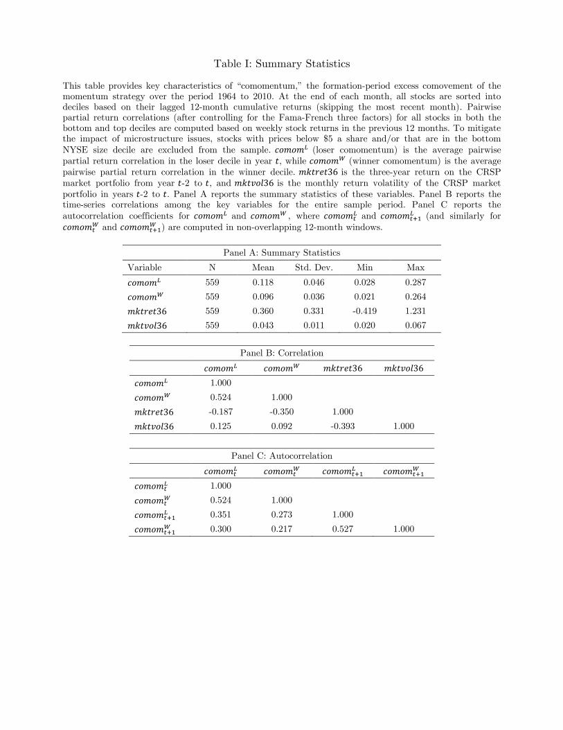
Table I: Summary Statistics

This table provides key characteristics of “comomentum,” the formation-period excess comovement of the

momentum strategy over the period 1964 to 2010. At the end of each month, all stocks are sorted into

deciles based on their lagged 12-month cumulative returns (skipping the most recent month). Pairwise

partial return correlations (after controlling for the Fama-French three factors) for all stocks in both the

bottom and top deciles are computed based on weekly stock returns in the previous 12 months. To mitigate

the impact of microstructure issues, stocks with prices below $5 a share and/or that are in the bottom

NYSE size decile are excluded from the sample. (loser comomentum) is the average pairwise

partial return correlation in the loser decile in year , while (winner comomentum) is the average

pairwise partial return correlation in the winner decile. is the three-year return on the CRSP

market portfolio from year -2 to , and is the monthly return volatility of the CRSP market

portfolio in years -2 to . Panel A reports the summary statistics of these variables. Panel B reports the time-series correlations among the key variables for the entire sample period. Panel C reports the

autocorrelation coefficients for and , where and

(and similarly for

and

) are computed in non-overlapping 12-month windows.

Panel A: Summary Statistics

Variable N Mean Std. Dev. Min Max

559 0.118 0.046 0.028 0.287

559 0.096 0.036 0.021 0.264

559 0.360 0.331 -0.419 1.231

559 0.043 0.011 0.020 0.067

Panel B: Correlation

1.000

0.524 1.000

-0.187 -0.350 1.000

0.125 0.092 -0.393 1.000

Panel C: Autocorrelation

1.000

0.524 1.000

0.351 0.273 1.000

0.300 0.217 0.527 1.000

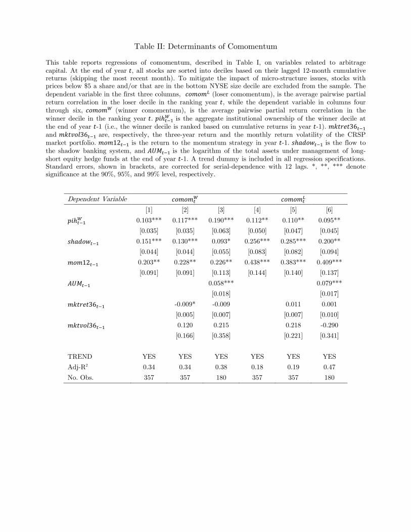
Table II: Determinants of Comomentum

This table reports regressions of comomentum, described in Table I, on variables related to arbitrage

capital. At the end of year , all stocks are sorted into deciles based on their lagged 12-month cumulative returns (skipping the most recent month). To mitigate the impact of micro-structure issues, stocks with

prices below $5 a share and/or that are in the bottom NYSE size decile are excluded from the sample. The

dependent variable in the first three columns, (loser comomentum), is the average pairwise partial

return correlation in the loser decile in the ranking year , while the dependent variable in columns four

through six, (winner comomentum), is the average pairwise partial return correlation in the

winner decile in the ranking year . is the aggregate institutional ownership of the winner decile at

the end of year -1 (i.e., the winner decile is ranked based on cumulative returns in year -1).

and are, respectively, the three-year return and the monthly return volatility of the CRSP

market portfolio. is the return to the momentum strategy in year -1. is the flow to

the shadow banking system, and is the logarithm of the total assets under management of long-

short equity hedge funds at the end of year -1. A trend dummy is included in all regression specifications. Standard errors, shown in brackets, are corrected for serial-dependence with 12 lags. *, **, *** denote

significance at the 90%, 95%, and 99% level, respectively.

Dependent Variable

[1] [2] [3] [4] [5] [6]

0.103*** 0.117*** 0.190*** 0.112** 0.110** 0.095**

[0.035] [0.035] [0.063] [0.050] [0.047] [0.045]

0.151*** 0.130*** 0.093* 0.256*** 0.285*** 0.200**

[0.044] [0.044] [0.055] [0.083] [0.082] [0.094]

0.203** 0.228** 0.226** 0.438*** 0.383*** 0.409***

[0.091] [0.091] [0.113] [0.144] [0.140] [0.137]

0.058***

0.079***

[0.018]

[0.017]

-0.009* -0.009

0.011 0.001

[0.005] [0.007]

[0.007] [0.010]

0.120 0.215

0.218 -0.290

[0.166] [0.358]

[0.221] [0.341]

TREND YES YES YES YES YES YES

Adj-R2 0.34 0.34 0.38 0.18 0.19 0.47

No. Obs. 357 357 180 357 357 180

Table III: Forecasting Momentum Returns with Comomentum

This table reports returns to the momentum strategy as a function of lagged comomentum. At the end of

each month, all stocks are sorted into deciles based on their lagged 12-month cumulative returns (skipping

the most recent month). Stocks with prices below $5 a share and/or that are in the bottom NYSE size

decile are excluded from the sample. All months are then classified into five groups based on , the average pairwise partial return correlation in the loser decile ranked in the previous 12 months. Reported

below are the returns to the momentum strategy (i.e., long the value-weight winner decile and short the

value-weight loser decile) in each of the three years after portfolio formation during 1965 to 2010, following

low to high . Year zero is the portfolio ranking period. Panels A and B report, respectively, the average monthly return and the average Fama-French three-factor alpha of the momentum strategy,

respectively. “5-1” is the difference in monthly returns to the momentum strategy following high vs. low

. “OLS” is the slope coefficient from the regression of monthly momentum returns on ranks of

. T-statistics, shown in parentheses, are computed based on standard errors corrected for serial-dependence with 12 lags. 5% statistical significance is indicated in bold.

Panel A: Raw Momentum Returns

Year 0 Year 1 Year 2 Year 3

Rank No Obs. Estimate t-stat Estimate t-stat Estimate t-stat Estimate t-stat

1 110 8.84% (29.59) 0.69% (4.56) 0.14% (0.56) -0.05% (-0.21)

2 111 8.94% (24.66) 1.05% (6.67) -0.27% (-1.09) -0.54% (-2.64)

3 111 9.19% (15.66) 0.73% (3.15) -0.51% (-1.66) -0.52% (-2.89)

4 111 9.51% (16.57) 0.44% (1.54) -0.58% (-2.39) -0.46% (-1.81)

5 111 11.24% (13.58) -0.18% (-0.35) -1.05% (-2.81) 0.16% (0.45)

5-1 2.40% (2.76) -0.87% (-2.11) -1.20% (-2.72) 0.21% (0.61)

OLS 0.006 (2.83) -0.002 (-2.02) -0.003 (-2.81) 0.000 (0.45)

Panel B: Three-Factor Adjusted Momentum Returns

Year 0 Year 1 Year 2 Year 3

Rank No Obs. Estimate t-stat Estimate t-stat Estimate t-stat Estimate t-stat

1 110 8.45% (24.33) 0.70% (3.63) -0.03% (-0.10) -0.15% (-1.07)

2 111 8.53% (19.67) 1.06% (5.00) -0.44% (-2.33) -0.87% (-3.46)

3 111 8.74% (13.91) 0.61% (3.22) -0.67% (-3.17) -0.70% (-2.74)

4 111 9.13% (14.31) 0.35% (1.53) -0.61% (-2.35) -0.69% (-2.28)

5 111 10.81% (13.14) -0.08% (-0.18) -0.80% (-2.31) 0.14% (0.90)

5-1 2.37% (2.64) -0.79% (-2.22) -0.78% (-2.33) 0.28% (0.95)

OLS 0.006 (2.65) -0.002 (-2.09) -0.002 (-2.38) 0.000 (0.64)

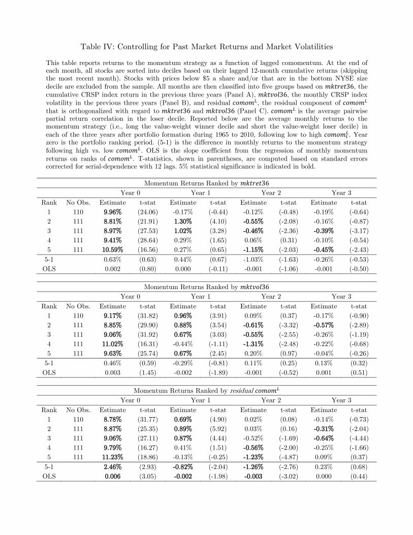
Table IV: Controlling for Past Market Returns and Market Volatilities

This table reports returns to the momentum strategy as a function of lagged comomentum. At the end of

each month, all stocks are sorted into deciles based on their lagged 12-month cumulative returns (skipping

the most recent month). Stocks with prices below $5 a share and/or that are in the bottom NYSE size

decile are excluded from the sample. All months are then classified into five groups based on , the

cumulative CRSP index return in the previous three years (Panel A), , the monthly CRSP index

volatility in the previous three years (Panel B), and residual , the residual component of

that is orthogonalized with regard to and (Panel C). is the average pairwise partial return correlation in the loser decile. Reported below are the average monthly returns to the

momentum strategy (i.e., long the value-weight winner decile and short the value-weight loser decile) in

each of the three years after portfolio formation during 1965 to 2010, following low to high . Year

zero is the portfolio ranking period. (5-1) is the difference in monthly returns to the momentum strategy

following high vs. low . OLS is the slope coefficient from the regression of monthly momentum

returns on ranks of . T-statistics, shown in parentheses, are computed based on standard errors corrected for serial-dependence with 12 lags. 5% statistical significance is indicated in bold.

Momentum Returns Ranked by

Year 0 Year 1 Year 2 Year 3

Rank No Obs. Estimate t-stat Estimate t-stat Estimate t-stat Estimate t-stat

1 110 9.96% (24.06) -0.17% (-0.44) -0.12% (-0.48) -0.19% (-0.64)

2 111 8.81% (21.91) 1.30% (4.10) -0.55% (-2.08) -0.16% (-0.87)

3 111 8.97% (27.53) 1.02% (3.28) -0.46% (-2.36) -0.39% (-3.17)

4 111 9.41% (28.64) 0.29% (1.65) 0.06% (0.31) -0.10% (-0.54)

5 111 10.59% (16.56) 0.27% (0.65) -1.15% (-2.03) -0.45% (-2.43)

5-1 0.63% (0.63) 0.44% (0.67) -1.03% (-1.63) -0.26% (-0.53)

OLS 0.002 (0.80) 0.000 (-0.11) -0.001 (-1.06) -0.001 (-0.50)

Momentum Returns Ranked by

Year 0 Year 1 Year 2 Year 3

Rank No Obs. Estimate t-stat Estimate t-stat Estimate t-stat Estimate t-stat

1 110 9.17% (31.82) 0.96% (3.91) 0.09% (0.37) -0.17% (-0.90)

2 111 8.85% (29.90) 0.88% (3.54) -0.61% (-3.32) -0.57% (-2.89)

3 111 9.06% (31.92) 0.67% (3.03) -0.55% (-2.55) -0.26% (-1.19)

4 111 11.02% (16.31) -0.44% (-1.11) -1.31% (-2.48) -0.22% (-0.68)

5 111 9.63% (25.74) 0.67% (2.45) 0.20% (0.97) -0.04% (-0.26)

5-1 0.46% (0.59) -0.29% (-0.81) 0.11% (0.25) 0.13% (0.32)

OLS 0.003 (1.45) -0.002 (-1.89) -0.001 (-0.52) 0.001 (0.51)

Momentum Returns Ranked by residual

Year 0 Year 1 Year 2 Year 3

Rank No Obs. Estimate t-stat Estimate t-stat Estimate t-stat Estimate t-stat

1 110 8.78% (31.77) 0.69% (4.90) 0.02% (0.08) -0.14% (-0.73)

2 111 8.87% (25.35) 0.89% (5.92) 0.03% (0.16) -0.31% (-2.04)

3 111 9.06% (27.11) 0.87% (4.44) -0.52% (-1.69) -0.64% (-4.44)

4 111 9.79% (16.27) 0.41% (1.51) -0.56% (-2.00) -0.25% (-1.66)

5 111 11.23% (18.86) -0.13% (-0.25) -1.23% (-4.87) 0.09% (0.37)

5-1 2.46% (2.93) -0.82% (-2.04) -1.26% (-2.76) 0.23% (0.68)

OLS 0.006 (3.05) -0.002 (-1.98) -0.003 (-3.02) 0.000 (0.44)

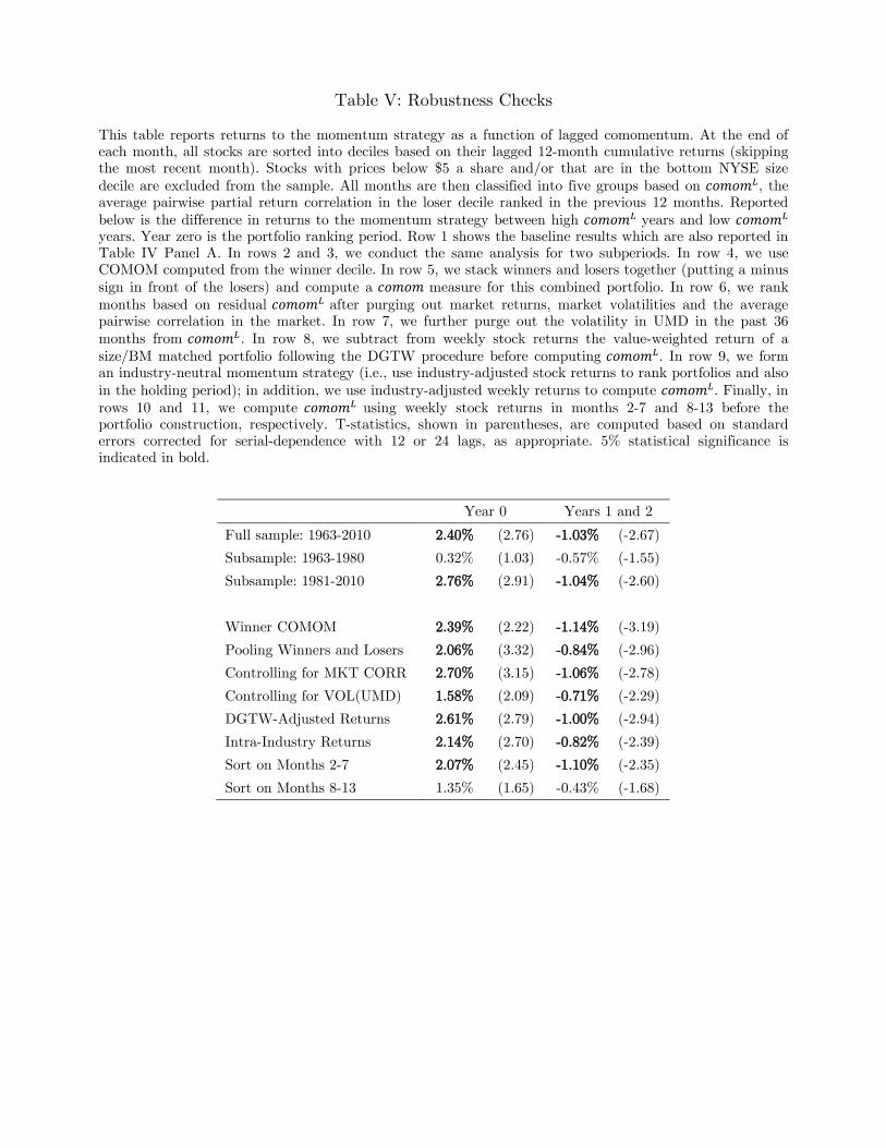
Table V: Robustness Checks

This table reports returns to the momentum strategy as a function of lagged comomentum. At the end of

each month, all stocks are sorted into deciles based on their lagged 12-month cumulative returns (skipping

the most recent month). Stocks with prices below $5 a share and/or that are in the bottom NYSE size

decile are excluded from the sample. All months are then classified into five groups based on , the average pairwise partial return correlation in the loser decile ranked in the previous 12 months. Reported

below is the difference in returns to the momentum strategy between high years and low years. Year zero is the portfolio ranking period. Row 1 shows the baseline results which are also reported in

Table IV Panel A. In rows 2 and 3, we conduct the same analysis for two subperiods. In row 4, we use

COMOM computed from the winner decile. In row 5, we stack winners and losers together (putting a minus

sign in front of the losers) and compute a measure for this combined portfolio. In row 6, we rank

months based on residual after purging out market returns, market volatilities and the average pairwise correlation in the market. In row 7, we further purge out the volatility in UMD in the past 36

months from . In row 8, we subtract from weekly stock returns the value-weighted return of a

size/BM matched portfolio following the DGTW procedure before computing . In row 9, we form an industry-neutral momentum strategy (i.e., use industry-adjusted stock returns to rank portfolios and also

in the holding period); in addition, we use industry-adjusted weekly returns to compute . Finally, in

rows 10 and 11, we compute using weekly stock returns in months 2-7 and 8-13 before the portfolio construction, respectively. T-statistics, shown in parentheses, are computed based on standard

errors corrected for serial-dependence with 12 or 24 lags, as appropriate. 5% statistical significance is

indicated in bold.

Year 0 Years 1 and 2

Full sample: 1963-2010 2.40% (2.76) -1.03% (-2.67)

Subsample: 1963-1980 0.32% (1.03) -0.57% (-1.55)

Subsample: 1981-2010 2.76% (2.91) -1.04% (-2.60)

Winner COMOM 2.39% (2.22) -1.14% (-3.19)

Pooling Winners and Losers 2.06% (3.32) -0.84% (-2.96)

Controlling for MKT CORR 2.70% (3.15) -1.06% (-2.78)

Controlling for VOL(UMD) 1.58% (2.09) -0.71% (-2.29)

DGTW-Adjusted Returns 2.61% (2.79) -1.00% (-2.94)

Intra-Industry Returns 2.14% (2.70) -0.82% (-2.39)

Sort on Months 2-7 2.07% (2.45) -1.10% (-2.35)

Sort on Months 8-13 1.35% (1.65) -0.43% (-1.68)

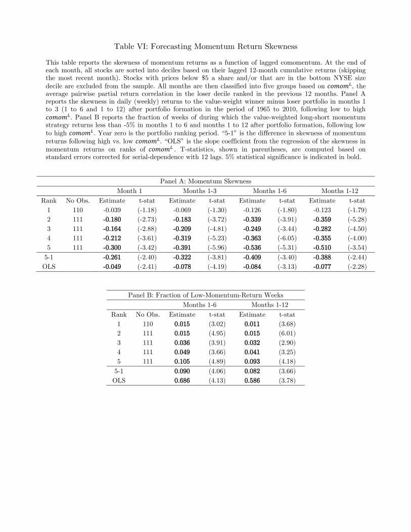
Table VI: Forecasting Momentum Return Skewness

This table reports the skewness of momentum returns as a function of lagged comomentum. At the end of

each month, all stocks are sorted into deciles based on their lagged 12-month cumulative returns (skipping

the most recent month). Stocks with prices below $5 a share and/or that are in the bottom NYSE size

decile are excluded from the sample. All months are then classified into five groups based on , the average pairwise partial return correlation in the loser decile ranked in the previous 12 months. Panel A

reports the skewness in daily (weekly) returns to the value-weight winner minus loser portfolio in months 1

to 3 (1 to 6 and 1 to 12) after portfolio formation in the period of 1965 to 2010, following low to high

. Panel B reports the fraction of weeks of during which the value-weighted long-short momentum strategy returns less than -5% in months 1 to 6 and months 1 to 12 after portfolio formation, following low

to high . Year zero is the portfolio ranking period. “5-1” is the difference in skewness of momentum

returns following high vs. low . “OLS” is the slope coefficient from the regression of the skewness in

momentum returns on ranks of . T-statistics, shown in parentheses, are computed based on standard errors corrected for serial-dependence with 12 lags. 5% statistical significance is indicated in bold.

Panel A: Momentum Skewness

Month 1 Months 1-3 Months 1-6 Months 1-12

Rank No Obs. Estimate t-stat Estimate t-stat Estimate t-stat Estimate t-stat

1 110 -0.039 (-1.18) -0.069 (-1.30) -0.126 (-1.80) -0.123 (-1.79)

2 111 -0.180 (-2.73) -0.183 (-3.72) -0.339 (-3.91) -0.359 (-5.28)

3 111 -0.164 (-2.88) -0.209 (-4.81) -0.249 (-3.44) -0.282 (-4.50)

4 111 -0.212 (-3.61) -0.319 (-5.23) -0.363 (-6.05) -0.355 (-4.00)

5 111 -0.300 (-3.42) -0.391 (-5.96) -0.536 (-5.31) -0.510 (-3.54)

5-1 -0.261 (-2.40) -0.322 (-3.81) -0.409 (-3.40) -0.388 (-2.44)

OLS -0.049 (-2.41) -0.078 (-4.19) -0.084 (-3.13) -0.077 (-2.28)

Panel B: Fraction of Low-Momentum-Return Weeks

Months 1-6 Months 1-12

Rank No Obs. Estimate t-stat Estimate t-stat

1 110 0.015 (3.02) 0.011 (3.68)

2 111 0.015 (4.95) 0.015 (6.01)

3 111 0.036 (3.91) 0.032 (2.90)

4 111 0.049 (3.66) 0.041 (3.25)

5 111 0.105 (4.89) 0.093 (4.18)

5-1 0.090 (4.06) 0.082 (3.66)

OLS 0.686 (4.13) 0.586 (3.78)

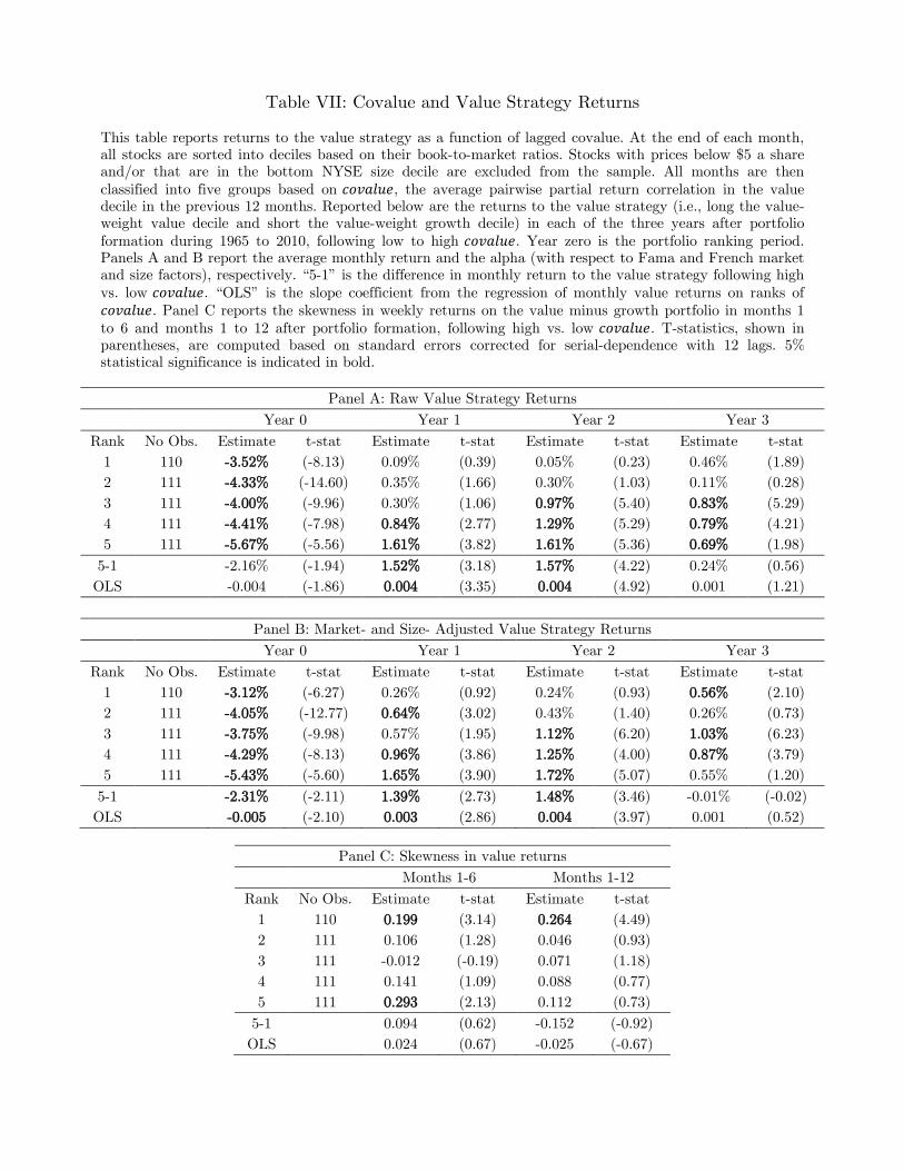
Table VII: Covalue and Value Strategy Returns

This table reports returns to the value strategy as a function of lagged covalue. At the end of each month,

all stocks are sorted into deciles based on their book-to-market ratios. Stocks with prices below $5 a share

and/or that are in the bottom NYSE size decile are excluded from the sample. All months are then

classified into five groups based on , the average pairwise partial return correlation in the value decile in the previous 12 months. Reported below are the returns to the value strategy (i.e., long the value-

weight value decile and short the value-weight growth decile) in each of the three years after portfolio

formation during 1965 to 2010, following low to high . Year zero is the portfolio ranking period. Panels A and B report the average monthly return and the alpha (with respect to Fama and French market

and size factors), respectively. “5-1” is the difference in monthly return to the value strategy following high

vs. low . “OLS” is the slope coefficient from the regression of monthly value returns on ranks of

. Panel C reports the skewness in weekly returns on the value minus growth portfolio in months 1

to 6 and months 1 to 12 after portfolio formation, following high vs. low . T-statistics, shown in

parentheses, are computed based on standard errors corrected for serial-dependence with 12 lags. 5%

statistical significance is indicated in bold.

Panel A: Raw Value Strategy Returns

Year 0 Year 1 Year 2 Year 3

Rank No Obs. Estimate t-stat Estimate t-stat Estimate t-stat Estimate t-stat

1 110 -3.52% (-8.13) 0.09% (0.39) 0.05% (0.23) 0.46% (1.89)

2 111 -4.33% (-14.60) 0.35% (1.66) 0.30% (1.03) 0.11% (0.28)

3 111 -4.00% (-9.96) 0.30% (1.06) 0.97% (5.40) 0.83% (5.29)

4 111 -4.41% (-7.98) 0.84% (2.77) 1.29% (5.29) 0.79% (4.21)

5 111 -5.67% (-5.56) 1.61% (3.82) 1.61% (5.36) 0.69% (1.98)

5-1 -2.16% (-1.94) 1.52% (3.18) 1.57% (4.22) 0.24% (0.56)

OLS -0.004 (-1.86) 0.004 (3.35) 0.004 (4.92) 0.001 (1.21)

Panel B: Market- and Size- Adjusted Value Strategy Returns

Year 0 Year 1 Year 2 Year 3

Rank No Obs. Estimate t-stat Estimate t-stat Estimate t-stat Estimate t-stat

1 110 -3.12% (-6.27) 0.26% (0.92) 0.24% (0.93) 0.56% (2.10)

2 111 -4.05% (-12.77) 0.64% (3.02) 0.43% (1.40) 0.26% (0.73)

3 111 -3.75% (-9.98) 0.57% (1.95) 1.12% (6.20) 1.03% (6.23)

4 111 -4.29% (-8.13) 0.96% (3.86) 1.25% (4.00) 0.87% (3.79)

5 111 -5.43% (-5.60) 1.65% (3.90) 1.72% (5.07) 0.55% (1.20)

5-1 -2.31% (-2.11) 1.39% (2.73) 1.48% (3.46) -0.01% (-0.02)

OLS -0.005 (-2.10) 0.003 (2.86) 0.004 (3.97) 0.001 (0.52)

Panel C: Skewness in value returns

Months 1-6 Months 1-12

Rank No Obs. Estimate t-stat Estimate t-stat

1 110 0.199 (3.14) 0.264 (4.49)

2 111 0.106 (1.28) 0.046 (0.93)

3 111 -0.012 (-0.19) 0.071 (1.18)

4 111 0.141 (1.09) 0.088 (0.77)

5 111 0.293 (2.13) 0.112 (0.73)

5-1 0.094 (0.62) -0.152 (-0.92)

OLS 0.024 (0.67) -0.025 (-0.67)

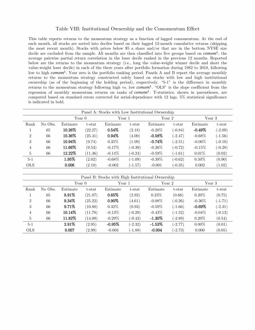
Table VIII: Institutional Ownership and the Comomentum Effect

This table reports returns to the momentum strategy as a function of lagged comomentum. At the end of

each month, all stocks are sorted into deciles based on their lagged 12-month cumulative returns (skipping

the most recent month). Stocks with prices below $5 a share and/or that are in the bottom NYSE size

decile are excluded from the sample. All months are then classified into five groups based on , the average pairwise partial return correlation in the loser decile ranked in the previous 12 months. Reported

below are the returns to the momentum strategy (i.e., long the value-weight winner decile and short the

value-weight loser decile) in each of the three years after portfolio formation during 1982 to 2010, following

low to high . Year zero is the portfolio ranking period. Panels A and B report the average monthly returns to the momentum strategy constructed solely based on stocks with low and high institutional

ownership (as of the beginning of the holding period), respectively. “5-1” is the difference in monthly

returns to the momentum strategy following high vs. low . “OLS” is the slope coefficient from the

regression of monthly momentum returns on ranks of . T-statistics, shown in parentheses, are computed based on standard errors corrected for serial-dependence with 12 lags. 5% statistical significance

is indicated in bold.

Panel A: Stocks with Low Institutional Ownership

Year 0 Year 1 Year 2 Year 3

Rank No Obs. Estimate t-stat Estimate t-stat Estimate t-stat Estimate t-stat

1 65 10.26% (22.27) 0.54% (2.18) -0.20% (-0.84) -0.49% (-2.09)

2 66 10.36% (25.41) 0.94% (4.00) -0.58% (-2.47) -0.68% (-1.56)

3 66 10.94% (9.74) 0.35% (1.09) -0.74% (-2.51) -0.06% (-0.10)

4 66 11.66% (9.53) -0.17% (-0.39) -0.26% (-0.72) -0.15% (-0.28)

5 66 12.22% (11.46) -0.14% (-0.24) -0.59% (-1.61) 0.01% (0.02)

5-1 1.95% (2.02) -0.68% (-1.09) -0.39% (-0.62) 0.50% (0.90)

OLS 0.006 (2.10) -0.002 (-1.57) -0.001 (-0.35) 0.002 (1.02)

Panel B: Stocks with High Institutional Ownership

Year 0 Year 1 Year 2 Year 3

Rank No Obs. Estimate t-stat Estimate t-stat Estimate t-stat Estimate t-stat

1 65 8.91% (21.87) 0.65% (2.92) 0.23% (0.66) 0.20% (0.75)

2 66 9.34% (25.22) 0.90% (4.61) -0.08% (-0.26) -0.36% (-1.71)

3 66 9.71% (10.80) 0.32% (0.93) -0.59% (-1.66) -0.69% (-2.31)

4 66 10.14% (11.78) -0.13% (-0.29) -0.43% (-1.52) -0.04% (-0.13)

5 66 11.82% (14.09) -0.29% (-0.43) -1.30% (-2.89) 0.20% (0.54)

5-1 2.91% (2.95) -0.95% (-2.32) -1.53% (-2.77) 0.00% (0.01)

OLS 0.007 (2.99) -0.003 (-1.88) -0.004 (-2.73) 0.000 (0.05)

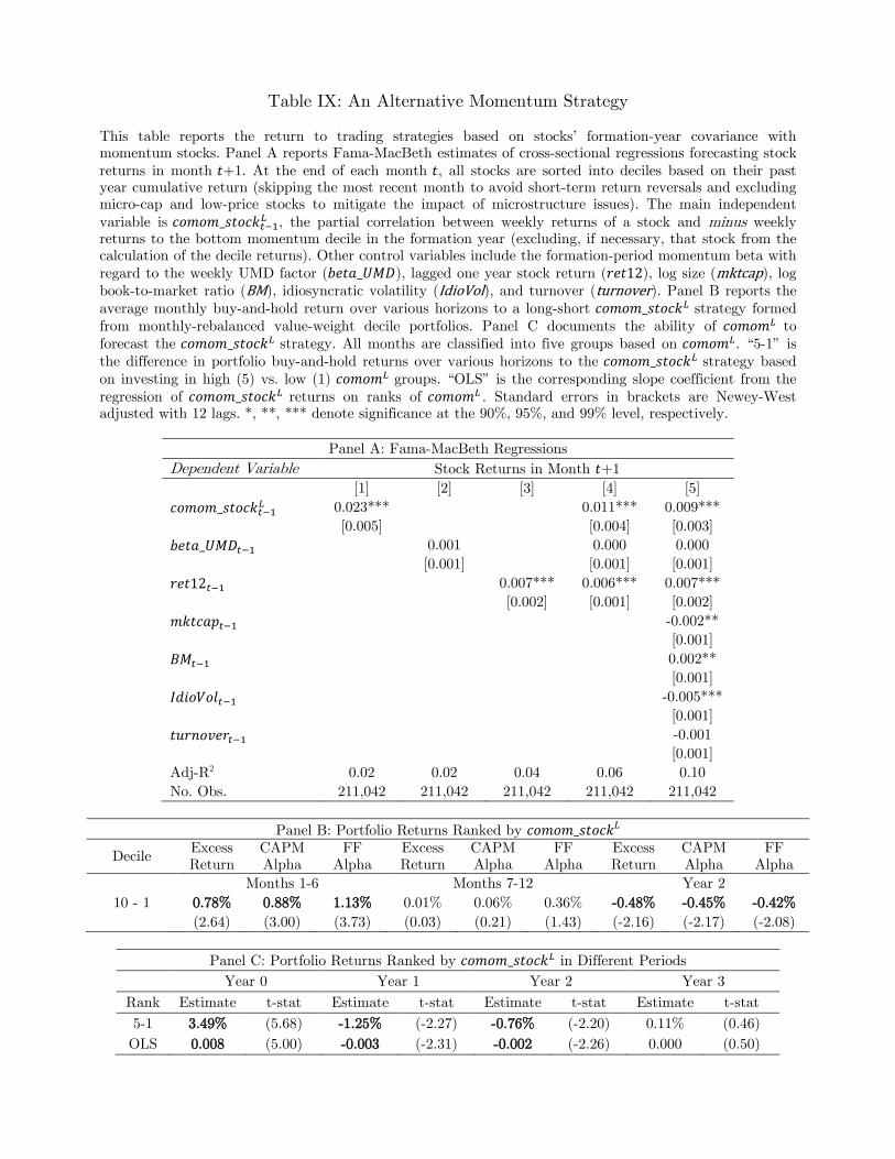
Table IX: An Alternative Momentum Strategy

This table reports the return to trading strategies based on stocks’ formation-year covariance with

momentum stocks. Panel A reports Fama-MacBeth estimates of cross-sectional regressions forecasting stock

returns in month +1. At the end of each month , all stocks are sorted into deciles based on their past year cumulative return (skipping the most recent month to avoid short-term return reversals and excluding

micro-cap and low-price stocks to mitigate the impact of microstructure issues). The main independent

variable is , the partial correlation between weekly returns of a stock and minus weekly

returns to the bottom momentum decile in the formation year (excluding, if necessary, that stock from the

calculation of the decile returns). Other control variables include the formation-period momentum beta with

regard to the weekly UMD factor ( ), lagged one year stock return ( ), log size (mktcap), log

book-to-market ratio (BM), idiosyncratic volatility (IdioVol), and turnover (turnover). Panel B reports the

average monthly buy-and-hold return over various horizons to a long-short strategy formed

from monthly-rebalanced value-weight decile portfolios. Panel C documents the ability of to

forecast the strategy. All months are classified into five groups based on . “5-1” is

the difference in portfolio buy-and-hold returns over various horizons to the strategy based

on investing in high (5) vs. low (1) groups. “OLS” is the corresponding slope coefficient from the

regression of returns on ranks of . Standard errors in brackets are Newey-West adjusted with 12 lags. *, **, *** denote significance at the 90%, 95%, and 99% level, respectively.

Panel A: Fama-MacBeth Regressions

Dependent Variable Stock Returns in Month +1

[1] [2] [3] [4] [5]

0.023***

0.011*** 0.009***

[0.005]

[0.004] [0.003]

0.001 0.000 0.000

[0.001] [0.001] [0.001]

0.007*** 0.006*** 0.007***

[0.002] [0.001] [0.002]

-0.002**

[0.001]

0.002**

[0.001]

-0.005***

[0.001]

-0.001

[0.001]

Adj-R2 0.02 0.02 0.04 0.06 0.10

No. Obs. 211,042 211,042 211,042 211,042 211,042

Panel B: Portfolio Returns Ranked by

Decile Excess

Return

CAPM

Alpha

FF

Alpha

Excess

Return

CAPM

Alpha

FF

Alpha

Excess

Return

CAPM

Alpha

FF

Alpha

Months 1-6 Months 7-12 Year 2

10 - 1 0.78% 0.88% 1.13% 0.01% 0.06% 0.36% -0.48% -0.45% -0.42%

(2.64) (3.00) (3.73) (0.03) (0.21) (1.43) (-2.16) (-2.17) (-2.08)

Panel C: Portfolio Returns Ranked by in Different Periods

Year 0 Year 1 Year 2 Year 3

Rank Estimate t-stat Estimate t-stat Estimate t-stat Estimate t-stat

5-1 3.49% (5.68) -1.25% (-2.27) -0.76% (-2.20) 0.11% (0.46)

OLS 0.008 (5.00) -0.003 (-2.31) -0.002 (-2.26) 0.000 (0.50)

Table X: International Evidence

This table reports returns to international momentum strategies as a function of lagged country-specific

comomentum. In Panel A, at the end of each month, stocks in each market are sorted into deciles based on

their lagged 12-month cumulative returns (skipping the most recent month). We then compute a measure as the average pairwise return correlation in the loser decile ranked in the previous 12 months.

CoefEst1 is the regression coefficient of the month momentum return on computed at the end of

month -1, while CoefEst2 is the corresponding regression coefficient, controlling for country-specific market, size, and value factors. We examine the world’s largest 19 stock markets (after the US). We also compute a

value-weight world (excluding the US) momentum strategy (WLD) and forecast that strategy with the

corresponding value-weight world measure. In Panel B, we report the monthly returns to an inter-country (including the US) momentum timing strategy, which goes long country-specific momentum

strategies whose corresponding is in the bottom quintile in the previous month, and short those

country-specific momentum strategies whose corresponding is in the top quintile. We then adjust these monthly returns using world (including the US) market, size, value, and momentum factors. T-

statistics, shown in parentheses, are computed based on standard errors corrected for serial-dependence with

12 lags. 5% statistical significance is indicated in bold.

Panel A: Regression Coefficients in Other Countries

Country No months CoefEst1 CoefEst2

Country No months CeofEst1 CeofEst2

AUS 302 -0.0494 -0.0351

GBR 300 -0.0501 -0.0402

(-0.94) (-0.48)

(-1.87) (-2.11)

AUT 302 -0.0581 -0.0866

HKG 300 -0.0646 -0.0796

(-1.76) (-1.17)

(-3.77) (-2.21)

BEL 300 -0.1025 -0.0946

ITA 300 -0.0108 -0.0239

(-2.40) (-1.95)

(-0.43) (-0.73)

CAN 336 -0.1652 -0.1341

JPN 300 -0.0564 -0.0535

(-2.70) (-2.31)

(-1.63) (-2.54)

CHE 300 -0.0347 -0.0753

NLD 300 -0.0801 -0.0805

(-1.53) (-2.35)

(-2.47) (-2.02)

DEU 300 -0.0546 -0.0957

NOR 297 -0.0096 -0.1090

(-1.72) (-1.82)

(-0.16) (-1.58)

DNK 300 -0.0248 -0.0200

NZL 271 -0.0879 -0.0462

(-1.06) (-0.63)

(-2.15) (-1.67)

ESP 300 -0.0097 -0.0075

SGP 300 -0.0791 -0.1189

(-0.28) (-0.20)

(-2.36) (-3.86)

FIN 300 -0.0110 -0.0046

SWE 300 -0.0107 -0.0091

(-0.29) (-0.12)

(-0.29) (-0.11)

FRA 300 -0.0725 -0.0486

WLD 300 -0.0851 -0.0569

(-2.06) (-1.13)

(-2.60) (-2.68)

Panel B: Long-Short Portfolios of Country Momentum

Quintile No Months Excess Return CAPM Alpha FF Alpha Carhart Alpha

S 300 0.24% 0.36% 0.68% -0.20%

(0.94) (1.49) (2.98) (-0.96)

L 300 1.01% 1.07% 1.49% 0.46%

(3.74) (4.34) (6.00) (3.87)

L-S 300 0.77% 0.71% 0.81% 0.66%

(3.19) (3.04) (3.30) (2.33)

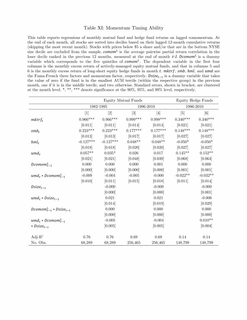
Table XI: Momentum Timing Ability

This table reports regressions of monthly mutual fund and hedge fund returns on lagged comomentum. At

the end of each month, all stocks are sorted into deciles based on their lagged 12-month cumulative returns

(skipping the most recent month). Stocks with prices below $5 a share and/or that are in the bottom NYSE

size decile are excluded from the sample. is the average pairwise partial return correlation in the

loser decile ranked in the previous 12 months, measured at the end of month t-1. is a dummy

variable which corresponds to the five quintiles of . The dependent variable in the first four columns is the monthly excess return of actively-managed equity mutual funds, and that in columns 5 and

6 is the monthly excess return of long-short equity hedge funds in month . , , , and are

the Fama-French three factors and momentum factor, respectively. is a dummy variable that takes the value of zero if the fund is in the smallest AUM tercile (within the respective group) in the previous

month, one if it is in the middle tercile, and two otherwise. Standard errors, shown in bracket, are clustered

at the month level. *, **, *** denote significance at the 90%, 95%, and 99% level, respectively.

Equity Mutual Funds Equity Hedge Funds

1982-1995 1996-2010 1996-2010

[1] [2] [3] [4] [5] [6]

0.966*** 0.966*** 0.999*** 0.998*** 0.340*** 0.340***

[0.011] [0.011] [0.014] [0.014] [0.021] [0.021]

0.223*** 0.223*** 0.177*** 0.177*** 0.148*** 0.148***

[0.013] [0.013] [0.017] [0.017] [0.027] [0.027]

-0.127*** -0.127*** 0.048** 0.048** -0.050* -0.050*

[0.018] [0.018] [0.020] [0.020] [0.027] [0.027]

0.057** 0.035* 0.026 0.017 0.145** 0.152**

[0.021] [0.021] [0.048] [0.039] [0.068] [0.064]

0.000 0.000 0.000 0.001 0.000 0.000

[0.000] [0.000] [0.000] [0.000] [0.001] [0.001]

-0.009 -0.004 -0.005 -0.000 -0.022** -0.032**

[0.010] [0.011] [0.015] [0.018] [0.011] [0.014]

-0.000

-0.000

-0.000

[0.000]

[0.000]

[0.001]

0.021

0.021

-0.006

[0.014]

[0.019]

[0.029]

0.000

0.000

0.000

[0.000]

[0.000]

[0.000]

-0.005

-0.004

0.010**

[0.005]

[0.005]

[0.004]

Adj-R2 0.76 0.76 0.69 0.69 0.14 0.14

No. Obs. 68,289 68,289 256,465 256,465 148,799 148,799

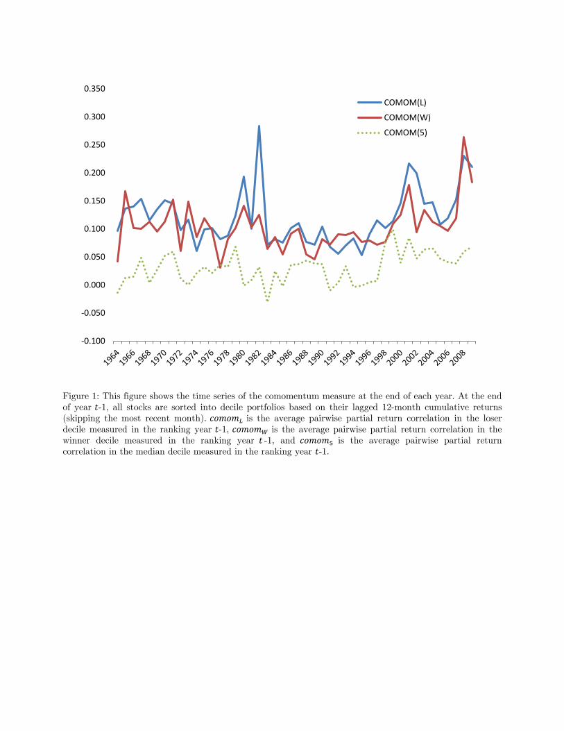
Figure 1: This figure shows the time series of the comomentum measure at the end of each year. At the end

of year -1, all stocks are sorted into decile portfolios based on their lagged 12-month cumulative returns

(skipping the most recent month). is the average pairwise partial return correlation in the loser

decile measured in the ranking year -1, is the average pairwise partial return correlation in the

winner decile measured in the ranking year -1, and is the average pairwise partial return

correlation in the median decile measured in the ranking year -1.

-0.100

-0.050

0.000

0.050

0.100

0.150

0.200

0.250

0.300

0.350

COMOM(L)

COMOM(W)

COMOM(5)

Figure 2: These figures show returns to the momentum strategy as a function of the lagged comomentum

measure. At the end of each month, all stocks are sorted into deciles based on their lagged 12-month

cumulative returns (skipping the most recent month). Stocks with prices below $5 a share and/or are in the

bottom NYSE size decile are excluded from the sample. All months are then classified into five groups

based on , the average pairwise partial return correlation in the loser decile ranked in the previous 12 months. The top panel shows the cumulative returns to a value-weight momentum strategy (i.e., winner

minus loser deciles) in the three years after formation during 1965 to 2010, following low and high . The bottom panel shows the cumulative returns to a value-weight momentum strategy (i.e., winner minus

loser deciles) from the beginning of the formation year to three years post-formation following low and high

.

-0.2

-0.15

-0.1

-0.05

0

0.05

0.1

0.15

1 3 5 7 9 11 13 15 17 19 21 23 25 27 29 31 33 35

Low COMOM

High COMOM

0

0.2

0.4

0.6

0.8

1

1.2

1.4

-11 -9 -7 -5 -3 -1 1 3 5 7 9 11 13 15 17 19 21 23 25 27 29 31 33 35

Low COMOM

High COMOM

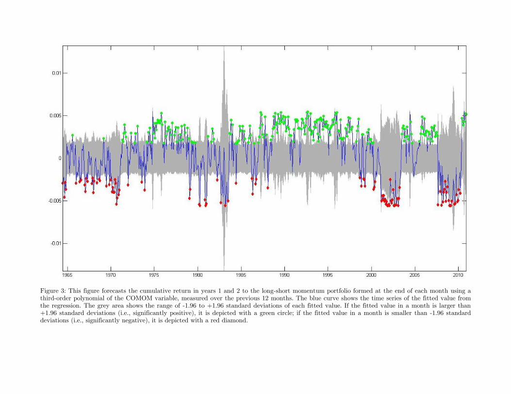
Figure 3: This figure forecasts the cumulative return in years 1 and 2 to the long-short momentum portfolio formed at the end of each month using a

third-order polynomial of the COMOM variable, measured over the previous 12 months. The blue curve shows the time series of the fitted value from

the regression. The grey area shows the range of -1.96 to +1.96 standard deviations of each fitted value. If the fitted value in a month is larger than

+1.96 standard deviations (i.e., significantly positive), it is depicted with a green circle; if the fitted value in a month is smaller than -1.96 standard

deviations (i.e., significantly negative), it is depicted with a red diamond.

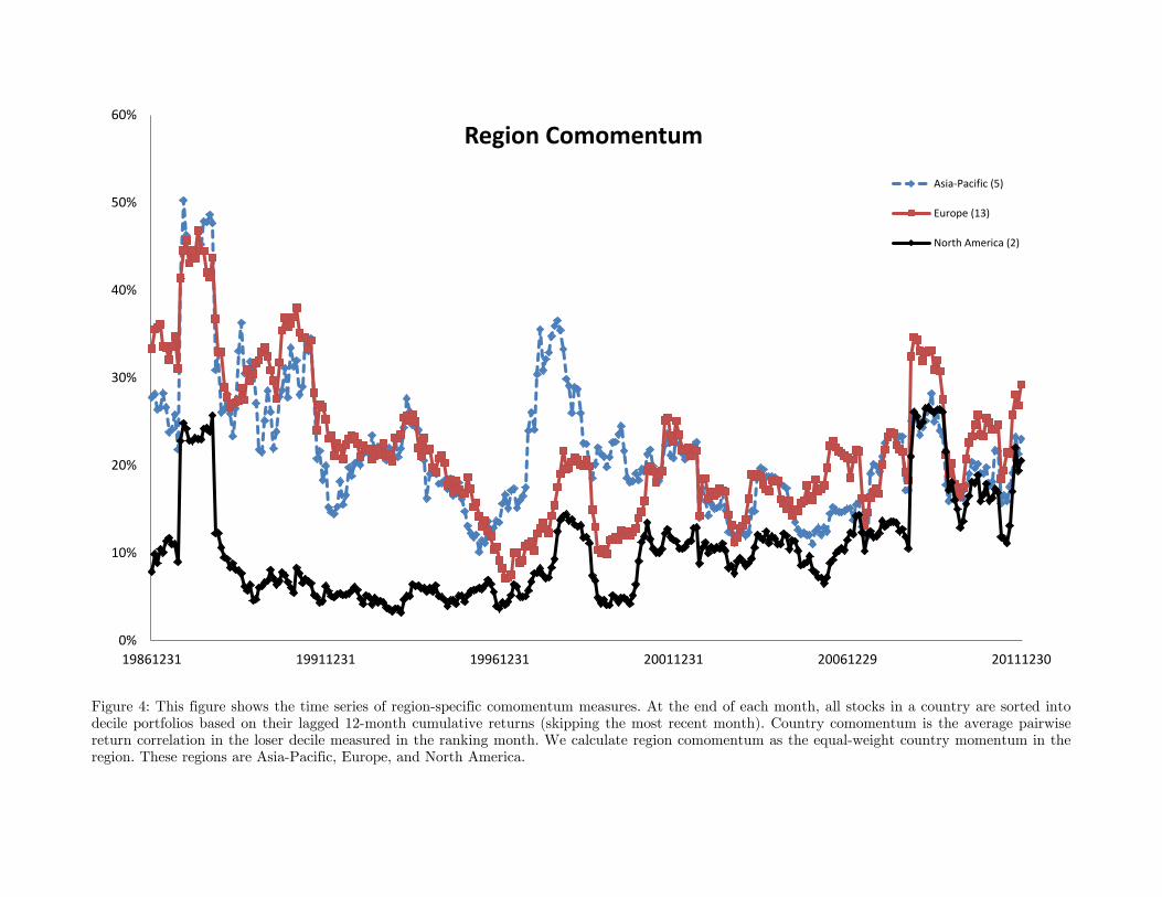
Figure 4: This figure shows the time series of region-specific comomentum measures. At the end of each month, all stocks in a country are sorted into

decile portfolios based on their lagged 12-month cumulative returns (skipping the most recent month). Country comomentum is the average pairwise

return correlation in the loser decile measured in the ranking month. We calculate region comomentum as the equal-weight country momentum in the

region. These regions are Asia-Pacific, Europe, and North America.

0%

10%

20%

30%

40%

50%

60%

19861231 19911231 19961231 20011231 20061229 20111230

Region Comomentum

Asia-Pacific (5)

Europe (13)

North America (2)