comp 122, spring 2004 keys into buckets: lower bounds, linear-time sort, & hashing

Comp 122, Spring 2004

Keys into Buckets: Lower bounds, Linear-time sort, & Hashing

Keys into Buckets: Lower bounds, Linear-time sort, & Hashing

Comp 122linsort - 2 Lin / Devi

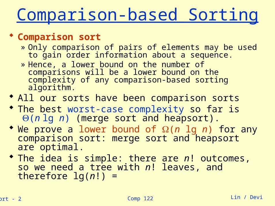
Comparison-based Sorting Comparison sort

» Only comparison of pairs of elements may be used to gain order information about a sequence.

» Hence, a lower bound on the number of comparisons will be a lower bound on the complexity of any comparison-based sorting algorithm.

All our sorts have been comparison sorts The best worst-case complexity so far is (n lg n)

(merge sort and heapsort). We prove a lower bound of (n lg n) for any

comparison sort: merge sort and heapsort are optimal. The idea is simple: there are n! outcomes, so we need a

tree with n! leaves, and therefore lg(n!) =


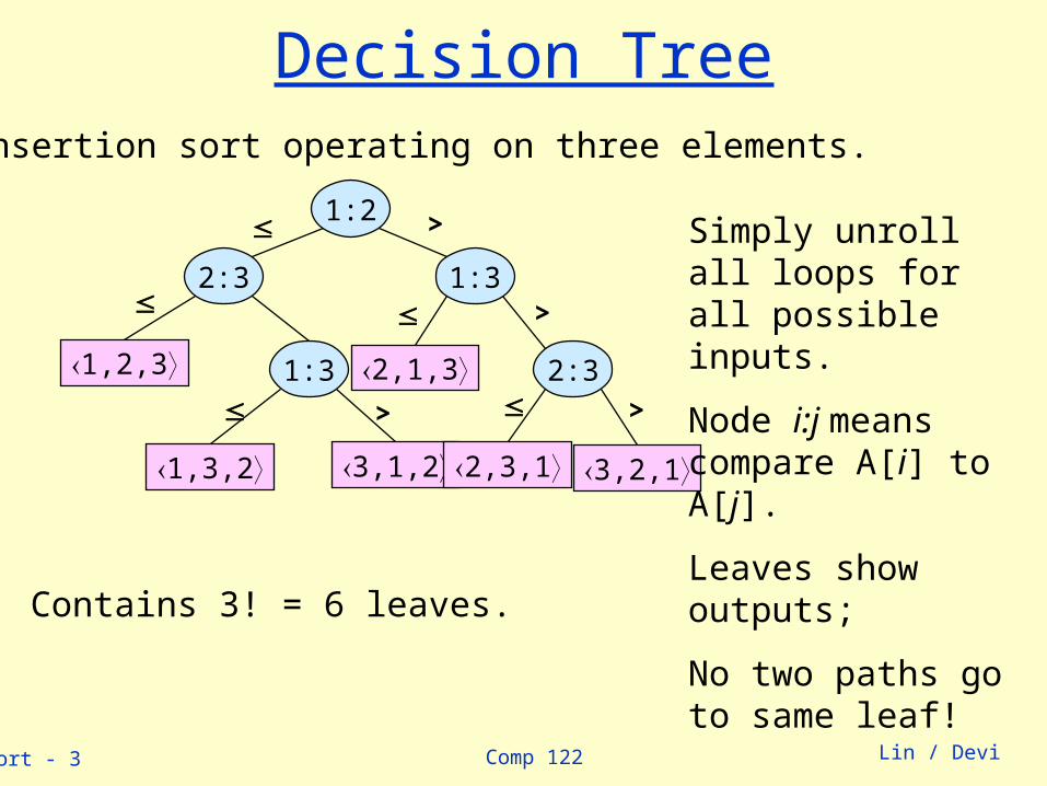
Decision TreeFor insertion sort operating on three elements.

1:2

2:3 1:3

1:3 2:31,2,3

1,3,2 3,1,2

2,1,3

2,3,1 3,2,1

>

>

>>

Contains 3! = 6 leaves.

Simply unroll all loops for all possible inputs.

Node i:j means compare A[i] to A[j].

Leaves show outputs;

No two paths go to same leaf!


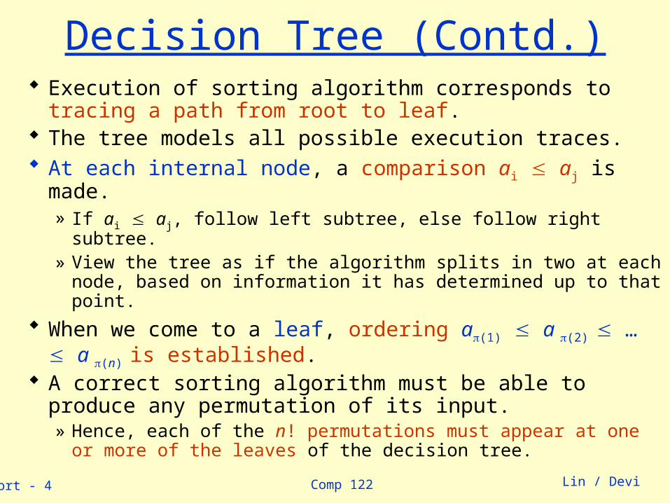
Decision Tree (Contd.) Execution of sorting algorithm corresponds to tracing a

path from root to leaf. The tree models all possible execution traces. At each internal node, a comparison ai aj is made.

» If ai aj, follow left subtree, else follow right subtree.» View the tree as if the algorithm splits in two at each node, based

on information it has determined up to that point.

When we come to a leaf, ordering a(1) a (2) … a (n)

is established. A correct sorting algorithm must be able to produce any

permutation of its input.» Hence, each of the n! permutations must appear at one or more of

the leaves of the decision tree.


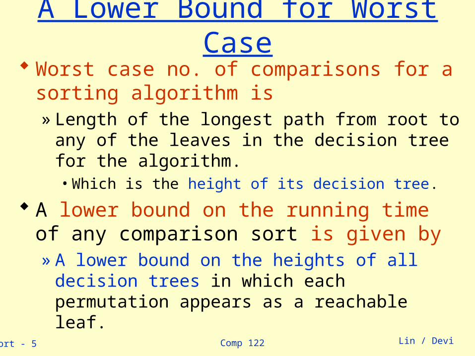
A Lower Bound for Worst CaseWorst case no. of comparisons for a sorting

algorithm is» Length of the longest path from root to any of the

leaves in the decision tree for the algorithm.• Which is the height of its decision tree.

A lower bound on the running time of any comparison sort is given by» A lower bound on the heights of all decision trees in

which each permutation appears as a reachable leaf.


Optimal sorting for three elementsAny sort of six elements has 5 internal nodes.

1:2

2:3 1:3

1:3 2:31,2,3

1,3,2 3,1,2

2,1,3

2,3,1 3,2,1

>

>

>>

There must be a worst-case path of length ≥ 3.


A Lower Bound for Worst Case

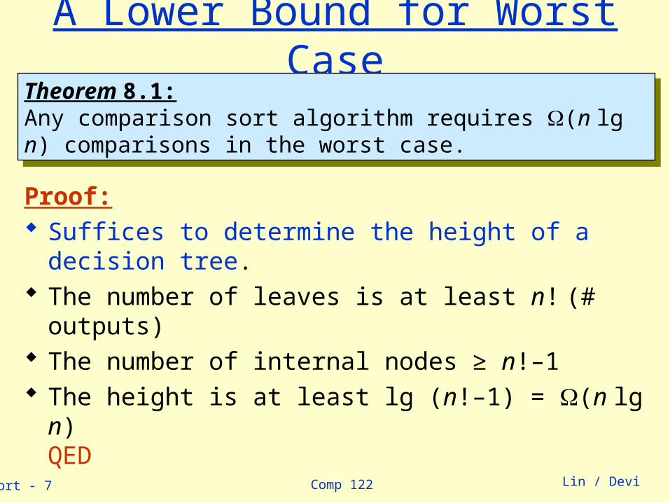
Proof: Suffices to determine the height of a decision tree. The number of leaves is at least n! (# outputs) The number of internal nodes ≥ n!–1 The height is at least lg (n!–1) = (n lg n)

QED

Theorem 8.1:Any comparison sort algorithm requires (n lg n) comparisons in the worst case.

Theorem 8.1:Any comparison sort algorithm requires (n lg n) comparisons in the worst case.


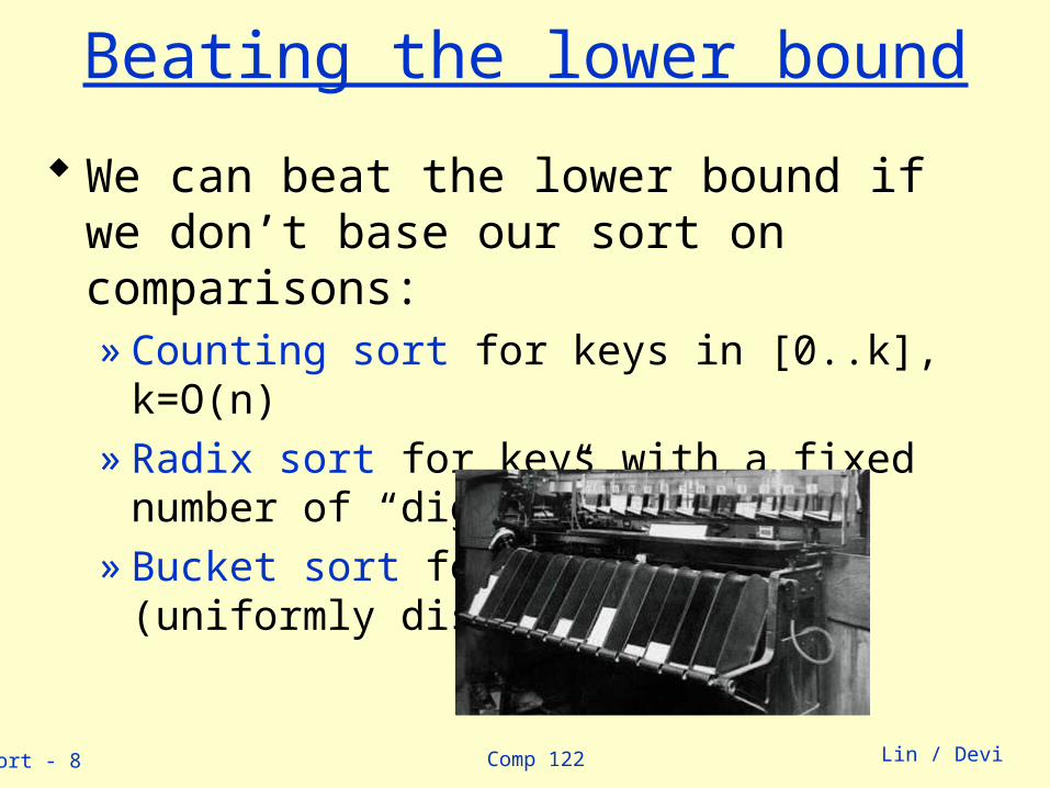
Beating the lower bound

We can beat the lower bound if we don’t base our sort on comparisons:» Counting sort for keys in [0..k], k=O(n)» Radix sort for keys with a fixed number of “digits”» Bucket sort for random keys (uniformly distributed)


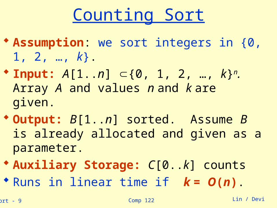
Counting Sort

Assumption: we sort integers in {0, 1, 2, …, k}. Input: A[1..n] {0, 1, 2, …, k}n.

Array A and values n and k are given. Output: B[1..n] sorted. Assume B is already

allocated and given as a parameter. Auxiliary Storage: C[0..k] counts Runs in linear time if k = O(n).


Counting-Sort (A, B, k)

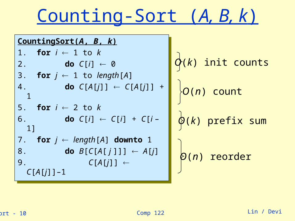
CountingSort(A, B, k)

1. for i 1 to k

2. do C[i] 0

3. for j 1 to length[A]

4. do C[A[j]] C[A[j]] + 1

5. for i 2 to k

6. do C[i] C[i] + C[i –1]

7. for j length[A] downto 1

8. do B[C[A[ j ]]] A[j]

9. C[A[j]] C[A[j]]–1

CountingSort(A, B, k)

1. for i 1 to k

2. do C[i] 0

3. for j 1 to length[A]

4. do C[A[j]] C[A[j]] + 1

5. for i 2 to k

6. do C[i] C[i] + C[i –1]

7. for j length[A] downto 1

8. do B[C[A[ j ]]] A[j]

9. C[A[j]] C[A[j]]–1

O(k) init counts

O(k) prefix sum

O(n) count

O(n) reorder


Radix Sort

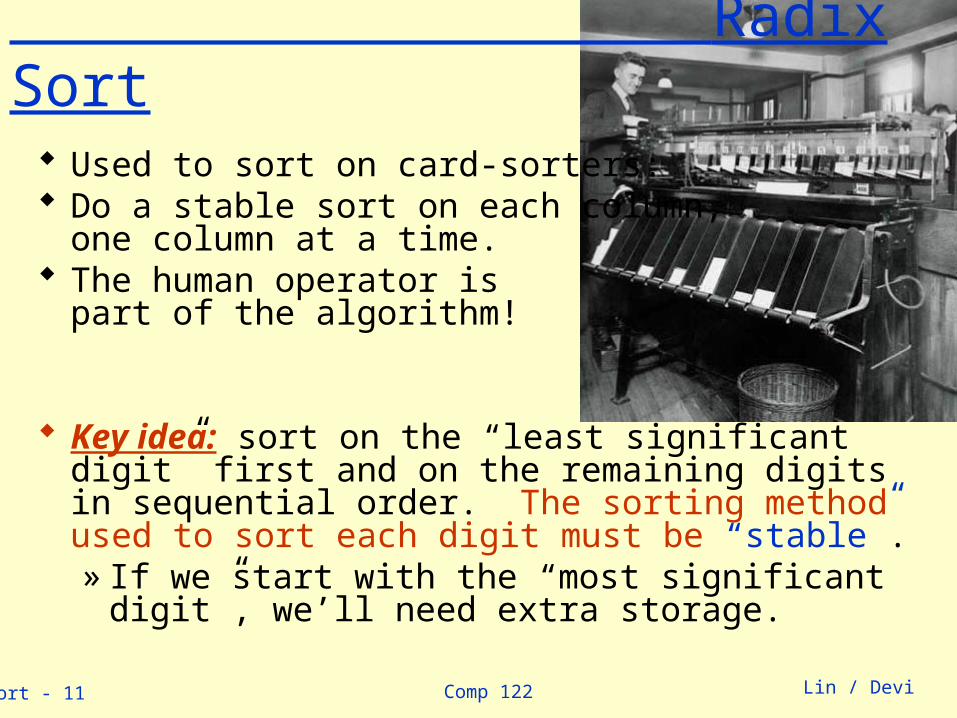
Used to sort on card-sorters: Do a stable sort on each column,

one column at a time. The human operator is

part of the algorithm!

Key idea: sort on the “least significant digit” first and on the remaining digits in sequential order. The sorting method used to sort each digit must be “stable”.» If we start with the “most significant digit”, we’ll

need extra storage.


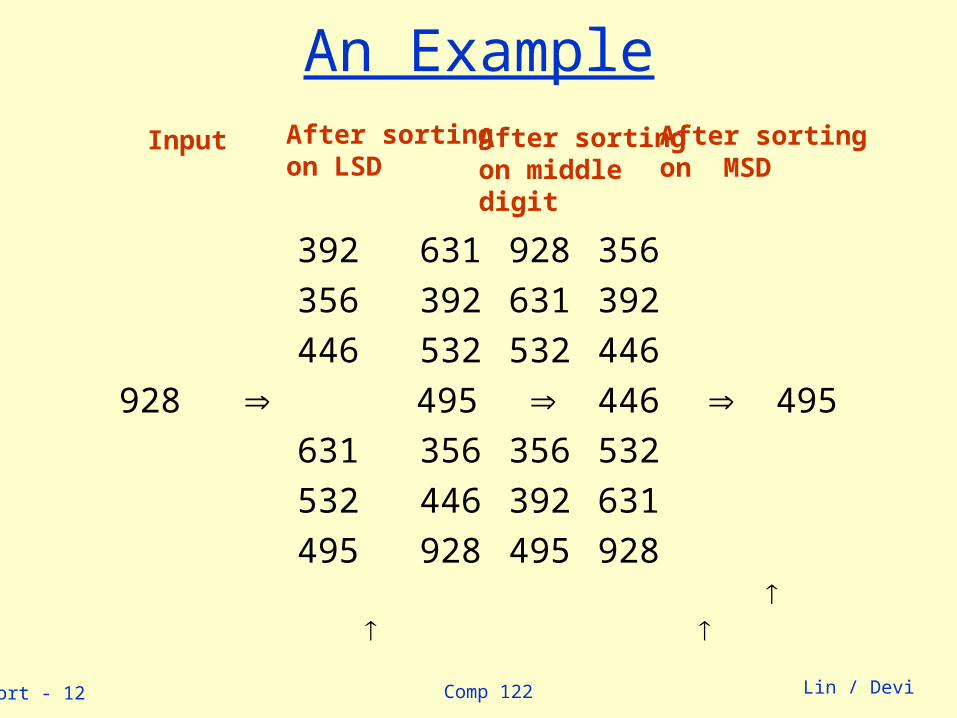
An Example

392 631 928 356

356 392 631 392

446 532 532 446

928 495 446 495

631 356 356 532

532 446 392 631

495 928 495 928

Input After sortingon LSD

After sortingon middle digit

After sortingon MSD


Radix-Sort(A, d)

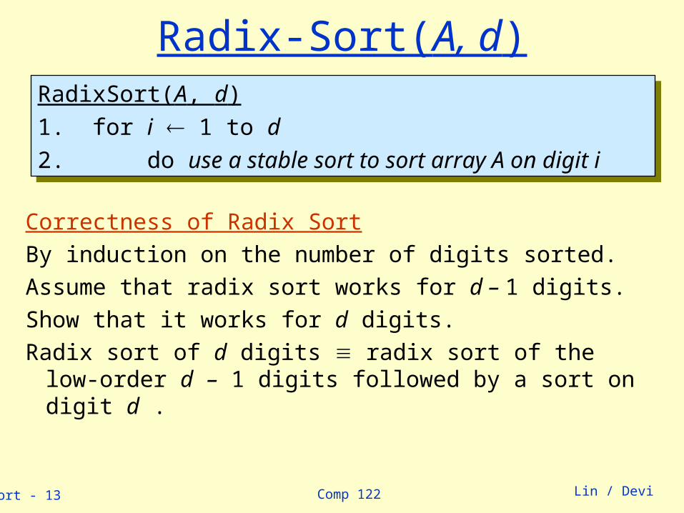
Correctness of Radix Sort

By induction on the number of digits sorted.

Assume that radix sort works for d – 1 digits.

Show that it works for d digits.

Radix sort of d digits radix sort of the low-order d – 1 digits followed by a sort on digit d .

RadixSort(A, d)

1. for i 1 to d

2. do use a stable sort to sort array A on digit i

RadixSort(A, d)

1. for i 1 to d

2. do use a stable sort to sort array A on digit i


Algorithm Analysis

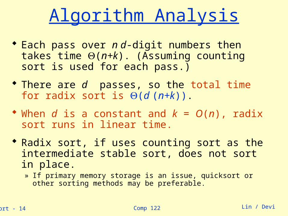
Each pass over n d-digit numbers then takes time (n+k). (Assuming counting sort is used for each pass.)

There are d passes, so the total time for radix sort is (d (n+k)).

When d is a constant and k = O(n), radix sort runs in linear time.

Radix sort, if uses counting sort as the intermediate stable sort, does not sort in place. » If primary memory storage is an issue, quicksort or other sorting methods

may be preferable.


Bucket Sort

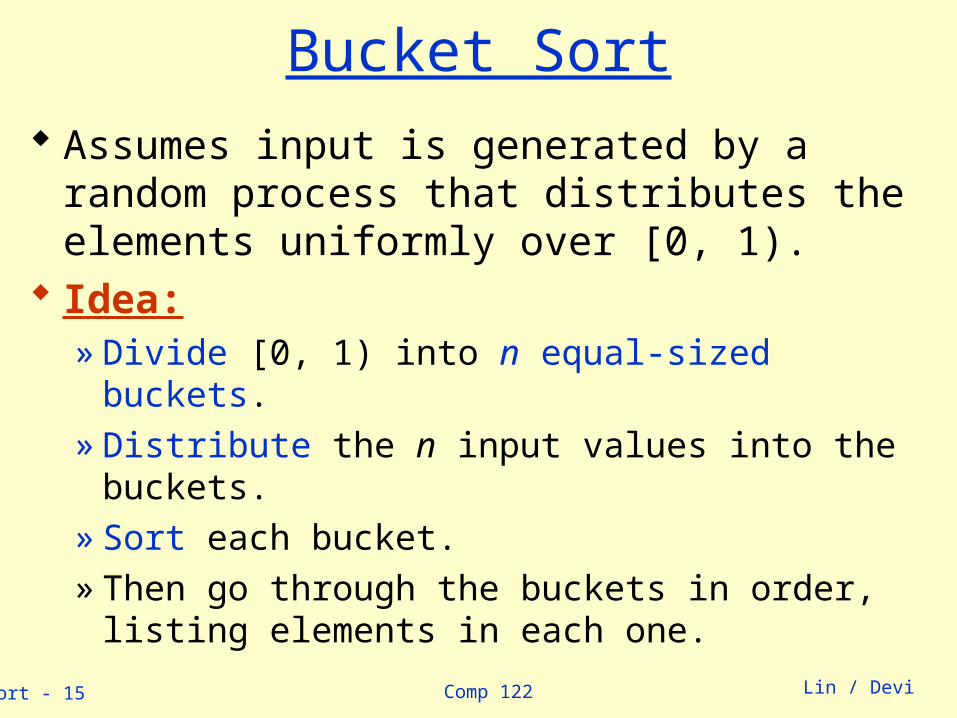
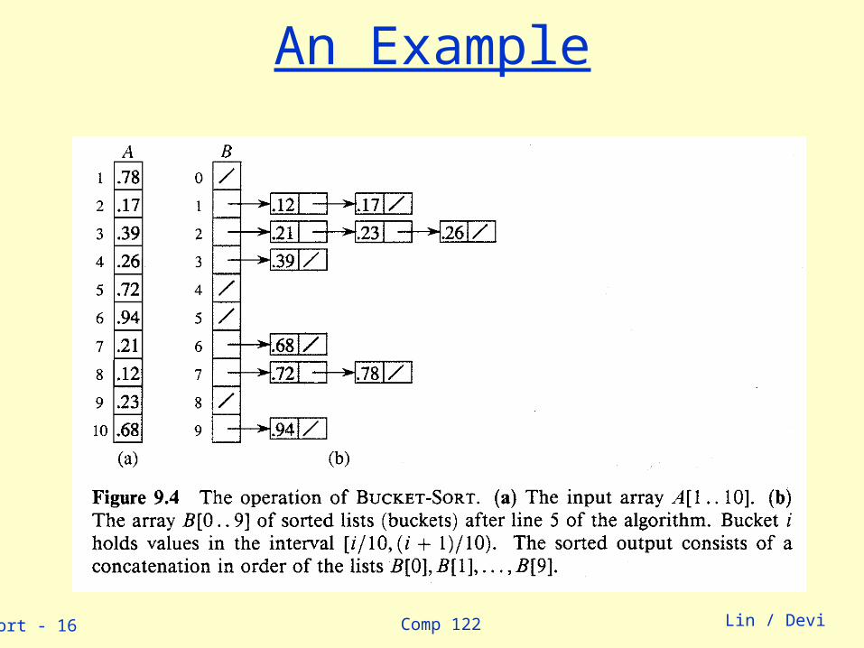
Assumes input is generated by a random process that distributes the elements uniformly over [0, 1).

Idea:» Divide [0, 1) into n equal-sized buckets.» Distribute the n input values into the buckets.» Sort each bucket.» Then go through the buckets in order, listing elements

in each one.


An Example


Bucket-Sort (A)

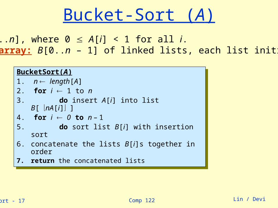
BucketSort(A)1. n length[A]2. for i 1 to n3. do insert A[i] into list B[ nA[i] ]4. for i 0 to n – 1 5. do sort list B[i] with insertion sort6. concatenate the lists B[i]s together in order7. return the concatenated lists

BucketSort(A)1. n length[A]2. for i 1 to n3. do insert A[i] into list B[ nA[i] ]4. for i 0 to n – 1 5. do sort list B[i] with insertion sort6. concatenate the lists B[i]s together in order7. return the concatenated lists

Input: A[1..n], where 0 A[i] < 1 for all i.Auxiliary array: B[0..n – 1] of linked lists, each list initially empty.


Analysis

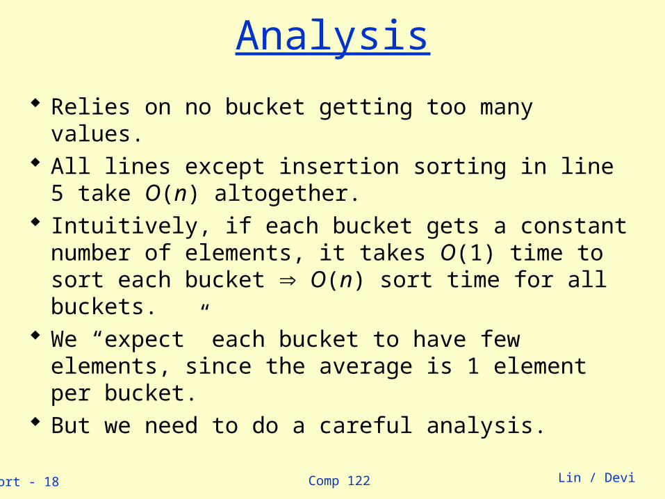
Relies on no bucket getting too many values. All lines except insertion sorting in line 5 take O(n)

altogether. Intuitively, if each bucket gets a constant number of

elements, it takes O(1) time to sort each bucket O(n) sort time for all buckets.

We “expect” each bucket to have few elements, since the average is 1 element per bucket.

But we need to do a careful analysis.


Analysis – Contd.

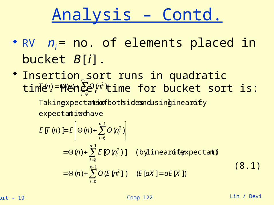
RV ni = no. of elements placed in bucket B[i]. Insertion sort runs in quadratic time. Hence, time for

bucket sort is:

1

0

2

1

0

2

1

0

2

1

0

2

)][][( ])[()(

n)expectatio oflinearity (by )]([)(

)()()]([

have wen,expectatio

oflinearity using and sidesboth of nsexpectatio Taking

)()()(

n

ii

n

ii

n

ii

n

ii

XaEaXEnEOn

nOEn

nOnEnTE

nOnnT

(8.1)


Analysis – Contd.

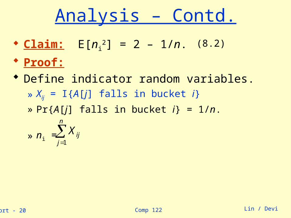
Claim: E[ni2] = 2 – 1/n.

Proof: Define indicator random variables.

» Xij = I{A[j] falls in bucket i}

» Pr{A[j] falls in bucket i} = 1/n.

» ni =

n

jijX

1

(8.2)


Analysis – Contd.

njkj

nkikij

n

jij

n

j njkj

nkikijij

ik

n

j

n

kij

n

jiji

XXEXE

XXX

XXE

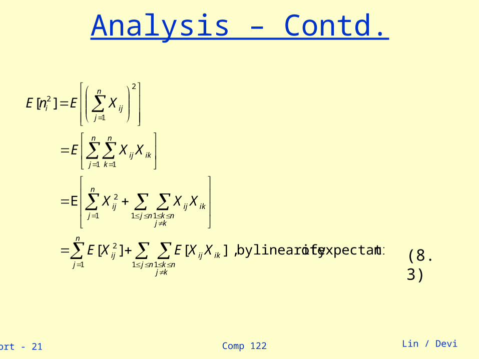
XEnE

1 11

2

1 1 1

2

1 1

2

1

2

n.expectatio oflinearity by , ][][

E

][

(8.3)


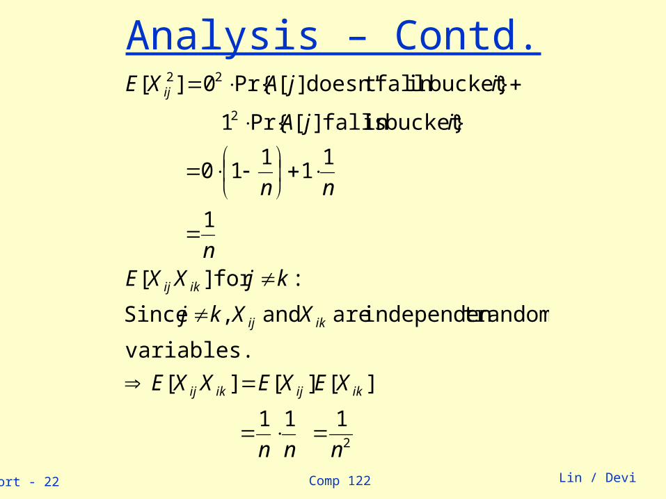
Analysis – Contd.

2

2

22

1

11

][][][

variables.

randomt independen are and , Since

:for ][

1

11

110

}bucket in falls ][Pr{1

}bucket in fallt doesn' ][Pr{0][

nnn

XEXEXXE

XXkj

kjXXEn

nn

ijA

ijAXE

ikijikij

ikij

ikij

ij


Analysis – Contd.

)(

)()(

)/12()()]([

.1

2

11

1)1(

1

11][

1

0

2

1 1 12

2

n

nOn

nOnnTE

n

nn

nnn

nn

nnnE

n

i

n

j njjk

nki

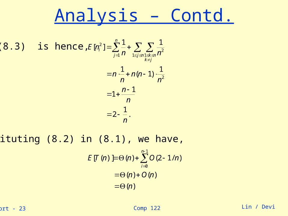
Substituting (8.2) in (8.1), we have,

(8.3) is hence,

Comp 122, Spring 2004

Hash Tables – 1Hash Tables – 1


Dictionary Dictionary:

» Dynamic-set data structure for storing items indexed using keys.

» Supports operations Insert, Search, and Delete.» Applications:

• Symbol table of a compiler.• Memory-management tables in operating systems. • Large-scale distributed systems.

Hash Tables:» Effective way of implementing dictionaries.» Generalization of ordinary arrays.


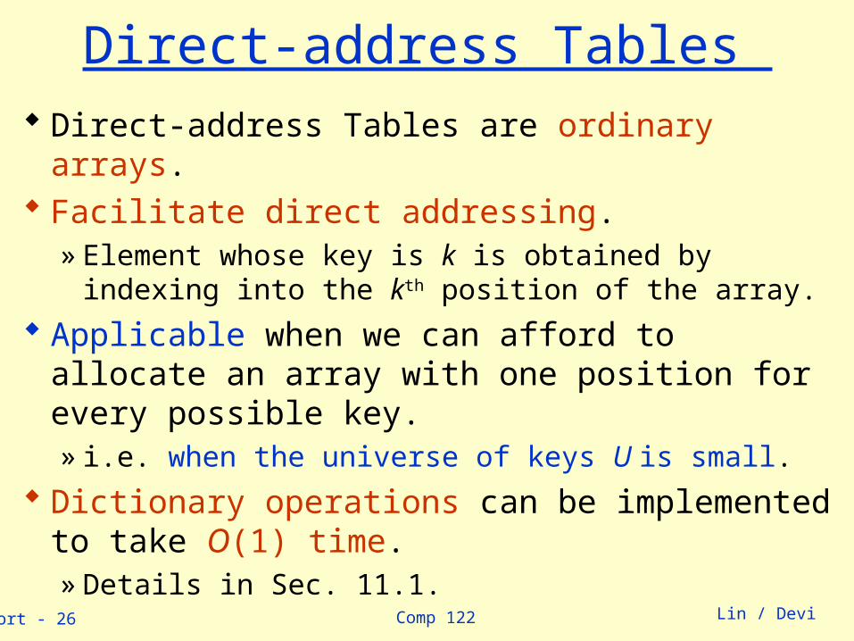
Direct-address Tables Direct-address Tables are ordinary arrays. Facilitate direct addressing.

» Element whose key is k is obtained by indexing into the kth position of the array.

Applicable when we can afford to allocate an array with one position for every possible key.» i.e. when the universe of keys U is small.

Dictionary operations can be implemented to take O(1) time.» Details in Sec. 11.1.


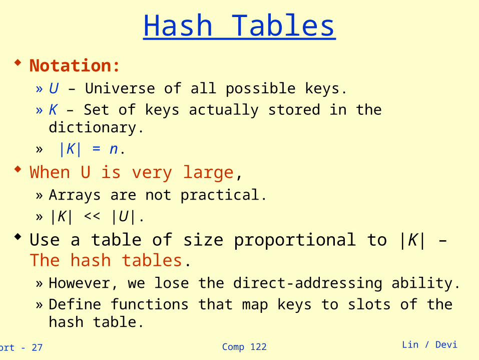
Hash Tables Notation:

» U – Universe of all possible keys.

» K – Set of keys actually stored in the dictionary.

» |K| = n.

When U is very large,» Arrays are not practical.

» |K| << |U|.

Use a table of size proportional to |K| – The hash tables.» However, we lose the direct-addressing ability.

» Define functions that map keys to slots of the hash table.


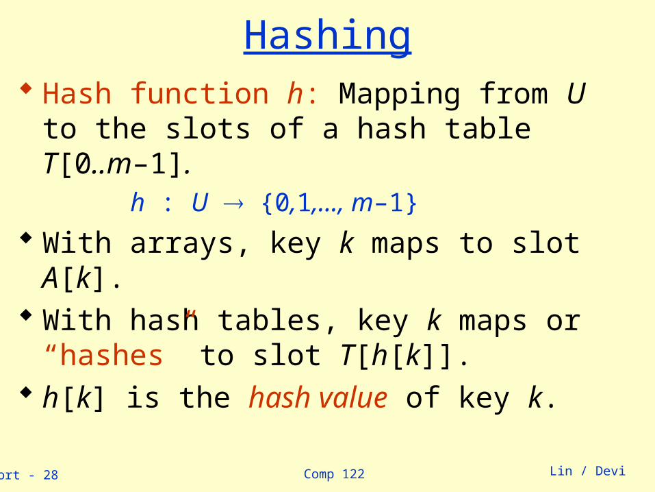
Hashing Hash function h: Mapping from U to the slots of a

hash table T[0..m–1]. h : U {0,1,…, m–1}

With arrays, key k maps to slot A[k].With hash tables, key k maps or “hashes” to slot

T[h[k]]. h[k] is the hash value of key k.


Hashing

0

m–1

h(k1)

h(k4)

h(k2)=h(k5)

h(k3)

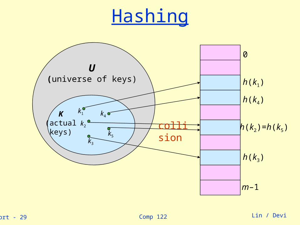
U(universe of keys)

K(actualkeys)

k1

k2

k3

k5

k4

collision


Issues with HashingMultiple keys can hash to the same slot –

collisions are possible.» Design hash functions such that collisions are

minimized.» But avoiding collisions is impossible.

• Design collision-resolution techniques.

Search will cost Ө(n) time in the worst case.» However, all operations can be made to have an

expected complexity of Ө(1).


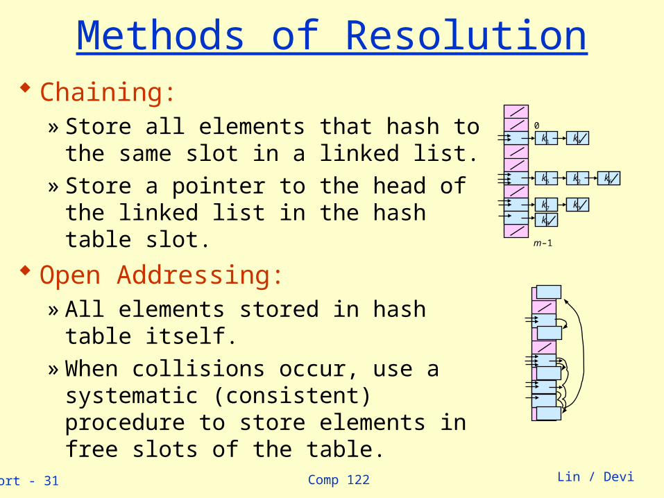
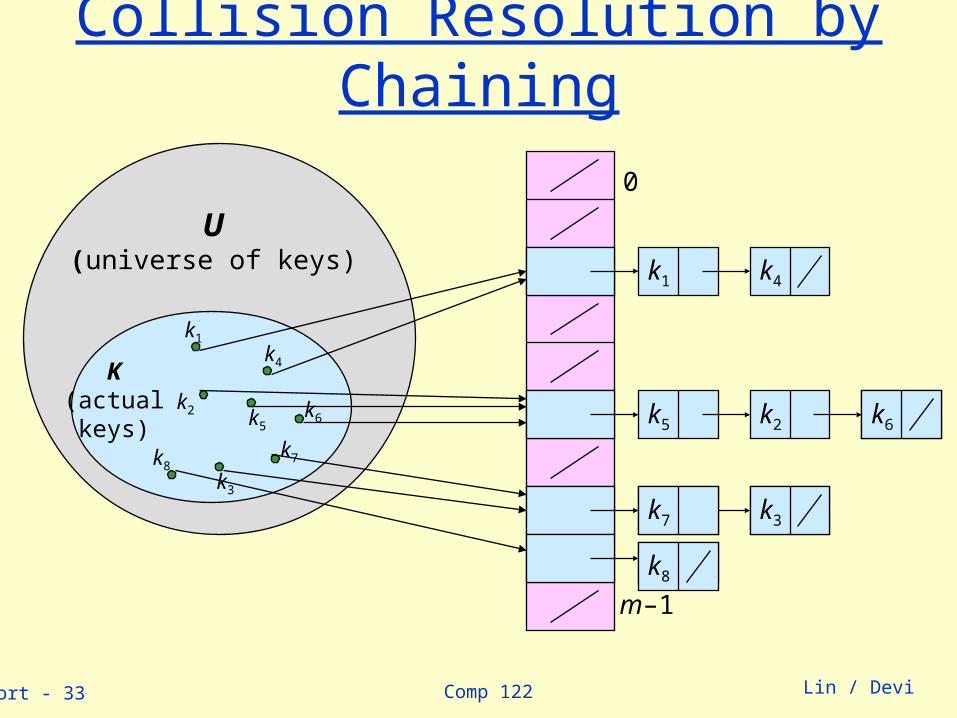
Methods of Resolution Chaining:

» Store all elements that hash to the same slot in a linked list.

» Store a pointer to the head of the linked list in the hash table slot.

Open Addressing:» All elements stored in hash table itself.» When collisions occur, use a systematic

(consistent) procedure to store elements in free slots of the table.

k2

0

m–1

k1 k4

k5 k6

k7 k3

k8


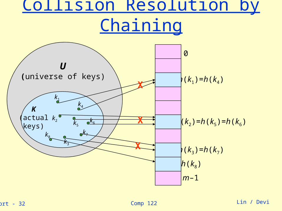
Collision Resolution by Chaining

0

m–1

h(k1)=h(k4)

h(k2)=h(k5)=h(k6)

h(k3)=h(k7)

U(universe of keys)

K(actualkeys)

k1

k2

k3

k5

k4

k6

k7k8

h(k8)

X

X

X


k2

Collision Resolution by Chaining

0

m–1

U(universe of keys)

K(actualkeys)

k1

k2

k3

k5

k4

k6

k7k8

k1 k4

k5 k6

k7 k3

k8


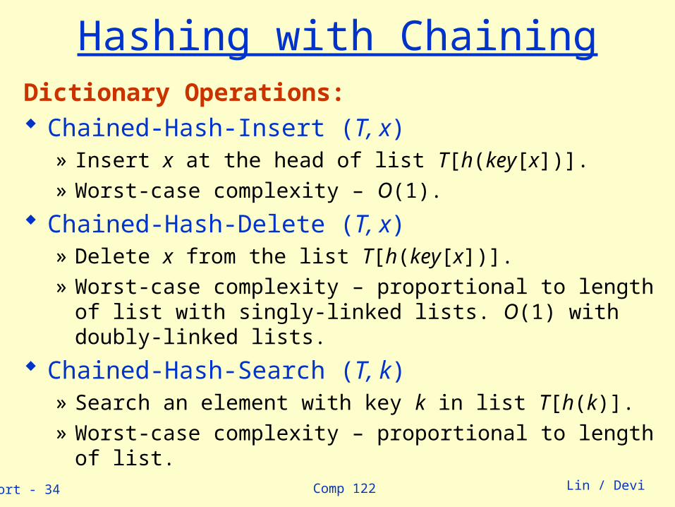
Hashing with ChainingDictionary Operations: Chained-Hash-Insert (T, x)

» Insert x at the head of list T[h(key[x])].

» Worst-case complexity – O(1).

Chained-Hash-Delete (T, x)» Delete x from the list T[h(key[x])].

» Worst-case complexity – proportional to length of list with singly-linked lists. O(1) with doubly-linked lists.

Chained-Hash-Search (T, k)» Search an element with key k in list T[h(k)].

» Worst-case complexity – proportional to length of list.


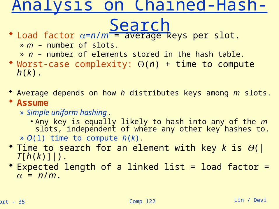
Analysis on Chained-Hash-Search Load factor =n/m = average keys per slot.

» m – number of slots.» n – number of elements stored in the hash table.

Worst-case complexity: (n) + time to compute h(k).

Average depends on how h distributes keys among m slots. Assume

» Simple uniform hashing.• Any key is equally likely to hash into any of the m slots,

independent of where any other key hashes to.» O(1) time to compute h(k).

Time to search for an element with key k is (|T[h(k)]|). Expected length of a linked list = load factor = = n/m.


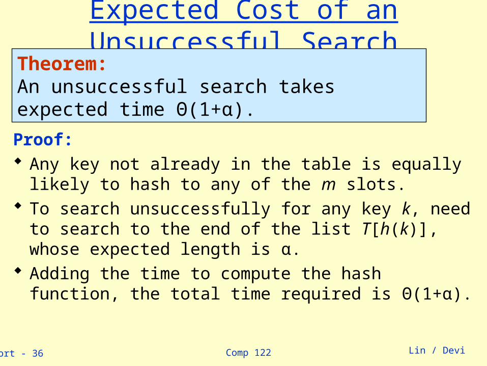
Expected Cost of an Unsuccessful Search

Proof: Any key not already in the table is equally likely to hash

to any of the m slots. To search unsuccessfully for any key k, need to search to

the end of the list T[h(k)], whose expected length is α. Adding the time to compute the hash function, the total

time required is Θ(1+α).

Theorem:An unsuccessful search takes expected time Θ(1+α).


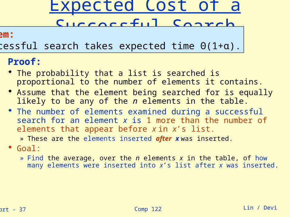
Expected Cost of a Successful Search

Proof: The probability that a list is searched is proportional to the number of

elements it contains. Assume that the element being searched for is equally likely to be any of

the n elements in the table. The number of elements examined during a successful search for an

element x is 1 more than the number of elements that appear before x in x’s list.» These are the elements inserted after x was inserted.

Goal:» Find the average, over the n elements x in the table, of how many elements were

inserted into x’s list after x was inserted.

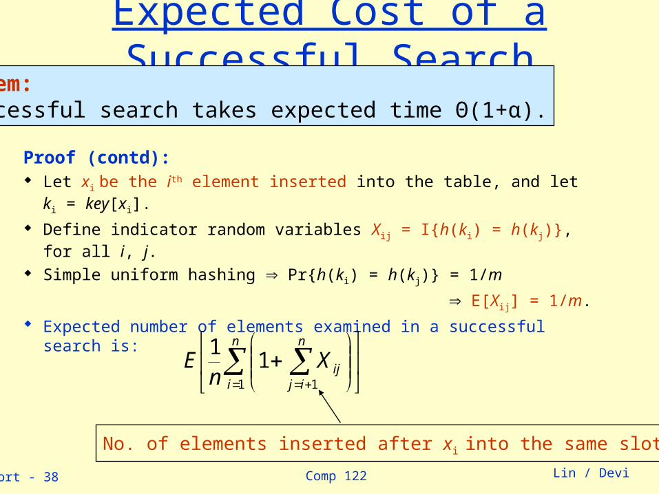
Theorem:A successful search takes expected time Θ(1+α).


Expected Cost of a Successful Search

Proof (contd): Let xi be the ith element inserted into the table, and let ki = key[xi].

Define indicator random variables Xij = I{h(ki) = h(kj)}, for all i, j.

Simple uniform hashing Pr{h(ki) = h(kj)} = 1/m

E[Xij] = 1/m.

Expected number of elements examined in a successful search is:

Theorem:A successful search takes expected time Θ(1+α).

n

i

n

ijijX

nE

1 1

11

No. of elements inserted after xi into the same slot as xi.


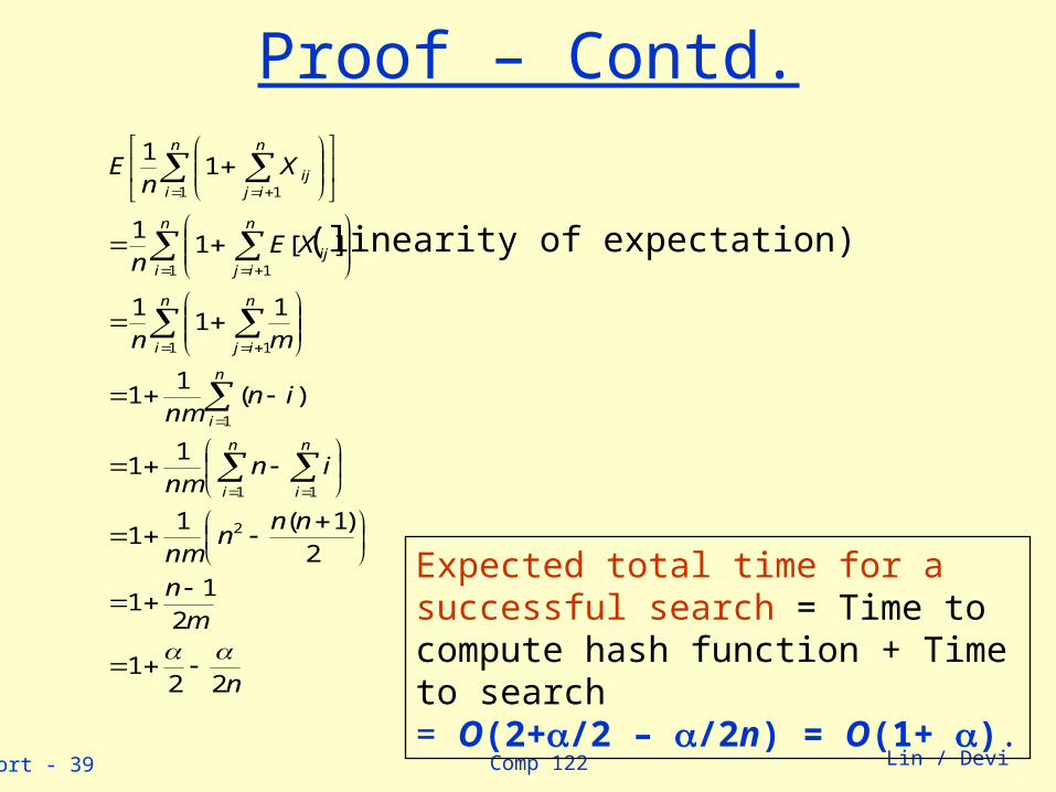
Proof – Contd.

n

mn

nnn

nm

innm

innm

mn

XEn

Xn

E

n

i

n

i

n

i

n

i

n

ij

n

i

n

ijij

n

i

n

ijij

221

21

1

2)1(1

1

11

)(1

1

11

1

][11

11

2

1 1

1

1 1

1 1

1 1

(linearity of expectation)

Expected total time for a successful search = Time to compute hash function + Time to search= O(2+/2 – /2n) = O(1+ ).


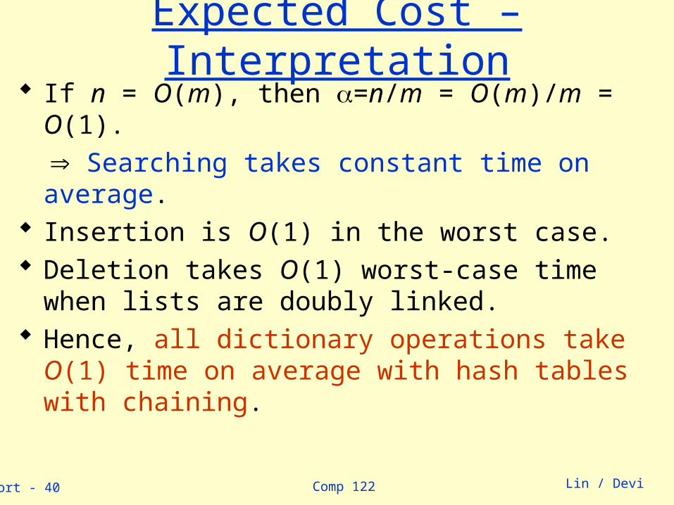
Expected Cost – Interpretation If n = O(m), then =n/m = O(m)/m = O(1).

Searching takes constant time on average. Insertion is O(1) in the worst case. Deletion takes O(1) worst-case time when lists are doubly

linked. Hence, all dictionary operations take O(1) time on

average with hash tables with chaining.

comp 122, spring 2004 keys into buckets: lower bounds, linear-time sort, & hashing

Documents

lower bound of n lg

n lg n merge sort

n lg n comparisons

comparison sort algorithm

values n

n lg n qed theorem

insertion sort

radix sort