COMP 290 – Data Mining Final Project Using sequence mining techniques for performance data

Todd Gamblin

Abstract For this project, we attempted to evaluate the effectiveness of rudimentary sequence mining techniques for characterizing I/O trace data. We have taken trace information for a scientific application running on a cluster, and we have attempted to use K-Medoids based clustering algorithms to correlate particular trace sequences with phases of application execution. We also present a novel approach to sequence comparison, where we consider packets in sequences qualitatively based on high-level observations about the distribution of their durations. We show that our approach can reveal correlations between I/O sequences and phases of application execution, and that sequence mining techniques hold promise for adaptive performance monitoring. 1. Introduction and Motivation With the advent of Grid Computing, an application designer may never know the exact performance characteristics of the environment in which his application runs. An application may run on a set of nodes that have completely different memory systems, disk drives, and associated resources, and it is thus the responsibility of the runtime system to discover these details and optimize the behavior of an application accordingly. To do this, it must be possible to detect, for a particular application, what phase of execution it is in at a particular time, based only on performance data collected from the running system. This information can then be used to guide the way the nodes the application is running on are monitored, and to dynamically assign resources to the application to improve its performance. Large cluster systems today can have thousands of nodes, and monitoring all of them in real-time is beyond the capabilities of current interconnection networks. Statistical sampling can be used to significantly reduce the number of nodes we need to monitor and, accordingly, the volume of data that needs to be sent over the network. In particular, if we establish a minimum acceptable accuracy for our results, we can determine a minimum sample size necessary to achieve that accuracy. This minimum sample size depends on the variability of the data. For data that varies less, it is possible to sample fewer nodes while maintaining the same accuracy. If we modulate the sample size

according to the variability of the data monitored, we can further reduce the load on the network. Since the performance characteristics of an application can vary by execution phase, and since execution phase in a dynamic application can vary by machine, we would like to be able to divide our nodes into different groups and sample each group independently. This could further reduce monitoring overhead. First, however, we need to understand what the different execution phases of applications are, and we need to learn how to identify them based on observable information. 2. Prior Work Hao Wang [9] has run tests on the same data we examine here, but his approach has did not consider the sequential nature of the data. Instead, he applied various data mining techniques to individual packets of data, without taking into account their order. Computer programs are inherently sequential, and their actions are difficult to characterize without examining their order. Streaming I/O references made by computer programs will also be strongly sequential, and mining for frequently occurring sequences of data will be more effective for characterization than analysis at the reference level. Lu and Reed [4] have investigated a low-overhead alternative to event tracing called “application signatures”. They use curve fitting to characterize individual performance metrics, and use these to compare applications across platforms. This technique is comparable to our sequence-mining approach, but our research is focused more on leveraging powerful existing data-mining techniques on available data than on low overhead. Much work has been done on sequential pattern matching (string matching) and on cluster mining in the past. Sequence mining and approximate string matching have had important applications to biological data, and we apply these techniques to performance data. In particular, we use the K-Medoids clustering algorithm [3], the CLARA [5] clustering algorithm, and the edit distance [7] measure of the similarity of sequences. 3. Data Characterization For this project, we ran tests on approximately 850 MB of application trace data from traces run by the University of Illinois Pablo project [6]. The data is in Pablo’s Self-Defining Data Format (SDDF), and it contains records of each I/O event that occurred during a particular run of Dyna3D [1], a structural mechanics simulator. The simulation we examine ran on 32 nodes of the ASCI Blue system (blue.pacific.llnl.gov), and the dataset was a physical model containing 1,046,797 nodal points. Dyna3D performance can be very data dependent, so it will be especially beneficial for us to identify different phases in its execution, as we may be able to perform load-balancing between nodes, or reallocate resources based on this kind of information.

The fundamental unit of data in an SDDF file is called a “packet”. Some of these represent I/O trace events, while others are actual I/O system calls made by the application. There are 9,594,415 packets total. For the purpose of this project, we have filtered out the trace events, since it is only the system calls that we would be monitoring in an actual runtime environment. A packet relevant to us in the data might look like this: "Write" {

[2] { -382203,1}, 214.738809725, 700017, 15, 0.0032184, 38, 13, 0, 0

};; Each packet has a type name, specified on its first line. The six specific types of packets we are concerned with are Read, Write, Open, Close, Seek, and Flush. These are the names of well-known I/O operations, so we will not explain them in detail here. The second line of the packet is its timestamp in two forms: the first is an array of ints, and the second is the same value represented as a double. The third line contains the following fields:

1. Unique id of the packet 2. Id of the node on which the I/O operation occurred 3. Duration of the operation in seconds 4. Id of the file the operation refers to, 5. Number of bytes read/written by the operation 6. Number of variables passed to the I/O call 7. Bookkeeping value used by the instrumentation code that recorded this data

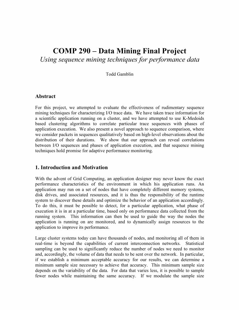
The timestamp field is important for our analysis, because events with similar timestamps can represent the same phase of application execution. If we can show correlations between other attributes and time, then we may be able to use this kind of data to learn about running applications. Number of bytes, number of variables passed to the I/O call, and the duration of the I/O operation might also be of concern at runtime. Before we started writing our code, we looked at the distribution of these values across the data. Our results are presented below.

Figure 1: Histogram of Operation Types

The data is consists of 9,138,950 reads, 449,431 writes, 256 file opens, 227 closes, and 31 seeks. There are no flushes, and there are a total of 9,588,895 operations.

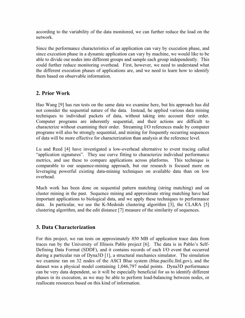
Figure 2: Histogam of values for bytes read/written in I/O Operations

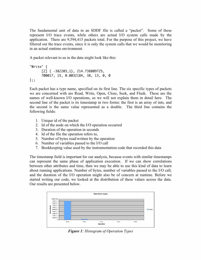
There were very few values for the number of bytes read or the number of bytes written in I/O operations. Either 1 or 18 bytes were read at a time, and 2, 4, 13, or 15 were written at a time. The number of variables passed to read calls, along with the number of variables passed to write calls, was always zero in the data we used, so there was no information to be gained from this dimension of the data. The duration of I/O operations was the most varied metric for the I/O references we examined. The distributions of values for Each type of I/O operation are shown below.

Figure 3: Durations of reads and writes.

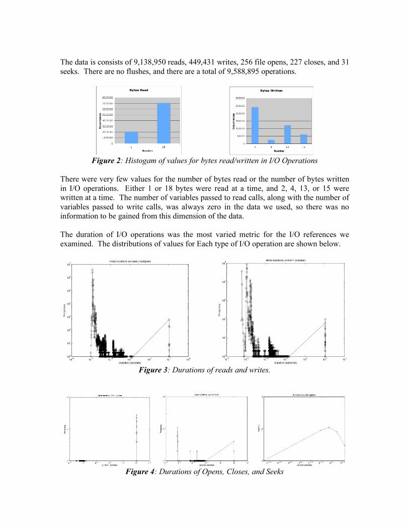
Figure 4: Durations of Opens, Closes, and Seeks

A large number of read operations are tightly grouped around 10-6

seconds, while smaller groups of reads tend to take around 10-4 seconds. There are almost no reads taking more than 10-2 seconds, save for a small group taking around 100 seconds to complete. Writes vary in a similar fashion to the reads. The largest portion of writes is around 10-6 seconds in duration, tapering off to close to zero writes above 10-2 seconds Just as with the reads, there is a small group of writes taking around 100 seconds to complete. The speed of reads and writes in the system can be related to the memory hierarchy of the system tested, or it could be related to the virtual memory system of the machine. Slower times could imply a cache miss or a page fault, or a higher load on the machine on which these timings were observed. They can tell us important information about the performance of the application at the point in time they were observed. The duration data thus seems to be the most relevant for our mining algorithms. Other operations are far less frequent than writes or reads are in the dataset. Closes seem to follow a similar distribution to the writes and the reads, while seeks are all in the 10-6 second range. The distribution of opens is similar to reads, writes, and closes, but without the large number of fast operations that we see with these other types. 4. Adapting algorithms for analysis of performance data In this section, we describe how we have adapted existing algorithms for approximate string comparison and for data mining to work with our performance data. We present a novel high-level way of looking at sequences, where we categorize reads and writes into bins based on their distribution as described in Section 3, and we then describe how sequences of this sort can be used as input for clustering algorithms. 4.1. Mapping Q-Grams to I/O Traces String matching is typically defined in terms of characters in sequence, or, in the case of genetics, in terms of bases in DNA molecules. We will be using packets as characters, and sequences, called q-grams [8], of them in place of strings. Q-grams are discussed in [8,9], and the term generally refers to taking a stream of inputs and breaking it into subsequences of a fixed length, q. In our case, we do just that: we split the data stream into q-grams of packets. As q-grams are sequential, comparing them instead of individual packets should give us more of a sense for the types of tasks the application is performing, rather than for the overall mix of operations it is using. To compare q-grams with each other, we need some definition of what makes two packets equal. We obviously cannot compare two packets for equality based on their timestamps, as this would result in none of them being equal. Instead, we define three different measures for packet equality based on the attributes available to us in the data, and we look for the q-grams that met these criteria.

1. Operation-Type equality If two packets have the same operation type, they are considered equal.

2. Exact duration equality

If two packets are of the same type, and they have the exact same duration, they are considered to be equal.

3. Binned duration equality

Similar to operation type equality, but with slightly finer granularity. Since the duration values for read and write are so varied, we chose to group them in bins. Reads slower than 10-5 seconds are considered “short reads”, those longer than 1 second are considered “long reads”, and those in between are considered “middle reads”. Writes are handled similarly.

Two q-grams are considered equal if all of their component packets are equal. We use a trie data structure to search for the unique q-grams in our data, and we test this with each of the above definitions of equality. 4.2. Clustering Q-Grams Clustering is a technique widely used in data mining to find groups of similar objects within a larger dataset. The frequent q-gram search we described above can find frequently occurring q-grams, but it will find only exact sequence matches. We wanted to find equivalence classes of similar q-grams in the data. Given these, we could characterize data at runtime based on its membership in these classes, and we could use this information to deduce how an application is running. Clustering data requires some means for assessing how points are similar. In our case, our points are q-grams, and we can again look to string matching research. A common measure of the dissimilarity of sequential strings is the edit distance. Edit distance is a measure of how many changes (e.g. adding, deleting, or replacing characters) would need to be made to make one string into another. Given two q-grams, we can again treat packets as characters, and using the equality measures outlined above we can calculate the edit distance between two q-grams. Our clustering algorithms use this as their measure of q-gram similarity. Traditional methods for clustering include K-Means [3], K-Medoids[3], and Density Clustering [2]. K-Means and K-Medoids are similar in that they both attempt to create a fixed number of clusters, k, by assigning clusters and minimizing the total dissimilarity of points within them. K-Means tries to minimize the sum of square dissimilarities of points in a cluster from their mean value. K-Medoids uses medoids instead of means, where a medoid is restricted to being an actual point in a cluster rather than the average of the positions of all points. Density-based clustering algorithms take a different approach, and try to find groups of points that are “density connected,” without considering overall dissimilarity. This tends to be a more robust method than the K-cluster based

approaches, as it can find clusters with arbitrary shape. Also, Density Clustering does not need to know the number of clusters to search for in advance. Of these methods, the only one applicable to our sequence data is K-Medoids. Because the only two operations we have defined on our q-grams are equality and edit distance, we cannot use K-Means or Density Clustering. K-Means requires the computation of a mean from the data points, but all we have is a measure of dissimilarity. There is no way to compute a “mean” q-gram. Density clustering suffers from similar problems, and is only applicable to spatial data. K-Medoids, however, can be applied, as it only requires a measure of “distance” between two points to be applicable. A proper distance measure must obey the triangle inequality, that is, for any three points x, y, and z, the distance d(x,y) ≤ d(x,z) + d(z,y). The edit distance does obey this property, and it is thus usable for K-Medoids clustering. K-Medoids is the slowest of the above mentioned clustering algorithms, and it is not practical for large datasets. A single iteration of K-Medoids requires O(k(n-k)2) time. Running sufficient iterations of this algorithm for a large dataset to converge could take an unmanageable amount of time. Therefore, we chose to use CLARA [5], which offers significantly better performance. Instead of clustering an entire dataset, CLARA samples the dataset several times and runs K-Medoids on the sample. It then chooses from the sample runs the best set of medoids for the total dataset. CLARA has been shown to perform well on large datasets like ours. It is worth noting that the sequence clustering problem has been looked at in considerable detail by Wang, et al. They presented CLUSEQ, an algorithm for finding clusters in sequential data without a preset number of clusters to find, and without a preset length of sequences to cluster on (as our q-gram analysis inherently requires). Also, CLUSEQ measures similarity by statistical properties of sequences, rather than on a single distance metric. We believe that this algorithm would be very effective in analyzing I/O trace data, but it was not available at the time we performed our experiments. The algorithm is very sophisticated, and there was not time available to rewrite and then debug it. We believe that testing CLUSEQ holds promise for testing performance data in the future. 4.3. Implementation We have implemented all of the above algorithms in C++. Our implementation uses the Pablo project’s library for processing SDDF data as its backend. It first reads sequence data from SDDF files, splits it into q-grams, and stores unique q-grams in a trie. The trie is then queried for frequent q-grams. We then pass these q-grams on to the CLARA clustering algorithm. We then relate each of these unique q-grams to all instances of them in the main dataset to calculate statistics for the clusters.

5. Q-Gram Results In this section, we describe the experiments we performed and the results we obtained from applying our q-gram and cluster algorithms to the Dyna3D dataset. 5.1 Unique Q-Grams Our first experiment was to count the number of unique q-grams in the dataset. We show that the number of unique q-grams in an I/O trace can give us an idea of the variety and relative complexity of behavior in the system. We first ran q-gram on our raw dataset, with I/O trace packets from the different nodes interleaved in the order they were traced. We then split the data into separate files, one per node, and ran the same experiment on the split data. We compared the results with the number of unique q-grams in the un-split data set. Finally, we looked at the distribution of all instances of these unique q-grams in time, to see if there was any temporal locality among like q-grams.

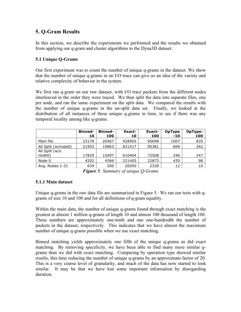
Figure 5: Summary of unique Q-Grams 5.1.1 Main dataset Unique q-grams in the raw data file are summarized in Figure 5. We ran our tests with q-grams of size 10 and 100 and for all definitions of q-gram equality. Within the main data, the number of unique q-grams found through exact matching is the greatest at almost 1 million q-grams of length 10 and almost 100 thousand of length 100. These numbers are approximately one-tenth and one one-hundredth the number of packets in the dataset, respectively. This indicates that we have almost the maximum number of unique q-grams possible when we use exact matching. Binned matching yields approximately one fifth of the unique q-grams as did exact matching. By removing specificity, we have been able to find many more similar q-grams than we did with exact matching. Comparing by operation type showed similar results, this time reducing the number of unique q-grams by an approximate factor of 20. This is a very coarse level of granularity, and much of the data has now started to look similar. It may be that we have lost some important information by disregarding duration.

Binned-

10 Binned-

100 Exact-

10 Exact-

100 OpType

-10 OpType-

100

Main file 23178 20467 928905 95698 1007 835

All Split (w/node0) 21903 19863 831517 95381 669 342 All Split (w/o node0) 17829 15497 610464 72508 246 247

Node 0 4202 4366 221405 22873 430 98 Avg. Nodes 1-31 634 500 20050 2339 12 10

Node

Binned- 10

Binned-100

Exact-10

Exact-100

Type-10

Type-100

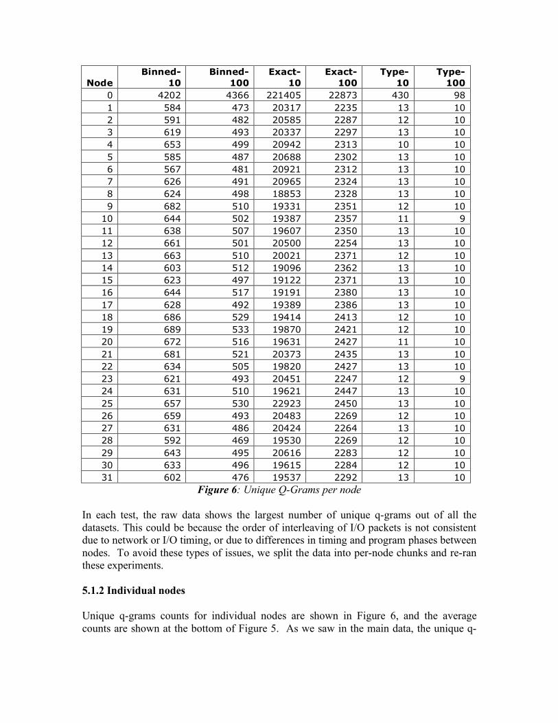
0 4202 4366 221405 22873 430 98 1 584 473 20317 2235 13 10 2 591 482 20585 2287 12 10 3 619 493 20337 2297 13 10 4 653 499 20942 2313 10 10 5 585 487 20688 2302 13 10 6 567 481 20921 2312 13 10 7 626 491 20965 2324 13 10 8 624 498 18853 2328 13 10 9 682 510 19331 2351 12 10

10 644 502 19387 2357 11 9 11 638 507 19607 2350 13 10 12 661 501 20500 2254 13 10 13 663 510 20021 2371 12 10 14 603 512 19096 2362 13 10 15 623 497 19122 2371 13 10 16 644 517 19191 2380 13 10 17 628 492 19389 2386 13 10 18 686 529 19414 2413 12 10 19 689 533 19870 2421 12 10 20 672 516 19631 2427 11 10 21 681 521 20373 2435 13 10 22 634 505 19820 2427 13 10 23 621 493 20451 2247 12 9 24 631 510 19621 2447 13 10 25 657 530 22923 2450 13 10 26 659 493 20483 2269 12 10 27 631 486 20424 2264 13 10 28 592 469 19530 2269 12 10 29 643 495 20616 2283 12 10 30 633 496 19615 2284 12 10 31 602 476 19537 2292 13 10

Figure 6: Unique Q-Grams per node In each test, the raw data shows the largest number of unique q-grams out of all the datasets. This could be because the order of interleaving of I/O packets is not consistent due to network or I/O timing, or due to differences in timing and program phases between nodes. To avoid these types of issues, we split the data into per-node chunks and re-ran these experiments. 5.1.2 Individual nodes Unique q-grams counts for individual nodes are shown in Figure 6, and the average counts are shown at the bottom of Figure 5. As we saw in the main data, the unique q-

gram count is greatest when we do exact matching on the duration of operations, one-fifth that size for binned matching, and much smaller if we match on type of operation. There are two things of note about the data in Figure 6. First, the unique q-gram count for Node 0 is far more than for that of any other node. This indicates that Node 0’s I/O behavior is more varied than that of the other nodes. We can assume that Node 0 is doing more varied computation than the others. Given that Dyna3D is an MPI application, we could postulate that Node 0 is a control node, doling out computational tasks the other nodes. The second interesting property of the data in Figure 6 is that the number of unique q-grams for nodes 1-31 is relatively consistent in all cases. The number hovers around 600 for binned q-grams of length 10 and around 500 for binned q-grams of length 100. For operation type q-grams, the count is around 10 or 12. The exact q-gram count stays around 20,000. It is important to note that this number, like the raw data q-gram count for the main dataset, is almost the count of all unique q-grams per node. This tells us there are few similarities between q-grams in the same node, but it does not tell us how many of these unique are similar to q-grams in other nodes. 5.1.2 Individual nodes combined To determine if there were similarities between unique q-grams on different nodes, we took our split node data and searched for unique q-grams over the entire data set. Our results for this experiment are shown in Figure 5 as “All Split”. Since node 0 was shown to be markedly different, we did an additional run with its packets removed from the dataset, to see how similar nodes 1-31 were. We can see by comparing the split q-gram results to the results for Main that there are more shared q-grams in the entire dataset when the q-grams are split across nodes. There is a difference of approximately 2,000 q-grams between the main result and the all split result for binned q-grams of length 10, and a similar amount for length 100. Numbers of Operation Type q-grams were reduced even more significantly. Even the number of exact q-grams decreased when we split across nodes. Furthermore, when we remove node 0 from the mix, we can see that the datasets are even more similar. If we subtract the results without node 0 from the results with node 0, we see that node 0 accounts for about 1/5 of all unique q-grams in the split dataset, about ¼ in the exact dataset, and almost 2/3 of the operation type dataset. Shared q-grams between nodes indicate that the Dyna3D application nodes share certain phases of execution, and that we could use I/O traces to detect this. We substantiate this is section 5.2, where we discuss temporal distribution of the q-gram data.

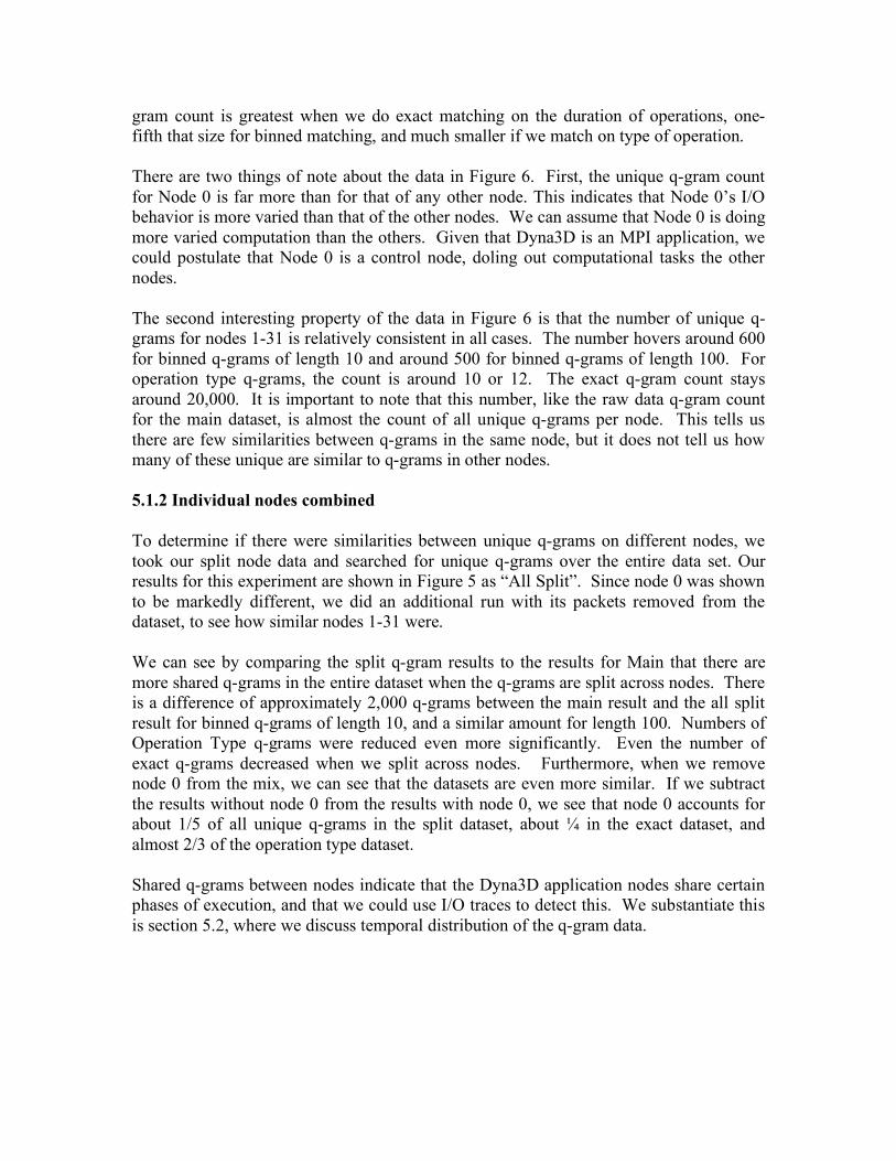
5.2 Temporal Locality of Unique Q-Grams For each unique q-gram in our datasets, we plotted the standard deviation of all times it occurred. We sorted the values so that it is easy to see qualitatively what portion of each dataset had what sort of standard deviation. The results are shown for q-grams of length 10 in Figure 7, and for q-grams of length 100 in Figure 8. The standard deviation in time of frequent q-grams should give us a sense for how much temporal locality is in the data set. A small standard deviation indicates that the q-grams occurred over a relatively small window in time, and a large one indicates that the particular q-gram may occur at many times during the Dyna3d run. 5.2.1 Main dataset In Figure 7 we show the results for the main dataset. For exact matching on 100 q-grams, the standard deviation for nearly the entire dataset was 0. This is because most q-grams in that dataset were unique. This is a case of too little temporal locality, as all the exact q-grams are occurring at different times. We may still be able to assign them to groups by clustering, but at first glance this is not promising. If we tried to use these q-grams for classifying runtime behavior, we would have to compare a monitored q-gram with a large portion of the dataset to determine what time it occurred. The standard deviation is higher for exact q-grams of length 10 and for the binned q-grams of length10 and 100. For all of these, most standard deviations fall between 10-3 and 10-4 seconds, with a small number of unique q-grams having deviations over a second. This means that shorter or binned q-grams are probably a better indicator for application behavior, and that we may be able to associate binned q-grams monitored at runtime with particular phases of application execution. For comparison by operation type, the standard deviation is slightly higher for q-grams of length10, and very large for nearly half the unique q-grams of length 100. A significant number of unique q-grams in both datasets have standard deviations of around 104 seconds. Note that this is the deviation for all occurrences of each unique q-gram, and that there tend to be more occurrences of q-grams with a large standard deviation. The total running time of this instance of Dyna3D was around 11,000 seconds, so we can see that most of the q-grams observed for length 100 and a smaller amount of those of length 10 occur at nearly every point in the dataset. This is not very useful, as we cannot take any one of these q-grams monitored at runtime and say with any certainty when it occurred.

Figure 7: Standard deviation in time of occurrences Q-Grams in the main, un-split

dataset. Results for q-grams of length 10 are shown at left, and for length 100 at right. The vertical axis shows standard deviation, while the horizontal axis shows unique q-

grams. Horizontal axes are normalized to the same range so we can compare datasets of different sizes. We are mainly interested in the percentage of q-grams in each dataset

with a particular standard deviation in time.

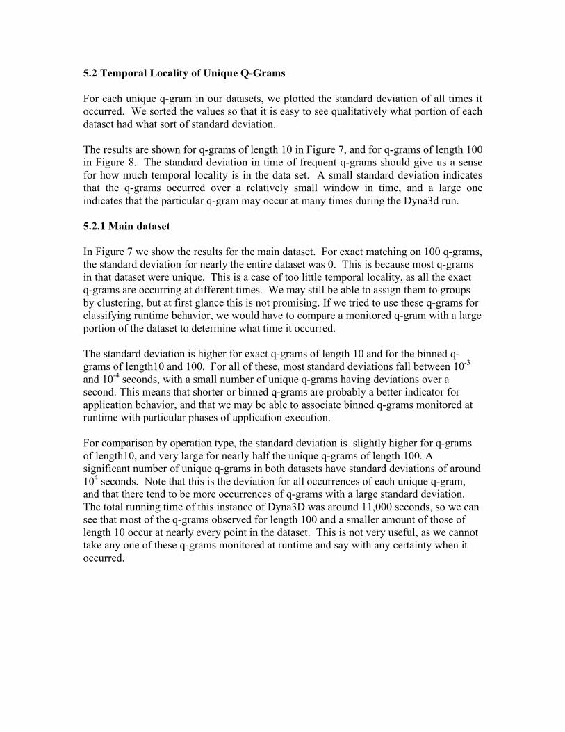
5.2.2 Individual Nodes Combined Figure 8 shows our results for the data split across nodes. We can see that again there are mostly unique q-grams of length 100 with exact matching. The standard deviation on all the other graphs, however, is much higher than it was without the nodes split. With binned q-grams in particular, the standard deviation is roughly an order of magnitude greater than it was in the raw dataset. This is because we have removed some noise by not considering the interleaving of packets across nodes, and we see that the dataset when split consists of fewer unique q-grams spanning over a longer amount of time. OpType q-grams look worse for the split dataset than they did for the main dataset. Taking out the noise of interleaving reveals more similarities between opType q-grams, to the point that nearly all of them occur over the entire dataset. This data would not be

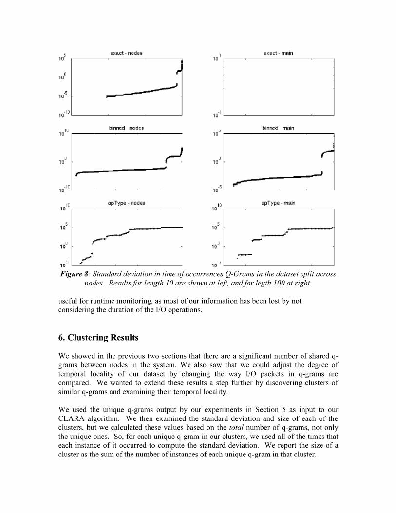
Figure 8: Standard deviation in time of occurrences Q-Grams in the dataset split across

nodes. Results for length 10 are shown at left, and for legth 100 at right. useful for runtime monitoring, as most of our information has been lost by not considering the duration of the I/O operations. 6. Clustering Results We showed in the previous two sections that there are a significant number of shared q-grams between nodes in the system. We also saw that we could adjust the degree of temporal locality of our dataset by changing the way I/O packets in q-grams are compared. We wanted to extend these results a step further by discovering clusters of similar q-grams and examining their temporal locality. We used the unique q-grams output by our experiments in Section 5 as input to our CLARA algorithm. We then examined the standard deviation and size of each of the clusters, but we calculated these values based on the total number of q-grams, not only the unique ones. So, for each unique q-gram in our clusters, we used all of the times that each instance of it occurred to compute the standard deviation. We report the size of a cluster as the sum of the number of instances of each unique q-gram in that cluster.

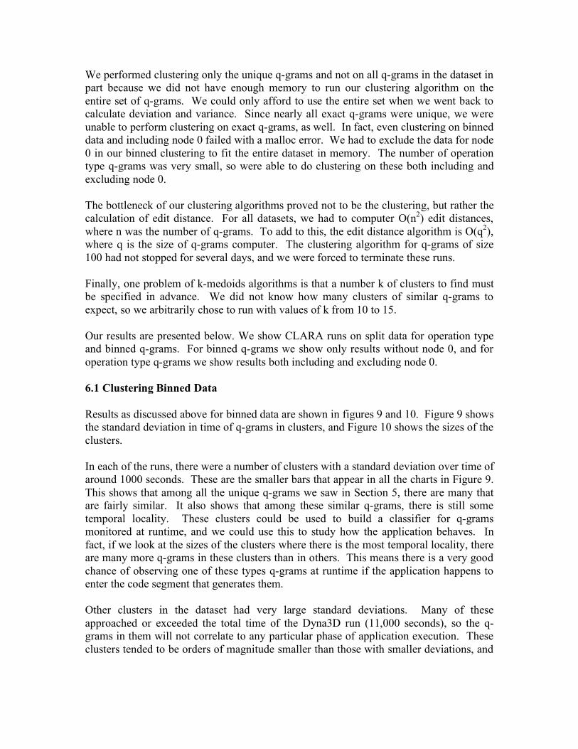
We performed clustering only the unique q-grams and not on all q-grams in the dataset in part because we did not have enough memory to run our clustering algorithm on the entire set of q-grams. We could only afford to use the entire set when we went back to calculate deviation and variance. Since nearly all exact q-grams were unique, we were unable to perform clustering on exact q-grams, as well. In fact, even clustering on binned data and including node 0 failed with a malloc error. We had to exclude the data for node 0 in our binned clustering to fit the entire dataset in memory. The number of operation type q-grams was very small, so were able to do clustering on these both including and excluding node 0. The bottleneck of our clustering algorithms proved not to be the clustering, but rather the calculation of edit distance. For all datasets, we had to computer O(n2) edit distances, where n was the number of q-grams. To add to this, the edit distance algorithm is O(q2), where q is the size of q-grams computer. The clustering algorithm for q-grams of size 100 had not stopped for several days, and we were forced to terminate these runs. Finally, one problem of k-medoids algorithms is that a number k of clusters to find must be specified in advance. We did not know how many clusters of similar q-grams to expect, so we arbitrarily chose to run with values of k from 10 to 15. Our results are presented below. We show CLARA runs on split data for operation type and binned q-grams. For binned q-grams we show only results without node 0, and for operation type q-grams we show results both including and excluding node 0. 6.1 Clustering Binned Data Results as discussed above for binned data are shown in figures 9 and 10. Figure 9 shows the standard deviation in time of q-grams in clusters, and Figure 10 shows the sizes of the clusters. In each of the runs, there were a number of clusters with a standard deviation over time of around 1000 seconds. These are the smaller bars that appear in all the charts in Figure 9. This shows that among all the unique q-grams we saw in Section 5, there are many that are fairly similar. It also shows that among these similar q-grams, there is still some temporal locality. These clusters could be used to build a classifier for q-grams monitored at runtime, and we could use this to study how the application behaves. In fact, if we look at the sizes of the clusters where there is the most temporal locality, there are many more q-grams in these clusters than in others. This means there is a very good chance of observing one of these types q-grams at runtime if the application happens to enter the code segment that generates them. Other clusters in the dataset had very large standard deviations. Many of these approached or exceeded the total time of the Dyna3D run (11,000 seconds), so the q-grams in them will not correlate to any particular phase of application execution. These clusters tended to be orders of magnitude smaller than those with smaller deviations, and

it is possible that they are simply clusters of outliers, or they could be an artifact of the fixed k-value not reflecting the actual number of significant clusters in the system.

Figure 9: Standard deviation of time for clusters of binned q-grams of length 10.

Y axis is time in seconds, and each bar represents a cluster.

Figure 10: Sizes of clusters binned q-grams of length 10. Y axis is number of q-grams.

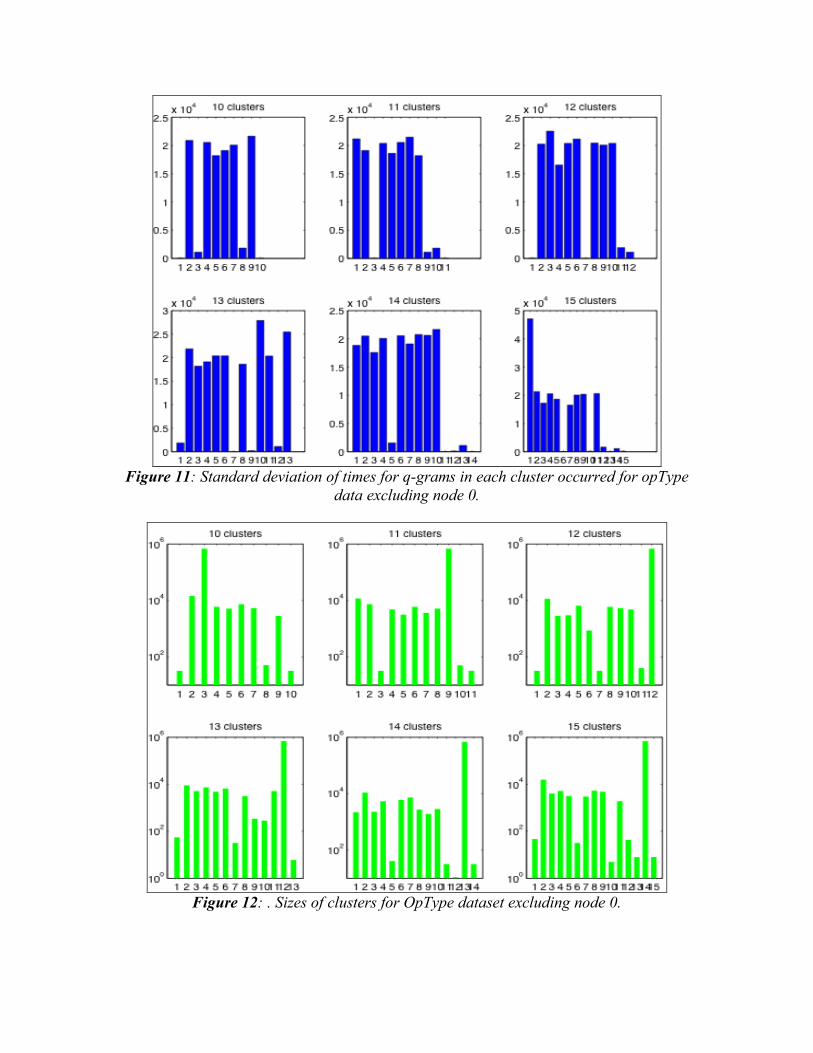
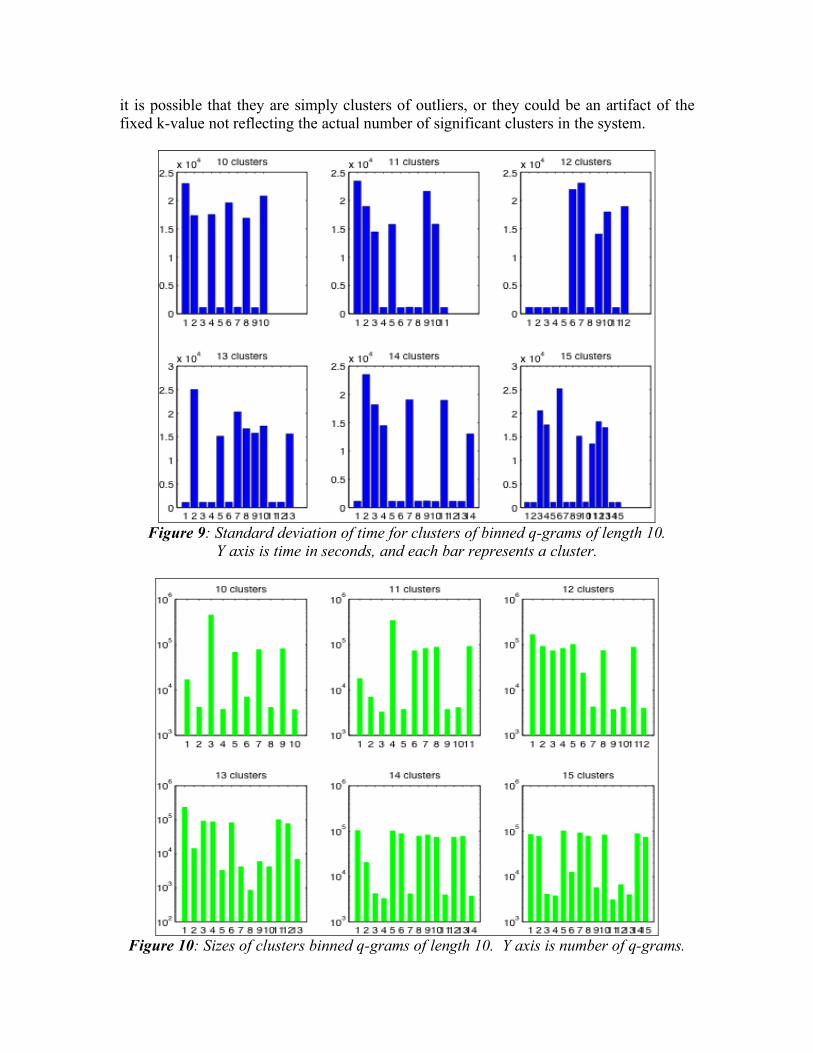
Figure 11: Standard deviation of times for q-grams in each cluster occurred for opType

data excluding node 0.

Figure 12: . Sizes of clusters for OpType dataset excluding node 0.

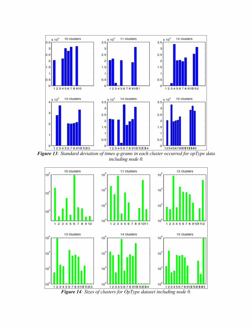
Figure 13: Standard deviation of times q-grams in each cluster occurred for opType data

including node 0.

Figure 14: Sizes of clusters for OpType dataset including node 0.

6.2 Clustering on OpType Data Standard deviations over time and cluster sizes for operation type clusters are shown in Figures 11-14. For the dataset with node 0 excluded (Figures 11 and 12), we see that there are some clusters in each run with a small standard deviation around 1000 seconds. This is similar to the binned datasets, but there are at most two clusters like this per run. For the runs with node 0’s data included (Figures 13 and 14), there even fewer of these. We start to see some clusters with standard deviation of nearly zero, but this is not useful because the chance of observing q-grams from such clusters is small. If we look at the sizes of operation type clusters, we can also see that there is not the same useful correlation between small standard deviation in time and large cluster size. The sizes of the clusters vary much more than with the binned data. Overall, the operation type data is not nearly as well-suited to building classifiers as the binned data was. We did not find nearly as many useful equivalence classes, and the clusters in this dataset are either too small of too large. The q-grams we could reasonably expect to monitor will not enable us to pin down the exact phase of application execution, and those that do correlate to a particular phase are infrequent and would be hard to observe.

8. Conclusions and Future Work We have shown that data mining techniques can be applied to sequential I/O Trace data to reveal correlations between I/O trace patterns and phases of application execution. Our results for Frequent Q-Grams showed that there were many sequences that occurred only over small intervals in the course of execution, and our cluster data showed that if we apply a high-level, qualitative comparison operation (our binning approach) to these q-grams, that we can use clustering techniques to find larger groups of fairly similar q-grams. These groups are closely grouped in time, and could be used to build a classifier for performance monitoring. Q-Grams monitored at runtime and identified by this classifier could be used to guide scheduling decisions and resource allocation for adaptive optimization. The techniques we used in these experiments were crude. We used the edit distance of q-grams to compare for similarity, and this algorithm’s running time of O(q2) is prohibitive for large values of q. We were unable to use this method for long sequences and large data sets. Furthermore, the K-Medoids clustering algorithm we used is not nearly as sophisticated as other sequence mining techniques in the literature. We believe that in the future, an algorithm like CLUSEQ could be used to improve greatly on our results. This algorithm uses a probabilistic approach to determine q-gram similarity, and does not require the number of clusters to be fixed from the outset. It might be able to eliminate

the clusters we saw with very large standard deviations in time, perhaps splitting them into smaller clusters with greater temporal locality. Since we were able to obtain some degree of correlation between I/O sequences and time while using unsophisticated techniques, we believe that sequence mining is a promising approach for mining trace information and facilitating adaptation. References 1. Dyna3D: An explicit finite element program for structural/continuum mechanics

problems. http://www.llnl.gov/eng/mdg/Codes/DYNA3D/body_dyna3d.html.

2. M. Ester, H.-P. Kriegel, J. Sander, and X. Xu. “A Density-Based Algorithm for Discovering Clusters in Large Spatial Databases with Noise.” In Proceedings of the International Conference on Knowledge Discovery and Data Mining, 1996.

3. L. Kauffman and P.J. Rousueeuw. Finding Groups in Data: an Introduction to Cluster Analysis. John Wiley and Sons, 1990.

4. C-D. Lu and D. A. Reed. “Compact Application Signatures for Parallel and Distributed Scientific Codes.” In Proceedings of SC2002, November 2002.

5. R. Ng and J. Han. “Efficient and Effective Clustering Methods for Spatial Data Mining.” In Proceedings of VLDB, 1994.

6. Pablo Project, University of Illinois at Urbana Champaign (Now at the University of North Carolina). http://www.renci.unc.edu.

7. E. Ukkonen. “Algorithms for approximate string matching.” In Information and Control, 1985.

8. E. Ukkonen. “Approximate String matching with q-grams and maximal matches.” In Theoretical Computer Science, 1992.

9. H. Wang. COMP 290-090 Final Project: “Mining in Performance Data.” 2004.