compact matrix decomposition

8/8/2019 Compact Matrix Decomposition

http://slidepdf.com/reader/full/compact-matrix-decomposition 1/12

Less is More: Compact Matrix Decomposition for Large Sparse

Graphs

Jimeng Sun Yinglian Xie Hui Zhang Christos Faloutsos

Carnegie Mellon University

{ jimeng,ylxie, hzhang, christos}@cs.cmu.edu

Abstract

Given a large sparse graph, how can we find patterns and

anomalies? Several important applications can be modeled

as large sparse graphs, e.g., network traffic monitoring,

research citation network analysis, social network analysis,

and regulatory networks in genes. Low rank decompositions,

such as SVD and CUR, are powerful techniques for revealinglatent/hidden variables and associated patterns from high

dimensional data. However, those methods often ignore the

sparsity property of the graph, and hence usually incur too

high memory and computational cost to be practical.

We propose a novel method, the Compact Matrix De-

composition (CMD), to compute sparse low rank approxi-

mations. CMD dramatically reduces both the computation

cost and the space requirements over existing decomposi-

tion methods (SVD, CUR). Using CMD as the key build-

ing block, we further propose procedures to efficiently con-

struct and analyze dynamic graphs from real-time applica-

tion data. We provide theoretical guarantee for our methods,

and present results on two real, large datasets, one on net-

work flow data (100GB trace of 22K hosts over one month)

and one on DBLP (200MB over 25 years).

We show that CMD is often an order of magnitude more

efficient than the state of the art (SVD and CUR): it is over

10X faster , but requires less than 1/10 of the space, for the

same reconstruction accuracy. Finally, we demonstrate how

CMD is used for detecting anomalies and monitoring time-

evolving graphs, in which it successfully detects worm-like

hierarchical scanning patterns in real network data.

1 Introduction

Graphs are used in multiple important applications such asnetwork traffic monitoring, web structure analysis, social

network mining, protein interaction study, and scientific

computing. Given a large graph, we want to discover

patterns and anomalies in spite of the high dimensionality

of data. We refer to this challenge as the static graph mining

problem.

An even more challenging problem is finding patterns

in graphs that evolve over time. For example, consider a

network administrator, monitoring the (source, destination)

IP flows over time. For a given time window, the traffic

information can be represented as a matrix, with all the

sources as rows, all the destinations as columns, and the

count of exchanged flows as the entries. In this setting,

we want to find patterns, summaries, and anomalies for the

given window, as well as across multiple such windows.Specifically for these applications that generate huge volume

of data with high speed, the method has to be fast, so that

it can catch anomalies early on. Closely related questions

are how to summarize dynamic graphs, so that they can be

efficiently stored, e.g., for historical analysis. We refer to

this challenge as the dynamic graph mining problem.

The typical way of summarizing and approximating

matrices is through transformations, with SVD/PCA [15,

18] and random projections [17] being popular choices.

Although all these methods are very successful in general,

for large sparse graphs they may require huge amounts of

space, exactly because their resulting matrices are not sparse

any more.Large, real graphs are often very sparse. For example,

the web graph [20], Internet topology graphs [12], who-

trusts-whom social networks [7], along with numerous other

real graphs, are all sparse. Recently, Drineas et al. [10]

proposed the CUR decomposition method, which partially

addresses the loss-of-sparsity issue.

We propose a new method, called Compact Matrix De-

composition (CMD), for generating low-rank matrix approx-

imations. CMD provides provably equivalent decomposition

as CUR, but it requires much less space and computation

time, and hence is more efficient.

Moreover, we show that CMD can not only analyze

static graphs, but we can also extend it to handle dynamic

graphs. Another contribution of our work is exactly a

detailed procedure to put CMD into practice, and especially

for high-speed applications like internet traffic monitoring,

where new traffic matrices are streamed-in in real time.

Overall, our method has the following desirable proper-

ties:

• Fast: Despite the high dimensionality of large graphs,



the entire mining process is fast, which is especially

important for high-volume, streaming applications.

• Space efficient: We preserve the sparsity of graphs so

that both the intermediate results and the final results fit

in memory, even for large graphs that are usually too

expensive to mine today.

• Anomaly detection: We show how to spot anomalies,

that is, rows, columns or time-ticks that suffer from high

reconstruction error. A vital step here is our proposed

fast method to estimate the reconstruction error of our

approximations.

Our work makes contributions to both the theory as well

as to the practice of graph mining. From the theoretical view-

point, we provide the proofs and guarantees about the per-

formance of CMD, both for the static case, as well as for

the high-rate extension (Theorem 4.1, Lemma 5.1). From

the practical viewpoint, both CMD and its high-rate exten-

sion are efficient and effective: our experiments on large, real

datasets show that CMD is over 10 times faster and requires

less than 1/10 space (see Figure 1). We also demonstrate

how CMD can help in monitoring and in anomaly detection

of time-evolving graphs: As shown in Figure 16 CMD effec-

tively detects real worm-like hierarchical scanning patterns

early on.

SVD SVD

CUR

CUR

CMDCMD

0%

20%

40%

60%

80%

100%

Space Time

Figure 1: CMD outperforms SVD and CUR significantly in terms

of space requirement and computational time. Space and time cost

is normalized by the maximum ones (i.e.,SVD in both case).

The rest of the paper is organized as follows: Section 2

discusses the related work. Then Section 3 defines our prob-

lem more formally. We describe the algorithm and analysis

of CMD in Section 4. Section 5 presents the detailed proce-

dures for mining large graphs. Section 6 and Section 7 pro-

vide the experimental evaluation and application case studyto show the efficiency and applicability of CMD. Finally, we

conclude in Section 8.

2 Related Work

Here we discuss related works from three areas: graph

mining, numeric analysis and stream mining.

Graph Mining: Graph mining has been a very active area

in data mining community. Because of its importance and

expressiveness, various problems are studied under graph

mining.

From the modeling viewpoint, Faloutsos et al. [12] have

shown the power-law distribution on the Internet graph. Ku-

mar et al. [20] studied the model for web graphs. Leskovec

et al. [21] discoverd the shrinking diameter phenomena on

time-evolving graphs.From the algorithmic aspect, Yan et al. [26] proposed

an algorithm to perform substructure similarity search on

graph databases, which is based on the algorithm for classic

frequent itemset mining. Cormode and Muthukrishan [5]

proposed streaming algorithms to (1) estimate frequency

moments of degrees, (2) find heavy hitter degrees, and (3)

compute range sums of degree values on streams of edges

of communication graphs, i.e., (source, destination) pairs. In

our work, we view graph mining as a matrix decomposition

problem and try to approximate the entire graph, which is

different to most of the existing graph mining work.

Low rank approximation: SVD has served as a building

block for many important applications, such as PCA [18]

and LSI [23, 6], and has been used as a compression tech-

nique [19]. It has also been applied as correlation detection

routine for streaming settings [16, 24]. However, these ap-

proaches all implicitly assume dense matrices.

For sparse matrices, the diagonalization and SVD are

computed by the iterative methods such as Lanczos algo-

rithm [15]. Recently, Drineas et al. proposed Monte-Carlo

approximation algorithms for the standard matrix operations

such multiplication [8] and SVD [9], which are two building

blocks in their CUR decomposition. CUR has been applied

in recommendation system [11], where based on small num-

ber of samples about users and products, it can reconstructthe entire user-product relationship.

Streams: Data streams has been extensively studied in

recent years. The goal is to process the incoming data

efficiently without recomputing from scratch and without

buffering much historical data. Two recent surveys [3, 22]

have discussed many data streams algorithms, among which

we highlight two related techniques: sampling and sketches.

Sampling is a simple and efficient method to deal with

large massive datasets. Many sampling algorithms have

been proposed in the streaming setting such as reservoir

sampling [25], concise samples, and counting samples [14].

These advanced sampling techniques can potentially be

plugged into the sparsification module of our framework, al-though which sampling algorithms to choose highly depends

on the application.

“Sketch” is another powerful technique to estimate

many important statistics, such as L p-norm [17, 4], of a

semi-infinite stream using a compact structure. “Sketches”

achieve dimensionality reduction using random projections

as opposed to the best-k rank approximations. Random pro-

jections are fast to compute and still preserve the distance



between nodes. However, the projections lead to dense data

representations, as oppose to our proposed method.

Finally, Ganti et al. [13] generalize an incremental

data mining model to perform change detection on block

evolution, where data arrive as a sequence of data blocks.

They proposed generic algorithms for maintaining the model

and detecting changes when a new block arrives. These twosteps are related to our dynamic graph mining.

3 Problem Definition

Without loss of generality, we use the adjacency matrix

A ∈ Rm×n to represent a directed graph with weights

G = (V,E,W )1. Every row or column in A corresponds

to a node in V . We set the value of A(i, j) to w(i, j) ∈ W if there is an edge from node vi ∈ V to node vj ∈ V with weight w(i, j). Otherwise, we set it to zero. For

example, in the network traffic matrix case, we could have

m (active) sources, n (active) destinations, and for each

(source,destination) pair, we record the corresponding countof flows. Note that our definition of the adjacency matrix is

more general, because we omit rows or columns that have no

entries. It can include both special cases such as bi-partite

graphs (rows and columns referring to the different sets of

nodes), and traditional graphs (rows and columns referring

to the same set of nodes).

Since most graphs from real applications are large but

sparse, i.e., the number of edges |E | is roughly linear in the

number of nodes |V |, we can store them very efficiently us-

ing sparse matrix representation by only keeping the nonzero

entries. Thus, the space overhead is O(|V |) instead of

O(|V |2).

There are many approaches to extract patterns or struc-tures from a graph given its adjacency matrix. In particular,

we consider the patterns as a low dimensional summary of

the adjacency matrix. Hence, the goal is to efficiently iden-

tify a low dimensional summary while preserving the spar-

sity of the graph.

More specifically, we formulate the problem as a matrix

decomposition problem. The basic question is how to

approximate A as the product of three smaller matrices

C ∈ Rm×c, U ∈ R

c×r, and R ∈ Rr×n, such that: (1)

|A−CUR|2 is small, and (2)C,U, andR can be computed

quickly using a small space. More intuitively, we look for a

low rank approximation of A that is both accurate and can

be efficiently computed.With matrix decomposition as our core component,

we consider two general class of graph mining problems,

depending on the input data:

1We adopt sparse matrix format where only non-zero entries are stored,

whose storage essentially equivalent to adjacency list representation.2The particular norm does not matter. For simplicity, we use squared

Frobenius norm, i.e., |A| =P

i,jA(i, j)2.

Symbol Description

v a vector (lower-case bold)

A a matrix (upper-case bold)

AT the transpose of A

A(i, j) the entry (i, j) of A

A(i, :) orA(:, i) i-th row or column of A

A(I, :) orA(:, I ) sampled rows or columns of A with id in set I

Table 1: Description of notation.

Static graph mining: Given a sparse matrix A ∈ Rm×n,

find patterns, outliers, and summarize it. In this case, the

input data is a given static graph represented as its adjacency

matrix.

Dynamic graph mining: Given timestamped pairs (e.g.,

source-destination pairs from network traffic, email mes-

sages, IM chats), potentially in high volume and high speed,

construct graphs, find patterns, outliers, and summaries as

they evolve. In other words, the input data are raw event

records that need to be pre-processed.

The research questions now are how to sample data andconstruct matrices (graphs) efficiently? How to leverage

the matrix decomposition of the static case, into the mining

process? What are the underlying processing modules, and

how do they interact with each other? These are all practical

questions that require a systematic process. Next we first

introduce the computational kernel CMD in Section 4; then

we discuss the mining process based on CMD in Section 5.

4 Compact Matrix Decomposition

In this section, we present the Compact Matrix Decompo-

sition (CMD), to decompose large sparse matrices. Such

method approximates the input matrix A

∈Rm×n as a

product of three small matrices constructed from sampledcolumns and rows, while preserving the sparsity of the orig-

inal A after decomposition. More formally, it approxi-

mates the matrix A as A = CsURs, where Cs ∈ Rm×c

(Rs ∈ Rr×n) contains c(r) scaled columns(rows) sampled

fromA, and U ∈ Rc×r

is a small dense matrix which can

be computed fromCs andRs. We first describe how to con-

struct the subspace for a given input matrix. We then discuss

how to compute its low rank approximation.

4.1 Subspace Construction Since the subspace is

spanned by the columns of the matrix, we choose to use

sampled columns to represent the subspace.

Biased sampling: The key idea for picking the columns is to

sample columns with replacement biased towards those ones

with higher norms. In other words, the columns with higher

entry values will have higher chance to be selected multiple

times. Such sampling procedure, used by CUR, is proved

to yield an optimal approximation [10]. Figure 2 lists the

detailed steps to construct a low dimensional subspace for

further approximation. Note that, the biased sampling will

bring a lot of duplicated samples. Next we discuss how to



matrix 4. Therefore, we have the following:

A = UcUT c A = CVC Σ

−1C (CVC Σ

−1C )T A

= C(VC Σ−2C V

T C C

T )A = CTA

where T = (VC Σ−2

C

VT

C

CT )

∈Rc×m. Although C

∈Rm×c is sparse,T is still dense and big. we further optimize

the low-rank approximation by reducing the multiplication

overhead of two large matrices T andA. Specifically, given

two matrices A and B (assume AB is defined), we can

sample both columns of A and rows of B using the biased

sampling algorithm (i.e., biased towards the ones with bigger

norms). The selected rows and columns are then scaled

accordingly for multiplication. This sampling algorithm

brings the same problem as column sampling, i.e., there exist

duplicate rows.

Duplicate row removal: CMD removes duplicate rows in

multiplication based on 4.2. In our context, CMD samples

and scales r

unique rows fromA

and extracts the corre-sponding r columns from CT (last term of T). Figure 5

shows the details. Line 1-2 computes the distribution; line

3-6 performs the biased sampling and scaling; line 7-10 re-

moves duplicates and rescales properly.

Input: matrixA ∈ Rc×m, B ∈ Rm×n, sample size rOutput: CR ∈ Rc×r andRs ∈ Rr×n

1. for x = 1 : m [row distribution of B]

2. Q(x) =

iB(x, i)2/

i,jB(i, j)2

3. for i = 1 : r4. Pick j ∈ 1 : r based on distribution Q(x)

5. SetRd

(i, :) = B( j, :)/ rQ( j)

6. Set CR(:, i) = A(:, j)/ rQ( j)

7. R ∈ Rr×n are the unique rows of Rd

8. for i = 1 : r

9. u is the number of R(i, :) inRd

10. SetRs(i, :) ← u ·R(i, :)

Figure 5: ApprMultiplication algorithm

4.2 proves the correctness of the matrix multiplication

results after removing the duplicated rows. Note it is impor-

tant that we use different scaling factors for removing dupli-

cate columns (square root of the number of duplicates) and

rows (the exact number of duplicates). Inaccurate scaling

factors will incur a huge approximation error.

THEOREM 4.2. (DUPLICATE ROWS) Let I , J be

the set of selected rows (with and without dupli-

cates, respectively):J = [1, . . . ,1 d

1

, . . . , r, . . . , r d

r

] and

4In our experiment, bothVC andΣC have significantly smaller number

of entries than A.

I = [1, . . . , r]. Then given A ∈ Rma×na , B ∈ R

mb×nb

and ∀i ∈ I, i ≤ min(na,mb) , we have

A(:, J )B(J, :) = A(:, I )ΛB(I, :)

where Λ = diag(d1, . . . , dr).

Proof. Denote X = A(:, J )B(J, :) and Y = A(:, I )ΛB(I, :). Then, we have

X(i, j) =k∈J

A(i, k)B(k, j)

=k∈I

dikA(i, k)B(k, j) = Y(i, j)

To summarize, Figure 6 lists the steps involved in CMD to

perform matrix decomposition for finding low rank approxi-

mations.

Input: matrixA ∈ Rm×n, sample size c and rOutput: C ∈ Rm×c,U ∈ Rc×r andR ∈ Rr×n

1. findC from CMD subspace construction

2. diagonalizeCT C to findΣC andVC

3. findCR andR using ApprMultiplication on CT andA

4. U = VC Σ−2C V

T C CR

Figure 6: CMD Low rank decomposition

5 CMD in practice

In this section, we present several practical techniques for

mining dynamic graphs using CMD, where applications con-

tinuously generate data for graph construction and analysis.

Modules

Data

CurrentMatrix

Data source

SparsificationMatrix

DecompositionError

Measure

Mining FrameworkApplications

AnomalyDetection

HistoricalAnalysis

Storage

DecomposedMatrices

Figure 7: A flowchart for mining large graphs with low rank

approximations

Figure 7 shows the flowchart of the whole mining pro-

cess. The process takes as input data from application, and

generates as output mining results represented as low-rank

data summaries and approximation errors. The results can

be fed into different mining applications such as anomaly

detection and historical analysis.

The data source is assumed to generate a large volume

of real time event records for constructing large graphs (e.g.,

network traffic monitoring and analysis). Because it is often

hard to buffer and process all data that are streamed in, we



propose one more step, namely, sparsification, to reduce

the incoming data volume by sampling and scaling data to

approximate the original full data (Section 5.1).

Given the input data summarized as a current matrix

A, the next step is matrix decomposition (Section 5.2),

which is the core component of the entire flow to compute a

lower-rank matrix approximation. Finally, the error measurequantifies the quality of the mining result (Section 5.3) as an

additional output.

5.1 Sparsification Here we present an algorithm to spar-

sify input data, focusing on applications that continuously

generate data to construct sequences of graphs dynamically.

For example, consider a network traffic monitoring system

where network flow records are generated in real time. These

records are of the form (source, destination, timestamp,

#flows). Such traffic data can be used to construct communi-

cation graphs periodically (e.g., one graph per hour).

For each time window (e.g., 1pm-2pm), we can incre-

mentally build an adjacency matrixA by updating its entries

as data records are coming in. Each new record triggers an

update on an entry (i, j) with a value increase of ∆v, i.e.,

A(i, j) = A(i, j) + ∆v.

The key idea to sparsify input data during the above

process is to sample updates with a certain probability p, and

then scale the sampled matrix by a factor 1/p to approximate

the true matrix. Figure 8 lists this sparsification algorithm.

Input:update index (s1, d1), . . . , (sn, dn)sampling probability p

update value ∆vOutput: adjacency matrix A

0. initializeA = 01. for t = 1, . . . , n3. if Bernoulli(p)= 1 [decide whether to sample]

4. A(st, dt) =A(st, dt) + ∆v5. A = A/p [scale upA by 1/p]

Figure 8: An example sparsification algorithm

We can further simplify the above process by avoiding

doing a Bernoulli draw for every update. Note that the

probability of skipping k consecutive updates is (1 − p)k p(as in the reservoir sampling algorithm [25]). Thus instead of

deciding whether to select the current update, we decide how

many updates to skip before selecting the next update. After

sampling, it is important that we scale up all the entries of

A by 1/p in order to approximate the true adjacency matrix

(based on all updates).

The approximation error of this sparsification process

can be bounded and estimated as a function of matrix dimen-

sions and the sampling probability p. Specifically, suppose

A∗ is the true matrix that is constructed using all updates.

For a random matrix A that approximates A∗ for every of

its entries, we can bound the approximation error with a high

probability using the following theorem (see [2] for proof):

THEOREM 5.1. (RANDOM MATRIX) Given a matrix A∗ ∈Rm×n , let A ∈ R

m×n be a random matrix such that for all

i , j: E(A(i, j)) = A∗(i, j) and Var (A(i, j)) ≤ σ2 and

|A(i, j) −A∗(i, j)| ≤ σ√m + n

log3(m+ n)

For anym+n ≥ 20 , with probability at least 1−1/(m+n) ,

A−A∗2 < 7σ√m+ n

With our data sparsification algorithm, it is easy to

observe that A(i, j) follows a binomial distribution with

expectationA∗(i, j) and variance A∗(i, j)(1 − p). We can

thus apply 5.1 to estimate the error bound with a maximum

variance σ = (1 − p)maxi,j(A∗(i, j)). Each application

can choose a desirable sampling probability p based on

the estimated error bounds, to trade off between processing

overhead and approximation error.

5.2 Matrix Decomposition Once we construct the adja-

cency matrixA ∈ Rm×n, the next step is to compactly sum-

marize it. This is the key component of our process, where

various matrix decomposition methods can be applied to theinput matrixA for generating a low-rank approximation. As

we mentioned, we consider SVD, CUR and CMD as poten-

tial candidates: SVD because it is the traditional, optimal

method for low-rank approximation; CUR because it pre-

serves the sparsity property; and CMD because, as we show,

it achieves significant performances gains over both previous

methods.

5.3 Error Measure The last step of our framework in-

volves measuring the quality of the low rank approxima-

tions. An approximation error is useful for certain applica-

tions, such as anomaly detection, where a sudden large er-

ror may suggest structural changes in the data. A commonmetric to quantify the error is the sum-square-error (SSE),

defined as SSE=

i,j(A(i, j) − A(i, j))2. In many cases,

a relative SSE (SSE/

i,j(A(i, j)2), computed as a fraction

of the original matrix norm, is more informative because it

does not depend on the dataset size.

Direct computation of SSE requires us to calculate the

norm of two big matrices, namely, X and X − X which

is expensive. We propose an approximation algorithm to



estimate SSE (Figure 9) more efficiently. The intuition is to

compute the sum of squared errors using only a subset of the

entries. The results are then scaled to obtain the estimated˜SSE .

Input:A ∈ Rn×m,C ∈ Rm×c,U ∈ Rc×r,R ∈ Rr×nsample sizes sr and sc

Output: Approximation error ˜SSE 1. rset = sr random numbers from 1:m

2. cset = sr random numbers from 1:n

3. AS = C(rset, :) ·U ·R(:, cset)4. AS = A(rset, cset)

5. ˜SSE = m·nsr·scSSE(AS , AS)

Figure 9: The algorithm to estimate SSE

With our approximation, the true SSE and the estimated˜SSE converge to the same value on expectation based on

the following lemma 5. In our experiments (see Section 6.3),

this algorithm can achieve small approximation errors with

only a small sample size.

LEMMA 5.1. Given the matrix A ∈ Rm×n and its esti-

mate A ∈ Rm×n such that E(A(i, j)) = A(i, j) and

Var (A(i, j)) = σ2 and a set S of sample entries, then

E(SSE ) = E( ˜SSE ) = mnσ2

where SSE = i,j

(A(i, j)−A(i, j))2and

˜SSE = mn|S|

(i,j)∈S(A(i, j) − A(i, j))2

Proof. Straightforward - omitted for brevity.

6 Performance Evaluation

In this section, we evaluate both CMD and our mining frame-

work, using two large datasets with different characteristics.

The candidates for comparison include SVD and CUR. The

evaluation focuses on 1) space requirement, 2) CPU time, 3)

Accuracy estimation cost as well as 4) sparsification effect.

Overall, CMD performs much better than both SVD and

CUR as shown in Figure 106.

Next, we first describe our experimental setup includingthe datasets in Section 6.1. We then compare the space and

time requirement of CMD vs. SVD and CUR in Section 6.2.

Section 6.3 evaluates the accuracy estimation for CMD and

CUR. Finally, Section 6.4 studies the sparsification module.

5The variance of SSE and ˜SSE can also be estimated but requires higher

moment of A.6These experiments are based on network traffic dataset with accuracy

90%. Note that the estimation cost is not applicable to SVD.

0%

20%

40%

60%

80%

100%

Space Time Estimation Cost

SVD CUR CMD

Figure 10: Compared to SVD and CUR, CMD achieves lower

space and time requirement as well as fast estimation latency. Note

that every thing is normalized by the largest cost in that category

when achieving 90% accuracy. e.g., The space requirement of

CMD is 1.5% of SVD, while that of CUR is 70%.

6.1 Experimental Setup In this section, we first describe

the two datasets; then we define the performance metrics

used in the experiment.

data dimension |E |Network flow 22K-by-22K 12K

DBLP data 428K-by-3.6K 64K

Figure 11: Two datasets

The Network Flow Dataset The traffic trace consists of

TCP flow records collected at the backbone router of a class-

B university network. Each record in the trace corresponds

to a directional TCP flow between two hosts with timestamps

indicating when the flow started and finished.

With this traffic trace, we study how the communication

patterns between hosts evolve over time, by reading traffic

records from the trace, simulating network flows arriving

in real time. We use a window size of ∆t seconds to

construct a source-destination matrix every ∆t seconds,where ∆t = 3600 (one hour). For each matrix, the

rows and the columns correspond to source and destination

IP addresses, respectively, with the value of each entry

(i, j) representing the total number of TCP flows (packets)

sent from the i-th source to the j-th destination during the

corresponding ∆t seconds. Because we cannot observe all

the flows to or from a non-campus host, we focus on the

intranet environment, and consider only campus hosts and

intra-campus traffic. The resulting trace has over 0.8 million

flows per hour (i.e., sum of all the entries in a matrix)

involving 21,837 unique campus hosts.

Figure 12(a) shows an example source-destination ma-

trix constructed using traffic data generated from 10AM to

11AM on 01/06/2005. We observe that the matrix is in-

deed sparse, with most of the traffic to or from a small set of

server-like hosts. The distribution of the entry values is very

skewed (a power law distribution) as shown in Figure 12(b).

Most of hosts have zero traffic, with only a few of exceptions

which were involved with high volumes of traffic (over 104

flows during that hour). Given such skewed traffic distribu-

tion, we rescale all the non-zero entries by taking the natural



logarithm (actually, log(x+1), to account for x = 0), so that

the matrix decomposition results will not be dominated by a

small number of very large entry values.

Non-linear scaling the values is very important: experi-

ments on the original, bursty data would actually give excel-

lent compression results, but poor anomaly discovery capa-

bility: the 2-3 most heavy rows (speakers) and columns (lis-teners) would dominate the decompositions, and everything

else would appear insignificant.

0 0.5 1 1.5 2

x 104

0

0.2

0.4

0.6

0.8

1

1.2

1.4

1.6

1.8

2

x 104

source

d e s t i n a t i o n

100

102

104

101

102

103

104

e n t r y c o u n t

volume

(a) Source-destination matrix (b) Entry distribution

Figure 12: Network Flow: the example source-destination matrix

is very sparse but the entry values are skewed.

The DBLP Bibliographic Dataset Based on DBLP

data [1], we generate an author-conference graph for every

year from year 1980 to 2004 (one graph per year). An edge

(a, c) in such a graph indicates that author a has published in

conference c during that year. The weight of (a, c) (the entry

(a, c) in the matrix A) is the number of papers a published

at conference c during that year. In total, there are 428,398

authors and 3,659 conferences.

The graph for DBLP is less sparse compared with the

source-destination traffic matrix. However, we observe that

the distribution of the entry values is still skewed, although

not as much skewed as the source-destination graph. Intu-

itively, network traffic is concentrated in a few hosts, but

publications in DBLP are more likely to spread out across

many different conferences.

Performance Metric We use the following three metrics to

quantify the mining performance:

Approximation accuracy: This is the key metric that we

use to evaluate the quality of the low-rank matrix approxi-mation output. It is defined as:

accuracy = 1 − relative SSE

Space ratio: We use this metric to quantify the required

space usage. It is defined as the ratio of the number of output

matrix entries to the number of input matrix entries. So a

larger space ratio means more space consumption.

CPU time: We use the CPU time spent in computing the

output matrices as the metric to quantify the computational

expense.

All the experiments are performed on the same dedi-

cated server with four 2.4GHz Xeon CPUs and 12GB mem-

ory. For each experiment, we repeat it 10 times, and report

the mean.

6.2 The Performance of CMD In this section, we com-

pare CMD with SVD and CUR, using static graphs con-

structed from the two datasets. No sparsification process is

required for statically constructed graphs. We vary the target

approximation accuracy, and compare the space and CPU

time used by the three methods.

Network-Space:We first evaluate the space consumption for

three different methods to achieve a given approximation

accuracy. Figure 13(1a) shows the space ratio (to the original

matrix) as the function of the approximation accuracy for

network flow data. Note the Y-axis is in log scale. SVD uses

the most amount of space (over 100X larger than the original

matrix). CUR uses smaller amount of space than SVD, but

it still has huge overhead (over 50X larger than the original

space), especially when high accuracy estimation is needed.

Among the three methods, CMD uses the least amount of

space consistently and achieves over orders of magnitudes

space reduction.

The reason that CUR performs much worse for high

accuracy estimation is that it has to keep many duplicate

columns and rows in order to reach a high accuracy, while

CMD decides to keep only unique columns and rows and

scale them carefully to retain the accuracy estimation.

Network-Time: In terms of CPU time (see Figure 13(1b)),

CMD achieves much more savings than SVD and CUR (e.g.,CMD uses less 10% CPU-time compared to SVD and CUR

to achieve the same accuracy 90%.). There are two reasons:

first, CMD compressed sampled rows and columns, and

second, no expensive SVD is needed on the entire matrix

(graph). CUR is as bad as SVD for high accuracy estimation

due to excessive computation cost on duplicate samples. The

majority of time spent by CUR is in performing SVD on the

sampled columns (see the algorithm in Figure 6)7 .

DBLP-Space: We observe similar performance trends using

the DBLP dataset. CMD requires the least amount of space

among the three methods (see Figure 13(1a)). Notice that

we do not show the high-accuracy points for SVD, because

of its huge memory requirements. Overall, SVD uses morethan 2000X more space than the original data, even with a

low accuracy (less than 30%). The huge gap between SVD

and the other two methods is mainly because: (1) the data

distribution of DBLP is not as skewed as that of network

7We use LinearTimeCUR algorithm in [10] for all the comparisons.

There is another ConstantTimeCUR algorithm proposed in [10], however,

the accuracy approximation of it is too low to be useful in practice, which is

left out of the comparison.



0 0.2 0.4 0.6 0.8 1

101

102

s p a c e r a t i o

accuracy

SVDCURCMD

0 0.2 0.4 0.6 0.8 110

−1

100

101

102

t i m e ( s e c )

accuracy

SVDCURCMD

0 0.2 0.4 0.6 0.8 1

101

102

s p a c e r a t i o

accuracy

SVDCURCMD

0 0.2 0.4 0.6 0.8 1

101

102

103

t i m e ( s e c )

accuracy

SVDCURCMD

(1a) Network space (1b) Network time (2a) DBLP space (2b) DBLP time

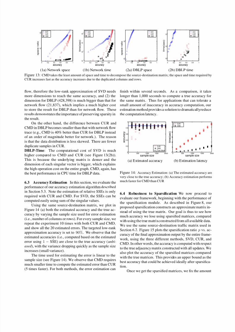
Figure 13: CMD takes the least amount of space and time to decompose the source-destination matrix; the space and time required by

CUR increases fast as the accuracy increases due to the duplicated columns and rows.

flow, therefore the low-rank approximation of SVD needs

more dimensions to reach the same accuracy, and (2) the

dimension for DBLP (428,398) is much bigger than that for

network flow (21,837), which implies a much higher cost

to store the result for DBLP than for network flow. These

results demonstrates the importance of preserving sparsity in

the result.

On the other hand, the difference between CUR and

CMD in DBLP becomes smaller than that with network flow

trace (e.g., CMD is 40% better than CUR for DBLP instead

of an order of magnitude better for network.). The reason

is that the data distribution is less skewed. There are fewer

duplicate samples in CUR.

DBLP-Time: The computational cost of SVD is much

higher compared to CMD and CUR (see Figure 13(2b)).

This is because the underlying matrix is denser and the

dimension of each singular vector is bigger, which explains

the high operation cost on the entire graph. CMD, again, has

the best performance in CPU time for DBLP data.

6.3 Accuracy Estimation In this section, we evaluate the

performance of our accuracy estimation algorithm described

in Section 5.3. Note the estimation of relative SSEs is only

required with CUR and CMD. For SVD, the SSEs can be

computed easily using sum of the singular values.

Using the same source-destination matrix, we plot in

Figure 14 (a) both the estimated accuracy and the true ac-

curacy by varying the sample size used for error estimation

(i.e., number of columns or rows). For every sample size, we

repeat the experiment 10 times with both CUR and CMD,

and show all the 20 estimated errors. The targeted low-rank

approximation accuracy is set to 90%. We observe that theestimated accuracies (i.e., computed based on the estimated

error using 1 − ˜SSE) are close to the true accuracy (unbi-

ased ), with the variance dropping quickly as the sample size

increases (small variance).

The time used for estimating the error is linear to the

sample size (see Figure 14). We observe that CMD requires

much smaller time to compute the estimated error than CUR

(5 times faster). For both methods, the error estimation can

finish within several seconds. As a comparison, it takes

longer than 1,000 seconds to compute a true accuracy for

the same matrix. Thus for applications that can tolerate a

small amount of inaccuracy in accuracy computation, our

estimation method provides a solution to dramaticallyreduce

the computation latency.

0 500 1000 1500 20000

0.2

0.4

0.6

0.8

1

a c c u r a c y

sample size

CURCMDTrue Value

0 500 1000 1500 20000

1

2

3

4

5

6

t i m e ( s e c )

sample size

CURCMD

(a) Estimated accuracy (b) Estimation latency

Figure 14:Accuracy Estimation: (a) The estimated accuracy are

very close to the true accuracy; (b) Accuracy estimation performs

much faster for CMD than CUR

6.4 Robustness to Sparsification We now proceed to

evaluate our framework, beginning with the performance of

the sparsification module. As described in Figure 8, our

proposed sparsification constructs an approximate matrix in-

stead of using the true matrix. Our goal is thus to see how

much accuracy we lose using sparsified matrices, compared

with using the true matrixconstructed from all available data.

We use the same source-destination traffic matrix used in

Section 6.2. Figure 15 plots the sparsification ratio p vs. ac-

curacy of the final approximation output by the entire frame-

work, using the three different methods, SVD, CUR, and

CMD. In other words, the accuracy is computed with respect

to the true adjacency matrix constructed with all updates. We

also plot the accuracy of the sparsified matrices compared

with the true matrices. This provides an upper bound as the

best accuracy that could be achieved ideally after sparsifica-

tion.

Once we get the sparsified matrices, we fix the amount



of space to use for the three different methods. We observe

that the accuracy of CMD is very close to the upper bound

ideal case. The accuracies achieved by all three methods do

not drop much as the sparsification ratio decreases, suggest-

ing the robustness of these methods to missing data. These

results indicate that we can dramatically reduce the number

of raw event records to sample without affecting the accuracymuch.

0 0.2 0.4 0.6 0.8 10

0.2

0.4

0.6

0.8

1

a c c u r a c y

sparsification ratio

SparsificationSVDCURCMD

Figure 15: Sparsification: it incurs small performance penalties,

for all algorithms.

In summary, CMD consistently out performs traditional

method SVD and the state of art method CUR on all experi-

ments. Next we will illustrate some applications of CMD in

practice.

7 Applications and Mining Case Study

In this section, we illustrate how CMD and our framework

can be applied in practice using two example applications:

(1) anomaly detection on a single matrix (i.e., a static

graph) and (2) storage, historical analysis, and real-time

monitoring of multiple matrices evolving over time (i.e.,dynamic graphs). For each application, we perform case

studies using real data sets.

7.1 Anomaly Detection Given a large static graph, how

do we efficiently determine if certain nodes are outliers, that

is, which rows or columns are significantly different than the

rest? And how do we identify them? In this section, we

consider anomaly detection on a static graph, with the goal

of finding abnormal rows or columns in the corresponding

adjacency matrix. CMD can be easily applied for mining

static graphs. We can detect static graph anomalies using

the SSE along each row or column as the potential indicators

after matrix decomposition.

A real world example is to detect abnormal hosts from

a static traffic matrix, which has often been an important but

challenging problem for system administrators. Detecting

abnormal behavior of host communication patterns can help

identify malicious network activities or mis-configuration

errors. In this case study, we focus on the static source-

destination matrices constructed from network traffic (every

column and row corresponds to a source and destination,

Ratio 20% 40% 60% 80% 100%

Source IP 0.9703 0.9830 0.9727 0.8923 0.8700

Destination IP 0.9326 0.8311 0.8040 0.7220 0.6891

Table 3: Network anomaly detection: precision is high for all spar-

sification ratios (the detection false positive rate = 1 − precision).

respectively), and use the SSEs on rows and columns to

detect the following two types of anomalies:

Abnormal source hosts: Hosts that send out abnormal traf-

fic, for example, port-scanners, or compromised “zombies”.

One example of abnormal source hosts are scanners that send

traffic to a large number of different hosts in the system.

Scanners are usually hosts that are already compromised by

malicious attacks such as worms. Their scanning activities

are often associated with further propagating the attack by

infecting other hosts. Hence it is important to identify and

quarantine these hosts accurately and quickly. We proposeto flag a source host as “abnormal”, if its row has a high re-

construction error.

Abnormal destination hosts: Examples include targets of

denial of service attacks (DoS), or targets of distributed

denialof service (DDoS). Hosts that receive abnormal traffic.

An example abnormal destination host is one that has been

under denial of service attacks by receiving a high volume

of traffic from a large number of source hosts. Similarly, our

criterion is the (column) reconstruction error.

Experimental setup: We randomly pick an adjacency ma-

trix from normal periods with no known attacks. Due to

the lack of detailed anomaly information, we manually in-

ject anomalies into the selected matrix using the followingmethod: (1) Abnormal source hosts: We randomly select a

source host and then set all the corresponding row entries to

1, simulating a scanner host that sends flows to every other

host in the network. (2) Abnormal destination hosts: Simi-

lar to scanner injection, we randomly pick a column and set

90% of the corresponding column entries to 1, assuming the

selected host is under denial of service attack from a large

number of hosts.

There are two additional input parameters: sparsifica-

tion ratio and the number of sampled columns and rows. We

vary the sparsification ratio from 20% to 100% and set the

sampled columns (and rows) to 500.

Performance metrics: We use detection precision as our

metric. We sort hosts based their row SSEs and column

SSEs, and extract the smallest number of top ranked hosts

(say k hosts) that we need to select as suspicious hosts, in

order to detect all injected abnormal host (i.e., recall = 100%with no false negatives). Precision thus equals 1/k, and the

false positive rate equals 1 − precision.

We inject only one abnormal host each time. And we

repeat each experiment 100 times and take the mean.



Results: Table 3(a) and (b) show the precision vs. sparsifica-

tion ratio for detecting abnormal source hosts and abnormal

destination hosts, respectively. Although the precision re-

mains high for both types of anomaly detection, we achieve

a higher precision in detecting abnormal source hosts than

detecting the abnormal destinations. One reason is that scan-

ners talk to almost all other hosts while not all hosts willlaunch DOS attacks to a targeted destination. In other words,

there are more abnormal entries for a scanner than for a host

under denial of service attack. Most of the false positives are

actually from servers and valid scanning hosts, which can be

easily removed based on the prior knowledge of the network

structure.

Our purpose of this case study is not to present the

best algorithm for anomaly detection, but to show the great

potential of using efficient matrix decomposition as a new

method for anomaly detection. Such approach may achieve

similar or better performance than traditional methods but

without expensive analysis overhead.

7.2 Time-Evolving Monitoring In this section, we con-

sider the application of monitoring dynamic graphs. Using

our proposed process, we can dynamically construct and an-

alyze time-evolving graphs from real-time application data.

One usage of the output results is to provide compact storage

for historical analysis. In particular, for every timestamp t,we can store only the sampled columns and rows as well as

the estimated approximation error ˜SSE t in the format of a

tuple (Ct,Rt, ˜SSE t).

Furthermore, the approximation error (SSE) is useful

for monitoring dynamic graphs, since it gives an indication

of how much the global behavior can be captured using thesamples. In particular, we can fix the sparsification ratio and

the CMD sample size, and then compare the approximation

error over time. A timestamp with a large error or a time

interval (multiple timestamps) with a large average error

implies structural changes in the corresponding graph, and

is worth additional investigation.

To make our discussion concrete, we illustrate the appli-

cation of time-evolving monitoring using both the network

traffic matrices and the DBLP matrices.

Network over time: For network traffic, normal host com-

munication patterns in a network should roughly be similar

to each other over time. A sudden change of approximation

accuracy (i.e., 1− ˜SSE ) suggests structural changes of com-munication patterns since the same approximation procedure

can no longer keep track of the overall patterns.

Figure 16(b) shows the approximation accuracy over

time, using 500 sampled rows and columns without dupli-

cates (out of 21K rows/columns). The overall accuracy re-

mains high. But an unusual accuracy drop occurs during the

period from hour 80 to 100. We manually investigate into the

trace further, and indeed find the onset of worm-like hierar-

chical scanning activities. For comparison, we also plot the

percentage of non-zero matrix entries generated each hour

over time in Figure 16(a), which is a standard method for

network anomaly detection based on traffic volume or dis-

tinct number of connections. Although such statistic is rel-

atively easier to collect, the total number of traffic entries

is not always an effective indicator of anomaly. Notice thatduring the same period of hour 80 to 100, the percentage of

non-zero entries is not particularly high. Only when the in-

fectious activity became more prevalent (after hour 100), we

can see an increase of the number of non-zero entries. Our

framework can thus potentially help detect abnormal events

at an earlier stage.

50 100 150

2

4

6

8x 10

−5

n o n z e r o p e r c e n t a g e

hours50 100 150

0

0.5

1

hours

A

c c u r a c y

(a) Nonzero entries over time (b) Accuracy over time

Figure 16: Network flow over time: we can detect anomalies

by monitoring the approximation accuracy (b), while traditional

method based on traffic volume cannot do (a).

DBLP over time: For the DBLP setting, we monitor the ac-

curacy over the 25 years by sampling 300 conferences (out of

3,659 conferences) and 10 K authors (out of 428K authors)

each year. Figure 17(b) shows that the accuracy is high ini-

tially, but slowly drops over time. The interpretation is that

the number of authors and conferences (nonzero percentage)

increases over time (see Figure 17(a)), suggesting that we

need to sample more columns and rows to achieve the same

high approximation accuracy.

1980 1985 1990 1995 2000 20050

1

2

3

4

5x 10

−5

n o n z e r o

p e r c e n t a g e

year1980 1985 1990 1995 2000 20050

0.2

0.4

0.6

0.8

1

Year

A c c u r a c y

(a) Nonzero entries over time (b) Accuracy over time

Figure 17: DBLP over time: The approximation accuracy drops

slowly as the graphs grow denser.

In summary, our exploration of both applications sug-

gest that CMD has great potential for discovering patterns

and anomalies for dynamic graphs too.



8 Conclusion

We studied the problem of efficiently discovering patterns

and anomalies from large graphs, like traffic matrices, both

in the static case, as well as when they evolve over time. The

contributions are the following:

• New matrix decomposition method: CMD generateslow-rank, sparse matrix approximations. We proved

that CMD gives exactly the same accuracy like CUR,

but in much less space (Theorem 4.1).

• High-rate time evolving graphs: Extension of CMD,

with careful sampling, and fast estimation of the recon-

struction error, to spot anomalies.

• Speed and space: Experiments on several real datasets,

one of which is >100Gb of real traffic data, show that

CMD achieves up to 10 times less space and less time

than the competition.

• Effectiveness: CMD found anomalies that were verified

by domain experts, like the anomaly in Figure 16

Future work could focus on the time window size:currently, the window size is 1 time-tick. Longer windowsmight be able to reveal long-term trends, like, e.g., low-rate port-scanners in network intrusion. The choice of theoptimal window size is a research challenge.

9 Acknowledgement

We are pleased to acknowledge Petros Drineas and Michael Ma-

honey for the insightful comments on the work. This material is

based upon work supported by the National Science Foundation

under Grants No. SENSOR-0329549 EF-0331657 IIS-0326322IIS-0534205 CNS-0433540 ANI-0331653. This work is also sup-

ported in part by the Pennsylvania Infrastructure Technology Al-

liance (PITA), with funding from Yahoo! research, Intel, NTT and

Hewlett-Packard and U.S. Army Research Office contract number

DAAD19-02-1-0389. Any opinions, findings, and conclusions or

recommendations expressed in this material are those of the au-

thor(s) and do not necessarily reflect the views of the National Sci-

ence Foundation, or other funding parties.

References

[1] http://www.informatik.uni-trier.de/ ley/db/.

[2] D. Achlioptas and F. McSherry. Fast computation of low rank

matrix approximations. In STOC , 2001.[3] B. Babcock, S. Babu, M. Datar, R. Motwani, and J. Widom.

Models and issues in data stream systems. In PODS, 2002.

[4] G. Cormode, M. Datar, P. Indyk, and S. Muthukrishnan.

Comparing data streams using hamming norms (how to zero

in). TKDE , 15(3), 2003.

[5] G. Cormode and S. Muthukrishnan. Space efficient mining of

multigraph streams. In PODS, 2005.

[6] S. C. Deerwester, S. T. Dumais, T. K. Landauer, G. W.

Furnas, and R. A. Harshman. Indexing by latent semantic

analysis. Journal of the American Society of Information

Science, 41(6):391–407, 1990.

[7] P. Domingos and M. Richardson. Mining the network value

of customers. KDD, pages 57–66, 2001.

[8] P. Drineas, R. Kannan, and M. Mahoney. Fast monte carlo al-

gorithms for matrices i: Approximating matrix multiplication.

SIAM Journal of Computing, 2005.[9] P. Drineas, R. Kannan, and M. Mahoney. Fast monte carlo al-

gorithms for matrices ii: Computing a low rank approximation

to a matrix. SIAM Journal of Computing, 2005.

[10] P. Drineas, R. Kannan, and M. Mahoney. Fast monte carlo

algorithms for matrices iii: Computing a compressed approx-

imate matrix decomposition. SIAM Journal of Computing,

2005.

[11] P. Drineas, I. Kerenidis, and P. Raghavan. Competitive

recommendation systems. In STOC , pages 82–90, 2002.

[12] M. Faloutsos, P. Faloutsos, and C. Faloutsos. On power-law

relationships of the internet topology. In SIGCOMM , pages

251–262, 1999.

[13] V. Ganti, J. Gehrke, and R. Ramakrishnan. Mining data

streams under block evolution. SIGKDD Explor. Newsl., 3(2),2002.

[14] P. B. Gibbons and Y. Matias. New sampling-based summary

statistics for improving approximate query answers. In SIG-

MOD, 1998.

[15] G. H. Golub and C. F. V. Loan. Matrix Computation. Johns

Hopkins, 3rd edition, 1996.

[16] S. Guha, D. Gunopulos, and N. Koudas. Correlating syn-

chronous and asynchronous data streams. In KDD, 2003.

[17] P. Indyk. Stable distributions, pseudorandom generators,

embeddings and data stream computation. In FOCS, 2000.

[18] I. Jolliffe. Principal Component Analysis. Springer, 2002.

[19] F. Korn, H. V. Jagadish, and C. Faloutsos. Efficiently sup-

porting ad hoc queries in large datasets of time sequences. In

SIGMOD, pages 289–300, 1997.[20] R. Kumar, P. Raghavan, S. Rajagopalan, and A. Tomkins.

Extracting large-scale knowledge bases from the web. In

VLDB, 1999.

[21] J. Leskovec, J. Kleinberg, and C. Faloutsos. Graphs over

time: Densification laws, shrinking diameters and possible

explanations. In SIGKDD, 2005.

[22] S. Muthukrishnan. Data streams: algorithms and applica-

tions, volume 1. Foundations and Trends. in Theoretical Com-

puter Science, 2005.

[23] C. H. Papadimitriou, H. Tamaki, P. Raghavan, and S. Vem-

pala. Latent semantic indexing: A probabilistic analysis.

pages 159–168, 1998.

[24] S. Papadimitriou, J. Sun, and C. Faloutsos. Streaming pattern

discovery in multiple time-series. In VLDB, 2005.[25] J. S. Vitter. Random sampling with a reservoir. ACM Trans.

Math. Software, 11(1):37–57, 1985.

[26] X. Yan, P. S. Yu, and J. Han. Substructure similarity search in

graph databases. In SIGMOD, 2005.

compact matrix decomposition

Documents