comparative advantage and optimal trade policy
TRANSCRIPT

Comparative Advantage and Optimal Trade Policy∗
Arnaud Costinot
MIT
Dave Donaldson
MIT
Jonathan Vogel
Columbia
Iván Werning
MIT
October 2013
Abstract
The theory of comparative advantage is at the core of neoclassical trade theory. Yet we
know little about its implications for how nations should conduct their trade policy.
For example, should import sectors with weaker comparative advantage be protected
more? Conversely, should export sectors with stronger comparative advantage be
subsidized less? In this paper we take a first stab at exploring these issues in the con-
text of a canonical Ricardian model. Our main results imply that optimal import tariffs
should be uniform, whereas optimal export subsidies should be weakly decreasing
with respect to comparative advantage, reflecting the fact that countries have more
room to manipulate prices in their comparative-advantage sectors.
∗We thank Gene Grossman as well as seminar participants at Brown and Princeton University for use-ful comments. Rodrigo Rodrigues Adao provided superb research assistance. Costinot and Donaldsonthank the National Science Foundation (under Grant SES-1227635) for research support. Vogel thanks thePrinceton International Economics Section for their support.

1 Introduction
Two of the most central questions in international economics are “Why do nations trade?”and “How should a nation conduct its trade policy?” The theory of comparative advan-tage is one of the most influential answers to the former question. Yet, it has had littleimpact on answers to the latter question. Our goal in this paper is to explore the relation-ship between comparative advantage and optimal trade policy.
Our main result can be stated as follows. Optimal trade taxes should be uniformacross imported goods and weakly monotone with respect to comparative advantageacross exported goods. Examples of optimal trade taxes include (i) a zero import tariffaccompanied by export taxes that are weakly increasing with comparative advantage or(ii) a uniform, positive import tariff accompanied by export subsidies that are weaklydecreasing with comparative advantage. While the latter pattern accords well with theobservation that countries tend to protect their least competitive sectors in practice, largersubsidies do not stem from a greater desire to expand production in less competitive sec-tors. Rather they reflect tighter constraints on the ability to exploit monopoly power bycontracting exports. Put simply, countries have more room to manipulate world prices intheir comparative-advantage sectors.
Our starting point is a canonical Ricardian model of trade. We focus on this modelbecause this is the oldest and simplest theory of comparative advantage as well the newworkhorse model for quantitative work in the field; see Eaton and Kortum (2012). Weconsider a world economy with two countries, Home and Foreign, one factor of produc-tion, labor, a continuum of goods, and Constant Elasticity of Substitution (CES) utility, asin Dornbusch et al. (1977), Wilson (1980), Eaton and Kortum (2002), and Alvarez and Lu-cas (2007). Labor productivity can vary arbitrarily across sectors in both countries. Homesets trade taxes in order to maximize domestic welfare, whereas Foreign is passive. In theinterest of clarity we assume no other trade costs in our baseline model.
In order to characterize the structure of optimal trade taxes, we use the primal ap-proach and consider first a fictitious planning problem in which the domestic governmentdirectly controls consumption and output decisions. Using Lagrange multiplier methods,we then show how to transform this infinite dimensional problem with constraints intoa series of simple unconstrained, low-dimensional problems. This allows us to derivesharp predictions about the structure of the optimal allocation. Finally, we demonstratehow that allocation can be implemented through trade taxes and relate optimal tradetaxes to comparative advantage.
Our approach is flexible enough to be used in more general environments that fea-
1

ture non-CES preferences and trade costs. In both extensions, we are able to show thatour main insights survive. In particular, the prediction that optimal trade taxes are uni-form across imported goods and weakly monotone with respect to comparative advan-tage holds without further qualification in a Ricardian model with uniform iceberg tradecosts.
Our approach can also be used for quantitative work. We apply our theoretical resultsto study the design of optimal trade policy in a world economy comprising two coun-tries: the United States and the Rest of the World. We consider two separate exercises.In the first one, all goods are assumed to be agricultural goods, whereas in the secondone, all goods are assumed to be manufactured goods. We find U.S. gains from tradeunder optimal trade taxes that are 20% larger than those obtained under laissez-faire forthe agricultural exercise and 33% larger for the manufacturing exercise. Interestingly, asignificant fraction of these gains arises from the use of trade taxes that are monotone incomparative advantage. Under an optimal uniform tariff, gains from trade for both theagriculture and manufacturing exercises would only be 9% larger than those obtainedunder laissez-faire. While these two-country examples are admittedly stylized, they sug-gest that the economic forces emphasized in this paper may be quantitatively importantas well. We hope that future quantitative work, in the spirit of Ossa (2011), will furtherexplore this issue in an environment featuring a large number of countries and a richgeography of trade costs.
Our paper makes two distinct contributions to the existing literature. The first oneis to study the relationship between comparative advantage and optimal trade taxes. Inhis survey of the literature, Dixit (1985) sets up the general problem of optimal taxes inan open economy as a fictitious planning problem and derives the associated first-orderconditions. As Bond (1990) demonstrates, such conditions impose very weak restrictionson the structure of optimal trade taxes. Hence, optimal tariff arguments are typically castusing simple general equilibrium models featuring only two goods or partial equilibriummodels. In such environments, characterizing optimal trade taxes reduces to solving theproblem of a single-good monopolist/monopsonist and leads to the prediction that theoptimal tariff should be equal to the inverse of the (own-price) elasticity of the foreignexport supply curve.1
In a canonical Ricardian model, countries buy and sell many goods whose prices de-pend on the entire vector of net imports through their effects on wages. Thus the (own-
1This idea has a long history in the international trade literature, going back to Torrens (1844) and Mill(1844). This rich history is echoed by recent theoretical and empirical work emphasizing the role of terms-of-trade manipulation in the analysis of optimal tariffs and its implication for the WTO; see Bagwell andStaiger (1990), Bagwell and Staiger (2011) and Broda et al. (2008).
2

price) elasticity of the foreign export supply curve no longer provides a sufficient statisticfor optimal trade taxes. Nevertheless our analysis shows that for any wage level, optimaltrade taxes must satisfy simple and intuitive properties. What matters for one of our mainresults is not the entire schedule of own-price and cross-price elasticities faced by a coun-try acting as a monopolist, which determines the optimal level of wages in a non-trivialmanner, but the cross-sectional variation in own-price elasticities across sectors holdingwages fixed, which is tightly connected to a country’s comparative advantage.
The paper most closely related to ours is Itoh and Kiyono (1987). They show that in aRicardian model with Cobb-Douglas preferences, export subsidies that are concentratedon “marginal” goods are always welfare-enhancing. Though the logic behind their resultis distinct from ours—a point we come back to in Section 4.3—it resonates well with ourfinding that, at the optimum, export subsidies should be weakly decreasing with com-parative advantage, so that “marginal” goods should indeed be subsidized more. Ouranalysis goes beyond the results of Itoh and Kiyono (1987) by considering a Ricardian en-vironment with general CES utility and, more importantly, by solving for optimal tradetaxes rather than providing examples of welfare-enhancing policies.2 Beyond general-ity, our results also shed light on the simple economics behind optimal trade taxes in acanonical Ricardian model: taxes should be monotone in comparative advantage becausecountries have more room to manipulate prices in their comparative-advantage sectors.
More broadly, these results have implications for the recent controversy regarding theconsequences, or lack thereof, of micro-level heterogeneity for the welfare gains fromtrade; see Helpman (2013) and Melitz and Redding (2013). In recent work, Arkolakis etal. (2012) have shown that, depending on how the question is framed, answers to micro-level questions may be of no consequence for predicting how international trade affectswelfare within a broad class of models. These results rely on calibrating certain macroresponses, holding them fixed across models. Helpman (2013) and Melitz and Redding(2013) offer a different perspective, where these behavioral responses are not held fixed.Regardless of this debatable choice, our paper emphasizes policy margins that bring outthe importance of micro structure. Our qualitative results—that trade taxes should bemonotone in comparative advantage—and our quantitative results—that such trade taxeslead to substantially larger welfare gains than uniform trade taxes—illustrate that thedesign of and the gains associated with optimal trade policy may crucially depend on theextent of micro-level heterogeneity. Here, micro-level data matter, both qualitatively andquantitatively, for answering the policy-relevant question: How should a nation conduct
2Opp (2009) also studies optimal trade taxes in a two-country Ricardian model with CES utility, but hisanalysis focuses on optimal tariffs that are uniform across goods.
3

its trade policy?3
The second contribution of our paper is technical. The problem of finding optimaltrade taxes in a canonical Ricardian model is infinite-dimensional (since there is a contin-uum of goods), non-concave (since indirect utility functions are quasi-convex in prices),and non-smooth (since the world production possibility frontier has kinks). To makeprogress on this question, we follow a three-step approach. First, we use the primal ap-proach to go from taxes to quantities. Second, we identify concave subproblems for whichgeneral Lagrangian necessity and sufficiency theorems problems apply. Third, we usethe additive separability of preferences to break down the maximization of a potentiallyinfinite-dimensional Lagrangian into multiple low-dimensional maximization problemsthat can be solved by simple calculus. Beyond the two extensions presented in this paper,the same approach could be used to study optimal trade taxes in economies with alterna-tive market structures, as in Bernard et al. (2003) and Melitz (2003), or multiple factors ofproduction, as in Dornbusch et al. (1980).
Our approach is related to recent work by Amador et al. (2006) and Amador and Bag-well (2013) who have used general Lagrange multiplier methods to study optimal dele-gation problems, including the design of optimal trade agreements, and to Costinot et al.(2013) who have used these methods together with the time-separable structure of pref-erences typically used in macro applications to study optimal capital controls. We brieflycome back to the specific differences between these various approaches in Section 3. Fornow, we note that like in Costinot et al. (2013), our approach heavily relies on the obser-vation, first made by Everett (1963), that Lagrange multiplier methods are particularlywell suited for studying “cell-problems,” i.e., additively separable maximization prob-lems with constraints. Given the importance of additively separable utility in the field ofinternational trade, we believe that these methods could prove useful beyond the ques-tion of how comparative advantage shapes optimal trade taxes. We hope that our paperwill help make such methods part of the standard toolbox of trade economists.
The rest of our paper is organized as follows. Section 2 describes our baseline Ricar-dian model. Section 3 sets up and solves the planning problem of a welfare-maximizingcountry manipulating its terms-of-trade. Section 4 shows how to decentralize the solutionof the planning problem through trade taxes and derive our main theoretical results. Sec-tion 5 establishes the robustness of our main insights to departures from CES utility andthe introduction of trade costs. Section 6 applies our theoretical results to the design of
3Though we have restricted ourselves to a Ricardian model for which the relevant micro-level dataare heterogeneous productivity levels across goods, not firms, the exact same considerations would makefirm-level data critical inputs for the design of optimal policy in imperfectly competitive models.
4

optimal trade taxes in the agricultural and manufacturing sectors. Section 7 offers someconcluding remarks. All formal proofs can be found in the Appendix.
2 Basic Environment
2.1 A Ricardian Economy
Consider a world economy with two countries, Home and Foreign, one factor of produc-tion, labor, and a continuum of goods indexed by i.4 Preferences at home are representedby the Constant Elasticity of Substitution (CES) utility,
U(c) ≡ ´i ui(ci)di,
where c ≡ (ci) ≥ 0 denotes domestic consumption; ui(ci) ≡ βi (c1−1/σ
i − 1)/(1− 1/σ)
denotes utility per good; σ ≥ 1 denotes the elasticity of substitution between goods; and(βi) are exogenous preference parameters such that
´i βidi = 1. Preferences abroad have
a similar form with asterisks denoting foreign variables. Production is subject to constantreturns to scale in all sectors. ai and a∗i denote the constant unit labor requirements athome and abroad, respectively. Labor is perfectly mobile across sectors and immobileacross countries. L and L∗ denote labor endowments at home and abroad, respectively.
2.2 Competitive Equilibrium
We are interested in situations in which the domestic government imposes ad-valoremtrade taxes cum subsidies, t ≡ (ti), whereas the foreign government does not imposeany tax. Each element ti ≥ 0 corresponds to an import tariff if good i is imported or anexport subsidy if it is exported. Conversely, each element ti ≤ 0 corresponds to an importsubsidy or an export tax. Tax revenues are rebated to domestic consumers through alump-sum transfer, T. Here, we characterize a competitive equilibrium for arbitrary taxes.Next, we will describe the domestic government’s problem that determines optimal taxes.
At home, domestic consumers choose consumption to maximize utility subject to theirbudget constraints; domestic firms choose output to maximize profits; the domestic gov-
4All subsequent results generalize trivially to economies with a countable number of goods. Wheneverthe integral sign “
´” appears, one should simply think of a Lebesgue integral. If the set of goods is finite or
countable, “´
” is equivalent to “∑.”
5

ernment balances its budget; and the labor market clears:
c ∈ argmaxc̃≥0{´
i ui(c̃i)di∣∣ ´
i pi (1 + ti) c̃idi ≤ wL + T}
, (1)
qi ∈ argmaxq̃i≥0 {pi (1 + ti) q̃i − waiq̃i} , (2)
T =´
i piti (ci − qi) di, (3)
L =´
i aiqidi, (4)
where p ≡ (pi) ≥ 0 is the schedule of world prices; w ≥ 0 is the domestic wage; andq ≡ (qi) ≥ 0 is domestic output. Similarly, utility maximization by foreign consumers,profit maximization by foreign firms, and labor market clearing abroad imply
c∗ ∈ argmaxc̃≥0{´
i u∗i (c̃i)di∣∣ ´
i pi c̃idi ≤ w∗L∗}
, (5)
q∗i ∈ argmaxq̃i≥0 {piq̃i − w∗a∗i q̃i} , (6)
L∗ =´
i a∗i q∗i di, (7)
where w∗ ≥ 0 is the foreign wage and q∗ ≡(q∗i)≥ 0 is foreign output. Finally, good
market clearing requiresci + c∗i = qi + q∗i . (8)
In the rest of this paper we define a competitive equilibrium with taxes as follows.
Definition 1. A competitive equilibrium with taxes corresponds to a schedule of trade taxest ≡ (ti), a lump-sum transfer, T, a pair of wages, w and w∗, a schedule of world prices, p ≡ (pi),a pair of consumption schedules, c ≡ (ci) and c∗ ≡
(c∗i), and a pair of output schedules, q ≡ (qi)
and q∗ ≡(q∗i), such that conditions (1)-(8) hold.
By Walras’ Law, competitive prices are only determined up to a normalization. Forexpositional purposes, we set prices throughout our analysis so that the marginal utilityof income in Foreign, that is the Lagrange multiplier associated with the budget constraintin (5), is equal to one. Hence the foreign wage, w∗, also represents the real income of theforeign consumer.
2.3 The Domestic Government’s Problem
We assume that Home is a strategic country that sets ad-valorem trade taxes t ≡ (ti) and alump-sum transfer T in order to maximize domestic welfare, whereas Foreign is passive.Formally, the domestic government’s problem is to choose the competitive equilibriumwith taxes, (t, T, w, w∗, p, c, c∗, q, q∗), that maximizes the utility of its representative con-
6

sumer, U (c). This leads to the following definition.
Definition 2. The domestic government’s problem is maxt,T,w≥0,w∗≥0,p≥0,c,c∗,q,q∗ U(c) subject toconditions (1)-(8).
The goal of the next two sections is to characterize how unilaterally optimal tradetaxes, i.e., taxes that prevail at a solution to the domestic government’s problem, varywith Home’s comparative advantage, as measured by the relative unit labor requirementsa∗i /ai. To do so we follow the public finance literature and use the primal approach as in,for instance, Dixit (1985).5 Namely, we will first approach the optimal policy problem ofthe domestic government in terms of a relaxed planning problem in which domestic con-sumption and domestic output can be chosen directly (Section 3). We will then establishthat the optimal allocation can be implemented through trade taxes and characterize thestructure of these taxes (Section 4).6
3 Optimal Allocation
3.1 Home’s Planning Problem
Throughout this section we focus on a fictitious environment in which there are no taxesand no competitive markets at home. Rather the domestic government directly controlsdomestic consumption, c, and domestic output, q, subject to the resource constraint,
´i aiqidi ≤ L. (9)
In other words, we ignore the equilibrium conditions associated with utility and profitmaximization by domestic consumers and firms; we ignore the government’s budget con-straint; and we relax the labor market clearing condition into inequality (9). We refer tothis relaxed maximization problem as Home’s planning problem.
Definition 3. Home’s planning problem is maxw∗≥0,p≥0,c≥0,c∗,q≥0,q∗ U(c) subject to conditions(5)-(9).
5An early application of the primal approach in international trade can be found in Baldwin (1948).6As will become clear, our main results do not hinge on this particular choice of instruments. We
choose to focus on trade taxes cum subsidies for expositional convenience because they are the simplesttax instruments required to implement the optimal allocation. It is well-known that one could allow forconsumption taxes, production taxes, or import tariffs that are not accompanied by export subsidies. Onewould then find that constraining consumption taxes to be equal to production taxes or import tariffs tobe equal to export subsidies, i.e. restricting attention to trade taxes cum subsidies, has no effect on theallocation that a welfare-maximizing government would choose to implement.
7

In order to prepare our discussion of optimal trade taxes, we will focus on the foreignwage, w∗, net imports m ≡ c− q, and domestic output, q, as the three key control vari-ables of the domestic government. To do so, we first establish that the conditions for anequilibrium in the rest of the world—namely, foreign utility maximization, foreign profitmaximization, and good and labor market clearing—can be expressed more compactly asa function of net imports and the foreign wage alone.
Lemma 1. (w∗, p, m, c∗, q∗) satisfies conditions (5)-(8) if and only if
pi = pi (mi, w∗) ≡ min{
u∗′i (−mi) , w∗a∗i}
, (10)
c∗i = c∗i (mi, w∗) ≡ max {−mi, d∗i (w∗a∗i )} , (11)
q∗i = q∗i (mi, w∗) ≡ max {0, mi + d∗i (w∗a∗i )} , (12)
for all i, with d∗i (·) ≡ u∗′−1i (·), u∗′i (−mi) ≡ ∞ if mi ≥ 0, and
´i a∗i q∗i (mi, w∗) di = L∗, (13)´i pi(mi, w∗)midi = 0. (14)
According to Lemma 1, when Home’s net imports are high, mi + d∗i (w∗a∗i ) > 0, foreign
firms produce good i, the world price is determined by their marginal costs, w∗a∗i , andforeign consumers demand d∗i (w
∗a∗i ).7 Conversely, when Home’s net imports are low,
mi + d∗i (w∗a∗i ) < 0, foreign firms do not produce good i, foreign consumption is equal to
Home’s net exports,−mi, and the world price is determined by the marginal utility of theforeign consumer, pi (mi, w∗) = u∗′i (−mi) . Equations (13) and (14), in turn, derive fromthe foreign labor market clearing condition and the foreign consumer’s budget constraint.
Let p (m, w∗) ≡ (pi(mi, w∗)), c∗ (m, w∗) ≡ (c∗i (mi, w∗)), and q∗ (m, w∗) ≡ (q∗i (mi, w∗))denote the schedule of equilibrium world prices, foreign consumption, and foreign out-put as a function of Home’s net imports and the foreign wage. Using Lemma 1, we cancharacterize the set of solutions to Home’s planning problem as follows.
Lemma 2. Suppose that (w0∗, p0, c0, c0∗, q0, q0∗) solves Home’s planning problem. Then(w0∗, m0 = c0 − q0, q0) solves
maxw∗≥0,m,q≥0
´i ui(qi + mi)di (P)
7Recall that good prices are normalized so that the marginal utility of income in Foreign is equal to one.
8
subject to
´i aiqidi ≤ L, (15)´
i a∗i q∗i (mi, w∗) di ≤ L∗, (16)´i pi(mi, w∗)midi ≤ 0. (17)
Conversely, suppose that(w0∗, m0, q0) solves (P). Then there exists a solution to Home’s plan-
ning problem,(w0∗, p0, c0, c0∗, q0, q0∗), such that p0 = p
(m0, w0∗), c0 = m0 + q0, c0∗ =
c∗(m0, w0∗), and q0∗ = q∗
(m0, w0∗).
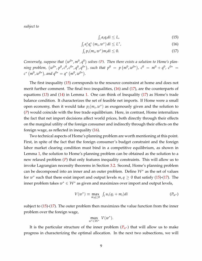
The first inequality (15) corresponds to the resource constraint at home and does notmerit further comment. The final two inequalities, (16) and (17), are the counterparts ofequations (13) and (14) in Lemma 1. One can think of Inequality (17) as Home’s tradebalance condition. It characterizes the set of feasible net imports. If Home were a smallopen economy, then it would take pi(mi, w∗) as exogenously given and the solution to(P) would coincide with the free trade equilibrium. Here, in contrast, Home internalizesthe fact that net import decisions affect world prices, both directly through their effectson the marginal utility of the foreign consumer and indirectly through their effects on theforeign wage, as reflected in inequality (16).
Two technical aspects of Home’s planning problem are worth mentioning at this point.First, in spite of the fact that the foreign consumer’s budget constraint and the foreignlabor market clearing condition must bind in a competitive equilibrium, as shown inLemma 1, the solution to Home’s planning problem can be obtained as the solution to anew relaxed problem (P) that only features inequality constraints. This will allow us toinvoke Lagrangian necessity theorems in Section 3.2. Second, Home’s planning problemcan be decomposed into an inner and an outer problem. Define W∗ as the set of valuesfor w∗ such that there exist import and output levels m, q ≥ 0 that satisfy (15)-(17). Theinner problem takes w∗ ∈ W∗ as given and maximizes over import and output levels,
V(w∗) ≡ maxm,q≥0
´i ui(qi + mi)di (Pw∗)
subject to (15)-(17). The outer problem then maximizes the value function from the innerproblem over the foreign wage,
maxw∗∈W∗
V(w∗).
It is the particular structure of the inner problem (Pw∗) that will allow us to makeprogress in characterizing the optimal allocation. In the next two subsections, we will
9

take the foreign wage w∗ as given and characterize the main qualitative properties ofthe solutions to (Pw∗). Since such properties will hold for all feasible values of the foreignwage, they will hold for the optimal one, w0∗ ∈ arg maxw∗∈W∗ V(w∗), and so by Lemma 2,they will apply to any solution to Home’s planning problem.8 Of course, for the purposesof obtaining quantitative results we also need to solve for the optimal foreign wage, w0∗,which we will do in Section 6.
Two observations will facilitate our analysis of the inner problem (Pw∗). First, as wewill formally demonstrate, (Pw∗) is concave, which implies that its solutions can be com-puted using Lagrange multiplier methods. Second, both the objective function and theconstraints in (Pw∗) are additively separable in (mi, qi). In the words of Everett (1963),(Pw∗) is a “cell-problem.” Using Lagrange multiplier methods, we will therefore be ableto transform an infinite dimensional problem with constraints into a series of simple un-constrained, low-dimensional problems.
3.2 Lagrangian Formulation
The Lagrangian associated with (Pw∗) is given by
L (m, q, λ, λ∗, µ; w∗) ≡´
i ui (qi + mi) di− λ´
i aiqidi− λ∗´
i a∗i q∗i (mi, w∗) di− µ´
i pi(mi, w∗)midi,
where λ ≥ 0, λ∗ ≥ 0, and µ ≥ 0 are the Lagrange multipliers associated with constraints(15)-(17). As alluded to above, a crucial property of L is that it is additively separable in(mi, qi). This implies that in order to maximize Lwith respect to (m, q), one simply needsto maximize the good-specific Lagrangian,
Li (mi, qi, λ, λ∗, µ; w∗) ≡ ui (qi + mi)− λaiqi − λ∗a∗i q∗i (mi, w∗)− µpi(mi, w∗)mi,
with respect to (mi, qi) for almost all i. In short, cell problems can be solved cell-by-cell,or in the present context, good-by-good.
Building on the previous observation, the concavity of (Pw∗), and Lagrangian necessityand sufficiency theorems—Theorem 1, p. 217 and Theorem 1, p. 220 in Luenberger (1969),respectively—we obtain the following characterization of the set of solutions to (Pw∗).
8This is a key technical difference between our approach and the approaches used in Amador et al.(2006), Amador and Bagwell (2013), and Costinot et al. (2013). The basic strategy here does not consistin showing that the maximization problem of interest can be studied using general Lagrange multipliermethods. Rather, the core of our approach lies in finding a subproblem to which these methods can beapplied. Section 5 illustrates the usefulness of this approach by showing how our results can easily beextended to environments with weakly separable preferences.
10

Lemma 3. For any w∗ ∈ W∗,(m0, q0) solves (Pw∗) if and only if
(m0
i , q0i)
solves
maxmi,qi≥0
Li (mi, qi, λ, λ∗, µ; w∗) (Pi)
for almost all i, with the Lagrange multipliers (λ, λ∗, µ) ≥ 0 such that constraints (15)-(17) holdwith complementary slackness.
Let us take stock. We started this section with Home’s planning problem, which isan infinite dimensional problem in consumption and output in both countries as wellas world prices and the foreign wage. By expressing world prices, foreign consumptionand foreign output as a function of net imports and the foreign wage (Lemma 1), wethen transformed it into a new planning problem (P) that only involves the scheduleof domestic net imports, m, domestic output, q, and the foreign wage, w∗, but remainsinfinitely dimensional (Lemma 2). Finally, in this subsection we have taken advantage ofthe concavity and the additive separability of the inner problem (Pw∗) in (mi, qi) to go fromone high-dimensional problem with constraints to many two-dimensional, unconstrainedmaximization problems (Pi) using Lagrange multiplier methods (Lemma 3).
The goal of the next subsection is to solve these two-dimensional problems in (mi, qi)
taking the foreign wage, w∗, and the Lagrange multipliers, (λ, λ∗, µ), as given. This is allwe will need to characterize qualitatively how comparative advantage affects the solu-tion of Home’s planning problem and, as discussed in Section 4, the structure of optimaltrade taxes. Once again, a full computation of optimal trade taxes will depend on theequilibrium values of (λ, λ∗, µ), found by using the constraints (15)-(17) and the value ofw∗ that maximizes V(w∗), calculations that we defer until Section 6.
3.3 Optimal Output and Net Imports
Our objective here is to find the solution(m0
i , q0i)
of
maxmi,qi≥0
Li (mi, qi, λ, λ∗, µ; w∗) ≡ ui (qi + mi)− λaiqi − λ∗a∗i q∗i (mi, w∗)− µpi(mi, w∗)mi.
While the economic intuition underlying our results will become transparent once we re-introduce trade taxes in Section 4, we focus for now on the simple maths through which(m0
i , q0i)
comes about. We proceed in two steps. First, we solve for the output level q0i (mi)
that maximizes Li (mi, qi, λ, λ∗, µ; w∗), taking mi as given. Second, we solve for the netimport level m0
i that maximizes Li(mi, q0
i (mi) , λ, λ∗, µ; w∗). The optimal output level is
then simply given by q0i = q0
i(m0
i).
11
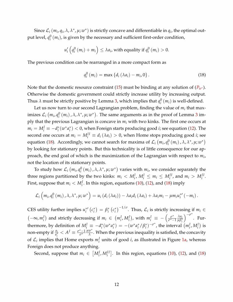
Since Li (mi, qi, λ, λ∗, µ; w∗) is strictly concave and differentiable in qi, the optimal out-put level, q0
i (mi), is given by the necessary and sufficient first-order condition,
u′i(
q0i (mi) + mi
)≤ λai, with equality if q0
i (mi) > 0.
The previous condition can be rearranged in a more compact form as
q0i (mi) = max {di (λai)−mi, 0} . (18)
Note that the domestic resource constraint (15) must be binding at any solution of (Pw∗).Otherwise the domestic government could strictly increase utility by increasing output.Thus λ must be strictly positive by Lemma 3, which implies that q0
i (mi) is well-defined.Let us now turn to our second Lagrangian problem, finding the value of mi that max-
imizes Li(mi, q0
i (mi) , λ, λ∗, µ; w∗). The same arguments as in the proof of Lemma 3 im-
ply that the previous Lagrangian is concave in mi with two kinks. The first one occurs atmi = MI
i ≡ −d∗i (w∗a∗i ) < 0, when Foreign starts producing good i; see equation (12). The
second one occurs at mi = MI Ii ≡ di (λai) > 0, when Home stops producing good i; see
equation (18). Accordingly, we cannot search for maxima of Li(mi, q0
i (mi) , λ, λ∗, µ; w∗)
by looking for stationary points. But this technicality is of little consequence for our ap-proach, the end goal of which is the maximization of the Lagrangian with respect to mi,not the location of its stationary points.
To study how Li(mi, q0
i (mi) , λ, λ∗, µ; w∗)
varies with mi, we consider separately thethree regions partitioned by the two kinks: mi < MI
i , MIi ≤ mi ≤ MI I
i , and mi > MI Ii .
First, suppose that mi < MIi . In this region, equations (10), (12), and (18) imply
Li
(mi, q0
i (mi) , λ, λ∗, µ; w∗)= ui (di (λai))− λaidi (λai) + λaimi − µmiu∗′i (−mi) .
CES utility further implies u∗′i(c∗i)= β∗i
(c∗i)−1/σ. Thus, Li is strictly increasing if mi ∈(
−∞, mIi)
and strictly decreasing if mi ∈(mI
i , MIi), with mI
i ≡ −(
σ∗σ∗−1
λaiµβ∗i
)−σ∗. Fur-
thermore, by definition of MIi ≡ −d∗i (w
∗a∗i ) = −(w∗a∗i /β∗i )−σ∗ , the interval
(mI
i , MIi)
isnon-empty if ai
a∗i< AI ≡ σ∗−1
σ∗µw∗
λ . When the previous inequality is satisfied, the concavity
of Li implies that Home exports mIi units of good i, as illustrated in Figure 1a, whereas
Foreign does not produce anything.Second, suppose that mi ∈
[MI
i , MI Ii]. In this region, equations (10), (12), and (18)
12

mi
Li
mIi MI
i 0 MI Ii
(a) ai/a∗i < AI .
mi
Li
MIi 0 MI I
i
(b) ai/a∗i ∈[AI , AI I).
mi
Li
MIi 0 MI I
i
(c) ai/a∗i = AI I .
mi
Li
MIi 0 MI I
i mI I Ii
(d) ai/a∗i > AI I .
Figure 1: Optimal net imports.
imply
Li
(mi, q0
i (mi) , λ, λ∗, µ; w∗)
= ui (di (λai))− λaidi (λai) + (λai − (λ∗ + µw∗) a∗i )mi − λ∗a∗i d∗i (w∗a∗i ) ,
which is strictly decreasing in mi if and only if aia∗i
< AI I ≡ λ∗+µw∗λ . When ai
a∗i∈[AI , AI I),
the concavity of Li implies that Home will export MIi units of good i, as illustrated in
Figure 1b. For these goods, Foreign is at a tipping point: it would start producing ifHome’s exports were to go down by any amount. In the knife-edge case, ai
a∗i= AI I , the
Lagrangian is flat between MIi and MI I
i so that any import level between MIi and MI I
i isoptimal, as illustrated in Figure 1c. In this situation, either Home or Foreign may produceand export good i.
Finally, suppose that MI Ii ≤ mi. In this region, equations (10), (12), and (18) imply
Li
(mi, q0
i (mi) , λ, λ∗, µ; w∗)= ui (mi)− (λ∗ + µw∗) a∗i mi − λ∗a∗i d∗i (w
∗a∗i ) ,
13

which is strictly increasing if mi ∈(
MI Ii , mI I
i)
and strictly decreasing if mi ∈(mI I
i , ∞),
with mI Ii ≡ di
((λ∗ + µw∗) a∗i
). Furthermore, by definition of MI I
i ≡ di (λai),(
MI Ii , mI I
i)
is non-empty if aia∗i
> AI I ≡ λ∗+µw∗λ . When this inequality is satisfied, the concavity of Li
implies that Home will import mI Ii units of good i, as illustrated in Figure 1d.
We summarize the above observations in the following proposition.
Proposition 1. If(m0
i , q0i)
solves (Pi), then optimal net imports are such that: (a) m0i = mI
i , ifai/a∗i < AI ; (b) m0
i = MIi , if ai/a∗i ∈
[AI , AI I); (c) m0
i ∈[MI
i , MI Ii]
if ai/a∗i = AI I ; and (d)m0
i = mI Ii , if ai/a∗i > AI I , where mI
i , MIi , mI I
i , MI I , AI , and AI I are the functions of w∗ and(λ, λ∗, µ) defined above.
Proposition 1 highlights the importance of comparative advantage, i.e., the cross-sectoral variation in the relative unit labor requirement ai/a∗i , for the structure of optimalimports. In particular, Proposition 1 implies that Home is a net exporter of good i onlyif ai/a∗i < AI I . Using Lemmas 2 and 3 to go from (Pi) to Home’s planning problem, thisleads to the following corollary.
Corollary 1. At any solution to Home’s planning problem, Home produces and exports goods inwhich it has a comparative advantage, ai/a∗i < AI I , whereas Foreign produces and exports goodsin which it has a comparative advantage, ai/a∗i > AI I .
According to Corollary 1, there will be no pattern of comparative advantage reversalsat an optimum. Like in a free trade equilibrium, there exists a cut-off such that Homeexports a good only if its relative unit labor requirement is below the cut-off. Of course,the value of that cut-off as well as the export levels will, in general, be different from thosein a free trade equilibrium.
4 Optimal Trade Taxes
We now demonstrate how to implement the solution of Home’s planning problem usingtrade taxes in a competitive equilibrium.
4.1 Wedges
Trade taxes cause domestic and world prices to differ from one another. To prepare ouranalysis of optimal trade taxes, we therefore start by describing the wedges, τ0
i , between
the marginal utility of the domestic consumer, u′i(c0i ) = βi
(c0
i)− 1
σ , and the world price,
14

p0i , that must prevail at any solution to Home’s planning problem:
τ0i ≡
u′i(c0
i)
p0i− 1. (19)
By Lemma 1, we know that if(w0∗, p0, c0, c0∗, q0, q0∗) solves Home’s planning problem—
and hence satisfies conditions (5)–(8)—then p0i = pi
(m0
i , w0∗). By Lemma 2, we also knowthat if
(w0∗, p0, c0, c0∗, q0, q0∗) solves Home’s planning problem, then
(w0∗, m0 = c0 − q0, q0)
solves (P). In turn, this implies that(m0 = c0 − q0, q0) solves (Pw∗) for w∗ = w0∗, and by
Lemma 3, that(m0
i , q0i)
solves (Pi) for almost all i. Accordingly, the good-specific wedgecan be expressed as
τ0i =
u′i(q0
i(m0
i)+ m0
i)
pi(m0
i , w0∗) − 1,
for almost all i, with pi(m0i , w0∗) and q0
i (m0i ) given by equations (10) and (18) and m0
isatisfying conditions (a)-(d) in Proposition 1. This further implies
τ0i =
σ∗−1
σ∗ µ0 − 1, if aia∗i
< AI ≡ σ∗−1σ∗
µ0w0∗
λ0 ;λ0ai
w0∗a∗i− 1, if AI < ai
a∗i≤ AI I ≡ µ0w0∗+λ0∗
λ0 ;λ0∗w0∗ + µ0 − 1, if ai
a∗i> AI I .
(20)
Since AI < AI I , we see that good-specific wedges are (weakly) increasing with ai/a∗i .For goods that are exported, ai/a∗i < AI I , the magnitude of the wedge depends on thestrength of Home’s comparative advantage. It attains its minimum value, σ∗−1
σ∗ µ0 − 1,for goods such that ai/a∗i < AI and increases linearly with ai/a∗i for goods such thatai/a∗i ∈ (AI , AI I). For goods that are imported, ai/a∗i > AI I , wedges are constant andequal to their maximum value, λ0∗
w0∗ + µ0 − 1.
4.2 Comparative Advantage and Trade Taxes
Let us now demonstrate that any solution(w0∗, p0, c0, c0∗, q0, q0∗) to Home’s planning
problem can be implemented by constructing a schedule of trade taxes, t0 = τ0, and alump-sum transfer, T0 =
´i piτ
0i m0
i di. Since the domestic government’s budget constraintis satisfied by construction and the resource constraint (9) must bind at any solution toHome’s planning problem, equations (3) and (4) trivially hold. Thus we only need tocheck that we can find a domestic wage, w0, such that the conditions for utility and profitmaximization by domestic consumers and firms at distorted local prices p0
i(1 + t0
i), i.e.,
conditions (1) and (2), are satisfied as well.
15

Consider first the problem of a domestic firm. At a solution to Home’s planning prob-lem, we have already argued in Section 3.3 that for almost all i,
u′i(
q0i + m0
i
)≤ λ0ai, with equality if q0
i > 0.
By definition of τ0, we also know that u′i(q0
i + m0i)= u′i
(c0
i)= p0
i(1 + τ0
i). Thus if
t0i = τ0
i , thenp0
i
(1 + t0
i
)≤ λ0ai, with equality if q0
i > 0. (21)
This implies that condition (2) is satisfied, with the domestic wage in the competitiveequilibrium given by the Lagrange multiplier on the labor resource constraint, w0 = λ0.
Let us turn to the domestic consumer’s problem. By definition of τ0, if t0i = τ0
i , then
u′i(
c0i
)= p0
i
(1 + t0
i
).
Thus for any pair of goods, i1 and i2, we have
u′i1
(c0
i1
)u′i2
(c0
i2
) =1 + t0
i11 + t0
i2
p0i1
p0i2
. (22)
Hence, the domestic consumer’s marginal rate of substitution is equal to the domesticrelative price. By Lemma 1, we know that trade must be balanced at a solution to Home’splanning problem,
´i p0
i m0i di = 0. Together with T0 =
´i piτ
0i m0
i di =´
i pit0i m0
i di, thisimplies ´
i p0i(1 + t0
i)
c0i di =
´i p0
i(1 + t0
i)
q0i di + T0. (23)
Since conditions (4) and (21) imply´
i p0i(1 + t0
i)
q0i di = λ0L, equation (23) implies that the
domestic consumer’s budget constraint must hold for w0 = λ0. Combining this observa-tion with equation (22), we can conclude that condition (1) must hold as well.
At this point, we have established that any solution(w0∗, p0, c0, c0∗, q0, q0∗) to Home’s
planning problem can be implemented by constructing a schedule of trade taxes, t0 =
τ0, and a lump-sum transfer, T0 =´
i piτ0i m0
i di. Since Home’s planning problem is arelaxed version of the domestic government’s problem, this immediately implies that(t0, T0, w0∗, p0, c0, c0∗, q0, q0∗) is a solution to the original problem. Conversely, suppose
that(t0, T0, w0∗, p0, c0, c0∗, q0, q0∗) is a solution to the domestic’s government problem,
then(w0∗, p0, c0, c0∗, q0, q0∗) must solve Home’s planning problem and, by condition (1),
16

aia∗i
t0i
AI AI I
t̄ = 0
AI
AI I − 1
(a) Export taxes.
aia∗i
t0i
AI AI I
0
t̄ = AI I
AI − 1
(b) Export subsidies and import tariffs.
Figure 2: Optimal trade taxes.
the optimal trade taxes t0 must satisfy
t0i =
u′i(c0
i)
νp0i− 1,
with ν > 0 the Lagrange multiplier on the domestic consumer’s budget constraint. Byequation (19), this implies that 1 + t0
i = 1ν (1 + τ0
i ). Combining this observation withequation (20), we obtain the following characterization of optimal trade taxes.
Proposition 2. At any solution of the domestic government’s problem, trade taxes, t0, are suchthat: (a) t0
i = (1 + t̄) (AI/AI I)− 1, if ai/a∗i < AI ; (b) t0i = (1 + t̄)
((ai/a∗i
)/AI I)− 1, if
ai/a∗i ∈[AI , AI I]; and (c) t0
i = t̄, if ai/a∗i > AI I , with t̄ > −1 and AI < AI I .
Proposition 2 states that optimal trade taxes vary with comparative advantage aswedges do. Trade taxes are at their lowest values, (1 + t̄) (AI/AI I)− 1, for goods in whichHome’s comparative advantage is the strongest, ai/a∗i < AI ; they are linearly increasingwith ai/a∗i for goods in which Home’s comparative advantage is in some intermediaterange, ai/a∗i ∈
[AI , AI I]; and they are at their highest value, t̄, for goods in which Home’s
comparative advantage is the weakest, ai/a∗i > AI I .Since only relative prices and hence relative taxes matter for domestic consumers and
firms, the overall level of taxes is indeterminate. This is an expression of Lerner symmetry,which is captured by the free parameter t̄ > −1 in the previous proposition. Figure 2illustrates two polar cases. In Figure 2a, there are no import tariffs, t̄ = 0, and all exportedgoods are subject to an export tax that rises in absolute value with comparative advantage.In Figure 2b, in contrast, all imported goods are subject to a tariff t̄ = AI I
AI − 1 ≥ 0, whereas
17

exported goods receive a subsidy that falls with comparative advantage. For expositionalpurposes, we focus in the rest of our discussion on the solution with zero import tariffs,t̄ = 0, as in Figure 2a.
To gain intuition about the economic forces that shape optimal trade taxes, considerfirst the case in which foreign preferences are Cobb-Douglas, σ∗ = 1, as in Dornbuschet al. (1977). In this case, AI = 0 so that the first region, ai/a∗i < AI , is empty. In thesecond region, ai/a∗i ∈
[AI , AI I], there is limit pricing: Home exports the goods and sets
export taxes t0i < t̄ = 0 such that foreign firms are exactly indifferent between producing
and not producing those goods, i.e., such that the world price satisfies p0i = λ0ai/ν(1 +
t0i ) = w0∗a∗i . The less productive are foreign firms relative to domestic firms, the more
room Home has to manipulate prices, and the bigger the export tax is (in absolute value).Finally, in the third region, ai/a∗i > AI I , relative prices are pinned down by the relativeunit labor requirements in Foreign. Since Home has no ability to manipulate these relativeprices, a uniform import tariff (here normalized to zero) is optimal.
In the more general case, σ∗ ≥ 1, as in Wilson (1980), Eaton and Kortum (2002), andAlvarez and Lucas (2007), the first region, ai/a∗i < AI , is no longer necessarily empty.The intuition, however, remains simple. In this region the domestic government has in-centives to charge a constant monopoly markup, proportional to σ∗/(σ∗ − 1). Specifically,the ratio between the world price and the domestic price is equal to 1/(1 + t0
i ) =σ∗
σ∗−1ν
µ0 .
In the region ai/a∗i ∈[AI , AI I], limit pricing is still optimal. But because AI is increasing
in σ∗, the extent of limit pricing, all else equal, decreases with the elasticity of demand inthe foreign market.
4.3 Discussion
Proposition 2 accords well with the observation that governments often protect a smallnumber of less competitive industries. Yet in our model, such targeted subsidies do notstem from a greater desire to expand production in these sectors. On the contrary, they re-flect tighter constraints on the ability to exploit monopoly power by contracting exports.According to Proposition 2, Home can only charge constant monopoly markups for ex-ported goods in which its comparative advantage is the strongest. For other exportedgoods, the threat of entry of foreign firms leads markups to decline together with Home’scomparative advantage.
An interesting issue is whether the structure of optimal trade taxes described in Propo-sition 2 crucially relies on the assumption that domestic firms are perfectly competitive.Since Home’s government behaves like a domestic monopolist competing à la Bertrand
18

against foreign firms, one may conjecture that if each good were produced by only onedomestic firm, then Home would no longer have to use trade taxes to manipulate prices:domestic firms would already manipulate prices under laissez-faire. This conjecture,however, is incorrect for two reasons.
The first reason is that although the government behaves like a monopolist, the do-mestic government’s problem involves non-trivial general equilibrium considerations.Namely, it internalizes the fact that by producing more goods at home, it lowers foreignlabor demand, which must cause a decrease in the foreign wage and an improvement ofHome’s terms-of-trade. These considerations are captured by the foreign resource con-straint (16) in Home’s planning problem. As we discuss in more details in Section 6.1,provided that the Lagrange multiplier associated with that constraint, λ0∗, is not zero, theoptimal level of the markup charged by the domestic government will be different fromwhat an individual firm would have charged, i.e., σ∗/ (σ∗ − 1).
The second reason is that to manipulate prices, Home’s government needs to affect thebehaviors of both firms and consumers: net imports depend both on supply and demand.If each good were produced by only one domestic firm, Home’s government would stillneed to impose good-varying consumption taxes that mimic the trade taxes describedabove (plus output subsidies that reflect general equilibrium considerations). Intuitively,if each good were produced by only one domestic firm, consumers would face monopolymarkups in each country, whereas optimality requires a wedge between consumer pricesat home and abroad.
As mentioned in the Introduction, our findings are related to the results of Itoh andKiyono (1987). They have shown that in the Ricardian model with Cobb-Douglas pref-erences considered by Dornbusch et al. (1977), export subsidies may be welfare enhanc-ing. A key feature of the welfare-enhancing subsidies that they consider is that they arenot uniform across goods; instead, they are concentrated on “marginal” goods. This isconsistent with our observation that, at the optimum, export taxes should be weakly de-creasing (in absolute value) with Home’s relative unit labor requirements, ai/a∗i , so that“marginal” goods should indeed be taxed less. The economic forces behind their results,however, are orthogonal to those emphasized in Proposition 2. Their results reflect thegeneral-equilibrium considerations alluded to above: by expanding the set of goods pro-duced at home, the domestic government can lower the foreign wage and improve itsterms-of-trade. In contrast, the heterogeneity of taxes across goods in Proposition 2 de-rives entirely from the structure of the inner problem (Pw∗), which takes the foreign wageas given. This implies, in particular, that Proposition 2 would still hold if Home were a“small” country in the sense that it could not affect the foreign wage.
19

5 Robustness
In this section we incorporate general preferences and trade costs into the Ricardianmodel presented in Section 2. Our goal is twofold. First, we want to demonstrate thatLagrange multiplier methods, and in particular our strategy of identifying concave cell-problems, remain well suited to analyzing optimal trade policy in these alternative envi-ronments. Second, we want to show that the central predictions derived in Section 4 donot crucially hinge on the assumption of CES utility or the absence of trade costs. To saveon space, we focus on sketching alternative environments and summarizing their mainimplications.
5.1 Preferences
While the assumption of CES utility is standard in the Ricardian literature—from Dorn-busch et al. (1977) to Eaton and Kortum (2002)—it implies strong restrictions on thedemand-side of the economy: own-price elasticities and elasticities of substitution areboth constant and pinned down by a single parameter, σ. In practice, price elasticitiesmay vary with quantities consumed and substitution patterns may vary across goods.For instance, one would expect two varieties of cars to be closer substitutes than, say, carsand bikes.
Here we relax the assumptions of Section 2 by assuming that: (i) Home’s preferencesare weakly separable over a discrete number of sectors, s ∈ S ≡ {1, ..., S}; and that:(ii) subutility within each sector, Us, is additively separable, though not necessarily CES.Specifically, we assume that Home’s preferences can be represented by the following util-ity function,
U = F(U1(c1), ...., US(cS)),
where F is a strictly increasing function; cs ≡ (ci)i∈I s is the consumption of goods insector s, with I s the set of goods that belongs to that sector; and Us is such that
Us (cs) =´
i∈I s usi (ci)di.
Foreign’s preferences are similar, and asterisks denote foreign variables. Section 2 cor-responds to the special case in which there is only one-sector, S = 1, and Us is CES,us
i (ci) ≡ βsi
(c
1−1/σs
i − 1)/
(1− 1/σs).9
9The analysis in this section trivially extends to the case in which only a subset of sectors have additivelyseparable utility. For this subset of sectors, and this subset only, our predictions would remain unchanged.
20

For expositional purposes, let us start by considering an intermediate scenario inwhich utility is not CES, but we maintain the assumption that there is only one sector,S = 1. It should be clear that the CES assumption is not crucial for the results derived inSections 2.2-3.2. In contrast, CES plays a key role in determining the optimal level of net
imports, mIi = −
(σ∗
σ∗−1λaiµβ∗i
)−σ∗, in Section 3.3 and, in turn, in establishing that trade taxes
are at their lowest values, (1 + t̄) (AI/AI I)− 1, for goods in which Home’s comparativeadvantage is the strongest in Section 4.2. Absent CES utility, trade taxes would still beuniform for goods in which Home’s comparative advantage is the weakest and linear inai/a∗i for goods in which Home’s comparative advantage is in some intermediate range.But for goods in which Home’s comparative advantage is the strongest, the optimal tradetax would now vary with the elasticity of demand, reflecting the incentives to chargedifferent monopoly markups.
Now let us turn to the general case with multiple sectors, S ≥ 1. With weaklyseparable preferences abroad, one can check that foreign consumption in each sector,cs∗ ≡
(c∗i)
i∈I s , must be such that
cs∗ ∈ argmaxc̃≥0{
Us∗ (c̃)|´
i∈I s psi c̃idi ≤ Es∗} ,
Accordingly, by the same argument as in Lemma 1, we can write the world price andforeign output for all s ∈ S and i ∈ I s as
psi (mi, w∗, Es∗) ≡ min
{us∗′
i (−mi) νs∗ (Es∗) , w∗a∗i}
, (24)
andqs∗
i (mi, w∗, Es∗) ≡ max {mi + ds∗i (w∗a∗i /νs∗ (Es∗)), 0} , (25)
where ν (Es∗) is the Lagrange multiplier associated with the constraint,´
i∈I s psi c̃idi ≤ Es∗.
In this situation, Home’s planning problem can still be decomposed into an outerproblem and multiple inner problems, one for each sector. At the outer level, the gov-ernment now chooses the foreign wage, w∗, together with the sectoral labor allocations inHome and Foreign, Ls and Ls∗, the sectoral trade deficits, Ds, subject to aggregate factormarket clearing and trade balance. At the inner level, the government treats Ls, Ls∗, Ds,and w∗ as constraints and maximizes subutility sector-by-sector. More precisely, Home’splanning problem can be expressed as
max{Ls,Ls∗,Ds}s∈S ,w∗∈W∗
F(V1(L1, L1∗, D1, w∗), ..., VS(LS, LS∗, DS, w∗))
21

subject to
∑s∈S Ls = L,
∑s∈S Ls∗ = L∗,
∑s∈S Ds = 0,
where the sector-specific value function is now given by
Vs (Ls, Ls∗, Ds, w∗) ≡ maxms,qs≥0
´i∈I s us
i (mi + qi)di
subject to
´i∈I s aiqidi ≤ Ls,´
i∈I s a∗i qs∗i (mi, w∗, w∗Ls∗ − Ds) di ≤ Ls∗,´
i∈I s psi (mi, w∗, w∗Ls∗ − Ds)midi ≤ Ds.
Given equations (24) and (25), the sector-specific maximization problem is of the sametype as in the baseline case (program P). As in Section 3.2, we can therefore reformu-late each infinite-dimensional sector-level problem into many two-dimensional, uncon-strained maximization problems using Lagrange multiplier methods. Within any sectorwith CES utility, all of our previous results hold exactly. Within any sector in which util-ity is not CES, our previous results continue to hold subject to the qualification aboutmonopoly markups discussed above.
5.2 Trade Costs
Trade taxes are not the only forces that may cause domestic and world prices to diverge.Here we extend our model to incorporate exogenous iceberg trade costs, δ ≥ 1, such thatif 1 unit of good i is shipped from one country to another, only a fraction 1/δ arrives. Inthe canonical two-country Ricardian model with Cobb-Douglas preferences consideredby Dornbusch et al. (1977), these costs do not affect the qualitative features of the equilib-rium beyond giving rise to a range of commodities that are not traded. We now show thatsimilar conclusions arise from the introduction of trade costs in our analysis of optimaltrade policy.
22

We continue to define world prices, pi, as those prevailing in Foreign and let
φ (mi) ≡{
δ, if mi ≥ 0,1/δ, if mi < 0,
(26)
denote the gap between domestic and world prices in the absence of trade taxes.As in our benchmark model, the domestic government’s problem can be reformulated
and transformed into many two-dimensional, unconstrained maximization problems us-ing Lagrange multiplier methods. In the presence of trade costs, Home’s objective is tofind the solution
(m0
i , q0i)
of the good-specific Lagrangian,
maxmi,qi≥0
Li (mi, qi, λ, λ∗, µ; w∗) ≡ ui (qi + mi)− λaiqi
− λ∗a∗i q∗i (mi, w∗)− µpi(mi, w∗)φ (mi)mi,
where pi (mi, w∗) and q∗i (mi, w∗) are now given by
pi (mi, w∗) ≡ min{
u∗′i (−miφ (mi)) , w∗a∗i}
, (27)
q∗i (mi, w∗) ≡ max{
miφ (mi) + d∗i (w∗a∗i ), 0
}. (28)
Compared to the analysis of Section 3, if Home exports −mi > 0 units abroad, thenForeign only consumes −mi/δ units. Conversely, if Home imports mi > 0 units fromabroad, then Foreign must export miδ units. This explains why φ (mi) appears in the twoprevious expressions.
The introduction of transportation costs leads to a new kink in the good-specific La-grangian. In addition to the kinks at mi = MI
i /δ ≡ −d∗i (w∗a∗i )/δ and mi = MI I
i ≡di (λai), there is now a kink at mi = 0, reflecting the fact that some goods may no longerbe traded at the solution of Home’s planning problem. As before, since we are notlooking for stationary points, this technicality does not complicate our problem. Whenmaximizing the good-specific Lagrangian, we simply consider four regions in mi space:mi < MI
i /δ, MIi /δ ≤ mi < 0, 0 ≤ mi < MI I
i , and mi ≥ MI Ii .
As in Section 3, if Home’s comparative advantage is sufficiently strong, ai/a∗i ≤ 1δ AI ≡
1δ
σ∗−1σ∗
µw∗λ , then optimal net imports are m0
i = δ1−σ∗mIi ≡ −
(σ∗
σ∗−1λaiµβ∗i
)−σ∗δ1−σ∗ . Similarly,
if Foreign’s comparative advantage is sufficiently strong, ai/a∗i > δAI I ≡ δλ∗+µw∗
λ , thenoptimal net imports are m0
i = δ−σ∗mI Ii ≡ di
((λ∗ + µw∗) δa∗i
). Relative to the benchmark
model, there is now a range of goods for which comparative advantage is intermediate,ai/a∗i ∈
(1δ AI I , δAI I
), in which no international trade takes place. For given values of
23

the foreign wage, w∗, and the Lagrange multipliers, λ, λ∗, µ, this region expands as tradecosts become larger, i.e., as δ increases.
Building on the previous observations, we obtain the following generalization of Propo-sition 1.
Proposition 3. Optimal net imports are such that: (a) m0i = δ1−σ∗mI
i , if ai/a∗i ≤ AI ; (b)m0
i = 1δ MI
i , if ai/a∗i ∈(
AI , 1δ AI I
); (c) m0
i ∈[
1δ MI
i , 0]
if ai/a∗i = 1δ AI I ; (d) m0
i = 0,
if ai/a∗i ∈(
1δ AI I , δAI I
); (e) m0
i ∈[0, MI I
i]
if ai/a∗i = δAI I ; and ( f ) m0i = δ−σ∗mI I
i , if
ai/a∗i > δAI I .
Using Proposition 3, it is straightforward to show, as in Section 4.1, that wedges acrosstraded goods are (weakly) increasing with Home’s comparative advantage. Similarly, asin Section 4.2, one can show that any solution to Home’s planning problem can be imple-mented using trade taxes and that the optimal taxes vary with comparative advantage aswedges do. In summary, our main theoretical results are also robust to the introductionof exogenous iceberg trade costs.
6 Applications
To conclude, we apply our theoretical results to two sectors: agriculture and manufactur-ing. Our goal is to take a first look at the quantitative importance of optimal trade taxesfor welfare, both in an absolute sense and relative to simpler uniform import tariffs.
In both applications, we compute optimal trade taxes as follows. First, we use Propo-sition 1 to solve for optimal imports and output given arbitrary values of the Lagrangemultipliers, (λ, λ∗, µ), and the foreign wage, w∗. Second, we use constraints (15)-(17) tosolve for the Lagrange multipliers. Finally, we find the value of the foreign wage thatmaximizes the value function V(w∗) associated with the inner problem. Given the opti-mal foreign wage, w0∗, and the associated Lagrange multipliers,
(λ0, λ0∗, µ0), we finally
compute optimal trade taxes using Proposition 2.
6.1 Agriculture
In many ways, agriculture provides the perfect environment in which to explore the quan-titative importance of our results. From a theoretical perspective, market structure is asclose as possible to the neoclassical ideal. From a measurement perspective, the scien-tific knowledge of agronomists provides a unique window into the structure of compar-ative advantage, as discussed in Costinot and Donaldson (2011). Finally, from a policy
24

perspective, agricultural trade taxes are pervasive and one of the most salient and con-tentious global economic issues, as illustrated by the World Trade Organization’s current,long-stalled Doha round.
Calibration. We start from the Ricardian economy presented in Section 2.1 and assumethat each good corresponds to one of 39 crops for which we have detailed productivitydata, as we discuss below. All crops enter utility symmetrically in all countries, βi =
β∗i = 1, with the same elasticity of substitution, σ = σ∗. Home is the United States andForeign is an aggregate of the rest of the world (henceforth R.O.W.). The single factor ofproduction is equipped land. We also explore how our results change in the presence ofexogenous iceberg trade costs, as in Section 5.2.
The parameters necessary to apply our theoretical results are: (i) the unit factor re-quirement for each crop in each country, ai and a∗i ; (ii) the elasticity of substitution, σ;(iii) the relative size of the two countries, L∗/L; and (iv) trade costs, δ, when relevant. Forsetting each crop’s unit factor requirements, we use data from the Global Agro-EcologicalZones (GAEZ) project from the Food and Agriculture Organization (FAO); see Costinotand Donaldson (2011). Feeding data on local conditions—e.g., soil, topography, eleva-tion and climatic conditions—into an agronomic model, scientists from the GAEZ projecthave computed the yield that parcels of land around the world could obtain if they wereto grow each of the 39 crops we consider in 2009.10 We set ai and a∗i equal to the aver-age hectare per ton of output across all parcels of land in the United States and R.O.W.,respectively.
The other parameters are chosen as follows. We set σ = 2.9 in line with the median es-timate of the elasticity of substitution across our 39 crops in Broda and Weinstein (2006).11
We set L = 1 and L∗ = 13 to match the relative acreage devoted to the 39 crops consid-ered, as reported in the FAOSTAT data in 2009. Finally, in the extension with trade costs,we set δ = 1.72 so that Home’s import share in the equilibrium without trade policymatches the U.S. agriculture import share—that is, the total value of U.S. imports overthe 39 crops considered divided by the total value of U.S. expenditure over those samecrops—in the FAOSTAT data in 2009, 11.1%.
Results. The left and right panels of Figure 3 report optimal trade taxes on all traded
10The GAEZ project constructs output per hectare predictions under different assumptions on a farmer’suse of complementary inputs (e.g. irrigation, fertilizers, and machinery). We use the measure that is con-structed under the assumption that irrigation and a “moderate” level of other inputs (fertilizers, machinery,etc.) are available to farmers.
11The elasticity of substitution estimated by Broda and Weinstein (2006) are available for 5-digit SITCsectors. When computing the median across our 39 crops, we restrict ourselves to 5-digit SITC codes thatcan be matched to raw versions of the 39 FAO crops.
25

0 0.4 0.8 1.2 1.6 2-60%
-40%
-20%
0
ai/a∗i
t0 i
0 0.4 0.8 1.2 1.6 2-60%
-40%
-20%
0
ai/a∗i
t0 i
Figure 3: Optimal trade taxes for the agricultural case. The left panel assumes no tradecosts, δ = 0. The right panel assumes trade costs, δ = 1.72.
crops i as a function of comparative advantage, ai/a∗i , in the calibrated examples withouttrade costs, δ = 1, and with trade costs, δ = 1.72, respectively.12 The region betweenthe two vertical lines in the right panel corresponds to goods that are not traded at thesolution of Home’s planning problem.
As discussed in Section 4.2, the overall level of taxes is indeterminate. Figure 3 fo-cuses on a normalization with zero import tariffs. In both cases, the maximum export taxis close to the optimal monopoly markup that a domestic firm would have charged on theforeign market, σ/ (σ− 1)− 1 ' 52.6%. The only difference between the two markupscomes from the fact that the domestic government internalizes the effect that the net im-ports of each good have on the foreign wage. Specifically, if the Lagrange multiplier onthe foreign resource constraint, λ0∗, was equal to zero, then the maximum export tax,which is equal AI/AI I − 1, would simplify into the firm-level markup, σ/ (σ− 1)− 1. Inother words, such general equilibrium considerations appear to have small effects on thedesign of optimal trade taxes for goods in which the U.S. comparative advantage is thestrongest. In light of the discussion in Section 4.3, these quantitative results suggest thatif domestic firms were to act as monopolists rather than take prices as given, then the do-mestic government could get close to the optimal allocation by only using consumption
12We compute optimal trade taxes, throughout this and the next subsection, by performing a grid searchover the foreign wage w∗ so as to maximize V(w∗). Since Foreign cannot be worse off under trade thanunder autarky—whatever world prices may be, there are gains from trade—and cannot be better off thanunder free trade—since free trade is a Pareto optimum, Home would have to be worse off—we restrictour grid search to values of the foreign wage between those that would prevail in the autarky and freetrade equilibria. Recall that we have normalized prices so that the Lagrange multiplier associated with theforeign budget constraint is equal to one. Thus w∗ is the real wage abroad.
26

No Trade Costs (δ = 1) Trade Costs (δ = 1.72)U.S. R.O.W. U.S. R.O.W.
Laissez-Faire 39.15% 3.02% 5.02% 0.25%Uniform Tariff 42.60% 1.41% 5.44% 0.16%Optimal Taxes 46.92% 0.12% 5.71% 0.04%
Table 1: Gains from trade for the agricultural case.
taxes that mimic the optimal trade taxes.The first and second columns of Table 1 display U.S. and R.O.W. welfare gains from
trade, i.e. the percentage change in total income divided by the CES price index rela-tive to autarky, in the baseline model with no trade costs, δ = 1. Three rows reportthe values of these gains from trade under each of three scenarios: (i) a laissez-faireregime with no U.S. trade taxes, (ii) a U.S. optimal uniform tariff, and (iii) U.S. opti-mal trade taxes as characterized in Proposition 2.13 In this example, optimal trade taxesthat are monotone in comparative advantage increase U.S. gains from trade in agricul-ture by 20% (46.92/39.15 − 1 ' 0.20) and decrease R.O.W.’s gains from trade by 96%(1− 0.12/3.02 ' 0.96). This suggests large inefficiencies from terms-of-trade manipula-tion at the world level. Interestingly, we also see that more than half of the previous U.S.gains arise from the use of non-uniform trade taxes (42.60/39.15− 1 ' 0.09).
The third and fourth columns of Table 1 revisit the previous three scenarios using themodel with trade costs, setting δ = 1.72. Not surprisingly, as the U.S. import shares goesdown from around 80% in the model without trade costs to its calibrated value of 11.1% inthe model with trade costs, gains from trade also go down by an order of magnitude, from39.15% to 5.02%. Yet, the relative importance of trade taxes that vary with comparativeadvantage remains fairly stable. Even with trade costs, gains from trade for the UnitedStates are 14% larger under optimal trade taxes than in the absence of any trade taxes(5.71/5.02− 1 ' 0.14) and about half of these gains arise from the use of non-uniformtrade taxes (5.44/5.02− 1 ' 0.08).
6.2 Manufacturing
There are good reasons to suspect that the quantitative results from Section 6.1 may notgeneralize to other tradable sectors. In practice, most traded goods are manufacturedgoods and the pattern of comparative advantage within those goods may be very differ-
13Scenarios (i) and (ii) are computed using the equilibrium conditions (1)-(8) in Section 2.2. In scenario(i), we set ti = 0 for all goods i. In scenario (ii) we set ti = t for all imported goods, we set ti = 0 for othergoods, and we do a grid search over t to find the optimal tariff.
27

ent than within agricultural products. We now explore the quantitative importance ofsuch considerations.
Calibration. As in the previous subsection, we focus on the baseline Ricardian economypresented in Section 2.1 and the extension to iceberg trade costs presented in Section 5.2.Home and Foreign still correspond to the United States and R.O.W., respectively, butwe now assume that each good corresponds to one of 400 manufactured goods that areproduced using equipped labor.14
Compared to agriculture, the main calibration issue is how to set unit factor require-ments. Since one cannot measure unit factor unit requirements directly for all manufac-tured goods in all countries, we follow the approach pioneered by Eaton and Kortum(2002) and assume that unit factor requirements are independently drawn across coun-tries and goods from an extreme value distribution whose parameters can be calibrated tomatch a few key moments in the macro data. In a two-country setting, Dekle et al. (2007)have shown that this approach is equivalent to assuming
ai =
(iT
) 1θ
and a∗i =
(1− iT∗
) 1θ
, (29)
with θ the shape parameter of the extreme value distribution, that is assumed to be com-mon across countries, and T and T∗ the scale parameters, that are allowed to vary acrosscountries. The good index i is equally spaced between 1/10, 000 and 1− 1/10, 000 for the400 goods in the economy.
Given the previous functional form assumptions, we choose parameters as follows.We set σ = 2.5 to match the median estimate of the elasticity of substitution across 5-digitSITC manufacturing sectors in Broda and Weinstein (2006), which is very close the valueused in the agricultural exercise.15 We set L = 1 and L∗ = 19.5 to match population in theU.S. relative to R.O.W., as reported by the World Bank in 2009. Since the shape parameterθ determines the elasticity of trade flows with respect trade costs, we set θ = 5, which isa typical estimate in the literature; see e.g. Anderson and Van Wincoop (2004) and Headand Mayer (2013). Given the previous parameters, we then set T = 5, 194.6 and T∗ = 1 sothat in the equilibrium without trade policy Home’s share of world GDP matches the U.S.share, 26%, as reported by the World Bank in 2009. Finally, in the extension with tradecosts, we now set δ = 1.44 so that Home’s import share in the equilibrium without trade
14The number of goods is chosen to balance computational burden against distance between our modeland models with a continuum of goods such as Eaton and Kortum (2002). We find similar results with othernumbers of goods.
15SITC manufacturing sectors include “Manufactured goods classified chiefly by material,” “Machineryand transport equipment,” and “Miscellaneous manufactured articles.”
28

0 0.2 0.4 0.6
-60%
-40%
-20%
0
ai/a∗i
t0 i
0 0.2 0.4 0.6
-60%
-40%
-20%
0
ai/a∗i
t0 i
Figure 4: Optimal trade taxes for the manufacturing case. The left panel assumes no tradecosts, δ = 0. The right panel assumes trade costs, δ = 1.44.
policy matches the U.S. manufacturing import share—i.e., total value of U.S. manufactur-ing imports divided by total value of U.S. expenditure in manufacturing—as reported inthe OECD STructural ANalysis (STAN) database in 2009, 24.7%.
Results. Figure 4 reports optimal trade taxes as a function of comparative advantage formanufacturing. As before, the left and right panels correspond to the models withoutand with trade costs, respectively, under a normalization with zero import tariffs. Likein the agricultural exercise of Section 6.1, we see that the maximum export tax is close tothe optimal monopoly markup that a domestic firm would have charged on the foreignmarket, σ/ (σ− 1)− 1 ' 66.7%, suggesting that the U.S. remains limited in its ability tomanipulate the foreign wage.
Table 2 displays welfare gains in the manufacturing sector. In the absence of tradecosts, as shown in the first two columns, gains from trade for the U.S. are 33% larger un-der optimal trade taxes than in the absence of any trade taxes (36.85/27.70− 1 ' 0.33) and86% smaller for the R.O.W. (1− 0.93/6.59 ' 0.86). This again suggests large inefficienciesfrom terms-of-trade manipulation at the world level. Compared to our agricultural ex-ercise, the share of the U.S. gains arising from the use of non-uniform trade taxes is noweven larger: more than two thirds (30.09/27.70− 1 ' 0.09).
As in Section 6.1, although the gains from trade are dramatically reduced by tradecosts—they go down to 6.18% and 2.02% for the U.S. and the R.O.W, respectively—theimportance of non-uniform trade taxes relative to uniform tariffs remains broadly sta-ble. In the presence of trade costs, gains from trade for the U.S., reported in the thirdcolumn, are 49% larger under optimal trade taxes than in the absence of any trade taxes
29

No Trade Costs (δ = 1) Trade Costs (δ = 1.44)U.S. R.O.W. U.S. R.O.W.
Laissez-Faire 27.70% 6.59% 6.18% 2.02%Uniform Tariff 30.09% 4.87% 7.31% 1.31%Optimal Taxes 36.85% 0.93% 9.21% 0.36%
Table 2: Gains from trade for the manufacturing case
(9.21/6.18− 1 ' 0.49), and more than half of these gains (7.31/6.18− 1 ' 0.18) arise fromthe use of trade taxes that vary with comparative advantage.
In contrast to the equivalence results of Arkolakis et al. (2012), the present resultsspeak well to the importance of micro-level heterogeneity for the design of and gains fromtrade policy. In this example, the functional form assumption imposed on the distribu-tion of unit labor requirements—equation (29)—implies that the model satisfies a gravityequation, as in Eaton and Kortum (2002). Conditional on matching the same trade elas-ticity and observed trade flows, the welfare changes associated with any uniform tradetax would be the same as in a simple Armington or Krugman (1980) model.16 This equiv-alence is reflected in the fact that the optimal uniform tariff in the present example isequal to the inverse of the trade elasticity multiplied by the share of foreign expendi-ture on foreign goods, as established by Gros (1987) in the context of the Krugman (1980)model. Since the United States is small compared to the rest of the world, this is roughly1/θ ' 20%, both in the exercises with and without trade costs. In contrast, Figure 4 showsthat the optimal export tax is around 60% and slowly decreasing in absolute value withForeign’s relative unit labor requirements. As shown in Table 2, these differences in de-sign are associated with significant welfare effects, at least within the scope of this simplecalibrated example.
Intuitively, the equivalence emphasized by Arkolakis et al. (2012) builds on the ob-servation that at the aggregate level, standard gravity models are equivalent to endow-ment models in which countries exchange labor and relative labor demand curves areiso-elastic. Hence, conditional on the shape of these demand curves, the aggregate im-plications of uniform changes in trade costs, i.e. exogenous demand shifters, must bethe same in all gravity models. For those particular changes, the micro-level assump-tions through which iso-elastic demand curves come about—either CES utility functionsin the Armington model or an extreme value distribution in the Eaton and Kortum (2002)
16The basic argument is the same as the one used by Arkolakis et al. (2012) to establish that the welfarechanges associated with any movement in iceberg trade costs are the same in the Armington, Krugman(1980), and Eaton and Kortum (2002) models. See Costinot and Rodríguez-Clare (2013) for a general dis-cussion of the effects of trade policy in gravity models.
30

model—are irrelevant. Trade taxes, however, are imposed on goods, not labor. Whenheterogeneous across goods, such taxes no longer act as labor demand shifters and theequivalence in Arkolakis et al. (2012) breaks down. This is precisely what happens whentrade taxes are chosen optimally.
7 Concluding Remarks
Comparative advantage is at the core of neoclassical trade theory. In this paper we havetaken a first stab at exploring how comparative advantage across nations affects the de-sign of optimal trade policy. In the context of a canonical Ricardian model of interna-tional trade we have shown that optimal trade taxes should be uniform across importedgoods and weakly monotone with respect to comparative advantage across exportedgoods. Specifically, export goods featuring weaker comparative advantage should betaxed less (or subsidized more) relative to those featuring stronger comparative advan-tage, reflecting the fact that countries have more room to manipulate world prices in theircomparative-advantage sectors.
Characterizing optimal trade taxes in a Ricardian model is technically non-trivial. Asmentioned in the Introduction, the maximization problem of the country manipulatingits terms-of-trade is infinite-dimensional, non-concave, and non-smooth. A second con-tribution of our paper is to show how to use Lagrange multiplier methods to solve suchproblems. Our basic strategy can be sketched as follows: (i) use the primal approach to gofrom taxes to quantities; (ii) identify concave subproblems for which general Lagrangiannecessity and sufficiency theorems apply; and (iii) use the additive separability of pref-erences to break the Lagrangian into multiple low-dimensional maximization problemsthat can be solved by simple calculus. Although we have focused on optimal trade taxesin a Ricardian model, our approach is well suited to other additively separable problems.For instance, one could use these tools to compute fully optimal policy in the Melitz (2003)model, extending the results of Demidova and Rodríguez-Clare (2009) and Felbermayr etal. (2011).
Finally, we have studied the quantitative implications of our theoretical results for thedesign of unilaterally optimal trade taxes in agricultural and manufacturing sectors. Inour applications, we have found that trade taxes that vary with comparative advantageacross goods lead to substantially larger welfare gains than optimal uniform trade taxes.In spite of the similarities between welfare gains from trade across models featuring dif-ferent margins of adjustment—see e.g. Atkeson and Burstein (2010) and Arkolakis et al.(2012)—this result illustrates that the design of and the gains associated with optimal
31

trade policy may crucially depend on the extent of heterogeneity at the micro level.
32

References
Alvarez, Fernando and Robert E. Lucas, “General Equilibrium Analysis of the Eaton-Kortum Model of International Trade,” Journal of Monetary Economics, 2007, 54 (6), 1726–1768.
Amador, Manuel and Kyle Bagwell, “The Theory of Optimal Delegation with an Appli-cation to Tariff Caps,” Econometrica, 2013, 81 (4), 1541–600.
, Ivan Werning, and George-Marios Angeletos, “Commitment versus Flexibility,”Econometrica, 2006, 74 (2), 365–396.
Anderson, James E. and Eric Van Wincoop, “Trade Costs,” Journal of Economic Literature,2004, 42 (3), 691–751.
Arkolakis, Costas, Arnaud Costinot, and Andres Rodríguez-Clare, “New Trade Models,Same Old Gains?,” American Economic Review, 2012, 102 (1), 94–130.
Atkeson, Andrew and Ariel Burstein, “Innovation, Firm Dynamics, and InternationalTrade,” Journal of Political Economy, 2010, 118 (3), 433–489.
Bagwell, Kyle and Robert W Staiger, “A Theory of Managed Trade,” American EconomicReview, September 1990, 80 (4), 779–95.
and Robert W. Staiger, “What Do Trade Negotiators Negotiate About? EmpiricalEvidence from the World Trade Organization,” American Economic Review, 2011, 101(4), 1238–73.
Baldwin, Robert E., “Equilibrium in International Trade: A Diagrammatic Approach,”Quarterly Journal of Economics, 1948, 62 (5), 748–762.
Bernard, Andew B., Jonathan Eaton, J. Bradford Jensen, and Samuel Kortum, “Plantsand Productivity in International Trade,” American Economic Review, 2003, 93 (4), 1268–1290.
Bond, Eric W, “The Optimal Tariff Structure in Higher Dimensions,” International Eco-nomic Review, February 1990, 31 (1), 103–16.
Broda, Christian, Nuno Limao, and David E. Weinstein, “Optimal Tariffs and MarketPower: The Evidence,” American Economic Review, December 2008, 98 (5), 2032–65.
33

Broda, Cristian and David Weinstein, “Globalization and the Gains from Variety,” Quar-terly Journal of Economics, 2006, 121 (2), 541–585.
Costinot, Arnaud and Andres Rodríguez-Clare, Trade Theory with Numbers: Quantifyingthe Consequences of Globalization, Vol. 4 of Handbook of International Economics, Elsevier,2013.
and Dave Donaldson, “How Large Are the Gains from Economic Integration? Theoryand Evidence from U.S. Agriculture, 1880-2002,” mimeo MIT, 2011.
, Guido Lorenzoni, and Ivan Werning, “A Theory of Capital Controls as DynamicTerms-of-Trade Manipulation,” mimeo MIT, 2013.
Dekle, Robert, Jonathan Eaton, and Samuel Kortum, “Unbalanced Trade,” NBER work-ing paper 13035, 2007.
Demidova, Svetlana and Andres Rodríguez-Clare, “Trade policy under firm-level het-erogeneity in a small economy,” Journal of International Economics, 2009, 78 (1), 100–112.
Dixit, Avinash, “Tax policy in open economies,” in A. J. Auerbach and M. Feldstein,eds., Handbook of Public Economics, Vol. 1 of Handbook of Public Economics, Elsevier, 1985,chapter 6, pp. 313–374.
Dornbusch, Rudiger S., Stanley Fischer, and Paul A. Samuelson, “Comparative Ad-vantage, Trade, and Payments in a Ricardian Model with a Continuum of Goods,” TheAmerican Economic Review, 1977, 67 (5), 823–839.
Dornbusch, Rudiger, Stanley Fischer, and Paul Samuelson, “Heckscher-Ohlin TradeTheory with a Continuum of Goods,” Quarterly Journal of Economics, 1980, 95 (2), 203–224.
Eaton, Jonathan and Samuel Kortum, “Technology, Geography and Trade,” Econometrica,2002, 70 (5), 1741–1779.
and , “Putting Ricardo to Work,” Journal of Economic Perspectives, 2012, 26 (2), 65–90.
Everett, Hugh, “Generalized Lagrange Multiplier Methods for Solving Problems of Opti-mal Allocation of Resources,” Operations Research, 1963, 11 (3), 399–417.
Felbermayr, Gabriel J., Benjamin Jung, and Mario Larch, “Optimal Tariffs, Retaliationand the Welfare Loss from Tariff Wars in the Melitz Model,” CESifo Working Paper Series,2011.
34
Gros, Daniel, “A Note on the Optimal Tariff, Retaliation and the Welfare Loss from TariffWars in a Framework with Intra-Industry Trade,” Journal of Intermational Economics,1987, 23, 357–367.
Head, Keith and Thierry Mayer, Gravity Equations: Toolkit, Cookbook, Workhorse, Vol. 4 ofHandbook of International Economics, Elsevier, 2013.
Helpman, Elhanan, “Foreign Trade and Investment: Firm-Level Perspectives,” mimeoHarvard University, 2013.
Itoh, Motoshige and Kazuharu Kiyono, “Welfare-Enhancing Export Subsidies,” Journalof Political Economy, February 1987, 95 (1), 115–37.
Krugman, Paul, “Scale Economies, Product Differentiation, and the Pattern of Trade,”The American Economic Review, 1980, 70 (5), 950–959.
Luenberger, David G., Optimization by Vector Space Methods, John Wiley and Sons, Inc,1969.
Melitz, Marc and Stephen Redding, “Firm Heterogeneity and Aggregate Welfare,”mimeo Harvard University, 2013.
Melitz, Marc J., “The Impact of Trade on Intra-Industry Reallocations and AggregateIndustry Productivity,” Econometrica, 2003, 71 (6), 1695–1725.
Mill, J.S, Essays on Some Unsettled Questions of Political Economy, London: Parker, 1844.
Opp, Marcus M., “Tariff Wars in the Ricardian Model with a Continuum of Goods,” Jour-nal of Intermational Economics, 2009, 80, 212–225.
Ossa, Ralph, “Trade Wars and Trade Talks with Data,” NBER Working Paper, 2011.
Torrens, R., The Budget: On Commercial Policy and Colonial Policy, London: Smith, Elder,1844.
Wilson, Charles A., “On the General Structure of Ricardian Models with a Continuumof Goods: Applications to Growth, Tariff Theory, and Technical Change,” Econometrica,1980, 48 (7), 1675–1702.
35

A Proofs
A.1 Lemma 1
Proof of Lemma 1. (⇒) Suppose that (w∗, p, m, c∗, q∗) satisfies conditions (5)-(8). Let us start with
the first-order condition associated with utility maximization abroad. Since we have normalized
prices so that the marginal utility of income in Foreign is equal to one, the necessary first-order
condition associated with (5) implies
u∗′i (c∗i ) = pi, (30)´i pic∗i di = w∗L∗. (31)
Turning to the necessary first-order condition associated with profit maximization abroad, condi-
tion (6), we get
pi ≤ w∗a∗i , with equality if q∗i > 0. (32)
Together with the definition of mi ≡ ci − qi, the good market clearing condition (8) implies
c∗i = q∗i −mi. (33)
Combining conditions (30), (32), and (33) and using the convention u∗′i (−mi) ≡ ∞ if mi ≥ 0, we
obtain equation (10). Similarly, we can rearrange equations (30) and (33) as
c∗i = d∗i (pi) , (34)
q∗i = c∗i + mi, (35)
where d∗i (·) ≡ u∗′−1i (·) denotes the foreign demand for good i. Equation (12) immediately derives
from equations (32), (34), and (35). Equation (11) can then be obtained from equations (12) and
(33). To conclude, note that equations (7) and (12) immediately imply equation (13), whereas
equations (7) and (32) imply ´i piq∗i di = w∗L∗.
Combining the previous expression with equations (10), (30), and (33), we obtain equation (14).
(⇐) Now suppose that (w∗, p, m, c∗, q∗) satisfies equations (10)-(14). Equations (10) and (11)
imply (30), whereas equations (10), (12), (13), and (14) imply equation (31). Since the foreign
consumer’s utility maximization problem is concave, the two first-order conditions (30) and (31)
are sufficient for condition (5) to hold. Similarly, equations (10) and (12) imply condition (32). Since
the foreign firm’s profit maximization problem is concave, this first-order condition is sufficient
for condition (6) to hold as well. Finally, equations (12) and (13) imply equation (7) and equations
(11) and (12) imply equation (8).
36

A.2 Lemma 2
Proof of Lemma 2. (⇒) Suppose that(w0∗, p0, c0, c0∗, q0, q0∗) solves Home’s planning problem. By
Definition 3,(w0∗, p0, c0, c0∗, q0, q0∗) solves
maxw∗≥0,p≥0,c≥0,c∗,q≥0,q∗
´ui (ci) di
subject to (5)-(9). By definition of m ≡ c− q, we know that ci = mi + qi for all i. By Lemma 1, we
also know that (w∗, p, c, c∗, q, q∗) satisfies conditions (5)-(7) if and only if equations (10)-(14) hold.
The two previous observations imply that(w0∗, m0 = c0 − q0, q0) solves
maxw∗≥,m,q≥0
´i ui(qi + mi)di (P′)
subject to
´i aiqidi ≤ L, (36)´
i a∗i q∗i (mi, w∗) di = L∗, (37)´i pi(mi, w∗)midi = 0. (38)
The rest of the argument proceeds by contradiction. Suppose that(w0∗, m0, q0) solves (P′), but
does not solve (P). Then there must exist a solution(w1∗, m1, q1) of (P) such that at least one of the
two constraints (16) and (17) is slack. There are three possible cases. First, constraints (16) and (17)
may be simultaneously slack. In this case, starting from m1, one could strictly increase imports
for a positive measure of goods by a small amount, while still satisfying (15)-(17). This would
strictly increase utility and contradict the fact that(w1∗, m1, q1) solves (P). Second, constraint (16)
may be slack, whereas constraint (17) is binding. In this case, starting from w∗1 and m1, one could
strictly increase imports for a positive measure of goods and decrease the foreign wage by a small
amount such that (17) still binds. Since (15) is independent of w∗ and m and (16) is slack to start
with, (15)-(17) would still be satisfied. Since domestic utility is independent of w∗, this would
again increase utility and contradict the fact that(w1∗, m1, q1) solves (P). Third, constraint (17)
may be slack, whereas constraint (16) is binding. In this case, starting from w∗1 and m1, one could
strictly increase imports for a positive measure of goods and increase the foreign wage by a small
amount such that (16) still binds. For the exact same reasons as in the previous case, this would
again contradict the fact that(w1∗, m1, q1) solves (P).
(⇐) Suppose that(w0∗, m0, q0) solves (P). From the first part of our proof we know that at
any solution to (P), (16) and (17) must be binding. Thus(m0, q0, w0∗) solves (P′). Now con-
sider(w0∗, p0, c0, c0∗, q0, q0∗) such that p0 = p
(m0, w0∗), c0 = m0 + q0, c0∗ = c∗
(m0, w0∗), and
q0∗ = q∗(m0, w0∗). From Lemma 1,
(w0∗, p0, c0, c0∗, q0, q0∗) therefore also satisfies constraints (5)-
(9). Furthermore, from the first part of our proof, any solution(w1∗, p1, c1, c1∗, q1, q1∗) to Home’s
37
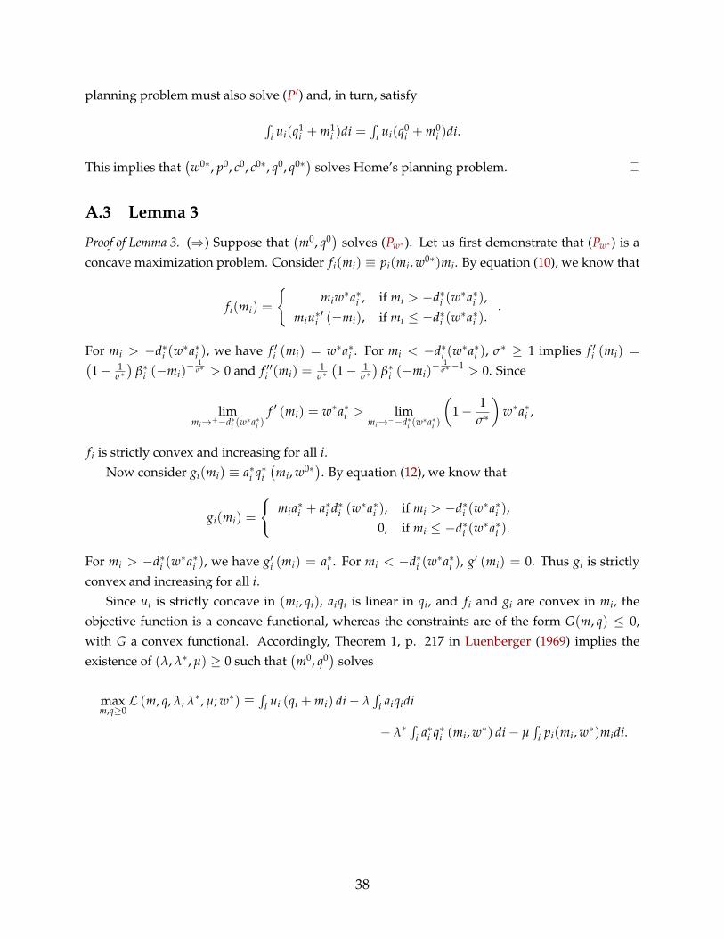
planning problem must also solve (P′) and, in turn, satisfy
´i ui(q1
i + m1i )di =
´i ui(q0
i + m0i )di.
This implies that(w0∗, p0, c0, c0∗, q0, q0∗) solves Home’s planning problem.
A.3 Lemma 3
Proof of Lemma 3. (⇒) Suppose that(m0, q0) solves (Pw∗). Let us first demonstrate that (Pw∗) is a
concave maximization problem. Consider fi(mi) ≡ pi(mi, w0∗)mi. By equation (10), we know that
fi(mi) =
{miw∗a∗i , if mi > −d∗i (w
∗a∗i ),miu∗′i (−mi), if mi ≤ −d∗i (w
∗a∗i )..
For mi > −d∗i (w∗a∗i ), we have f ′i (mi) = w∗a∗i . For mi < −d∗i (w
∗a∗i ), σ∗ ≥ 1 implies f ′i (mi) =(1− 1
σ∗)
β∗i (−mi)− 1
σ∗ > 0 and f ′′i (mi) =1
σ∗(1− 1
σ∗)
β∗i (−mi)− 1
σ∗−1 > 0. Since
limmi→+−d∗i (w
∗a∗i )f ′ (mi) = w∗a∗i > lim
mi→−−d∗i (w∗a∗i )
(1− 1
σ∗
)w∗a∗i ,
fi is strictly convex and increasing for all i.Now consider gi(mi) ≡ a∗i q∗i
(mi, w0∗). By equation (12), we know that
gi(mi) =
{mia∗i + a∗i d∗i (w
∗a∗i ), if mi > −d∗i (w∗a∗i ),
0, if mi ≤ −d∗i (w∗a∗i ).
For mi > −d∗i (w∗a∗i ), we have g′i (mi) = a∗i . For mi < −d∗i (w
∗a∗i ), g′ (mi) = 0. Thus gi is strictly
convex and increasing for all i.Since ui is strictly concave in (mi, qi), aiqi is linear in qi, and fi and gi are convex in mi, the
objective function is a concave functional, whereas the constraints are of the form G(m, q) ≤ 0,
with G a convex functional. Accordingly, Theorem 1, p. 217 in Luenberger (1969) implies the
existence of (λ, λ∗, µ) ≥ 0 such that(m0, q0) solves
maxm,q≥0
L (m, q, λ, λ∗, µ; w∗) ≡´
i ui (qi + mi) di− λ´
i aiqidi
− λ∗´
i a∗i q∗i (mi, w∗) di− µ´
i pi(mi, w∗)midi.
38

and the three following conditions hold:
λ(
L− ´i aiq0i di)
= 0,
λ∗(
L∗ − ´i a∗i q∗i(m0
i , w∗)
di)
= 0,
µ(´
i pi(m0i , w∗)m0
i di)
= 0.
Since(m0, q0) satisfy constraints (15)-(17), we therefore have
λ ≥ 0,´
i aiq0i di ≤ L, with complementary slackness, (39)
λ∗ ≥ 0,´
i a∗i q∗i(m0
i , w∗)
di ≤ L∗, with complementary slackness, (40)
µ ≥ 0,´
i pi(mi, w∗)m0i di ≤ 0, with complementary slackness. (41)
To conclude, note that if(m0, q0) solves maxm,q≥0 L (m, q, λ, λ∗, µ; w∗), then for almost all i,
(m0
i , q0i
)must solve
maxmi ,qi≥0
Li (mi, qi, λ, λ∗, µ; w∗) ≡ ui (qi + mi)− λaiqi
− λ∗a∗i q∗i (mi, w∗)− µpi(mi, w∗)mi.
(⇐) Now suppose that(m0
i , q0i
)solves (Pi) for almost all i with λ, λ∗, µ such that conditions (39)-
(41) hold. This implies (m0, q0) ∈ arg max
m,q≥0L (m, q, λ, λ∗, µ; w∗) .
Suppose first that all Lagrange multipliers are strictly positive: λ > 0, λ∗ > 0, µ > 0, then
conditions (39)-(41) imply
´i aiq0
i di = L,´i a∗i q∗i
(m0
i , w∗)
di = L∗,´i pi(m0
i , w∗)m0i di = 0.
Thus Theorem 1, p. 220 in Luenberger (1969) immediately implies that(m0, q0) is a solution to
(Pw∗). Now suppose that at least one Lagrange multiplier is equal to zero. For expositional pur-
poses suppose that λ = 0, whereas λ∗ > 0 and µ > 0. In this case, we have
(m0, q0) ∈ arg max
m,q≥0L (m, q, 0, λ∗, µ; w∗)
and
´i a∗i q∗i
(m0
i , w∗)
di = L∗,´i pi(m0
i , w∗)m0i di = 0.
39

Thus Theorem 1, p. 220 in Luenberger (1969) now implies that(m0, q0) is a solution to
maxm,q≥0
´i ui (qi + mi) di
subject to
´i a∗i q∗i (mi, w∗) di ≤ L∗,´i mi pi(mi, w∗)di ≤ 0.
Since´
i aiq0i di ≤ L by condition (39),
(m0, q0) is therefore also a solution to (Pw∗). The other cases
can be dealt with in a similar manner.
40