comparative evaluation of various frequentist and bayesian ...€¦ · comput stat (2017) 32:1–33...
TRANSCRIPT

University of Groningen
Comparative evaluation of various frequentist and Bayesian non-homogeneous Poissoncounting modelsGrzegorczyk, Marco; Kamalabad, Mahdi Shafiee
Published in:Computational Statistics
DOI:10.1007/s00180-016-0686-y
IMPORTANT NOTE: You are advised to consult the publisher's version (publisher's PDF) if you wish to cite fromit. Please check the document version below.
Document VersionPublisher's PDF, also known as Version of record
Publication date:2017
Link to publication in University of Groningen/UMCG research database
Citation for published version (APA):Grzegorczyk, M., & Kamalabad, M. S. (2017). Comparative evaluation of various frequentist and Bayesiannon-homogeneous Poisson counting models. Computational Statistics, 32(1), 1-33.https://doi.org/10.1007/s00180-016-0686-y
CopyrightOther than for strictly personal use, it is not permitted to download or to forward/distribute the text or part of it without the consent of theauthor(s) and/or copyright holder(s), unless the work is under an open content license (like Creative Commons).
Take-down policyIf you believe that this document breaches copyright please contact us providing details, and we will remove access to the work immediatelyand investigate your claim.
Downloaded from the University of Groningen/UMCG research database (Pure): http://www.rug.nl/research/portal. For technical reasons thenumber of authors shown on this cover page is limited to 10 maximum.
Download date: 30-04-2020

Comput Stat (2017) 32:1–33DOI 10.1007/s00180-016-0686-y
ORIGINAL PAPER
Comparative evaluation of various frequentistand Bayesian non-homogeneous Poisson countingmodels
Marco Grzegorczyk1 · Mahdi Shafiee Kamalabad1
Received: 5 August 2015 / Accepted: 13 September 2016 / Published online: 5 October 2016© The Author(s) 2016. This article is published with open access at Springerlink.com
Abstract In this paper a comparative evaluation study on popular non-homogeneousPoisson models for count data is performed. For the study the standard homoge-neous Poisson model (HOM) and three non-homogeneous variants, namely a Poissonchangepoint model (CPS), a Poisson free mixture model (MIX), and a Poisson hiddenMarkov model (HMM) are implemented in both conceptual frameworks: a frequen-tist and a Bayesian framework. This yields eight models in total, and the goal of thepresented study is to shed some light onto their relative merits and shortcomings. Thefirst major objective is to cross-compare the performances of the four models (HOM,CPS, MIX and HMM) independently for both modelling frameworks (Bayesian andfrequentist). Subsequently, a pairwise comparison between the four Bayesian and thefour frequentist models is performed to elucidate to which extent the results of thetwo paradigms (‘Bayesian vs. frequentist’) differ. The evaluation study is performedon various synthetic Poisson data sets as well as on real-world taxi pick-up counts,extracted from the recently published New York City Taxi database.
Keywords Non-homogeneous count data · Mixture model · Changepoint model ·Hidden Markov model · Bayesian paradigm · Frequentist paradigm · New York CityTaxi data
Electronic supplementary material The online version of this article (doi:10.1007/s00180-016-0686-y)contains supplementary material, which is available to authorized users.
B Marco [email protected]
Mahdi Shafiee [email protected]
1 Johann Bernoulli Institute (JBI), Rijksuniversiteit Groningen, 9747 AG Groningen,The Netherlands
123

2 M. Grzegorczyk, M. Shafiee Kamalabad
1 Introduction
The Poisson distribution is one of the most popular statistical standard tools foranalysing (homogeneous) count data, i.e. integer-valued samples. For modelling non-homogeneous count data, e.g. time series where the number of counts depends ontime and hence systematically differs over time, various extensions of the standardPoisson model have been proposed and applied in the literature. More appropri-ate non-homogeneous Poisson models can be easily obtained by embedding thestandard Poisson model into other statistical frameworks, such as changepoint mod-els (CPS), finite mixture models (MIX), or hidden Markov models (HMM). Thethree aforementioned modelling approaches have become very popular statisticaltools throughout the years for the following three reasons: (i) First, each of thethree modelling approaches is of a generic nature so that it can be combined witha huge variety of statistical distributions and models to extend their flexibilities.(ii) Second, the statistical methodology behind those generic models is rather sim-ple, described in lots of textbooks on Statistics and the model inference is feasible.(iii) Third, the three approaches can be easily formulated and implemented in bothconceptual frameworks: the standard ‘frequentist’ framework and the Bayesian frame-work.
Despite this popularity, the performances of the resulting non-homogeneousmodelshave never been systematically compared with each other in the statistical literature.This paper tries to fill this gap and presents a comparative evaluation study on non-homogeneous Poisson count data, for which those three well-known statistical models(changepoint models, mixturemodels and hiddenMarkovmodels) are implemented inboth conceptual frameworks: the frequentist framework and the Bayesian framework.
More precisely, for the evaluation study the standard homogeneous Poisson model(HOM) and three non-homogeneous variants thereof, namely a Poisson change-point model (CPS), a Poisson free mixture model (MIX), and a Poisson hiddenMarkov model (HMM) are implemented in a frequentist as well as in a Bayesianframework. The goal of the presented study is to systematically cross-comparethe performances. Thereby the focus is not only on cross-comparing the genericmodelling approach for non-homogeneity (CPS, MIX and HMM), but also oncomparing the frequentist model instantiations with the Bayesian model instan-tiations. The study is performed on various synthetic data sets as well as onreal-world taxi pick-up counts, extracted from the recently published New YorkCity Taxi (NYCT) database. In all presented applications it is assumed that thePoisson parameter does not depend on any external covariates so that the changesare time-effects only. That is, the non-stationarity is implemented intrinsically bytemporal changepoints, at which the Poisson process spontaneously changes its val-ues.
Within this introductory text no literature references have been given, since detaileddescriptions of all those generic statistical concepts, mentioned so far, can be found inmany standard textbooks on Statistics, and therefore, in principle, will be familiar formost of the readers. However, in Sect. 2, where the models are described and math-ematically formulated, explicit literature references will be provided for all modelsunder comparison.
123

Comparative evaluation of Poisson counting models 3
2 Methodology
2.1 Mathematical notations
Let D denote a n-by-T data matrix, whose columns refer to equidistant time points,t ∈ {1, . . . , T }, and whose rows refer to independent counts, i ∈ {1, . . . , n}, whichwere observed at the corresponding time points. The element di,t in the ith row andtth column of D is the ith count, which was observed at the tth time point. Let D.,t :=(d1,t , . . . , dn,t )
T denote the t th column of D, where “T” denotes vector transposition.D.,t is then the vector of the n observed counts for time point t .
Assume that the time points 1, . . . , T are linked to K Poisson distributions withparameters θ1, . . . , θK . The T time points can then be assigned to K components,which represent the K Poisson distributions. More formally, let the allocation vectorV = (v1, . . . , vT )T define an allocation of the time points to components, wherecomponent k represents a Poisson distribution with parameter θk . vt = k means thattime point t is allocated to the kth component and that the observations at t stem froma Poisson distribution with parameter θk (t = 1, . . . , T and k = 1, . . . , K ). Notethat the n independent counts within each column are always allocated to the samecomponent, while the T columns (time points) are allocated to different components.Define D[k] to be the sub-matrix, containing only the columns of D that are allocatedto component k.
The probability density function (pdf) of a Poisson distribution with parameterθ > 0 is:
p(x |θ) = θ x · exp{−θ}x ! (1)
for x ∈ N0. Assuming that all counts, allocated to k, are realisations of independentlyand identically distributed (iid) Poisson variables with parameter θk , the joint pdf isgiven by:
p(D[k]|θk) =T∏
t=1
I{vt =k}(t) · p(D.,t |θk) (2)
where I{vt =k}(t) indicates whether time point t is allocated to component k, and
p(D.,t |θk) =n∏
i=1
p(di,t |θk) = (θk){∑n
i=1 di,t } · exp{−n · θk}d1,t ! · . . . · dn,t ! (3)
is the joint pdf of the counts in the t th column of D. Given the allocation vectorV, which allocates the data into K sub-matrices D[1], . . . ,D[K ], and independentcomponent-specific Poisson distributions with parameters θ1, . . . , θK , the joint pdf ofD is:
p(D|V, θ) =K∏
k=1
p(D[k]|θk) (4)
where θ := (θ1, . . . , θK )T, and p(D[k]|θk) was defined in Eq. (2).
123

4 M. Grzegorczyk, M. Shafiee Kamalabad
Now assume that the allocation vectorV is known and fixed, while the component-specific Poisson parameters are unknown and have to be inferred from the data D.
Following the frequentist paradigm, the parameters can be estimated by theMaximum Likelihood (ML) approach. The ML estimators which maximise the log-likelihood
l(θ |V,D) := log{p(D|V, θ)} (5)
are given by θ = (θ1, . . . , θK )T, where θk is the empirical mean of all counts in D[k].Assuming that Tk time points are allocated to component k, the matrix D[k] containsTk · n counts and
θk = 1
n · Tk
T∑
t=1
I{vt =k}(t)n∑
i=1
di,t (6)
In a Bayesian setting the Poisson parameters in θ are assumed to be random variablesas well, and prior distributions are imposed on them. The standard conjugate prior fora Poisson model with parameter θk > 0 is the Gamma distribution:
p(θk |a, b) = ba
�(a)· (θk)
a−1 exp{−θk · b} (7)
where a is the shape and b is the rate parameter. Due to standard conjugacy argu-ments, for each component k the posterior distribution is a Gamma distribution withparameters a = a + ξ [k] and b = b + n · Tk
p(θk |D[k]) = (b + n · Tk)a+ξ [k]
�(a + ξ [k])· (θk)
a+ξ [k]−1 exp{−θk · (b + n · Tk)} (8)
where ξ [k] is the sum of all n · TK elements of the n-by-Tk (sub-)matrix D[k]. Themarginal likelihood can be computed in closed-form:
p(D[k]|a, b) =∫ ∞
0p(D[k]|θk)p(θk |a, b)dθk
= ba
�(a)· 1∏Tk
t=1
∏ni=1(d
[k]i,t )! · �(a + ξ [k])
(Tk · n + b)ξ[k]+a
(9)
where d[k]i,t is the element in the i th row and t th column of D[k].
Imposing independent Gamma priors on each component k ∈ {1 . . . , K } inducedby the allocation vector V, the marginal likelihood for the complete data matrix D is:
p(D|V) =K∏
k=1
p(D[k]|a, b) (10)
where the dependence on the fixed hyperparameters a and b on the left hand side ofthe last equation was suppressed.
123

Comparative evaluation of Poisson counting models 5
So far it has been assumed that the allocation vectorV is known and fixed, althoughV will be unknown for many real-world applications so that V also has to be inferredfrom the data D. The next section is therefore on the allocation vector inference.
2.2 Allocation vector inference
The standard frequentist Poisson or Bayesian Poisson–Gamma model assumes thatthe data are homogeneous so that all time points t = 1, . . . , T always belong to thesame component; i.e. K = 1 and V = (1, . . . , 1)T. These models are referred to asthe homogeneous (HOM) models. The HOM model is not adequate if the numberof counts varies over time, and non-homogeneous Poisson models, which infer theunderlying allocation, have to be used instead. Prominent approaches to model non-homogeneity include: multiple changepoint processes (CPS), finite mixture models(MIX), and hidden Markov models (HMM). CPS impose a set of changepoints whichdivide the time series 1, . . . , T into disjunct segments. Although this is a very naturalchoice for temporal data, the disadvantage is that the allocation space is restricted,as data points in different segments cannot be allocated to the same component; i.e.a component once left cannot be revisited. E.g. for T = 6 the true allocation V =(1, 1, 2, 2, 2, 1)T cannot be modelled and the best CPS model approximation mightbe: VC P S = (1, 1, 2, 2, 2, 3)T. The MIX model, on the other hand, is more flexible,as it allows for a free allocation of the time points so thatV is part of the configurationspace. But MIX does not take the temporal ordering of the data points into account. Ittreats the T time points as interchangeable units. This implies in the example abovethat all allocation vectors, which allocate T1 = 3 time points to component k = 1and T2 = 3 time points to component k = 2, are always equally supported a priori;including unlikely allocations, such as: V� = (1, 2, 1, 2, 1, 2)T.
A compromise between CPS andMIX is the hiddenMarkov model (HMM). HMMallows for an unrestricted allocation vector configuration space, but unlikeMIX it doesnot ignore the order of the time points. A homogeneous first-order HMM imposes a(homogeneous) Markovian dependency among the components v1, . . . , vT of V sothat the value of vt depends on the value of the preceding time point vt−1, and thehomogeneous state-transition probabilities can be such that neighbouring points arelikely to be allocated to the same component, while components once left can berevisited. The aforementioned Poisson models, can be implemented in a frequentistas well as in a Bayesian framework, yielding 8 non-homogeneous Poisson models intotal, see Table 1 for an overview.
2.3 The frequentist framework
The learning algorithms for the non-homogeneous frequentist models learn the best-fittingmodel for each number of components K , and the goodness of fit increases in K .Restricting K to be in between 1 and KM AX , for each approach (CPS,MIX andHMM)the best fitting model with K components, symbolically MK , can be learnt from thedata D. The Bayesian Information criterion (BIC), proposed by Schwarz (1978), is awell-known model selection criterion and balances between the goodness of fit and
123

6 M. Grzegorczyk, M. Shafiee Kamalabad
Table1
Overviewto
theeigh
t(no
n-)hom
ogeneous
Poissonmod
elsun
dercomparison
Frequentistv
ersion
(FREQ)
Bayesianversion(BAYES)
Hom
ogeneous
mod
el(H
OM)
with
1parameter
SeeSect.2
.3.1.W
ell-kn
ownstandard
mod
elfrom
frequentisttextboo
kswith
closed-form
solutio
nSeeSect.2.4.1.W
ell-kn
ownstandard
mod
elfrom
Bayesiantextbo
okswith
closed-form
solutio
n
Chang
epoint
mod
el(C
PS)with
Kparameters
SeeSect.2
.3.2.F
oreach
Kthebestchangepointsetcan
bedeterm
ined
with
theSegm
entN
eigh
bourho
odSearch
Algorith
m.B
ICisused
formodelselection
SeeSect.2.4.2.M
odelaveragingviaMCMC,based
onchangepo
intb
irth,death,and
reallocatio
nmoves
Finitemixture
model(M
IX)with
2K
−1parameters
SeeSect.2
.3.3.F
oreach
K,the
MLestim
atorsof
the
incompletemod
elcanbe
inferred
with
theEM
algo
rithm.B
ICisused
formod
elselection
SeeSect.2.4.3.M
odelaveragingviaMCMC,based
onthemoves
oftheallocatio
nsampler
HiddenMarkovmodel(H
MM)
with
K2
+2
K−
1parameters
SeeSect.2
.3.4.F
oreach
K,the
MLestim
atorsof
the
incompletemod
elcanbe
inferred
with
theEM
algo
rithm.B
ICisused
formod
elselection
SeeSect.2.4.4.M
odelaveragingviaMCMC,based
onthemoves
oftheallocatio
nsampler
andfour
additio
nalm
oves
Detailedexplanations
aregivenin
themaintext
123

Comparative evaluation of Poisson counting models 7
model sparsity. According to the BIC, among a set of models {M1, . . . ,MKM AX }, theone with the lowest BIC value is considered the most appropriate one with the besttrade-off (fit vs. sparsity). Given the n-by-T data set matrix D, and modelsMK withK components and qMK parameters (K = 1, . . . , KM AX ), the BIC ofMK is definedas
B I C(MK ) = −2 · log{p(D|MK )} + qMK · log(n · T ) (11)
where n · T is the number of data points in D, and for K = 1 each of the threenon-homogeneous model becomes the homogeneous modelM1 (see Sect. 2.3.1).
2.3.1 The homogeneous frequentist Poisson model (FREQ–HOM)
The homogeneous model M1 assumes that the counts stay constant over time, i.e.that there is only one single component, K = 1, and that the allocation vectors assignall data points to this component, i.e. V = 1 = (1, . . . , 1)T. Hence, D[1] = D andaccording to Eq. (6), the maximum likelihood (ML) estimator of the single (qM1 = 1)Poisson parameter θ := θ1 is the empirical mean of all T · n data points in D.
2.3.2 The frequentist changepoint Poisson model (FREQ–CPS)
A changepoint model uses a changepoint set of K − 1 changepoints, C ={c1, . . . , cK−1}, where 1 < c1 < · · · < cK−1 < T , to divide the time points 1, . . . , Tinto K disjunct segments. Time point t is assigned to component k if ck−1 < t ≤ ck ,where c0 = 0 and cK = T are pseudo changepoints. This means for the t th element,vt , of the allocation vector,VC , implied by C : vt = k if ck−1 < t ≤ ck . A changepointset C with K − 1 changepoints implies a segmentation D[1], . . . ,D[K ] of the datamatrix D, and the ML estimators θk for the segment-specific Poisson parameters θk
can be computed with Eq. (6). The model fit can be quantified by plugging the MLestimators θ into the log-likelihood in Eq. (5):
l(θC |VC ,D) := log{p(D|VC , θC )} (12)
whereVC is the allocation vector implied byC , and θC is the vector ofML estimators.The best fitting set of K − 1 changepoints, C K , i.e. the set maximising Eq. (12), canbe found recursively by the segment neighbourhood search algorithm. This algorithm,proposed by Auger and Lawrence (1989), employs dynamic programming to findthe best fitting changepoint set with K − 1 changepoints for each K (2 ≤ K ≤KM AX ). The algorithm is outlined in Sect. 1 of the supplementary material. The bestchangepoint modelMK minimises the BIC in Eq. (11), and the output of the algorithm
is the corresponding allocation vector VC P S and the segment-specific ML-estimatorsθC P S := θ
C K .
2.3.3 The frequentist finite mixture Poisson model (FREQ–MIX)
In a frequentist finite mixture model with K components the time points 1, . . . , T aretreated as interchangeable units from amixture of K independent Poisson distributions
123
8 M. Grzegorczyk, M. Shafiee Kamalabad
with parameters θ1, . . . , θK and mixture weights π1, . . . , πK , where πk ≥ 0 for all k,and
∑Kk=1 πk = 1. The columns D.,t of the data matrix D are then considered as a
sample from this Poisson mixture distribution with pdf:
p(D.,t |θ ,π) =K∑
k=1
πk · p(D.,t |θk) (13)
where θ = (θ1, . . . , θK )T is the vector of Poisson parameters, π = (π1, . . . , πK )T
is the vector of mixture weights, and p(D.,t |θk) can be computed with Eq. (3). Themaximisation of Eq. (13) in the parameters (θ,π) is analytically not feasible so that theML estimates have to be determined numerically. For mixture distributions this can bedone with the Expectation Maximisation (EM) algorithm (Dempster et al. 1977). Themathematical details of the EM algorithm are provided in Sect. 2 of the supplementarymaterial. The best mixture model MK minimises the BIC in Eq. (11), where qK =K+(K−1) is the number of Poisson and (free)mixtureweight parameters.1 The outputof theEM-algorithm is thebest number of components KM I X , the correspondingT -by-KM I X allocation probability matrix �M I X , whose elements �t,k are the probabilitiesthat time point t belongs to component k, and the vector of ML estimators θ M I X .
2.3.4 The frequentist Hidden Markov Poisson model (FREQ–HMM)
The key assumption of a hidden Markov model (HMM) with K components (‘states’)is that the (unobserved) elements v1, . . . , vT of the allocation vector V follow a(homogeneous) first-order Markovian dependency. That is, {vt }t=1,...,T is considereda homogeneous Markov chain of order τ = 1 with the state space S = {1, . . . , K },the initial distribution = (π1, . . . , πK ), where πk ≥ 0 is the probability that v1is equal to k, and the K -by-K transition (probability) matrix A, whose elementsai, j ≥ 0 are the transition probabilities for a transition from state i to state j :ai, j = P(vt+1 = j |vt = i) for all t ∈ {1, . . . , T − 1}.2 Assume that there are Kstate-dependent Poisson distributions so that each state k ∈ {1, . . . , K } correspondsto a Poisson distribution with parameter θk . The data matrix D is then interpreted as asequence of its T columns,D.,1, . . . ,D.,T , and vt = k means that columnD.,t is a vec-tor of n realisations of the kth Poisson distribution with parameter θk . Mathematically,this means:
p(D.,t |vt = k) = p(D.,t |θk) (14)
where p(D.,t |θk) was defined in Eq. (3). The Hidden Markov model is now fullyspecified and has the unknown parameters , A and θ = (θ1, . . . , θK )T. For givenparameters (,A, θ), the distribution of the unknown (‘hidden’) state sequencev1, . . . , vT can be inferred recursively with the foward and backward algorithm.And by combining the forward and backward algorithms with the EM algorithm,
1 The K mixture weights fulfil:∑K
k=1 πk = 1.2 It holds:
∑Kk=1 πk = 1, and
∑Kj=1 ai, j = 1 for all i .
123
Comparative evaluation of Poisson counting models 9
the best HMM model MK , which minimises the BIC in Eq. (11), can be numeri-cally determined. The details of the inference procedure are provided in Sect. 3 of thesupplementary material. For a HMM model with K components the total number ofparameters is qK = K+ (K− 1) + (K2 −K), i.e. the sum of the Poisson parameters,the free initial probability parameters and the free transition probability parameters.3
The output of the EM algorithm, as described in Sect. 3 of the supplementary paper,is the best number of components K H M M , the corresponding T -by-K H M M allocationprobability matrix �H M M , whose elements �t,k are the probabilities that time pointt belongs to component k, and the ML-estimators θ H M M .
2.4 The Bayesian framework
The Bayesian models employ a Poisson-Gamma model, for which the marginal like-lihood p(D|V) can be computed with Eq. (10). While the homogeneous model,described in Sect. 2.4.1, keeps K = 1 fixed, the three non-homogeneous models haveto infer K and the unknown allocation vector V. In a Bayesian framework this meansthat prior distributions have to be imposed on V and K . The three non-homogeneousmodels, described below, assume that the joint prior distribution can be factorized,p(V, K ) = p(V|K ) · p(K ), and impose on K a truncated Poisson distribution withparameterλ and the truncation 1 ≤ K ≤ KM AX so that p(K ) ∝ λK ·exp{−λ}·(K !)−1.
Subsequently, the prior onV is specified conditional on K . The marginal likelihoodp(D|V) and the two prior distributions p(K ) and p(V|K ) together fully specify theBayesian model, and Markov Chain Monte Carlo (MCMC) simulations are used togenerate samples (V(1), K (1)), . . . , (V(R), K (R)) from the posterior distribution:
p(V, K |D) ∝ p(D|V) · p(V|K )p(K ) (15)
The Bayesian models, described below, differ only by the conditional prior p(V|K ).
2.4.1 The homogeneous Bayesian Poisson–Gamma model (BAYES–HOM)
The homogeneous Bayesian model assumes that the counts do not vary over time, sothat K = 1 and V = (1, . . . , 1)T =: 1 and D[1] = D. According to Eqs. (9–10), themarginal likelihood of the BAYES–HOM model is then given by
p(D[1]|V = 1) =∫ ∞
0p(D|θ)p(θ |a, b)dθ
= ba
�(a)· 1∏T
t=1∏n
i=1(di,t )!· �(a + ξ)
(T · n + b)ξ+a
where di,t is the element in the i th row and t th column of D, and ξ is the sum of alln · T elements of D.
3 Note that:∑K
k=1 πk = 1, and∑K
l=1 ak,l = 1 for k = 1, . . . , K .
123

10 M. Grzegorczyk, M. Shafiee Kamalabad
2.4.2 The Bayesian changepoint Poisson–Gamma model (BAYES–CPS)
There are various possibilities to implement a Bayesian changepoint model, and herethe classical one from Green (1995) is used. The prior on K is a truncated Poissondistribution, and each K is identifiedwith K −1 changepoints c1, . . . , cK−1 on the dis-crete set {1, . . . , T − 1}, where vt = k if ck−1 < t ≤ ck , and c0 := 1 and cK := T arepseudo changepoints. Conditional on K , the changepoints are assumed to be distrib-uted like the even-numbered order statistics of L := 2(K −1)+1 points uniformly andindependently distributed on {1, . . . , T − 1}. This implies that changepoints cannotbe located at neighbouring time points and induces the prior distribution:
P(V|K ) = 1(T − 1
2(K − 1) + 1
)K−1∏
k=0
(ck+1 − ck − 1) (16)
The BAYES–CPS model is now fully specified and K and V can be sampled fromthe posterior distribution p(V, K |D), defined in Eq. (15), with a Metropolis-HastingsMCMC sampling scheme, based on changepoint birth, death and re-allocation moves(Green 1995).
Given the current state at the r th MCMC iteration: (V(r), K (r)), where V(r) can beidentified with the changepoint set: C (r) = {c1, . . . , cK (r)−1}, one of the three movetypes is randomly selected (e.g. each with probability 1/3) and performed. The threemove types (i–iii) can be briefly described as follows:
(i) In the changepoint reallocation move one changepoint c j from the currentchangepoint set C (r) is randomly selected, and the replacement changepoint israndomlydrawn from the set
{c j−1 + 2, . . . , c j+1 − 2
}. ThenewsetC� gives the
new candidate allocation vectorV�; the number of components stays unchanged:K � = K (r).
(ii) The changepoint birth move randomly draws the location of one single newchangepoint from the set of all valid new changepoint locations:
B† :={
c ∈ {1, . . . , T − 1} : |c − c j | > 1∀ j ∈{1, . . . , K (r) − 1
}}(17)
Adding the new changepoint to C (r) yields K � = K (r) + 1, and the new set C�,which yields the new allocation vector V�.
(iii) The changepoint death move is complementary to the birth move. It randomlyselects one of the changepoints from C (r) and proposes to delete it. This givesthe new changepoint set C� which yields the new candidate allocation vectorV�, and K � = K (r) − 1.For all three moves the Metropolis-Hastings acceptance probability for the newcandidate state (V�, K �) is given by A = min{1, R}, with
R = p(D|V�)
p(D|V(r))· p(V�|K �)p(K �)
p(V(r)|K (r))p(K (r))· Q (18)
123

Comparative evaluation of Poisson counting models 11
where Q is the Hastings ratio, which can be computed straightforwardly foreach of the three move types (see, e.g., Green (1995)). If the move is accepted,set V(r+1) = V� and K (r+1) = K �, or otherwise leave the state unchanged:V(r+1) = V(r) and K (r+1) = K (r).
2.4.3 The Bayesian finite mixture Poisson–Gamma model (BAYES–MIX)
Here, the Bayesian finite mixture model instantiation and the Metropolis HastingsMCMC sampling scheme proposed by Nobile and Fearnside (2007) is employed.The prior on K is a truncated Poisson distribution, and conditional on K , a categoricaldistribution (with K categories) and probability parametersp = (p1, . . . , pK )T is usedas prior for the allocation variables v1, . . . , vT ∈ {1, . . . , K }. That is, ∑K
k=1 pk = 1and p(vt = k) = pk . The probability of the allocation vector V = (v1, . . . , vT )T isthen given by:
p(V|p) =K∏
k=1
(pk)nk (19)
where nk = |{t ∈ {1, . . . , T } : vt = k}| is the number of time points that are allocatedto component k by V. Imposing a conjugate Dirichlet distribution with parametersα = (α1, . . . , αK )T on p and marginalizing over p, yields the closed-form solution:
p(V|K ) =∫
p(V|p)p(p|α)dp = �(∑K
k=1 αk)
�(∑K
k=1(nk + αk))
K∏
k=1
�(nk + αk)
�(αk)(20)
The BAYES–MIXmodel is now fully specified, and the posterior distribution is invari-ant to permutations of the components’ labels if: αk = α. A Metropolis-HastingsMCMC sampling scheme, proposed by Nobile and Fearnside (2007) and referred toas the “allocation sampler”, can be used to generate a sample from the posterior dis-tribution in Eq. (15). The allocation sampler consists of a simple Gibbs move and fivemore involved Metropolis-Hastings moves. Given the current state at the r th iteration:(V(r), K (r)) the Gibbs move keeps the number of components fixed, K (r+1) = K (r),and just re-samples the value of one single allocation variable v
(r)t from its full con-
ditional distribution. This yields a new allocation vector V(r+1) with a re-sampled t thcomponent v(r+1)
t . As this Gibbs move has two disadvantages, Nobile and Fearnside(2007) propose to use five additional Metropolis Hastings MCMC moves. (i) As theGibbs move yields only very small steps in the allocation vector configuration space,Nobile and Fearnside (2007) propose three additional Metropolis Hastings MCMCmoves, referred to as the M1, M2 and M3 move, which also keep K (r) fixed but allowfor re-allocations of larger sub-sets of the allocation variables v
(r)1 , . . . , v
(r)T . (ii) As
neither the Gibbs move nor the M1-M3moves can change the number of components,Nobile and Fearnside (2007) also propose a pair of moves, referred to as the Ejection-and Absorption move, which generate a new or delete an existing component, so thatK (r+1) = K (r) + 1 or K (r+1) = K (r) − 1, respectively. The technical details of themoves can be found in Nobile and Fearnside (2007).
123

12 M. Grzegorczyk, M. Shafiee Kamalabad
2.4.4 The Bayesian hidden Markov Poisson–Gamma model (BAYES–HMM)
The focus is on aBayesian hiddenMarkovmodel instantiation,whichwas recently pro-posed in Grzegorczyk (2016) in the context of non-homogeneous dynamic Bayesiannetwork models. The prior on K follows a truncated Poisson distribution, and for eachK a HMM model with K states is used to model the allocation vector V. To this end,V is identified with the temporally ordered sequence of its components: v1, . . . , vT ,and it is assumed that the latter sequence describes a homogeneous first order Markovchain with a uniform initial distribution and a K -by-K transition matrix A.
Let al,k be the element in the lth row and kth column of the transition matrixA. al,k is then the probability for a transition from component l to component k,and
∑Kk=1 al,k = 1. For a homogeneous Markov chain this means: al,k = P(vt =
k|vt−1 = l,A, K ) for all t , and hence:
p(V|A, K ) = p(v1, . . . , vT |A, K ) = p(v1|K )
T∏
t=2
p(vt |vt−1,A, K )
= 1
K
K∏
k=1
K∏
l=1
(al,k
)nl,k (21)
where nl,k = |{t ∈ {2, . . . , T } : vt = k ∧ vt−1 = l}| is the number of transitions froml to k in the sequence v1, . . . , vT .
Each rowAl,. of the transitionmatrixAdefines the probability vector of a categoricalrandom variable (with K categories), and on each vectorAl,. an independent Dirichletprior with parameter vector αl = (αl,1, . . . , αl,K )T can be imposed:
p(Al,.|αl) =∏K
k=1 �(αl,k)
�(∑K
k=1 αl,k)
K∏
k=1
(al,k
)αl,k−1 (22)
Marginalizing over the transition matrix A in Eq. (21), i.e. marginalizing over therow vectors A1,., . . . ,AK ,., where each row vector Al,. has an independent Dirichletprior, defined in Eq. (22), gives the marginal distribution:
p(V|K ) =∫
A1,.
. . .
∫
AK ,.
p(V|A, K )
{K∏
l=1
p(Al,.|αl)
}dA1,. . . . dAK ,. (23)
Inserting Eq. (21) into Eq. (23) yields:
P(V|K ) = 1
K
K∏
l=1
(∫
Al,.
P(Al,.|αl)
K∏
k=1
(al,k
)nl,k dAl,.
)(24)
The inner integrals in Eq. (23) correspond to Multinomial-Dirichlet distributions,which can be computed in closed form:
123

Comparative evaluation of Poisson counting models 13
P(V|K ) = 1
K
K∏
l=1
�(∑K
k=1 αl,k)
�(∑K
k=1 nl,k + αl,k)
K∏
k=1
�(nl,k + αl,k)
�(αl,k)(25)
The BAYES–HMM model is now fully specified, and with αl,k = α in Eq. (22) themarginal distribution P(V|K ) in Eq. (25) is invariant to permutations of the states’labels.
In principle, the allocation sampler from Nobile and Fearnside (2007) fromSect. 2.4.3 can also be used to generate a sample from the posterior distribution inEq. (15). However, the allocation sampler moves have been developed for finite mix-ture models, where data points are treated as interchangeable units without any order.Hence, the allocation sampler moves are sub-optimal when a Markovian dependencystructure among temporal data points is given. In Grzegorczyk (2016) it has beenshown that the performance of the allocation sampler can be significantly improvedin terms of convergence and mixing by including two new pairs of complementaryMetropolis-Hastings moves. These two pairs of moves, referred to as the ‘inclusionand exclusion moves’ and the ‘birth and death moves’ in Grzegorczyk (2016), exploitthe temporal structure of the data points. A detailed description of these moves can befound in Grzegorczyk (2016).
3 Validation
Table 1 gives an overview to the models from Sect. 2, and Table 2 shows the outputsof those models. The outputs range from a scalar ML estimate (FREQ–HOM) to anMCMC sample of allocation vectors (e.g. BAYES–HMM). For each model the outputinferred from D can be used to estimate the probability of a new validation data set D.Assume that in addition to the n-by-T data matrix D from Sect. 2.1, another n-by-Tdata matrix D is given and that the time points 1, . . . , T in D and D can be mappedonto each other.
Each non-homogeneousBayesianmodelwith K components and allocation vectorV inferred fromD can then be used to subdivide the newdatamatrix D into submatricesD[1], . . . , D[K ], and the predictive probability for the kth sub-matrix D[k] is:
p(D[k]|D[k]) =∫ ∞
0p(D[k]|θk)p(θk |D[k])dθk
= ba
�(a)· 1∏Tk
t=1
∏ni=1(d
[k]i,t )! · �(a + ξ [k])
(Tk · n + b)ξ[k]+a
(26)
where Tk is the number of columns allocated to k, a = a + ξ [k] and b = b + n · Tk arethe posterior parameters, defined above Eq. (8), ξ [k] is the sum of all n · Tk elementsof the n-by-Tk sub-matrix D[k], and d[k]
i,t is the element in the i th row and t th column
of D[k].
123

14 M. Grzegorczyk, M. Shafiee Kamalabad
Table2
Overviewof
theou
tputsof
theeigh
t(no
n-)hom
ogeneous
Poissonmod
els
Frequentistv
ersion
(FREQ)
Bayesianversion(BAYES)
Hom
ogeneous
mod
el(H
OM)
with
1parameter
K=
1,V
=(1
,..
.,1)
Tscalar
ML-estim
ator
θ
estim
ated
from
the
n-by
-Tvalues
inD
K=
1,V
=(1
,..
.,1)
T1-dimension
alpo
sterior
distributio
np(
θ|D
)inferred
from
the
n-by
-Tvalues
inD
Chang
epoint
mod
el(C
PS)with
Kparameters
KC
PS,o
neco
ncre
teallocatio
nvector
instantiatio
nV
CP
S,and
avector
ofthe
KC
PScomponent-specific
ML-estim
atorsθ
CP
S
Asample
{K(r
) ,V
(r) } r
=1,...,R,and
foreach
raseto
fK
(r)posteriordistributio
nsp(
θ k,r
|D[k,
r] )where
θ k,r
and
D[k,
r]referto
the
kthcompo
nent
ofthe
rth
sample
Finitemixture
model(M
IX)with
2K
−1parameters
KM
IX,a
vector
oftheK
MIX
component-specific
ML
estim
atorsθ
MIX
,and
aT-by-
Kmatrix
�M
IX,whose
elem
ents
�t,
karetheestim
ated
allocatio
nprobabilities
p(v
t=
k|D)
Asample
{K(r
) ,V
(r) } r
=1,...,R,and
foreach
raseto
fK
(r)posteriordistributio
nsp(
θ k,r
|D[k,
r] )where
θ k,r
and
D[k,
r]referto
the
kthcompo
nent
ofthe
rth
sample
HiddenMarkovmodel(H
MM)
with
K2
+2
K−
1parameters
K,a
vector
ofthe
KH
MM
component-specific
ML
estim
atorsθ
HM
M,and
aT-by-
Kmatrix
�H
MM
whose
elem
ents
�t,
karetheestim
ated
allocatio
nprobabilities
p(v
t=
k|D)
Asample
{K(r
) ,V
(r) } r
=1,...,R,and
foreach
raseto
fK
(r)posteriordistributio
nsp(
θ k,r
|D[k,
r] )where
θ k,r
and
D[k,
r]referto
the
kthcompo
nent
ofthe
rth
sample
Detailedexplanations
aregivenin
themaintext
123

Comparative evaluation of Poisson counting models 15
The (logarithmic) predictive probability of D conditional on K and V is then givenby:
log{p(D|D,V, K )} =K∑
k=1
log{p(D[k]|D[k])} (27)
For the homogeneous Bayesian model with K = 1, D[1] = D, and D[1] = D, thepredictive probability of D can be computed analytically. For each non-homogeneousBayesian model M an MCMC simulation generates a sample {V(r), K (r)}r=1,...,R
from the posterior distribution p(K ,V|D) in Eq. (15), and the predictive probabilityof model M can be approximated by:
log{p(D|D,M)} ≈ 1
R
R∑
r=1
log{p(D|D,V(r), K (r))} (28)
For the frequentist models it can be proceeded similarly: After data matrix D hasbeen used to learn a model and its ML-estimates, the probability of the new datamatrix D, given the model and the ML estimates learnt from D, is a measure whichcorresponds to a Bayesian predictive probability. The homogeneous model and thechangepoint model both output concrete values for K and V, and:
log{p(D|K , V, θ)} =K∑
k=1
log{p(D[k,V]|θk)} (29)
where K , V, and θ are those values inferred from the training data D, D[k,V] is the kth
submatrix of the validation data D implied by V, and p(D[k,V]|θk) can be computedwith Eq. (2).4 FREQ–MIX and FREQ–HMM both infer the number of components Kand the Poisson parameters θ but no concrete allocation vector. They infer a K -by-Tmatrix �, whose elements �k,t are the probabilities that time point t is allocated tocomponent k, symbolically �k,t = p(vt = k|D). The probability of the new data setD is then given by:
log{p(D|K , �, θ)}T∑
t=1
log{K∑
k=1
�k,t · p(D.,t |θk)} (30)
4 Data
4.1 Synthetic data
Synthetic count data matrices are generated as follows: letV� = (v�1, . . . , v
�T )T be the
true allocation vector, which allocates each time point t ∈ {1, . . . , T } to a component
4 For the homogeneous model it holds: K = 1 and D[1,V] = D.
123

16 M. Grzegorczyk, M. Shafiee Kamalabad
k ∈ {1, . . . , K �}, where v�t = k means that t is allocated to k. Given V�, n-by-T data
set matrices D� can be obtained by sampling each matrix element d�i,t independently
from a Poisson distribution with parameter θv�t(i = 1, . . . , n and t = 1, . . . , T ).
The focus of the study is on different allocation vectors V� with differentcomponent-specific Poisson parameters θ1, . . . , θK � . Let P� = (p1, . . . , pT ) denote arow vector whose element pt is the Poisson parameter for time point t . That is, pt = λ
means that V� allocates time point t to a component with Poisson parameter θv�t
= λ.The row vector P� will be referred to as the vector of Poisson parameters.
Let sm denote a row vector of length m, whose elements are all equal to s ∈ N,sm = (s, . . . , s). The situation, where an allocation vectorV� allocates T = 4 ·m timepoints to K � = 4 equidistant coherent segments of lengthm, with the four component-specific Poisson parameters θ1 = 1, θ2 = 5, θ3 = 3, and θ4 = 8, can then be definedcompactly:
P� = (1, . . . , 1︸ ︷︷ ︸m−times
, 5, . . . , 5︸ ︷︷ ︸m−times
, 3, . . . , 3︸ ︷︷ ︸m−times
, 8, . . . , 8︸ ︷︷ ︸m−times
) =: (1m, 5m, 3m, 8m)
For the situation where the allocation vector follows a free mixture model, e.g., byallocating T = 2 · m time points to K � = 2 components with Poisson parametersθ1 = 1 and θ2 = 5, let P� = MIX(1m, 5m) denote that P� is a row vector whoseelements are a random permutation of the elements of the vector (1m, 5m).
With regard to the real-world Taxi data, described in Sect. 4.2, each data matrix Dis built with T = 96 columns (time points) and n ∈ {1, 2, 4, 8, 16} rows (independentsamples per time point). An overview to the allocation schemes (vectors of Poissonparameters), employed in the comparative evaluation study, is given in Table 4 of thesupplementary material. For each of the four allocation scenarios (HOM, CPS, MIX,and HMM) two different vectors of Poisson parameters are considered. Data matricesare built with a varying no. of rows n ∈ {1, 2, 4, 8, 16} and T = 96 columns. For eachof the resulting 4 · 2 · 5 = 40 combinations, 25 independent data matrix instantiationsare generated, i.e. 1000 data matrices in total. Subsequently, for each of those 1000data matrix instantiations a n-by-T validation data matrix with n = 30 and T = 96 issampled the same way (using the same vector of Poisson parameters).5
4.2 The New York City Taxi (NYCT) data from 2013
Through a ‘Freedom of Information Law’ request from the ‘New York City Taxi andLimousine Commission’ a dataset, covering information of about 700 million taxitrips in New York City (USA) from the calendar years 2010–2013, was published andstored by the University of Illinois (Donovan andWork 2015). In the NYCT database,for each trip various details are provided; e.g. (i) the number of transported passengers,(ii) the pick-up and drop-off dates and daytimes, (iii) the GPS coordinates, where thepassenger(s) were picked up and dropped off.6 In this paper the focus is on the pick-up
5 Note that T and n have been set in accordance with the NYCT data, described in Sect. 4.2.6 The NYCT data can be downloaded from: http://dx.doi.org/10.13012/J8PN93H8
123

Comparative evaluation of Poisson counting models 17
daytime (discretised into 15min intervals)42812160
no. o
f pic
k-up
s
0
5
10
15 the first 4 Mondays in 2013
daytime (discretised into 15min intervals)42182190
no. o
f pic
k-up
s
0
5
10 averages per weekday in 2013
Fig. 1 NewYork City Taxi pick-up time series. To shed some light onto the variability of the daily profiles,the upper panel shows the time series of the first four Mondays in 2013. The lower panel shows the sevenweekday averages in 2013. Three weekdays with slightly deviating profiles have been highlighted: Sunday(bold black), Saturday (grey), and Friday (dotted black)
dates and daytimes of about 170 million taxi rides in the most recent year 2013, so thatonly a fractional amount of the data is used. Each pick-up is interpreted as a ‘taxi call’,so that it can be analysed how the number of taxi calls varies over the daytime. The datapreparation can be summarised as follows: For each of about 170 million taxi ridesfrom 2013 the pick-up date and daytime are extracted and down-sampled by a factorof 1000 (by randomly selecting 0.1% of the extracted samples), before all entriescorresponding to US holidays are withdrawn.7 Subsequently, there remain 169,596date-and-time entries, which subdivide onto the 7 weekdays as indicated in Table 5 ofthe supplementary material. Discretising the daytimes into T = 96 equidistant timeintervals,8 each covering 15min of the 24-h day, and binning the pick-up times ofeach individual day into the T = 96 time intervals, gives a 355-by-96 data matrix D,whose elements di,t are the number of taxi pick-ups (or taxi calls) on the i th day intime interval t . Since the seven weekdays might show different patterns, the data setmatrix D is subdivided into seven nw-by-T sub-matrices Dw (w = 1, . . . , 7), wherew indicates the weekday, and nw ∈ {46, 50, 51, 52} varies with the weekdays (seeTable 5 of the supplementary material). Figure 1 shows the number of Taxi calls forthe first four Mondays in 2013 and the weekday averages.
In the study theweekdays are analysed separately, as they are likely to showdifferentpatterns. For eachweekday n ∈ {1, 2, 4, 8, 16} rows (days) are randomly selected fromDw, before n = 30 of the remaining nw − n rows are randomly selected to build avalidation data matrix. Repeating this procedure 5-times independently yields 150data matrix pairs Dw,n,u and Dw,n,u , where w ∈ {1, . . . , 7} indicates the weekday,n ∈ {1, 2, 4, 8, 16} and n = 30 indicate the number of rows of Dw,n,u and Dw,n,u ,
7 The following US holidays in 2013 are excluded: Jan 1 (New Year’s Day), Jan 21 (Martin Luther King),Feb 18 (Presidents’ Day), May 27 (Memorial Day), Jul 4 (Independence Day), Sep 2 (Labor Day), Oct 14(Columbus Day), Nov 11 (Veterans Day), Nov 28 (Thanksgiving Day) and Dec 25 (Christmas Day).8 The time information is provided in seconds in the format: hh-mm-ss, ranging from 00-00-00 (midnight)to 23-59-59 (last second of the day).
123
18 M. Grzegorczyk, M. Shafiee Kamalabad
and u ∈ {1, . . . , 5} indicates the replicate. Each Dw,n,u is a n-by-96 matrix and eachDw,n,u is a 30-by-96 matrix.9
5 Simulation details
For all models the maximal number of components is set to KM AX = 10. In theGamma priors, see Eq. (7), both hyperparameters a and b are set to 1 so as toobtain rather uninformative priors. In terms of equivalent sample sizes this settingcorresponds to one (b = 1) additional pseudo observation with one single taxi call(a = 1) for each component. The hyperparameter of the truncated Poisson prioron the number of components of the non-homogeneous Bayesian models is set toλ = 1, meaning that a priori only one single component is expected (K = 1). Fur-thermore, all hyperparameters of the Dirichlet priors of the BAYES–MIX and theBAYES–HMM model are set to 1. That is, it was set α = 1 above Eq. (20) andαl = 1 (l = 1, . . . , K ) in Eq. (22). In terms of equivalent samples sizes this canbe interpreted as one pseudo count per mixture component (BAYES–MIX) or transi-tion (BAYES–HMM), respectively. The two homogeneous models (FREQ–HOM andBAYES–HOM) as well as the frequentist changepoint model (FREQ–CPS) alwaysoutput deterministic solutions. The EM-algorithm, which is used for inferring theFREQ–MIX and the FREQ–HMM model, can get stuck in local optima. Therefore,the EM algorithm is run 10 times independently for each data set with different ran-domly sampled initialisations of the Poisson parameters. ε = 0.001 is used for thestop-criterion (see Tables 1, 2 in the supplementary paper). For each K the outputwith the highest maximal likelihood value was selected, while the other EM algorithmoutputs were withdrawn.10 (The maximal likelihood value was typically reached sev-eral times, suggesting that running the EM algorithm 10 times is sufficient for theanalysed data.) The non-homogeneous Bayesian models are inferred with MCMCsimulations, and a pre-study was performed to determine the required number ofMCMC iterations. This pre-study was based on eight data sets with n = 16, onefrom each of the 8 allocation scenarios shown in Table 4 of the supplementary mate-rial. On each of these data sets 5 independent MCMC simulations with differentallocation vector initialisations were performed. Trace-plot diagnostics of the quan-tity: log(Likelihood)+log(Prior), which is proportional to the log posterior probability,as well as scatter plots of the pairwise co-allocation probabilities, p(vt1 = vt2 |D)
for t1, t2 ∈ {1, . . . , T }, indicated that the following MCMC simulation setting issufficient: The burn-in phase is set to 25,000 MCMC iterations, before R = 250equidistant samples are taken from the subsequent 25,000 MCMC iterations (sam-pling phase).
9 Note that the same number of validation samples (n = 30) is sampled for each n to ensure that thepredictive probabilities p(Dw,n,u |Dw,n,u) are comparable for different n.10 Note that the mixture weights and the transition probabilities were always initialised uniformly, i.e.πk = 1/K (FREQ–MIX) and ai, j = 1/K (FREQ–HMM).
123

Comparative evaluation of Poisson counting models 19
6 Comparative evaluation study
First, the synthetic data from Sect. 4.1 are analysed with the eight models listedin Tables 1, 2. The first finding is that the homogeneous models (FREQ–HOMand BAYES–HOM) yield substantially lower predictive probabilities than the non-homogeneous models for the non-homogeneous data. This is not unexpected, as thehomogeneous models can per se not deal with non-homogeneity (e.g. changepoint-segmented data). For clarity of the plots, the results of the homogeneous models aretherefore left out whenever their inclusion would have led to substantially differentscales.
Figures 2, 3 and 4 show histograms of the average log predictive probability differ-ences with separate histograms for the Bayesian and the frequentist models. Here, thefour models (HOM, CPS, MIX and HMM) are compared independently within theBayesian and within the frequentist framework without comparing the two paradigms(Bayesian vs. frequentist). In each histogram the models being most consistent withthe data (i.e. being most consistent with the data generation process), are used as ‘ref-erence’ models.11 In a complementary study the four Bayesian models and the fourfrequentist models are compared in a pairwise manner. In Figs. 5 and 6 for each ofthe four models (HOM, CPS, MIX and HMM) the average log predictive probabilitydifferences (‘Bayesian results minus frequentist results’) are plotted against the aver-age log predictive probability of the Bayesian and the frequentist results. The curves(‘differences vs. means’) are known as ‘Tukey mean-difference’ or ‘Bland-Altman’plots, see Cleveland (1994) or Bland and Altman (1995).
6.1 Global trends, Figs. 2–6
Before studying the individual results in more detail, two global trends become obvi-ous. Figures 2, 3 and 4 show that the predictive probability differences between thenon-homogeneous models get consistently lower as the number of samples n pertime point t increases. The only exception appears for the mixture data [panels (b)in Figs. 2, 3], as the changepoint models (BAYES–CPS and FREQ–CPS) can perse not deal with mixture allocations, even when the sample size n is large. That is,for sufficiently informative data each non-homogeneous model can approximate allkinds of non-homogeneity, unless there is a clear mismatch between the dependencystructure in the data and the inference model, as observed for the CPS models onmixture data. The second global finding from Figs. 5 and 6 is that the pairwise differ-ences between the Bayesian and the frequentist models consistently converge towardszero as the number of samples n increases. That is, asymptotically for all four mod-els the Bayesian variant and the frequentist variant perform equally well for all datascenarios.
11 For example the changepoint models (FREQ–CPS and BAYES–CPS) are used as references for the twochangepoint-segmented data scenarios: P� = (1m , 2m , 3m , 4m ) and P� = (1m , 2m , 3m , 4m , 5m , 6m ).
123

20 M. Grzegorczyk, M. Shafiee Kamalabad
BAYES n=1
-200
0
200
400
600
FREQ n=1
-200
0
200
400
600
BAYES n=2
0
100
200
FREQ n=2
0
100
200
BAYES n=4-20
0
20
40
60
80
FREQ n=4-20
0
20
40
60
80
BAYES n=80
10
20
30
FREQ n=80
10
20
30
BAYES n=160
2
4
6
8
FREQ n=160
2
4
6
8
(a)
BAYES n=1
0
1000
2000
FREQ n=1
0
1000
2000
BAYES n=2
0
500
1000
FREQ n=2
0
500
1000
BAYES n=40
100
200
300
400
FREQ n=40
100
200
300
400
BAYES n=8
0
50
100
150
200
FREQ n=8
0
50
100
150
200
BAYES n=160
50
100
FREQ n=160
50
100
(b)
(c)
BAYES n=1
0
500
1000
FREQ n=1
0
500
1000
BAYES n=20
100
200
300
FREQ n=20
100
200
300
BAYES n=40
10
20
30
40
FREQ n=40
10
20
30
40
BAYES n=8-2
0
2
4
6
FREQ n=8-2
0
2
4
6
BAYES n=16
0
0.5
1
1.5
2
2.5
FREQ n=16
0
0.5
1
1.5
2
2.5
Fig. 2 Cross-method comparison on synthetic data—part 1/3. a–c Histograms of the average log predic-tive probability differences for three non-homogeneous allocation scenarios with error bars representingstandard deviations. In each (a–c) the upper row refers to the Bayesian models while the bottom row refersto the frequentist models. In each panel the differences between the reference (=most consistent with thedata) model and the other two non-homogeneous models are shown. The homogeneous models led tosubstantially lower predictive probabilities and the results are therefore not shown. From left to right thesample size n increases and the scale of the y-axis changes. a Changepoint data P� = (1m , 2m , 3m , 4m ).LeftCPS–MIX, rightCPS–HMM. bMixture dataP� = M I X (1m , 5m ). LeftMIX–CPS, rightMIX–HMM.c Hidden Markov data P� = (1m , 5m , 1m , 5m ). Left HMM–CPS, right HMM–MIX
123

Comparative evaluation of Poisson counting models 21
BAYES with n=1
0
500
1000
FREQ with n=1
0
500
1000
BAYES with n=2-100
0
100
200
300
400
FREQ with n=2-100
0
100
200
300
400
BAYES with n=40
50
100
FREQ with n=40
50
100
BAYES with n=80
10
20
30
FREQ with n=80
10
20
30
BAYES with n=160
5
10
FREQ with n=160
5
10
BAYES n=10
500
1000
1500
2000
2500
FREQ n=10
1000
2000
3000
BAYES n=20
500
1000
FREQ n=20
500
1000
BAYES n=40
200
400
600
FREQ n=40
200
400
600
BAYES n=80
100
200
300
FREQ n=80
100
200
300
BAYES n=160
50
100
150
FREQ n=160
50
100
150
BAYES with n=1
0
500
1000
FREQ with n=1
0
500
1000
BAYES with n=2
0
100
200
300
FREQ with n=2
0
100
200
300
BAYES with n=40
10
20
30
40
50
FREQ with n=40
10
20
30
40
50
BAYES with n=8
0
1
2
3
4
5
FREQ with n=8
0
1
2
3
4
5
BAYES with n=160
1
2
3
4
5
FREQ with n=160
1
2
3
4
(a)
(b)
(c)
Fig. 3 Cross-method comparison on synthetic data—part 2/3. a–cHistograms of the average log predictiveprobability differences for three more non-homogeneous allocation scenarios. See caption of Fig. 2 forfurther details. a Changepoint data P� = (1m , 2m , 3m , 4m , 5m , 6m ). Left CPS–MIX, right CPS–HMM.b Mixture data P� = M I X (1m , 2m , 4m , 8m ). Left MIX–CPS, right MIX–HMM. c Hidden Markov dataP� = (1m , 5m , 1m , 5m , 1m , 5m ). Left HMM–CPS, right HMM–MIX
123
22 M. Grzegorczyk, M. Shafiee Kamalabad
BAYES n=1-5
0
5
10
FREQ n=1
0
100
200
300
400
BAYES n=2
0
2
4
FREQ n=2
0
50
100
150
BAYES n=4
0
0.5
1
1.5
FREQ n=4
0
10
20
30
40
BAYES n=8
0
2
4
6
FREQ n=8
0
2
4
6
BAYES n=160
0.5
1
1.5
2
FREQ n=16
0
0.5
1
1.5
2
BAYES n=1-1
0
1
2
3
4
FREQ n=1
0
100
200
300
400
500
BAYES n=2
0
0.2
0.4
FREQ n=20
50
100
150
200
BAYES n=4
-0.05
0
0.05
0.1
0.15
FREQ n=40
10
20
30
40
BAYES n=8
0
1
2
3
4
5
FREQ n=8
0
1
2
3
4
5
BAYES n=16
0
0.5
1
1.5
FREQ n=16
0
0.5
1
1.5
(a)
(b)
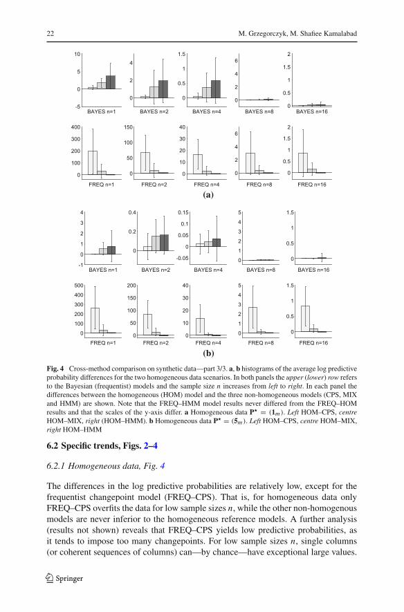
Fig. 4 Cross-method comparison on synthetic data—part 3/3. a, b histograms of the average log predictiveprobability differences for the two homogeneous data scenarios. In both panels the upper (lower) row refersto the Bayesian (frequentist) models and the sample size n increases from left to right. In each panel thedifferences between the homogeneous (HOM) model and the three non-homogeneous models (CPS, MIXand HMM) are shown. Note that the FREQ–HMM model results never differed from the FREQ–HOMresults and that the scales of the y-axis differ. a Homogeneous data P� = (1m ). Left HOM–CPS, centreHOM–MIX, right (HOM–HMM). b Homogeneous data P� = (5m ). Left HOM–CPS, centre HOM–MIX,right HOM–HMM
6.2 Specific trends, Figs. 2–4
6.2.1 Homogeneous data, Fig. 4
The differences in the log predictive probabilities are relatively low, except for thefrequentist changepoint model (FREQ–CPS). That is, for homogeneous data onlyFREQ–CPS overfits the data for low sample sizes n, while the other non-homogenousmodels are never inferior to the homogeneous reference models. A further analysis(results not shown) reveals that FREQ–CPS yields low predictive probabilities, asit tends to impose too many changepoints. For low sample sizes n, single columns(or coherent sequences of columns) can—by chance—have exceptional large values.
123
Comparative evaluation of Poisson counting models 23
AVERAGE OF FREQ AND BAYES-4000 -3000 -2000 -1000 0
DIF
FEE
RE
NC
E B
AY
ES
- FR
EQ
0
50
100
150
200 reference linechangepointsfree mixturehidden Markovhomogeneous
AVERAGE OF FREQ AND BAYES-6000 -5000 -4000 -3000 -2000 -1000 0
DIF
FER
EN
CE
BA
YE
S -
FRE
Q
0
50
100
150
200
250
AVERAGE OF FREQ AND BAYES
-7000 -6000 -5000 -4000 -3000 -2000 -1000 0
DIF
FER
EN
CE
BA
YE
S -
FRE
Q
-700
-600
-500
-400
-300
-200
-100
0
100
200
AVERAGE OF FREQ AND BAYES
-6000 -4000 -2000 0
DIF
FER
EN
CE
BA
YE
S -
FRE
Q
-1000
-800
-600
-400
-200
0
200
reference linechangepointsfree mixturehidden Markovhomogeneous
(a)
(b)
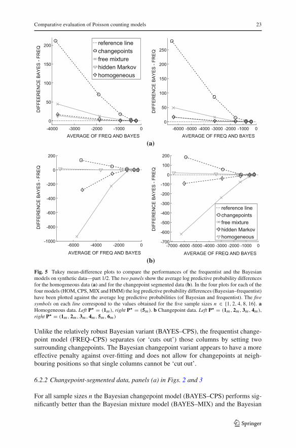
Fig. 5 Tukey mean-difference plots to compare the performances of the frequentist and the Bayesianmodels on synthetic data—part 1/2. The two panels show the average log predictive probability differencesfor the homogeneous data (a) and for the changepoint segmented data (b). In the four plots for each of thefour models (HOM, CPS,MIX and HMM) the log predictive probability differences (Bayesian–frequentist)have been plotted against the average log predictive probabilities (of Bayesian and frequentist). The fivesymbols on each line correspond to the values obtained for the five sample sizes n ∈ {1, 2, 4, 8, 16}. aHomogeneous data. Left P� = (1m ), right P� = (5m ). b Changepoint data. Left P� = (1m , 2m , 3m , 4m ),right P� = (1m , 2m , 3m , 4m , 5m , 6m )
Unlike the relatively robust Bayesian variant (BAYES–CPS), the frequentist change-point model (FREQ–CPS) separates (or ‘cuts out’) those columns by setting twosurrounding changepoints. The Bayesian changepoint variant appears to have a moreeffective penalty against over-fitting and does not allow for changepoints at neigh-bouring positions so that single columns cannot be ‘cut out’.
6.2.2 Changepoint-segmented data, panels (a) in Figs. 2 and 3
For all sample sizes n the Bayesian changepoint model (BAYES–CPS) performs sig-nificantly better than the Bayesian mixture model (BAYES–MIX) and the Bayesian
123

24 M. Grzegorczyk, M. Shafiee Kamalabad
AVERAGE OF FREQ AND BAYES-6000 -4000 -2000 0
DIF
FER
EN
CE
BA
YE
S -
FRE
Q
-1200
-1000
-800
-600
-400
-200
0
reference linechangepointsfree mixturehidden Markovhomogeneous
AVERAGE OF FREQ AND BAYES
-8000 -6000 -4000 -2000 0
DIF
FER
EN
CE
BA
YE
S -
FRE
Q
-1000
-800
-600
-400
-200
0
AVERAGE OF FREQ AND BAYES
-6000 -4000 -2000 0
DIF
FER
EN
CE
BA
YE
S -
FRE
Q
-1000
-800
-600
-400
-200
0
200
reference linechangepointsfree mixturehidden Markovhomogeneous
AVERAGE OF FREQ AND BAYES-6000 -4000 -2000 0
DIF
FER
EN
CE
BA
YE
S -
FRE
Q
-1000
-800
-600
-400
-200
0
200
(a)
(b)
Fig. 6 Tukey mean-difference plots to compare the performances of the frequentist and the Bayesianmodels on synthetic data—part 2/2. The two panels show the average log predictive probability differ-ences plotted against the average log predictive probabilities for the mixture data (a) and for the hiddenMarkov model data (b); for further details see caption of Fig. 5. aMixture data. Left P� = MIX(1m , 5m ),right P� = MIX(1m , 2m , 4m , 8m ). b Hidden Markov data. Left P� = (1m , 5m , 1m , 5m ), right P� =(1m , 5m , 1m , 5m , 1m , 5m ).
hidden Markov model (BAYES–HMM). The differences to the reference model(BAYES–CPS) show that BAYES–MIX performs consistently worse than BAYES–HMM. The reason becomes obvious from Fig. 8 in Sect. 7: BAYES–HMM approxi-mates the underlying allocation better than BAYES–MIX, as BAYES–HMM—unlikeBAYES–MIX—does not ignore the temporal order of the data points. For the frequen-tist models, the trend on changepoint-segmented data is slightly different: For smalln ≤ 2 there is no difference in the performance of the non-homogeneous models.Only for n ≥ 4 the changepoint model (FREQ–CPS) performs better than its com-petitors. Thereby the mixture model (FREQ–MIX) performs better than the hiddenMarkov model (FREQ–HMM) for n ≥ 4. Figure 9 in Sect. 7 suggests that this can be
123

Comparative evaluation of Poisson counting models 25
explained as follows: FREQ–MIX possesses fewer parameters than FREQ–HMM(seeTable 1) so that its BIC-penalty is lower (see Fig. 9). Consequently, FREQ–MIX canapproximate the underlying segmentation better than FREQ–HMM. For low n ≤ 2there is no difference between FREQ–CPS and the other models, as the frequentistchangepoint model (FREQ–CPS) tends to overfit the data, as discussed above (seehomogeneous data) and demonstrated in Sect. 7 (see Fig. 10).
6.2.3 Free-mixture data, panels (b) in Figs. 2 and 3
The Bayesian and the frequentist models show very similar trends. The changepointmodels (CPS) are substantially outperformed by the free mixture reference models(MIX),while the hiddenMarkovmodels (HMM)are competitive to themixturemodels(MIX). Only for small n ≤ 2 FREQ–HMM appears to be slightly inferior to FREQ–MIX. Figure 9 in Sect. 7 suggests that this is due to the higher BIC-penalty of theFREQ–HMMmodel. However, for the scenarioMIX(1m, 5m) and n = 1 the increasedBIC-penalty turns out to be advantageous for FREQ–HMM. Unlike FREQ–HMM,FREQ–MIX tends to overfit the data with n = 1 by re-allocating outliers (columnswith large values) to additional components.
6.2.4 Hidden-Markov data, panels (c) in Figs. 2 and 3
Among the Bayesian models, the mixture model (BAYES–MIX) is clearly outper-formed by the hidden Markov model (BAYES–HMM) for low sample sizes n ≤ 4.For larger sample sizes n ≥ 8 the differences decrease. The Bayesian changepointmodel (BAYES–CPS) is competitive to BAYES–HMM, as it approximates the under-lying dependency structure by additional changepoints; see Fig. 8 in Sect. 7.12 For thefrequentist models a complementary trend can be observed: The changepoint model(FREQ–CPS) is consistently inferior to the reference model (FREQ–HMM), whilethe mixture model (FREQ–MIX) is competitive for all n. Again FREQ–CPS tends tooverfit the data (by cutting out columns with large realisations by surrounding change-points), see Fig. 8 in Sect. 7. The disadvantage of FREQ–MIX, to ignore the temporalorder of the data points, appears to be compensated by its relatively low BIC-penalty(see Fig. 9 in Sect. 7).
6.3 Bayesian versus frequentist
The Tukey-mean-difference plots of the pairwise predictive probability differencesbetween the four Bayesian and the four frequentist models in Figs. 5 and 6 show thatboth paradigms yield nearly identical results for large sample sizes (n ≥ 8), whilesignificant differences can be observed for small sample sizes n. Most remarkablyare the following two trends: (i) Except for the mixture data [panel (a) in Fig. 6],
12 Note that the selected Poisson means (θ = 1 and θ = 5) yield components with very dissimilar values.This makes it easy for the changepoint model to distinguish them and to approximate the non-stationarityby setting an increased number of changepoints, e.g. 3 changepoints for (1m , 5m , 1m , 5m ).
123

26 M. Grzegorczyk, M. Shafiee Kamalabad
for low sample sizes n the Bayesian changepoint model (BAYES–CPS) is superiorto the frequentist changepoint model (FREQ–CPS). (ii) Except for the homogeneousdata [panel (a) in Fig. 5], the frequentist hidden Markov model (FREQ–HMM) andespecially the frequentist mixture model (FREQ–MIX) are superior to their Bayesiancounterparts (BAYES–HMM and BAYES–MIX). The reason for the superiority of theBayesian changepoint model (BAYES–CPS) is that the frequentist variant (FREQ–CPS) has a clear tendency towards over-fitting for uninformative data (for low n); seeFigs. 8 and 10 in Sect. 7 for more details. Unlike the Bayesian changepoint-modelinstantiation, FREQ–CPS infers only one single allocation vector (changepoint set)without any model-averaging. The low number of parameters of FREQ–CPS (seeTable 1) yields a relatively low BIC-penalty. Single columns of the data matrix, whichby chance have larger values than the other columns, can be ‘cut out’ so that the FREQ–CPS model is very susceptible to over-fitting. On the other hand, the superiority of thefrequentist mixture (FREQ–MIX) and the frequentist hidden Markov model (FREQ–HMM) over its Bayesian counterparts can be explained by the Multinomial-Dirichletprior on the allocation vector. Both Bayesian models (BAYES–MIX and BAYES–HMM)employMultinomial-Dirichlet priors for the allocation vectors,which can yieldvery strong prior penalties for non-homogeneous allocation vectors. As shown in Fig. 9in Sect. 7, BAYES–MIX is strongly penalized for all forms of non-homogeneity andBAYES–HMM is strongly penalized for mixture allocation vectors. This bottleneckof the Multinomial-Dirichlet prior for allocation vectors has already been analysedand discussed in Grzegorczyk et al. (2010) and renders the Bayesian model variantsinappropriate for small samples sizes n, i.e. for uninformative data, where the effectof the likelihood is small compared to the effect of the Multinomial-Dirichlet prior.
6.4 The New York City Taxi (NYCT) data
The results for the NYCT data are shown in Fig. 7. The top plots shows the averagelog predictive probabilities for the Bayesian models (left) and the frequentist models(right) for different sample sizes n. The lower panel provides Tukey mean-differenceplots to visualise the pairwise differences between the Bayesian and the frequen-tist models. The upper plots show that the homogeneous models (FREQ–HOM andBAYES–HOM) perform show the worst performance on the NYCT data. This is notunexpected, as Fig. 1 shows that the Taxi pick-up data are clearly non-stationary.Among the Bayesian models, the changepoint-model (BAYES–CPS) performs bestfor all sample sizes n, and asymptotically (i.e. as n increases) the non-homogeneousBayesian models perform equally well. Among the frequentist models the mixturemodel (FREQ–MIX) shows the best performance. For n = 1 FREQ–MIX and FREQ–HMM perform approximately equally well, while FREQ–CPS performs significantlyworse. For n = 2 the FREQ–MIX model performs better than both competitors. Andfor larger n (n ≥ 4) FREQ–MIX and FREQ–CPS perform equally well, while FREQ–HMMperforms slightly worse. The Tukeymean-difference plot in the bottom of Fig. 7shows that the Bayesian and frequentist models asymptotically perform equally well.For the lower samples sizes n the trends are consistent with the earlier observations forthe synthetic data. The Bayesian changepoint model (BAYES–CPS) is superior to its
123

Comparative evaluation of Poisson counting models 27
samples n per time point1 2 4 8 16
AV
ER
AG
E P
RE
DIC
TTIV
E P
RO
BA
BIL
ITY
-7800
-7600
-7400
-7200
-7000
-6800
-6600
-6400
-6200BAYESIAN APPROACHES
homogeneouschangepointsfree mixturehidden Markov
samples n per time point1 2 4 8 16
AV
ER
AG
E P
RE
DIC
TIV
E P
RO
BA
BIL
ITY
-7800
-7600
-7400
-7200
-7000
-6800
-6600
-6400
-6200FREQUENTIST APPROACHES
AVERAGE OF FREQ AND BAYES
-6900 -6800 -6700 -6600 -6500 -6400 -6300DIF
FER
EN
CE
BA
YE
S -
FRE
Q
-800
-600
-400
-200
0
200
400BAYESIAN vs. FREQUENTIST
reference linechangepointsfree mixturehidden Markov
Fig. 7 Results for the New York City Taxi data. In the upper plots the average log predictive probabilities(averaged across 35 data sets; i.e. 5 randomly sampled data instantiations per weekday) of the Bayesianmodels (upper left) and the frequentist models (upper right) have been plotted against the number of samplesn per time point t . In the lower plot for each of the three non-homogeneous models (CPS, MIX and HMM)the average log predictive probability differences (BAYES–FREQ) have been plotted against the averagelog predictive probability of FREQ and BAYES. The five symbols on each line correspond to the valuesobtained for the sample sizes n ∈ {1, 2, 4, 8, 16}. In the lower plot the Bayesian (frequentist) model issuperior when the curve/symbol is above (below) the reference line
frequentist counterpart (FREQ–CPS), while the opposite trend can be observed for themixture and the hidden Markov model. The p values of two-sided one-sample t testsfor the predictive probability differences between the best Bayesian model (BAYES–CPS) and the best frequentist model (FREQ–CPS) are computed to determine whetherthe performances differ significantly for any n. Given the relatively small t test samplesize of nd = 7 weekdays,13 the five p values (for n = 1, 2, 4, 8, 16) are higher thanthe standard level α = 0.05, indicating that the best Bayesian and the best frequentistmodel are performing approximately equally well on the NYCT data.14
13 That is one (average) predictive probability difference per weekday; the differences for the 5 datareplicates per weekday are averaged, as they are very similar to each other.14 p values: p = 0.30 (n = 1), 0.53 (n = 2), p = 0.96 (n = 4), p = 0.45 (n = 8), and p = 0.72 (n = 16).
123

28 M. Grzegorczyk, M. Shafiee Kamalabad
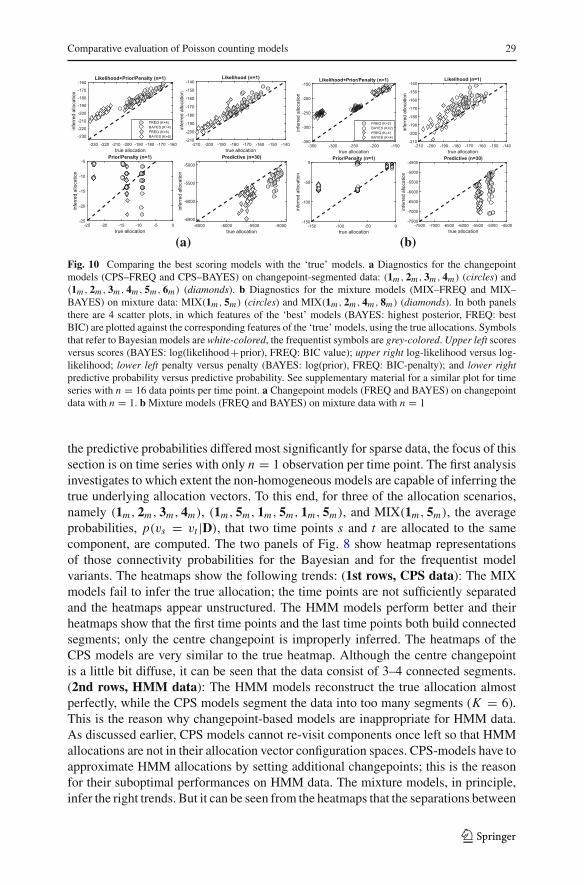
(a) (b)
Fig. 8 Heatmap representations of the inferred connectivity structures for the non-homogeneous mod-els. a Refers to the Bayesian models, b to the frequentist models. Both panels are arranged as 3-by-4matrices with rows corresponding to the true allocation vectors: CPS: (1m , 2m , 3m , 4m ) (top), HMM:(1m , 5m , 1m , 5m , 1m , 5m ) (centre), and MIX: MIX(1m , 5m ) (bottom). The first columns show the trueconnectivity structures, and rows 2–4 correspond to the three non-homogeneous models: CPS, HMM, andMIX. The heatmaps give the inferred probabilities p(vs = vt |D) of two points s and t belonging to thesame component. The probabilities are represented by a grey shading, where white corresponds to 1, andblack corresponds to 0. The axes refer to the T = 96 time points. All connectivity probabilities p(vs = vt )
are averaged over 25 data instantiations with n = 1 observation per time point. The time points of the MIXdata in the last rows have been ordered w.r.t. the two mixture components. a Heatmaps of Bayesian modelvariants. b Heatmaps of frequentist model variants
V1 V2FREQ
PEN
ALT
Y
-200
-100
0CPS data
-200
-100
0HMM data
CPS modelMIX modelHMM model
-200
-100
0MIX data
BA
YES
PRIO
R
-200
-100
0
-200
-100
0V1 V2 V1 V2
V1 V2 V1 V2 V1 V2-200
-100
0
Fig. 9 Comparison of penalty terms for the non-homogeneous models. The plot is arranged as a 2-by-3matrix, and the rows refer to the frequentist (top) and the Bayesian (bottom) models. The columns refer tothree different allocation scenarios (CPS data, HMMdata, andMIX data) and for each scenario two variants(V1 and V2) are distinguished. The segmentation schemes correspond to those used in the comparativeevaluation study in Sect. 6, see Table 2 in the supplementary material for an overview. The bars give thepenalties (BIC or prior probability) of the three models (CPS, MIX and HMM) for the true underlyingallocation. As the CPS models cannot infer the true allocation of mixture data, the bars are not shown. Forthe CPS models it is assumed that they approximate HMM data by additional changepoints, e.g. (HMM,V1): (1m , 5m , 1m , 5m ) is approximated by setting 3 changepoints
7 Further model diagnostics
This section provides additional diagnostic plots for the synthetic data, analysed inSect. 6. The goal is to shed more light onto the relative merits and shortcomings of themodels under comparison and to derive some conclusions of general validity. Since
123
Comparative evaluation of Poisson counting models 29
true allocation-230 -220 -210 -200 -190 -180 -170 -160
infe
rred
allo
catio
n
-230
-220
-210
-200
-190
-180
-170
-160Likelihood+Prior/Penalty (n=1)
FREQ (K=4)BAYES (K=4)FREQ (K=6)BAYES (K=6)
true allocation-210 -200 -190 -180 -170 -160 -150 -140
infe
rred
allo
catio
n
-210
-200
-190
-180
-170
-160
-150
-140Likelihood (n=1)
true allocation-25 -20 -15 -10 -5 0
infe
rred
allo
catio
n
-25
-20
-15
-10
-5Prior/Penalty (n=1)
true allocation-6500 -6000 -5500 -5000
infe
rred
allo
catio
n
-6500
-6000
-5500
-5000
Predictive (n=30)true allocation
-350 -300 -250 -200 -150
infe
rred
allo
catio
n
-350
-300
-250
-200
-150Likelihood+Prior/Penalty (n=1)
FREQ (K=2)BAYES (K=2)FREQ (K=4)BAYES (K=4)
true allocation-210 -200 -190 -180 -170 -160 -150 -140
infe
rred
allo
catio
n
-210
-200
-190
-180
-170
-160
-150
-140Likelihood (n=1)
true allocation-150 -100 -50 0
infe
rred
allo
catio
n
-150
-100
-50
0Prior/Penalty (n=1)
true allocation-7500 -7000 -6500 -6000 -5500 -5000 -4500
infe
rred
allo
catio
n
-7500
-7000
-6500
-6000
-5500
-5000
-4500Predictive (n=30)
(a) (b)
Fig. 10 Comparing the best scoring models with the ‘true’ models. a Diagnostics for the changepointmodels (CPS–FREQ and CPS–BAYES) on changepoint-segmented data: (1m , 2m , 3m , 4m ) (circles) and(1m , 2m , 3m , 4m , 5m , 6m ) (diamonds). b Diagnostics for the mixture models (MIX–FREQ and MIX–BAYES) on mixture data: MIX(1m , 5m ) (circles) and MIX(1m , 2m , 4m , 8m ) (diamonds). In both panelsthere are 4 scatter plots, in which features of the ‘best’ models (BAYES: highest posterior, FREQ: bestBIC) are plotted against the corresponding features of the ‘true’ models, using the true allocations. Symbolsthat refer to Bayesian models are white-colored, the frequentist symbols are grey-colored. Upper left scoresversus scores (BAYES: log(likelihood+prior), FREQ: BIC value); upper right log-likelihood versus log-likelihood; lower left penalty versus penalty (BAYES: log(prior), FREQ: BIC-penalty); and lower rightpredictive probability versus predictive probability. See supplementary material for a similar plot for timeseries with n = 16 data points per time point. a Changepoint models (FREQ and BAYES) on changepointdata with n = 1. b Mixture models (FREQ and BAYES) on mixture data with n = 1
the predictive probabilities differed most significantly for sparse data, the focus of thissection is on time series with only n = 1 observation per time point. The first analysisinvestigates to which extent the non-homogeneous models are capable of inferring thetrue underlying allocation vectors. To this end, for three of the allocation scenarios,namely (1m, 2m, 3m, 4m), (1m, 5m, 1m, 5m, 1m, 5m), and MIX(1m, 5m), the averageprobabilities, p(vs = vt |D), that two time points s and t are allocated to the samecomponent, are computed. The two panels of Fig. 8 show heatmap representationsof those connectivity probabilities for the Bayesian and for the frequentist modelvariants. The heatmaps show the following trends: (1st rows, CPS data): The MIXmodels fail to infer the true allocation; the time points are not sufficiently separatedand the heatmaps appear unstructured. The HMM models perform better and theirheatmaps show that the first time points and the last time points both build connectedsegments; only the centre changepoint is improperly inferred. The heatmaps of theCPS models are very similar to the true heatmap. Although the centre changepointis a little bit diffuse, it can be seen that the data consist of 3–4 connected segments.(2nd rows, HMM data): The HMM models reconstruct the true allocation almostperfectly, while the CPS models segment the data into too many segments (K = 6).This is the reason why changepoint-based models are inappropriate for HMM data.As discussed earlier, CPS models cannot re-visit components once left so that HMMallocations are not in their allocation vector configuration spaces. CPS-models have toapproximate HMM allocations by setting additional changepoints; this is the reasonfor their suboptimal performances on HMM data. The mixture models, in principle,infer the right trends. But it can be seen from the heatmaps that the separations between
123

30 M. Grzegorczyk, M. Shafiee Kamalabad
the components are weaker than those of the HMM models. (3rd rows, MIX data):The CPS models fail to infer the segmentation of the mixture data. The HMM andthe MIX models perform approximately equally well and correctly divide the timepoints into K = 2 components, though the inferred separations appear to be slightlytoo weak. (BAYESIAN vs. FREQ): The heatmaps of the Bayesian and the frequentistmodel variants are very similar, except for the heatmaps of the changepoint-models onmixture data (see bottom rows, 2nd columns in Fig. 8). While CPS–BAYES does notseparate the time points, the frequentist counterpart (CPS–FREQ) shows the oppositebehaviour: CPS–FREQ separates the time points into (too) many short segments.
Overall, the findings are in agreement with the results from Sect. 6: The heatmapsin Fig. 8 confirm that the HMM models can properly infer HMM data and mixturedata while their performances on changepoint-segmented data are suboptimal (thechangepoints are not properly inferred). The CPS models and the MIX models com-pletely fail for certain allocation scenarios: The CPS model cannot deal with mixturedata and can only approximate the segmentation of HMM data by setting too manychangepoints. The mixture models, which do not exploit the temporal order of thedata points, are inappropriate for changepoint-segmented data. Another finding is thedifference between the two changepoint models: CPS–BAYES and CPS–FREQ. Formixture data CPS–BAYES infers ‘undercomplex’ allocations with too few change-points (mostly K = 1), while CPS–FREQ infers ‘overcomplex’ allocations with toomany changepoints (even the maximum of K = 10 changepoints is reached). Thelatter finding suggests that the frequentist changepoint model has a tendency towardsoverfitting the data by setting too many changepoints.
A comparison of the penalty terms for the true allocations is given in Fig. 9. Thetop row of Fig. 9 shows the BIC-penalties of the frequentist models, the bottom rowshows the Bayesian (log) prior probability penalties. (CPS data andHMMdata) Thepenalties of the frequentist and the Bayesian models are comparable except for theMIX model. For both types of data the penalties of the Bayesian mixture model aresubstantially higher than the penalties of its frequentist counterpart. (MIX data) TheCPS model cannot infer the true mixture allocations. The Bayesian HMM model andthe Bayesian MIX model are penalized significantly stronger than their frequentistcounterparts. (MIX–BAYES vs. HMM–BAYES) The bottom row of Fig. 9 showsthat the penalties of HMM–BAYES andMIX–BAYES are nearly identical for mixturedata, while MIX–BAYES has substantially higher penalties for CPS data and MIXdata. That is, the Bayesian mixture model (MIX–BAYES) is ‘over-penalized’ for non-mixture data.
The last diagnostic compares the performances of the Bayesian and the frequentistmodels with respect to over-fitting issues. To this end, certain ‘features’ of the ‘best’inferred models (FREQ-models minimising the BIC score; BAYES-models with thehighest posterior score) are compared with the corresponding ‘features’ of the truemodels, i.e. models which are based on the true allocation vectors. The ‘features’ are:(i) the scores, (ii) the (marginal) likelihood values, (iii) the prior penalty terms, and(iv) the predictive probabilities for new data. Figure 10 gives scatter plots in whichthe features of the best inferred models are plotted against the features of the truemodels. The scatter plots can be interpreted as follows: Symbols are above (below) thediagonal when the feature of the best inferred model is higher (lower) than the feature
123

Comparative evaluation of Poisson counting models 31
of the true model. (Figure 10a, changepoint-divided data): The best inferred modelsyield higher scores and higher likelihoods than the true models. That is, both modelsvariants (BAYES and FREQ) fit the data better than the true models. But the scatterplot of the penalty terms show that the Bayesian CPSmodel consistently infers ‘under-penalized’ models (i.e. models with too few changepoints) while the frequentist CPSmodel also infers ‘over-penalized’ models (i.e. models with too many changepoints).The scatter plot of the predictive probabilities shows the implication. The inferredmodels are inferior to the true models (all symbols are below the diagonal), but thepredictive probabilities of the ‘under-complex’ CPS–BAYES model are better thanthose of the ‘over-complex’ CPS–FREQ model. Thereby the most ‘over-complex’CPS–FREQ models yield the lowest predictive probabilities. This clearly shows thatthe frequentist changepoint model is more susceptible to over-fitting than its Bayesiancounterpart. (Figure 10b, mixture data): The upper panels show that MIX–FREQagain consistently overfits the data, while the MIX–BAYES model sometimes yieldslower likelihoods than the true model (see diamond symbols in the upper right panel).The scatter plot of the penalty term shows that MIX–BAYES infers ‘undercomplex’models (with too few mixture components) for scenario (V2, mixture with K = 4components) and sometimes for scenario (V1, mixture with K = 2 components). Thissuggests that MIX–BAYES overpenalizes the complexity of the allocation vectors, sothat ‘undercomplex’ models are inferred. This explains why MIX–FREQ is superiorto the over-penalized (and thus ‘undercomplex’) MIX–BAYESmodel (see scatter plotof the predictive probabilities). Figure 1 in the supplementary material shows the samediagnostics for time series with n = 16 data points per time point. The results showthat those issues of under- and over-penalisation diminish/disappear as the data getmore informative.
Summary
The additional diagnostics, shown in Figs. 8, 9 and 10, confirm four of the empiricalfindings from Sect. 6.
1. In Sect. 6 the CPS-models showed suboptimal performances for HMM and MIXdata. Figure 8 shows that CPSmodels are inferior toHMMmodels for both types ofdata because the true allocations are not part of their allocation vector configurationspaces. Only for changepoint segmented data, where the HMM models do notproperly infer the true allocation, theCPSmodels are superior to theHMMmodels.
2. In Sect. 6 the MIX-models showed suboptimal performances for CPS and HMMdata. Figure 8 shows that the MIX models cannot properly infer CPS and HMMallocations, while the HMMmodels show moderate performances for all types ofdata.
3. In Sect. 6 the Bayesian mixture model (MIX–BAYES) was found to be inferiorto its frequentist counterpart (MIX–FREQ). As seen from Figs. 9 and 10, theBayesian mixture variant is over-penalised. This renders the frequentist HMMmodel preferable to the Bayesian mixture model.
4. In Sect. 6 itwas also found that theBayesianCPSmodel is superior to its frequentistcounterpart (CPS–FREQ). As seen from Fig. 10a, the frequentist changepoint
123

32 M. Grzegorczyk, M. Shafiee Kamalabad
model tends to overfit the data. This renders the Bayesian changepoint modelpreferable to the frequentist CPS model.
8 Conclusions
In this paper the results of a comparative evaluation study on eight (non-)homogeneousmodels for (Poisson) count data were presented. The study was performed on varioussynthetic data sets and on taxi pick-up counts, extracted from the recently publishedNewYork City Taxi (NYCT) database, described in Sect. 4. For the study the standardhomogeneous Poisson model (HOM) and three non-homogeneous Poisson models,namely a changepoint model (CPS), a free mixture model (MIX) and a hiddenMarkovmodel (HMM), were implemented following the frequentist paradigm (FREQ) andthe Bayesian paradigm (BAYES); see Tables 1 and 2 in Sect. 2 for an overview. Theempirical findings from Sects. 6 and 7 suggest the following conclusions:
Asymptotically, i.e. for sufficiently informative data (here: quantified in terms ofthe sample size n per time point t), there is no difference between the paradigms.The Bayesian and the frequentist models perform equally well. For less informativedata (here: for small n) there are significant differences, as described in more detailbelow. While the homogeneous model variants (FREQ–HOM and BAYES–HOM)cannot deal with non-homogeneity, the non-homogeneous models, except for the fre-quentist changepoint model (FREQ–CPS), do not overfit homogeneous data. Thus, itcan be recommended applying non-homogeneous approaches, even if the data mightbe homogeneous. Moreover, if the data is informative enough, in both frameworks(Bayesian and frequentist) all three non-homogeneous models can approximate allkinds of non-homogeneity, unless there is a clear mismatch between the model andthe underlying data. E.g. in Sects. 6 and 7 it was found that the changepoint models(FREQ–CPS and BAYES–CPS) perform badly for mixture data. The hidden Markovmodels (FREQ–HMM and BAYES–HMM) appear to be superior to the mixture mod-els (FREQ–MIX and BAYES–MIX), since they are competitive on free-mixture data,and superior on hidden Markov and changepoint-segmented data.15 In a pairwisecomparison of the four Bayesian and the four frequentist models it was found forless informative data (here: small n) that the Bayesian changepoint model (BAYES–CPS) is superior to its frequentist counterpart (FREQ–CPS), while the opposite trendcould be observed for the mixture model and the hidden Markov model. The superi-ority of the Bayesian changepoint model (BAYES–CPS) over the frequentist variant(FREQ–CPS) is due to the fact the the frequentist model variant is very susceptibleto over-fitting (see Fig. 10a in Sect. 7). The inferiority of the Bayesian free mixturemodel (BAYES–MIX) and the Bayesian hidden Markov (BAYES–HMM) model totheir frequentist counterparts is caused by the allocation vector priors. Both Bayesianmodels employ the Multinomial-Dirichlet prior, which is known to impose a verystrong penalty on non-homogeneous allocations (see Fig. 9 in Sect. 7), rendering theBayesian variants inappropriate for less informative data sets (here: for small samples
15 Though still worse than the changepoint models (FREQ–CPS and BAYES–CPS), which can be seen asreference models for changepoint-segmented data.
123
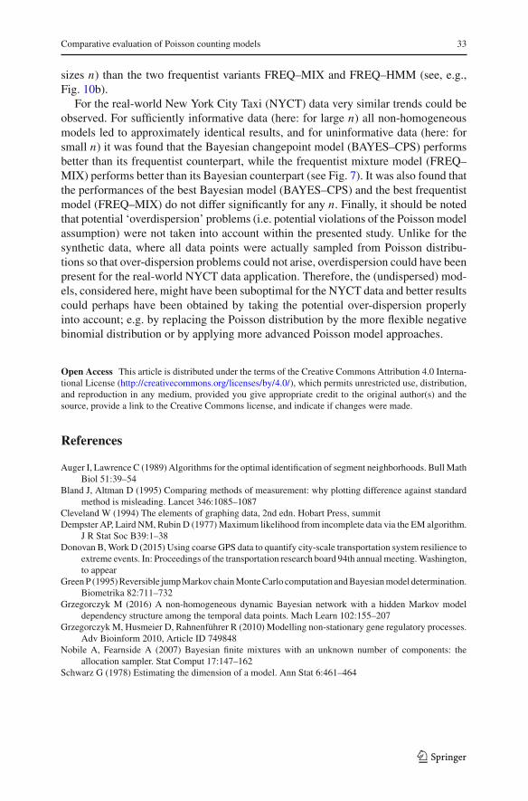
Comparative evaluation of Poisson counting models 33
sizes n) than the two frequentist variants FREQ–MIX and FREQ–HMM (see, e.g.,Fig. 10b).
For the real-world New York City Taxi (NYCT) data very similar trends could beobserved. For sufficiently informative data (here: for large n) all non-homogeneousmodels led to approximately identical results, and for uninformative data (here: forsmall n) it was found that the Bayesian changepoint model (BAYES–CPS) performsbetter than its frequentist counterpart, while the frequentist mixture model (FREQ–MIX) performs better than its Bayesian counterpart (see Fig. 7). It was also found thatthe performances of the best Bayesian model (BAYES–CPS) and the best frequentistmodel (FREQ–MIX) do not differ significantly for any n. Finally, it should be notedthat potential ‘overdispersion’ problems (i.e. potential violations of the Poisson modelassumption) were not taken into account within the presented study. Unlike for thesynthetic data, where all data points were actually sampled from Poisson distribu-tions so that over-dispersion problems could not arise, overdispersion could have beenpresent for the real-world NYCT data application. Therefore, the (undispersed) mod-els, considered here, might have been suboptimal for the NYCT data and better resultscould perhaps have been obtained by taking the potential over-dispersion properlyinto account; e.g. by replacing the Poisson distribution by the more flexible negativebinomial distribution or by applying more advanced Poisson model approaches.
Open Access This article is distributed under the terms of the Creative Commons Attribution 4.0 Interna-tional License (http://creativecommons.org/licenses/by/4.0/), which permits unrestricted use, distribution,and reproduction in any medium, provided you give appropriate credit to the original author(s) and thesource, provide a link to the Creative Commons license, and indicate if changes were made.
References
Auger I, Lawrence C (1989) Algorithms for the optimal identification of segment neighborhoods. BullMathBiol 51:39–54
Bland J, Altman D (1995) Comparing methods of measurement: why plotting difference against standardmethod is misleading. Lancet 346:1085–1087
Cleveland W (1994) The elements of graphing data, 2nd edn. Hobart Press, summitDempster AP, Laird NM, Rubin D (1977)Maximum likelihood from incomplete data via the EM algorithm.
J R Stat Soc B39:1–38Donovan B,Work D (2015) Using coarse GPS data to quantify city-scale transportation system resilience to
extreme events. In: Proceedings of the transportation research board 94th annual meeting.Washington,to appear
GreenP (1995)Reversible jumpMarkov chainMonteCarlo computation andBayesianmodel determination.Biometrika 82:711–732
Grzegorczyk M (2016) A non-homogeneous dynamic Bayesian network with a hidden Markov modeldependency structure among the temporal data points. Mach Learn 102:155–207
Grzegorczyk M, Husmeier D, Rahnenführer R (2010) Modelling non-stationary gene regulatory processes.Adv Bioinform 2010, Article ID 749848
Nobile A, Fearnside A (2007) Bayesian finite mixtures with an unknown number of components: theallocation sampler. Stat Comput 17:147–162
Schwarz G (1978) Estimating the dimension of a model. Ann Stat 6:461–464
123