COMPARATIVE STUDIES OF DIFFERENT SYSTEM MODELS FOR

ITERATIVE CT IMAGE RECONSTRUCTION

BY

CHUANG MIAO

A Thesis Submitted to the Graduate Faculty of

WAKE FOREST UNIVERSITY GRADUATE SCHOOL OF ARTS AND

SCIENCES

in Partial Fulfillment of the Requirements

for the Degree of

MASTER OF SCIENCE

Biomedical Engineering

MAY 2013

Winston-Salem, North Carolina

Approved by:

Hengyong Yu, Ph.D., Advisor

Ge Wang, Ph.D., Co-advisor, Chair

Guohua Cao, Ph.D.

ii

ACKNOWLEDGEMENTS

I would like to thank my advisor, Dr. Hengyong Yu, who first introduced me to the

wonderful world of CT image reconstruction. He devoted a great deal of time to

instruct me throughout the years. His inspiration, constant support and valuable

advice encouraged me to conquer the hardship both in research and life. I would

also like to thank my co-advisor, Dr. Ge Wang, whose valuable advices gave me

many inspirations. I learned a lot from his great vision and innovative thinking. I

would also like to thank all the lab members, such as Dr. Baodong Liu. Your

helpful discussions have been greatly appreciated. Finally, I would like to thank

my parents, sisters and brothers-in-law for their continued support. You are my

eternal source of driving force.

iii

TABLE OF CONTENTS

LIST OF TABLES .................................................................................................vi

LIST OF FIGURES .............................................................................................. vii

ABSTRACT ........................................................................................................ xiii

1. Introduction ....................................................................................................... 1

1.1 X-ray Computed Tomography ..................................................................... 1

1.2 Current CT Development ............................................................................ 1

1.2.1 First Generation CT Scanners .............................................................. 2

1.2.2 Second Generation CT Scanners ......................................................... 2

1.2.3 Third Generation CT Scanners ............................................................. 2

1.2.4 Fourth Generation CT Scanners .......................................................... 3

1.2.5 Fifth Generation CT Scanners .............................................................. 5

1.3 CT data measurement ................................................................................ 5

1.4 CT Image Display ....................................................................................... 9

1.5 Thesis Organization .................................................................................. 11

2. System Models ............................................................................................... 14

2.1 Representation as a Linear System .......................................................... 14

2.2 System Models ......................................................................................... 19

2.2.1 Pixel-driven Model .............................................................................. 19

iv

2.2.2 Ray-driven Model ............................................................................... 20

2.2.3 Area Integral Model ............................................................................ 20

2.2.4 Distance-driven Model ........................................................................ 21

2.2.5 Improved Distance-driven Model ........................................................ 23

2.3 Comparative Analysis of Different Models ................................................ 25

2.3.1 Pixel-driven Model .............................................................................. 26

2.3.2 Ray-driven Model ............................................................................... 27

2.3.3 Area Integral Model ............................................................................ 29

2.3.4 Distance-driven Model ........................................................................ 32

2.3.5 Improved Distance-driven Model ........................................................ 34

2.4 Experimental Analysis ............................................................................... 35

2.4.1 Projection of a Uniform Disk ............................................................... 38

2.4.2 Backprojection of a Uniform Projection ............................................... 39

2.4.3 Pixel Support ...................................................................................... 48

3. Iterative Image Reconstruction Algorithms ..................................................... 64

3.1 Overview ................................................................................................... 64

3.2 ART ........................................................................................................... 66

3.3 SART ........................................................................................................ 67

3.4 OS-SART .................................................................................................. 67

4. Experiments and Results ................................................................................ 69

v

4.1 Algorithm Workflow ................................................................................... 69

4.2 Physical Phantom Experiment .................................................................. 70

4.2.1 Computational Cost ............................................................................ 71

4.2.2 Image Noise ....................................................................................... 73

4.2.3 Spatial Resolution .............................................................................. 75

4.2.4 Structural SIMilarity (SSIM) ................................................................ 82

4.3 Discussion and Conclusion ....................................................................... 83

5. Conclusions and Future Work ........................................................................ 88

References ......................................................................................................... 90

Appendix A ......................................................................................................... 96

A.1 Distance-driven Kernel ............................................................................. 96

Curriculum Vitae ................................................................................................. 98

vi

LIST OF TABLES

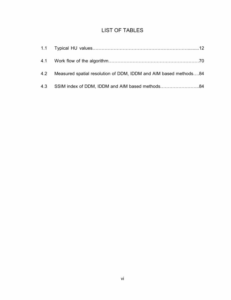
1.1 Typical HU values……………………………………………………….........12

4.1 Work flow of the algorithm……………………………………………………70

4.2 Measured spatial resolution of DDM, IDDM and AIM based methods….84

4.3 SSIM index of DDM, IDDM and AIM based methods……………………..84

vii

LIST OF FIGURES

1.1 Different generations of CT scanners…………….…….............................4

1.2 Fifth generation CT scanner…………….…….............................5

1.3 The attenuation process of an x-ray beam passing through an object with

(a) single layer; (b) multiple layers and (c) an arbitrary object….8

1.4 Gray level mapping with specific window level and window..................11

1.5 Same image with different display window level and window width…….12

2.1 Area integral model assuming a fan beam geometry………………..……21

2.2 Distance-driven model assuming a fan beam geometry…………..…23

2.3 Improved distance-driven model assuming a fan beam geometry….24

2.4 Pixel-driven model with one row image and multiple detector elements

assuming a 2D parallel-beam geometry………………………………28

2.5 Ray-driven model with one row image and one detector element

assuming a 2D parallel-beam geometry…………….…………………...…31

2.6 Area integral model with one row image and one detector element

assuming a 2D parallel-beam geometry………………………………...…33

2.7 Distance-driven model with one row image and one detector element

assuming a 2D parallel-beam geometry…………………………………...36

2.8 Improved distance-diven model with one row image and one detector

element assuming a 2D parallel-beam geometry……………………...37

viii

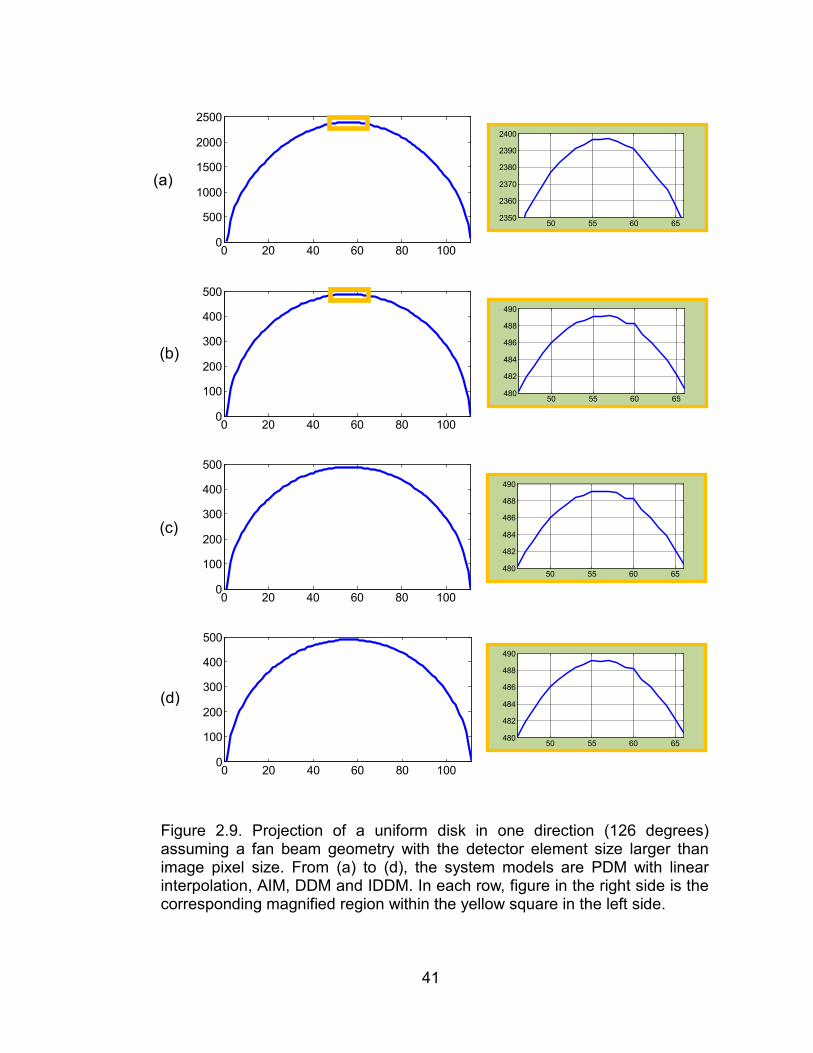
2.9 Projection of a uniform disk in one direction (126 degrees) assuming

a fan beam geometry with the detector element size larger than image

pixel size……………………………………………………………………….41

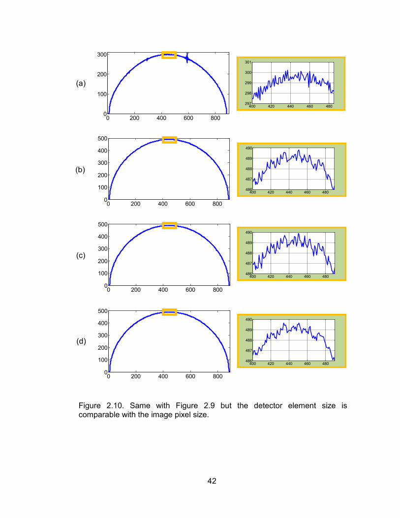
2.10 Same with Figure 2.9 but the detector element size is comparable

with the image pixel size…………………………………………………….42

2.11 Same with Figure 2.9 but the detector element size is smaller than

the image pixel size…………………………………………………………..43

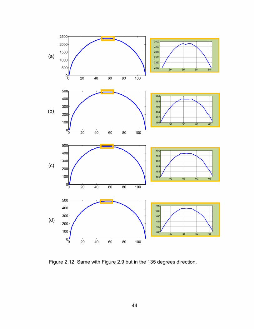
2.12 Same with Figure 2.9 but in the 135 degrees direction………………....44

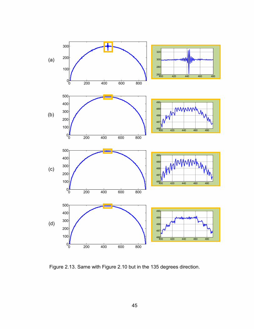
2.13 Same with Figure 2.10 but in the 135 degrees direction……………….…45

2.14 Same with Figure 2.11 but in the 135 degrees direction……………….…46

2.15 Backprojection of a uniform projection data in 126 degrees direction

assuming a fan beam geometry……………………………………………...50

2.16 Contour plots of the last three rows in Figure2.15………………………...50

2.17 Same with Figure 2.15 but in the 135 degrees direction………………….52

2.18 Contour plots of the last three rows in Figure2.17…………………...……52

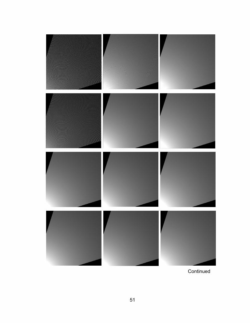
2.19 Pixel supports with image size 512 × 512 assuming a fan beam

geometry…………………...…………………………………………………...56

2.20 Contour plots of the last three rows in Figure2.19………………………...57

2.21 The line profiles of the 256th row in the image support…………………..59

2.22 Same with Figure 2.21 but for the second column of Figure 2.19, which

the detector element size is comparable with the image pixel size…..…61

ix

2.23 Same with Figure 2.21 but for the third column of Figure 2.19, which

the detector element size is smaller than the image pixel size…………63

4.1 The full view of the phantom…………………………………………………72

4.2 The computational cost of AIM and DDM and IDDM based methods in

one iteration for 512 × 512image sizes with different number of detector

cells in projection data………………………………………………………..72

4.3 The image noise (HU) versus the iteration numbers using four sets of

projections with different detector cell numbers………………...…………76

4.4 Reconstructed images from the projections with 888 detector cells…….77

4.5 Same as Figure 4.4 but reconstructed from the projections with 444

detector cells…………………………………………………………………..78

4.6 Same as Figure 4.4 but reconstructed from the projections with 222

detector cells…………………………………………………………………..79

4.7 Same as Figure 4.4 but reconstructed from the projections with 111

detector cells……………………………………………………………………80

4.8 The measured spatial resolution (mm) versus the iteration number for

four sets of projections with different detector cell numbers…………..85

4.9 Magnifications of the square region indicated in Figure 4.1. From top to

bottom, the detector cell numbers are 888, 444, 222 and 111,

respectively…………………………………………………………………….86

4.10 Same with Figure 4.9 but from 17 iterations…………………………87

x

A.1 Distance-driven kernel………………………………………………………..97

xi

LIST OF ABBREVIATION

AIM Area Integral Model

ART Algebraic Reconstruction Technique

CT Computed Tomography

EBCT Electron Beam Computed Tomography

FOV Field of View

FWHMs Full-width-of-half-maximums

HU Hounsfield Unit

IDDM Improved Distance-driven Model

IR Iterative Reconstruction

ML-EM Maximum Likelihood Expectation-maximization

MRI Magnetic Resonance Imaging

OS-SART Ordered Subset Simultaneous Algebraic

Reconstruction Technique

PDM Pixel-driven Model

PET Positron Emission Tomography

RDM Ray-driven Model

SART Simultaneous Algebraic Reconstruction Technique

SPECT Single Photon Emission Computed Tomography

xii

SSIM Structural SIMilarity

STP Standard Pressure and Temperature

xiii

ABSTRACT

In this thesis, we propose an improved distance-driven model (IDDM) whose

computational cost is as low as the distance-driven model (DDM) and the

accuracy is comparable with the area integral model (AIM). The performance of

different system models, such as pixel-driven model (PDM), ray-driven model

(RDM), AIM, DDM and IDDM, are compared in the content of iterative CT image

reconstruction algorithms. One of the key factors that limit the clinical application

of an iterative reconstruction algorithm is the high computational cost which

mainly depends on the system model. This thesis can serve as the basis for the

acceleration study and will have a direct impact on development of fast and

accurate iterative CT image reconstruction algorithms.

1

1. Introduction

1.1 X-ray Computed Tomography

The first commercial x-ray Computed Tomography (CT) prototype was built in

1972 by Godfrey Hounsfield, for which Hounsfield shared the Nobel Prize in 1979

with Cormack, who had independently developed the math foundation at Tufts

University in 1963. CT generates a 2D or 3D cross-sectional image of a scanning

object, such as human body, from projection data obtained from different

directions. This process is the so-called image reconstruction. Several other

imaging modalities exist such as Positron Emission Tomography (PET) [2-5].

Single Photon Emission Computed Tomography (SPECT) [6-8] and Magnetic

Resonance Imaging (MRI) [9-11]. Unlike CT, in PET and SPECT, the radioactive

material is the radiation source which is located inside the body. MRI used a

strong magnetic field to generate the internal structures of the body. CT is

currently the most widely used imaging modality because CT is fast, easy to use,

high resolution and relatively cheap than MRI or PET.

1.2 Current CT Development

Since the first commercial CT scanner was developed by Hounsfield in 1972, the

technology of CT scanners has been tremendous improved. The driven force

behind the scene is to achieve a better temporal resolution, a higher spatial

resolution and a faster image reconstruction. The development of CT scanners

can be distinctively marked by the beam geometry and the scanning trajectory.

2

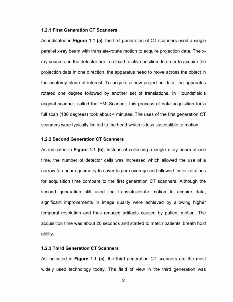
1.2.1 First Generation CT Scanners

As indicated in Figure 1.1 (a), the first generation of CT scanners used a single

parallel x-ray beam with translate-rotate motion to acquire projection data. The x-

ray source and the detector are in a fixed relative position. In order to acquire the

projection data in one direction, the apparatus need to move across the object in

the anatomy plane of interest. To acquire a new projection data, the apparatus

rotated one degree followed by another set of translations. In Houndsfield’s

original scanner, called the EMI-Scanner, this process of data acquisition for a

full scan (180 degrees) took about 4 minutes. The uses of the first generation CT

scanners were typically limited to the head which is less susceptible to motion.

1.2.2 Second Generation CT Scanners

As indicated in Figure 1.1 (b), Instead of collecting a single x-ray beam at one

time, the number of detector cells was increased which allowed the use of a

narrow fan beam geometry to cover larger coverage and allowed faster rotations

for acquisition time compare to the first generation CT scanners. Although the

second generation still used the translate-rotate motion to acquire data,

significant improvements in image quality were achieved by allowing higher

temporal resolution and thus reduced artifacts caused by patient motion. The

acquisition time was about 20 seconds and started to match patients’ breath hold

ability.

1.2.3 Third Generation CT Scanners

As indicated in Figure 1.1 (c), the third generation CT scanners are the most

widely used technology today. The field of view in the third generation was

3

increased large enough to cover the whole object, so a full projection data can be

acquired at one direction at a time. The source and the detector still remain

relative stationary, but there is no need to translate the position. With a simple

rapid rotation around the patient, the temporal resolution was increased largely to

a few hundreds of milliseconds in recent days which allowed the imaging of

organs, such as lungs and even heart, keep moving.

1.2.4 Fourth Generation CT Scanners

One of the practical problems in the third generation CT scanners was the ring

artifacts. If one of the detector elements is faulty calibrated, the detector element

will give a consistently erroneous reading at each direction which will result in a

circular artifact in the reconstructed images. Even if they are visible in the

reconstructions, they might not be confused with disease. However, they can

degrade the diagnostic image quality especially when the central detector

elements are affected which will generate a dark smudge at the center of the

reconstructed image. This led to the development of the fourth generation of CT

scanners (Figure 1.1 (d)), in which detector cells 360 degrees around the gantry

and remains stationary and only the source rotates with a wide fan beam

geometry. Hence, the geometry is also called rotate-stationary motion. Although

the imaging time had not been improved, the ring artifact problem was reduced.

4

Detector

Source

(a)

Detectors

Source

(b)

Detectors

Source

(c)

Detectors

Source

(d)

Figure 1.1. [1] Different generations of CT scanners: (a) first generation, (b) second generation, (c) third generation, (d) fourth generation

5

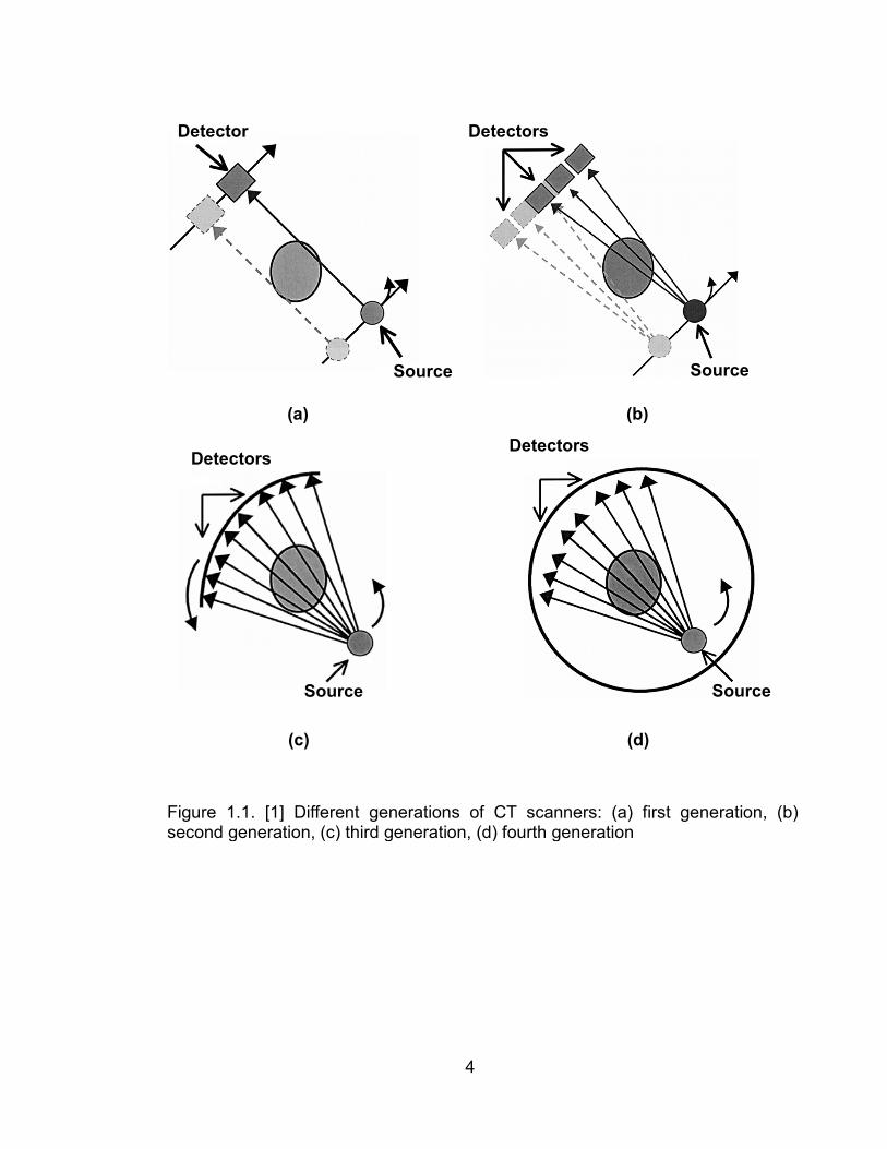
1.2.5 Fifth Generation CT Scanners

As indicated in Figure 1.2 [12], the fifth generation CT scanners are known as

EBCT, that is, electron beam CT scanner. Rather than rotating the source,

electron-beam focal point (and hence the x-ray source point) is swept

electronically, not mechanically, this motion can be much faster. The scanning

time of EBCT can be the order of milliseconds which is sufficient for cardiac

imaging. This is the mainly advantage of the EBCT and the principle reason for

the invention.

1.3 CT data measurement

In order to understand the nature of the CT data measurement, we need to first

introduce the process of x-ray attenuation briefly. X-ray attenuation is the gradual

loss of intensity of an x-ray beam when passing through the object, due to some

Figure 1.2. Fifth generation CT scanner.

6

physical process such as Photoelectric effect and Compton scattering. A CT

imaging system measures the initial intensity of the x-ray beam and its intensity

after traversing an object. By comparing the measured x-ray intensity with the

initial intensity, we can determine how much x-ray attenuation occurred during

the process. In this thesis, we consider the attenuation as a deterministic process

rather than a statistical process. The reconstructed CT images are the gray-level

representation of the distribution of object’s the x-ray attenuation coefficients in

the corresponding cross-sectional plane. The attenuation coefficients vary widely

for different maters. For a specific material, it depends on the material’s atomic

number, the x-ray intensity that transmits through it and probability of a photon

being scattered or absorbed.

Assume a narrow x-ray beam of mono-energetic photons passing through

an object and there is no scattering in this process. According to the Lambert-

Beer’s law, the attenuation can be expressed as:

𝐼𝑜 = 𝐼𝑖𝑒−𝜇𝑙 (1.1)

where 𝐼𝑜 and 𝐼𝑖 are the x-ray beam intensity after and before attenuation,

respectively. 𝜇 is the linear attenuation coefficient and 𝑙 is the length of the path.

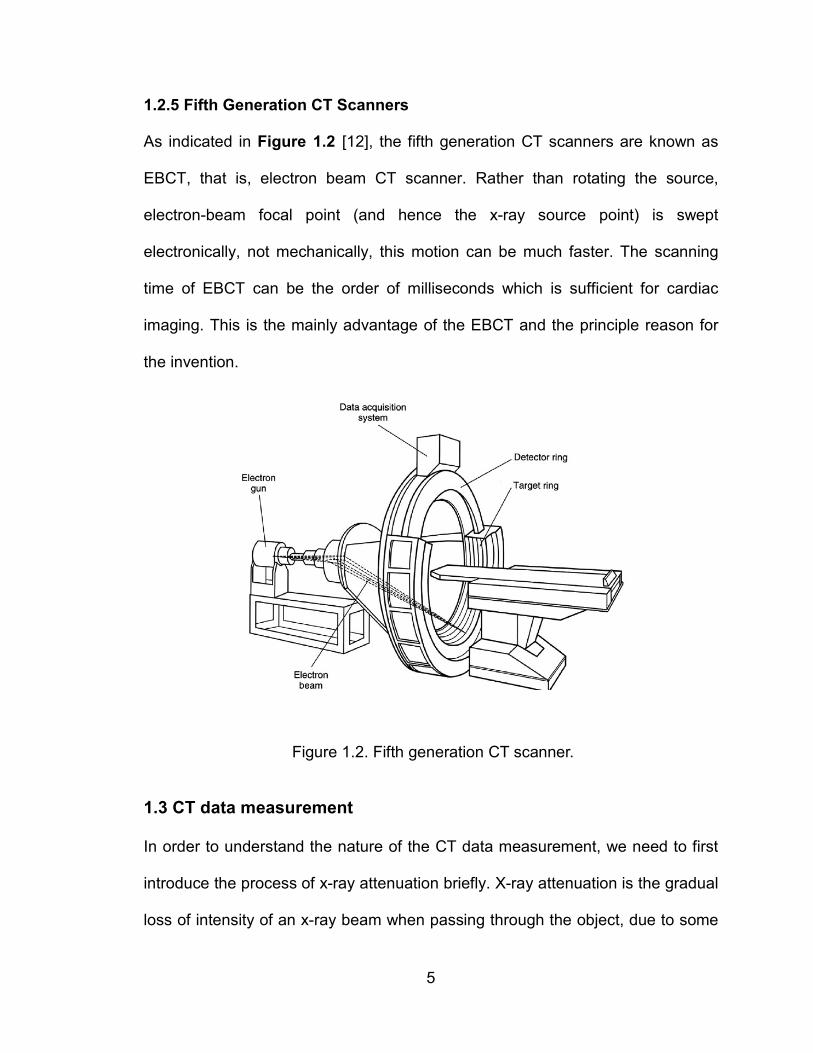
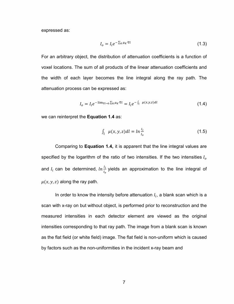
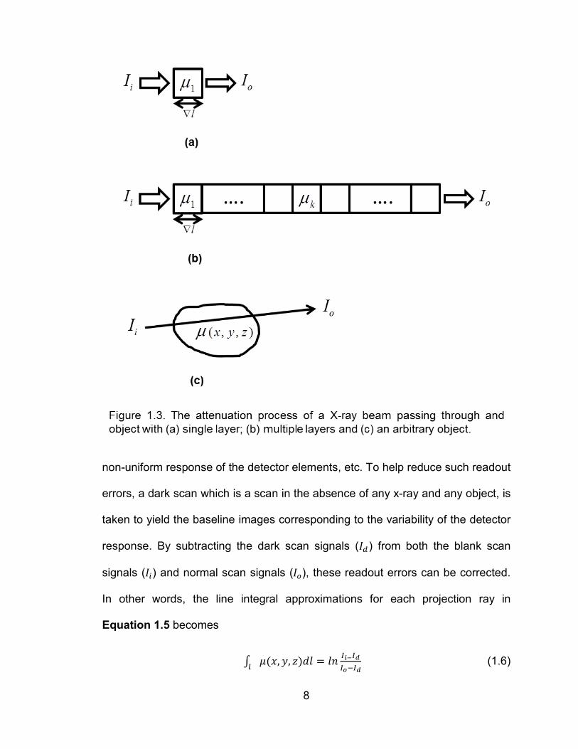
For a single layer object with constant linear attenuation coefficient 𝜇1 and width

∇𝑙, as indicated in Figure 1.3 (a), the attenuation process can be expressed as:

𝐼𝑜 = 𝐼𝑖𝑒−𝜇1∙∇𝑙 (1.2)

In the case there are multiple layers of object with various different attenuation

coefficients, as indicated in Figure 1.3 (b), the attenuation process can be

7

expressed as:

𝐼𝑜 = 𝐼𝑖𝑒−∑ 𝜇𝑘∙∇𝑙𝑘 (1.3)

For an arbitrary object, the distribution of attenuation coefficients is a function of

voxel locations. The sum of all products of the linear attenuation coefficients and

the width of each layer becomes the line integral along the ray path. The

attenuation process can be expressed as:

𝐼𝑜 = 𝐼𝑖𝑒− lim∇𝑙→0 ∑ 𝜇𝑘∙∇𝑙𝑘 = 𝐼𝑖𝑒−∫ 𝜇(𝑥,𝑦,𝑧)𝑑𝑙𝑙 (1.4)

we can reinterpret the Equation 1.4 as:

∫ 𝜇(𝑥,𝑦, 𝑧)𝑑𝑙𝑙 = 𝑙𝑛 𝐼𝑖𝐼𝑜

(1.5)

Comparing to Equation 1.4, it is apparent that the line integral values are

specified by the logarithm of the ratio of two intensities. If the two intensities 𝐼𝑜

and 𝐼𝑖 can be determined, 𝑙𝑛 𝐼𝑖𝐼𝑜

yields an approximation to the line integral of

𝜇(𝑥,𝑦, 𝑧) along the ray path.

In order to know the intensity before attenuation 𝐼𝑖, a blank scan which is a

scan with x-ray on but without object, is performed prior to reconstruction and the

measured intensities in each detector element are viewed as the original

intensities corresponding to that ray path. The image from a blank scan is known

as the flat field (or white field) image. The flat field is non-uniform which is caused

by factors such as the non-uniformities in the incident x-ray beam and

8

non-uniform response of the detector elements, etc. To help reduce such readout

errors, a dark scan which is a scan in the absence of any x-ray and any object, is

taken to yield the baseline images corresponding to the variability of the detector

response. By subtracting the dark scan signals (𝐼𝑑) from both the blank scan

signals (𝐼𝑖) and normal scan signals (𝐼𝑜), these readout errors can be corrected.

In other words, the line integral approximations for each projection ray in

Equation 1.5 becomes

∫ 𝜇(𝑥,𝑦, 𝑧)𝑑𝑙𝑙 = 𝑙𝑛 𝐼𝑖−𝐼𝑑𝐼𝑜−𝐼𝑑

(1.6)

9

there are other factors such as bad detector elements attribute to the readout

errors. We do not consider these factors in this thesis. Then the projection data

approximated by the line integrals in Equation 1.6 can be used to do

reconstruction. One thing needs to mention, the approximate projection data

calculated by Equation 1.6 is based on line integrals which considered each

detector element as an ideal point. However, the real detector element has some

size associated with it. Moreover, the line integral assumes that the photons

reach the detector along a single line. In practice, the x-ray photons passed

through the object involves some three dimensional path. These discrepancies

need to be considered when designing the system models later.

1.4 CT Image Display

The values in the displayed reconstructed images are mapped to different gray

level, which are not the attenuation coefficient that are computed based on

Equation 1.6. The Hounsfield unit (HU) which is the so called CT number is

introduced for the purpose of image display and as a uniform measurement of

pixels values in the reconstructed CT images. Because human tissues are mainly

composed of water, the HU scale is defined at a linear transformation of the

original linear attenuation coefficient measurements relative to that of water. The

CT number (HU) of the distilled water at standard pressure and temperature

(STP) is defined as zero HU. In a pixel with average linear attenuation coefficient

𝜇, the corresponding CT number (HU) is therefore defined as:

𝐻𝑈 = 1000 × 𝜇−𝜇𝑤𝑎𝑡𝑒𝑟𝜇𝑤𝑎𝑡𝑒𝑟

(1.7)

10

where 𝜇𝑤𝑎𝑡𝑒𝑟 is the linear attenuation coefficient of water which is depend on

different x-ray energy levels. Form the definition in Equation 1.7, the HU does

not proportional to the original linear attenuation coefficient. We can construct

one proportional to the original attenuation coefficient by add 1000 in the right

hand side of Equation 1.7. With this definition, some typical HU values are

indicated in Table 1. The HU values of air and water are -1000 and 0,

respectively. The bone has relative large HU values range from +400 to +4000

HU. Because the lung is mainly composed of air, it has relative small HU values

range from -600 to -400 HU. The HU values of soft tissue including fat, muscle

and other organs range from -100 to +80 HU.

Because a typical CT image often includes bone, soft tissue and water,

the large dynamic range of the image makes it difficult to observe finer details on

the display. These CT numbers are then transformed to gray level images for the

purpose of display. This defines a display window with average window level 𝑤𝑙

and window width 𝑤𝑤 . The window level 𝑤𝑙 represents the central HU value

within the window. The window width 𝑤𝑤 covers the HU of interest. Once 𝑤𝑙 and

𝑤𝑤 are determined, the maximum and minimum thresholds of HU values for gray

level mapping can be determined (Figure 1.4). CT numbers outside this range

are displayed as either black or white. The gray level of a specific pixel within the

window is linearly transformed to 0-255.

Because human vision can only differentiate about 40 different gray levels,

the selection of window level and window width enables displaying anatomical

features of different local parts in a reconstructed image hence helps determine

11

the nature of possible pathologies. Figure 1.5 illustrates the effect of different

window level and window width selections on the image display. (a) and (b) are

same reconstructed images but displayed with different window level and window

width. We can see that with a smaller window level and window width (𝑤𝑙 =

200 𝐻𝑈,𝑤𝑤 = 400 𝐻𝑈), more small details can be seen clearly in (a).

1.5 Thesis Organization

The goal of image reconstruction is to approximate the attenuation map of the

original object. As shown in Section 2.1, CT imaging process can be modeled as

a linear system 𝑊𝑓 = 𝑝 . 𝑓 is the reconstructed image, 𝑝 is the measured

projection data and 𝑊 is the system matrix. Each element in the system matrix 𝑊

quantifies the relative contribution of the specific pixel to the specific projection

12

ray. In order to calculate the system matrix elements, we have to choose a model

which is the so called system model or projection/backprojection model. The

projection/backprojection model is critical to both the reconstruction accuracy and

the efficiency of the iterative reconstruction algorithm. The ultimate goal of

choosing a projection/backprojection model is to select a model that is accurate

Figure 1.5. Same image with different display window level and window width. Window level and window width in (a) are 200 HU and 400 HU, respectively. Window level and window width in (b) are 550 HU and 500 HU, respectively.

(a) (b)

13

enough to reconstruct the original attenuation map while computational efficiency

enough to perform the reconstruction algorithm. In Section 2, we will first

introduce different models such as the pixel-driven model (PDM), ray-driven

model (RDM), area integral model (AIM) and distance-driven model (DDM). We

proposed an improved distance-driven model (IDDM) after the analysis of

different system models. In order to demonstrate the reasonability of the

proposed IDDM, we compare the different system models by theoretical analysis

and experiments that employ the projection and backprojection operations

separately. In Section 3, we will discuss the iterative reconstruction (IR)

algorithms for solving the linear system. The IR algorithms in medical imaging

field can be categorized into two major groups, namely the algebraic and

statistical algorithms. In this work, we focus on the algebraic reconstruction

algorithms. In particular, we introduce the algebraic reconstruction technique

(ART) and simultaneous algebraic reconstruction technique (SART). In order to

verify the analysis in Section 2 and compare different system models in a more

practical way, in Section 4, we will design a physical phantom to quantitatively

and qualitatively compare the AIM, DDM and IDDM based methods assuming a

typical fan-beam geometry. Finally, in Section 5, we will conclude the thesis.

14

2. System Models

2.1 Representation as a Linear System

Many imaging system, such as CT scanners can be modeled by the following

linear equations [13]:

𝑊𝑓 = 𝑝, (2.1)

where 𝑝 ∈ 𝑃 represents projection data, 𝑓 ∈ 𝐹 represents an unknown image,

and the non-zero system matrix 𝑊 ∶ 𝐹 → 𝑃 is a projection operator. Based on the

forms of 𝑓 and 𝑝, this linear system model can be classified into three category:

continuous-continuous model where 𝑓 and 𝑝 are functions, continuous-discrete

model where 𝑓 is a function and 𝑝 is a vector, and discrete-discrete model where

𝑓 and 𝑝 are vectors, 𝑃 and 𝐹 are the corresponding vector spaces. For practical

applications, the discrete-discrete model is assumed in this thesis.

For the two-dimensional (2D) case, an image can be discretized by

superimposing a square grid on the image. Usually 𝑓 is assumed as constant in

each grid cell, which is referred to as a pixel. As a result, we have a 2D digital

image 𝑓 = �𝑓𝑖,𝑗� ∈ 𝑅𝐼 × 𝑅𝐽 , where the indices 1 ≤ 𝑖 ≤ 𝐼 , 1 ≤ 𝑗 ≤ 𝐽 are integers.

Define

𝑓𝑛 = 𝑓𝑖,𝑗, 𝑛 = (𝑖 − 1) × 𝐽 + 𝑗, (2.2)

with 1 ≤ 𝑛 ≤ 𝑁, and 𝑁 = 𝐼 × 𝐽, we can re-arrange the image into a column vector

𝑓 = [𝑓1¸ 𝑓2¸ … ¸ 𝑓𝑁 ]𝑇 ∈ 𝑅𝑁. We may use both the signs 𝑓𝑛 and 𝑓𝑖,𝑗 to denote the

image. This collection of pixels in 𝑓 represents the approximation of the original

15

attenuation map of the scanned object. The goal of image reconstruction is to

reconstruct the original attenuation map from measured projection data.

The projection data 𝑝 is usually measured by detector elements, which

implies that 𝑝 is already discrete. These original projection data collected by each

detector elements takes the form of photon counts, which is equivalent to the

signal intensity. Then we modify them by using Equation 1.6 to obtain the

projection data which is available for image reconstruction. Let 𝑝𝑚 be the 𝑚𝑡ℎ

measured datum with 𝑚𝑡ℎ ray and 𝑝 = [𝑝1¸ 𝑝2¸ … ¸ 𝑝𝑀]𝑇 ∈ 𝑅𝑀 , where 𝑀 is the

total number of rays, represents all the projection rays. Equation 2.1 can be

rewritten as

𝑝𝑚 = ∑ 𝜔𝑚𝑛𝑓𝑛𝑁𝑛=1 ,𝑚 = 1,2, … ,𝑀 (2.3)

𝜔𝑚𝑛 is the element of system matrix 𝑊 = (𝜔𝑚𝑛)𝑀×𝑁.

The system matrix 𝑊 relates the image domain to the projection domain.

More generally, the system matrix 𝑊 = (𝜔𝑚𝑛)𝑀×𝑁 has 𝑀 × 𝑁 entries, the

elements 𝜔𝑚𝑛 is called the weighting coefficient that represents the relative

contribution of the 𝑛𝑡ℎ pixel to the 𝑚𝑡ℎ measured datum. Thus, weighting

coefficients relate to each projection ray yields one row in the system matrix.

Similarly, weighting coefficients relate to each pixel yields one column in the

system matrix. The product 𝑊𝑓 in the left side of Equation 2.1 projects the

image domain to the projection domain, which is also known as the forward

projection. 𝑊𝑇𝑝 (𝑊𝑇 is the transpose or adjoint matrix of 𝑊) backprojects the

projection domain to the image domain, which is known as the backprojection

16

operation. In the iterative reconstruction methods, the projection and

backprojection operations are iteratively applied to approximate the image that

best fits the measurements according to an appropriate objective function. The

system matrix also accounts for many factors such as system geometry and the

attenuation process, etc.

In order to determine the system matrix elements, we must choose some

system models which are also called projection/backprojection models. The

system model plays an important role in both the efficiency of the iterative

reconstruction process and the reconstruction accuracy. The system model

impacts the reconstruction accuracy because the solution of Equation 2.1 is the

approximation to the measured projection data 𝑝 and the solution will be accurate

only if the system matrix itself is accurate. Furthermore, the iterative

reconstruction needs to recalculate the system matrix elements iteratively based

on the system model, which is the major computational cost of the iterative

reconstruction algorithm. So the system model also affects the performance of

efficiency. Ideally, the weighting coefficient 𝜔𝑚𝑛 should completely quantify the

contribution of the 𝑛𝑡ℎpixel to the 𝑚𝑡ℎ measured datum. Creating such a system

matrix is seemingly computational impossible. Thus, choosing a system model

have to compromise between computational complexity and accuracy. The

model should be not only accurate enough to yield acceptable approximations,

but also should be computational efficiency enough to implement the

reconstruction in an acceptable fashion.

To our best knowledge, the current projection/backprojection models can

17

be divided into three categories [14]. All of those models compromise between

computational cost and accuracy. The first is the pixel-driven model (PDM),

which is usually used in the implementations of backprojection for FBP

reconstructions [15-17]. The second is the ray-driven model (RDM), which is

used for forward projection. The state of the art is the distance-driven model

(DDM), which combines the advantages of the PDM and RDM [18, 19]. It can be

used in the projection and/or backprojection processes. Recently, a finite-

detector-based projection model was proposed for iterative CT reconstructions

by Yu and Wang [20], which was also called area integral model (AIM). This

model without any interpolation is different from all the aforementioned

projection/backprojection models and can be used in the projection and

backprojection processes. Theoretically, the AIM based method is more accurate

than DDM based method, while it is very time consuming due to the high

computing cost of the system matrix. In this thesis, we proposed an improved

distance-driven model (IDDM). Theoretically, the computational cost IDDM based

method will be as low as DDM based method and the accuracy will be as high as

AIM based method. In order to compare the different projection/backprojection

models, we first choose to compare the AIM, DDM and IDDM with PDM with

linear interpolation and RDM with linear interpolation. First of all, the PDM and

RDM are the most popular two existing models. The PDM based method with

linear interpolation is probably the most popular one for filtered backprojection,

while the RDM based method with linear interpolation or bilinear interpolation is

also widely used for iterative reconstruction. Secondly, they form a good basis for

18

comparison in the two-dimensional space in terms of the accuracy and artifacts

analysis. What’s more, these two models have a perfect duality which are

suitable to compare with other models in terms of computational and artifact

properties. Then in Section 4, we will present a more thorough comparison of

DDM, IDDM and AIM based methods assuming a typical fan-beam geometry and

ultimately demonstrate the reasonability of the IDDM based method.

We use several methods to compare the different

projection/backprojection models. The first method we employed in this section is

the comparative analysis of the performance of different

projection/backprojection models in different circumstances. For example, we will

qualitatively analyze the performance of each model when the detector elements

size are less than, comparable and more than the pixel size assuming the 2D

parallel or/and fan beam geometry. Then the result can be always extended to

the 3D circumstance. When the detector element size is larger than the pixel

size, it can also test the ability of high resolution reconstruction of each model.

This is because the reconstructed images with a pixel size smaller than the

detector element size can be views as a high resolution reconstruction compare

to the detector resolution. We will also examine the likelihood of each model to

introduce artifacts in the reconstructions. For example, we can project a uniform

disk in only one view to examine the forward projection model (especially the

PDM), backproject a uniform projection in only one direction to examine the

backprojection model (especially the RDM) and/or backproject all uniform

projection from all views to generate the pixel support to further examine the

19

trends of each model to introduce ring artifact in the reconstructions. We will see

that the DDM, IDDM and AIM are outperforms the PDM and RDM after the

qualitative analysis. Furthermore, the DDM, IDDM and AIM based methods will

be further compared through the physical experiments which will be presented in

Section 4. We will compare the reconstructions by DDM, IDDM and AIM based

methods in terms of the computational cost, image noise, spatial resolution,

Structural SIMilarity (SSIM) [21] and the ability of high resolution reconstructions.

2.2 System Models

2.2.1 Pixel-driven Model

The PDM based approach refers to the main loop is the image pixel index. This

approach is usually used in the implementations of backprojection for FBP

reconstruction [15-17]. By connecting a line from the focal spot through each

pixel center, a location of interaction on the detector is determined. A value is

obtained from the detector samples via interpolation, usually by linear

interpolation, and this value is used to update the pixel values [15-17]. The

corresponding projection is the transpose of the backproejcton operation, but

now the detector elements are updated with pixel values using similar weights.

Simple PDM based approach with linear interpolation is rarely used for projection

because it causes high-frequency artifacts [18, 22], we will explain this in this

thesis. Some more complex PDM based approach exists such as the so called

splatting method in which the analytic footprint of the pixel on the detector is pre-

calculated [23]. This approach eliminates the high frequency artifacts but at the

cost of increased computational complexity.

20

2.2.2 Ray-driven Model

The RDM based approach refers to the main loop is the detector element index.

This approach is basically used for projection operation. Usually, the weighting

coefficients in the RDM based approach can be determined in two ways. The first

one is to define the weighting coefficients as the intersection length between the

projection ray and the image pixels [24-27]. Another way is to define the

weighting coefficient by interpolation, such as the linear interpolation or bilinear

interpolation, between image pixels that lie close to the projection ray [25, 28]. In

general, it connects a line from the focal spot through the image to the detector

element centre. Then the line integral is calculated by accumulating the weighted

image pixels that are related to this projection ray. The corresponding

backprojection operation is defined as the transpose of the projection operation,

but now the image pixels are updated with the values from projection using

similar weights. Ray-driven approach is rarely used in the backprojection

because it tends to introduce high frequency artifacts [14, 18].

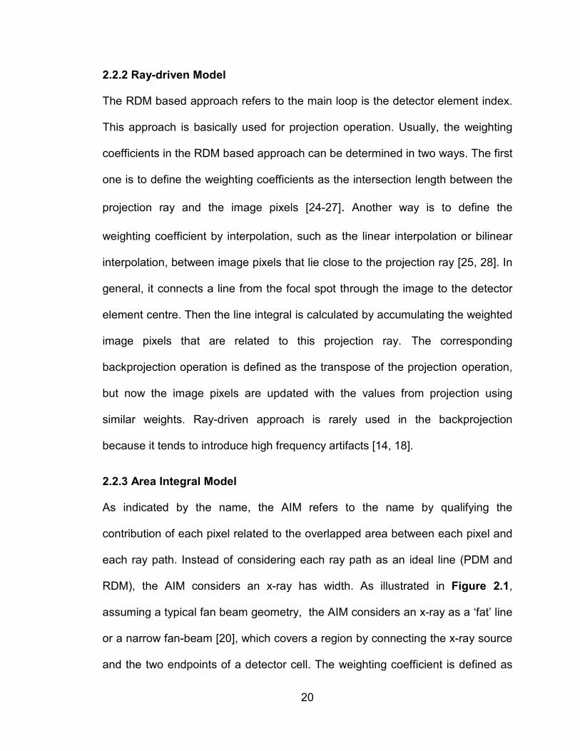
2.2.3 Area Integral Model

As indicated by the name, the AIM refers to the name by qualifying the

contribution of each pixel related to the overlapped area between each pixel and

each ray path. Instead of considering each ray path as an ideal line (PDM and

RDM), the AIM considers an x-ray has width. As illustrated in Figure 2.1,

assuming a typical fan beam geometry, the AIM considers an x-ray as a ‘fat’ line

or a narrow fan-beam [20], which covers a region by connecting the x-ray source

and the two endpoints of a detector cell. The weighting coefficient is defined as

21

the corresponding overlapped area (𝑆𝑚𝑛) which is normalized by corresponding

fan-arc length which is the product of the narrow fan beam angle (𝛾) and the

distance from the center of the pixel to the x-ray source. For the details of the

derivation, please refer to [20].

Figure 2.1. Area integral model assuming a fan beam geometry.

2.2.4 Distance-driven Model

The state of the art is the DDM, which combines the advantages of the PDM and

RDM [18, 19]. It avoids both image domain and projection domain artifacts.

Therefore, it can be used in the projection and/or backprojection processes. The

DDM considers the detector cell and image pixel has width. In order to calculate

the normalized weighting coefficients used in the projection and backprojection,

the key is to calculate the length of overlap between each image pixel and each

γ

mnS

22

detector cell, and the normalized length of overlap will be used to calculate the

weighting coefficient. To calculate the overlapped length, we need to map all the

detector cell boundaries onto the centerline of the image row of interest. In this

case the pixel boundaries are mapped onto themselves, but the detector cell

boundaries are mapped onto the center line of each row of interest. One can also

map all pixel boundaries in an image row of interest onto the detector, or map

both sets of boundaries onto a common line. In Figure 2.2, we analyze this in a

typical 2D fan beam geometry, we map the two boundaries of each detector cell

onto the centerline of the image row of interest. The two boundary locations

(sample locations) of 𝑛𝑡ℎ pixel are represented by 𝑥𝑛 and 𝑥𝑛+1 . The two

intersection locations (destination locations) between the centerline of the image

row of interest and the two boundaries of the 𝑚𝑡ℎ ray are represented by 𝑦𝑚 and

𝑦𝑚+1 . Based on these boundaries, we can calculate the overlapped length

between each image pixel and each detector cell and define the weighting

coefficient used in projection and backprojection by applying the normalized

distance-driven kernel operation (Equation A.2), and the corresponding

weighting coefficient is defined in Equation A.3. For the details of the DDM,

please refer to [14]. The 2D fan beam geometry DDM can be extended to 3D

cone-beam geometries by applying the distance-driven approach both in the in-

plane direction and in the z direction, resulting in two nested loops. Instead of

using the overlapped length between each pixel and each detector cell, the

overlapped area between each voxel and each detector cell are used to calculate

23

the weighting coefficients. For the 3D cone beam geometry, the computational

cost is much higher than the 2D case.

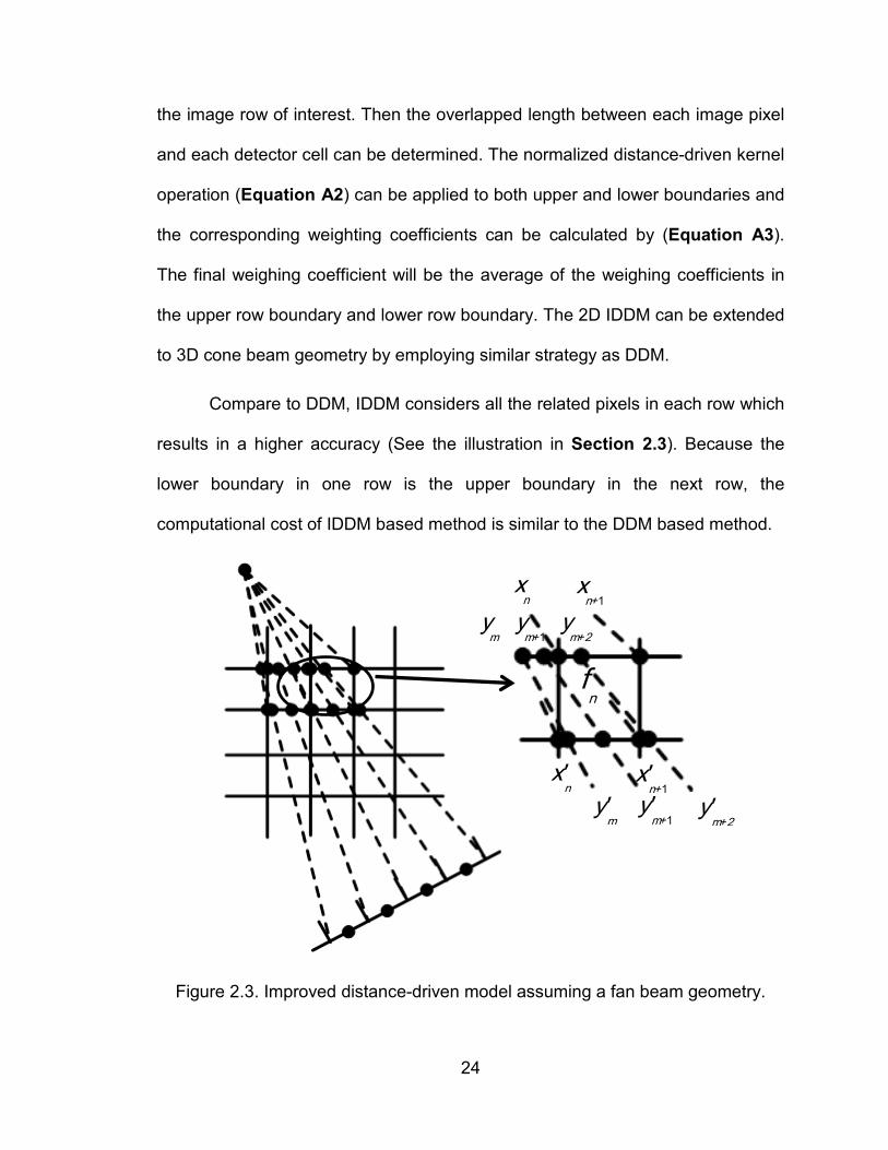
2.2.5 Improved Distance-driven Model

The IDDM also considers the x-ray has width. In order to compute the weighting

coefficient, instead of mapping the x-ray to the center line of the image row of

interest, we map the x-ray to the upper and lower boundaries of the row of

interest. In each boundary, similar way as DDM was used to compute the

weighting coefficient, the ultimate weighting coefficient is the average of the

weighting coefficients computed in the upper and lower boundaries. As illustrated

in Figure 2.3, assuming a typical 2D fan beam geometry, the two boundaries of

each detector cells are uniquely mapped onto the upper and lower boundaries of

Figure 2.2. Distance-driven model assuming a fan beam geometry.

xn+1

ym y

m+1 y

m+2

fn

xn

24

the image row of interest. Then the overlapped length between each image pixel

and each detector cell can be determined. The normalized distance-driven kernel

operation (Equation A2) can be applied to both upper and lower boundaries and

the corresponding weighting coefficients can be calculated by (Equation A3).

The final weighing coefficient will be the average of the weighing coefficients in

the upper row boundary and lower row boundary. The 2D IDDM can be extended

to 3D cone beam geometry by employing similar strategy as DDM.

Compare to DDM, IDDM considers all the related pixels in each row which

results in a higher accuracy (See the illustration in Section 2.3). Because the

lower boundary in one row is the upper boundary in the next row, the

computational cost of IDDM based method is similar to the DDM based method.

Figure 2.3. Improved distance-driven model assuming a fan beam geometry.

fn

xn x

n+1

y'm y'

m+1 y'

m+2

ym y

m+1 y

m+2

x'n x'

n+1

25

2.3 Comparative Analysis of Different Models

Before we compare the different models with simulated and/or physical

experiments, we will qualitatively analyze the performance of different

projection/backprojection models in different circumstances. We will qualitatively

analyze the performance of each model in terms of accuracy, the ability of high

resolution reconstruction and the likelihood of introducing artifacts. We will

analyze the accuracy and the ability of high resolution reconstruction of each

model (PDM, RDM, AIM, DDM and IDDM) assuming a 2D parallel beam

geometry. Similar results can be obtained in the fan beam geometry and the

results in 2D cases can be always extended to the 3D cases. We will analyze the

performance of each model when the detector elements size are less than,

comparable and more than the pixel size. When the detector element size is

larger than the pixel size, it can also test the ability of high resolution

reconstruction of each model. This is because the reconstructed images with a

pixel size smaller than the detector element size can be viewed as high

resolution reconstruction compare to the detector resolution. We will analyze this

by taking a case where the image consists of only one row and projection data

consists of only one direction. In each case, the image pixel size is fixed while

the detector element size is keep changing. The results can be extended to the

more general case with multiple rows in the image domain and multiple views in

the projection domain.

26

2.3.1 Pixel-driven Model

In PDM, each pixel corresponds to a ray during projection and backprojection.

Each ray determines a location of interaction on the detector. By using linear

interpolation the image pixel values are updated in the backprojection process.

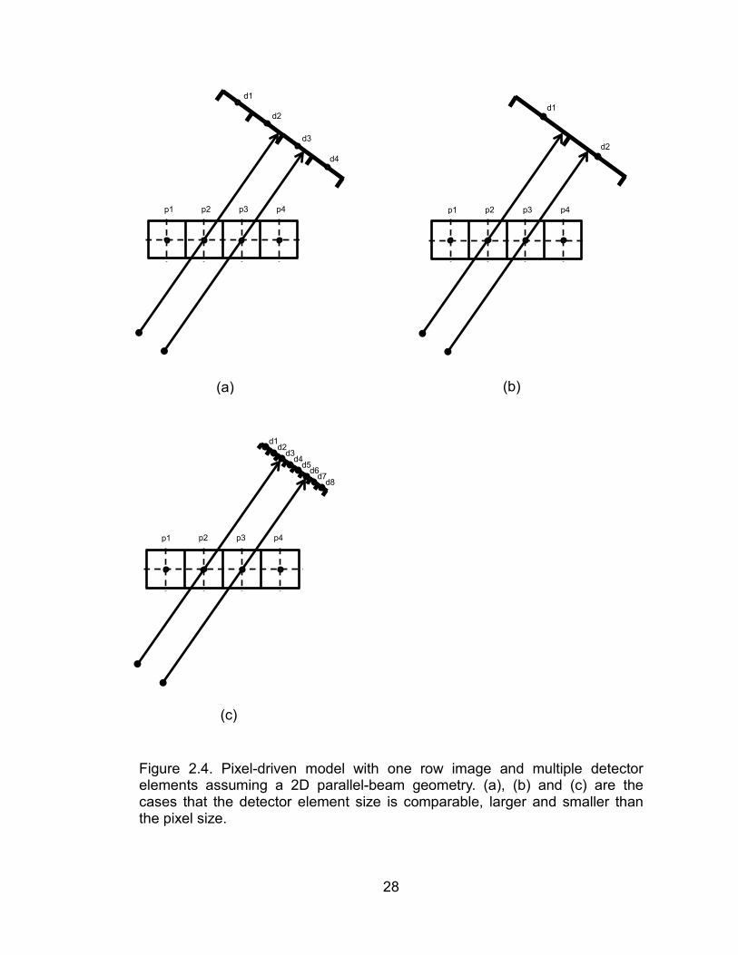
Similar weights are used to update the projection values of each ray in the

projection process. Figure 2.4 shows the PDM in three circumstances assuming

a 2D parallel geometry. In each circumstance, there is one row in the image

domain and multiple detector elements in a specific direction. The drawback of

PDM in the projection process is that it is not accurate enough and introduces

high frequency artifacts because some detector elements are updated more than

their neighbors. Figure 2.4 (a), (b) and (c) are the cases that the detector

element sizes are comparable, larger and smaller than the pixel size,

respectively. In each case, we take two rays passing through pixel number two

and three (p2, p3). For (a) which the pixel size is comparable with the detector

element size, each detector element was interacted with about one pixel ray path.

This can be viewed as each detector element was sampled about only once. The

likelihood of the detector elements are updated more than their neighbors is

small. But in the fan beam geometry, some detector elements might be updated

more than their neighbors because the pixel ray path is not always perpendicular

to the detector and this might result in some pixel ray paths interact with each

detector elements ununiformly. This might be result in the fan beam geometry

less inaccurate and more likely to introduce artifacts in the projection process

compare to the parallel beam geometry in this case. For (b) which the pixel size

27

is smaller than the detector element size, each detector element was interacted

with more than one pixel ray path in each row. The likelihood of the detector

elements are updated more than their neighbors is very small. In this case, the

performance of pixel-driven method should be better both for the parallel and the

fan beam geometry. For (c) which the pixel size is larger than the detector

element size, some detector elements have no interaction with the pixel ray path.

This will result in some detector elements are updated more than their neighbors

and even have some zero gaps for some detector elements, and finally degrade

the accuracy and introduce artifacts. In order to show this analysis, some

experiments are shown in Section 2.4. In summary, the larger the detector size

is (compare to the pixel size), the pixel-driven method is more likely to have a

better performance.

2.3.2 Ray-driven Model

In the RDM, each detector element determines a ray path by connecting the focal

spot to a point on the detector element (usually center). Then an interaction of

location is determined in the image row, and the detector element is updated with

values from image pixels by using interpolation methods such as linear or bilinear

methods. Similar weights are used in the backprojection process to update the

image pixels with values from detector elements. The drawback of the ray-driven

method is that it is not accurate enough and tends to introduce high frequency

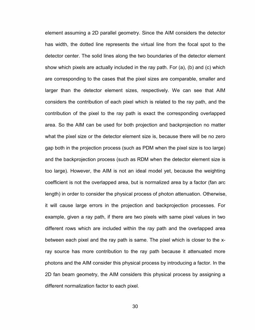
artifacts when applied to the backprojection process. Figure 2.5 shows the ray-

driven model in three cases with one row image and one detector element

assuming a 2D parallel geometry. The dotted lines along the two boundaries of

28

(a) (b)

Figure 2.4. Pixel-driven model with one row image and multiple detector elements assuming a 2D parallel-beam geometry. (a), (b) and (c) are the cases that the detector element size is comparable, larger and smaller than the pixel size.

p1 p2 p3 p4

d3 d4

d1 d2

p1 p2 p3 p4

d1

d2

(c)

d3 d4

d2 d1

d5 d6

d7 d8

p1 p2 p3 p4

29

the detector element show which pixels are actually included in the ray path. For

(a) which the pixel size is comparable with the detector element size, the dotted

line covers two related pixels (p2, p3) and the ray path (solid line) also passes

through two pixels (p2, p3). All the related pixels are counted for the projection in

this ray. Similar situation exist in (c) which the pixel size is larger than the

detector element size. The ray-driven model based projection process in these

two cases should be good enough. But the irregular contributions of the detector

elements to the image pixels still cause high frequency artifacts in the

backprojection process. For (b) which the pixel size is smaller than the detector

element size, the dotted line covers all the four pixels while the ray path (solid

line) only passes through two pixels (p2, p3). This will result the ray-driven

method less inaccurate in the projection process because some pixels’

contribution are omitted. There are also zeros gaps during backprojection which

finally introduces high frequency artifact. In sum, the smaller the detector size is

(compare to the pixel size), the better the ray-driven method is.

2.3.3 Area Integral Model

The AIM refers to the name by determining the contribution of each pixel related

to the overlapped area between each pixel and each ray path. The AIM

considers an x-ray as a ‘fat’ line which has a width. For the parallel geometry, the

weighting coefficient can be viewed as the ratio of the overlapped area and the

distance from the pixel center to the x-ray source because the normalization by

the fan-arc length becomes a constant which is the detector element length.

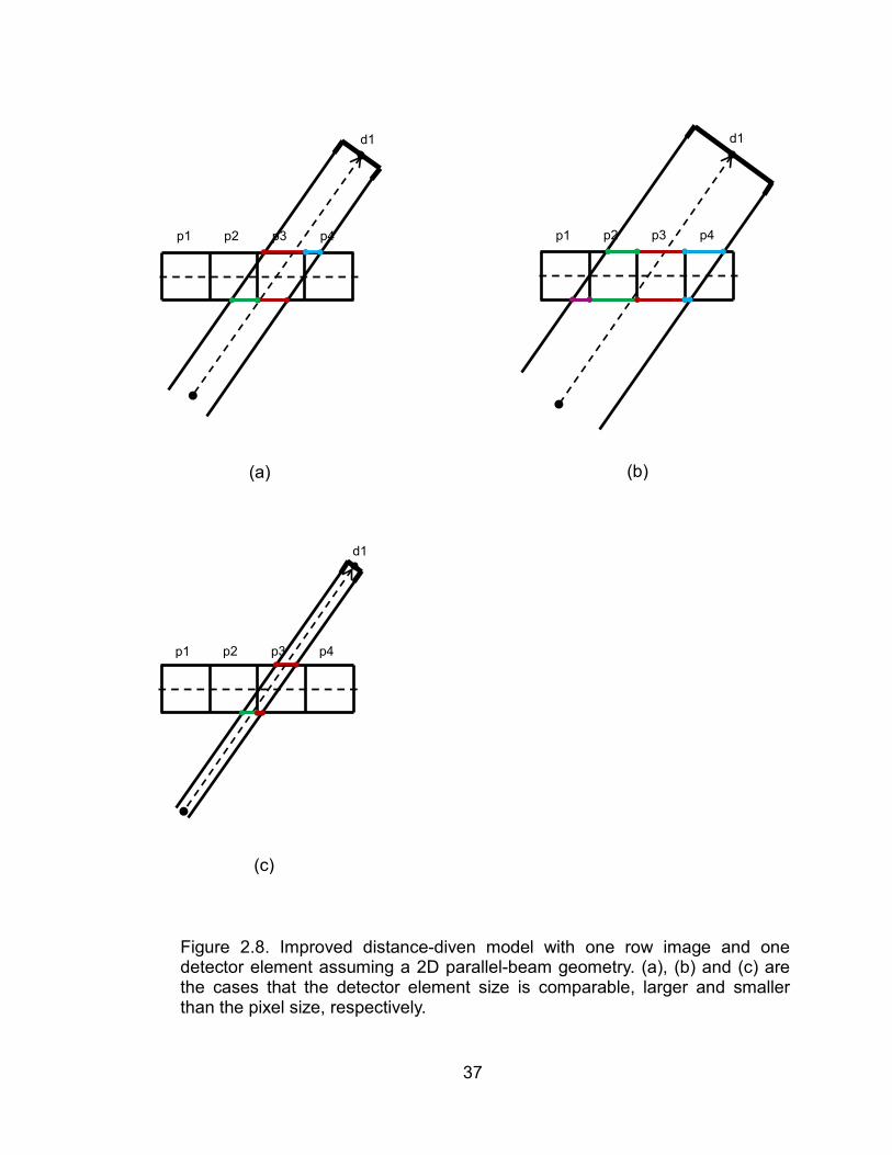
Figure 2.6 shows the AIM in three cases with one row image and one detector

30

element assuming a 2D parallel geometry. Since the AIM considers the detector

has width, the dotted line represents the virtual line from the focal spot to the

detector center. The solid lines along the two boundaries of the detector element

show which pixels are actually included in the ray path. For (a), (b) and (c) which

are corresponding to the cases that the pixel sizes are comparable, smaller and

larger than the detector element sizes, respectively. We can see that AIM

considers the contribution of each pixel which is related to the ray path, and the

contribution of the pixel to the ray path is exact the corresponding overlapped

area. So the AIM can be used for both projection and backprojection no matter

what the pixel size or the detector element size is, because there will be no zero

gap both in the projection process (such as PDM when the pixel size is too large)

and the backprojection process (such as RDM when the detector element size is

too large). However, the AIM is not an ideal model yet, because the weighting

coefficient is not the overlapped area, but is normalized area by a factor (fan arc

length) in order to consider the physical process of photon attenuation. Otherwise,

it will cause large errors in the projection and backprojection processes. For

example, given a ray path, if there are two pixels with same pixel values in two

different rows which are included within the ray path and the overlapped area

between each pixel and the ray path is same. The pixel which is closer to the x-

ray source has more contribution to the ray path because it attenuated more

photons and the AIM consider this physical process by introducing a factor. In the

2D fan beam geometry, the AIM considers this physical process by assigning a

different normalization factor to each pixel.

31

Figure 2.5. Ray-driven model with one row image and one detector element assuming a 2D parallel-beam geometry. (a), (b) and (c) are the cases that the detector element size is comparable, larger and smaller than the pixel size.

p1 p2 p3 p4

d1

p1 p2 p3 p4

d1

p1 p2 p3 p4

d1

(a)

(c)

(b)

32

The normalization factor is the arc length which is the product of the distance

from the source to the pixel center and the fan angle of the ray path. In the 2D

parallel geometry, the normalization factor for each pixel if the distance from the

pixel center to the x-ray source. This approximate normalization factor will

improve the accuracy and reduce the artifacts. The computational cost of AIM

based method will be high because the computation of the overlapped area and

the normalization factor needs many multiplication operations. In sum, the AIM

can be used in projection and backprojection processes no matter what the

detector element and the pixel sizes are. Although the computation cost of AIM is

high, its accuracy will be high.

2.3.4 Distance-driven Model

The DDM considers the x-ray has a width. In order to calculate the normalized

weighting, DDM needs to calculate the overlapped length between each image

pixel and each detector cell and the weighting coefficient will be used in

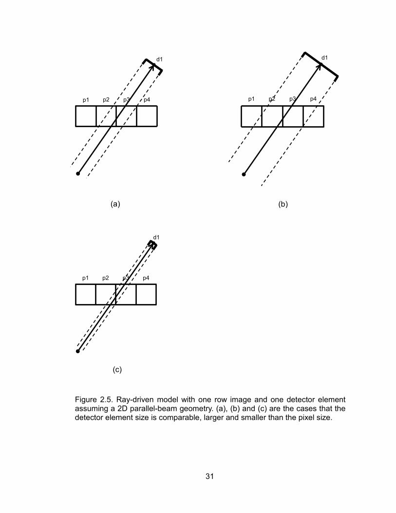
projection and backprojection. Figure 2.7 shows the DDM with one row image

and one detector element assuming a 2D parallel geometry. (a), (b) and (c) are

the cases that the detector element size is comparable, larger and smaller than

the pixel size, respectively. For each case, DDM might omit some pixels’

contribution. For example, for (a) which the detector element size and the pixel

size are comparable, there are three pixels (p2, p3, p4) related to the ray path.

However, DDM only considers the contributions of p2 and p3. It omits the

contribution from p4 but regard the p3 as a full contribution which is not exactly

the case. Similar phenomenon exists in (b) and (c). We will see that IDDM will

33

Figure 2.6. Area integral model with one row image and one detector element assuming a 2D parallel-beam geometry. (a), (b) and (c) are the cases that the detector element size is comparable, larger and smaller than the pixel size.

p1 p2 p3 p4

d1

p1 p2 p3 p4

d1

(a)

(c)

(b)

p1 p2 p3 p4

d1

34

overcome this drawback. In case (a), the performance of DDM is comparable

with RDM in the projection process and with PDM in the backprojection process.

However, the DDM will outperforms PDM or/and RDM in cases (b) or/and (c). For

(b) which the detector element size is larger than the pixel size, all the four pixels

are related to the ray path. DDM considers the contributions of three pixels (p2,

p3 and p4), but the RDM only considers the contributions of two pixels (p2, p3).

Furthermore, there is no zero gap in the backprojection process for the DDM.

However, the RDM is more likely generate zero gap in the backprojection

process in this case. The DDM outperforms the RDM both in the projection and

backprojection processes in this case. For (c) which the detector element size is

smaller than the pixel size, there is no zero gap in the backprojection process for

DDM. The DDM outperforms the PDM both in the projection and backprojection

processes in this case. In sum, DDM combines the advantages of the PDM and

RDM. It avoids both image domain and projection domain artifacts. It can be

used in the projection and/or backprojection processes no matter what the

detector element and the pixel sizes are. Theoretically, DDM is less accurate

than the AIM, but the computational cost of DDM is low.

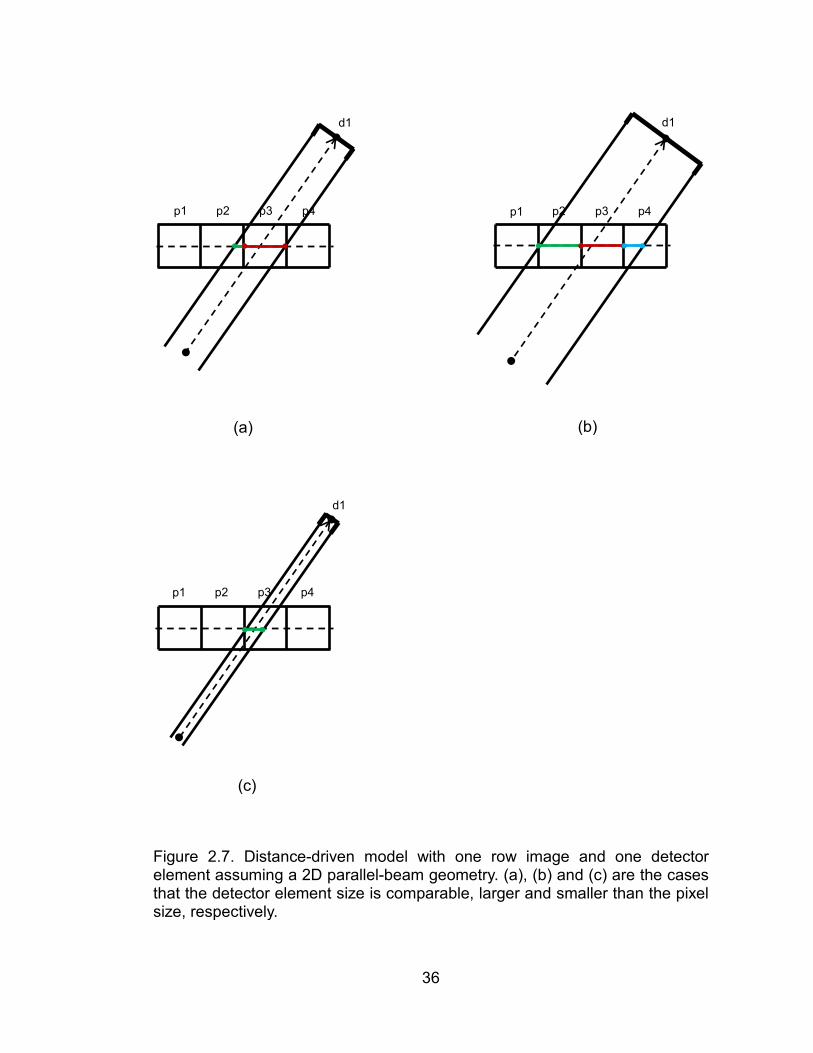
2.3.5 Improved Distance-driven Model

The IDDM also considers the x-ray has width. Figure 2.8 shows the IDDM with

one row image and one detector element assuming a 2D parallel geometry. (a),

(b) and (c) are the cases that the detector element size is comparable, larger and

smaller than the pixel size, respectively. For each case, like AIM, IDDM

considers each related pixel’s contribution to the ray path. For example, for (a)

35

which the detector element size and the pixel size are comparable, there are

three pixels (p2, p3, p4) related to the ray path. Unlike DDM, IDDM considers the

contribution of p4 and didn’t regard the p2 as a full contribution. Similar in (b) and

(c), the IDDM approach accomplish this in a more elegant way. Because the

lower boundary in one row is the upper boundary in next row, the computational

cost of IDDM approach will be as low as DDM approach. In sum, IDDM approach

can be used in the projection and/or backprojection processes no matter what

the detector element and the pixel sizes are. Theoretically, the computation cost

of IDDM approach will be as low as DDM approach, but the accuracy will be as

high as AIM.

2.4 Experimental Analysis

We will examine the above analysis by experiments with different system models

assuming a typical fan beam geometry. We will do the experiments with different

pixel sizes and detector element sizes to test different system models. For

example, we can project a uniform disk in only one view to examine the forward

projection model (especially the PDM), backproject a uniform projection in only

one direction to examine the backprojection model (especially the RDM) and/or

backproject all uniform projection from all views to generate the pixel support to

further examine the trends of each model to introduce ring artifact in the

reconstructions.

36

Figure 2.7. Distance-driven model with one row image and one detector element assuming a 2D parallel-beam geometry. (a), (b) and (c) are the cases that the detector element size is comparable, larger and smaller than the pixel size, respectively.

p1 p2 p3 p4

d1

p1 p2 p3 p4

d1

p1 p2 p3 p4

d1

(a)

(c)

(b)

37

Figure 2.8. Improved distance-diven model with one row image and one detector element assuming a 2D parallel-beam geometry. (a), (b) and (c) are the cases that the detector element size is comparable, larger and smaller than the pixel size, respectively.

p1 p2 p3 p4

d1

p1 p2 p3 p4

d1

p1 p2 p3 p4

d1

(a)

(c)

(b)

38

2.4.1 Projection of a Uniform Disk

As we discussed in Section 2.3, the performance of PDM based approach is bad

especially when the detector element size is smaller than the image pixel size. In

order to demonstrate this phenomenon and compare the performance with AIM,

DDM and IDDM based approach, we project a uniform disk in one direction (such

as 126 degrees) with the detector element size is smaller, comparable and larger

than the image pixel size, respectively. Because the DDM and IDDM need to

change the projection axis in 45 degrees directions during projection and/or

backprojection, which the approximation errors are large in these directions, we

also show the experiments in these directions. Figure 2.9 shows the projection in

126 degrees direction with the detector element size is larger than the image

pixel size. From the first to the fourth rows, the system models are PDM with

linear interpolation, AIM, DDM and IDDM. In each row, figure in the right side is

the corresponding magnified region within the yellow square in the left side. We

can see that the performance of PDM based approach is fairly good in this case.

There are no vibrations even in the magnified figure. This is consistent with the

analysis in Section 2.3. In fact, the four models have similar performance in this

case. As the detector element size becomes comparable with the image pixel

size (Figure 2.10), the PDM based approach begins to inferior to the AIM, DDM

and IDDM based approaches. This is because the irregular weighting becomes

more apparent for the PDM based approach compare to AIM, DDM and IDDM

based approaches, which is also consistent with the analysis in Section 2.3.

From the magnified regions, we can see that the vibrations of IDDM based

39

approach are smaller than AIM based approach, they are both smaller than the

DDM based approach. This means that the AIM and IDDM based approaches

are more accurate than DDM based approach in the projection process. As the

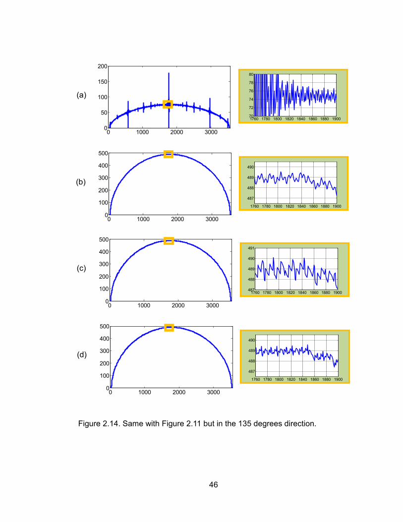
detector element size becomes larger than the image pixel size (Figure 2.11),

the irregular weighting in the PDM based approach becomes very serious and

even make this model useless. The vibrations of IDDM based approach are

further smaller than the AIM based approach, they are both smaller than DDM

based approach. The vibrations of AIM, DDM and IDDM based approaches are

barely affected by the relative image pixel sizes and the detector element sizes.

Figures 2.12, 2.13 and 2.14 are same with Figures 2.9, 2.10 and 2.11 but in the

135 degrees direction. Similar phenomena are also observed in the 125 degrees

direction. In sum, AIM, DDM and IDDM based approaches are outperform to

PDM based approach in the projection process. The AIM and IDDM based

approaches are outperforms the DDM based approach. All the three models can

be used for the projection process in different cases.

2.4.2 Backprojection of a Uniform Projection

As we discussed in Section 2.3, the RDM based approach tends to introduce

artifacts when applied to the backprojection especially when the detector element

size is larger than the image pixel size. In order to demonstrate this phenomenon

and compare the performance with AIM, DDM and IDDM based approaches, we

backproject a uniform projection in a specific direction (such as 126 and 135

degrees) with the detector element size is smaller, comparable and larger than

the image pixel size, respectively. Figures 2.15 and 2.17 show the

40

backprojection of a uniform projection data in 126 and 135 degrees direction.

From the first to the third columns are the cases that the detector element sizes

are larger, comparable and smaller than the image pixel sizes, respectively. From

the first to the fifth rows, the system models are RDM with linear interpolation,

RDM with bilinear interpolation, AIM, DDM and IDDM, respectively. We can see

that the performance of bakcprojection with the RDM based approach (linear and

bilinear interpolations) is very bad when the detector element size is larger than

the image pixel size (the first two images in the first column). There are apparent

zero gap during backprojection in this case just like we analyzed in Section 2.3.

The bilinear interpolation used in the RDM can not improve the poor performance

too much. When the detector element sizes are comparable with the image pixel

sizes (the first two images in the second column), the performance of RDM

based approach becomes much better. The RDM based approach with linear

interpolation shows apparent stripe-like patterns. However, the RDM based

approach with bilinear interpolation improves this stripe-like patterns a lot but at

the cost of increasing computational cost. When the detector element size is

smaller than the image pixel size (the first two images in the last column), the

performance of RDM based approach is further improved. The RDM based

approach with linear interpolation still shows some stripe-like patterns while the

bilinear interpolation approach almost eliminates the stripe-like patterns. No

matter what the sizes of the detector elements and the image pixel sizes are, the

AIM, DDM and IDDM based approaches can generate a uniform backprojection,

41

0 20 40 60 80 1000

100

200

300

400

500

50 55 60 65480

482

484

486

488

490

(a)

0 20 40 60 80 1000

500

1000

1500

2000

2500

50 55 60 652350

2360

2370

2380

2390

2400

(b)

0 20 40 60 80 1000

100

200

300

400

500

50 55 60 65480

482

484

486

488

490

(c)

Figure 2.9. Projection of a uniform disk in one direction (126 degrees) assuming a fan beam geometry with the detector element size larger than image pixel size. From (a) to (d), the system models are PDM with linear interpolation, AIM, DDM and IDDM. In each row, figure in the right side is the corresponding magnified region within the yellow square in the left side.

0 20 40 60 80 1000

100

200

300

400

500

50 55 60 65480

482

484

486

488

490

(d)

42

0 200 400 600 8000

100

200

300

400 420 440 460 480297

298

299

300

301

400 420 440 460 480486

487

488

489

490

0 200 400 600 8000

100

200

300

400

500

0 200 400 600 8000

100

200

300

400

500

400 420 440 460 480486

487

488

489

490

Figure 2.10. Same with Figure 2.9 but the detector element size is comparable with the image pixel size.

0 200 400 600 8000

100

200

300

400

500

400 420 440 460 480486

487

488

489

490

(a)

(b)

(c)

(d)

43

0 1000 2000 30000

50

100

150

200

1760 1780 1800 1820 1840 1860 1880 190060

70

80

90

0 1000 2000 30000

100

200

300

400

500

1760 1780 1800 1820 1840 1860 1880 1900

487

488

489

490

0 1000 2000 30000

100

200

300

400

500

1760 1780 1800 1820 1840 1860 1880 1900487

488

489

490

491

Figure 2.11. Same with Figure 2.9 but the detector element size is smaller than the image pixel size.

0 1000 2000 30000

100

200

300

400

500

1760 1780 1800 1820 1840 1860 1880 1900

487

488

489

490

(a)

(b)

(c)

(d)

44

Figure 2.12. Same with Figure 2.9 but in the 135 degrees direction.

0 20 40 60 80 1000

500

1000

1500

2000

2500

50 55 60 652350

2360

2370

2380

2390

2400

0 20 40 60 80 1000

100

200

300

400

500

50 55 60 65480

482

484

486

488

490

0 20 40 60 80 1000

100

200

300

400

500

50 55 60 65480

482

484

486

488

490

0 20 40 60 80 1000

100

200

300

400

500

50 55 60 65480

482

484

486

488

490

(a)

(b)

(c)

(d)

45

Figure 2.13. Same with Figure 2.10 but in the 135 degrees direction.

0 200 400 600 8000

100

200

300

400 420 440 460 480260

280

300

320

0 200 400 600 8000

100

200

300

400

500

400 420 440 460 480486

487

488

489

490

0 200 400 600 8000

100

200

300

400

500

400 420 440 460 480486

487

488

489

490

0 200 400 600 8000

100

200

300

400

500

400 420 440 460 480486

487

488

489

490

(a)

(b)

(c)

(d)

46

Figure 2.14. Same with Figure 2.11 but in the 135 degrees direction.

0 1000 2000 30000

100

200

300

400

500

1760 1780 1800 1820 1840 1860 1880 1900

487

488

489

490

0 1000 2000 30000

50

100

150

200

1760 1780 1800 1820 1840 1860 1880 190070

72

74

76

78

80

0 1000 2000 30000

100

200

300

400

500

1760 1780 1800 1820 1840 1860 1880 1900487

488

489

490

491

0 1000 2000 30000

100

200

300

400

500

1760 1780 1800 1820 1840 1860 1880 1900

487

488

489

490

(a)

(b)

(c)

(d)

47

which is outperform the RDM based approach. In order to further compare the

performance of the AIM, DDM and IDDM based methods, we plot the contour

maps of the backprojection generated by these three methods. Figures 2.16 and

2.18 show the contour maps of the last three rows in Figures 2.15 and 2.17,

respectively. A contour map is composed of contour line, which can be used to

show valleys and hills, and the steepness of slopes. A contour line can be formed

by joining points with values above a given threshold. When the lines are close

together, the magnitude of the gradient is large which means the changing rate is

fast. According to the contour plot, the performance of AIM, DDM and IDDM

based approaches are also very similar. When the detector element is larger than

the image pixel size (the first column), the contour interval for all the three

approach is smaller than the other two cases. This means the vibrations in the

backprojection are a little bit larger than the other two cases. But if we observe

carefully, we will see that the vibrations of AIM approach in each contour line are

smaller than the DDM and IDDM approach. This means the AIM approach is

more accurate than DDM and IDDM approach in the backprojection process

when the detector element size is larger than the image pixel size. When the

detector element sizes are comparable and smaller than the detector sizes

(second and third columns), for each method, there is no big difference observed

from the contour plot. That means, when the detector element size is smaller

than the image pixel size, the accuracy of the AIM, DDM and IDDM based

approaches in the backprojection will not be improved too much. In sum, AIM,

DDM and IDDM based approaches are outperform to RDM based approach in

48

the backprojection process. The AIM based approach are a little bit outperforms

the DDM and IDDM based approach when the detector element is larger than the

pixel element. All the three models can be used for the backprojection process in

different cases.

2.4.3 Pixel Support

From a practical standpoint, the extent to which a system model avoids artifacts

(ring artifact) is more important. Here we will generate the pixel support to further

compare the system models in terms of support value consistency and examine

the likelihood of introducing ring artifacts. The pixel support image is generated

by backprojecting a projection data of constant ones. The support value for the

𝑛𝑡ℎ pixel is equivalent to the sum of the 𝑛𝑡ℎ column of the system matrix. As the

source and detector rotates around the isocenter, the intersections of the fan

beam over all projection views yields a circle region. The scanner system

provides data support within the circle region because the projection data is

available within this region. There is no data support outside the region. So there

will be a step change around the boundaries of the support region in the pixel

support image. However, it is expect that there should be no large variations

within the support region for a good system model. Large variations within the

pixel support tend to generate ring artifacts in the reconstruction. Thus, we can

test the effectiveness of different system models by generating the corresponding

pixel support. Figure 2.19 shows the pixel supports with image size 512x512

assuming a fan beam geometry. From the first column to the third column are the

cases that the detector element sizes are larger, comparable and smaller than

49

Continued

50

Figure 2.16. Contour plots of the last three rows in Figure2.15.

50 100 150 200 250 300 350 400 450 500

50

100

150

200

250

300

350

400

450

500

50 100 150 200 250 300 350 400 450 500

50

100

150

200

250

300

350

400

450

500

50 100 150 200 250 300 350 400 450 500

50

100

150

200

250

300

350

400

450

500

50 100 150 200 250 300 350 400 450 500

50

100

150

200

250

300

350

400

450

500

50 100 150 200 250 300 350 400 450 500

50

100

150

200

250

300

350

400

450

500

50 100 150 200 250 300 350 400 450 500

50

100

150

200

250

300

350

400

450

500

50 100 150 200 250 300 350 400 450 500

50

100

150

200

250

300

350

400

450

500

50 100 150 200 250 300 350 400 450 500

50

100

150

200

250

300

350

400

450

500

50 100 150 200 250 300 350 400 450 500

50

100

150

200

250

300

350

400

450

500

Figure 2.15. Backprojection of a uniform projection data in 126 degrees direction assuming a fan beam geometry. From the first column to the third column are the cases that the detector element sizes are larger, comparable and smaller than the image pixel sizes, respectively. From the first row to the fifth row, the system models are ray-driven model with linear interpolation, ray-driven model with bilinear interpolation, AIM, DDM and IDDM , respectively.

51

Continued

52

50 100 150 200 250 300 350 400 450 500

50

100

150

200

250

300

350

400

450

500

50 100 150 200 250 300 350 400 450 500

50

100

150

200

250

300

350

400

450

500

50 100 150 200 250 300 350 400 450 500

50

100

150

200

250

300

350

400

450

500

50 100 150 200 250 300 350 400 450 500

50

100

150

200

250

300

350

400

450

500

50 100 150 200 250 300 350 400 450 500

50

100

150

200

250

300

350

400

450

500

50 100 150 200 250 300 350 400 450 500

50

100

150

200

250

300

350

400

450

500

50 100 150 200 250 300 350 400 450 500

50

100

150

200

250

300

350

400

450

500

50 100 150 200 250 300 350 400 450 500

50

100

150

200

250

300

350

400

450

500

50 100 150 200 250 300 350 400 450 500

50

100

150

200

250

300

350

400

450

500

Figure 2.18 Contour plots of the last three rows in Figure2.17

Figure 2.17 Same with Figure 2.15 but in the 135 degrees direction.

53

the image pixel sizes, respectively. From the first row to the fifth row, the system

models are RDM with linear interpolation, RDM with bilinear interpolation, AIM,

DDM and IDDM, respectively. We can see the severe ring artifacts from the pixel

support generated by the RDM based approaches (linear and bilinear

interpolations) when the detector element size is larger than the image pixel size

(the first two images in the first column). The bilinear interpolation used in the

RDM can not diminish the ring artifacts. When the detector element sizes are

comparable and smaller than the image pixel sizes (the first two images in the

second and third columns, respectively), the pixel support of RDM based

approach becomes much more uniform. The RDM based approach with linear

interpolation has some artifacts while the RDM based approach with bilinear

interpolation looks pretty good. No matter what the sizes of the detector elements

and the image pixel sizes are, the AIM, DDM and IDDM based approaches can

generate a uniform pixel support. In order to further compare the pixel support

and examine the ring artifact of the AIM, DDM and IDDM based methods, we plot

the contour map of the pixel support generated by these three methods. Figure

2.20 shows the contour map of the last three rows in Figure 2.19. According to

the contour plot, the performance of AIM, DDM and IDDM based approaches are

also very similar. The image support seems best when the detector element size

is comparable with the image pixel size (the second column) for the three

methods. This is probably because the artifacts are accentuated when the

detector element size is smaller than the image pixel size. The image support in

the third column (detector element size is smaller than the image pixel size) is

54

more uniform than the first column (detector element size is larger than the

image pixel size) because the contour interval in the third column is larger than

the first column. In order to further examine the vibrations of the pixel support, we

plot the line profiles of the 256𝑡ℎ row. Figure 2.21 shows the line profiles which

are corresponding to the first column in Figure 2.19, which the detector element

size is smaller than the image pixel size. We can see that the vibrations of the

RDM based approach (both for linear interpolation and bilinear interpolation) are

larger than the AIM, DDM and IDDM based approaches. There is almost no

vibrations in the AIM based approach in this case. There are smaller vibrations in

the DDM and IDDM based approaches. Once again, the high resolution

reconstruction ability of AIM based approach is better than DDM and IDDM

approaches. Figure 2.22 shows the line profiles which are corresponding to the

second column in Figure 2.19, which the detector element size is comparable

with the image pixel size. The vibrations in the RDM based approach with linear

interpolation are larger than the bilinear interpolation. There are almost no

vibrations even from the magnified regions in the AIM, DDM and IDDM based

approaches. All the three approaches outperform the RDM based approach.

Figure 2.23 shows the line profiles which are corresponding to the third column

in Figure 2.19, which the detector element size is smaller the image pixel size.

We can barely recognize the difference between the RDM based approach with

bilinear interpolation and the AIM, DDM and IDDM based approaches from the

pixel support images. Now we can clearly see that there are still small vibrations

in the image support generated by the RDM based approach when the detector

55

element is smaller than the image pixel size. There are no vibrations in the pixel

support generated by AIM, DDM and IDDM based approaches.

From the above experiments, we can clearly see that AIM, DDM and

IDDM based approaches are outperform the PDM based approach and RDM

based approaches. The AIM and IDDM based approaches have similar

performance in the projection process, which are both outperform the DDM

based approach in the projection process. The AIM based approach outperforms

the DDM and IDDM based approaches in the backprojection process when the

detector element size is larger than the image pixel size, which means that the

AIM based approach is more suitable for the high resolution reconstruction than

the DDM and IDDM based approaches. The AIM, DDM and IDDM based

approaches have similar performance in the backprojection process when the

detector element sizes are comparable and smaller than the image pixel sizes. In

Section 4, we will further compare AIM, DDM and IDDM based methods with a

physical phantom experiment in terms of the computational cost, image noise,

spatial resolution, Structural SIMilarity (SSIM) [21] and the ability of high

resolution reconstructions.

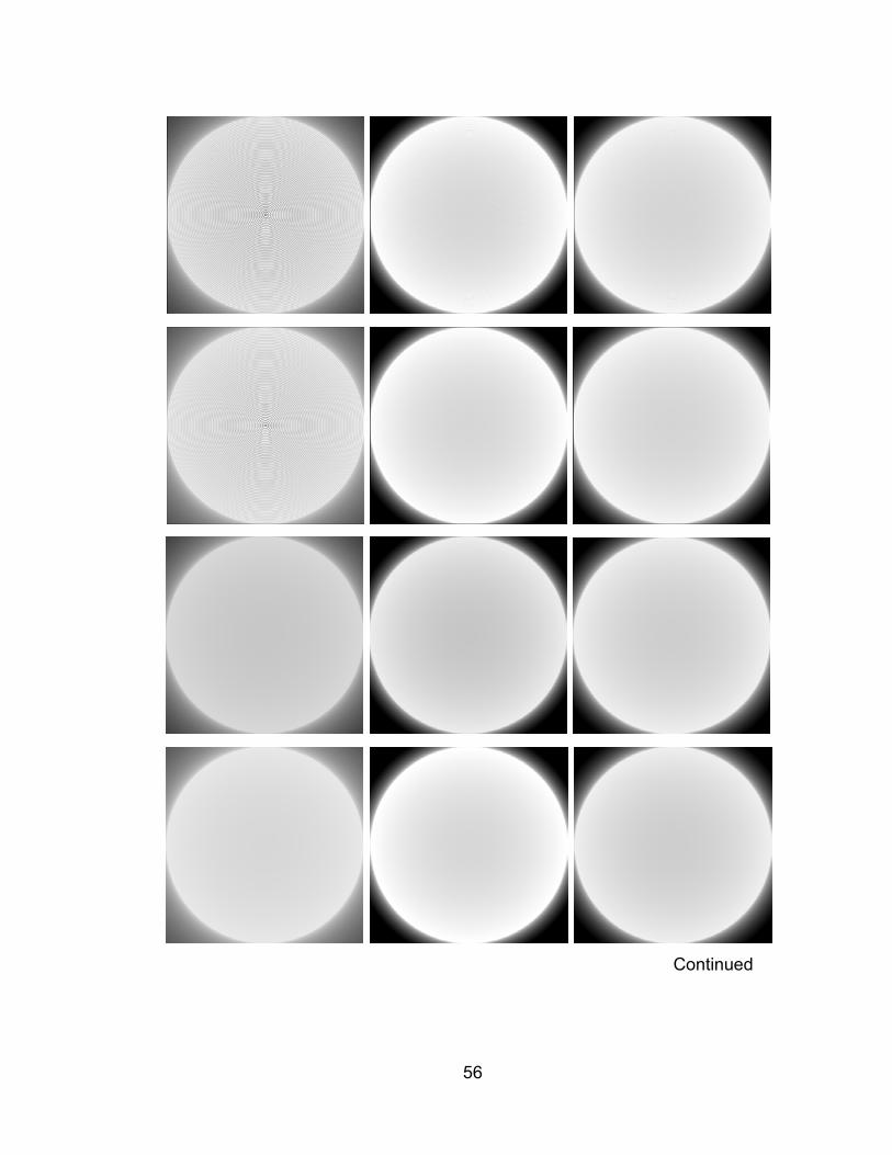
56

Continued

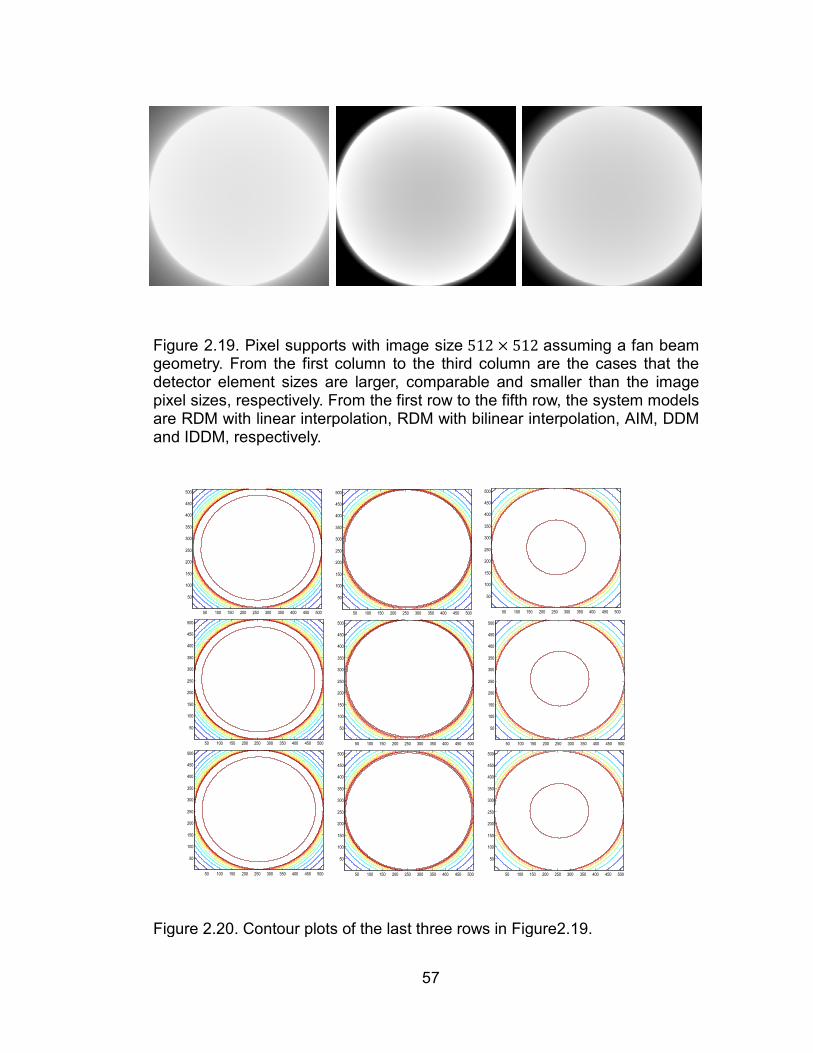
57

50 100 150 200 250 300 350 400 450 500

50

100

150

200

250

300

350

400

450

500

50 100 150 200 250 300 350 400 450 500

50

100

150

200

250

300

350

400

450

500

50 100 150 200 250 300 350 400 450 500

50

100

150

200

250

300

350

400

450

500

50 100 150 200 250 300 350 400 450 500

50

100

150

200

250

300

350

400

450

500

50 100 150 200 250 300 350 400 450 500

50

100

150

200

250

300

350

400

450

500

50 100 150 200 250 300 350 400 450 500

50

100

150

200

250

300

350

400

450

500

50 100 150 200 250 300 350 400 450 500

50

100

150

200

250

300

350

400

450

500

50 100 150 200 250 300 350 400 450 500

50

100

150

200

250

300

350

400

450

500

50 100 150 200 250 300 350 400 450 500

50

100

150

200

250

300

350

400

450

500

Figure 2.20. Contour plots of the last three rows in Figure2.19.

Figure 2.19. Pixel supports with image size 512 × 512 assuming a fan beam geometry. From the first column to the third column are the cases that the detector element sizes are larger, comparable and smaller than the image pixel sizes, respectively. From the first row to the fifth row, the system models are RDM with linear interpolation, RDM with bilinear interpolation, AIM, DDM and IDDM, respectively.

58

(a)

0 100 200 300 400 500100

150

200

250

300

350

220 240 260 280

150

200

250

300

350

0 100 200 300 400 500100

150

200

250

300

350

220 240 260 280

150

200

250

300

350

0 100 200 300 400 500200

205

210

215

220 240 260 280200.5

201

201.5

(b)

(c)

Continued

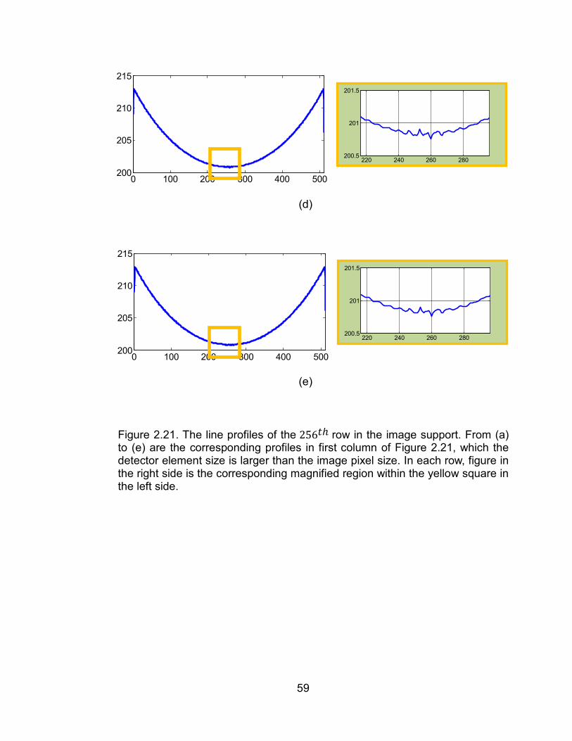
59

Figure 2.21. The line profiles of the 256𝑡ℎ row in the image support. From (a) to (e) are the corresponding profiles in first column of Figure 2.21, which the detector element size is larger than the image pixel size. In each row, figure in the right side is the corresponding magnified region within the yellow square in the left side.

0 100 200 300 400 500200

205

210

215

220 240 260 280200.5

201

201.5

0 100 200 300 400 500200

205

210

215

220 240 260 280200.5

201

201.5

(d)

(e)

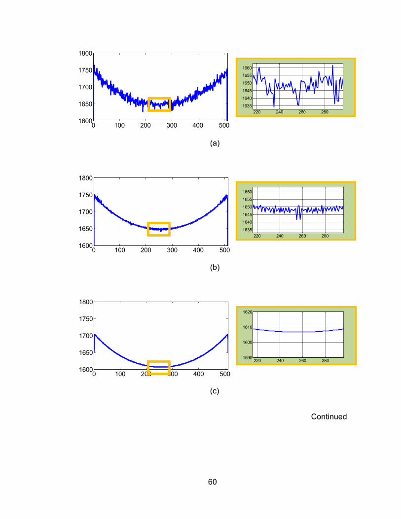
60

0 100 200 300 400 5001600

1650

1700

1750

1800

220 240 260 280

1635

1640

1645

1650

1655

1660

0 100 200 300 400 5001600

1650

1700

1750

1800

220 240 260 2801635

1640

1645

1650

1655

1660

0 100 200 300 400 5001600

1650

1700

1750

1800

220 240 260 2801590

1600

1610

1620

(a)

(b)

(c)

Continued

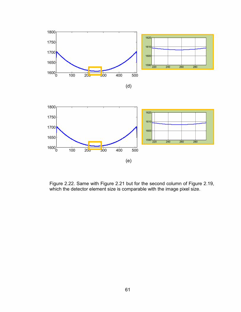
61

0 100 200 300 400 5001600

1650

1700

1750

1800

220 240 260 2801590

1600

1610

1620

0 100 200 300 400 5001600

1650

1700

1750

1800

220 240 260 2801590

1600

1610

1620

(d)

(e)

Figure 2.22. Same with Figure 2.21 but for the second column of Figure 2.19, which the detector element size is comparable with the image pixel size.

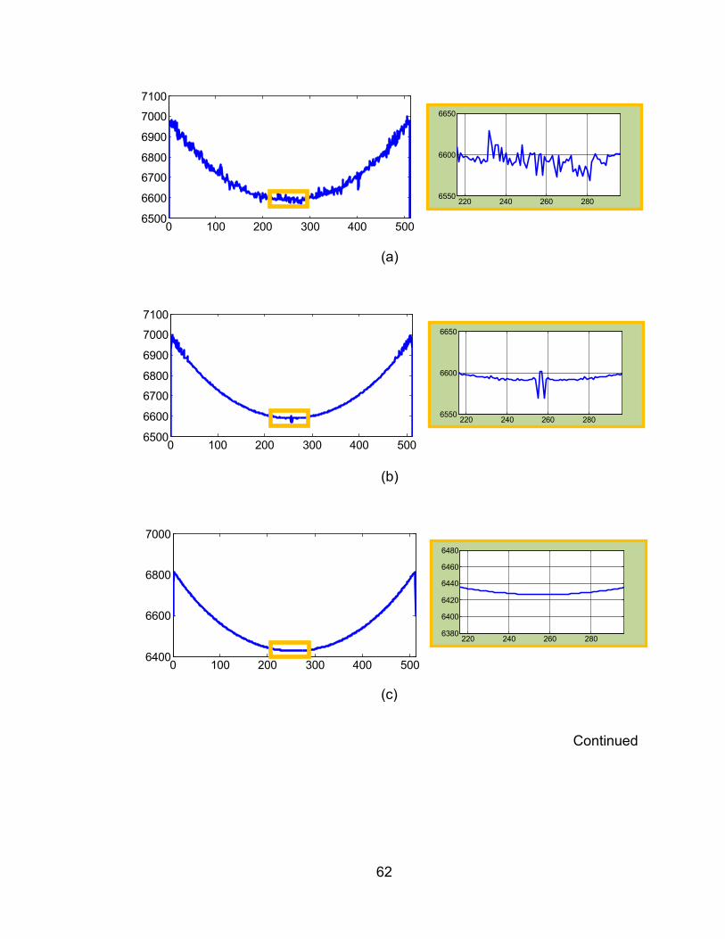
62

0 100 200 300 400 5006500

6600

6700

6800

6900

7000

7100

220 240 260 2806550

6600

6650

0 100 200 300 400 5006500

6600

6700

6800

6900

7000

7100

220 240 260 2806550

6600

6650

0 100 200 300 400 5006400

6600

6800

7000

220 240 260 2806380

6400

6420

6440

6460

6480

(a)

(b)

(c)

Continued

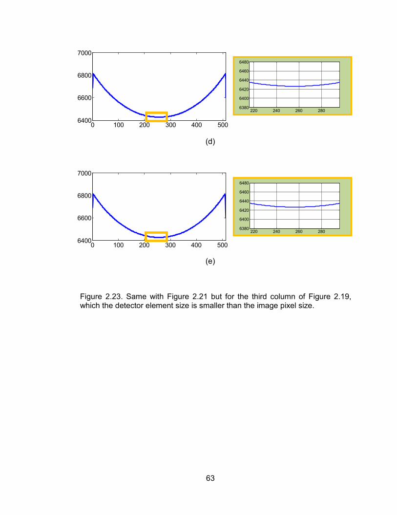
63

0 100 200 300 400 5006400

6600

6800

7000

220 240 260 2806380

6400

6420

6440

6460

6480

0 100 200 300 400 5006400

6600

6800

7000

220 240 260 2806380

6400

6420

6440

6460

6480

(d)

(e)

Figure 2.23. Same with Figure 2.21 but for the third column of Figure 2.19, which the detector element size is smaller than the image pixel size.

64

3. Iterative Image Reconstruction Algorithms

3.1 Overview

Once the system model is selected, the system matrix 𝑊 can be determined. In

order to reconstruct the object from the measured projection data, we need to

compute an approximation to 𝑓 by solving the linear system represented by

Equation 2.1. While direct methods exist for solving such a linear squares

problem, such as applying Cholesky method to the associated normal equation

of the linear square problem given by 𝑊𝑇𝑊𝑓 = 𝑊𝑇𝑝. However, the dimension of

the system matrix 𝑊 prevents the direct methods from being practical. Rather

than using the whole system matrix, the iterative methods use one or multiple

rows of the system matrix at a time to solve the linear system equation iteratively.

The basic idea of the iterative reconstruction (IR) methods is to minimize the

error between the computed projection data and the measured projection data

iteratively. Once the stopping criteria are satisfied, the current estimate of the

solution will be regarded as the reconstruction.

The IR algorithms used for image reconstruction can be categorized into

two major groups, namely the algebraic and statistical algorithms. Representative

among the algebraic reconstruction algorithms are algebraic reconstruction

technique (ART) [10, 29, 30] and simultaneous algebraic reconstruction

technique (SART) [5, 31, 32]. The mainly difference between the ART and the

SART is the numbers of rays that are considered at a time. The ART algorithm

considers one projection ray at a time while SART considers all the projection

rays in terms of views at a time. When the projection rays from partial views are

65

considered at a time, the SART becomes the ordered subset simultaneous

algebraic reconstruction technique (OS-SART). The convergence speed is

greatly accelerated when the OS-SART is used. The convergence of the SART

or/and OS-SART type algorithms are proved by J. Ming and G. Wang [32]

assuming a non-negative real space. The assumption of the non-negative real

space is reasonable because the linear coefficients are always non-negative in

the true CT applications. The statistical algorithms differ from the algebraic

algorithms in that they attempt to look for the solution by some statistical

approach. One of the most successful statistical reconstruction algorithms is the

maximum likelihood expectation-maximization (ML-EM) algorithm [33-35], which

is also called the Richardson-Lucy algorithm or Lucy-Richardson algorithm,

because Richardson and Lucy first developed this algorithm for image deblurring

applications in 1972 and 1974 [36, 37]. In the ML-EM algorithm, the objective

function is not a least squares function but a likelihood function, which is the joint

probability density function of some random variables (such as Poisson random

variables). Then the solution (reconstructed image) can be obtained by maximize

the likelihood function. Although the convergence speed of the EM-ML algorithm

is slow, this algorithm is guaranteed to converge to the maximum likelihood [38].

However, the reconstructed image obtained by maximizing the likelihood

objective function usually is not of the best visual quality. In practice, an

empirically selected number of iterations are usually used to stop the iteration for

most of the clinical applications. In this work, we only focus on the algebraic

reconstruction algorithm (ART, SART and OS-SART). We choose to implement

66

the SART or/and OS-SART to compare the AIM, DDM and IDDM based

approaches with the simulated and physical experiments.

3.2 ART

Before we introduce the SART and OS-SART, we first introduce the ART

because the SART and/or OS-SART are a major refinement to ART. The ART

was first proposed for the reconstruction of objects in three-dimensional electron

microscopy by Gordon et al. [29], also referred to as the Kaczmarz method [30].

The ART is the first iterative CT reconstruction algorithm, and the first scanner

designed by Hounsfield uses ART for image reconstruction. The mathematical

formula of ART can be described as [30],

𝑓𝑛(𝑘+1) = 𝑓𝑛

(𝑘) + 𝜆𝑘𝜔𝑚𝑛‖𝑊𝑚‖2

(𝑝𝑚 − 𝑝𝑚~ ), 𝑘 = 0,1, …, (3.1)

where the notations are same with Section 2.1. 𝑘 indicates the number of

iteration, 𝜆𝑘 is relaxation parameter which is critical to the quality and speed of

the reconstruction ( 𝜆𝑘 = 1 in our implementation), ‖𝑊𝑚‖2 = ∑ 𝜔𝑚𝑛2𝑁𝑛=1 is the

Euclidean norm of the 𝑚 -th row of the system matrix 𝑊 = (𝜔𝑚𝑛)𝑀×𝑁 , 𝑝𝑚~ =

∑ 𝜔𝑚𝑛𝑓𝑛(𝑘)𝑁

𝑛=1 and 𝑝𝑚 − 𝑝𝑚~ is the rectifying factor used for backprojection. The

ART algorithm considers one projection ray at a time, and the image is updated

after each ray is considered. Once all the projection rays have been considered,

the ART algorithm completes a full iteration. Furthermore, if the reconstructed

image values need to be non-negative, a non-negative constraint can be used by

simply assigning zeros to the image values that are non-negative after each

67

image update (after each ray is considered). Although the implementation of ART

is straightforward, it suffers from artifacts and slow reconstruction speed.

3.3 SART

The Simultaneous Algebraic Reconstruction Technique (SART) was proposed by

Anderson and Kak in 1984 [31] includes a major refinement to ART:

𝑓𝑛(𝑘+1) = 𝑓𝑛

(𝑘) + 𝜆𝑘1

𝜔+𝑛∑ 𝜔𝑚𝑛

𝜔𝑚+(𝑝𝑚 − 𝑝𝑚~ )𝑀

𝑚=1 , (3.2)

where 𝜔+𝑛 = ∑ 𝜔𝑚𝑛𝑀𝑚=1 , 𝑛 = 1, … ,𝑁 , 𝜔m+ = ∑ 𝜔𝑚𝑛𝑁

𝑛=1 , 𝑚 = 1, … ,𝑀 , other

notations are same with Equation 3.1. The improvement in SART over ART is

that the overall rectifying factor used for the backprojection is the averaged

individual rectifying factor 𝑝𝑚 − 𝑝𝑚~ over all projection rays. This weighting

method effectively suppresses the noise in image reconstruction compare to the

ART algorithm. However, the reconstruction speed of SART algorithm is still very

slow.

3.4 OS-SART

To accelerate the reconstruction speed, one of the approaches is to apply the

ordered-subset [39-41] or the block-iterative algorithm [42, 43]. To formulate the

OS-SART algorithm, the projection data need to be divided into smaller

nonempty disjoint subsets 𝑆𝑡, 𝑡 = 1, … ,𝑇, where 𝑇 is the total number of subsets.

Each subset 𝑆𝑡 contains the indexes of the projection rays that are belong to this

subset, such that ⋃ 𝑆𝑡1≤𝑡≤𝑇 = {1, … ,𝑀} . Then the OS-SART algorithm can be

formed by applying the SART algorithm to each subset in sequence. The

intermediate reconstructed image is used as the initial guess to the

68

reconstruction in the next subset. When all the subsets are considered, the OS-

SART completes a full iteration. The formula of OS-SART can be expressed as

[44],

𝑓𝑛(𝑘+1) = 𝑓𝑛

(𝑘) + 𝜆𝑘 ∑𝜔𝑚𝑛

∑ 𝜔𝑚′𝑛𝑚′∈St𝑚∈St

(𝑝𝑚−𝑝𝑚~ )𝜔𝑚+

(3.3)

The convergence speed of the OS-SART is very close related to the

number of subsets. The more number of subsets, the faster the convergence

speed is. However, the number of subsets can not be too large. Otherwise, the

algorithm may diverge [45].

69

4. Experiments and Results

To further verify the analysis in Section 2 and compare the performances of AIM,

DDM and IDDM based methods in a more practical way, we designed a physical

phantom experiment. The AIM, DDM and IDDM based methods will be compared

in terms of the computational cost, image noise, spatial resolution, SSIM [21] and

the ability of high resolution reconstructions. In order to verify the analysis in

Section 2 and test the ability of high resolution reconstructions, we need to

compare the different methods with different relative detector element size and

image pixel size. In the physical phantom experiment, we fix the image pixel size

while changing the detector element size by combining the neighboring detector

elements. The combination of the neighboring detector elements only changes

the number of the detector elements rather than the detector length. For different

projection models, the same parameters were used in the OS-SART algorithms

in each case. All the initial images were set to zero.

4.1 Algorithm Workflow

We choose to implement the AIM, DDM and IDDM based methods in the

framework of SART and/or OS-SART. The weighted method in the fast iterative

shrinkage-thresholding algorithm [46] was employed to accelerate the

convergence of the OS-SART. The steps of the fast OS-SART is summarized in

Table 4.1. In each of the main loop, the SART and/or OS-SART are used to

enforce data consistency and the fasted weighted method is used to speed up

the convergence. The two steps are applied iteratively until the stopping criteria

are satisfied.

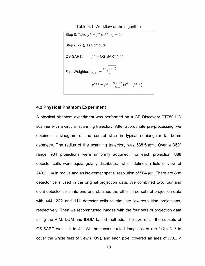
70

Table 4.1. Workflow of the algorithm

Step 0. Take 𝑦1 = 𝑓0 ∈ 𝑅𝑛, 𝑡1 = 1.

Step 𝑘. (𝑘 ≥ 1) Compute

OS-SART: 𝑓𝑘 = OS-SART(𝑦𝑘)

Fast Weighted: 𝑡𝑘+1 =1+�1+4𝑡𝑘

2

2

𝑦𝑘+1 = 𝑓𝑘 + �𝑡𝑘−1𝑡𝑘+1

� �𝑓𝑘 − 𝑓𝑘−1�

4.2 Physical Phantom Experiment

A physical phantom experiment was performed on a GE Discovery CT750 HD

scanner with a circular scanning trajectory. After appropriate pre-processing, we

obtained a sinogram of the central slice in typical equiangular fan-beam

geometry. The radius of the scanning trajectory was 538.5 𝑚𝑚. Over a 360°

range, 984 projections were uniformly acquired. For each projection, 888

detector cells were equiangularly distributed, which defines a field of view of

249.2 𝑚𝑚 in radius and an iso-center spatial resolution of 584 µ𝑚. There are 888

detector cells used in the original projection data. We combined two, four and

eight detector cells into one and obtained the other three sets of projection data

with 444, 222 and 111 detector cells to simulate low-resolution projections,

respectively. Then we reconstructed images with the four sets of projection data

using the AIM, DDM and IDDM based methods. The size of all the subsets of

OS-SART was set to 41. All the reconstructed image sizes are 512 × 512 to

cover the whole field of view (FOV), and each pixel covered an area of 973.3 ×

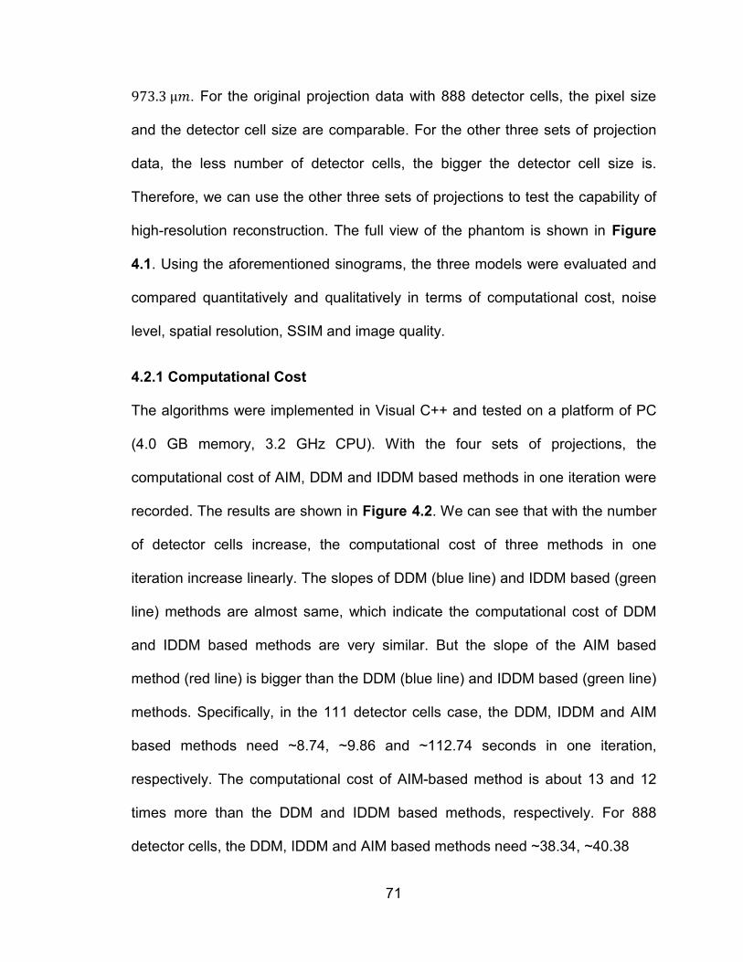
71

973.3 µ𝑚. For the original projection data with 888 detector cells, the pixel size

and the detector cell size are comparable. For the other three sets of projection

data, the less number of detector cells, the bigger the detector cell size is.

Therefore, we can use the other three sets of projections to test the capability of

high-resolution reconstruction. The full view of the phantom is shown in Figure

4.1. Using the aforementioned sinograms, the three models were evaluated and

compared quantitatively and qualitatively in terms of computational cost, noise

level, spatial resolution, SSIM and image quality.

4.2.1 Computational Cost

The algorithms were implemented in Visual C++ and tested on a platform of PC

(4.0 GB memory, 3.2 GHz CPU). With the four sets of projections, the

computational cost of AIM, DDM and IDDM based methods in one iteration were

recorded. The results are shown in Figure 4.2. We can see that with the number

of detector cells increase, the computational cost of three methods in one

iteration increase linearly. The slopes of DDM (blue line) and IDDM based (green

line) methods are almost same, which indicate the computational cost of DDM

and IDDM based methods are very similar. But the slope of the AIM based

method (red line) is bigger than the DDM (blue line) and IDDM based (green line)

methods. Specifically, in the 111 detector cells case, the DDM, IDDM and AIM

based methods need ~8.74, ~9.86 and ~112.74 seconds in one iteration,

respectively. The computational cost of AIM-based method is about 13 and 12

times more than the DDM and IDDM based methods, respectively. For 888

detector cells, the DDM, IDDM and AIM based methods need ~38.34, ~40.38

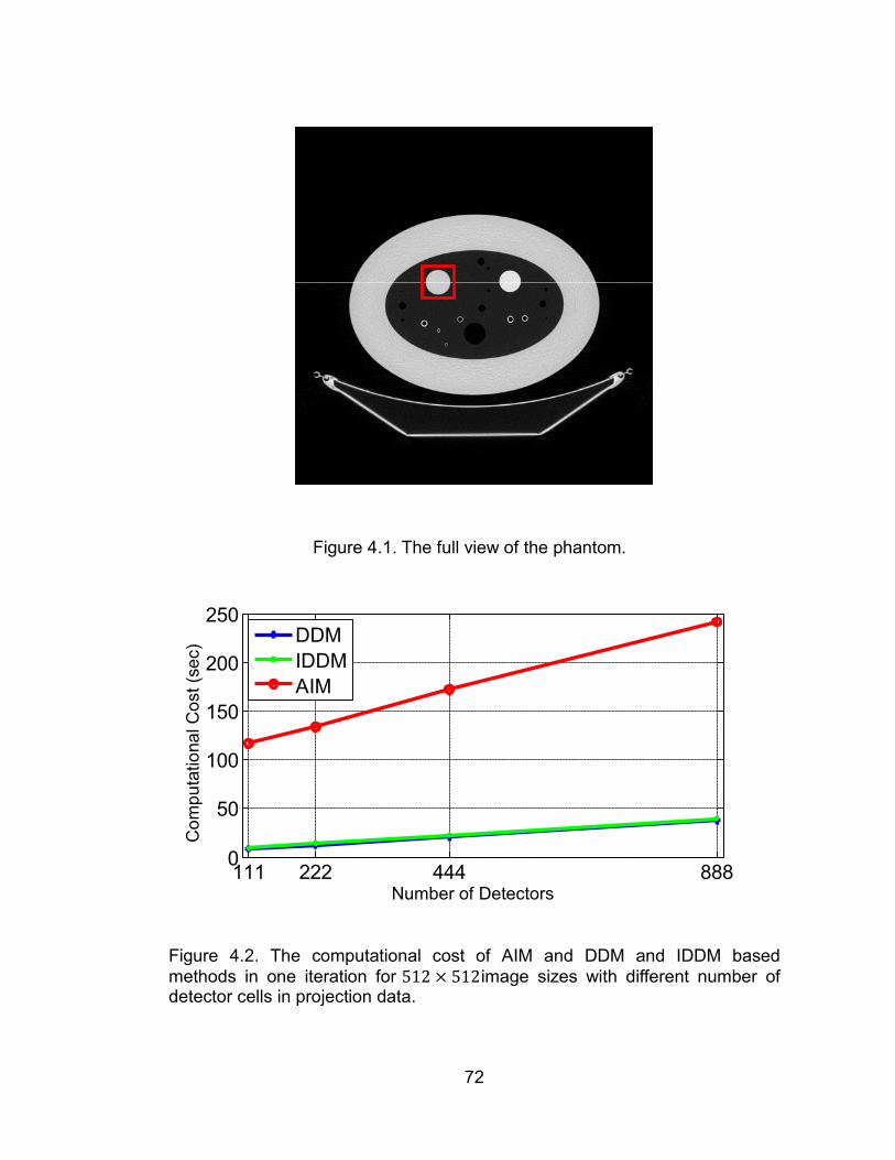
72

111 222 444 8880

50

100

150

200

250

DDMIDDMAIM

Com

puta

tiona

l Cos

t (se

c)

Number of Detectors

Figure 4.2. The computational cost of AIM and DDM and IDDM based methods in one iteration for 512 × 512image sizes with different number of detector cells in projection data.

Figure 4.1. The full view of the phantom.

73

and ~242.34 seconds in one iteration, respectively.

4.2.2 Image Noise

The standard variance of the pixel values within a homogenous region were

computed to measure the image noises using Equation 4.1:

𝜎 = �1𝐵∑ �𝑓𝑗 − 𝑓𝑚�

2𝐵𝑗=1 (4.1)

where 𝐵 is the total number of pixels in the selected flat region, 𝑓𝑚 is the mean of

the region. The experimental results are shown in Figure 4.3. We can see that,

for the case of 888 detector cells, the image noise of three methods are very

similar before 30 iterations, but the IDDM based has a little bit smaller image

noise than the DDM and AIM based methods. After that, the image noises begin

to level off and the DDM and IDDM based methods have the lowest and highest

image noises. Actually, we can get a satisfactory reconstructed image with 20

iterations. We can also see that with the increase of the iteration number, the

image noise of three methods decrease and then increase and level off finally. At

the beginning, the low frequency components are reconstructed and result in

smoother reconstructions. Then, the high frequency components are

reconstructed, and the noise image will be reconstructed from the noise in the

projection data. Therefore, after certain number of iterations (4 iterations), the

noise in the reconstructed images begin to increase and level off finally. For the

cases of 444 and 222 detector cells, the image noise performance is very similar

with the first one. But the image noises begin to level off later than the first one

(not shown in this figure). It is becomes more apparent that the IDDM based

74

method has a smaller image noise before level off. For the case of 111 detector

cells, the image noise decrease to reach to the minimum (3 iterations) and then

increase and reach to the local maximum, and decrease again and reach the

second minimum, and then increase.

For a qualitative comparison, the reconstructed images and profiles along

the white line in Figure 4.1 are shown in Figures 4.4-4.7. For the case of 888

detector cells, as indicated in Figure 4.4, the reconstructed images with 4

(minimum image noise) and 40 iterations are shown in the first and second rows,

respectively. There is no detectable difference between the reconstructed images

in the same row visually. However, we can see that, the three images in the first

row are smoother than the second row. The first row images are mostly

composed by low frequency components and have smaller image noise. On the

other hand, there are more high frequency components in the second row

images, and we can see more details of the phantom. From the magnified region

shown in the first row, we can barely recognize the difference, because the

reconstructed images by three methods with 4 iterations have similar image

noise. From the magnified region in the second row, we can see that the

magnitudes of IDDM based method are a little bit larger than AIM and DDM. The

DDM based method has the smallest magnitudes. However, the difference is not

so obvious. This is because the image noises of three methods begin to level off

at 40 iterations and the IDDM based methods have a little bit larger image noise

(after level off).

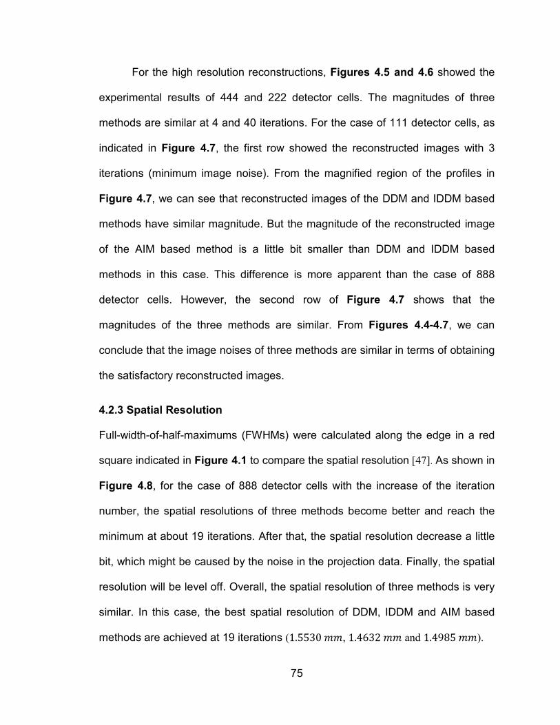
75

For the high resolution reconstructions, Figures 4.5 and 4.6 showed the

experimental results of 444 and 222 detector cells. The magnitudes of three

methods are similar at 4 and 40 iterations. For the case of 111 detector cells, as

indicated in Figure 4.7, the first row showed the reconstructed images with 3

iterations (minimum image noise). From the magnified region of the profiles in

Figure 4.7, we can see that reconstructed images of the DDM and IDDM based

methods have similar magnitude. But the magnitude of the reconstructed image

of the AIM based method is a little bit smaller than DDM and IDDM based

methods in this case. This difference is more apparent than the case of 888

detector cells. However, the second row of Figure 4.7 shows that the

magnitudes of the three methods are similar. From Figures 4.4-4.7, we can

conclude that the image noises of three methods are similar in terms of obtaining

the satisfactory reconstructed images.

4.2.3 Spatial Resolution

Full-width-of-half-maximums (FWHMs) were calculated along the edge in a red

square indicated in Figure 4.1 to compare the spatial resolution [47]. As shown in

Figure 4.8, for the case of 888 detector cells with the increase of the iteration

number, the spatial resolutions of three methods become better and reach the

minimum at about 19 iterations. After that, the spatial resolution decrease a little

bit, which might be caused by the noise in the projection data. Finally, the spatial

resolution will be level off. Overall, the spatial resolution of three methods is very

similar. In this case, the best spatial resolution of DDM, IDDM and AIM based

methods are achieved at 19 iterations (1.5530 𝑚𝑚, 1.4632 𝑚𝑚 and 1.4985 𝑚𝑚).

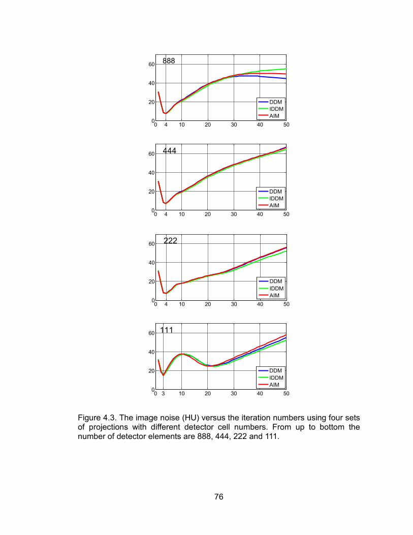
76

0 4 10 20 30 40 500

20

40

60

DDMIDDMAIM

888

0 4 10 20 30 40 500

20

40

60

DDMIDDMAIM

444

0 3 10 20 30 40 500

20

40

60

DDMIDDMAIM

111

0 4 10 20 30 40 500

20

40

60

DDMIDDMAIM

222

Figure 4.3. The image noise (HU) versus the iteration numbers using four sets of projections with different detector cell numbers. From up to bottom the number of detector elements are 888, 444, 222 and 111.

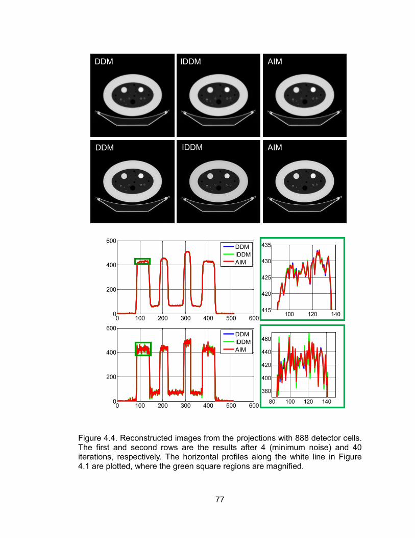
77

DDM AIM IDDM

DDM AIM IDDM

0 100 200 300 400 500 6000

200

400

600

DDMIDDMAIM

0 100 200 300 400 500 6000

200

400

600

DDMIDDMAIM

100 120 140415

420

425

430

435

80 100 120 140

380

400

420

440

460

Figure 4.4. Reconstructed images from the projections with 888 detector cells. The first and second rows are the results after 4 (minimum noise) and 40 iterations, respectively. The horizontal profiles along the white line in Figure 4.1 are plotted, where the green square regions are magnified.

78

DDM AIM

DDM AIM

IDDM

IDDM

80 100 120 140

380

400

420

440

460

100 120 140415

420

425

430

435

0 100 200 300 400 500 6000

200

400

600

DDMIDDMAIM

0 100 200 300 400 500 6000

200

400

600

DDMIDDMAIM

Figure 4.5. Same as Figure 4.4 but reconstructed from the projections with 444 detector cells.

79

DDM AIM

DDM AIM IDDM

IDDM

100 120 140415

420

425

430

435

0 100 200 300 400 500 6000

200

400

600

DDMIDDMAIM

0 100 200 300 400 500 6000

200

400

600

DDMIDDMAIM

80 100 120 140

380

400

420

440

460

Figure 4.6. Same as Figure 4.4 but reconstructed from the projections with 222 detector cells.

80

0 100 200 300 400 500 6000

200

400

600

DDMIDDMAIM

100 120 140415

420

425

430

435

0 100 200 300 400 500 6000

200

400

600

DDMIDDMAIM

80 100 120 140

380

400

420

440

460

DDM AIM

DDM AIM

IDDM

IDDM

Figure 4.7. Same as Figure 4.4 but reconstructed from the projections with 111 detector cells.

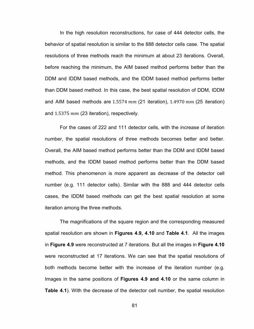
81

In the high resolution reconstructions, for case of 444 detector cells, the

behavior of spatial resolution is similar to the 888 detector cells case. The spatial

resolutions of three methods reach the minimum at about 23 iterations. Overall,

before reaching the minimum, the AIM based method performs better than the

DDM and IDDM based methods, and the IDDM based method performs better

than DDM based method. In this case, the best spatial resolution of DDM, IDDM

and AIM based methods are 1.5574 𝑚𝑚 (21 iteration), 1.4970 𝑚𝑚 (25 iteration)

and 1.5375 𝑚𝑚 (23 iteration), respectively.

For the cases of 222 and 111 detector cells, with the increase of iteration

number, the spatial resolutions of three methods becomes better and better.

Overall, the AIM based method performs better than the DDM and IDDM based

methods, and the IDDM based method performs better than the DDM based

method. This phenomenon is more apparent as decrease of the detector cell

number (e.g. 111 detector cells). Similar with the 888 and 444 detector cells

cases, the IDDM based methods can get the best spatial resolution at some

iteration among the three methods.

The magnifications of the square region and the corresponding measured

spatial resolution are shown in Figures 4.9, 4.10 and Table 4.1. All the images

in Figure 4.9 were reconstructed at 7 iterations. But all the images in Figure 4.10

were reconstructed at 17 iterations. We can see that the spatial resolutions of

both methods become better with the increase of the iteration number (e.g.

Images in the same positions of Figures 4.9 and 4.10 or the same column in

Table 4.1). With the decrease of the detector cell number, the spatial resolution

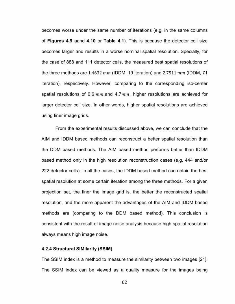
82

becomes worse under the same number of iterations (e.g. in the same columns

of Figures 4.9 aand 4.10 or Table 4.1). This is because the detector cell size

becomes larger and results in a worse nominal spatial resolution. Specially, for

the case of 888 and 111 detector cells, the measured best spatial resolutions of

the three methods are 1.4632 𝑚𝑚 (IDDM, 19 iteration) and 2.7511 𝑚𝑚 (IDDM, 71

iteration), respectively. However, comparing to the corresponding iso-center

spatial resolutions of 0.6 𝑚𝑚 and 4.7𝑚𝑚, higher resolutions are achieved for

larger detector cell size. In other words, higher spatial resolutions are achieved

using finer image grids.

From the experimental results discussed above, we can conclude that the

AIM and IDDM based methods can reconstruct a better spatial resolution than

the DDM based methods. The AIM based method performs better than IDDM

based method only in the high resolution reconstruction cases (e.g. 444 and/or

222 detector cells). In all the cases, the IDDM based method can obtain the best

spatial resolution at some certain iteration among the three methods. For a given

projection set, the finer the image grid is, the better the reconstructed spatial

resolution, and the more apparent the advantages of the AIM and IDDM based

methods are (comparing to the DDM based method). This conclusion is

consistent with the result of image noise analysis because high spatial resolution

always means high image noise.

4.2.4 Structural SIMilarity (SSIM)

The SSIM index is a method to measure the similarity between two images [21].

The SSIM index can be viewed as a quality measure for the images being

83

compared, providing the other image is regarded as of perfect quality. If the

measured image is exactly same with the reference image, the SSIM index will

be equal to 1. The best spatial resolutions are achieved by the DDM, IDDM and

AIM based methods after 19 iterations from the projection data with 888 detector

cells, respectively. The corresponding images are averaged to obtain a reference

image. The SSIM indexes are computed for the same images as Table 4.2. From

Table 4.3 we can conclude that, the AIM-based method is better than the DDM

and IDDM based methods in the 7 iterations. In the 17 iterations, the AIM and

IDDM based methods perform better than DDM based method. As the decrease

of the detector cell number, the image quality becomes worse after the same

number of iterations, which is consistent with Figures 4.9 and 4.10.

4.3 Discussion and Conclusion

In conclusion, we have numerically evaluated the AIM, DDM and IDDM based

methods in an OS-SART framework. The proposed improved distance-driven

model (IDDM) has a computational cost as low as DDM and a spatial resolution

as high as AIM. Because the AIM based method requires higher computation

cost to compute the system matrix 𝑊 analytically, the DDM and IDDM based

methods are faster than the AIM based method. While three methods have

similar image noise performance, the AIM based method has a little bit better

performance in terms of spatial resolution and SSIM especially in the high

resolution reconstruction cases. The IDDM based method can obtain the best

spatial resolution at some certain iteration among the three methods. The

84

proposed IDDM based method is reasonable because it can meet the

requirements of higher spatial resolution with low computational cost.

Table 4.3. SSIM index of DDM, IDDM and AIM based methods

Table 4.2. Measured spatial resolution of DDM, IDDM and AIM based methods

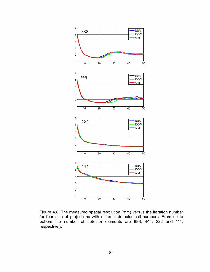
85

10 20 30 40 501

2

3

4

5

6

DDMIDDMAIM

888

10 20 30 40 501

2

3

4

5

6

DDMIDDMAIM

444

10 20 30 40 501

2

3

4

5

6

DDMIDDMAIM

222

10 20 30 40 501

2

3

4

5

6

DDMIDDMAIM

111

Figure 4.8. The measured spatial resolution (mm) versus the iteration number for four sets of projections with different detector cell numbers. From up to bottom the number of detector elements are 888, 444, 222 and 111, respectively.

86

DDM 07 IDDM 07 AIM 07

Figure 4.9. Magnifications of the square region indicated in Figure 4.1. From top to bottom, the detector cell numbers are 888, 444, 222 and 111, respectively. From the first to third columns, the system models are DDM, IDDM and AIM. All the reconstructed images are come from 7 iterations.

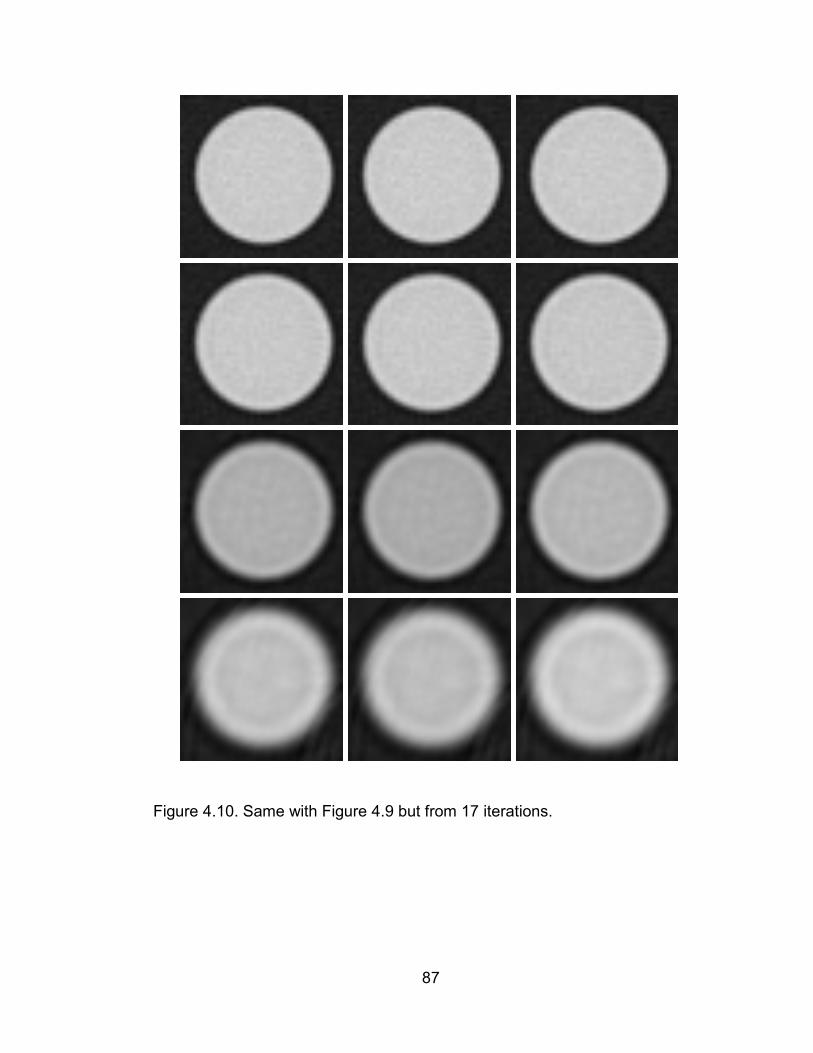
87

Figure 4.10. Same with Figure 4.9 but from 17 iterations.

88

5. Conclusions and Future Work

In this thesis, we proposed an IDDM which the computational cost is as low as

DDM and the accuracy is comparable with AIM. The goal of this thesis was to

compare the performance of different system models (PDM, RDM, AIM, DDM

and IDDM) in the iterative CT image reconstruction. We achieved this goal in

several stages. First, we illustrate the computation of the weighting coefficient in

each model assuming a typical fan beam geometry (Section 2.2). Second, we

theoretically analyzed the performance of different system models assuming a

parallel beam geometry assuming the detector element size is larger,

comparable and smaller than the image pixel size (Section 2.3). The results can

always be extended to the fan beam geometry and even the cone beam

geometry. Then, we demonstrated the analysis by some experiments (such as

pixel support) employ the projection and backprojection operations separately.

The results shows that the AIM, DDM and IDDM based methods are superior

compare to the PDM and RDM models based methods. The AIM based method

is superior compare to DDM and IDDM based methods in terms of the high

resolution reconstruction but at the cost of higher computational cost. The

accuracy of IDDM based method is between the DDM and AIM based methods

but with a similar low computational cost with DDM based method. Finally, in

order to further compare the performance of AIM, DDM and IDDM based

methods in a more practical way, we designed a physical phantom experiment

and the results are consistent with the analysis in Section 2.

89

One of the most important factors that limit the clinical application of the

iterative reconstruction algorithm is the slow reconstruction speed. In the future,

we will study the acceleration of different models such as AIM, DDM and IDDM.

For example, we can employ some parallelization techniques and GPU-based

methods to accelerate the projection and backprojection processes. In sum, this

thesis can be the basic work before the acceleration study and will have a direct

impact of the development of the fast and accurate iterative CT image

reconstruction algorithm.

90

References

1. Mahesh, M., The AAPM/RSNA Physics Tutorial for Residents.

RadioGraphics, 2002. 22: p. 949-962.

2. Burnham, C.A. and G.L. Brownell, A Multi-Crystal Positron Camera.

Nuclear Science, IEEE Transactions on, 1972. 19(3): p. 201-205.

3. Ter-Pogossian, M.M., et al., A positron-emission transaxial tomograph for

nuclear imaging (PETT). Radiology, 1975. 114(1): p. 89-98.

4. Phelps, M.E., et al., Application of annihilation coincidence detection to

transaxial reconstruction tomography. J Nucl Med, 1975. 16(3): p. 210-24.

5. Andersen, A.H., Algebraic reconstruction in CT from limited views. Medical

Imaging, IEEE Transactions on, 1989. 8(1): p. 50-55.

6. Kuhl, D.E. and R.Q. Edwards, Image Separation Radioisotope Scanning.

Radiology, 1963. 80: p. 653-662.

7. Jasczak, R.J., Tomographic radiopharmaceutical imaging. Proceedings of

the IEEE, 1988. 76(9): p. 1079-1094.

8. Neumann, D.R., N.A. Obuchowski, and F.P. Difilippo, Preoperative

123I/99mTc-sestamibi subtraction SPECT and SPECT/CT in primary

hyperparathyroidism. J Nucl Med, 2008. 49(12): p. 2012-7.

9. Sheil, W.C., Magnetic Resonance Imaging (MRI Scan). MedicineNet.com.

Retrieved 08 Feb. 2013.

91

10. Herman, G.T. and A. Lent, Iterative reconstruction algorithms. Computers

in Biology and Medicine, 1976. 6(4): p. 273-294.

11. Hendee, W.R. and C.J. Morgan, Magnetic Resonance Imaging Part I --

Physical Principles. Western Journal of Medicine, 1984. 141(4): p. 491-500.

12. Mohan, R., A. Singh, and S. Gundappa, Three-dimensional imaging in

periodontal diagnosis - Utilization of cone beam computed tomography. Journal

of Indian Society of Periodontology, 2011. 15(1): p. 11-17.

13. Kak, A.C. and M. Slaney, Principles of Computerized Tomographic

Imaging (New York: IEEE Press). 1999.

14. De Man, B. and S. Basu, Distance-driven projection and backprojection in

three dimensions. Phys Med Biol, 2004. 49(11): p. 2463-75.

15. Herman, G.T., Image Reconstruction from projections (Orlando:

Academic). 1980.

16. Peters, T.M., Algorithms for Fast Back- and Re-Projection in Computed

Tomography. IEEE transactions on nuclear science, 1981. 28(4): p. 3641-3647.

17. Zhuang, W., S. Gopal, and T.J. Hebert. Numerical evaluation of methods

for computing tomographic projections. 1994.

18. De Man, B. and S. Basu, Distance-driven projection and backprojection.

IEEE Nuclear Science Symp. Medical Imaging Conf. (Norfolk), 2002.

19. De Man, B. and S. Basu, 3D distance-driven projection and backprojection.

Proc. 7th Int. Conf. on Fully 3D Reconstruction in Radiology and Nuclear

Medicine (Saint Malo), 2003.

92

20. Yu, H. and G. Wang, Finite detector based projection model for high

spatial resolution. Journal of X-ray science and technology, 2012. 20(2): p. 229-

38.

21. Zhou, W., et al., Image quality assessment: from error visibility to

structural similarity. Image Processing, IEEE Transactions on, 2004. 13(4): p.

600-612.

22. Zeng, G. and G. Gullberg, A ray-driven backprojector for backprojection

filtering and filtered backprojection algorithms. IEEE Nuclear Science Symp.

Medical Imaging Conf. (San Francisco), 1993: p. 1199-201.

23. L.Westover, Footprint Evaluation for Volume Rendering. Computer

Graphics, Proc. SIGGRAPH, 1990: p. 367-376.

24. Herman, G.T., Image reconstruction from projections. Academic Press,

1980.

25. Zhuang, W., G.S. S., and T.J. Hebert. Numerical evaluation of methods for

computing tomographic projections. 1994.

26. Siddon, R.L., Fast calculation of the exact radiological path length for a

three-dimensional CT array. Med. Phys., 1985. 12(2): p. 252-255.

27. Zeng, G.L. and G.T. Gullberg, A Ray-driven Backprojector For

Backprojection Filtering And Filtered Backprojection Algorithms. Nuclear Science

Symposium and Medical Imaging Conference, 1993: p. 1199-1201.

28. Joseph, P.M., An Improved Algorithm for Reprojecting Rays through Pixel

Images. Medical Imaging, IEEE Transactions on, 1982. 1(3): p. 192-196.

93

29. Gordon, R., R. Bender, and G.T. Herman, Algebraic Reconstruction

Techniques (ART) for three-dimensional electron microscopy and X-ray

photography. Journal of Theoretical Biology, 1970. 29(3): p. 471-481.

30. Censor, Y., P.B. Eggermont, and D. Gordon, Strong underrelaxation in

Kaczmarz's method for inconsistent systems. Numerische Mathematik, 1983.

41(1): p. 83-92.

31. Andersen, A.H. and A.C. Kak, Simultaneous algebraic reconstruction

technique (SART): a superior implementation of the art algorithm. Ultrason

Imaging, 1984. 6(1): p. 81-94.

32. Ming, J. and W. Ge, Convergence of the simultaneous algebraic

reconstruction technique (SART). Image Processing, IEEE Transactions on,

2003. 12(8): p. 957-961.

33. Rockmore, A.J. and A. Macovski, A Maximum Likelihood Approach to

Emission Image Reconstruction from Projections. Nuclear Science, IEEE

Transactions on, 1976. 23(4): p. 1428-1432.

34. Shepp, L.A. and Y. Vardi, MAXIMUM LIKELIHOOD RECONSTRUCTION

FOR EMISSION TOMOGRAPHY. Journal of computer assisted tomography,

1983. 7(3): p. 571.

35. Lange, K. and R. Carson, EM reconstruction algorithms for emission and

transmission tomography. Journal of computer assisted tomography, 1984. 8(2):

p. 306-16.

94

36. Lucy, L.B., An iterative technique for the rectification of observed

distribution. The Smithsonian/NASA Astrophysics Data System, 1974. 79: p. 745-

754.

37. William Hadley, R., Bayesian-Based Iterative Method of Image

Restoration. Journal of the Optical Society of America (1930), 1972. 62(1): p. 55-

59.

38. Sotthivirat, S. and J.A. Fessler, Relaxed ordered-subset algorithm for

penalized-likelihood image restoration. J Opt Soc Am A Opt Image Sci Vis, 2003.

20(3): p. 439-49.

39. Hudson, H.M. and R.S. Larkin, Accelerated image reconstruction using

ordered subsets of projection data. Medical Imaging, IEEE Transactions on, 1994.

13(4): p. 601-609.

40. Kamphuis, C. and F.J. Beekman, Accelerated iterative transmission CT

reconstruction using an ordered subsets convex algorithm. Medical Imaging,

IEEE Transactions on, 1998. 17(6): p. 1101-1105.

41. Erdogan, H. and J.A. Fessler, Ordered subsets algorithms for

transmission tomography. Phys. Med. Biol., 1999. 44(11).

42. Byrne, C.L., Block-iterative methods for image reconstruction from

projections. Image Processing, IEEE Transactions on, 1996. 5(5): p. 792-794.

43. Byrne, C.L., Accelerating the EMML algorithm and related iterative

algorithms by rescaled block-iterative methods. Image Processing, IEEE

Transactions on, 1998. 7(1): p. 100-109.

95

44. Censor, Y. and T. Elfving, Block-Iterative Algorithms with Diagonally

Scaled Oblique Projections for the Linear Feasibility Problem. SIAM Journal on

Matrix Analysis and Applications, 2002. 24(1): p. 40-19.

45. Wang, G. and M. Jiang, Ordered-subset simultaneous algebraic

reconstruction techniques (OS-SART). Journal of X-ray science and technology,

2004. 12(3): p. 169-177.

46. Beck, A. and M. Teboulle, A Fast Iterative Shrinkage-Thresholding

Algorithm for Linear Inverse Problems. SIAM Journal on Imaging Sciences, 2009.

2(1): p. 20.

47. Schlueter, F.J., et al., Longitudinal image deblurring in spiral CT.

Radiology, 1994. 193(2): p. 413-8.

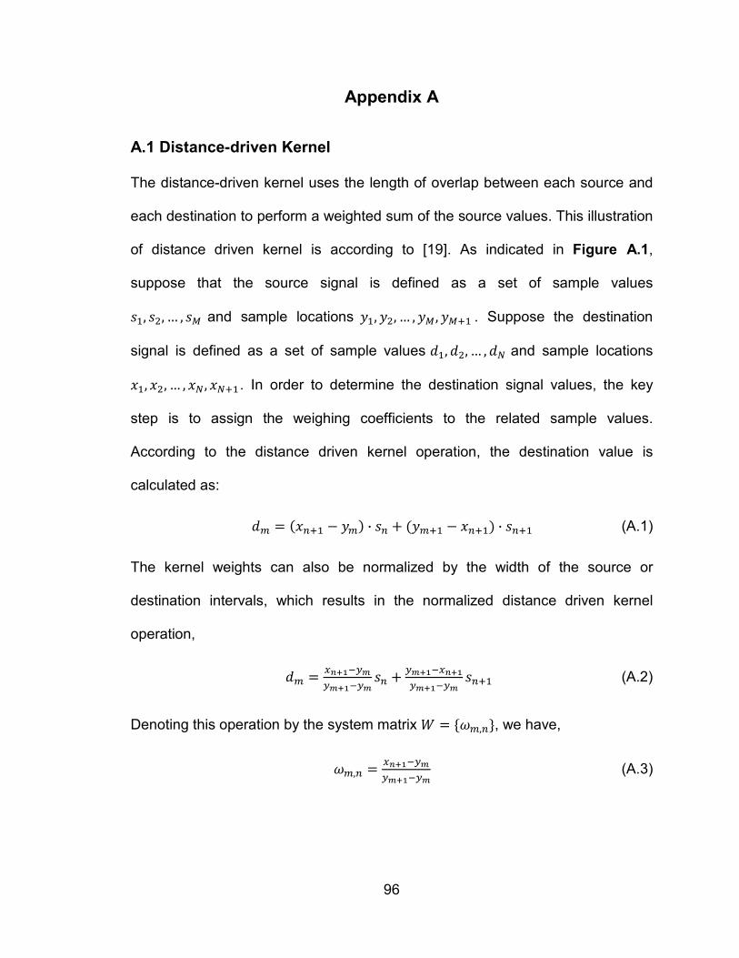
96

Appendix A

A.1 Distance-driven Kernel

The distance-driven kernel uses the length of overlap between each source and

each destination to perform a weighted sum of the source values. This illustration

of distance driven kernel is according to [19]. As indicated in Figure A.1,

suppose that the source signal is defined as a set of sample values

𝑠1, 𝑠2, … , 𝑠𝑀 and sample locations 𝑦1,𝑦2, … ,𝑦𝑀 ,𝑦𝑀+1 . Suppose the destination

signal is defined as a set of sample values 𝑑1,𝑑2, … ,𝑑𝑁 and sample locations

𝑥1, 𝑥2, … , 𝑥𝑁 , 𝑥𝑁+1. In order to determine the destination signal values, the key

step is to assign the weighing coefficients to the related sample values.

According to the distance driven kernel operation, the destination value is

calculated as:

𝑑𝑚 = (𝑥𝑛+1 − 𝑦𝑚) ∙ 𝑠𝑛 + (𝑦𝑚+1 − 𝑥𝑛+1) ∙ 𝑠𝑛+1 (A.1)

The kernel weights can also be normalized by the width of the source or

destination intervals, which results in the normalized distance driven kernel

operation,

𝑑𝑚 = 𝑥𝑛+1−𝑦𝑚𝑦𝑚+1−𝑦𝑚

𝑠𝑛 + 𝑦𝑚+1−𝑥𝑛+1𝑦𝑚+1−𝑦𝑚

𝑠𝑛+1 (A.2)

Denoting this operation by the system matrix 𝑊 = {𝜔𝑚,𝑛}, we have,

𝜔𝑚,𝑛 = 𝑥𝑛+1−𝑦𝑚𝑦𝑚+1−𝑦𝑚

(A.3)

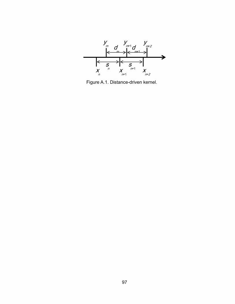
97

ym y

m+1 y

m+2

xn+1

xn x

n+2

dm d

m+1

sn s

n+1

Figure A.1. Distance-driven kernel.

98

Curriculum Vitae

Chuang Miao was born in Jinlin province, China. He attended high school there

and received a high school diploma from Shiyan High School in 2006. He

subsequently attended the Jilin University, China, where he completed Bachelor

of Engineering degree in Electrical Engineering in 2010. He subsequently

attended the VT-WFU School of Biomedical Engineering and Sciences, Wake

Forest University, USA in 2011. He completed Master of Sciences degree in this

university in May 2013. He is continuing his research toward a doctorate.