02/11/2015

Tanvi_14ME14_Review4

Comparative Study of Graph Partitioning Algorithms

Graph Partitioning is an important problem in area of VLSI design.

Partitioning is used to find strongly connected components that can be placed together in order to minimize the layout area and propagation delay.

Introduction

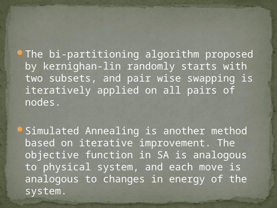
The bi-partitioning algorithm proposed by kernighan-lin randomly starts with two subsets, and pair wise swapping is iteratively applied on all pairs of nodes.

Simulated Annealing is another method based on iterative improvement. The objective function in SA is analogous to physical system, and each move is analogous to changes in energy of the system.

The simulated annealing (SA) algorithm is a widely used iterative technique for solving general optimization problems. It is an adaptive heuristic and belongs to the class of non-deterministic algorithms.

Locates a good approximation to the global optimum in a large search space.

Simulated Annealing

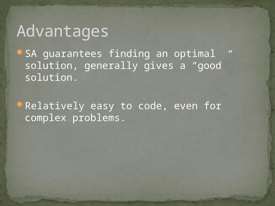
SA guarantees finding an optimal solution, generally gives a “good” solution.

Relatively easy to code, even for complex problems.

Advantages

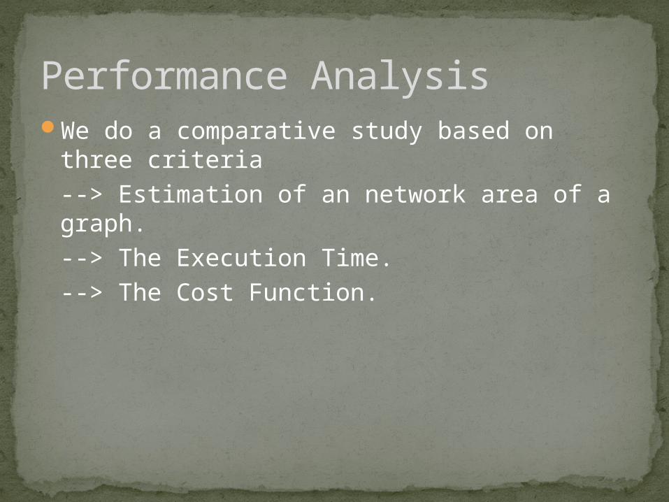
We do a comparative study based on three criteria--> Estimation of an network area of a graph.

--> The Execution Time.--> The Cost Function.

Performance Analysis

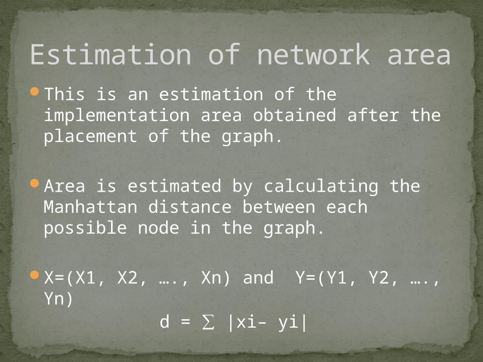
This is an estimation of the implementation area obtained after the placement of the graph.

Area is estimated by calculating the Manhattan distance between each possible node in the graph.

X=(X1, X2, …., Xn) and Y=(Y1, Y2, …., Yn)d = ∑ |xi– yi|

Estimation of network area

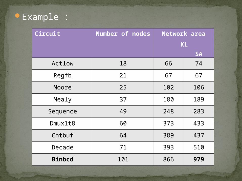
Example :Circuit Number of

nodesNetwork area

KL SA

Actlow 18 66 74

Regfb 21 67 67

Moore 25 102 106

Mealy 37 180 189

Sequence 49 248 283

Dmux1t8 60 373 433

Cntbuf 64 389 437

Decade 71 393 510

Binbcd 101 866 979

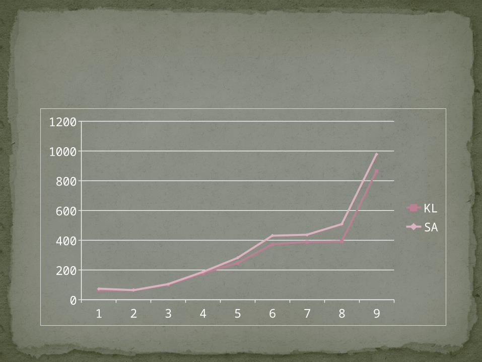
1 2 3 4 5 6 7 8 90

200

400

600

800

1000

1200

KLSA

For a small number of nodes, the difference between result is almost negligible, but when the number of nodes increase, the difference becomes significant.

The result suggest that the solution obtained by KL algorithm are better then by SA algorithm.

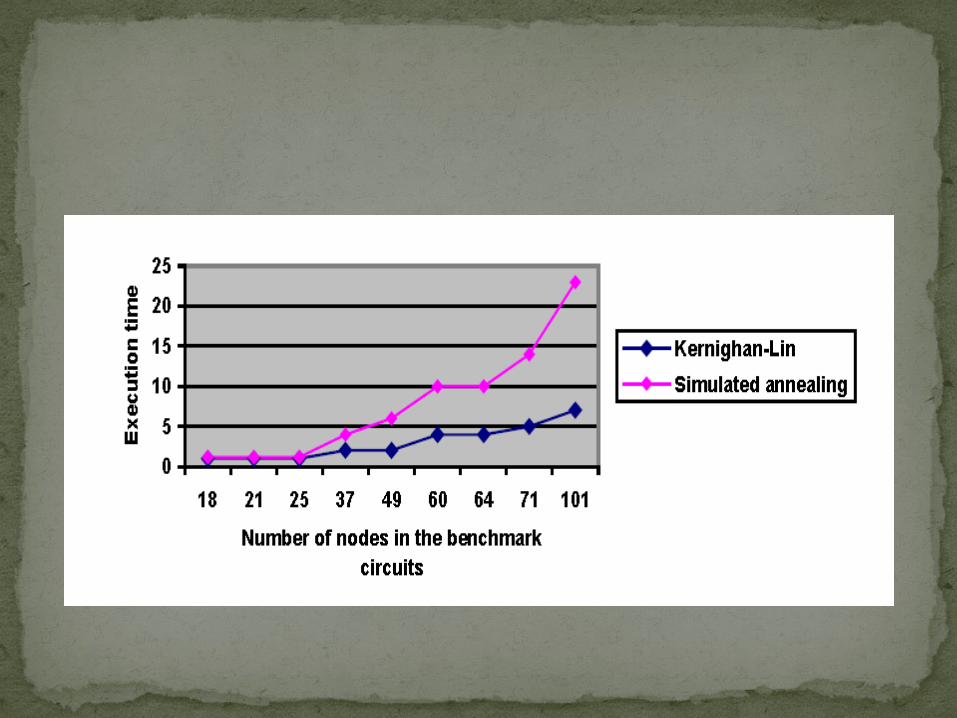
For a small number of nodes, there are no significant differences between the results of two algorithms. But for higher number of nodes, the execution time grows for the SA algorithm

The Execution Time

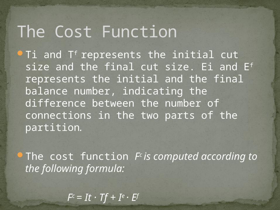
Ti and Tf represents the initial cut size and the final cut size. Ei and Ef represents the initial and the final balance number, indicating the difference between the number of connections in the two parts of the partition.

The cost function Fc is computed according to the following formula:

Fc = It · Tf + Ie · Ef

The Cost Function

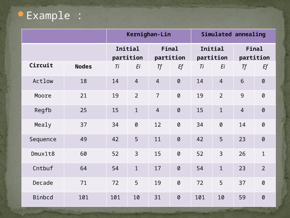
Example :Kernighan-Lin Simulated annealing

Initial partition Final partition Initial partition Final partition

Circuit Nodes Ti Ei Tf Ef Ti Ei Tf Ef

Actlow 18 14 4 4 0 14 4 6 0

Moore 21 19 2 7 0 19 2 9 0

Regfb 25 15 1 4 0 15 1 4 0

Mealy 37 34 0 12 0 34 0 14 0

Sequence 49 42 5 11 0 42 5 23 0

Dmux1t8 60 52 3 15 0 52 3 26 1

Cntbuf 64 54 1 17 0 54 1 23 2

Decade 71 72 5 19 0 72 5 37 0

Binbcd 101 101 10 31 0 101 10 59 0

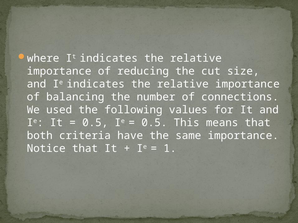
where It indicates the relative importance of reducing the cut size, and Ie indicates the relative importance of balancing the number of connections. We used the following values for It and Ie: It = 0.5, Ie = 0.5. This means that both criteria have the same importance. Notice that It + Ie = 1.

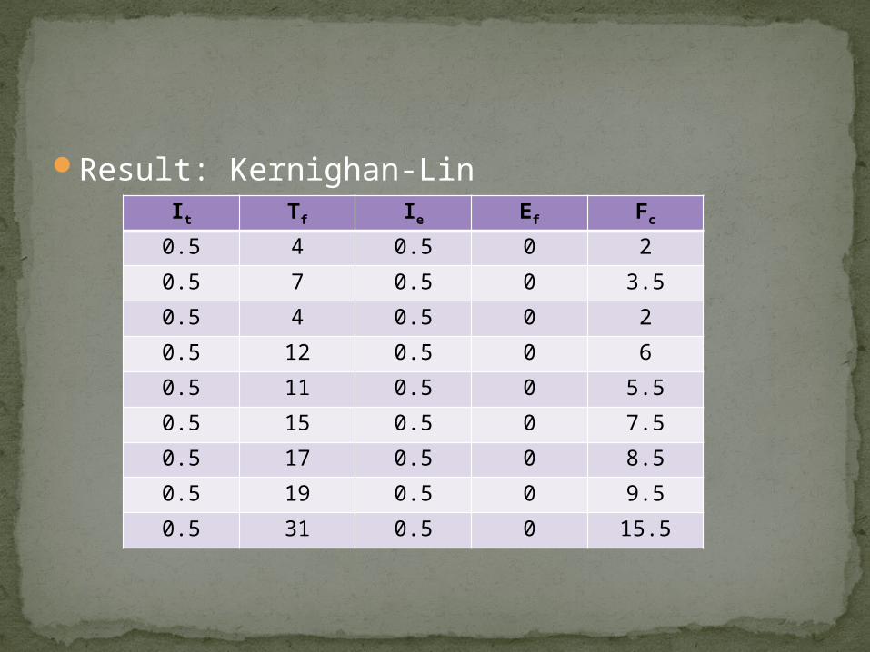
Result: Kernighan-LinIt Tf Ie Ef Fc

0.5 4 0.5 0 2

0.5 7 0.5 0 3.5

0.5 4 0.5 0 2

0.5 12 0.5 0 6

0.5 11 0.5 0 5.5

0.5 15 0.5 0 7.5

0.5 17 0.5 0 8.5

0.5 19 0.5 0 9.5

0.5 31 0.5 0 15.5

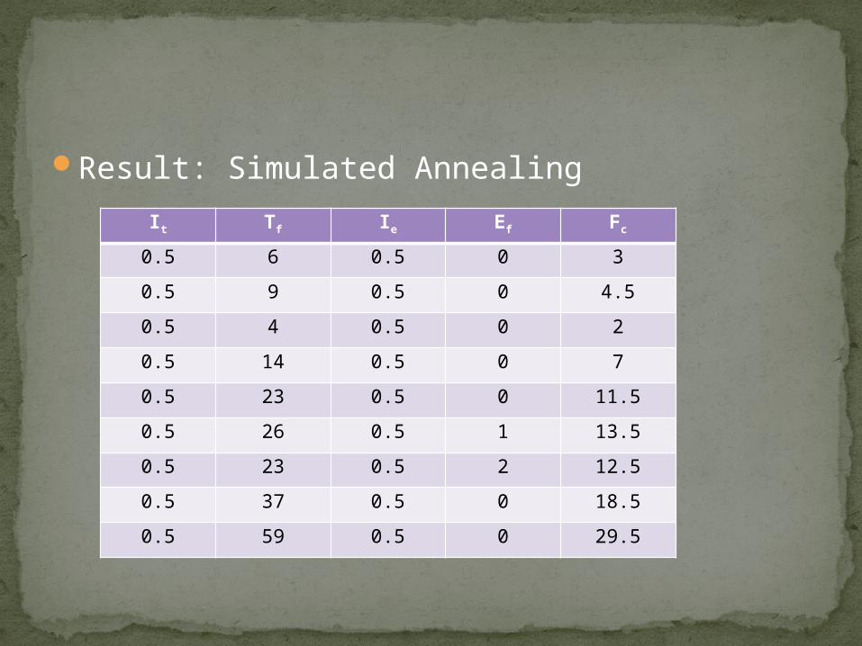
Result: Simulated Annealing It Tf Ie Ef Fc

0.5 6 0.5 0 3

0.5 9 0.5 0 4.5

0.5 4 0.5 0 2

0.5 14 0.5 0 7

0.5 23 0.5 0 11.5

0.5 26 0.5 1 13.5

0.5 23 0.5 2 12.5

0.5 37 0.5 0 18.5

0.5 59 0.5 0 29.5

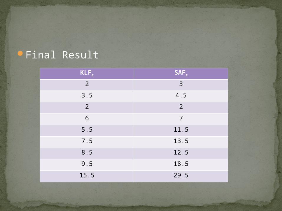
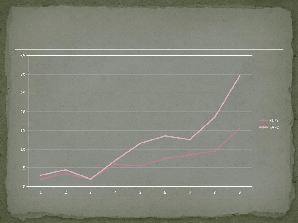
Final Result KLFc SAFc

2 3

3.5 4.5

2 2

6 7

5.5 11.5

7.5 13.5

8.5 12.5

9.5 18.5

15.5 29.5

1 2 3 4 5 6 7 8 90

5

10

15

20

25

30

35

KLFcSAFc

The results show that the KL algorithm produces the best results when we consider the execution time and the cost function. From the point of view of the estimated network area, the differences are not significant.

Conclusion

Comparative Study of Circuit Partitioning Algorithms by Zoltan Baruch, Octavian Creţ, Kalman Pusztai .

References: