comparing agricultural total factor productivity between ... · comparing agricultural total factor...

38 NUMB E R 29 , FALL 2015

Comparing Agricultural Total Factor Productivity between Australia, Canada, and the United States, 1961-2006

Yu ShengAustralian Department of Agriculture

Eldon BallU.S. Department of Agriculture

Katerina NossalInternational Trade Centre1

ABSTRACT

This article provides a comparison of levels and growth of agricultural total factor

productivity between Australia, Canada, and the United States for the 1961–2006 period. A

production account for agriculture that is consistent across the three countries is

constructed to estimate output, input and total factor productivity, and a dynamic panel

regression is used to link the productivity estimates to potential determinants. We show that

investment in public research and development and infrastructure plays an important role in

explaining differences in productivity levels between countries. The findings provide useful

insights into how public policy could be used to sustain agricultural productivity growth.

GLOBAL AGRICULTURAL OUTPUT HAS more

than tripled over the past half century, driven by

new technologies and increased input use. This

output growth has helped to satisfy increasing

demand for food and fibre as population and

income per capita have increased, and has

thereby stabilized global food prices. Agricul-

tural productivity growth has contributed signif-

icantly to these gains (Fuglie and Wang, 2012).

One of the most important drivers of agricul-

tural productivity growth is technological

progress. This progress has followed two dis-

tinct paths in developed countries, depending

on the initial endowment of resources. Those

possessing relatively abundant capital and land,

for example Australia, Canada and the United

States, have been lead adopters of capital-inten-

sive technologies such as reduced-till cropping,

yield mapping and mechanised mustering, and

thus have achieved high levels of output per

worker. In contrast, land-scarce, labour-rich

developed economies such as Japan, South

Korea and Taiwan have adopted labour-inten-

sive technologies such as green-housing and

1 Yu Sheng is a senior economist of Agricultural and Resource Economics and Sciences (ABARES) at the Austra-

lian Department of Agriculture and Water Resources; Eldon V. Ball is a Senior Economist with the Economic

Research Service, the US Department of Agriculture, and Instituto de Economia, Universidad Carlos III de

Madrid; Katarina Nossal is an independent consultant and a former economist of Agricultural and Resource

Economics and Sciences (ABARES) at the Australian Department of Agriculture and Water Resources. The

authors thank two anonymous referees for comments and all remaining errors belong to the authors. Emails:

[email protected]; [email protected]; [email protected]

INT E R N A T I ON A L PRO DU C T I V I T Y MON I T OR 39

vertical farming technologies, and thus have

achieved high yields per unit of land (Fuglie,

Wang and Ball, 2012).

However, recent evidence suggests that agri-

cultural productivity growth is either stagnant

or slowing in many countries (Alston, Beddow

and Pardey, 2010; World Bank, 2007; Sheng,

Mullen and Zhao, 2011). This is particularly the

case in countries such as Australia and Canada

that have historically relied on the adoption of

capital-intensive technologies to drive produc-

tivity growth, where the inelastic supply of nat-

ural resources (i.e. land) decreases the marginal

benefits obtained from adopting the embodied

technology. In turn, this creates concern about

the sustainability of capital-intensive technolog-

ical progress as a source of ongoing productivity

growth, compared with labour-intensive tech-

nological progress. These concerns are height-

ened by decreasing marginal returns to capital

and t igh tening agr i cu l tura l l and supply

throughout the world.

To gather more empirical evidence on this

issue, this article calculates and compares total

factor productivity (TFP) levels and growth rates

between Australia, Canada and the United States

for the 1961–2006 period. Comparing output,

input and productivity across countries requires

data on relative output and input prices, based on

purchasing power parity (PPP) estimates. We

obtain these relative prices by combining output

and input prices with their quantities in each

country. In the estimation process, the Törnqvist

index with the Caves-Christensen-Diewert for-

mula for transitivity is employed. Productivity

levels in each country are defined as the ratio of

real output to real input, which in turn are con-

structed as their values divided by corresponding

prices. Finally, we use a dynamic panel regression

analysis to link these TFP measures to potential

determinants in the three countries.

This article builds on previous research (for

example, Ball et al., 2001 and 2010) by con-

structing a consistent production account with

which to compile price and quantity data for

agricultural outputs and inputs in Australia,

Canada, and the United States. In addition, the

accounting identity (whereby total output value

equals total input value) is used to derive unob-

served returns to labour, enforcing the assump-

tion of constant returns to scale. Finally, a

quality adjustment has been applied to land and

certain intermediate inputs to eliminate the

undesirable impact of embodied technological

progress when estimating TFP.

The article is organized into five sections.

Section 1 provides a review of methods and data

used in cross-country comparisons of agricul-

tural productivity. Section 2 develops the data

base for each country and describes the method

used to develop comparable productivity esti-

mates. Section 3 documents data sources for

Australia, Canada, and the United States. Sec-

tion 4 presents the results and compares agricul-

tural productivity and its drivers between

Australia, Canada, and the United States. Sec-

tion 5 concludes.

Cross-Country TFP Comparison

in Agriculture: A Literature

ReviewWhile many studies have used index number

methods to estimate agricultural TFP in individ-

ual countries (Fuglie, Wang and Ball, 2012),

international comparisons remain challenging.

Obtaining data remains the most problematic

issue, with some economists warning of ‘insur-

mountable data constraints’ in producing detailed

commodity datasets for the agriculture industry

in different countries (Craig, Pardey and Rose-

boom, 1997). Where established datasets are

available, differences in the treatment of variables

limits the comparability of input and output data

(Capalbo, Ball and Denny, 1990).

Given these limitations, most cross-country

comparisons have drawn on data from the

40 NUMB E R 29 , FALL 2015

United Nations Food and Agriculture Organi-

zation (FAO). Although it lacks price informa-

tion and does not cover all inputs, the FAO

dataset covers many countries over a long time

period. For example, Craig, Pardey and Rose-

boom (1994 and 1997) estimated agricultural

land and labour productivity for 98 countries

between 1961 and 1990 and found that input

mix, input quality and public infrastructure were

significant factors explaining agricultural pro-

ductivity growth differences between countries.

While such partial productivity measures are

likely to overstate overall efficiency improve-

ments (because they do not account for changes

in the use of capital and intermediate inputs),

they nonetheless provide some indication of fac-

tor-saving technical change (Fuglie, 2010).

Coelli and Rao (2005) used FAO data to com-

pare agricultural TFP for 93 countries between

1980 and 2000 using a Malmquist index and data

envelopment analysis (DEA). The Malmquist

index method allows inputs and outputs to be

aggregated through a distance function, without

the need for price data. The results show that

agricultural TFP growth was strong across all

countries before 2000, with some evidence of

catch-up between low and high performing

countries. Ludena et al. (2007) also used the

Malmquist index method to estimate TFP

growth for subsectors of the agriculture industry

(crops and ruminant and non-ruminant live-

stock) for 116 countries between 1961 and 2006.

The study found that TFP growth in developing

and developed countries was converging for

crop and non-ruminant livestock production

activities, and diverging in the ruminant live-

stock sector.

While the Malmquist index method has some

advantages (for example, no price information is

needed for TFP estimation), it also has disad-

vantages. In particular, it is sensitive to the set of

countries compared, and the number of vari-

ables in the model (Lusigi and Thirtle, 1997).

Without a large cross-section of countries, TFP

estimates are likely to suffer from measurement

errors. Also, estimates from Malmquist index

numbers often seem implausible (Coelli and

Rao, 2005; Headey, Alauddin and Rao, 2010),

possibly because of the unrealistic implicit

shadow prices derived for aggregation (Coelli

and Rao, 2005).

For these reasons, wherever reliable price data

are available, ‘superlative’ index methods are

preferred. Superlative index number methods

are widely adopted by national statistical agen-

cies and are recommended by the OECD (2001)

for productivity statistics.

Fuglie (2010) used a Törnqvist index to esti-

mate and compare agricultural TFP growth for

171 countries. While FAO data were used, and

were augmented using a fixed set of average glo-

bal prices from Rao, Maddison and Lee (2002)

for revenue shares, and using input elasticities

from country-level case studies for cost shares.

Fuglie (2010) found that global agricultural

TFP growth had accelerated in recent decades,

particularly among developing countries such as

China and Brazil. This contrasts with recent

estimates of yield and labour productivity which

indicate a global slowdown (Alston, Beddow and

Pardey, 2010).

After considering various approaches for

performing inter-region comparisons of agri-

cultural prices, quantities and productivity,

Bal l et al . (1997) ident i f ied two sui t ab le

options: the Fisher index with an Eltetö-

Köves-Szulc formula (Eltetö and Köves 1964;

Szulc 1964) and the Törnqvist index with the

Caves-Christensen-Diewert formula (Caves,

Christensen and Diewert, 1982). Ball et al.

(2001, 2010) conducted empirical studies to

examine these approaches. To address the data

challenges facing international comparisons

of agricultural productivity, Ball et al. (2001,

2010) developed an internationally consistent

production account system for collecting agri-


cultural input and output data from individual

countries.

Ball et al. (2001) compared agricultural TFP

between the United States and nine European

Union countries. Using 1990 as the base year,

Ball et al. (2001) derived bilateral Fisher price

indexes adjusted by purchasing power parity and

then by the Eltetö-Köves-Szulc (EKS) formula

(for transitivity). Indirect quantity indexes of out-

puts (inputs) were then estimated as total output

(input) value divided by the corresponding price

index. The results showed that agricultural pro-

ductivity converged between the United States

and the nine European Union countries between

1973 and 1993. Accordingly, most of the observed

disparity in output levels between these countries

is caused by differences in input use.

Ball et al . (2010) further developed the

method for comparing TFP across countries by

applying Törnqvist price indexes and the Caves-

Christensen-Diewert formula (to impose transi-

tivity across countries). These studies compared

competitiveness between the United States and

eleven European Union countries over the

period 1973 to 2002. Ball et al. (2010) found that

the apparent catch-up of the European Union

countries was reversed after the mid-1990s, and

significantly weakened the competitiveness of

European Union agriculture relative to that of

the United States.

Using the method advanced by Ball et al. (2010),

this article uses production account data for agri-

culture in Australia, Canada, and the United States

to compare agricultural TFP between countries

and identify its potential drivers.

Measuring Output, Input

and TFP in AgricultureIn this section, we briefly discuss the index

number method used for multilateral compari-

son of agricultural productivity levels. When

using this method, the TFP index is defined as

the ratio of the index of real output to real input,

which in turn are obtained from the nominal

values of output and input by the corresponding

price indexes. The construction of the output

and input price indexes takes into account prices

and quantities of the individual components in

each country, and is adjusted for cross-country

comparability. To identify its underlying drivers,

measures of TFP are then regressed against fac-

tors such as climate conditions, public R&D

knowledge stock, and infrastructure.

Index Method for TFP Estimates

Theoretically, TFP is measured as real output,

, divided by real input, , and its growth is

measured as the difference between output and-

input growth rates (estimated using logarithmic

differentials to time t).

(1)

(2)

where includes land, capital, labour and

intermediate inputs.

Both direct and indirect methods can be used

to derive real output and input. In practice, an

indirect approach is usually preferred, whereby

real output and input quantities are measured as

the gross value of outputs or inputs divided by a

corresponding price index, since value data for

most outputs and inputs are more readily avail-

able than quantity data. Assuming perfect com-

petition and a linearly homogenous production

function, direct and indirect quantity estimates

are equivalent when using a superlative index

that satisfies the factor reversal test (Diewert,

1992). In this sense, the estimation of real out-

put, real input and productivity is converted into

the estimation of output and input relative

prices.

For each country, output and input price

indexes can be obtained by using a Törnqvist

Yt Xt

TFPt

Yt

Xt

----=

d TFPt( )ln

dt-----------------------

d Yt( )ln

dt-----------------

d Xt( )ln

dt------------------–=

Xt

42 NUMB E R 29 , FALL 2015

index to approximate a linearly homogeneous

translog function, such that

(3)

(4)

where is the revenue share of the ith output

and is the cost share of the jth input. and

are the prices of the ith output and jth intput,

respectively.

We use the Törnqvist index for two reasons.

First, although the Törnqvist index only satisfies

the weak factor reversal test (which states that

the product of price and quantity indexes should

yield the expenditure), it nonetheless provides a

reasonable second-order approximation.2 Sec-

ond, Ball et al. (1997) also showed that the Törn-

q v i s t i n d e x r e t a i n s a h i g h d e g r e e o f

characterist icity when combined with the

Caves-Christensen-Diewert (CCD) formula for

transitivity (Drechsler, 1973). This means that a

price index estimated when using this method is

not dependent on the basket of goods in one par-

ticular country that is used in the comparison.

Purchasing Power Parity Adjustment

To enable cross-country level comparisons,

output and input price indexes measured in

domestic currencies must be converted to a

common ‘international’ currency. The common

currency estimates of relative input and output

price levels produced by market exchange rates

do not necessarily represent the purchasing

power parity estimates. Instead, relative price

indexes for agricultural output and input were

constructed to capture each country’s purchas-

ing power parity (PPP). For example, the PPP of

wheat in Australia was defined as the amount of

Australian dollars required to purchase the same

quantity of wheat as one 2005 U.S. dollar.

In this article, we used the CCD formula

(Caves, Chris tensen and Diewert , 1982),

derived from the geometric average of bilateral

Törnqvist indexes, to compare output and input

prices between countries in a given base year

(2005). Compared with the Fisher index

adjusted by the EKS formula, this method has

the advantage that a complete matrix of bilateral

Törnqvist indexes is not required, but instead a

man-made country average can be used as a

numeraire.

Specifically, the difference between loga-

rithms of the price of output for any two coun-

tries can be expressed as weighted averages of

the differences between logarithms of the com-

ponent prices and the geometric average of

component prices for the three countries.

Therefore, relative to the United States in the

base year, the output price for other countries in

the same year can be written as:

(5)

where ,

and is the value share of the components in

the output aggregates. denotes

Australia, Canada, and the United States, and C

is the number of countries in the comparison.

Similarly, we can also write the input price for

other countries relative to the United States as:

2 When the factor reversal test is satisfied, the direct and indirect methods will lead to the same results. Under

certain assumptions, Diewert (1978) showed that the failure to satisfy the factor reversal test is not a major

problem when the Fisher or Törnqvist indexes are used to estimate the price index.

Pt

Pt 1–------------ ln

1

2--- Ri,t Ri,t 1–+( )

Pi,t

Pi,t 1–-------------- ln

i

∑⋅=

Wt

Wt 1–------------- ln

1

2--- Sj,t Sj ,t 1–+( )

Wj,t

Wj,t 1–---------------- ln

j

∑⋅=

Ri

Sj Pi

Wj

Pd

ln PUS

Rid̃

Pid

Piln–ln[ ]

RiUS

PiUS

Piln–ln[ ]i

∑–

i

∑+ln=

Rid̃ 1

2--- Ri

d 1

c--- Ri

d

d

∑+⋅= Piln1

c--- Pi

d

d

∑⋅=

Rid

d AU, CA, US=


(6)

where ,

and is the cost share of the

components in the input aggregates.

The price indexes in Equations (5) and (6)

represent the PPP between the currencies of the

two countries expressed in terms of agricultural

output and input respectively. Finally, the Törn-

qvist index was used to chain-link the 2005

cross-country comparable prices to construct a

time series in each country.

Data SourcesIn this section, we briefly discuss the two types

of data used in this paper. Data used for produc-

tivity measures were sourced from Australia,

Canada, and the United States. A cross-country

consistent production account was developed

for agriculture and the same definition and

method was used to derive each variable,

although data were collected from different

sources (a complete list of variables is provided

in Appendix A). Most variables were collected

for the period from 1961 to 2006, except for cap-

ital investment and asset prices, for which a

longer time series was used.3 Data used to con-

struct independent variables for the productivity

regression were obtained from internationally

consistent databases such as the World Bank’s

World Development Indicator database and the

Global Historical Climatology Network.

Australia

Agricultural output quantity and value data

were sourced primarily from the Australian

Bureau of Agricultural Research Economics and

Sciences’ (ABARES) Agricultural Commodity

Statistics. For some smaller commodity items

price data were not available, and so an ABARES

index of farm prices received was used instead.

Capital investment data were taken from the

Australian Bureau of Statistics (ABS) National

Accounts Database from 1960, and backcast to

1860 using data from Butlin (1977) and Powell

(1974). Since no data are available for the defla-

tor for transportation vehicles between 1920 and

1960, it is assumed to be the same as that for

plant and machinery.

Data from the ABS Agricultural Census was

used to estimate the land area used for agricul-

tural production. Land prices were estimated

using ABARES’ Australian Agricultural and

Grazing Industry Survey data after 1978 and

backcast to 1960 using a GDP deflator. For the

base year (2005), more detailed data on land area

and prices across 226 statistical local areas were

collected for a hedonic regression analysis.

Data on intermediate inputs (including total

expenditure and price indexes) were sourced

from ABARES’ Agricultural Commodity Statis-

tics.

The labour input quantity was estimated as

the total number of hours worked each year,

calcula ted by multiply ing the number of

workers by the average number of hours

worked in a week, and the number of weeks

worked each year. The average number of

hours worked was obtained from the ABS

Population Census and it is assumed there are

52 weeks of work each year.

Canada

Output quantity data were not directly avail-

able for Canada, but were estimated from total

3 We use the perpetual inventory method to estimate the capital stock and capital input for depreciable assets.

Depending on the service life of each capital asset, this method requires a long time-series of data on invest-

ment and the purchasing price of each capital asset before the starting period. For example, the average ser-

vice life of non-residential buildings and structures is 40 years. Given that the real service life of most assets

is distributed within two standard deviations of the average service life, to construct the capital stock of non-

residential buildings and structures in 1960, we needed investment data for at least 80 years prior to 1960.

Wd

ln WUS

Sjd̃

Wjd

Wjln–ln[ ]

SjUS

WjUS

Wjln–ln[ ]j

∑–

j

∑+ln=

Sjd̃ 1

2--- Sj

d 1

c--- Sj

d

d

∑+⋅=

Wjln1

c--- Wj

d

d

∑⋅= Sjd

44 NUMB E R 29 , FALL 2015

income from sales to processors, consumers,

exporters and farm households (including

within-sector use, waste, dockage, loss in han-

dling and changes in closing stocks). Output

price data were available from Statistics Canada

CANSIM tables. Some non-separable forestry

outputs were included in the aggregate output

estimates.

A capital investment data series was compiled

for the period 1926 to 2006. Data were not avail-

able for some early of this period, and so impu-

tations were applied at the beginning of the

investment series. Investment deflators (i.e. a

price index) were constructed for the period

1926 to 1935 using import price data taken from

CANSIM tables. For other years, disaggregated

deflators for each asset grouping were taken

directly from the national account statistics.

Land area data were sourced from the Cana-

dian Agricultural Census, while land price data

were obtained from the Canadian Agricultural

Value-Added Account. All data series started

from 1981, and were backcast using a fixed pro-

portion of agricultural land in the total land,

which was derived from the Census.

Data on intermediate input quantities and val-

ues were taken from the Statistics Canada publi-

cation Supply Disposition Balance Sheets, and

other industry statistics. Individual price indexes

were obtained from Statistics Canada or were

imputed using a combination of prices. Finally,

for inputs where data were unavailable, values

were estimated to be 1 to 3 per cent of total costs

and were added into the production account of

agriculture.

The hired labour input was estimated using

data from the Canadian Labour Force Survey and

the Population Census of Canada. Estimates of

the self-employed labour input (defined as the

number of hours worked) were based on data

from the Canadian Agricultural Census. The

number of days worked were then converted into

number of hours worked assuming 10 hours a day

worked for 1961 to 1991, and using actual hours

worked (obtained from the Canadian Labour

Force Survey) for 1991 onwards. The input of

unpaid family members was estimated as a pro-

portion of the self-employed labour input.

United States

Agricultural output values were constructed

by aggregating state-level data on farm cash

receipts compiled by the United States Depart-

ment of Agriculture Economic Research Service

(USDA ERS). Price data were sourced from the

USDA for most outputs and intermediate

inputs.

Capital investment data were sourced from

the Bureau of Economic Analysis, and deflators

for transport vehicles were obtained from the

Bureau of Labor Statistics. For non-dwelling

buildings and structures, the implicit price

deflator from the US National Accounts was

used.

County-level land area data were collected

from the US Census of Agriculture with inter-

polation between census years using spline func-

tions and prices were obtained from the annual

USDA survey on agricultural land values.

Intermediate input data were sourced from

the USDA state farm income database. Price

data were sourced from the National Accounts,

the US Monthly Energy Review and the USDA

agricultural prices database.

Labour input data for hired and self-employed

workers were sourced from the US Census of Pop-

ulation and the US Current Population Survey.

Variable Definition for Potential

Productivity Drivers

Estimating equation (7) requires data for a

series of variables that reflect potential produc-

tivity drivers. These variables include the stock

of research and development (R&D) knowledge,

the capital-labour ratio, rural infrastructure lev-


United States Australia

0

.2

.4

.6

.8

1

1.2

1961 1970 1979 1988 1997

Canada

2006

Canada - United States Australia - United States

40

50

60

70

80

90

100

1961 1970 1979 1988 1997 2006

110

els, the urbanisation rate, temperature, and rain-

fall. These variables are defined below.

The knowledge stock of R&D in agriculture is

considered to be a better indicator of disembod-

ied technological progress than R&D invest-

ment. This is because there are often long lags

before farmers begin accessing the outputs of

R&D investment. We define the R&D knowl-

edge stock as the weighted average of past public

investments in agricultural R&D following the

methods used by Alston et al. (2010a) and Sheng

et al. (2011). Specifically, weights are obtained

from an assumed R&D lag profile that reflects

the dynamics of knowledge creation, use and

depreciation. For all the three countries, we

assumed that the R&D lag profile takes the form

of a gamma distribution with the length of aver-

age service life of 35 years. Data on public R&D

investment in agriculture are obtained from

ABARES for Australia, USDA ERS for the

United States and Statistics Canada for Canada.

To capture differences between countries in

the extent of capital deepening and therefore

in associated embodied technology, we use the

capital-labour ratio as a control variable.4

This variable is defined as the aggregate capi-

tal input divided by the labour input. For all

three countries, the capital input is consis-

tently defined and derived from the stock of

three depreciable assets, namely non-dwelling

buildings and structures, transportation vehi-

cles and other plant and machinery. The

labour input is defined as the total number of

hours worked by both hired workers and

unpaid proprietors, adjusted by their age,

education and experience.

Road transport plays an important role in agri-

cultural production in all three countries, and so

we used the average per-capita length of roads in

4 Theoretically, embodied technological change (in capital) should have little effects on TFP if the associated

adoption costs equal to the beneifts (or being well considered from the input or cost perspective). However, in

practice, the situation could be more complex depending on the interactive relationship between the embod-

ied and disembodied technological progress (Kohli 2015). Specifically, if the embodied technology progress

brings more benefits than the adoption costs (or it is positively correlated to the disembodied technology

progress), TFP would be higher; and vice versa.

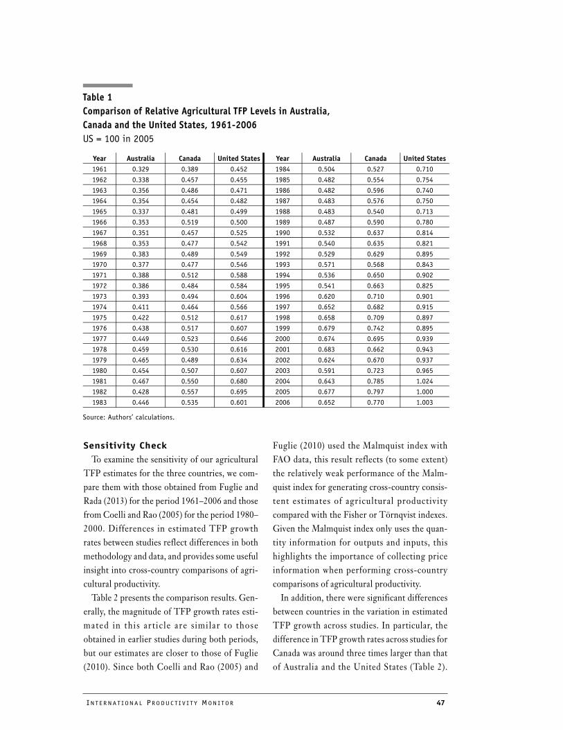
Chart 1

Comparable Agricultural TFP Levels, Australia,

Canada and the United States, 1961-2006

(US=100 in 2005)

Note: Detailed results are shown in Table 1.

Source: Authors’ calculations.

Chart 2

Agricultural TFP Levels Relative to the United States,

1961-2006

(per cent)


46 NUMB E R 29 , FALL 2015

rural areas to approximate the level of rural infra-

structure available to farmers. Specifically, this

variable was defined as the total length of roads in

the rural areas of each country divided by the

rural population. In addition, we also used the

urbanisation ratio, defined as the proportion of

the urban population in the total population, as a

control variable to represent changing economic

development levels in each country. Data used to

construct those variables were obtained from the

World Bank World Development Indicator data-

base, which provides cross-country consistent

measures of these variables.5

Finally, all three countries have significant

shares of non-irrigated cropping and grazing in

their agriculture sectors, hence changes in rainfall

and temperature will affect agricultural produc-

tivity from year to year. To consider these effects,

we used total precipitation and average tempera-

ture for the crop growing season in each country.

Reflecting the difference in seasons between the

Northern and Southern hemispheres, the grow-

ing season for Australia is defined as September

to April while for Canada and the United States it

is defined as March to October. Data used to con-

struct these two variables were obtained from the

Global Historical Climatology Network.

Agricultural TFP EstimatesUsing the index method and production

account data, we estimate and compare agri-

cultural TFP between Australia, Canada, and

the United States. A dynamic panel regression

technique is then used to link the productivity

differences between countries to some of its

potential drivers.

Productivity Comparison Between

Australia, Canada, and the United

States

Australian agricultural TFP was generally

below the level achieved by the United States and

Canada from 1961 to 2006 (although in 2001

Australia’s TFP level briefly exceeded the level

achieved by Canada) (Chart 1), but its growth was

relatively strong. Between 1961 and 2006, the

annual growth rate of agricultural TFP in Austra-

lia was 1.6 per cent a year on average, higher than

in Canada (1.2 per cent a year),6 and only slightly

lower than in the United States (1.8 per cent a

year). Australia’s relatively strong TFP growth

allowed it to improve its TFP level relative to

Canada and to maintain its TFP level at around

70 per cent of the United States (Chart 2).

While Canada and the United States had simi-

lar levels of agricultural TFP during the 1960s,

they have since diverged. The average level of

agricultural productivity in Canada fell to 70 per

cent of that in the United States in 2001, before

rebounding to about 80 by the mid-2000s (Chart

2). A further analysis of productivity growth in

the most recent decade of the dataset showed that

Canada experienced a downturn in agricultural

productivity associated with drought in the early

2000s, but this slowdown was not sustained. In

contrast, Australia experienced a slowdown in

agricultural productivity growth from 1998

onwards. This slowdown widened the TFP gap

between Australian agriculture and its North

American competitors, particularly between 2002

and 2006. This finding is consistent with Sheng,

Mullen and Zhao (2011) who identified a turning

point in broadacre agricultural productivity in

Australia after the mid-1990s, associated with

poor seasonal conditions and a decline in the

intensity of public R&D investment.

5 More details about the database are available at http://data.worldbank.org/data-catalog/world-development-

indicators (World Bank, 2015).

6 This TFP growth rate is consistent with the TFP estimate of 1.0 per cent annually in Canadian crop and

animal production over the 1961-2006 period based on Statistics Canada’s official TFP estimates available

in CANSIM Table 383-0022.


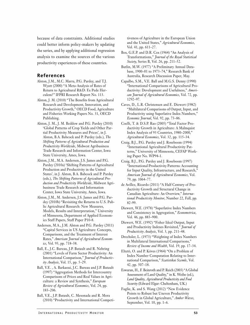
Sensitivity Check

To examine the sensitivity of our agricultural

TFP estimates for the three countries, we com-

pare them with those obtained from Fuglie and

Rada (2013) for the period 1961–2006 and those

from Coelli and Rao (2005) for the period 1980–

2000. Differences in estimated TFP growth

rates between studies reflect differences in both

methodology and data, and provides some useful

insight into cross-country comparisons of agri-

cultural productivity.

Table 2 presents the comparison results. Gen-

erally, the magnitude of TFP growth rates esti-

mated in this artic le are s imi lar to those

obtained in earlier studies during both periods,

but our estimates are closer to those of Fuglie

(2010). Since both Coelli and Rao (2005) and

Fuglie (2010) used the Malmquist index with

FAO data, this result reflects (to some extent)

the relatively weak performance of the Malm-

quist index for generating cross-country consis-

tent estimates of agricultural productivity

compared with the Fisher or Törnqvist indexes.

Given the Malmquist index only uses the quan-

tity information for outputs and inputs, this

highlights the importance of collecting price

information when performing cross-country

comparisons of agricultural productivity.

In addition, there were significant differences

between countries in the variation in estimated

TFP growth across studies. In particular, the

difference in TFP growth rates across studies for

Canada was around three times larger than that

of Australia and the United States (Table 2).

Table 1

Comparison of Relative Agricultural TFP Levels in Australia,

Canada and the United States, 1961-2006

US = 100 in 2005


Year Australia Canada United States Year Australia Canada United States

1961 0.329 0.389 0.452 1984 0.504 0.527 0.710

1962 0.338 0.457 0.455 1985 0.482 0.554 0.754

1963 0.356 0.486 0.471 1986 0.482 0.596 0.740

1964 0.354 0.454 0.482 1987 0.483 0.576 0.750

1965 0.337 0.481 0.499 1988 0.483 0.540 0.713

1966 0.353 0.519 0.500 1989 0.487 0.590 0.780

1967 0.351 0.457 0.525 1990 0.532 0.637 0.814

1968 0.353 0.477 0.542 1991 0.540 0.635 0.821

1969 0.383 0.489 0.549 1992 0.529 0.629 0.895

1970 0.377 0.477 0.546 1993 0.571 0.568 0.843

1971 0.388 0.512 0.588 1994 0.536 0.650 0.902

1972 0.386 0.484 0.584 1995 0.541 0.663 0.825

1973 0.393 0.494 0.604 1996 0.620 0.710 0.901

1974 0.411 0.464 0.566 1997 0.652 0.682 0.915

1975 0.422 0.512 0.617 1998 0.658 0.709 0.897

1976 0.438 0.517 0.607 1999 0.679 0.742 0.895

1977 0.449 0.523 0.646 2000 0.674 0.695 0.939

1978 0.459 0.530 0.616 2001 0.683 0.662 0.943

1979 0.465 0.489 0.634 2002 0.624 0.670 0.937

1980 0.454 0.507 0.607 2003 0.591 0.723 0.965

1981 0.467 0.550 0.680 2004 0.643 0.785 1.024

1982 0.428 0.557 0.695 2005 0.677 0.797 1.000

1983 0.446 0.535 0.601 2006 0.652 0.770 1.003

48 NUMB E R 29 , FALL 2015

This difference might reflect the use of different

data sources in earlier studies, which reinforces

the importance of constructing a production

account that is comparable across countries

when performing international comparisons of

agricultural productivity.

Agricultural TFP DriversEstimation Strategy for

TFP Driver Analysis

To investigate cross-country differences in

agricultural productivity, we use a dynamic

panel data regression to analyse the relationship

between TFP measures and some potential driv-

ers. Following Alston et al. (2010a), Ball et al.

(2001, 2010) and OECD (2012), we focus on

three such drivers, namely technological

progress, capital deepening and the availability

of infrastructure, while controlling for the

impacts of climate conditions and the market

environment. The empirical specification is, for

simplicity, assumed to take the log-linear form

so that we can interpret coefficients in terms of

percentage changes in TFP:

(7)

where is the logarithm of agricultural

TFP of country i at year t. denotes the log-

arithm of potential drivers of productivity across

countries, denotes the control variables

and are the residuals. and are the coef-

ficients associated with productivity drivers and

control variables respectively, which capture their

marginal effects on agricultural productivity. The

null hypothesis is that is insignificant, suggest-

ing that there is no causal relationship between

the potential drivers and cross-country produc-

tivity growth and vice versa.

Implementing equation (7) may encounter

potential endogeneity problems because of pos-

sible correlation between independent variables

and the residual. To avoid this problem, we use a

flexible combination of lagged independent

variables and the differential of rainfall and tem-

perature as instruments,7 and adopt the general-

ized method of moments (GMM) to perform the

estimation. A difference GMM is used as it elim-

7 Our argument for using the differential of exogenous climate change conditions as a valid instrument is based

on the observation of significant amount of efforts having been put into dealing with adaptation to climate

change at the national levels for all the three countries. Specifically, lagged and differential of those variables

generally will not directly affect agricultural productivity of the current period when land quality is well con-

trolled (when TFP are estimated). But, they are correlated to rainfall and tempreture in the current period,

given that the climate is gradually evolving over time (or time-contigent). In addition, when observing rain-

fall and temperature in the previous period, farmers are willing to adapt to the situation through changing

R&D knowledge stock, infrastructure, capital-labor ratio to adapt to the new environment.

TFPitln β0 βj Xitj γk Zit

k εit+ln

k

∑+ln

j

∑+=

TFPitln

X.,.j

ln

Z.,.k

ln

εit βj γk

βj

Table 2

Agricultural TFP Growth Rates

(per cent)

Note: TFP growth rates are estimated using the regession method.

Australia Canada United States

Time period for comparison: 1961-2006

Fuglie (2010) 1.53 1.57 1.67

Our estimates 1.64 1.24 1.80

Relative difference to our estimates -0.07 0.27 -0.07

Time period for comparison: 1980-2000

Coelli and Rao (2005) 2.60 3.30 2.60

Our estimates 2.14 1.73 1.99

Relative difference to our estimates 0.21 0.91 0.31


inates country-specific fixed effects. In addition,

we have also use the Arellano-Bond test to

examine autocorrelation of the error terms8 and

the Sargan/Hansen test to examine the identifi-

cation issues.9

Three scenarios are specified. In scenario one

(Model 1), we consider a baseline model which

only incorporates the variables that represent

climate conditions into the regression. Scenario

two (Models 2-4) individually adds disembodied

technological progress, the capital-labour ratio

and infrastructure-related variables into the

baseline model to explore their roles in explain-

ing cross-country productivity differences. Sce-

nario three (Model 5) adds all these factors

together into the baseline model and investi-

gates their combined effects.

A Dynamic Panel Data

Regression Analysis

Many factors have been used to explain differ-

ences in agricultural productivity between coun-

tr ies . These include cl imate condi t ions ,

technological progress and innovation, public

infrastructure and domestic policies (Alston,

Beddow and Pardey, 2010; Ball et al., 2010;

OECD 2012). In this research, a dynamic panel

regression analysis was used to estimate the rel-

ative contribution of these factors to agricultural

productivity growth based on annual data for the

1961-2006 period for Australia, Canada, and the

United States. Reflecting concerns on the lim-

ited sample size, standard errors were corrected

(by using the finite-sample regression proce-

dure) to avoid the potential for downward bias

(Windmeijer, 2005) and country-specific cluster

effects were accounted for. The results obtained

from different scenarios, and the corresponding

Arrellano-Bond test and the Sargan/Hansen

tests are reported in Table 3. Three main find-

ings are discussed below.

First, R&D spending has played an important

role in promoting agricultural productivity

growth across the three countries. After control-

ling for climate conditions and services from pub-

lic infrastructure, the coefficients associated with

R&D knowledge stocks (which generate the ser-

vice flow of disembodied technologies) are 0.34

and 0.35, which are positive and significant at the

1 per cent level. The results are consistent

throughout different scenarios (Models 2 and 5),

implying that a one per cent increase in the R&D

knowledge stock tends to raise the agricultural

TFP level by more than 0.3 per cent. Similar

results were also obtained in Alston et al. (2000),

Pardey et al. (2006) and Alston (2010), which

showed productivity improvements in agriculture

were strongly associated with lagged R&D

investments. This suggests that further increas-

ing agricultural R&D investment remains an

effective way for policy makers to achieve long-

term productivity growth in agriculture.

Second, simply increasing the capital-labour

ratio without adopting new technology and

changing farm practices does not necessarily

increase agricultural TFP in the three countries.

In our regressions, the coefficients attached to

the capital-labour ratio are not significant at the

10 per cent level and become negative when

other factors are accounted for (Column 5 in

Table 3). This implies that increasing the capi-

tal-labour ratio through making more invest-

ment does not necessar i l y contr ibute to

improved TFP levels.10 For example, to imple-

ment reduced-till technology in the cropping

industry, farmers in Australia, Canada, and the

8 The Arrellano-Bond test is designed to examine whether there is autocorrelation in the idiosyncratic distur-

bance term, and helps to identify which periods of lagged variables could be used to obtain instruments. The

null hypothesis is that once fixed effects are removed, the disturbance term is not autocorrelated.

9 The Sargan/Hansen tests are designed to examine whether the model is over-identified, and tests for the

joint validity of the moment conditions in the GMM framework. The null hypothesis of these tests are that

the chosen moments (or instruments) are jointly valid.

50 NUMB E R 29 , FALL 2015

United States invested heavily in more powerful

tractors/machinery and larger pieces of land

during the 1980s and 1990s. By the 2000s, how-

ever, this technology was widely adopted, and

further investment in powerful tractors/machin-

ery encountered decreasing marginal rates of

return, particularly on farms with relatively

modest size (Sheng et al., 2015).

Although this finding appears inconsistent

with that of Ball et al. (2001), who found that an

increase in the capital-labour ratio significantly

contributed to reducing the difference in agri-

cultural productivity between European coun-

tries and the United States, it is nonetheless a

reasonable result. On one hand, all three coun-

tries in this analysis have been widely adopting

capital-intensive technologies such as minimum

or no tillage and yield mapping for some time,

and accordingly, further investment in physical

capital may lead to decreasing marginal returns

to capital. As such, labour and land productivity

can still increase with more investment, but total

factor productivity will decline. On the other

hand, a positive correlation between a change in

the capital-labour ratio and agricultural TFP in

Ball et al. (2001) could result from the interac-

tion between the capital-labour ratio and other

productivity drivers (i.e . R&D knowledge

stock), which have not been well considered in

this study. Empirically, this follows from the

observation that the marginal effects of the cap-

ital-labour ratio on productivity become nega-

tive when other variables are controlled for

(Models 3 and 5 in Table 2).

10 Of course, increased capital intensity boosts labour productivity. For example, de Avillez (2011) showed that

capital deepening accounted for just under one half of the 3.77 per cent increase in output (value added) per

hour in Canadian agriculture between 1961 and 2007.

Table 3

Dynamic Panel Regression on Agricultural TFP Levels, Difference GMM Estimation Results

Note: the numbers in parenthesis below coefficients are “robust” standard errors taking into consideration of heterosk-

edasticity H(1), and *** p<0.01, ** p<0.05, * p<0.1. Statistics for Arrellanno-Bond test for autocorrelation and

Sargan/Hansen test for over identification are p-values.

Scenario 1 Scenario 2 Scenario 3

Model 1 Model 2 Model 3 Model 4 Model 5

Dependent variable: lnTFP

ln_rainfall (growing seasons) 0.056**

(0.027)

0.054**

(0.027)

0.058**

(0.028)

0.056**

(0.004)

0.051***

(0.005)

ln_average_temp 0.068***

(0.013)

0.064***

(0.015)

0.071***

(0.010)

0.069***

(0.007)

0.068***

(0.009)

ln_R&D knolwedge stock-

0.337***

(0.082)- -

0.349***

(0.112)

ln_capital_labour_ratio- -

0.061

(0.065)-

-0.001

(0.039)

ln_infrastructure_index- - -

0.179***

(0.013)

0.196***

(0.013)

urbanisation ratio- - -

0.059*

(0.031)

0.031**

(0.014)

Number of observations 135 135 135 135 135

F-statistics 417 1,148 262 217 321

Arrellano-Bond test for AR(1) 0.191 0.164 0.196 0.111 0.119

Arrellano-Bond test for AR(2) 0.331 0.235 0.308 0.461 0.406

Sargan test of overid. restrictions 1.000 0.424 0.426 0.388 0.341

Hansen test of overid. restrictions 1.000 1.000 1.000 1.000 1.000


Third, climate conditions and public poli-

cies targeted to improve the supply of public

infrastructure services may also contribute to

explaining cross-country differences in TFP

growth. In all scenarios, the coefficients esti-

mated for growing-season rainfall and tem-

perature are positive and significant at the 1-5

per cent level (Models 1 and 5 in Table 3).

This suggests that agricultural TFP is sensi-

tive to average growing-season rainfall and

temperature in the three countries, which

implies that differences in climate condition

could be causes of differences in TFP growth.

In addition, the results also show that the

availability of public infrastructure and the

urbanisation ratio (a proxy for the level of

economic development) appear to have posi-

tive impacts on productivity. For example, the

coefficients associated with the rural infra-

structure index and the urbanisation ratio are

all positive and significant at the 1-10 per cent

level (Models 4 and 5 in Table 3).

Robustness Check

To establish whether or not the findings

obtained from the analysis of productivity driv-

ers are sensitive to the choice of methods and the

independent variables included, we carried out

two robustness tests.

First, with respect to the choice of regression

methods, it has been argued that the dynamic

panel data regression technique is less efficient

than the standard panel data regression technique

when a long time-series of data is available (Zilak,

Table 4

Robustness Checks on Estimation Method and Variable Choices

Note: the numbers in parenthesis below coefficients are “robust” standard errors that account for heterochasticity

H(1), and *** p<0.01, ** p<0.05, * p<0.1. Statistics for Arrellanno-Bond test for autocorrelation and Sargan/

Hansen tests for over identification are p-values.

Scenario 1 Scenario 2

Panel Fixed Effect Panel Fixed Effect Difference GMM

Dependent variable: lnTFP

ln_rainfall (growing seasons) 0.098***

(0.008)

0.135***

(0.008)

0.138***

(0.008)

ln_average_temp 0.062***

(0.005)

0.063***

(0.004)

0.062***

(0.005)

R&Dknowledgestock 0.316***

(0.057)

0.213***

(0.039)

0.231***

(0.038)

ln_capital_labour_ratio -0.018

(0.043_

-0.050

(0.046)

-0.053

(0.046)

ln_infrastructure_index 0.304***

(0.059)

0.350***

(0.050)

0.354***

(0.050)

urbanisation_ratio 0.043***

(0.010)

-0.037***

(0.010)

0.037***

(0.009)

similarity_index-

0.838***

(0.154)

0.885***

(0.155)

Constant 1.586***

(0.450)

0.458***

(0.028)-

Number of observations 138 138 135

Adjusted R-squared 0.883 0.901 -

Arrellano-Bond test for AR(1) - - 0.150

Arrelanno-Bond test for AR(2) - - 0.101

Sargan test of overid. restrictions - - 0.350

Hansen test for overid. restrictions - - 1.000

52 NUMB E R 29 , FALL 2015

1997; Wooldridge, 2010). To check the sensitivity

of our finding to the regression method used, we

re-estimated equation (7) using a panel data

regression with fixed effects (for Scenario 1 in

Table 4). The results obtained from this regres-

sion are similar to those obtained from the

dynamic panel data regression.

Second, with respect to the choice of inde-

pendent variables, it could be argued that the

three countries produce different mixes of

output, and produce some country-specific

products , which may bias the regress ion

results. For example, Canada and the United

States produce a large amount of maize and

soybeans in the crop sector and beef and cattle

in the livestock sector while Australia pro-

duces more canola in the crop sector and more

sheep and wool in the livestock sector. With-

out accounting for this disparity in output mix

between countries, the estimated contribution

of var ious product iv i ty dr ivers would be

biased since TFP could vary between farms.

To examine the sensitivity of our findings to

this possibility, we added an index of output

similarity to the regression.11 The results are

similar to those obtained from the basic

model, although model fit is higher.

ConclusionThis article has estimated and compared agricul-

tural total factor productivity in Australia, Canada

and the United States between 1961 and 2006. To

do this, a consistent production account for the

agriculture sector in all three countries was devel-

oped, and a multilateral index was applied to con-

struct comparable price and quantity estimates for

output and input in each country.

Our results show that these countries have expe-

rienced different TFP levels and growth patterns

over the past four decades, despite primarily using

capital-intensive technologies and possessing simi-

larly well-developed production systems. In partic-

ular, Australian agriculture has experienced rapid

productivity growth over four decades, which has

improved Australia’s productivity level relative to

Canada and maintained it relative to the United

States. In recent years however, Australia’s produc-

tivity growth rate has slowed relative to that of

Canada and the United States.

Further empirical analysis shows that agricul-

tural productivity differences are likely to be

related to each country’s capacity for investing

in R&D and the availability of infrastructure.

Differences in climate conditions are also found

to be important causes of differences in agricul-

tural TFP between Australia, Canada, and the

United States. These findings provide useful

insights into the importance of public policies in

promoting public R&D investment in agricul-

ture and providing infrastructure to the farm

sector to sustain productivity growth.

Although our estimates measure agricultural

output, input and TFP in the three countries, a

shortcoming is that the time series ends at 2006

11 An output similarity index relative to the US at the base year (i.e. 2005) was estimated for Australia, Canada,

and the United States based on all agricultural outputs. The output similarity index ( ) is given by

where and are the value of production of output m, expressed as a

share of the total value of agricultural output in country i (that is, Australia, Canada or the United States) at

time t and country j (that is, the United States at the based year 2005) where there is a total of M different

commodity categories for Australia (or Canada) and the United States, and M = 16. Data on for Australia,

Canada and the United States, and data on for the United States at the base year are obtained from the

output value estimates at current prices. For a more detailed technical discussion, see Alston, Beddow and

Pardey (2010).

ω

ω

fimfjm

m 1=

M

∑

fim

2( )1 2⁄

fjm

2( )1 2⁄

m 1=

M

∑m 1=

M

∑

-------------------------------------------------------------------= fim fjm

fim

fjm


because of data constraints. Additional studies

could better inform policy-makers by updating

the series, and by applying additional regression

analysis to examine the sources of the various

productivity experiences of these countries.

ReferencesAlston, J.M., M.C. Marra, P.G. Pardey, and T.J.

Wyatt (2000) “A Meta-Analysis of Rates of Return to Agricultural R&D: Ex Pede Her-culem?” IFPRI Research Report No. 113.

Alston, J. M. (2010) “The Benefits from Agricultural Research and Development, Innovation, and Productivity Growth,” OECD Food, Agriculture and Fisheries Working Papers No. 31, OECD Publishing.

Alston, J. M., J. M. Beddow and P.G. Pardey (2010) ‘Global Patterns of Crop Yields and Other Par-tial Productivity Measures and Prices’, in J. Alston, B.A. Babcock and P. Pardey (eds.), The Shifting Patterns of Agricultural Production and Productivity Worldwide, Midwest Agribusiness Trade Research and Information Center, Iowa State University, Ames, Iowa.

Alston, J.M., M.A. Andersen, J.S. James and P.G. Pardey (2010a) ‘Shifting Patterns of Agricultural Production and Productivity in the United States’, in J. Alston, B.A. Babcock and P. Pardey (eds.), The Shifting Patterns of Agricultural Pro-duction and Productivity Worldwide, Midwest Agri-business Trade Research and Information Center, Iowa State University, Ames, Iowa.

Alston, J.M., M. Andersen, J.S. James and P.G. Par-dey (2010b) “Revisiting the Returns to U.S. Pub-lic Agricultural Research: New Measures, Models, Results and Interpretation,” University of Minnesota, Department of Applied Econom-ics Staff Papers, Staff Paper P10-8.

Andersen, M.A., J.M. Alston and P.G. Pardey (2011) “Capital Services in US Agriculture: Concepts, Comparisons, and the Treatment of Interest Rates,” American Journal of Agricultural Econom-ics, Vol. 93, pp. 718–38.

Ball, E., J.C. Bureau, J.P. Butault and R. Nehring (2001) “Levels of Farm Sector Productivity: An International Comparison,” Journal of Productiv-ity Analysis, Vol. 15, pp. 5–29.

Ball, V.E. , A. Barkaoui, J.C. Bureau and J.P. Butault (1997) “Aggregation Methods for Intercountry Comparisons of Prices and Real Values in Agri-culture: a Review and Synthesis,” European Review of Agricultural Economics, Vol. 24, pp. 183–206.

Ball, V.E., J.P. Butault, C. Mesonada and R. Mora (2010) “Productivity and International Competi-

tiveness of Agriculture in the European Union and the United States,” Agricultural Economics, Vol. 41, pp. 611–27.

Box, G.E.P. and D.R. Cox (1964) “An Analysis of Transformations,” Journal of the Royal Statistical Society, Series B, Vol. 26, pp. 211–52.

Butlin, M.W. (1977) “A Preliminary Annual Data-base, 1900–01 to 1973–74,” Research Bank of Australia, Research Discussion Paper, May.

Capalbo, S.M., V.E. Ball and M.G.S. Denny (1990) “International Comparisons of Agricultural Pro-ductivity: Development and Usefulness,” Ameri-can Journal of Agricultural Economics, Vol. 72, pp. 1292–97.

Caves, D., L.R. Christensen and E. Diewert (1982) “Multilateral Comparisons of Output, Input, and Productivity using Superlative Index Numbers,” Economic Journal, Vol. 92, pp. 73–86.

Coelli, T. & D.S.P. Rao (2005) “Total Factor Pro-ductivity Growth in Agriculture: A Malmquist Index Analysis of 93 Countries, 1980–2000,” Agricultural Economics, Vol. 32, pp. 115–34.

Craig, B.J., P.G. Pardey and J. Roseboom (1994) “International Agricultural Productivity Pat-terns,” University of Minnesota, CEFAP Work-ing Paper No. WP94-1.

Craig, B.J., P.G. Pardey and J. Roseboom (1997) “International Productivity Patterns: Accounting for Input Quality, Infrastructure, and Research,” American Journal of Agricultural Economics, Vol. 79, pp. 1064–77.

de Avillez, Ricardo (2011) “A Half Century of Pro-ductivity Growth and Structural Change in Canadian Agriculture: An Overview,” Interna-tional Productivity Monitor, Number 22, Fall, pp. 82-99.

Diewert, W.E. (1978) “Superlative Index Numbers and Consistency in Aggregation,” Econometrica, Vol. 46, pp. 883–900.

Diewert, W.E. (1992) “Fisher Ideal Output, Input and Productivity Indexes Revisited,” Journal of Productivity Analysis, Vol. 3, pp. 211–48.

Drechsler, L. (1973) “Weighting of Index Numbers in Multilateral International Comparisons,” Review of Income and Wealth, Vol. 19, pp. 17–34.

Eltetö, O. and P. Köves (1964) “On a Problem of Index Number Computation Relating to Inter-national Comparison,” Szatistikai Szemle, Vol. 42, pp. 507–18.

Eswaran, H., F. Beinroth and P. Reich (2003) “A Global Assessment of Land Quality,” in K. Weibe (ed.), Land Quality, Agricultural Productivity and Food Security (Edward Elgar: Cheltenham, UK.)

Fuglie, K. and S. Wang (2012) “New Evidence Points to Robust but Uneven Productivity Growth in Global Agriculture,” Amber Waves, September, Vol. 10, pp. 1–6.

54 NUMB E R 29 , FALL 2015

Fuglie, K.O. (2010) “Total Factor Productivity in the Global Agricultural Economy: Evidence from FAO Data,” in J. Alston, B.A. Babcock and P. Pardey (eds.), The Shifting Patterns of Agricultural Production and Productivity Worldwide, Midwest Agribusiness Trade Research and Information Center, Iowa State University, Ames, Iowa, pp. 63–95.

Fuglie, K.O., S. Wang and E. Ball (2012) “Produc-tivity Growth in Agriculture: An International Perspective,” (CAB International: Cambridge, MA.)

Headey, D., M. Alauddin and D.S.P. Rao (2010) “Explaining Agricultural Productivity Growth: An International Perspective,” Agricultural Eco-nomics, Vol. 41, pp. 1–14.

Huffman, W.E. and R.E. Evenson (2006) “Do For-mula or Competitive Grant Funds Have Greater Impacts on State Agricultural Productivity?” American Journal of Agricultural Economics, Vol. 88, pp. 783–98.

Jorgenson, D.W. and P. Schreyer (2012) “Industry-Level Productivity Measurement and the 2008 System of National Accounts,” Review of Income and Wealth, Vol. 59, pp. 185-211.

Ludena, C.E., T.W. Hertel, P.V. Preckel, K. Foster and A. Nin (2007) “Productivity Growth and Convergence in Crop, Ruminant and Non-Ruminant Production: Measurement and Fore-casts,” Agricultural Economics, Vol. 37, pp. 1–17.

Lusigi, A. and C. Thirtle (1997) “Total Factor Pro-ductivity and the Effects of R&D in African Agriculture,” Journal of International Develop-ment, Vol. 9, pp. 529–38.

OECD (2001) “Measuring Productivity: Measure-ment of Aggregate and Industry-Level Produc-tivity Growth,” OECD Manual, OECD, Paris.

OECD (2012) “Cross Country Analysis of Farm Per-formance,” Trade and Agriculture Directorate, Committee for Agriculture, OECD, Paris.

Pardey, P.G., N. Beintema, S. Dehmer and S. Wood (2006) “Agricultural Research: A Growing Glo-bal Divide?” Agricultural Science and Technol-ogy Indicators Initiative, International Food Policy Research Institute, Washington, DC.

Penson, J. B., D. W. Hughes and G. L. Nelson (1987) “Measurement of Capacity Depreciation Based on Engineering Data,” American Journal of Agricultural Economics, Vol. 35, pp. 321–29.

Powell, R. A. (1974) “Technological Change in Aus-tralian Agriculture, 1920–21 to 1969–70,” The-sis, University of New England, Armidale.

Rao, D. S. P, A. Maddison and B. L. Lee (2002) “Inter-national Comparison of Farm Sector Performance: Methodological Options and Empirical Findings for Asia-Pacific Economies, 1900–1994,” in A. Maddison, W.F. Shepherd, and R. Prasada (eds.), The Asian Economies in the Twentieth Century (Edward Elgar, Northampton, MA), pp. 27–52.

Romain, R., J.B. Penson and R. Lambert (1987) “Capacity Depreciation, Implicit Rental Prices, and Investment Demand for Farm Tractors in Canada,” Canadian Journal of Agricultural Eco-nomics, Vol. 35, pp. 373–78.

Sanchez, P.A., C.A. Palm and S.W. Buol (2003) “Fer-tility Capability Soil Classification: A Tool to Help Assess Soil Quality in the Tropics,” Geo-derma, Vol. 114, issues 3–4, pp. 157–85.

Sheng, Y., E. Gray, J.D. Mullen and A. Davidson (2011) “Public Investment in Agricultural R&D and Extension: An Analysis of the Static and Dynamic Effects on Australian Broadacre Pro-ductivity,” ABARES Research Report 11.7, Aus-tralian Bureau of Agricultural and Resource Economics and Sciences, Canberra.

Sheng, Y., J.D. Mullen and S. Zhao (2011) “A Turn-ing Point in Agricultural Productivity: Consider-ation of the Causes,” ABARES Research Report 11.4 for the Grains Research and Research and Development Corporation, Australian Bureau of Agricultural and Resource Economics and Sci-ences, Canberra.

Sheng, Y., S. Zhao, K. Nossal and D. Zhang (2015) “Productivity and Farm Size in Australian Agri-culture: Reinvestigating the Returns to Scale,” Australian Journal of Agriculture and Resource Eco-nomics, Vol. 59. pp. 16-38.

Shi, U. J., T.T. Phipps and D. Colyer (1997) “Agri-cultural Land Values Under Urbanizing Influ-ences,” Land Economics, Vol. 73, pp. 90–100.

Szulc, B. (1964) “Indices for Multiregional Compari-sons,” Przeglad Statystyczny, Vol. 3, pp. 239–54.

World Bank (2007) World Bank Development Report 2008, World Bank, Washington, DC.

World Bank (2015) World Development Indicator Database, World Bank, Washington, DC, avail-able at the website of http://data.worldbank.org/data-catalog/world-development-indicators.

Zilak, J. P. (1997) “Efficient Estimation with Panel Data When Instruments Are Predetermined: An Empirical Comparison of Moment-Condition Estimators”, Journal of Business and Economic Sta-tistics, Vol. 15, pp. 419-431.

Wooldridge, J. (2010) Econometric Analysis of Cross Section and Panel Data, 2nd Edition, (MIT Press: Cambridge, MA).


Appendix A

Cross-Country Consistent Production Account for Agriculture:

Methodology and Variable Definition

The agricultural production account is

defined and collected consistently between

countries, and data are obtained from a range of

sources in each country. This appendix provides

a definition for each output and input (summa-

rized in Table A1). All data were collected on a

calendar year basis. For Australia, this meant

converting financial year data by taking a simple

average of two consecutive financial years.

OutputsOutput variables were collected under three

categories: crops, livestock and other outputs.

Crop outputs included grains and oil seeds, veg-

etables, and fruits and nuts. Livestock outputs

included slaughter livestock (red meat), poultry

and eggs, and other animal products (dairy and

wool). Other outputs included ‘non-separable

secondary activities’ such as income from

machinery hire and contract services.

Primary agricultural outputs included deliver-

ies to final demand as well as intermediate

demand and on-farm use. Primary output is

approximated as total sales plus non-market

transactions (that is, cross-industry transfers

through long-term contracts and on-farm use

such as animal feed). Where production statis-

tics are not directly available, primary output is

approximated from changes in inventory for

each commodity.

Outputs from non-separable secondary activi-

ties are defined as goods and services whose

costs cannot be observed separately from those

of primary agricultural outputs. Two types of

secondary activities are included: on-farm pro-

duction activities such as the processing, pack-

aging and marketing of agricultural products,

and service provision such as machinery hire and

land lease.

Government taxes are included in agricultural

outputs, since the value of inputs is inclusive of

indirect taxes. We recognise that differences in

government subsidies or taxes between coun-

tries may create differences in the measured

value of total output.

Equation (3) is used to aggregate output prices

using their corresponding revenue shares. The

implicit aggregate output quantity index is then

defined as the total value of agricultural output

divided by the aggregate price index.

InputsInput variables were collected under four cat-

egories: capital, land, labour, and intermediate

inputs. Capital and land inputs are estimated as

service flows.

Capital

Following Ball et al. (2001 and 2010), three

types of capital input are distinguished: non-

dwelling buildings and structures, plant and

machinery, and transportation vehicles. While

relevant, the inventory of crops, livestock, and

other biological resources, such as vineyards and

orchards, are not included because of inadequate

value data. However, these capital inputs are

likely to represent a relatively small proportion

of total capital.

Measurement of the capital input begins with

using investment data to calculate the stock of

three types of capital goods. At each point in

time t, the stock of capital K(t) is the sum of all

past investments, , weighted by the relative

efficiencies of capital goods of each age , .

(A1)

It τ–

τ Sτ

Kt SτIt τ–τ 0=

∞

∑=

56 NUMB E R 29 , FALL 2015

When using equation (A1) to estimate the

capital stock, the efficiencies of capital goods

must be defined explicitly. Similar to Ball et al.

(2010), this is done by using two parameters,

namely service life of the asset, L, and a decay

parameter, , to specify the functional form,

S(.) such that:

(A2) , if

if

Each type of capital asset has an assumed

distribution of actual service life which pro-

vides a mean service life . In this analysis, the

asset lives for non-dwelling buildings and

structures, plant and machinery, and transport

and other vehicles are assumed to be 40 years,

20 years and 15 years, respectively, with an

assumed standard normal distribution trun-

cated at points two standard deviations before

and after the mean service life.

The decay parameter can take values

between 0 and 1, with = 1 implying that the

capital asset does not depreciate over its ser-

vice life. Although there is little empirical evi-

dence to define appropriate values of , it is

reasonable to assume that the efficiency of a

capital asset declines smoothly over most of

its service life. Following Ball et al. (2001),

decay parameters are set to be 0.75 for non-

dwelling buildings and structures and 0.50 for

all other capital assets, reflecting an assump-

tion that efficiency declines more quickly in

the later years of service (Penson, Hughes and

Nelson, 1987; Romain, Penson and Lambert,

1987).

The aggregate efficiency function was con-

structed as a weighted sum of individual effi-

ciency functions where the weights are the

frequency of occurrence.

Rental Rate

Assuming the sector invests when the present

value of the net revenue generated by an addi-

tional unit of capital exceeds the purchase price

of the asset, the farm sector will invest in capital

stock formation until the output price P satisfies:

(A3)

where c is the implicit rental price of capital, r

is the real rate of return and is the price of an

additional unit of capital (or investment).

The rental price c consists of two components:

the opportunity cost associated with investment,

, and the present value of the cost of all

future replacements required to maintain the

productive capacity of the capital stock,

.

Let F denote the present value of the rate of

capital depreciation on one unit of capital

according to the mortality distribution m:

(A4)

w h e r e f o r

.

It can be shown that

such that

(A5)

Following Ball et al. (2010), the real rate of

return, r, is approximated with an ex-ante rate,

estimated as the nominal rate of return minus

inflation. The nominal rate of return is obtained

β

S τ( ) L τ–( ) L βτ–( )⁄= 0 τ L≤ ≤

S τ( ) 0= τ L>

L

ββ

β

PδY

δK------

rWK r WK

δRt

δK-------- 1 r+( ) t–

t 1=

∞

∑+ c

=

= =

WK

rWK

WK

δRt

δK-------- 1 r+( ) t–

s

t 1=

∞

∑

F mt 1 r+( ) t–

t 1=

∞

∑=

m τ( ) S τ( ) S τ 1–( )–[ ]–=

τ 1 … L, ,=

δRt

δK-------- 1 r+( ) t–

t 1=

∞

∑ Ft

t 1=

∞

∑F

1 F–-----------= =

crWK

1 F–-----------=


using the exogenous approach, and is derived

from returns on government bonds with a range

of different maturities. The choice of interest

rate is widely debated. Andersen, Alston and

Pardey (2011) argued that use of a fixed interest

rate generates more plausible estimates of capi-

tal services in the United States than annual

market rates, while Jorgenson and Schreyer

(2012) proposed using the residual of output

value after deducting input costs to derive an

endogenous real interest rate. To test the sensi-

tivity of measured capital services to different

real interest rates, both ex-ante and ex-post rates

were estimated. The ex-ante rate was chosen for

this study as it was less volatile than the ex-post

rate.

Land

The value of land service flows is given by the

product of the land stock and rental price. The

stock of land was estimated from the total land

areas operated. The rental price of land was

obtained using Equation (9) with the assump-

tion of zero depreciation, i.e. . As

explained below, the land price, , was derived

from a hedonic function.

In particular, agricultural land prices can be

affected by many factors unrelated to agricul-

tural production, such as urbanisation pressures,

distance to major cities and government land

release policies. Also, spatial differences in land

quality may prevent direct comparison of prices

between regions and over time. To address these

problems, comparable land price indexes for

each country were constructed using the

hedonic regression method.

In this article, the hedonic price of land is a

generalised linear function of its characteristics

relevant to agricultural production and some

control variables. The function uses the Box-

Cox (1964) transformation to represent the

dependent variable and each continuous inde-

pendent variable:

(A6)

where the price of land, , is the Box-Cox

transformation of real observations, when

, that is:

(A7) if

if

Similarly, , a vector of land character-

istics associated with agricultural production, is

the Box-Cox transformation of the continuous

quality variable where:

(A8) if

if

and D is a vector of country dummies used to

control for external factors. For simplicity, D is

approximated by a group of region and time

dummy variables and not subject to transforma-

tion; , and are unknown parameter vec-

tors to be determined in the regression and is

a stochastic disturbance term. This expression

can assume linear, logarithmic and intermediate

nonlinear functional forms depending on the

transformational parameter.

To apply the hedonic regression model,

regional land prices and land characteristics

were observed for each country in 2005. Land

characteristic data for 2005 were sourced from

the USDA World Soil Resources Office and

selected following Eswaran, Beinroth and Reich

(2003) and Sanchez, Palm and Buol (2003). GIS

mapping was used to overlay country and

regional boundaries with land characteristics

data relating to particular soil categories,

including soil acidity, salinity, and moisture

c rWL=

WL

WL λ0( ) αnXnλn γdDd ε+d

∑+n

∑=

WL λ0( )

WL 0>

WL λ0( ) f x( )WL

λ0

λ0

---------= = λ0 0≠

WL λ0( ) f x( ) WLln= = λ0 0=

Xn λn( )

Xn

Xn λn( ) f x( )Xn

λn1–

λn

----------------------= = λ0 0≠

Xn λn( ) f x( ) Xnln= = λ0 0=

λ α γε

58 NUMB E R 29 , FALL 2015

stress. Across the three countries more than 18

common variables were used to capture environ-

mental attributes.

Two additional attributes affecting the price

of agricultural land should also be considered:

irrigation and population accessibility. Irriga-

tion (the percentage of cropland irrigated) was

included as a separate indicator of production

capacity in water-stressed areas, as well as an

interaction term between irrigation and soil

acidity. A population accessibility index could be

used to control for the impact of urbanisation

and economic development on land prices; how-

ever, it was not included in this analysis due to

data constraints. Such indexes have been con-

structed in previous studies by using a gravity

model of urban development, and provided a

measure of accessibility to population concen-

trations (Shi, Phipps and Colyer, 1997).

Intermediate Inputs

Intermediate inputs comprise all materials

and services consumed, excluding fixed capital,

land and labour inputs. They include 10 catego-

ries, namely: fuel, electricity, fertilisers and

chemicals, fodder and seed, livestock purchases,

water purchases, marketing services, repairs and

maintenance, plant and machinery hire, and

‘other materials and services’.

Fuel (including lubricants) and electricity are

estimated from the total quantity consumed and

an index of prices paid by farmers for petrol, die-

sel, liquefied natural gas and electricity. A fuel

price index was calculated using quantities of

petrol, diesel and liquefied natural gas consumed

as weights. The total quantity of fuel consumed

was obtained by dividing total expenditure by this

fuel price. The price of electricity was estimated

separately and used to deflate electricity expendi-

ture to obtain the quantity consumed.

Other intermediate inputs were estimated as

implicit quantities. Price indexes were sourced

domestically, except for pesticides and chemicals

where quality-adjusted price data from 2005

were sourced from the World Bank World

Development Indicator database and FAO sta-

tistics. The quality-adjusted data for 2005 were

used with domestic time-series prices to impute

a trend.

Consistent with the treatment of output,

intermediate inputs were valued at farm-gate

prices, including direct taxes and excluding indi-

rect taxes and subsidies.

Labour

Labour is defined as total hours worked by

hired, self-employed and unpaid family workers.

Because data were only available on the number

of people employed in the agriculture industry,

total hours worked were imputed by multiplying

the number of workers by the average hours

worked per week and the number of weeks. For

consistency, we use 52 weeks a year for this

imputation.

Wages were not used to estimate the value

share of labour inputs. This is because hourly

wages are unlikely to capture total compensa-

t i on to f a rm worke r s , s i n c e a dd i t i ona l

employee benefits (such as lodging and super-

annuation contributions) are not included in

wage statistics. In addition, compensation to

self-employed workers is not directly observ-

able.

Instead, the real cost of total labour use was

derived using the accounting assumption that

the value of total output equals the value of total

input. This enabled real wages to be estimated as

real labour compensation (or total output value

minus capital, land, and intermediate input

costs) divided by the total number of hours

worked.

Finally, hired, self-employed, and unpaid fam-

ily workers were distinguished, and differences

in education levels and work experience were

used to adjust prices for labour quality in all

three countries.


Table A1

Summary List of Variables

Outputs Inputs

Crops

LivestockOn-farm activities Land Capital Labour Materials

Grains and oil seeds

Fruits and nuts Vegetables

BarleyCanolaCasterCottonseedFlaxseedHay and silageMaizeOatsPeanutRiceRyeSafflowerSorghumSoybeanSunflowerTriticaleWheat

AlmondsApplesApricotsAvocadoesBananasCherries (sweet)Cherries (tart)CranberryDatesFigsGrapefruitGrapesHazelnutsLemons and limesMacadamiasMandarinsMangoesNectarinesOlivesOrangesPeachesPearsPecansPlumsPrunesStrawberriesTangelosTangerinesWalnutsOther fruit and nuts

Asparagus (fresh, processing)Snap beansBean (dry, processing)BroccoliCauliflowerCabbageCapsicumCeleryCucumber (fresh, processing)Corn (fresh, processing)HoneydewLettuceLentilsOnionsPeas (dry, green)PotatoesRock melonSpinach (fresh, processing)Sweet potatoesTomatoes (fresh, processing)WatermelonOther vegetables

Cattle and calvesDucksChickens and broilersEggsHogsMilk, butter, cheeseSheep and lambsTurkeyWool

MarketingPackagingProcessing

Land services Buildings and structures (non-dwelling)Plant machineryTransportation and other vehicles

Operator labourHired labourUnpaid workers

ChemicalsElectricityFertiliserFodder and seedFuel and lubricantLivestock purchasesWater purchasesOther materials

Services

Contract servicesMachinery hireLand leaseOther services

Services

MarketingPlant and machinery hireRepairs and maintenanceVeterinary servicesOther services

Other crops

Cotton lintTobaccoHorticultureFloricultureGreenhouse nurserySugar beetSugar caneMushrooms

Other crops not inlcuded elsewhere

comparing agricultural total factor productivity between ... · comparing agricultural total factor...

Documents