comparing geometric and kinetic cluster algorithms for

Comparing geometric and kinetic cluster algorithms for molecularsimulation data

Bettina Keller,1,a� Xavier Daura,2 and Wilfred F. van Gunsteren1,b�

1Laboratory of Physical Chemistry, Swiss Federal Institute of Technology, ETH, CH-8093 Zürich,Switzerland2Catalan Institution for Research and Advanced Studies (ICREA) and Institute of Biotechnology andBiomedicine (IBB), Universitat Autònoma de Barcelona, 08193 Bellaterra, Barcelona, Spain

�Received 31 January 2009; accepted 8 January 2010; published online 19 February 2010�

The identification of metastable states of a molecule plays an important role in the interpretation ofmolecular simulation data because the free-energy surface, the relative populations in this landscape,and ultimately also the dynamics of the molecule under study can be described in terms of thesestates. We compare the results of three different geometric cluster algorithms �neighbor algorithm,K-medoids algorithm, and common-nearest-neighbor algorithm� among each other and to the resultsof a kinetic cluster algorithm. First, we demonstrate the characteristics of each of the geometriccluster algorithms using five two-dimensional data sets. Second, we analyze the molecular dynamicsdata of a �-heptapeptide in methanol—a molecule that exhibits a distinct folded state, a structurallydiverse unfolded state, and a fast folding/unfolding equilibrium—using both geometric and kineticcluster algorithms. We find that geometric clustering strongly depends on the algorithm used andthat the density based common-nearest-neighbor algorithm is the most robust of the three geometriccluster algorithms with respect to variations in the input parameters and the distance metric. Whencomparing the geometric cluster results to the metastable states of the �-heptapeptide as identifiedby kinetic clustering, we find that in most cases the folded state is identified correctly but the overlapof geometric clusters with further metastable states is often at best approximate. © 2010 AmericanInstitute of Physics. �doi:10.1063/1.3301140�

I. INTRODUCTION

Molecular simulation techniques, such as molecular dy-namics �MD� or Monte Carlo �MC�,1 are powerful tools forthe elucidation of the microscopic structure and the dynam-ics of biomolecules and for the elucidation of the function-ality associated with the former two. As raw output, thesesimulations typically produce a large Boltzmann-weightedensemble of molecular structures or statistical mechanicalconfigurations which serve as the basic data set for furtheranalysis. If one is solely interested in some average over theensemble, it can be calculated without further detailed analy-sis. If one would �additionally� like to organize and concep-tualize this enormous structural data set in order to under-stand �i� which parts of the configurational space areaccessible to the molecule at a given temperature, �ii� howthe molecule moves within this space, and �iii� how theseparts and movements eventually connect to particular mac-roscopic and microscopic properties, clustering of the largeamount of configurational data in one way or the other is anecessity. In this context, the term conformation is used todescribe a �small� part of the configurational space or a sub-set in the configurational ensemble that comprises of struc-turally related configurations. In small molecules the confor-mations are usually defined such that they represent a

minimum in the free-energy surface, i.e., a metastable state,and that different conformations are separated by significantbarriers from each other. It is, however, important to pointout that there is no exact definition of how to map a givenconfigurational or structural ensemble onto different confor-mations.

For small molecules, such as n-butane, CH3�CH2�2CH3,conformational assignment can be done based on a some-what intuitive insight into the molecule’s conformationalspace. According to this insight, the largest barriers inn-butane will occur along the C1–C2–C3–C4-dihedral angle� and the molecule’s conformational isomers are gauche ��with ��60°, trans with ��180°, and gauche �+� with ��300°, of which the trans-conformation is the lowest inenergy because in this conformation the two CH3 units arefarthest apart from each other. The strength of this descrip-tion becomes immediately obvious if one acknowledges thefact that n-butane has N=14 atoms and therefore 3N−6=36 internal configurational degrees of freedom. This high-dimensional space is projected onto only three states whichsuffice to accurately describe the molecule’s free-energylandscape, the relative populations in this landscape, and thedynamics of the molecule.

For larger molecules, such an intuitive partitioning of thestructural ensemble becomes impossible due to the enormoussize and complexity of the configurational space. Conse-quently, also the term conformation becomes fuzzier. Fre-quently, one resorts to grouping structures according to con-formational similarity using geometric cluster algorithms and

a�Electronic mail: [email protected]�Author to whom correspondence should be addressed. Electronic mail:

[email protected].

THE JOURNAL OF CHEMICAL PHYSICS 132, 074110 �2010�

0021-9606/2010/132�7�/074110/16/$30.00 © 2010 American Institute of Physics132, 074110-1

Author complimentary copy. Redistribution subject to AIP license or copyright, see http://jcp.aip.org/jcp/copyright.jsp

http://dx.doi.org/10.1063/1.3301140

http://dx.doi.org/10.1063/1.3301140

http://dx.doi.org/10.1063/1.3301140

refers to the resulting clusters as conformations.2,3 In thissense, the term conformation merely denotes a subensembleof structures that are more similar to each other than to theremaining structures of the ensemble according to a givensimilarity measure. In order to interpret these results, it isthen often �tacitly� assumed that these clusters also representmetastable states.4,5 The underlying assumption here is thatlarge conformational changes are likely to be hindered bybarriers in the free-energy surface, whereas structures thatpopulate a common minimum in the free-energy surfaceshould be conformationally similar. Although these assump-tions seem reasonable at a first glance, there is no guaranteethat they are correct for all types of molecules. As a matter offact, there are known cases in which large movements of,e.g., side chains or other flexible parts of a molecule arehardly hindered by any barrier.6,7 If such a behavior is knownor suspected for a molecule, the problem is commonlyevaded by adapting the similarity measure, thereby introduc-ing a certain arbitrariness into the conformational analysis.For example, when structurally clustering small peptideswith an eye to the �un�folding equilibrium, one typically in-cludes only the backbone atoms or C�-atoms of the centralamino residues and neglects the movement of the side chainsand the terminal residues.

In order to extract information such as relative free en-ergies, rates of conformational changes, or folding pathwaysfrom MD simulations, it is essential to know the basins ofthe free-energy surface as precisely as possible. A basin canbe either described as a region in phase space which is sur-rounded by free-energy barriers or—in terms oflifetimes—as a region in phase space in which a molecule islikely to stay for a long time, i.e.,

tii�� tij�� , �1�

where tii denotes the probability to stay in region i for a timeperiod �� and tij denotes the transition probability of goingfrom region i to region j within time ��. Note that Eq. �1�represents a clear definition of the term metastable state,which is independent of the size of the molecule. The linkbetween free-energy barrier heights and transition probabili-ties can be understood with help of the Arrhenius equation,which states that the rate kij of going from state i to j de-creases exponentially as the barrier between the two states,the activation energy Eij, increases,

kij = A exp�−Eij

RT� , �2�

where A is a prefactor that depends on the system, R is thegas constant, and T is the temperature. In other words, if astate i is surrounded by large barriers, all rates kij are smalland the probability of staying in i for a long period of time ishigh.

Although the term metastable state has a precise defini-tion, actually assessing the metastable states of a large mol-ecule proves to be challenging and rather costly.8–10 In orderto identify metastable states, the phase space—usually re-duced to the molecule’s conformational subspace—is dis-cretized into the so-called microstates, where the term mi-crostates simply denotes a very small part of the phase

space.9 These states are then grouped together into meta-stable states according to kinetic proximity, i.e., the transitionprobability of one microstate to another microstate of thesame group should be much higher than the transition prob-ability to a microstate outside the group—a technique towhich we will refer as kinetic clustering.8–12 The reason whythis procedure is costly is that the transition probabilitiesbetween all pairs of microstates have to be sampled to con-vergence, whereas in geometric clustering, only the confor-mational space has to be sampled with the appropriateweights. Nevertheless, kinetic clustering is—in principle—capable of directly identifying the metastable states of a mol-ecule.

In this contribution, we first wish to assess how sensitivethe geometric cluster results are with respect to the choice ofthe algorithm and its parameters and with respect to thechoice of the similarity measure. Second, we wish to testhow accurately geometric cluster algorithms reproduce themetastable states. To this end, we cluster 15 000 structures ofa �-heptapeptide obtained from a MD simulation using threedifferent geometric cluster algorithms and compare the re-sults. Then, we identify the metastable states of the moleculeby kinetic clustering and using 20 trajectories of a length of500 ns, each of which started from a different initial configu-ration. We sort the data set that was used for the geometricclustering into these metastable states and compare the resultto the clusters obtained using the geometric cluster algo-rithms.

II. THEORY

A. Geometric cluster algorithms

In geometric cluster algorithms, data points are literallyunderstood as points in a �potentially high-dimensional�space for which some distance metric is defined.13 The goalof the algorithm is then to partition a data set S into smallersets �s1 ,s2 ,s3 , . . . such that the distances between the datapoints of a given set are smaller than their distances to datapoints in any other set,

S = �s1,s2,s3, . . . ,sc . �3�

These sets are called “clusters.” We only consider nonfuzzycluster algorithms, that is, algorithms that sort data pointsinto disjoint clusters,

si � sj = 0 ∀ i, j with i � j . �4�

Given a distance measure dij between two data points i and j,a distance matrix D for all pairwise distances in S can beconstructed. In principle, this distance matrix then has to bepermuted in such a way that it takes an approximately block-diagonal form, where the blocks represent the clusters andthe matrix elements in the blocks should be smaller than allother matrix elements,

D� = PDP−1. �5�

Due to the sheer number of possible permutations—theygrow with n!, where n is the number of data points in S—itis usually impossible to find the optimal permutation in abrute force manner. Instead, geometric cluster algorithms

074110-2 Keller, Daura, and van Gunsteren J. Chem. Phys. 132, 074110 �2010�


rely on a number of iterative schemes and different conver-gence criteria.14,15

We tested and compared three different types of geomet-ric cluster algorithms, the first one being the neighbor algo-rithm, as described in Ref. 4. This is a very simple and fastalgorithm in which the neighbors of a data point i are definedto be those data points that lie within a �predefined� distancefrom i. The data point with the most neighbors is consideredto be the medoid of the first cluster and all its neighbors aremembers of the cluster. After the first cluster has been found,all its members are removed from the data pool and the al-gorithm is iterated until all data points have been assigned toa cluster. The algorithm has one parameter: the distance cut-off c, which represents the radii of the clusters. The neighborapproach has the advantage that one does not need to keepthe entire distance matrix in the working memory of thecomputer, it rather suffices to store a list of neighbors foreach data point. This allows the processing of large data setsand makes the algorithm very fast.

The second algorithm we tested is the K-medoids algo-rithm, which belongs to the class of partitioning cluster al-gorithms. These algorithms assign in an initialization step alldata points to a predefined number of clusters and then itera-tively optimize the assignment until some convergence crite-rion is reached. Partitioning algorithms have the advantagethat wrong cluster assignments made in the course of thealgorithm have the chance to be corrected during a later it-eration. However, they need the total number of clusters k asan input parameter—a number that is usually not known apriori. It can be estimated by preclustering the data usingother algorithms or by applying the partitioning algorithmsseveral times with different total numbers of clusters as inputand then deciding, using some cluster validity measure,which clustering represents the structure of the data set best.Also, the initial cluster assignment, which is usually done ina random fashion, heavily influences the final partitioning ofthe data set, and it is therefore customary to apply the algo-rithm several times to the same data set with the same inputparameters but different assignments. On the one hand, thisapproach can reveal several equally good partitionings, onthe other hand, it is not always possible to decide unambigu-ously which solution is the best.

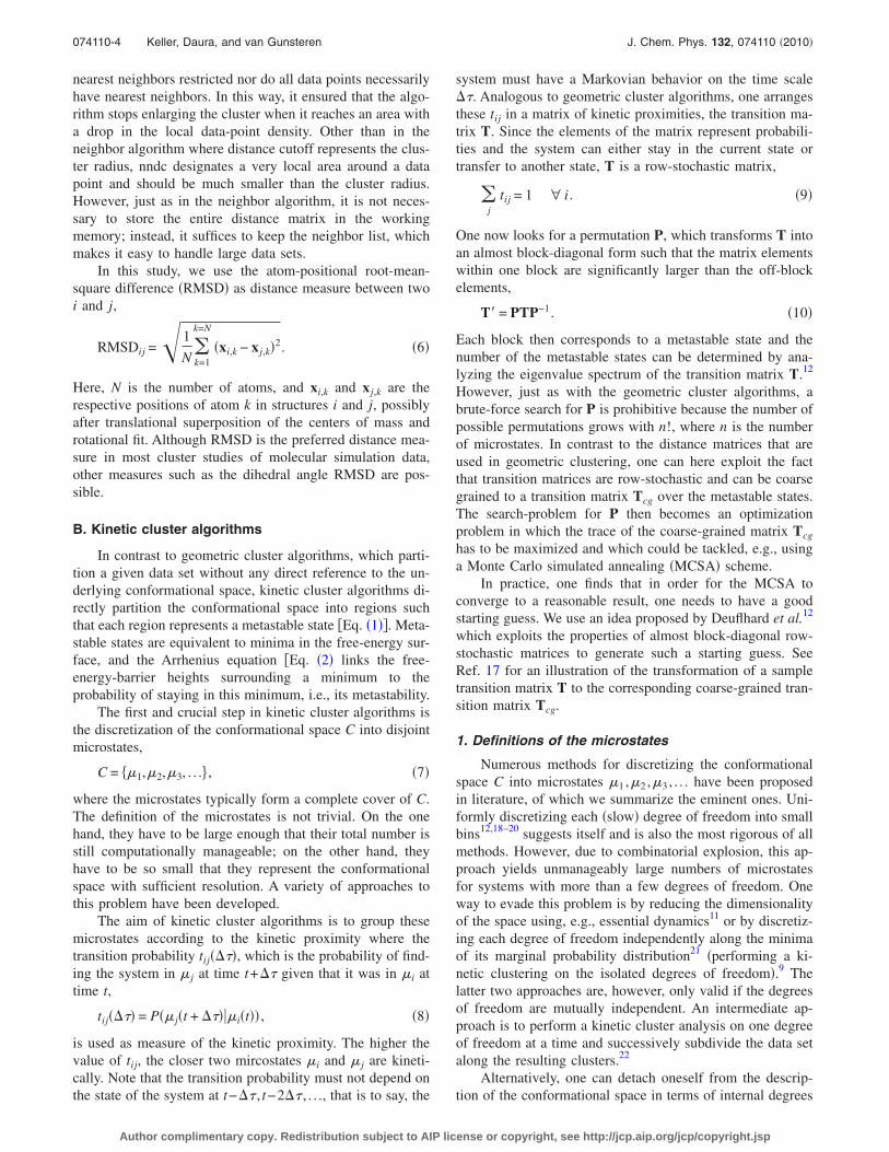
The third algorithm is a close variant of the Jarvis–Patrick algorithm,16 which we—in order to have a more de-scriptive name—will call the common-nearest-neighbor al-gorithm. In contrast to most geometric cluster algorithms,this algorithm is not based on the idea that members of acluster are closer to each other than to all other data points inthe data set, and it therefore also abandons the notion thatclustering is equivalent to reorganizing the distance matrixinto a block-diagonal form. Instead, it bases its cluster defi-nition on a measure for the local data-point density around apoint i which mimics the way we �as human beings� intu-itively recognize clusters in data sets such as, e.g., the scat-terplots in Fig. 1. For this intuitive perception, neither thedistance of a given data point from the cluster center nor thespecific shape of the cluster—parameters that are utilized inmany geometric cluster algorithms—plays a crucial role. Noris the condition that intracluster distances should be smaller

than intercluster distances always fulfilled �see Fig. 1, testcases 3–5�. Rather, we perceive the clusters as continuousareas of high data point density and the cluster boundariesare designated by a steep drop in data point density. In thecommon-nearest-neighbor algorithm, a hitherto unassigneddata point is added to a cluster if it is connected to one of itsmembers by an area of sufficiently high data-point density. Acluster is complete and is removed from the data pool if nofurther data point can be added. Since the data-point densitybetween two data points i and j is hard to calculate if i and jare points in a high-dimensional space, it is instead estimatedas the number of their common nearest neighbors. The near-est neighbors of i are those data points that lie within thenearest-neighbor-distance cutoff �nndc�. The number ofcommon-nearest neighbors of i and j is the number of datapoints that are both nearest neighbors of i and of j. �Thisnumber is, of course, 0 if i and j are further apart than2nndc.� Suppose i is a member of cluster c1 and j is stillunassigned, then j will become a member of c1 if it has atleast nearest-neighbor-number cutoff �nnnc� neighbors with ior any other member of c1. Once it is assigned to c1, it canalso attract unassigned data points. In contrast to the originalformulation of the Jarvis–Patrick algorithm, in which the ndata points closest to i are considered to be neighbors of iindependent of their distance to i, in the common-nearest-neighbor algorithm only data points that lie within nndc areconsidered to be neighbors. Neither is the total number of

FIG. 1. Results of three geometrical cluster algorithms-neighbor algorithm�column 1�, K-medoids algorithm �column 2�, common-nearest-neighbor al-gorithm �column 3� for five 2D test cases �rows 1–5�. Data points of thesame color belong to one cluster. For the K-medoids algorithm, the clustercenters are indicated as differently colored dots at the center of each cluster.

074110-3 Comparing cluster algorithms for MD data J. Chem. Phys. 132, 074110 �2010�


nearest neighbors restricted nor do all data points necessarilyhave nearest neighbors. In this way, it ensured that the algo-rithm stops enlarging the cluster when it reaches an area witha drop in the local data-point density. Other than in theneighbor algorithm where distance cutoff represents the clus-ter radius, nndc designates a very local area around a datapoint and should be much smaller than the cluster radius.However, just as in the neighbor algorithm, it is not neces-sary to store the entire distance matrix in the workingmemory; instead, it suffices to keep the neighbor list, whichmakes it easy to handle large data sets.

In this study, we use the atom-positional root-mean-square difference �RMSD� as distance measure between twoi and j,

RMSDij = 1

N�k=1

k=N

�xi,k − x j,k�2. �6�

Here, N is the number of atoms, and xi,k and x j,k are therespective positions of atom k in structures i and j, possiblyafter translational superposition of the centers of mass androtational fit. Although RMSD is the preferred distance mea-sure in most cluster studies of molecular simulation data,other measures such as the dihedral angle RMSD are pos-sible.

B. Kinetic cluster algorithms

In contrast to geometric cluster algorithms, which parti-tion a given data set without any direct reference to the un-derlying conformational space, kinetic cluster algorithms di-rectly partition the conformational space into regions suchthat each region represents a metastable state �Eq. �1��. Meta-stable states are equivalent to minima in the free-energy sur-face, and the Arrhenius equation �Eq. �2� links the free-energy-barrier heights surrounding a minimum to theprobability of staying in this minimum, i.e., its metastability.

The first and crucial step in kinetic cluster algorithms isthe discretization of the conformational space C into disjointmicrostates,

C = ��1,�2,�3, . . . , �7�

where the microstates typically form a complete cover of C.The definition of the microstates is not trivial. On the onehand, they have to be large enough that their total number isstill computationally manageable; on the other hand, theyhave to be so small that they represent the conformationalspace with sufficient resolution. A variety of approaches tothis problem have been developed.

The aim of kinetic cluster algorithms is to group thesemicrostates according to the kinetic proximity where thetransition probability tij��, which is the probability of find-ing the system in � j at time t+�� given that it was in �i attime t,

tij�� = P�� j�t + ��i�t�� , �8�

is used as measure of the kinetic proximity. The higher thevalue of tij, the closer two mircostates �i and � j are kineti-cally. Note that the transition probability must not depend onthe state of the system at t−�� , t−2�� , . . ., that is to say, the

system must have a Markovian behavior on the time scale��. Analogous to geometric cluster algorithms, one arrangesthese tij in a matrix of kinetic proximities, the transition ma-trix T. Since the elements of the matrix represent probabili-ties and the system can either stay in the current state ortransfer to another state, T is a row-stochastic matrix,

�j

tij = 1 ∀ i . �9�

One now looks for a permutation P, which transforms T intoan almost block-diagonal form such that the matrix elementswithin one block are significantly larger than the off-blockelements,

T� = PTP−1. �10�

Each block then corresponds to a metastable state and thenumber of the metastable states can be determined by ana-lyzing the eigenvalue spectrum of the transition matrix T.12

However, just as with the geometric cluster algorithms, abrute-force search for P is prohibitive because the number ofpossible permutations grows with n!, where n is the numberof microstates. In contrast to the distance matrices that areused in geometric clustering, one can here exploit the factthat transition matrices are row-stochastic and can be coarsegrained to a transition matrix Tcg over the metastable states.The search-problem for P then becomes an optimizationproblem in which the trace of the coarse-grained matrix Tcg

has to be maximized and which could be tackled, e.g., usinga Monte Carlo simulated annealing �MCSA� scheme.

In practice, one finds that in order for the MCSA toconverge to a reasonable result, one needs to have a goodstarting guess. We use an idea proposed by Deuflhard et al.12

which exploits the properties of almost block-diagonal row-stochastic matrices to generate such a starting guess. SeeRef. 17 for an illustration of the transformation of a sampletransition matrix T to the corresponding coarse-grained tran-sition matrix Tcg.

1. Definitions of the microstates

Numerous methods for discretizing the conformationalspace C into microstates �1 ,�2 ,�3 , . . . have been proposedin literature, of which we summarize the eminent ones. Uni-formly discretizing each �slow� degree of freedom into smallbins12,18–20 suggests itself and is also the most rigorous of allmethods. However, due to combinatorial explosion, this ap-proach yields unmanageably large numbers of microstatesfor systems with more than a few degrees of freedom. Oneway to evade this problem is by reducing the dimensionalityof the space using, e.g., essential dynamics11 or by discretiz-ing each degree of freedom independently along the minimaof its marginal probability distribution21 �performing a ki-netic clustering on the isolated degrees of freedom�.9 Thelatter two approaches are, however, only valid if the degreesof freedom are mutually independent. An intermediate ap-proach is to perform a kinetic cluster analysis on one degreeof freedom at a time and successively subdivide the data setalong the resulting clusters.22

Alternatively, one can detach oneself from the descrip-tion of the conformational space in terms of internal degrees



of freedom and instead regard the conformations of the mol-ecule as a whole, e.g., by performing a geometric clusteranalysis which is then iteratively refined using kineticclustering8 or by projecting the configuration of a proteinonto a binary code in which each digit represents one aminoacid and denotes whether this amino acid is in a helical stateor not �encoded as 1 and 0, respectively�.23 In another ver-sion of these secondary structure strings, multiple secondarystates are encoded as letters and the configuration of the pro-tein is represented by a letter string.10

2. Generation of the transition matrix

Once one has decided on a definition of the microstates,each structure q�t� from a trajectory of molecular structuresis projected onto the appropriate microstate �= f�q�t��,thereby transforming this trajectory into a trajectory of mi-crostates

�q�0�,q�t1�,q�t2�, . . .� → ��0�,��t1�,��t2�, . . .� . �11�

It is now possible to count the transitions �i→� j that occurwithin a lag time of t=��.

By moving a frame of t=�� over a MD trajectory, oneobtains the number of transitions f ij between microstate �i

and microstate � j which can be arranged into a so-calledfrequency matrix F. Normalizing the rows of F, one obtainsthe transition matrix T whose elements tij represent the prob-ability of moving from microstate �i to microstate � j withintime t=��.

3. Markovian behavior

The description of the kinetics of a molecules in terms ofa transition matrix is only valid if the kinetics are Markovianon the chosen time scale ��. Given that the system is inmicrostate �i at time t, the probability that it will be in � j att+�� must not depend on the previous states of the systembut only on a time-invariant transition probability tij,

tij = P��t + �� = � j��t� = �i� . �12�

Analyzing the eigenvalues i�� of transition matrices withvarying lag times � of a given system is an elegant way totest whether the dynamics of the systems is Markovian.24

The quantity

�c,i = −�

ln i��13�

is a characteristic time scale for the decay of the eigenvaluei�� with increasing lag time �. If the transition matricesdescribe the dynamics of a Markovian system, this time scaleshould be a constant and plotting �c,i versus � should result ina horizontal line.

III. METHODS

A. Simulation

Twenty production runs of the �-heptapeptideH-�-HVal-�-HAla-�-HLeu-�S ,S�- � -HAla��Me� - �-HVal-�-HAla-�-HLeu-OH �see Fig. 2� in methanol were gener-ated. The starting structures for each of the replicas were

taken randomly from a previous simulation25 of 400 ns. Eachof the replicas was simulated for 500 ns, adding up to a totalof 10 �s of the simulation data. The simulations were car-ried out with the GROMOS96 software26 and the GROMOS43A1 force field26 as previously.25 All bond lengths wereconstrained using the SHAKE algorithm,27 allowing for atime step of 2 fs. Solute configurations were saved every0.1 ps. The system was simulated in a rectangular box usingperiodic boundary conditions. The volume was kept con-stant, and the solvent and solute molecules were indepen-dently weakly coupled to temperature baths of 310 K �Ref.28� with a coupling time of 0.1 ps. The number of solventmolecules was 962. We used 0.8 nm/1.4 nm as twin-rangecutoff and 1.4 nm as reaction field cutoff with rf=1.0. Theatom pair list for short-range interactions and theintermediate-range forces were updated every 5 steps.

B. Geometric cluster algorithms

We extracted structures at intervals of 0.1 ns from thesimulations �5000 structures per replica�. 0.1 ns is the timestep for which the system starts to behave Markovian �cf.Sec. III C 2� and the structures that are separated by this timeinterval can be regarded as uncorrelated. For thesestructures—after a translational superposition and rotationalfit—distance matrices were calculated using three differentdistance measures:

�1� atom-positional RMSD of all atoms �aa�,�2� atom-positional RMSD of all backbone atoms �bb1–7�,

and�3� atom-positional RSMD of the backbone atoms of resi-

dues 2–6 �bb2–6�.

Generally, for molecules comparable in size to our�-heptapeptide, a few thousand structures are accepted to besufficient for a structural cluster analysis. To test whether ourRMSD matrices were indeed converged, we constructedRMSD matrices with different numbers of structures: 5000,10 000, 15 000, 20 000, and 25 000.

We used three different geometric cluster algorithms tocluster these data sets: the neighbor algorithm, theK-medoids algorithm, and the common-nearest-neighbor al-gorithm. We present here the pseudocode of the common-nearest neighbor algorithm because this algorithm differs

A

B C D E F

FIG. 2. Panel �a�: chemical structure of the �-heptapeptide H2-�-HVal-�-HAla-�-HLeu-�S ,S�-�-HAla��Me�-�-HVal-�-HAla-�-HLeu-OH+. Panel�b�: structure of the folded state of this �-heptapeptide. Panels �c�–�e�: ar-bitrarily chosen unfolded structures of this �-heptapeptide.



from the more commonly used K-medoids and neighbor al-gorithms in that it bases its cluster criterion on a local densityestimate. The pseudocode of the two other algorithms can befound in the Appendix.

1. Common-nearest-neighbor-cluster algorithm

The common-nearest-neighbor-cluster algorithm has twoinput parameters—the nearest-neighbor-distance cutoff nnncand the nearst-neighbor-number cutoff nncc—and is com-posed of the following steps:

�1� Loop over all data points that have not been assigned toa cluster yet.

• Find the data point with the highest number of nearestneighbors within the nndc.

�2� This data point is the medoid of the current cluster.�3� Loop over all data points that have not been assigned to

a cluster yet and keep looping until no further datapoint can be added to the current cluster.

• For each data point, check if its number of common-nearest neighbors with any of the points that have beenassigned to the current cluster so far is equal to orgreater than the nnnc.

• If this is true, add this data point to the current cluster.

�4� Add the current cluster to the list of clusters and re-move its members from the pool of unassigned datapoints.

�5� Repeat steps �1�–�4� until all data points have been as-signed to a cluster.

C. Kinetic cluster algorithms

1. Definition of the microstates and generationof the transition matrix

Two approaches are possible for the definition of mi-crostates: �i� sorting the structure of the trajectory into verysmall clusters using a geometric cluster algorithm or �ii� dis-cretizing the conformational space �or subspace of the con-formational space� directly. With regard to a comparisonwith the results of geometric cluster algorithms, the formerapproach has the advantage that one could use the same met-ric for geometric and kinetic clustering, but the disadvantagethat a microstate definition which relies on a geometric clus-ter algorithm is likely to bias the comparison. Also note thatthe concept of metastable states exists, independent of the

representation of the molecule and as long as the chosenmetric does not obscure the barriers in the system, kineticclustering should reliably yield the metastable states. Wetherefore opted for the latter approach.

We discretized the three possible backbone torsionalangles of residue i, C�O�i−1–Ni–C�,i–C�,i, theNi–C�,i–C�,i–C�O�i, and the C�,i–C�,i–C�O�i–Ni+1 dihe-dral angles of residues 2–6 following a procedure describedin Ref. 9. In this approach one checks whether the torsionalangles are mutually independent and, if so, performs a ki-netic cluster analysis on each torsional angle separatelythereby discretizing this degree of freedom into a small num-ber of bins. The possible microstates of the molecule are thena combination of these bins. The C�,i–C�O�i–Ni+1–C�,i+1

dihedral angle does not need to be discretized because it isthe dihedral angle of the peptide plane which is restrained toa planar conformation. This yielded two dihedral angle mi-crostates for each C�O�i−1–Ni–C�,i–C�,i dihedral angle,three microstates for each Ni–C�,i–C�,i–C�O�i dihedralangle and four �residues 3, 5, and 6� �two �residues 2 and 4��for the C�,i–C�,i–C�O�i–Ni+1 dihedral angles. The exactboundaries of these dihedral angle microstates are given inTable I. A microstate of the overall peptide conformation isconstructed as a combination of dihedral angle microstates.With the given discretization this amounts to a total of1 990 656 possible microstates, most of which are, however,never visited during the simulation. In order to decide whichof all these possible microstates should be taken into accountfor the construction of the transition matrix, we counted howoften each of the possible microstates was visited during the10 �s of simulation and discarded those microstates thatwere visited by less then 0.01% of all trajectory structures.This yielded a total of 87 microstates for which we con-structed transition matrices with lag times ranging from �=10 ps to �=500 ps. Transitions from and to the discardedmicrostates were not included in the construction of the tran-sition matrices and detailed balance was enforced by readingout the trajectories forward and backward, i.e., each transi-tion from a microstate i to a microstate j was also counted asa transition from j to i. From a test set of 15 000 structures,11 942 fall within these 87 microstates and 3058 structuresoccupy one of the discarded microstates and were classifiedas unstructured data �cf. line 2 in Table 8�.

2. Identification of the metastable states

We checked whether the dynamics of the �-heptapeptidecan be described as a Markov process using Eq. �13�. For lagtimes � greater than 100 ps, the characteristic time scales for

TABLE I. Microstate boundaries of the flexible backbone torsional angles of residues 2–6 in the �-heptapeptide. Values are in degrees. The cis-conformationcorresponds to 0°.

Residue No. Residue name C�O�i−1–Ni–C�,i–C�,i Ni–C�,i–C�,i–C�O�i C�,i–C�,i–C�O�i–Ni+1

2 �-HAla 0; 115 0; 120; 240 0; 1903 �-HLeu 0; 135 0; 120; 240 90; 180; 240; 3304 �S ,S�-�HAla��Me� 0; 125 0; 110; 240 0; 1455 �-HVal 0; 120 0; 105; 240 0; 115; 180; 2406 �-HAla 0; 130 0; 115; 240 0; 115; 185; 245



the largest eigenvalues become approximately constant andwe chose the transition matrix with �=300 ps for the iden-tification of the metastable states. A plot of the eigenvalues i

of T��=300 ps� yielded a gap between the fifth and sixtheigenvalues. We can therefore expect to find five metastablestates.12 After having generated a starting guess for the defi-nition of these five metastable states using an idea by Deu-flhard et al.,12 we optimized the state definition by maximiz-ing the trace of the coarse-grained transition matrix �see Eq.�10� and Eqs. �A1�–�A3� in Ref. 17� using the MCSAscheme.8 We started the MCSA at a temperature of TMCSA

=0.006 and decreased it to 0.0001 in 60 steps, making 1000trial moves at each temperature. A trial move consisted ofrandomly picking a microstate within a randomly chosenmetastable state and assigning it to another metastable statewhich was also chosen randomly. If the trace of the resultingcoarse-grained matrix was greater than or equal to the traceof the current coarse-grained matrix, we always accepted it.If it was smaller, we accepted it with a probability of

p = exp��Tr/T� �14�

where �Tr is the difference in the traces of two matrices andT is the current temperature.

Merging two metastable states often leads to a localmaximum of the trace in which the algorithm gets trapped.For this reason, we prohibited empty metastable states, i.e., ifa metastable state at some point in the optimization consistedof only one microstate, then this microstate could not bechosen for a trial move. Note, however, that if a system withn metastable states is described by a transition matrix withless than n states �merged metastable states�, the trace of thismatrix lies below the optimal trace. Therefore, the mergingof metastable states during the optimization is an indicationthat the starting guess or temperature or the temperaturesteps of the MCSA scheme were not chosen appropriately.We repeated the algorithm 80 times and used the definitionof the metastable states that corresponded to the coarse-grained matrix with the largest trace.

IV. RESULTS

A. Test cases

Two-dimensional �2D� data sets, such as the five testcases in Fig. 1, are particularly useful when characterizinggeometric cluster algorithms because in contrast to high-dimensional data sets the results can be directly representedin terms of 2D scatterplots, thereby revealing the featuresand peculiarities of the cluster algorithm. Note that although

the cluster algorithms might show a more complex behaviorfor higher-dimensional data sets, flaws which were detectedfor the 2D test cases will definitely also affect the resultswhen the algorithms are applied to high-dimensional datasets such as molecular simulation data.

We clustered each of the test cases with all three geo-metric cluster algorithms �neighbor algorithm, K-medoids al-gorithm, and common-nearest-neighbor algorithm� and alsosystematically varied the input parameters. By visual inspec-tion of the resulting 2D scatterplots, we decided whether thetest sets had been clustered correctly, i.e., according to hu-man intuition. In the following, we will refer to those groupsof data points that are recognized as clusters by the humanintuition as “data point heap,” whereas the word “cluster”will denote the results of the respective cluster algorithms.

All three geometric cluster algorithms succeed in clus-tering test cases 1 and 2. For test case 3, the K-medoids andthe common-nearest-neighbor algorithms converge to a cor-rect solution, whereas for test cases with concave clusters�test cases 4 and 5�, only the common-nearest neighbor al-gorithm partitions the data set correctly. Note, however, thatthe results of the K-medoids algorithm depend not only onthe input parameter k �number of clusters� but also on theinitialization �first assignment of data points to clusters�, thatis, different runs with the same value of k can and will leadto different partitions of the data set. Such a situation arosefor test case 2 with k=5 and test case 3 with k=2. �All othervalues of k led to wrong partitions of the two data sets.� Thecommon-nearest-neighbor algorithm is the only algorithmthat partitions all five test cases correctly. It is also robustwith respect to a variation in its two input parameters: nndcand nnnc. Table II illustrates this: independent of the testcase, we can vary nndc largely and find at least one value ofthe nnnc for which the data set is clustered correctly.

Figure 1 also highlights the peculiarities and deficienciesof each of the algorithms. In the neighbor algorithm, the datapoint which has the most neighbors within a certain cutoffradius is considered the center of the next cluster. Once thiscluster center is set, no correction is possible and all neigh-boring data points are assigned to this cluster. If two data-point heaps are not well separated or if their distance issmaller than the respective elongation �as in test case 3�, thecluster center can very well be assigned to a data point thatlies in between the two data point heaps and the resultingcluster will comprise data points from both. The characteris-tic structure of this “cutting effect” is a large circular cluster,such as the black cluster in panel �7� of Fig. 1, the borders ofwhich do not correspond to the limits of the data-point heaps.

TABLE II. Combinations of nndc and nnnc for which test cases 1–5 were clustered correctly by the nearest-common-neighbor algorithm and the resultingnumber of large clusters ��5 members�, small clusters �1–5 members�, and the total number of clusters.

Test case 1 Test case 2 Test case 3 Test case 4 Test case 5

nndc 2 3 4 5 2 3 4 5 2 3 4 5 2 3 4 5 2 3 4 5nnnc 2 6 11 20 2 3 10 13 2 5 11 ¯ 2 4 5 14 ¯ 2 4 13

Large 2 2 2 2 5 5 5 5 2 2 2 ¯ 2 2 2 2 ¯ 2 2 2Small 5 7 8 13 7 0 12 6 3 3 5 ¯ 0 0 0 3 ¯ 0 1 6Total 7 9 10 15 12 5 17 11 5 5 7 ¯ 2 2 2 5 ¯ 2 3 8



Panel �5� in the same figure shows a result of the K-medoidsalgorithm for the second test case. This algorithm starts byrandomly choosing k cluster centers from the data set andthen iteratively optimizes cluster memberships and clustercenters until convergence. Convergence is usually reachedafter a few iterations. The algorithm, however, does not al-ways converge to the intuitive result. Often we see results inwhich a large data-point heap is split into two or more parts,such as the central data-point heap in panel �5� of Fig. 1, orsmall data-point heaps are merged into one cluster, such asthe two data-point heaps on the left side of the same panel.This typically happens when during the initialization twocluster centers are assigned to data points which are in thesame �large� data-point heap. If the data-point density moreor less steadily decreases from the center of the data-pointheap to its rims, such as in the first test case we often see thatdata points at the rim of the heap are split off as singletons�dots with various colors in panel �3� of Fig. 1�. This effect isnot severe for a 2D data set as only a few data points are splitoff, but for higher-dimensional data sets, the ratio betweenthe number of data points on the rim of a data-point heap andthose at the center increases, which makes this effect pro-nounced.

B. Geometric clustering results for a �-heptapeptide

1. Structural RMSD value distributions

In geometric cluster analysis, the RMSD matrix has tomeet two conditions in order to be a faithful representationof the conformational ensemble of the molecule under study:�i� the structures that were used for the construction of thematrix have to be uncorrelated and �ii� there have to beenough structures to cover the entire conformational spacewith correct weights. We satisfy the first condition by onlyusing structures that are separated by 0.1 ns in the trajectoryof the �-heptapeptide �Fig. 2� and we test the second condi-tion by constructing two RMSD matrices with the same pa-rameters �i.e., atom set and number of structures� from inde-pendent simulations and then comparing the distribution ofRMSD values within these matrices. Figure 3 shows the dis-tribution of RMSD matrix elements resulting from using5000 �row 1�, 10 000 �row 2�, 15 000 �row 3�, 20 000 �row4�, and 25 000 �row 5� molecular structures calculated usingthe three different atom sets: aa �column 1�, bb1–7 �column2�, and bb2–6 �column 3�. Each of the graphs shows twoRMSD distributions for which the structures were drawnfrom independent simulations �5000 structures: simulations 1and 10; 10 000 structures: simulations 1, 2, 11, and 12;15 000 structures: simulations 1–3 and 11–13; 20 000 struc-tures: simulations 1–4 and 11–14; and 25 000 structures:simulations 1–5 and 11–15�. For 5000 structures, the generalfeatures of the RMSD distributions, i.e., number and positionof the peaks, are similar for each of the atom sets. However,the relative weights of the peaks differ greatly for RMSDmatrices that were constructed from different simulations,indicating that the various parts of conformational spacehave not yet been sampled with equilibrium weights. Thetwo distributions become more similar as we add more struc-tures, but even for 25 000 structures complete agreement is

not achieved. Since the similarity of the two distributionsdoes not significantly improve beyond 15 000 structures, wedecided to use RMSD matrices with 15 000 structures forgeometric clustering in this study. The fact that the twoRMSD distributions have approximately the same shape isnot a sufficient proof that the conformational space has beensampled completely. Rather, one should regard this as a nec-essary condition or an indication of complete sampling. Inpractice, however, the available simulation data often limitsthe number of structures that can be used for the constructionof RMSD matrices to a few thousand even for considerablylarger systems,15,29 which almost certainly imposes a largeuncertainty in the calculated cluster sizes.

The RMSD distributions of the three different atom setsin Fig. 3 reflect two known effects: �i� the RMSD valuesincrease if more atoms are added to the sets and �ii� if thevery mobile side chains and terminal residues are included inthe atom set, their large displacements dominate the RMSDvalues leading to a less structured RMSD distribution.

2. Choice of cluster parameters

The question of how to choose appropriate cluster pa-rameters has to be answered differently for each of the algo-rithms. For the neighbor-cluster algorithm, the distance cut-off c represents the radius of a “typical” cluster within agiven data set and can be estimated in two ways.

0.0 0.4 0.8

01234

RMSD / nm

p[1

/nm

] 1

0.0 0.4 0.8

01234

RMSD / nm

p[1

/nm

] 4

0.0 0.4 0.8

01234

RMSD / nm

p[1

/nm

] 7

0.0 0.4 0.8

01234

RMSD / nm

p[1

/nm

] 10

0.0 0.4 0.8

01234

RMSD / nm

p[1

/nm

] 13

0.0 0.4 0.8

01234

RMSD / nm

p[1

/nm

] 2

0.0 0.4 0.8

01234

RMSD / nm

p[1

/nm

] 5

0.0 0.4 0.8

01234

RMSD / nm

p[1

/nm

] 8

0.0 0.4 0.8

01234

RMSD / nm

p[1

/nm

] 11

0.0 0.4 0.8

01234

RMSD / nm

p[1

/nm

] 14

0.0 0.2 0.4 0.6

02468

RMSD / nm

p[1

/nm

] 3

0.0 0.2 0.4 0.6

02468

RMSD / nm

p[1

/nm

] 6

0.0 0.2 0.4 0.6

02468

RMSD / nm

p[1

/nm

] 9

0.0 0.2 0.4 0.6

02468

RMSD / nm

p[1

/nm

] 12

0.0 0.2 0.4 0.6

02468

RMSD / nm

p[1

/nm

] 15

all atoms backbone atomsresidues 1−7

backbone atomsresidues 2−6

5000structures

10000structures

15000structures

20000structures

25000structures

FIG. 3. Distribution of RMSD values in RMSD matrices of 5000 data points�row 1�, 10 000 data points �row 2�, 15 000 data points �row 3�, 20 000 datapoints �row 4�, 25 000 data points �row 5� calculated using different atomsets: aa �column 1�, bb1–7 �column 2�, bb2–6 �column 3�, and data from 11different 500 ns simulations of the �-heptapeptide; solid line: data pointsdrawn from simulations 1 �row 1�, 1 and 2, �row 2�, 1–3 �row 3�, 1–4 �row4�, and 1–5 �row 5�; dotted line: data points drawn from simulations 10 �row1�, 11 and 12, �row 2�, 11–13 �row 3�, 11–14 �row 4�, and 11–15 �row 5�.



• The time series of the RMSD to the folded �NMR or xray� structure shows, for a folding-unfolding equilib-rium such as exhibited by �-heptapeptides, a gap be-tween folded and unfolded structures. RMSD valuesthat lie in this gap are a good estimate for radius of thefolded state and can be used as a distance cutoff.

• The first minimum in the RMSD distribution �see Fig.3� is an equally good estimate for this radius �and hencefor the distance cutoff� and can be determined moreprecisely.

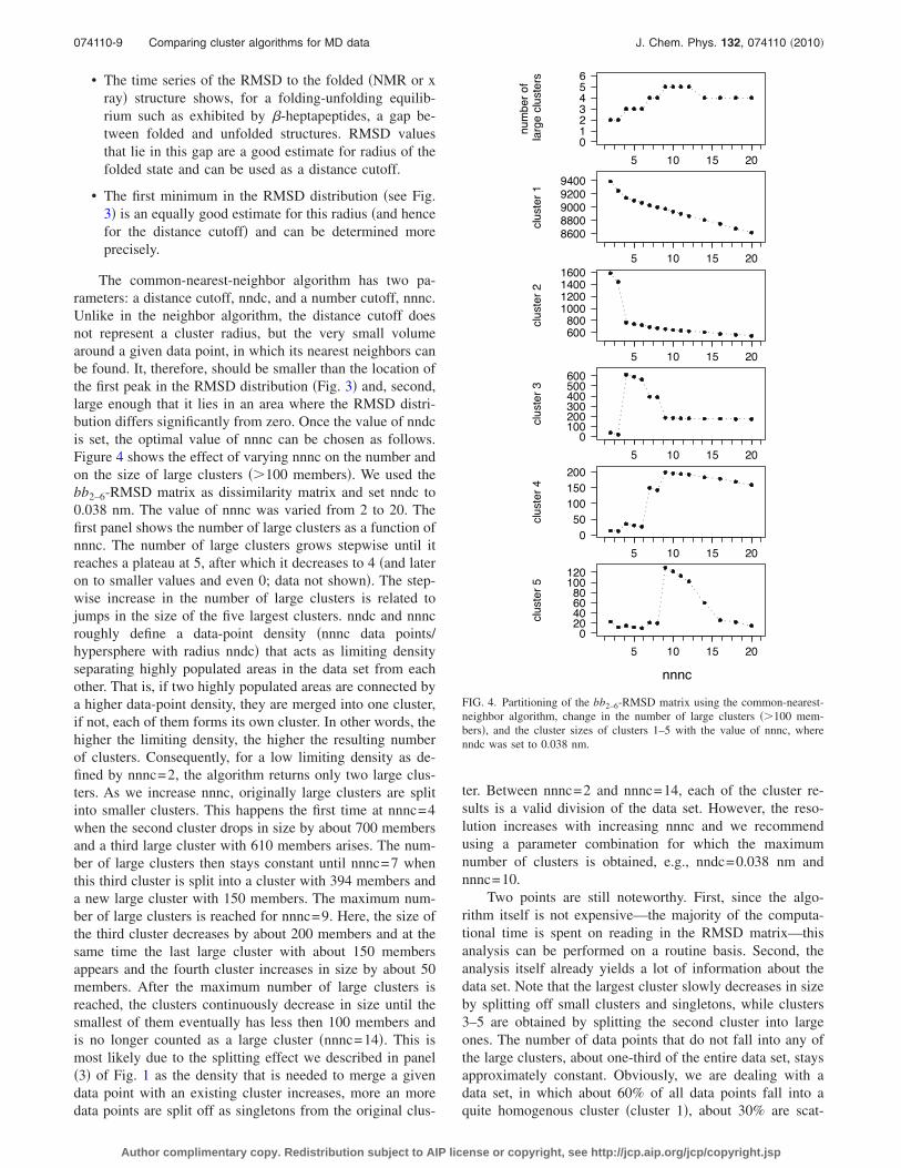
The common-nearest-neighbor algorithm has two pa-rameters: a distance cutoff, nndc, and a number cutoff, nnnc.Unlike in the neighbor algorithm, the distance cutoff doesnot represent a cluster radius, but the very small volumearound a given data point, in which its nearest neighbors canbe found. It, therefore, should be smaller than the location ofthe first peak in the RMSD distribution �Fig. 3� and, second,large enough that it lies in an area where the RMSD distri-bution differs significantly from zero. Once the value of nndcis set, the optimal value of nnnc can be chosen as follows.Figure 4 shows the effect of varying nnnc on the number andon the size of large clusters ��100 members�. We used thebb2–6-RMSD matrix as dissimilarity matrix and set nndc to0.038 nm. The value of nnnc was varied from 2 to 20. Thefirst panel shows the number of large clusters as a function ofnnnc. The number of large clusters grows stepwise until itreaches a plateau at 5, after which it decreases to 4 �and lateron to smaller values and even 0; data not shown�. The step-wise increase in the number of large clusters is related tojumps in the size of the five largest clusters. nndc and nnncroughly define a data-point density �nnnc data points/hypersphere with radius nndc� that acts as limiting densityseparating highly populated areas in the data set from eachother. That is, if two highly populated areas are connected bya higher data-point density, they are merged into one cluster,if not, each of them forms its own cluster. In other words, thehigher the limiting density, the higher the resulting numberof clusters. Consequently, for a low limiting density as de-fined by nnnc=2, the algorithm returns only two large clus-ters. As we increase nnnc, originally large clusters are splitinto smaller clusters. This happens the first time at nnnc=4when the second cluster drops in size by about 700 membersand a third large cluster with 610 members arises. The num-ber of large clusters then stays constant until nnnc=7 whenthis third cluster is split into a cluster with 394 members anda new large cluster with 150 members. The maximum num-ber of large clusters is reached for nnnc=9. Here, the size ofthe third cluster decreases by about 200 members and at thesame time the last large cluster with about 150 membersappears and the fourth cluster increases in size by about 50members. After the maximum number of large clusters isreached, the clusters continuously decrease in size until thesmallest of them eventually has less then 100 members andis no longer counted as a large cluster �nnnc=14�. This ismost likely due to the splitting effect we described in panel�3� of Fig. 1 as the density that is needed to merge a givendata point with an existing cluster increases, more an moredata points are split off as singletons from the original clus-

ter. Between nnnc=2 and nnnc=14, each of the cluster re-sults is a valid division of the data set. However, the reso-lution increases with increasing nnnc and we recommendusing a parameter combination for which the maximumnumber of clusters is obtained, e.g., nndc=0.038 nm andnnnc=10.

Two points are still noteworthy. First, since the algo-rithm itself is not expensive—the majority of the computa-tional time is spent on reading in the RMSD matrix—thisanalysis can be performed on a routine basis. Second, theanalysis itself already yields a lot of information about thedata set. Note that the largest cluster slowly decreases in sizeby splitting off small clusters and singletons, while clusters3–5 are obtained by splitting the second cluster into largeones. The number of data points that do not fall into any ofthe large clusters, about one-third of the entire data set, staysapproximately constant. Obviously, we are dealing with adata set, in which about 60% of all data points fall into aquite homogenous cluster �cluster 1�, about 30% are scat-

FIG. 4. Partitioning of the bb2–6-RMSD matrix using the common-nearest-neighbor algorithm, change in the number of large clusters ��100 mem-bers�, and the cluster sizes of clusters 1–5 with the value of nnnc, wherenndc was set to 0.038 nm.



tered around the conformational space without forming clus-ters �unstructured data�, and the remaining 10% are spreadamong 4 large clusters.

The K-medoids-cluster algorithm takes the number ofclusters as an input parameter. Unfortunately, usually nothingis known about the optimal number of clusters unless onealready has results from other cluster algorithms. Since boththe neighbor-cluster and the common-nearest-neighbor-cluster algorithms indicated that there are only few dominantclusters, we varied the input parameter from k=2 to k=9 insteps of 1 �data not shown� and present results for k=5 in theremainder of this publication.

3. Cluster sizes

We clustered RMSD matrices that were constructed forthree different atom sets �aa, bb1–7, and bb2–6� using threedifferent geometric cluster algorithms. For each combinationof RMSD matrix and cluster algorithm, we conducted theanalysis three times with slightly varied input parameters.

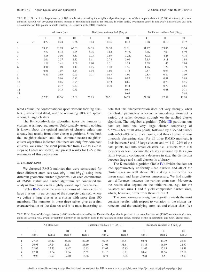
Tables III–V show the results in terms of cluster sizes oflarge clusters �in percentage of the complete data set�, wherewe define a large cluster as a cluster with more than 100members. The numbers in these three tables give us a firstcharacterization of the data set and it is most interesting to

note that this characterization does not vary strongly whenthe cluster parameters or even the underlying atom set isvaried, but rather depends strongly on the applied clusteralgorithm. The neighbor algorithm �Table III� partitions ourdata set into one very large cluster comprising of�52%–66% of all data points, followed by a second clusterwith �6%–9% of all data points, and then clusters of con-tinuously decreasing size. For all three RMSD matrices, itfinds between 8 and 13 large clusters and �11%–27% of thedata points fall into small clusters, i.e., clusters with 100members or less. Because the clusters returned by this algo-rithm typically continuously decrease in size, the distinctionbetween large and small clusters is arbitrary.

The K-medoids algorithm �Table IV� divides the data setinto approximately uniformly sized clusters and all of thecluster sizes are well above 100, making a distinction be-tween small and large clusters unnecessary. We find signifi-cant differences between the various atom sets. Moreover,the results also depend on the initialization, e.g., for theaa-atom set, runs 1 and 2 yield comparable cluster sizes,which, however, differ from those of run 3.

The common-nearest-neighbor algorithm yields the mostconstant results, with respect to variation in the cluster pa-rameters and the underlying atom set and cluster sizes �see

TABLE III. Sizes of the large clusters ��100 members� returned by the neighbor algorithm in percent of the complete data set �15 000 structures�: first row,atom set; second row ,n=cluster number, number of the partition used in the text, and in other tables, c=distance cutoff in nm; body, cluster sizes; last row,s.c.=number of data points in small clusters, i.e., clusters with �100 members.

n

All atom �aa� Backbone residues 1–7 �bb1–7� Backbone residues 2–6 �bb2–6�

I II III I II III I II IIIc 0.22 0.24 0.26 0.14 0.16 0.18 0.08 0.10 0.12

1 59.53 61.99 65.63 54.35 58.30 61.2 51.77 59.85 63.542 7.72 8.33 7.25 6.75 7.63 9.127 6.46 7.03 8.993 4.15 3.06 3.53 3.73 3.89 3.247 5.02 4.25 4.784 2.06 2.37 2.32 3.11 2.78 3.06 3.15 3.11 1.985 1.18 1.41 1.68 1.90 1.31 1.29 2.69 1.43 1.846 0.91 1.09 1.47 1.15 1.10 1.26 1.46 1.29 1.197 0.91 1.07 1.14 1.04 1.05 1.12 0.87 0.93 1.198 0.85 0.93 0.93 0.71 0.87 1.00 0.83 0.89 1.099 0.86 0.83 0.86 0.87 0.75 0.81 0.9910 0.85 0.75 0.73 0.86 0.78 0.9511 0.77 0.73 0.70 0.74 0.70 0.8512 0.73 0.73 0.69 0.68 0.7113 0.69 0.68s.c. 22.70 16.56 13.01 27.25 20.7 14.78 27.00 17.57 11.20

TABLE IV. Sizes of the large clusters ��100 members� returned by the K-medoids algorithm in percent of the complete data set �15 000 structures�: first row,atom set; second row, n=cluster number, number of the partition used in the text and in other tables, number of the initialization; and body, cluster sizes.

n


I II III I II III I II IIIRun 1 Run 2 Run 3 Run 1 Run 2 Run 3 Run 1 Run 2 Run 3

1 27.56 27.42 26.06 27.70 46.45 34.81 50.71 49.39 29.592 26.93 27.24 20.11 26.69 21.01 31.61 18.15 16.99 22.373 22.63 22.73 18.47 16.93 12.67 15.83 11.03 15.15 18.414 12.91 11.64 17.96 15.32 11.16 9.71 10.69 11.96 17.605 9.98 10.97 17.40 13.36 8.71 8.05 9.41 6.51 12.03



Table V�. Similar to the neighbor algorithm, it finds one largecluster covering �53%–60% of the data points, all otherclusters are smaller by at least an order of magnitude withthe second cluster covering about 4%–5% of the data points.The algorithm finds between 3 and 5 large clusters and sorts�31%–40% of the data points into small clusters. Contraryto the neighbor algorithm, the 100-member-limit marks a gapin the cluster sizes inherent to this algorithm: large clustersare well above this limit and the vast majority of the smallclusters are singletons with only few small clusters compris-ing of 5–30 members.

4. Variation in the cluster parameters and theunderlying atom set

When comparing two alternative partitions A= �a1 ,a2 , . . . and B= �b1 ,b2 , . . . of a given data set, similarcluster sizes are only a hint that these two partitions might besimilar, but do not constitute a sufficient proof. To assesshow similar the two partitions are, one needs to know howlarge the overlap between any pair of clusters ai ,bj is, i.e.,how many of the data points in ai are also found in bj. InTables VI and VII we report this type of overlap numbers forvarious partitions of our data set. We consider only the fivelargest clusters of each partition and again sort them by sizeand arrange the overlap numbers in a matrix �three matricesper panel�. If two partitions are very similar, one would ex-pect numbers in the order of the corresponding cluster sizeson the diagonal elements and mostly zeros or small entries inthe off diagonal elements. Conversely, if two partitions arevery different, one expects large entries on both the diagonaland off-diagonal elements.

Table VI assesses the influence of a slight variation inthe parameters on the partition of a given data set. Here, weonly report for each algorithm �panels �1�–�3�� the overlapmatrices for different partitions of the bb2–6-RMSD matrix,but the overlap matrices of the other atom sets yield a similarpicture. For each of the three distance cutoffs: �I� c=0.08 nm, �II� c=0.10 nm, and �III� c=0.12 nm, the neigh-bor algorithm identifies one dominant cluster, all of whichhave a large overlap with each other. More precisely, the sizeof this first cluster is directly linked to the distance cutoff c:the relatively small cluster of I is a subset of cluster 1 in II as

well as in III. Likewise, cluster 1 in II is a subset cluster 1 inIII. Apart from that, clear matches between clusters of differ-ent partitions are rare. More often one finds that a cluster inone partition is a subset of a larger cluster in another parti-tion, e.g., cluster 3 in I is a subset of both cluster 2 in II andcluster 2 in III.

In the K-medoids algorithm we did not vary the clusterparameter k but rather the initialization and present the re-sults for k=5. Runs 1 �I� and 2 �II� yield similar cluster sizesand also the overlap between the respective clusters 1 and 2is large. Despite the fact that both clusters 1 and 2 in I alsohave overlap with cluster 5 from II, the overlap is so largethat we can safely say that clusters 1 and 2 in I are the sameas clusters 1 and 2 in II. The overlap pattern for clusters 3—5is more complicated and no clear match is possible. Run 3�III� yields cluster sizes that were quite different from thosein I and II, yet we can still match some of its clusters to thepartitions I and II: clusters 1 and 2 in III together constitutecluster 1 in I or II, also cluster 4 in III is largely identical tocluster 2 in I or II. Clusters 3 and 5 cannot be matched. Oneshould, however, also note that these overlaps are not asclear as in the comparison of I and II.

The common-nearest-neighbor algorithm is the most ro-bust of the three geometric cluster algorithms with respect toa variation in the input parameters. Clusters 1, 2, and 4 in I�nndc=0.036 nm, nnnc=4� are largely identical to clusters1, 2, and 5 in II �nndc=0.038 nm, nnnc=10�. In the com-parison of I and III �nndc=0.040 nm, nnnc=10�, againclusters 1 and 2 in I match clusters 1 and 2 in III, whereasclusters 3 and 4 in I together constitute cluster 3 in III. Theoverlap of II and III yields as similar picture: again the re-spective clusters 1 and 2 match and cluster 3 in III is splitinto clusters 3–5 in II.

In Table VII we test the sensitivity of the neighbor algo-rithm and the common-nearest-neighbor algorithm with re-spect to the variation in the underlying atom set. In theneighbor algorithm, the largest clusters for all atom setsshow the largest overlap among each other meaning thatclusters 1 in aa, bb1–7, and bb2–6, respectively, are largelyidentical. Also the second clusters for all three atom sets stillshow about 80% overlap among each other. Clusters 3–5 inaa cannot be clearly matched to any of the clusters in bb1–7

TABLE V. Sizes of the large clusters ��100 members� returned by the common-nearest-neighbor algorithm in percent of the complete data set �15 000structures�: first row, atom set; second row, n=cluster number, number of the partition used in the text and in other tables, nndc=nearest-neighbor-distancecutoff in nm, nnnc=nearest-neighbor-number cutoff; body, cluster sizes; and last row, s.c.=number of data points in small clusters, i.e., clusters with �100members.

n


I II III I II III I II IIInndc 0.09 0.10 0.11 0.06 0.07 0.08 0.036 0.038 0.04nnnc 2 3 6 6 12 20 4 10 10

1 52.92 54.96 56.17 55.25 57.37 59.09 60.43 59.54 60.272 3.51 3.97 4.32 4.07 4.52 4.87 4.83 4.29 4.613 2.30 2.47 2.61 2.39 2.63 2.88 2.74 1.31 3.614 1.25 1.41 1.45 1.39 1.46 1.55 1.17 1.235 0.81s.c. 39.91 37.10 35.22 36.75 33.96 31.61 30.66 32.83 31.37



or bb2–6. The difference between bb1–7 and bb2–6 is smaller:here, also the third clusters are largely identical. Despite thefact that the kernels of the largest clusters were not affected,part of their members was assigned to other clusters whenthe atom set changed. This is reflected by the large off-diagonal elements in the overlap matrices. For example, inthe first row of the overlap matrix between aa and bb2–6, onesees that 119 and 264 members of the largest cluster in aahave been assigned to clusters 2 and 4 in bb2–6, respectively.This shows that the borders of cluster 1 in one atom setmight cut through clusters 2, 3, or 4 in another atom set.

The picture is different for the common-nearest-neighboralgorithm. Here, the cluster definition seems to be hardlyinfluenced by the choice of the atom set. The overlap be-tween two clusters in different partitions is either in the orderof the cluster size or zero. The difference between clustersize and overlap is covered by small clusters �last row andcolumn in each matrix�. One can speculate on the reasonwhy this algorithm is so robust with respect to the variationin the atom set: in principle, it tries to cut along the minimaof the distribution, thereby identifying its maxima, which, inturn, correspond to the minima of the free-energy surface.Due to sampling, one typically does not analyze the distribu-

tion in the complete conformational space but only its pro-jection onto the conformational subspace of the chosen atomset. Minima that are present in the complete distributionmight be blurred or even absent in its projection; however,the converse—minima that are present in the projection butare less pronounced in the complete distribution—is not pos-sible. Therefore, if the atom set bb2–6 suffices to faithfullyrepresent the essential barriers in the free-energy landscape,adding atoms that move over large distances but are essen-tially unhindered, such as side chains or the terminal resi-dues, will not change the cluster results. Using cluster algo-rithms that define clusters based on some distance to acluster center, such as the neighbor or the K-medoids algo-rithms, adding highly mobile atoms may obscure the clusterboundaries. However, note that these algorithms rely on theassumption that all clusters have an approximately sphericalshape and are separated by distances larger than their diam-eter and here a projection can help fulfill these assumptions.

C. Kinetic clustering results for the �-heptapeptide

We have discretized the conformational space of the�-heptapeptide �cf. Fig. 2� into microstates and—using ki-

TABLE VI. Variation in the cluster parameters �the initializations for different partitions of the bb2–6-RMSD matrix�: first row and column of each subtable,cluster number; second row and column in each subtables, cluster size; body of each subtable, overlap matrix of the first five large clusters; and last row andcolumn of each subtable, s.c.=number of data points in small clusters, i.e., clusters with �100 members and their overlap with other clusters. Neighboralgorithm: �I� c=0.08 nm, �II� c=0.10 nm, and �III� c=0.12 nm. K-medoids algorithm: �I� run 1, �II� run 2, and �III� run 3. Common-nearest-neighboralgorithm: �I� nndc=0.036 nm, nnnc=4; �II� nndc=0.038 nm, nnnc=10; and �III� nndc=0.04 nm, nnnc=10.

Neighbor algorithm

II 1 2 3 4 5 s.c. III 1 2 3 4 5 s.c. III 1 2 3 4 5 s.c.I Size 8978 1054 638 467 215 3648 I Size 9531 1348 717 297 276 2831 II Size 9531 1348 717 297 276 2831

1 7765 7765 0 0 0 0 0 1 7765 7765 0 0 0 0 0 1 8978 8976 0 0 0 0 22 969 678 0 0 281 0 10 2 969 942 0 0 0 0 27 2 1054 5 1018 0 0 0 313 753 0 751 0 0 0 2 3 753 0 753 0 0 0 0 3 638 2 61 575 0 0 04 473 0 0 471 0 0 2 4 473 0 12 461 0 0 0 4 467 364 0 4 0 0 995 403 344 0 0 0 0 59 5 403 375 0 0 0 0 28 5 215 0 130 3 0 17 65s.c. 4637 191 303 167 186 215 3579 s.c. 4637 449 583 256 297 276 2776 s.c. 3648 191 139 135 297 17 2634

K-medoids algorithm, k=5II 1 2 3 4 5 s.c. III 1 2 3 4 5 s.c. III 1 2 3 4 5 s.c.

I Size 7408 2548 2273 1794 977 ¯ I Size 4439 3355 2761 2640 1805 ¯ II Size 4439 3355 2761 2640 1805 ¯

1 7607 7396 0 0 0 211 ¯ 1 7607 4341 3253 2 4 7 ¯ 1 7408 4143 3259 2 4 0 ¯

2 2723 0 2504 2 0 217 ¯ 2 2723 40 51 23 2600 9 ¯ 2 2548 5 51 30 2462 0 ¯

3 1655 12 2 180 1275 186 ¯ 3 1655 49 51 1057 1 497 ¯ 3 2273 0 0 1785 9 479 ¯

4 1603 0 1 742 516 344 ¯ 4 1603 9 0 301 1 1292 ¯ 4 1794 36 41 884 0 833 ¯

5 1412 0 41 1349 3 19 ¯ 5 1412 0 0 1378 34 0 ¯ 5 977 255 4 60 165 493 ¯

s.c. ¯ ¯ ¯ ¯ ¯ ¯ ¯ s.c. ¯ ¯ ¯ ¯ ¯ ¯ ¯ s.c. ¯ ¯ ¯ ¯ ¯ ¯ ¯

Common-nearest-neighbor algorithmII 1 2 3 4 5 s.c. III 1 2 3 4 5 s.c. III 1 2 3 4 5 s.c.

I Size 8931 643 196 184 122 4924 I Size 9040 691 542 ¯ ¯ 4727 II Size 9040 691 542 ¯ ¯ 4727

1 9065 8929 0 0 0 0 136 1 9065 9011 0 0 ¯ ¯ 54 1 8931 8931 0 0 ¯ ¯ 02 725 0 641 0 0 0 84 2 725 0 679 0 ¯ ¯ 46 2 643 0 643 0 ¯ ¯ 03 411 0 0 196 184 0 31 3 411 0 0 391 ¯ ¯ 20 3 196 0 0 196 ¯ ¯ 04 175 0 0 0 0 121 54 4 175 0 0 148 ¯ ¯ 27 4 184 0 0 184 ¯ ¯ 05 ¯ ¯ ¯ ¯ ¯ ¯ ¯ 5 ¯ ¯ ¯ ¯ ¯ ¯ ¯ 5 122 0 0 122 ¯ ¯ 0s.c. 4624 2 2 0 0 1 4619 s.c. 4624 29 12 3 ¯ ¯ 4580 s.c. 4924 109 48 40 ¯ ¯ 4727



netic clustering—have sorted these microstates into fivemetastable states. The remaining microstates represent a partof the conformational space, which is not characterized byclear minima and barriers but along which very diffusivedynamics occur. We classified structures that correspond tothese microstates as “unstructured data.” In order to be ableto compare the kinetic cluster results to the ones from thegeometric clustering, we assigned each structure from ourtest set of 15 000 structures to its microstate and then sortedthem into the corresponding metastable state or to the groupof unstructured data. The second line in Table VIII shows thepartition of the data set into metastable states and unstruc-tured data. Almost 60% of the data points are assigned tometastable state 5 which represents the folded state. Threeout of the four remaining metastable states contain on theorder of 1000 members. Finally, metastable state 2 is with114 members very small. It is interesting to note that about20% of the data is classified as unstructured, which is in thesame order of magnitude as the portion of unstructured dataidentified by the neighbor and the common-nearest-neighboralgorithm.

1. Comparison of the geometric to the kinetic clusterresults

Table VIII shows the overlap of the results obtained bygeometric cluster algorithms with the metastable states ob-tained by kinetic clustering for the bb2–6-RMSD matrix.

For the neighbor algorithm, there is a large overlap be-tween metastable state 5 �folded state� and cluster 1: about96% of the data points in metastable state 5 are assigned tocluster 1. Also despite the fact that 4.5% of the data points inmetastable state 5 are assigned to cluster 4, and cluster 1 alsohas some overlap with metastable state 1, we can safelyclaim that cluster 1 represents the folded state. Furthermore,there is an approximate correspondence between metastablestate 4 and cluster 2. 85% of all data points in metastablestate 4 are assigned to cluster 2. Cluster 2, however, also hasconsiderable overlap with metastable state 3, meaning thatthe neighbor algorithm does not accurately resolve the bar-rier between metastable states 3 and 4. Metastable state 3 hasoverlap with clusters 2, 3, and 5 and one may argue that thismetastable state is essentially split into clusters 3 and 5 with

TABLE VII. Variation in the atom set: first row and column of each subtable, cluster number; second row and column in each subtables, cluster size; bodyof each subtable, overlap matrix of the first five large clusters; and last row and column of each subtable, s.c.=number of data points in small clusters, i.e.,clusters with �100 members and their overlap with other clusters. Neighbor algorithm: aa: c=0.24 nm, bb1–7: c=0.16 nm, bb2–6: c=0.10 nm. Common-nearest-neighbor algorithm: aa: nndc=0.10 nm, nnnc=3, bb1–7: nndc=0.07 nm, nnnc=12, bb2–6: nndc=0.038 nm, nnnc=10.

Neighbor algorithm

bb1–7 1 2 3 4 5 s.c. bb2–6 1 2 3 4 5 s.c. bb2–6 1 2 3 4 5 s.c.aa Size 8757 1144 583 417 197 3902 aa Size 8978 1054 638 467 215 3648 bb1–7 Size 8978 1054 638 467 215 3648

1 9298 8724 92 0 256 31 195 1 9298 8767 119 9 264 0 139 1 8757 8572 22 0 72 0 912 1249 0 922 227 0 1 99 2 1249 0 836 302 0 48 63 2 1144 0 981 45 1 33 843 459 0 0 324 0 0 135 3 459 0 0 284 0 22 153 3 583 1 0 514 0 2 664 355 1 0 0 102 129 123 4 355 113 0 0 76 0 166 4 417 134 0 7 244 0 325 211 0 125 0 0 0 86 5 211 0 81 0 0 9 121 5 197 121 0 0 8 0 68s.c. 3428 32 5 32 59 36 3264 s.c. 3428 98 18 43 127 136 3006 s.c. 3902 150 51 72 142 180 3307

Common-nearest-neighbor algorithmbb1–7 1 2 3 4 5 s.c. bb2–6 1 2 3 4 5 s.c. bb2–6 1 2 3 4 5 s.c.

aa Size 8606 678 395 219 ¯ 5102 aa Size 8931 643 196 184 122 4924 bb1–7 Size 8931 643 196 184 122 4924

1 8244 8192 0 0 0 ¯ 52 1 8244 8165 0 0 0 0 79 1 8606 8512 0 0 0 0 942 595 0 577 0 0 ¯ 18 2 595 0 545 0 0 0 50 2 678 0 595 0 0 0 833 371 0 0 355 0 ¯ 16 3 371 0 0 0 176 113 82 3 395 0 0 0 178 114 1034 212 0 0 0 203 ¯ 9 4 212 0 0 180 0 0 32 4 219 0 0 185 0 0 345 ¯ ¯ ¯ ¯ ¯ ¯ ¯ 5 ¯ ¯ ¯ ¯ ¯ ¯ ¯ 5 ¯ ¯ ¯ ¯ ¯ ¯ ¯

s.c. 5578 414 101 40 16 ¯ 5007 s.c. 5578 766 98 16 8 9 4681 s.c. 5102 419 48 11 6 8 4610

TABLE VIII. Comparison of algorithms using the atom set backbone, residues 2–6: �I� kinetic clustering; �II� neighbor algorithm, c=0.10 nm; �III�K-medoids, k=5, run 2; and �IV� common-nearest-neighbor algorithm, nndc=0.038 nm, nnnc=10.

I 1 2 3 4 5 s.c. I 1 2 3 4 5 s.c. I 1 2 3 4 5 s.c.

II Size 1098 114 1164 847 8719 3058 III Size 1098 114 1164 847 8719 3058 IV Size 1098 114 1164 847 8719 3058

1 8978 337 0 0 11 8404 226 1 7408 371 46 0 39 6719 233 1 8931 313 0 2 3 8469 1442 1054 2 0 234 722 0 96 2 977 260 25 22 2 1 667 2 643 0 0 2 619 0 223 638 0 0 554 7 3 74 3 2273 175 6 893 12 4 1183 3 184 0 0 176 1 0 74 467 92 0 8 3 214 150 4 2548 155 32 25 7 1994 335 4 196 0 0 192 0 0 45 215 6 0 139 0 0 70 5 1794 137 5 224 787 1 640 5 122 0 0 122 0 0 0s.c. 3648 661 114 229 104 98 2442 s.c. ¯ ¯ ¯ ¯ ¯ ¯ ¯ s.c. 4924 785 114 670 224 250 2881



some contribution from cluster 2. Metastable state 2 is notrecognized by the neighbor algorithm but all its data pointsare characterized as unstructured data. Similarly, metastablestate 1 has some overlap with clusters 1 and 4, but the ma-jority of its data points is characterized as unstructured data.Note that it is quite possible that metastable states are splitinto several clusters by a sensitive geometric cluster algo-rithm because a metastable state can consist of severalminima which are separated by low energy barriers andwhich, therefore, are not resolved by the kinetic cluster al-gorithm. If, on the other hand, a geometric cluster covers twoor more metastable states, the geometric cluster algorithmdid not succeed in recognizing the large energy barrier sepa-rating these states and the clusters do not properly reflect themetastable states.

The overlap pattern for the K-medoids algorithm is a lotmore crowded and no obvious match between its clusters andthe metastable states can be found. The folded state, meta-stable state 5, has the largest overlap with cluster 1 but alsosignificant overlap with cluster 4. On the other hand, cluster1 has significant overlap with metastable state 1 and the un-structured data and some overlap with metastable states 2and 4. Nevertheless, one can claim that cluster 1 and meta-stable state 5 approximately correspond to each other. Thedata points in Table IV are—for a large part—a subgroup ofthe data points in cluster 5. However, since cluster 5 has alsolarge overlap with metastable states 1 and 3 and the unstruc-tured data points, we cannot claim correspondence betweenmetastable state 4 and cluster 5. For metastable states 1–3,we do not find any correspondence with the five clusters.

Of the three geometric cluster algorithms, the common-nearest-neighbor algorithm has the clearest overlap patternwith the metastable states. Its biggest cluster �cluster 1� cor-responds to the folded state �metastable state 5�: no othercluster has any overlap with this state and cluster 1 only hassignificant overlap with metastable state 1. Likewise cluster2 and metastable state 4 are identical. Metastable state 3 hasoverlap with clusters 3–5, all of which have no overlap withany of the other metastable states. On could argue that meta-stable state 3 is split into three clusters. However, note thatactually about half of the data points that are found in meta-stable state 3 are characterized as unstructured data by thenearest-neighbor algorithm. As with the neighbor algorithm,metastable state 2 is not recognized by the common-nearest-neighbor algorithm, instead all data points that belong to thisstate are characterized as unstructured data. This is possibleif the data point density is very low in this state, which caneither happen if the minimum is rather high in energy so thatthe overall probability of visiting it is low or if the minimumis very broad �entropic state� so that the �Boltzmann-weighted� fraction of data points that belong to this state arespread over a wide area of the conformational space. Meta-stable state 1 has some overlap with cluster 1 but is essen-tially not recognized. The same arguments as for metastablestate 2 apply here. Note that the nearest-neighbor algorithmcharacterizes many data points that belong to metastablestates as unstructured data, i.e., the overlap between the un-structured data of the nearest neighbor algorithm and themetastable states 1–5 is very large. This is most likely the

same effect as we saw in the test cases: data points that lie atthe rims of the metastable states where the data point densityslowly decreases are split off as singletons by the nearest-neighbor algorithm.

V. CONCLUSION

In this contribution, we addressed the question: “Towhich extent do the results of geometric cluster algorithmswhen applied to molecular simulation data reflect the meta-stable states of a molecule?” To this end, we first comparedand characterized three different geometric algorithms by ap-plying them to 2D test data sets. Then, we tested their ro-bustness with respect to the variation in their input param-eters, including the underlying distance measure by applyingthem to a data set of 15 000 structures of a �-heptapeptideand comparing the cluster-overlap of the various results. Fi-nally, we identified the metastable states of this�-heptapeptide using a kinetic cluster method and comparedthe overlap of these states with the geometric cluster results.

The test cases confirmed that geometric cluster algo-rithms, which base their cluster definition on the distance toa cluster center, such as the neighbor-cluster algorithm andthe K-medoids-cluster algorithm, are generally not capableof identifying elongated or convex clusters. The common-nearest-neighbor algorithm, which bases its cluster definitionon an estimate of the data-point density, however, correctlyclustered all five test cases.

Additionally, we could show that the pattern of clustersizes in a geometric cluster analysis is more dependent onthe type of algorithm used for the clustering than on varia-tions in the data set under study. The common-nearest-neighbor algorithm, for instance, clearly splits the data setinto a large number of very small clusters and singletons,which we classified as unstructured data, and small numberof rather large clusters. The neighbor algorithm shows asimilar pattern, although, here, the clusters continuously de-crease in size and the distinction between unstructured andstructured data is not quite as obvious. The K-medoids algo-rithm, on the other hand, partitions a data set into k approxi-mately uniformly sized clusters—none of which representsthe group of unstructured data recovered by the former twoalgorithms.

Of the three geometric cluster algorithms, the common-nearest-neighbor algorithm is the most robust with respect tovariation in the input parameters and variation in the distancemeasure. Its cluster definition is hardly affected by thesechanges, only the resolution changes: a large cluster in onepartition of the data set can be split up into smaller cluster inanother partition. In the neighbor algorithm, only the firstand largest cluster, which represents the folded state, is reli-ably recognized independent of the distance cutoff c and theunderlying atom set. For the K-medoids algorithm, we onlypresented results for various initializations, but not for avariation in the input parameter k or the underlying atom setbecause already for this change the cluster results differedconsiderably. Although the overlap pattern between the clus-ters of different initializations were rather complicated, thetwo largest clusters with �7400 and �2500 members



were—to a substantial degree—preserved. In one of the ini-tializations, the largest cluster was, however, split into twoclusters, which is in accordance with a trait of this algorithmas revealed by the test case.

Finally, we partitioned the data set into metastable statesusing a kinetic cluster algorithm and compared the results tothe �geometric� clusters. Of all three geometric cluster algo-rithms the common-nearest-neighbor algorithm shows theclearest overlap pattern with the kinetic cluster results. Itclearly recognized the folded state �metastable state 5�, meta-stable state 4, and—to a lesser degree—metastable state 3.However, it characterized many data points which were as-signed to metastable states by the kinetic cluster algorithm asunstructured data which could be explained by the “splittingeffect” we observed in the test cases. The neighbor algorithmis capable of identifying the folded state and—to a certainextent—metastable states 4 and 3 but fails to cleanly separatethe latter two states from each other. Similar to the common-nearest-neighbor algorithm, it does not recognize metastablestates 1 and 2. For the K-medoids algorithm, none of theclusters could be matched unambiguously to the metastablestate. The largest cluster, however, has significant overlapwith the metastable state 5 so that it approximately corre-sponds to the folded state. In summary, if geometric clusteralgorithms are to be used to identify metastable states, theresults ought to be interpreted with caution since the overlapbetween the set of structures in a given metastable state andthe set of structures in the corresponding geometric cluster isoften only approximate. The data suggest avoiding the use ofthe K-medoids algorithm. The neighbor algorithm performsbetter by consistently identifying correctly the most popu-lated cluster. Both algorithms do not provide a useful repre-sentation of the underlying dynamics. They can be used,though, as a tool for discretization of the conformationalspace, for example, for the construction of microstates or fora determination of overlap between two ensembles. Thecommon-nearest-neighbor algorithm performs significantlybetter than the other two. Yet it does not yield a perfectrepresentation of the underlying dynamics in the conforma-tional space.

ACKNOWLEDGMENTS

Financial support by the National Centre of Competencein Research �NCCR� �Structural Biology� of the Swiss Na-tional Science Foundation �SNSF� is gratefully acknowl-edged. X.D. acknowledges funding from the SpanishMICINN/FEDER �Grant No. BIO2007-62954�.

APPENDIX: PSEUDOCODE FOR THE GEOMETRICCLUSTER ALGORITHMS

1. Neighbor algorithm

The neighbor algorithm has one input parameter—thedistance cutoff c—and is composed of the following steps.

�1� Construct the list of nearest neighbors from the pool ofdata points that have not been assigned to a cluster yet.

�2� Loop over all data points in this pool.

• Find the data point with the highest number of neigh-bors within c.

�3� This data point is the medoid of the current cluster.�4� Add all of its neighbors to the current cluster.�5� Add the current cluster to the list of clusters and re-

move its members from the pool of unassigned datapoints

�6� Repeat steps �1�–�5� until all data points have been as-signed to a cluster.

2. K-medoids algorithm

The K-medoids algorithm has one input parameter—thenumber of clusters k—and is composed of the followingsteps.

�1� Choose k data points randomly—they are the first me-doids.

�2� Assign all other data points to the cluster whose me-doid is closest.

�3� Recompute the medoids: in each cluster, set the datapoint which has the lowest distance to all other clustermembers as the new medoid

�4� Recompute the cluster membership: Assign all otherdata points to the cluster whose medoid is closest.

�5� Repeat steps �3� and �4� until the cluster assignmentdoes not change anymore or until a maximum numberof iterations is reached.

1 M. P. Allen and D. J. Tildesley, Computer Simulation of Liquids �OxfordUniversity Press, New York, 1989�.

2 O. M. Becker, Proteins 27, 213 �1997�.3 D. Chema and A. Goldblum, J. Chem. Inf. Comput. Sci. 43, 208 �2003�.4 X. Daura, W. F. van Gunsteren, and A. E. Mark, Proteins 34, 269 �1999�.5 A. Glättli, D. Seebach, and W. F. van Gunsteren, Helv. Chim. Acta 87,2487 �2004�.

6 X. Daura, B. Jaun, D. Seebach, W. F. van Gunsteren, and A. E. Mark, J.Mol. Biol. 280, 925 �1998�.

7 D. Trzesniak, R. D. Lins, and W. F. van Gunsteren, Proteins: Struct.,Funct., Bioinf. 65, 136 �2006�.

8 J. D. Chodera, N. Singhal, V. S. Pande, K. A. Dill, and W. C. Swope, J.Chem. Phys. 126, 155101 �2007�.

9 F. Noé, I. Horenko, C. Schütte, and J. C. Smith, J. Chem. Phys. 126,155102 �2007�.

10 S. Muff and A. Caflisch, Proteins: Struct., Funct., Bioinf. 70, 1185�2008�.

11 W. Huisinga, C. Best, R. Roitzsch, C. Schütte, and F. Cordes, J. Comput.Chem. 20, 1760 �1999�.

12 P. Deuflhard, W. Huisinga, A. Fischer, and C. Schütte, Linear Algebr.Appl. 315, 39 �2000�.

13 P. S. Shenkin and D. Q. McDonald, J. Comput. Chem. 15, 899 �1994�.14 G. M. Downs and J. M. Barnard, Reviews in Computational Chemistry

�Wiley, New York, 2002�, Vol. 18, pp. 1–40.15 J. Y. Shao, S. W. Tanner, N. Thompson, and T. E. Cheatham, J. Chem.

Theory Comput. 3, 2312 �2007�.16 R. A. Jarvis and E. A. Patrick, IEEE Trans. Comput. C-22, 1025 �1973�.17 See supplementary material at 10.1063/1.3301140 for an illustration of

the transformation of a sample transition matrix T to the correspondingcoarse-grained transition matrix Tcg.

18 W. C. Swope, J. W. Pitera, F. Suits, M. Pitman, M. Eleftheriou, B. G.Fitch, R. S. Germain, A. Rayshubski, T. J. C. Ward, Y. Zhestkov, and R.Zhou, J. Phys. Chem. B 108, 6582 �2004�.

19 J. D. Chodera, W. C. Swope, J. W. Pitera, and K. A. Dill, MultiscaleModel. Simul. 5, 1214 �2006�.

20 C. H. Jensen, D. Nerukh, and R. C. Glen, J. Chem. Phys. 128, 115107



http://dx.doi.org/10.1002/(SICI)1097-0134(199702)27:2<213::AID-PROT8>3.0.CO;2-G

http://dx.doi.org/10.1021/ci0255735

http://dx.doi.org/10.1002/(SICI)1097-0134(19990215)34:3<269::AID-PROT1>3.0.CO;2-3

http://dx.doi.org/10.1002/hlca.200490223

http://dx.doi.org/10.1006/jmbi.1998.1885

http://dx.doi.org/10.1006/jmbi.1998.1885

http://dx.doi.org/10.1002/prot.21034


http://dx.doi.org/10.1063/1.2714538

http://dx.doi.org/10.1063/1.2714538

http://dx.doi.org/10.1063/1.2714539


http://dx.doi.org/10.1002/(SICI)1096-987X(199912)20:16<1760::AID-JCC8>3.0.CO;2-2

http://dx.doi.org/10.1002/(SICI)1096-987X(199912)20:16<1760::AID-JCC8>3.0.CO;2-2

http://dx.doi.org/10.1016/S0024-3795(00)00095-1

http://dx.doi.org/10.1016/S0024-3795(00)00095-1

http://dx.doi.org/10.1002/jcc.540150811

http://dx.doi.org/10.1021/ct700119m

http://dx.doi.org/10.1021/ct700119m

http://dx.doi.org/10.1109/T-C.1973.223640

10.1063/1.3301140

http://dx.doi.org/10.1021/jp037422q

http://dx.doi.org/10.1137/06065146X

http://dx.doi.org/10.1137/06065146X

http://dx.doi.org/10.1063/1.2838980

�2008�.21 S. P. Elmer, S. Park, and V. S. Pande, J. Chem. Phys. 123, 114903

�2005�.22 F. Cordes, C. Weber, and J. Schmidt-Ehrenberg, ZIB Report No. 02-40,

2002.23 N.-V. Buchete and G. Hummer, J. Phys. Chem. B 112, 6057 �2008�.24 W. C. Swope, J. W. Pitera, and F. Suits, J. Phys. Chem. B 108, 6571

�2004�.25 R. Boned, W. F. van Gunsteren, and X. Daura, Chem.-Eur. J. 14, 5039

�2008�.

26 W. F. van Gunsteren, S. R. Billeter, A. A. Eising et al., BiomolecularSimulation: The GROMOS96 Manual and User Guide �vdf Hochschul-verlag AG an der ETH Zürich and BIOMOS b.v., Zürich, Groningen,1996�.

27 J. P. Ryckaert, G. Ciccotti, and H. J. C. Berendsen, J. Comput. Phys. 23,327 �1977�.

28 H. J. C. Berendsen, J. P. M. Postma, W. F. van Gunsteren, A. Di Nola,and J. R. Haak, J. Chem. Phys. 81, 3684 �1984�.

29 Y. Li, J. Chem. Inf. Model. 46, 1742 �2006�.



http://dx.doi.org/10.1063/1.2008230

http://dx.doi.org/10.1021/jp0761665

http://dx.doi.org/10.1021/jp037421y

http://dx.doi.org/10.1002/chem.200701380

http://dx.doi.org/10.1016/0021-9991(77)90098-5

http://dx.doi.org/10.1063/1.448118

http://dx.doi.org/10.1021/ci050463u

comparing geometric and kinetic cluster algorithms for

Documents