comparing kalman filters and observers for power system

1

Comparing Kalman Filters and Observers for PowerSystem Dynamic State Estimation with Model

Uncertainty and Malicious Cyber AttacksJunjian Qi, Senior Member, IEEE, Ahmad F. Taha, Member, IEEE, and Jianhui Wang, Senior Member, IEEE

Abstract—Kalman filters and observers are two main classes ofdynamic state estimation (DSE) routines. Power system DSE hasbeen implemented by various Kalman filters, such as the extendedKalman filter (EKF) and the unscented Kalman filter (UKF). Inthis paper, we discuss two challenges for an effective power systemDSE: (a) model uncertainty and (b) potential cyber attacks. Toaddress this, the cubature Kalman filter (CKF) and a nonlinearobserver are introduced and implemented. Various Kalman filtersand the observer are then tested on the 16-machine, 68-bus systemgiven realistic scenarios under model uncertainty and differenttypes of cyber attacks against synchrophasor measurements. Itis shown that CKF and the observer are more robust to modeluncertainty and cyber attacks than their counterparts. Based onthe tests, a thorough qualitative comparison is also performedfor Kalman filter routines and observers.

Index Terms—Cyber attack, dynamic state estimation, Kalmanfilter, model uncertainty, non-Gaussian noise, observer, phasormeasurement unit (PMU).

I. INTRODUCTION

STATE estimation is a crucial application in the energymanagement system (EMS). The well-known static state

estimation (SSE) methods [1]–[4] assume that the powersystem is operating in quasi-steady state, based on which thestatic states—the voltage magnitude and phase angles of thebuses—are estimated by using SCADA and/or synchrophasormeasurements. SSE is critical for power system monitoringas it provides inputs for other EMS applications such asautomatic generation control and optimal power flow.

However, SSE may not be sufficient for desirable situationalawareness as the system states evolve more rapidly due to anincreasing penetration of renewable generation and distributedenergy resources. Therefore, dynamic state estimation (DSE)processes estimating the dynamic states (i.e., the internal statesof generators) by using highly synchronized PMU measure-ments with high sampling rates will be critical for the wide-area monitoring, protection, and control of power systems.

For both SSE and DSE, two significant challenges maketheir practical application significantly difficult. First, thesystem model and parameters used for estimation can be

J. Qi is with the Department of Electrical and Computer Engineer-ing, University of Central Florida, Orlando, FL 32816 USA (e-mail: [email protected]).

A. F. Taha is with the Department of Electrical and Computer Engineering,the University of Texas at San Antonio, San Antonio, TX 78249 (e-mail:[email protected]).

J. Wang is with the Department of Electrical Engineering atSouthern Methodist University, Dallas, TX 75275 USA (e-mail: [email protected]).

inaccurate, which is often called model uncertainty [5], con-sequently deteriorating estimation in some scenarios. Second,the measurements used for estimation are vulnerable to cyberattacks, which in turn leads to compromised measurementsthat can greatly mislead the estimation.

For the first challenge, there are recent efforts on validat-ing the dynamic model of the generator and calibrating itsparameters [6], [7], which DSE can be based on. However,model validation itself can be very challenging. Hence, it isa more viable solution to improve the estimators by makingthem more robust to the model uncertainty.

For the second challenge, false data injection attacks againstSSE are proposed in [8]. After that it has been widely studiedabout how to mitigate this type of attack and further securethe monitoring and control of power grids [9]–[11].

As for the approaches for performing DSE, there are mainlytwo classes of methods that have been proposed:

1) Stochastic Estimators: given a discrete-time representa-tion of a dynamical system, the observed measurements,and the statistical information on process noise andmeasurement noise, Kalman filter (KF) and its manyderivatives have been proposed that calculate the Kalmangain as a function of the relative certainty of the currentstate estimate and the measurements [12]–[16].

2) Deterministic Observers: given a continuous- ordiscrete-time dynamical system depicted by state-spacematrices, a combination of matrix equalities and in-equalities are solved, while guaranteeing asymptotic(or bounded) estimation error. The solution to theseequations is often matrices that are used in an observer toestimate states and other dynamic quantities [17]–[19].

For power systems, DSE has been implemented by severalstochastic estimators, such as extended Kalman filter (EKF)[20], [21], unscented Kalman filter (UKF) [22]–[26], square-root unscented Kalman filter (SR-UKF) [27]–[29], extendedparticle filter [30], [31], and ensemble Kalman filter [32].While these techniques produce good estimation under nom-inal conditions, most of them lack the ability to deal withsignificant model uncertainty and malicious cyber attacks.

In order to improve the robustness of KFs, a generalizedmaximum-likelihood-type estimate is proposed in [33] anda two-stage KF is proposed in [34]. Besides, iterated EKF[35], H∞ EKF [36], and robust UKF [37] are have also beendeveloped for power system DSE.

The goal of this paper is to present alternatives that addressthese limitations. The contributions are summarized as follows.

arX

iv:1

605.

0103

0v3

[cs

.SY

] 2

9 Ju

n 20

18

2

First, we design a nonlinear observer for the power systemDSE problem that only requires computing a Luenberger-likegain matrix. This computation can be performed offline—andhence the presented observer is scalable for large-scale powernetworks. The designed observer requires obtaining scalarparameters that depict or bound the nonlinearities arising fromthe power system model. Numerical algorithms are providedto find these scalar parameters, in comparison with the ob-server design literature that obtains these scalars analyticallywhich is impractical for large-scale power networks withhigh nonlinearities. The observer is endowed with the thefollowing properties and virtues: (a) It considers a nonlinearmeasurement model, in comparison with other methods thatutilize linearized measurement models; (b) assumes that thegenerators’ control inputs are not known to the state esti-mation method; (c) tolerates three classes of cyber-attacks(data integrity, denial of service, and replay attack) and otherdisturbances while accurately reconstructing the power systemstate within seconds of an attack or large disturbance; (d)assumes no statistical properties of the noise targeting processand measurement models; (e) requires no major real-timecomputation, in comparison with other estimation methodsthat are computationally expensive. To our knowledge, thiscontribution is the first of its kind in the power system DSEliterature in comparison with Kalman filter derivatives.

Second, we introduce cubature Kalman filter (CKF) [16]that uses a more accurate cubature approach and possessesan important virtue of mathematical rigor rooted in the third-degree spherical-radial cubature rule for numerically comput-ing Gaussian-weighted integrals. Without a stem at the centerin the cubature-point set, CKF does not have the numericalinstability problem of UKF [16], [29].

Last but not least, we design a realistic power system DSEproblem by developing the system and measurement modelsand considering various practical scenarios such as unknowninitial conditions, model uncertainties including process noise,unknown and unavailable inputs, and inaccurate parameters,and different types of measurement noises and cyber at-tacks against measurements. We present thorough numericalexperiments to showcase the performance of the nonlinearobserver and CKF in comparison with three other methods thathave been recently applied to DSE. The conceptual strengthsand limitations of different methods with significant modeluncertainty and cyber attacks are also discussed.

The remainder of this paper is organized as follows. Thephysical depictions of the model uncertainty and attack-threatmodel are introduced in Section III. The CKF and the non-linear observer are introduced in Sections IV and V. Then,numerical results are given in Section VI. Finally, insightful re-marks and conclusions are presented in Sections VII and VIII.

II. NONLINEAR MULTI-MACHINE POWER SYSTEM MODEL

Here we briefly discuss the power system model used forDSE. Each of the G generators is described by the fourth-order

transient model in local d− q reference frame:

δi = ωi − ω0

ωi = ω0

2Hi

(Tmi − Tei − KDi

ω0(ωi − ω0)

)e′qi = 1

T ′d0i

(Efdi − e′qi − (xdi − x′di)idi

)e′di = 1

T ′q0i

(− e′di + (xqi − x′qi)iqi

),

(1)

where i is the generator serial number, δi is the rotor angle,ωi is the rotor speed in rad/s, and e′qi and e′di are the transientvoltage along q and d axes; iqi and idi are stator currentsat q and d axes; Tmi is the mechanical torque, Tei is theelectric air-gap torque, and Efdi is the internal field voltage;ω0 is the rated value of angular frequency, Hi is the inertiaconstant, and KDi is the damping factor; T ′q0i and T ′d0i are theopen-circuit time constants for q and d axes; xqi and xdi arethe synchronous reactance and x′qi and x′di are the transientreactance respectively at the q and d axes.

The Tmi and Efdi in (1) are considered as inputs. The setof generators where PMUs are installed is denoted by GP. Forgenerator i ∈ GP, the terminal voltage phaosr Eti = eRi+jeIiand current phasor Iti = iRi + jiIi can be measured and areused as the outputs. Correspondingly, the state vector x ∈ Rn,input vector u ∈ Rv , and output vector y ∈ Rp are

x =[δ> ω> e′q

>e′d>]> (2a)

u =[Tm> Efd

>]> (2b)

y =[eR> eI

> iR> iI

>]>. (2c)The Tei, idi, and iqi can be written as functions of x:

ΨRi = e′di sin δi + e′qi cos δi (3a)

ΨIi = e′qi sin δi − e′di cos δi (3b)

Iti = Y i(ΨR + jΨI) (3c)iRi = Re(Iti) (3d)iIi = Im(Iti) (3e)

iqi =SB

SNi(iIi sin δi + iRi cos δi) (3f)

idi =SB

SNi(iRi sin δi − iIi cos δi) (3g)

eqi = e′qi − x′diidi (3h)

edi = e′di + x′qiiqi (3i)

Tei =SB

SNi(eqiiqi + ediidi), (3j)

where Ψi = ΨRi+ jΨIi is the voltage source, ΨR and ΨI arecolumn vectors of all generators’ ΨRi and ΨIi, eqi and edi arethe terminal voltage at q and d axes, Y i is the ith row of theadmittance matrix of the reduced network Y , and SB and SNi

are the system base MVA and the base MVA for generator i,respectively.

In (3), the outputs iRi and iIi have been written as functionsof x. Similarly, the outputs eRi and eIi can also be written asfunction of x:

eRi = edi sin δi + eqi cos δi (4a)eIi = eqi sin δi − edi cos δi. (4b)

The dynamic model (1) can then be rewritten in a general

3

state space form as{x = Ax+Bu+ φ(x)

y = h(x),(5)

where

A =

IG(−KD�2H

)d(− 1G � T ′d0

)d(− 1G � T ′q0

)d

,

B =

(ω01G � 2H

)d(1G � T ′d0

)d

,

φ =

−ω01G(

ω01G � 2H)~(− T e +KD1G

)(1G � T ′d0

)~(− (xd − x′d)id

)(1G � T ′q0

)~((xq − x′q)iq

) ,

and h include functions (3d)–(3e) and (4) for all generators,� and ~ are the Hadamard division/product (elementwisedivision/product) of a vector, and (a)d gets a square diagonalmatrix with the elements of vector a on the main diagonal.

Note that the model presented here is used for DSE forwhich the real-time inputs are assumed to be unavailable andTmi and Efdi only take steady-state values, mainly becausethese inputs are difficult to measure [21], [25]. However,when we simulate the power system to mimic the real systemdynamics, we model an IEEE Type DC1 excitation system anda simplified turbine-governor system for each generator andthus Tmi and Efdi change with time due to the governor andthe excitation control, which leads to a tenth order generatormodel. More details about the model can be found in [38].

We do not directly use a detailed model including the exciterand governor as in [31] for the DSE mainly because 1) A goodmodel should be simple enough to facilitate design [5], 2) itis harder to validate a detailed model and there are also moreparameters that need to be calibrated [6], [7], [39], and 3) thecomputational burden can be higher for a more detailed model,which may not satisfy the requirement of real-time estimation.

III. MODEL UNCERTAINTY AND CYBER ATTACKS

The dynamic model of the power system can be written ina general state space form as{

x = f(x,u) (6a)y = h(x,u), (6b)

where x ∈ Rn, u ∈ Rv , and y ∈ Rp are the vectors of thestate, input, and output, and f and h are the nonlinear statetransition functions and measurement functions. We rewrite

(6) by separating the nonlinear term in the state transitionfunctions as {

x = Ax + Bu + φ(x) (7a)y = h(x,u), (7b)

where φ(x) represents the nonlinear term that models theinterconnections in a multi-machine power system.

Two great challenges for an effective DSE are the modeluncertainty and potential cyber attacks—discussed next.

A. Model Uncertainty

The term model uncertainty refers to the differences orerrors between models and reality. Various control and esti-mation theory studies investigated methods that addresses thediscrepancy between the actual physics and models. The modeluncertainty can be caused by the following reasons.

1) Unknown inputs: The unknown inputs against the systemdynamics include ud (representing the unknown plantdisturbances), uu (denoting the unknown control inputs),and fa (depicting potential generators actuator faults).For simplicity, we can combine them into one unknowninput quantity w =

[u>d u>u f>a

]>. Defining Bw to be

the known weight distribution matrix of the distributionof unknown inputs with respect to each state-equation.The term Bww models a general class of unknowninputs such as: nonlinearities, modeling uncertainties,noise, parameter variations, unmeasurable system inputs,model reduction errors, and actuator faults [40], [41].The process dynamics under unknown inputs can bewritten as follows:

x = Ax + Bu + Bww + φ(x). (8)2) Unavailable inputs: Real-time inputs u can be unavail-

able, in which case the steady-states inputs u0 are usedfor estimation.

3) Parameter inaccuracy: The parameters in the systemmodel can be inaccurate. For example, the reducedadmittance matrix can be inaccurate when a fault or thefollowing topology change are not detected.

B. Cyber Attacks

The National Electric Sector Cybersecurity OrganizationResource (NESCOR) developed cyber-security failure scenar-ios with corresponding impact analyses [42]. The WAMPACfailure scenarios motivate the research in this paper include:a) Measurement Data (from PMUs) Compromised due to PDCAuthentication Compromise and b) Communications Compro-mised between PMUs and Control Center [42]. Specifically,we consider the following three types of attacks [42], [43].

1) Data integrity attacks: An adversary attempts to corruptthe content of either the measurement or the controlsignals. A specific example of data integrity attacksare Man-in-the-Middle attacks, where the adversaryintercepts the measurement signals and modifies themin transit. For DSE the PMU measurements can bemodified and corrupted.

2) Denial of Service (DoS) attack: An attacker attempts tointroduce a denial in communication of measurement.

4

The communication of a sensor could be jammed byflooding the network with spurious packets. For DSEthe consequence can be that the updated measurementscannot be sent to the control center.

3) Replay attacks: A special case of data integrity attacks,where the attacker replays a previous snapshot of a validcommunication packet sequence that contains measure-ments in order to deceive the system. For DSE the PMUmeasurements can be changed to be those in the past.

Apart from the above-mentioned cyber attacks against thePMU measurement, the commonly assumed Gaussian distribu-tion of the PMU measurement noise may not hold for real data.Extensive results using field PMU data from WECC systemhas revealed that the Gaussian assumption is questionable [44].Therefore, it would be valuable to evaluate the performanceof different DSE methods under non-Gaussian noise.

IV. KALMAN FILTERS FOR POWER SYSTEM DSE

Unlike many estimation methods that are either computa-tionally unmanageable or require special assumptions aboutthe form of the process and observation models, KF onlyutilizes the first two moments of the state (mean and co-variance) in its update rule [12]. It consists of two steps: inprediction step, the filter propagates the estimate from lasttime step to current time step; in update step, the filter updatesthe estimate using collected measurements. KF was initiallydeveloped for linear systems while for power system DSE thesystem equations and outputs have strong nonlinearity. Thusvariants of KF that can deal with nonlinear systems have beenintroduced, such as EKF and UKF.

A. Extended Kalman Filter

Although EKF maintains the elegant and computationallyefficient recursive update form of KF, it works well only ina ‘mild’ nonlinear environment, owing it to the first-orderTaylor series approximation for nonlinear functions [16]. Itis sub-optimal and can easily lead to divergence. Also, thelinearization can be applied only if the Jacobian matrix existsand calculating Jacobian matrices can be difficult and error-prone. For DSE, EKF has been discussed in [20], [21].

B. Unscented Kalman Filter

The unscented transformation (UT) [45] is developed toaddress the deficiencies of linearization by providing a moredirect and explicit mechanism for transforming mean andcovariance information. Based on UT, Julier et al. [14], [15]propose the UKF as a derivative-free alternative to EKF. TheGaussian distribution is represented by a set of deterministi-cally chosen sample points called sigma points. The UKF hasbeen applied to power system DSE, for which no linearizationor calculation of Jacobian matrices is needed [22]–[26].

In UKF, a total of 2n+ 1 sigma points (denoted by X ) arecalculated from the columns of the matrix η

√P as

X (0) = m (9a)

X (i) = m+[η√P]i, i = 1, . . . , n (9b)

X (i) = m−[η√P]i, i = n+ 1, . . . , 2n (9c)

with weights

w(0)m =

λ

n+ λ(10a)

w(0)c =

λ

n+ λ+ (1− α2 + β) (10b)

w(i)m =

1

2(n+ λ), i = 1, . . . , 2n (10c)

w(i)c =

1

2(n+ λ), i = 1, . . . , 2n, (10d)

where the matrix square root of a positive semidefinite matrixP is a matrix S =

√P such that P = SS>, wm and wc

are respectively weights for the mean and the covariance, η =√n+ λ, λ is a scaling parameter defined as λ = α2(n+κ)−n,

and α, β, and κ are constants and α and β are nonnegative.The basic idea of UKF is to choose the sigma-point set to

capture a number of low-order moments of the prior densityof the states as correctly as possible, and then compute theposterior statistics of the nonlinear functions (either state tran-sition functions f or measurement functions h) by UT whichapproximates the mean and the covariance of the nonlinearfunction by a weighted sum of projected sigma points.

However, for the sigma-points, the stem at the center (themean) is highly significant as it carries more weight which isusually negative for high-dimensional systems. Therefore, theUKF is supposed to encounter numerical instability troubleswhen used in high-dimensional problems. Several techniquesincluding the square-root unscented Kalman filter (SR-UKF)have been proposed to solve this problem [27], [28]. RecentlySR-UKF has been applied to DSE in power systems in [29].

C. Cubature Kalman Filter

EKF and UKF can suffer from the curse of dimensionalitywhile becoming detrimental in high-dimensional state-spacemodels of size twenty or more—especially when there arehigh degree of nonlinearities in the equations that describethe state-space model [16], [46], which is exactly the case forpower systems. Making use of the spherical-radial cubaturerule, Arasaratnam et al. [16] propose CKF, which possessesan important virtue of mathematical rigor rooted in the third-degree spherical-radial cubature rule for numerically comput-ing Gaussian-weighted integrals. In this paper we will applyCKF to power system DSE. Compared with EKF, UKF, andSR-UKF, CKF has the following advantages:

1) Compared with EKF and similar to UKF and SR-UKF,CKF is also derivative-free and is easier for application.

2) Similar to UKF and SR-UKF, CKF also uses a weightedset of symmetric points to approximate the Gaussiandistribution. But the cubature-point set does not have astem at the center and thus does not have the numericalinstability problem of UKF discussed in Section IV-B.

5

3) UKF treats the derivation of the sigma-point set for theprior density and the computation fo posterior statisticsas two disjoint problems. By contrast, CKF directlyderives the cubature-point set to accurately compute thefirst two-order moments of a nonlinear transformation,therefore naturally increasing the accuracy of the numer-ical estimates for moment integrals [16].

4) As suboptimal Bayesian filters, EKF, UKF, and CKFall have some robustness to model uncertainties andmeasurement outliers [47]. The extent of robustnessdepends on their ability to accurately deal with thenonlinear transformations. The EKF is the least robustmethod due to a first-order Taylor series approxima-tion of the nonlinear functions while the CKF has thehighest robustness thanks to its more accurate cubatureapproach, which will be validated in the result section.

V. NONLINEAR OBSERVERS FOR POWER SYSTEM DSE

Dynamic observers have been thoroughly investigated fordifferent classes of systems. To mention a few, they have beendeveloped for linear time-invariant (LTI) systems, nonlineartime-invariant (NLTI) systems, LTI and NLTI systems withunknown inputs, sensor and actuator faults, stochastic dynam-ical systems, and hybrid systems [17], [18].

Most observers utilize the plant’s outputs and inputs togenerate real-time estimates of the plant states, unknowninputs, and sensor faults. The cornerstone is the innovationfunction—sometimes a simple gain matrix designed to nullifythe effect of unknown inputs and faults. Linear and nonlinearfunctional observers, sliding-mode observers, unknown inputobservers, and observers for fault detection and isolation areall examples on developed observers for different classes ofsystems, under different assumptions [19].

In comparison with KF techniques, nonlinear and robustobservers have not been utilized for power system DSE.However, they inherently possess the theoretical, technical,and computational capabilities to perform good estimation ofthe power system’s dynamic states. As for implementation,observers are simpler than KFs. For observers, matrix gainsare computed offline to guarantee the asymptotic stability ofthe estimation error or the boundedness of the estimation errorwithin a neighborhood of the origin.

Here, we present a recently developed observer in [48]that can be applied for DSE in power systems. This observerassumes that the nonlinear function φ(x) in (7) satisfies theone-sided Lipschitz condition. Specifically, there exists ρ ∈ Rsuch that ∀x1,x2 in a region D including the origin withrespect to the state x, there is

〈φ(x1)− φ(x2),x1 − x2〉 ≤ ρ ‖x1 − x2‖2,where 〈·, ·〉 is the inner product. Besides, the nonlinear func-tion is also assumed to be quadratically inner-bounded as(

φ(x1)− φ(x2))>(

φ(x1)− φ(x2))≤ µ ‖x1 − x2‖2

+ϕ 〈φ(x1)− φ(x2),x1 − x2〉,where µ and ϕ are real numbers. Similar results related to thedynamics of multi-machine power systems established a simi-

Algorithm 1 Obtaining One-Sided Lipschitz Constant ρinput φ(x) and Dρ0 ← −∞for i = 1 : nD do

x← xi

compute ρi =

[λmax

(1

2

(∂φ(x)

∂x+

(∂φ(x)

∂x

)>))]ρi = max(ρi−1, ρi)

end foroutput ρ← ρnD

lar quadratic bound on the nonlinear component (see [49]). Todetermine the constants ρ, µ, andϕ, a simple offline algorithmcan be implemented. For example, we can define a region ofinterest D ⊂ Rn to be the state-space region where the systemoperates. For the multi-machine power network, this region isthe intersection of all upper and lower bounds of states, whichcan be written asD = [xmin

1 ,xmax1 ]× [xmin

2 ,xmax2 ]× · · · × [xmin

n ,xmaxn ].

This D can be obtained by the method discussed in [50].We sample random points in this region. Denser samplingyields a more realistic Lipschitz constant, while requiring morecomputational time. Let nD be the total number of samplesinside D. Algorithm 1 includes the steps required to obtain ρ.Specifically, ρ can be calculated from

ρ = lim sup(β(∂φ∂x

))for all x ∈ D, where β(H) denotes the logarithmic matrixnorm of matrix H defined as

β(H) = limε→0

‖I + εH‖ − 1

ε,

where ‖ · ‖ represents any matrix norm. It is shown in [51]that the logarithmic matrix norm can also be written as

β(H) = λmax

(1

2

(H + H>

))≤ ‖H‖.

At each iteration, we obtain the maximum eigenvalue of1

2

(∂φ(x)

∂x+

(∂φ(x)

∂x

)>)where the Jacobian of the non-

linear function is evaluated at the ith sampled point. Finally,ρ is computed by finding the maximum value of β(·) over D.

To compute the quadratic inner-boundedness constants µand ϕ, a similar algorithm can be obtained. In particular,instead of sampling over individual xi ∈ D, two state-spacesamples xi and xj can be sampled at each iteration (i, j), and(

φ(xi)− φ(xj))>(

φ(xi)− φ(xj))≤ µi,j ‖xi − xj‖2

+ϕi,j 〈φ(xi)− φ(xj),xi − xj〉,is evaluated iteratively for all possible permutations xi and xjin D to obtain the maximum values for µ and ϕ that satisfythe above inequality.

Following these assumptions, the dynamics of this observercan be written as

x.

= Ax + Bu + φ(x) + L(y −Cx

), (11)

6

where L is a matrix gain determined by Algorithm 2.

Algorithm 2 Observer Design Algorithmcompute constants ρ, µ, and ϕ via an offline search algorithmsolve this LMI for ε1, ε2, σ > 0 and P = P> � O:

A>P+PA+ (ε1ρ+ ε2µ)In

−σC>C P+ϕ ε2 − ε1

2In(

P+ϕ ε2 − ε1

2In)>

−ε2In

< 0. (12)

obtain the observer design gain matrix L:

L =σ

2P−1C>. (13)

simulate the observer design given in (11)

First, given the Lipschitz constants ρ, ϕ, and µ, the linearmatrix inequality in (12) is solved for positive constantsε1, ε2, and σ and a symmetric positive semi-definite matrix P.Utilizing the L in (13), the state estimates generated from (11)are guaranteed to converge to the actual values of the states.

Note that the observer design utilizes linearized measure-ment functions C, which for power system DSE can be ob-tained by linearizing the nonlinear functions in (7). However,since the measurement functions have high nonlinearity, whenperforming the estimation we do not use (11), as in [48], butchoose to directly use the nonlinear measurement functions as

Lx.

= Ax + Bu + φ(x) + L(y − h(x)

). (14)

The observer presented here is designed to seamlessly dealwith model uncertainties. It assumes that the nonlinearitiespresent in the power system dynamics (i.e., φ(x)) satisfythe quadratic inner-boundedness and the one-sided Lipschitzcondition. As we illustrate in the results, power systems infact satisfy these conditions (see [49]). Then any predicteduncertainty in the model, in addition to unknown inputs, canbe added to the nonlinearity function φ(x). In addition tothis contribution, we emphasize that the numerical algorithmsgiven to find the constants ρ, ϕ, and µ can be used to anynonlinear dynamic system since analytically computing theseconstants is impractical for large-scale networks with a hugenumber of nonlinearities.

The main idea behind the observer is to minimize the differ-ence between the estimated measurements (i.e., y(t)) and theactual ones (y(t)) through the innovation term L

(y− h(x)

).

The objective of this term is to nullify/minimize the discrep-ancies due to errors in the estimation, model uncertainties,measurement noise, or attack vectors. The difference betweeny(t) and y(t) yields an estimate for the attack vector. Hence,the states evolution for the observer are indirectly aware of thedifferences between measured and potentially corrupt outputsand the estimated ones. Given the solution to the LMIs,the estimation error dynamics will be asymptotically stable,which implies that even under attack vectors, the observerwill succeed in providing converging state estimates. Finally,it is important to mention that Algorithm 2 can be performedoffline, which implies that the observer in real-time onlyrequires a state-estimate update while all other quantities aregiven; after finding L one can simulate (14) without needingto perform other computations.

VI. NUMERICAL RESULTS

Here we test EKF, UKF, SR-UKF, CKF, and the nonlinearobserver on the 16-machine 68-bus system extracted fromPower System Toolbox (PST) [52]. For the DSE we considerboth unknown inputs to the system dynamics and cyber attacksagainst the measurements including data integrity, DoS, andreplay attacks; see Section III. All tests are performed on a3.2-GHz Intel(R) Core(TM) i7-4790S desktop.

For simulating the power system to mimic the real systemdynamics, we model an IEEE Type DC1 excitation systemand a simplified turbine-governor system, which leads to a10th order generator model. More details about the model canbe found in [38]. The simulation data is generated as follows.

1) The simulation data is generated by the detailed 10-thorder model. The sampling rate is 60 samples/s.

2) In order to generate dynamic response, a three-phasefault is applied at bus 6 of branch 6− 11 and is clearedat the near and remote ends after 0.05 and 0.1 s.

3) All generators are equipped with PMUs at their terminalbuses. The real and imaginary parts of the voltage phasorand current phasor are considered as measurements.

4) The sampling rate of the measurements is set to be 60frames/s to mimic the PMU sampling rate.

5) Gaussian process noise is added and the process noicecovariance is a diagonal matrix, whose diagonal entriesare the square of 5% of the largest state changes [30].

6) Gaussian noise with variance 0.012 is added to the PMUmeasurements.

7) Each entry of the unknown input coefficients Bw is arandom number that follows normal distribution withzero mean and variance as the square of 50% of thelargest state changes. Note that the variance here is muchbigger than that of the process noise.

8) The unknown input vector w is set as a function of t as

w(t) =

0.5 cos(ωut)0.5 sin(ωut)0.5 cos(ωut)0.5 sin(ωut)−e−5t

0.2 e−t cos(ωut)0.2 cos(ωut)0.1 sin(ωut)

,

where ωu = 100 is the frequency of the given signals.The unknown inputs are manually chosen, showingdifferent scenarios for inaccurate model and parameterswithout a predetermined distribution.

For DSE we use the fourth-order generator model in [28],[29]. We do not use a more detailed model mainly because1) A good model should be simple enough to facilitate design[5], 2) it is harder to validate a more detailed model and thereare also more parameters that need to be calibrated [6], [7],and 3) the computational burden can be higher for a moredetailed model, which may not satisfy the requirement of real-time estimation. The Kalman filters and the observer are setas follows.

7

1) DSE is performed on the post-contingency system ontime period [0, 10 s], which starts from the fault clearing.

2) The initial estimated mean of the rotor speed is set tobe ω0 and that for the other states is set to be twice ofthe real initial states.

3) The initial estimation error covariance is set to be 0.1In.4) As mentioned before, the covariance of the process noise

is set as a diagonal matrix, whose diagonal entries arethe square of 5% of the largest state changes [30].

5) The covariance for the measurement noise is a diagonalmatrix, whose diagonal entries are 0.012, as in [30].

6) For both UKF and SR-UKF, 2n + 1 sigma points areused in the unscented transformation.

7) For UKF and SR-UKF, a popular heuristic n + κ =3 proposed in [53] is used to choose the parameter κin unscented transformation in order to minimize themoments of the standard Gaussian and the sigma pointsup to the fourth order.

8) For UKF is performed by using the EKF/UKF toolbox[54], in which the function ‘schol’ is used to calculatethe lower triangular Cholesky factor of a matrix andcan get an output even when the matrix is not positivesemidefinite [29].

9) For the observer in Section V, the LMI (12) is solvedvia CVX on MATLAB [55]. The Lipschitz constants inAlgorithm 2 are set as ρ = 10, µ = 1, and ϕ = 1.

10) The mechanical torque and internal field voltage areconsidered as unavailable inputs and take steady-statevalues, because they are difficult to measure [21], [25].

11) On [0, 1 s] the reduced admittance matrix is the one forthe pre-contingency state.

12) Data integrity, DoS, and replay attacks, as discussed inSection III-B, are added to the PMU measurements.

A. Scenario 1: Data Integrity Attack

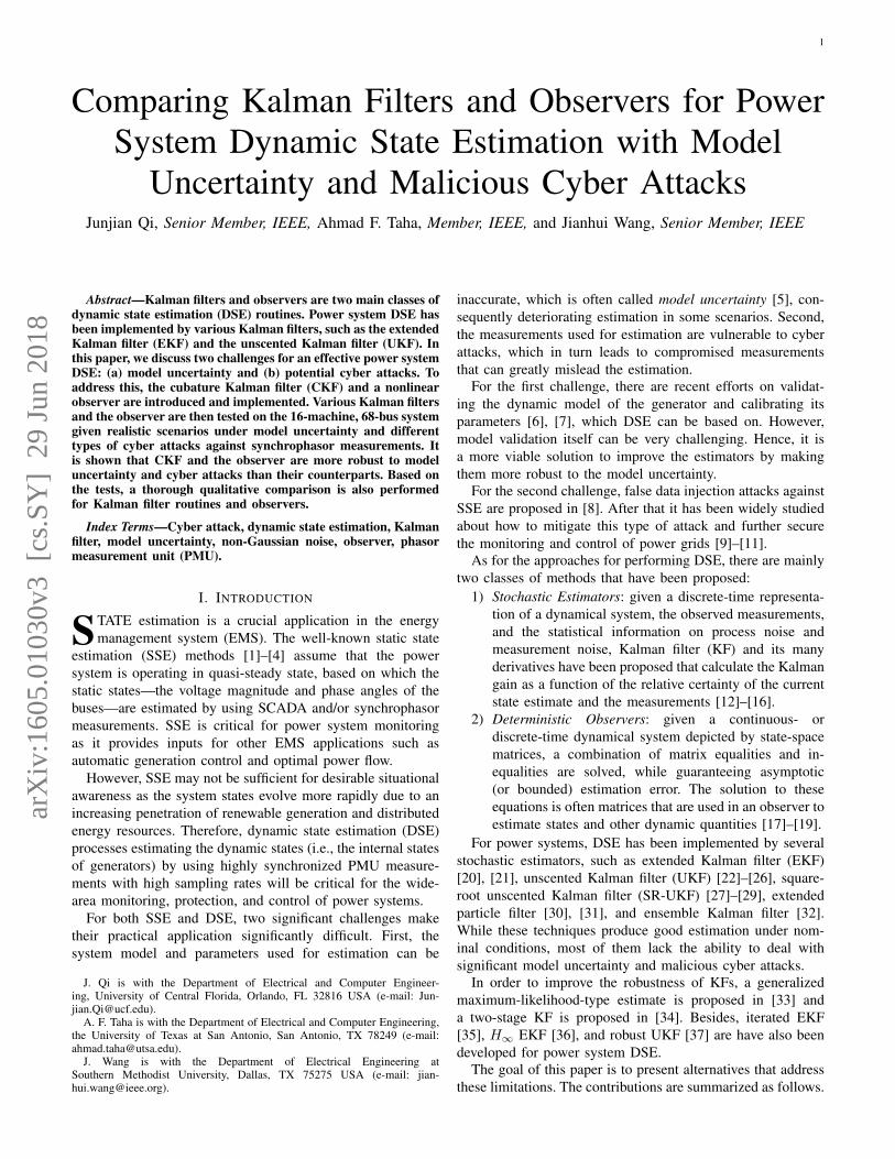
Data integrity attack is added to the first eight mea-surements, i.e., the real parts of the voltage phasors. Thecompromised measurements are obtained by scaling the realmeasurements by 0.6 and 1/0.6, respectively, for the firstfour and the last four measurements. The 2-norm of therelative error of the states, ||(x(t)−x(t))/x(t)||2, for differentestimation methods is shown in Fig. 1. It is seen that the errornorm for both CKF and the observer can quickly convergeamong which the observer converges faster, while the valuethat CKF converges to is slightly smaller in magnitude. Bycontrast, EKF, UKF, and SR-UKF do not perform as well.

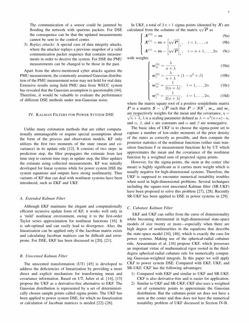
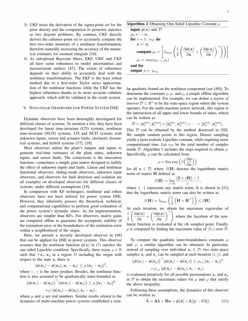
We also show the states estimation for Generator 1 in Fig.2. It is seen that the observer and CKF converge rapidly whilethe EKF fails to converge after 10 seconds. The estimation forUKF is separately shown in Fig. 3 because its estimated statesare far away from the real states. Note that the real systemdynamics are stable while the UKF estimation misled by thedata integrity attack indicates that the system is unstable.

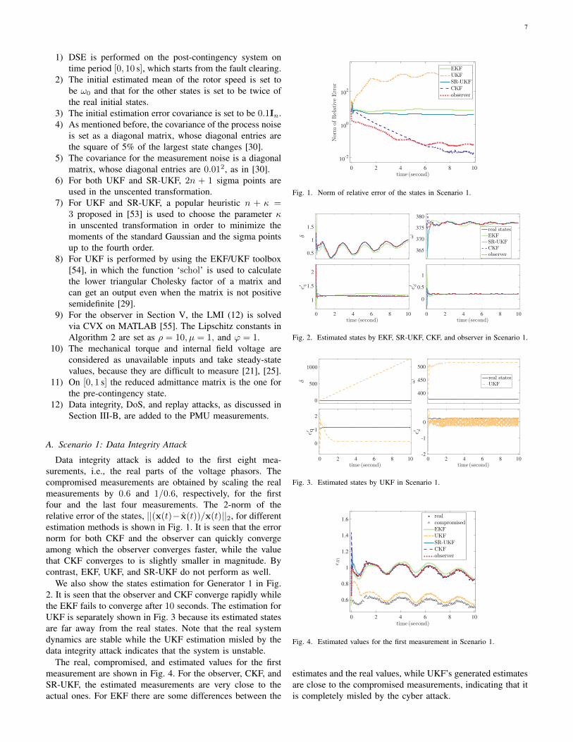
The real, compromised, and estimated values for the firstmeasurement are shown in Fig. 4. For the observer, CKF, andSR-UKF, the estimated measurements are very close to theactual ones. For EKF there are some differences between the

time (second)0 2 4 6 8 10

Norm

ofRelative

Error

10-2

100

102

EKFUKFSR-UKFCKFobserver

Fig. 1. Norm of relative error of the states in Scenario 1.


e′ q

1

1.5

2

δ

0.5

1

1.5


e′ d

0

0.5

1

ω

365

370

375

380

real statesEKFSR-UKFCKFobserver

Fig. 2. Estimated states by EKF, SR-UKF, CKF, and observer in Scenario 1.


e′ q

0

1

2

δ

0

500

1000


e′ d

-2

-1

0

ω

400

450

500

real statesUKF

Fig. 3. Estimated states by UKF in Scenario 1.


eR1

0.6

0.8

1

1.2

1.4

1.6realcompromisedEKFUKFSR-UKFCKFobserver

Fig. 4. Estimated values for the first measurement in Scenario 1.

estimates and the real values, while UKF’s generated estimatesare close to the compromised measurements, indicating that itis completely misled by the cyber attack.

8


Norm

ofRelativeError

10-2

100

102

104


(a)time (second)

0 2 4 6 8 10

Norm

ofRelativeError

10-2

100

102


(b)

Fig. 5. Norm of relative error of the states. (a) Scenario 2. (b) Scenario 3.

B. Scenario 2: DoS Attack and Scenario 3: Replay Attack

The first eight measurements are kept unchanged for t ∈[3 s, 6 s] to mimic the DoS attack in which case the updatedmeasurements cannot be sent to the control center due to, forexample, jammed communication between PMU to PDC orbetween PDC to the control center [42].

Replay attack is added on the first eight measurements forwhich there is yi(t) = yi(t− 3) for t ∈ [3 s, 6 s].

The 2-norm of the relative error of the states is shown inFig. 5 and the results are very similar to those in Scenario 1.

C. Discussion on Model Uncertainty Estimation

We take Scenario 1 as an example to discuss the perfor-mance of different methods in dealing with model uncertainty.The states of the system with and without model uncertainty,including unknown inputs, unavailable inputs, and parameterinaccuracy, are separately denoted by x and x0, which areshown in Fig. 6. The difference between x and x0, x − x0,is shown in Fig. 7. The estimated model uncertainty forGenerator 1 by EKF, SR-UKF, CKF, and the observer is shownin Fig. 8 and that for UKF is shown in Fig. 9. It is seenthat SR-UKF, CKF, and the observer can estimate the modeluncertainty pretty well while the EKF does not perform as welland the UKF has the worst performance for which the modeluncertainty estimation is largely misled by the data integrityattack.


e′ q

1.13

1.14

1.15

1.16

δ

0.2

0.4

0.6

0.8

1


e′ d

0.18

0.2

0.22

0.24

ω

376

377

378

379x0

x

Fig. 6. System states with and without model uncertainty in Scenario 1.


e′ q

×10-3

-1

0

1

δ

-0.1

-0.05

0

0.05

0.1


e′ d

-0.01

-0.005

0

0.005

0.01

ω

-0.4

-0.2

0

0.2

Fig. 7. The x− x0 in Scenario 1.


e′ q

0

0.5

1

δ

0

0.5

1


e′ d

-0.5

0

0.5

1

ω

-15

-10

-5

0

x− x0

EKFSR-UKFCKFobserver

Fig. 8. Estimated model uncertainty for EKF, SR-UKF, CKF, and the observerin Scenario 1.


e′ q

-2

-1

0

1

2

δ

-500

0

500

1000

1500


e′ d

-3

-2

-1

0

1

ω

-50

0

50

100

150

x− x0

UKF

Fig. 9. Estimated model uncertainty for UKF in Scenario 1.

D. Discussion on Cyber Attack Detection

The normalized innovation ratio of the jth measurement attime step k is defined as the ratio between the deviation of itsactual measurement from the predicted measurement and theexpected standard deviation [22], [24], [25]:

λk,j =yk,j − yk|k−1,j√

Pyy,k|k−1,j, (15)

where Pyy,k|k−1,j is the jth diagonal element of the measure-ment covariance.

The normalized innovation ratio for all of the measurementsfor EKF, UKF, SR-UKF, and CKF in Scenario 1 are shownin Fig. 10. It is seen that for EKF and UKF the normalizedinnovation ratios of a few uncompromised measurements

9


λ

-500

0

500

1000

1500

2000

2500

compromiseduncompromised

(a)


λ

-2000

-1000

0

1000

2000


(b)


λ

-500

0

500


(c)


λ

-100

0

100

200

300


(d)

Fig. 10. Cyber attack detection in Scenario 1 for (a) EKF, (b) UKF, (c)SR-UKF, and (d) CKF.

are greater than those for the compromised measurements,which means that EKF and UKF cannot correctly detect thecompromised measurements. For SR-UKF and CKF, aftera few seconds (in the first second some uncompromisedmeasurements can have bigger normalized innovation ratiosmainly because the parameters used for estimation in thattime period are inaccurate), the normalized innovation ratiosfor compromised measurements are significantly greater thanthose for the uncompromised ones, and the compromisedmeasurements can be detected by a properly chosen threshold.Compared to SR-UKF, CKF has a better performance. ForScenarios 2–3 the results are similar and are not presented.

For the observer, since there is no measurement covariancewe will detect cyber attacks against the measurements directlyusing the measurement innovation yk,j − yk|k−1,j , which isshown in Fig. 11a for Scenario 1. It is seen that after thefirst second in which the parameters are inaccurate the mea-surement innovation of the compromised measurements aresignificantly greater than those of the uncompromised ones andthus the compromised measurements can be easily detected.In Fig. 11b we also show the different between the real andestimated measurements, y0−y. For both the compromised anduncompromised measurements, the estimated measurementsfrom the observer can almost immediately converge to thereal measurements after the first second.

In Fig. 12 we show the measurement innovation of theobserver for Scenario 2 (Fig. 12a) and Scenario 3 (Fig. 12b),which indicates that the compromised measurements can alsobe detected by the observer.

E. Non-Gaussian Measurement Noise

We performed DSE under data integrity attack in Scenario 1with non-Gaussian measurement noise, including the Laplacenoise and Cauchy noise.


y−y

-1

-0.5

0

0.5

1

1.5


(a)


y0−y

-1

-0.5

0

0.5

1

1.5


(b)

Fig. 11. Norm of relateive error of the states. (a) attack detection and realand estimated measurements for the observer in Scenario 1.


y−

y-1

-0.5

0

0.5

1

1.5compromiseduncompromised

(a)


y−

y

-1

-0.5

0

0.5

1

1.5compromiseduncompromised

(b)

Fig. 12. Cyber attack detection in Scenario 2 and Scenario 3 for the observer.

Laplace noise with mean m and scale s is generated byrLaplace = m− s sgn(U1) ln(1− 2|U1|), (16)

where m is set to be zero, s is chosen as 0.02, and U1 is arandom number sampled from a uniform distribution in theinterval (−0.5, 0.5].

Cauchy noise is obtained by sampling the inverse cumula-tive distribution function of the distribution

rCauchy = a+ b tan(π(U2 − 0.5)

), (17)

where a = 0 and b = 10−4 are the location and scaleparameters, and U2 is randomly sampled from the uniformdistribution on the interval (0, 1).

The norms of the relative error of the states under Laplaceand Cauchy noises are shown in Fig. 13. Similar to the casewith Gaussian noise, the observer and CKF also outperformthe other methods. Under Laplace noise, the performance ofdifferent methods are similar to that under Gaussian noise.However, under Cauchy noise that has a super-heavy taileddistribution with no defined moments, the performance of allmethods degrade, converging to a much bigger norm of relativeerror of the states.

F. Computational Efficiency

For the above three scenarios, the time for estimation bydifferent methods is listed in Table I. It is seen that EKF andthe observer are more efficient than the other methods whileCKF is the least efficient. Note that the time reported here isfrom MATLAB implementations. It can be greatly reduced bymore efficient, such as C-based implementations.

10

0 2 4 6 8 1010-2

100

102

104

(a)

0 2 4 6 8 10

100

105

(b)

Fig. 13. Norm of relative error of the states under different measurementnoises. (a) Laplace noise and (b) Cauchy noise.

TABLE ITIME FOR PERFORMING ESTIMATION FOR 10 SECONDS

EKF UKF SR-UKF CKF observer

4.0 s 11.2 s 11.6 s 9.9 s 5.8 s

VII. COMPARING KALMAN FILTERS AND OBSERVERS

Here, various functionalities of DSE methods and theirstrengths and weaknesses relative to each functionality arepresented based on (a) the technical, theoretical capabilitiesand (b) experimental results in Section VI.

• Nonlinearities in Dynamics: UKF, SR-UKF, CKF, andthe observer in Section V all work on nonlinear systemswhile EKF assumes linearized system dynamics. Besides,the presented observer uses linearized measurement func-tions for design but directly uses nonlinear measurementfunctions for estimation.

• Solution Feasibility: The main principle that governs thedesign of most observers is based on finding a matrixgain satisfying a certain condition, such as a solution toa matrix inequality. The state estimates are guaranteedto converge to the actual ones if a solution to the LMIexists. In contrast, KF methods do not require that.

• Unknown Initial Conditions: Most observer designs areindependent on the knowledge of the initial conditions ofthe system. However, if the estimator’s initial conditionis chosen to be reasonably different from the actual one,estimates from KF might not converge to the actual ones.

• Robustness to Model Uncertainty and Cyber Attacks: Theobserver in Section V and the CKF outperforms UKF(SR-UKF) and EKF in the state estimation under modeluncertainty and attack vectors. The observer is robustto model uncertainties because it only assumes that thenonlinearities in the power system dynamics (i.e., φ(x))satisfy the quadratic inner-boundedness and the one-sidedLipschitz condition. As in Section IV-C, CKF is morerobust mostly due to its more accurate cubature approach,which, however, requires more careful investigation.

• Tolerance to Process and Measurement Noise: The ob-server in Section V is tolerant to measurement and pro-cess noise similar to those assumed for KFs. By design,the KF techniques are developed to deal with such noise.

• Convergence Guarantees: Observers have theoreticalguarantees for convergence while for the KF techniquesthere is no strict proof to guarantee that the estimationconverges to actual states.

• Numerical Stability: Observers do not have numericalstability problems while UKF can encounter numericalinstability because the estimation error covariance matrixis not always guaranteed to be positive semi-definite [29].

• Tolerance to Parametric Inaccuracy: KF-based methodscan tolerate inaccurate parameters to some extent. Dy-namic observers deal with parametric uncertainty in thesense that all uncertainties can be augmented to theunknown input component in the state dynamics (Bww).

• Computational Complexity: The CKF, UKF (SR-UKF),and EKF all have computational complexity of O(n3)[16], [27]. Since the observers’ matrix gains are obtainedoffline by solving LMIs, observers are easier to imple-ment as only the dynamics are needed in the estimation.

VIII. CONCLUSION AND FUTURE WORK

In this paper, we discuss different DSE methods by pre-senting an overview of state-of-the-art estimation techniquesand developing alternatives, including the CKF and dynamicobservers, to address major limitations of existing methodssuch as intolerance to inaccurate system model and maliciouscyber attacks. The proposed methods are extensively testedon a 16-machine 68-bus power system, under significantmodel uncertainty and cyber attacks against the synchrophaosrmeasurements. It is shown that the CKF and the observer aremore robust to model uncertainty and cyber attacks.

Based on the theoretical capabilities and the experimentalresults, we summarize the strengths and weaknesses of differ-ent estimation techniques especially for power system DSE.We acknowledge that some of these comparisons, such astolerance to process and measurement noise, are mostly basedon numerical results. As future work we will more theoreti-cally investigate and analyze the observer in comparison withKalman filters.

REFERENCES

[1] A. Monticelli, “Electric power system state estimation,” Proc. IEEE,vol. 88, no. 2, pp. 262–282, Feb. 2000.

[2] A. Abur and A. Exposito, Power System State Estimation: Theory andImplementation, ser. Power Engineering (Willis). CRC Press, 2004.

[3] G. He, S. Dong, J. Qi, and Y. Wang, “Robust state estimator based onmaximum normal measurement rate,” IEEE Trans. Power Syst., vol. 26,no. 4, pp. 2058–2065, Nov. 2011.

[4] J. Qi, G. He, S. Mei, and F. Liu, “Power system set membership stateestimation,” in IEEE Power and Energy Society General Meeting, Jul.2012, pp. 1–7.

[5] K. Zhou, J. C. Doyle, and K. Glover, Robust and Optimal Control.Prentice hall New Jersey, 1996.

[6] Z. Huang, P. Du, D. Kosterev, and S. Yang, “Generator dynamic modelvalidation and parameter calibration using phasor measurements at thepoint of connection,” IEEE Trans. Power Syst., vol. 28, no. 2, pp. 1939–1949, May 2013.

[7] M. Ariff, B. Pal, and A. Singh, “Estimating dynamic model parametersfor adaptive protection and control in power system,” IEEE Trans. PowerSyst., vol. 30, no. 2, pp. 829–839, Mar. 2015.

11

[8] Y. Liu, P. Ning, and M. K. Reiter, “False data injection attacks againststate estimation in electric power grids,” ACM Trans. Inf. Syst. Secur.,vol. 14, no. 1, pp. 13:1–13:33, Jun. 2011.

[9] R. J. T. O. Kosut, L. Jia and L. Tong, “Malicious data attacks on thesmart grid,” IEEE Trans. Smart Grid, vol. 2, no. 4, pp. 645–658, Dec.2011.

[10] G. D. O. Vukovic, K. C. Sou and H. Sandberg, “Network-awaremitigation of data integrity attacks on power system state estimation,”IEEE J. Sel. Area Comm., vol. 30, no. 6, pp. 1108–1118, Jul. 2012.

[11] W. Y. D. A. N. Z. W. Z. Q. Yang, J. Yang, “On false data-injection attacksagainst power system state estimation: modeling and countermeasures,”IEEE Tran. Parallel Distrib. Syst., vol. 25, no. 3, pp. 717–729, Mar.2014.

[12] R. E. Kalman, “A new approach to linear filtering and predictionproblems,” J. Fluids Eng., vol. 82, no. 1, pp. 35–45, Mar. 1960.

[13] A. H. Jazwinski, Stochastic Processes and Filtering Theory. CourierCorporation, 2007.

[14] S. J. Julier and J. K. Uhlmann, “New extension of the Kalman filter tononlinear systems,” in AeroSense’97. International Society for Opticsand Photonics, Jul. 1997, pp. 182–193.

[15] S. Julier and J. Uhlmann, “Unscented filtering and nonlinear estimation,”Proc. IEEE, vol. 92, no. 3, pp. 401–422, Mar. 2004.

[16] I. Arasaratnam and S. Haykin, “Cubature Kalman filters,” IEEE Trans.Autom. Control, vol. 54, no. 6, pp. 1254–1269, Jun. 2009.

[17] W. Kang, A. J. Krener, M. Xiao, and L. Xu, “A survey of observers fornonlinear dynamical systems,” in Data Assimilation for Atmospheric,Oceanic and Hydrologic Applications (Vol. II). Springer, 2013, pp.1–25.

[18] A. Radke and Z. Gao, “A survey of state and disturbance observers forpractitioners,” in American Control Conference, Jun. 2006, pp. 5183–5188.

[19] Z. Hidayat, R. Babuska, B. D. Schutter, and A. Nez, “Observers forlinear distributed-parameter systems: A survey,” in IEEE InternationalSymposium on Robotic and Sensors Environments (ROSE), Sept. 2011,pp. 166–171.

[20] Z. Huang, K. Schneider, and J. Nieplocha, “Feasibility studies of apply-ing Kalman filter techniques to power system dynamic state estimation,”in Proc. 2007 Power Engineering Conf., Dec. 2007, pp. 376–382.

[21] E. Ghahremani and I. Kamwa, “Dynamic state estimation in powersystem by applying the extended Kalman filter with unknown inputsto phasor measurements,” IEEE Trans. Power Syst., vol. 26, no. 4, pp.2556–2566, Nov. 2011.

[22] G. Valverde and V. Terzija, “Unscented Kalman filter for power systemdynamic state estimation,” IET Gener. Transm. Distrib., vol. 5, no. 1,pp. 29–37, Jan. 2011.

[23] E. Ghahremani and I. Kamwa, “Online state estimation of a synchronousgenerator using unscented Kalman filter from phasor measurementsunits,” IEEE Trans. Energy Convers., vol. 26, no. 4, pp. 1099–1108,Dec. 2011.

[24] S. Wang, W. Gao, and A. Meliopoulos, “An alternative method for powersystem dynamic state estimation based on unscented transform,” IEEETrans. Power Syst., vol. 27, no. 2, pp. 942–950, May 2012.

[25] A. Singh and B. Pal, “Decentralized dynamic state estimation in powersystems using unscented transformation,” IEEE Trans. Power Syst.,vol. 29, no. 2, pp. 794–804, Mar. 2014.

[26] K. Sun, J. Qi, and W. Kang, “Power system observability and dynamicstate estimation for stability monitoring using synchrophasor measure-ments,” Control Engineering Practice, vol. 53, pp. 160–172, Aug. 2016.

[27] R. Van Der Merwe and E. A. Wan, “The square-root unscented Kalmanfilter for state and parameter-estimation,” in Proc. Int. Conf. Acoustics,Speech, and Signal Processing, vol. 6, May 2001, pp. 3461–3464.

[28] J. Qi, K. Sun, and W. Kang, “Optimal PMU placement for power systemdynamic state estimation by using empirical observability gramian,”IEEE Trans. Power Syst., vol. 30, no. 4, pp. 2041–2054, Jul. 2015.

[29] J. Qi, K. Sun, J. Wang, and H. Liu, “Dynamic state estimation formulti-machine power system by unscented Kalman filter with enhancednumerical stability,” IEEE Trans. Smart Grid, vol. 9, no. 2, pp. 1184–1196, Mar. 2018.

[30] N. Zhou, D. Meng, and S. Lu, “Estimation of the dynamic states ofsynchronous machines using an extended particle filter,” IEEE Trans.Power Syst., vol. 28, no. 4, pp. 4152–4161, Nov. 2013.

[31] Y. Cui and R. Kavasseri, “A particle filter for dynamic state estimationin multi-machine systems with detailed models,” IEEE Trans. PowerSyst., vol. 30, no. 6, pp. 3377–3385, Nov. 2015.

[32] N. Zhou, D. Meng, Z. Huang, and G. Welch, “Dynamic state estimationof a synchronous machine using pmu data: A comparative study,” IEEETrans. Smart Grid, vol. 6, no. 1, pp. 450–460, Jan. 2015.

[33] M. A. Gandhi and L. Mili, “Robust kalman filter based on a general-ized maximum-likelihood-type estimator,” IEEE Trans. Signal Process.,vol. 58, no. 5, pp. 2509–2520, May 2010.

[34] G. B. J. Zhang, G. Welch and Z. Huang, “A two-stage kalman filterapproach for robust and real-time power system state estimation,” IEEETrans. Sustain. Energy, vol. 5, no. 2, pp. 629–636, Apr. 2014.

[35] J. Zhao, M. Netto, and L. Mili, “A robust iterated extended kalman filterfor power system dynamic state estimation,” IEEE Trans. Power Syst.,vol. 32, no. 4, pp. 3205–3216, July 2017.

[36] J. Zhao, “Dynamic state estimation with model uncertainties using H∞extended Kalman filter,” IEEE Trans. Power Syst., vol. 33, no. 1, pp.1099–1100, Jan 2018.

[37] J. Zhao and L. Mili, “Robust unscented kalman filter for power systemdynamic state estimation with unknown noise statistics,” IEEE Trans.Smart Grid, pp. 1–1, 2017.

[38] J. W. A. F. Taha, J. Qi and J. H. Panchal, “Risk mitigation for dynamicstate estimation against cyber attacks and unknown inputs,” IEEE Trans.Smart Grid, vol. 9, no. 2, pp. 886–899, Mar. 2018.

[39] A. Hajnoroozi, F. Aminifar, H. Ayoubzadeh et al., “Generating unitmodel validation and calibration through synchrophasor measurements,”IEEE Trans. Smart Grid, vol. 6, no. 1, pp. 441–449, Jan. 2015.

[40] J. Chen and R. Patton, Robust Model-Based Fault Diagnosis for DynamicSystems. Springer Publishing Company, Incorporated, 2012.

[41] A. Pertew, H. Marquezz, and Q. Zhao, “Design of unknown inputobservers for lipschitz nonlinear systems,” in Proc. American ControlConf., Jun. 2005, pp. 4198–4203.

[42] “Electric Sector Failure Scenarios and Impact Analyses,” Electric PowerResearch Institute (EPRI), Tech. Rep., Jun. 2014.

[43] S. Sridhar, A. Hahn, and M. Govindarasu, “Cyber–physical systemsecurity for the electric power grid,” Proc. IEEE, vol. 100, no. 1, pp.210–224, Jan. 2012.

[44] S. Wang, J. Zhao, Z. Huang, and R. Diao, “Assessing Gaussian assump-tion of pmu measurement error using field data,” IEEE Trans. PowerDel., vol. PP, no. 99, pp. 1–1, 2017.

[45] J. K. Uhlmann, “Simultaneous map building and localization for realtime applications,” transfer thesis, Univ. Oxford, Oxford, UK, 1994.

[46] R. Bellman and R. Bellman, Adaptive Control Processes: A GuidedTour, ser. ’Rand Corporation. Research studies. Princeton UniversityPress, 1961.

[47] I. A. S. A. Gadsden, M. Al-Shabi and S. R. Habibi, “Combined cubaturekalman and smooth variable structure filtering: A robust nonlinearestimation strategy,” Signal Processing, vol. 96, pp. 290–299, Mar. 2014.

[48] W. Zhang, H. Su, H. Wang, and Z. Han, “Full-order and reduced-order observers for one-sided lipschitz nonlinear systems using riccatiequations,” Commun. Nonlinear Sci. Numer. Simul., vol. 17, no. 12, pp.4968–4977, Dec. 2012.

[49] D. Siljak, D. Stipanovic, and A. Zecevic, “Robust decentralized tur-bine/governor control using linear matrix inequalities,” IEEE Trans.Power Syst., vol. 17, no. 3, pp. 715–722, Aug. 2002.

[50] J. Qi, J. Wang, H. Liu, and A. D. Dimitrovski, “Nonlinear modelreduction in power systems by balancing of empirical controllabilityand observability covariances,” IEEE Trans. Power Syst., vol. 32, no. 1,pp. 114–126, Jan. 2017.

[51] M. Vidyasagar, Nonlinear Systems Analysis. SIAM, 2002.[52] J. H. Chow and K. W. Cheung, “A toolbox for power system dynamics

and control engineering education and research,” IEEE Trans. PowerSyst., vol. 7, no. 4, pp. 1559–1564, Nov. 1992.

[53] S. Julier, J. Uhlmann, and H. F. Durrant-Whyte, “A new method forthe nonlinear transformation of means and covariances in filters andestimators,” IEEE Trans. Autom. Control, vol. 45, no. 3, pp. 477–482,Mar. 2000.

[54] J. Hartikainen, A. Solin, and S. Sarkka, “Optimal filtering with kalmanfilters and smoothers,” Department of Biomedica Engineering and Com-putational Sciences, Aalto University School of Science, 16th August,Aug. 2011.

[55] M. Grant and S. Boyd, “CVX: Matlab software for disciplined convexprogramming,” Tech. Rep., Sept. 2013.

comparing kalman filters and observers for power system

Documents