Munich Personal RePEc Archive

Comparing Monopoly and Duopoly on a

Two-Sided Market without Product

Differentiation

Böhme, Enrico and Müller, Christopher

Goethe Universität Frankfurt

29 June 2010

Online at https://mpra.ub.uni-muenchen.de/23568/

MPRA Paper No. 23568, posted 30 Jun 2010 01:40 UTC

* Both authors are from the Chair of Public Finance, Department of Economics, Frankfurt University,

Grüneburgplatz 1, D-60323 Frankfurt am Main, Germany. E-mails: boehme@econ.uni-frankfurt.de,

christmu@wiwi.uni-frankfurt.de. Authors’ names in alphabetical order. Corresponding author: Enrico Böhme.

Comparing Monopoly and Duopoly on a Two-Sided Market

without Product Differentiation

Enrico Böhme, Christopher Müller*

Johann Wolfgang Goethe-University, Frankfurt

Manuscript version: June 29, 2010

Abstract

We propose both a monopoly and a duopoly model of a two-sided market. Both settings are

fully comparable, as we impose a homogeneous good produced at zero costs without capacity

constraints, as well as identical parameterization of market sizes. We determine the duopoly

equilibrium and the monopoly optimum in terms of the parameters and obtain solutions with

and without subsidization (prices below marginal cost) of one market side. We show that

there exists a continuum of economically plausible parameter sets for which duopoly

equilibrium prices exceed optimal monopoly prices and one with no observable price effect of

competition, i.e. one where optimum and equilibrium prices become equal. Despite the fact

that virtually everything except for the number of platform operators is identical in the latter

situations, total demand on both market sides in the duopoly market exceeds total demand in

the monopoly market. Furthermore, even though there is no observable price effect, there is

still a competitive effect in so far that total profits in the duopoly equilibrium are strictly

smaller than monopoly profits. The relationship of total welfare is ambiguous in subsidization

cases, while it is strictly greater in duopoly, if no subsidization takes place. Our results

sharply contradict economic intuition and common economic knowledge from one-sided

markets.

Keywords: two-sided markets, platform competition, price-concentration relationship,

welfare analysis

JEL Classification: D42, D43, K20, L12, L13, L51

2

1. Introduction and Literature Review

The well-known literature on network effects studies markets, in which firms face a group of

more or less homogeneous customers with externalities emerging “within” this group. On the

other hand, there are many markets, in which firms face two or more distinct and

distinguishable customer groups with externalities emerging “in between” these groups. In

media economics this setting describes the relation of the media provider, media consumers,

and advertisers. There it is termed “circulation industry” (Chaudhri (1998)) or “dual product

market” (Picard (1989)). In Industrial Organization, this setting became prominent as “two-

sided market” following the seminal analyses by Rochet and Tirole (2003) and Caillaud and

Jullien (2003).

Rochet and Tirole (2003) instance credit cards as an example of a two-sided market:

Consumers and retailers constitute two distinct and distinguishable groups of customers to a

credit card provider. The number of retailers who wish to be connected to a specific credit

card network is affected by the number of consumers who wish to pay using this credit card.

Vice versa, the number of consumers who apply for a specific credit card is affected by the

number of retailers who accept it. The externality is positive for both market sides in this

example: Increasing demand by one group increases demand by the other group.

The features of two-sided markets are, however, hard to generalize. For instance, two-sided

markets might as well be characterized by negative externalities or externalities might be

positive for one side and negative for the other side, as will be discussed for the example of

advertising further below.

Furthermore, credit cards are a club good to both market sides, which means that specific

consumers and retailers can be excluded from the service, but there is no rivalry in

consumption of a credit card service. Obviously, other goods feature different characteristics,

that is, they might be either rival or non-rival in consumption, and they might be excludable

or non-excludable or their characteristics might depend on the market side. For instance free-

to-air radio broadcasts are a public good (non-rival, non-excludable) to the audience, but since

advertising slots are naturally limited by the available air time, advertising slots are a private

good (rival, excludable) to advertisers.

Third, credit cards are goods that allow for joint consumption also known as “multi-homing”.

That is, a consumer might well own more than one credit card at the same time (and even use

more than one card for the same transaction by splitting the amount invoiced), and retailers

might accept more than one card. Other two-sided markets require one or both market sides to

decide for exactly one provider (or, of course, none at all). For instance, a moviegoer has to

3

decide for exactly one cinema on a Saturday night, but a firm can place advertisements in

more than one movie theater.

Fourth, credit cards are a homogeneous product. That is, differences in utility from using the

one or the other credit card service only stem from price differences and the two-sided market

effect, i.e. the diffusion of a specific service on the other market side. Other two-sided

markets allow for product differentiation, e.g. in the newspaper market, there might be

differentiation according to political views or intellectual level of the target group.

Finally, there are differences in strategic interaction in terms of timing (simultaneous or

sequential action) and the strategic variables (price or quantity) used by the players in a two-

sided market game.

Because of this, the literature on two-sided markets tailors models around specific examples.

Armstrong's (2006) study provides a variety of constellations, including those studied by

Caillaud and Jullien (2003) and Rochet and Tirole (2003). Armstrong (2006) derives optimal

pricing rules for monopoly and duopoly markets in terms of elasticities and provides some

applications, e.g. to advertising. He finds that there is no difference in advertising prices

between monopolies and oligopolies, given media consumers must single-home and

advertisers can multi-home - a constellation he calls “competetive bottlenecks”. He argues

that competition only emerges on the market for media consumers: Media providers compete

for consumers, since advertisers’ demand depends on the number of consumers that are

exposed to the advertisement, and consumers need to single-home. However, media providers

are still monopolists when providing their consumers’ attention to the advertiser, because a

specific consumer can ony be reached by advertising with the provider this consumer chose.

Nilssen and Sørgard (2001) and Gabszewicz et al. (1999) study TV advertising as a sequential

two-sided market game in which advertising revenues finance programming investments of

TV stations. Nilssen and Sørgard (2001) show -in contrast to Armstrong's (2006) result- that

in this case the advertising price in a symmetric duopoly is always lower than in a monopoly.

Although the price is lower in duopoly, the total amount of advertising might be lower than in

monopoly. This is because each duopolist’s programming investment is lower than the

monopolist’s one. Lower programming investment implies lower program quality which in

turn implies a lower number of viewers. This lower number of viewers might offset the

increasing demand for advertising caused by the lower duopoly advertising price, and cause a

decrease in the total amount of advertising.

4

While there seems to be broad consensus in that the externality of a large audience on

advertising demand is positive, there is some dissent about the effect in the other direction.

Theoretical models, e.g. those of Nilssen and Sørgard (2001) and Gabszewicz et al. (1999)

mentioned above, usually assume that media consumers wish to consume the media content

only, and are “coerced” to consume advertising as well. Empirical results support this “ad-

aversion” assumption for television viewers (see e.g. Danaher (1995), Wilbur (2007)), but

reject it for print media, where readers’ attitude towards advertising seems to be driven by the

informative value of the advertisement (Kaiser and Song (2009), Rysman (2004)). This

example supports our earlier statement that it is hard to generalize two-sided market models,

and the approach of the literature to tailor models to specific examples.

Chaudhri (1998) and Dewenter (2006) develop two-sided market models of a newspaper

monopoly. Comparing the optimal monopoly advertising and consumer prices and the

competitive market outcome, Chaudhri (1998) finds that the optimal monopoly consumer

price might be even lower than the competitive one, because increased circulation on the

monopoly market yields higher advertising revenue. However, Chaudhri (1998) does not

model demand explicitly and ignores the feedback effect of circulation on advertising

demand. The increase in advertising revenue in his analysis stems from the pricing model

(per-contact-pricing) for advertising. Advertising demand itself is not affected by circulation.

Häckner and Nyberg (2008), and similarly Anderson and Gabszewicz (2006), also having

newspaper markets in mind, propose a two-sided market model with endogeneous market

structure (duopoly or monopoly). In a simultaneous game, they examine conditions for

symmetric and asymmetric duopoly equilibria as well as conditions for a natural monopoly.

Product differentiation is a crucial feature of their model that drives the resulting market

structure. Another basic assumption through most of their study is a positive externality of

advertising on consumer demand, i.e. they assume that readers like advertising. In case of a

negative effect of advertising on consumers, however, they find that only symmetric

equilibria can exist.

The aim of the present paper is to compare prices on two-sided monopoly and duopoly

markets in more detail than it was done in previous literature. Unlike previous literature, we

neither allow for product differentiation, since it would make us compare apples and oranges,

nor do we impose structural differences in terms of costs or capacity constraints that might

favor the one or the other market structure. We also sacrifice generality by restricting our

5

model to a “competitive bottleneck” scenario and by introducing explicit utility functions for

the agents on both market sides, which enables us to parameterize our model and to obtain

results in terms of the parameters. We use these results to study the behavior of the outcomes

in monopoly and duopoly depending on the parameters. We are especially interested in the

question of whether there are economically plausible parameter sets that equalize prices in

monopoly and duopoly or yield even higher prices in duopoly than in monopoly, which would

sharply contradict economic intuition and common economic knowledge from one-sided

markets.

The question of price changes with regard to market structure becomes relevant when policy

makers consider subsidies in order to attract new entrants to given monopoly markets.

Reversely, antitrust authorities need to assess the impact of mergers on prices. A positive

correlation of price and market concentration is also the fundamental assumption of the

empirical price-concentration literature that aims at measuring the price effect of market

concentration.

The paper generally contributes to the literature on two-sided markets by explicitly comparing

monopoly and duopoly outcomes on a competitive bottleneck two-sided private good market.

It is therefore complementary to Nilssen and Sørgard (2001) who study a two-sided market

where the good is public to one side, but private to the other side of the market, Weyl (2006),

who studies pricing in the Rochet and Tirole (2003) framework, and a refinement of

Armstrong's (2006) “competitive bottleneck” scenario.

To help the reader grasp the economic intuition behind the model, we will follow the common

habit of the literature and refer from time to time to a specific example, namely to the one of

mainstream movie theaters. In contrast to the aforementioned TV broadcasts, movie theaters

provide a private good to both advertisers and moviegoers, since individuals on both market

sides can easily be excluded. A consumer feels rivalry in consumption at least if her favorite

seat is already taken. Advertisers feel rivalry, because consumer attention will decrease the

more advertisements are shown. The example fits the competitive bottleneck scenario,

because by nature consumers can only visit one cinema at the same time, hence they must

single-home, while advertisers can place advertisements in more than one cinema, hence they

can multi-home. Mainstream movie theaters are usually large multiplex facilities that feature

the latest projection and audio technology and the same portfolio of the latest movies.

6

Therefore, in the duopoly case, an average consumer will have no intrinsic preference for the

one or the other cinema: both facilities are homogeneous.

The paper is constructed as follows: First we develop a monopoly model and derive the

monopolist’s optimal pricing policy. Second, we suggest a model of duopolistic competition

that is founded on the same assumptions as the monopoly model, thus being fully comparable

to the monopoly case. In Section 4, we compare the equilibrium outcome in the duopoly case

and the monopolist’s optimum, and highlight some implications of our findings in Section 5.

2. The Monopoly Model

Consider a two-sided market for a consumption good that is offered in combination with

advertising. To foster intuition and readability, we will label customers on the one market side

“consumers” and customers on the other market side “advertisers”. In this section, we assume

that the market is served by a monopolistic platform operator. Similar to Anderson and

Gabszewicz (2006), we assume that consumers are homogeneous, except for their preference

for the good (e.g. “movie theater experience”). Let the individual net utility function be

additive-separable and given by

(1) { }1,0,)( ∈⋅−⋅⋅−⋅= ccccaccc qqpqdeqqU θ ,

where pc is the price for one unit of the consumption good, while θ is the taste parameter or

marginal willingness to pay, qc is the quantity, and e is a parameter for the influence of

advertising on the individual’s utility. Heterogeneous preferences for the good are reflected

by θ, which is assumed to be continuously distributed on the interval [0, msc], where msc > 0

determines the market size for the considered goods market. We limit qc to the values 0 and 1,

so that the individual’s decision problem is reduced to whether or not to consume a single unit

of the good (e.g. whether to go to the movies or not). Obviously, an individual demands the

good, if its net utility of doing so is greater than the net utility of refraining from

consumption, that is if

cacc pdeUU +⋅≥⇔=≥ θ0)0()1(

holds. Therefore, we obtain

(2) ( ) cac

ms

pde

acc pdemsddpdc

ca

−⋅−=⋅= ∫+⋅

θ1,

as the aggregated consumer demand function on the market.

7

Similar to Armstrong (2006), firms are assumed to generate constant net profits from

advertising. For simplicity, we assume advertisements to be standardized, so that firms only

decide whether or not to place an advertisement. Therefore a single firm’s advertising demand

qa is either 0 or 1. The firm’s net profit is given by

(3) { }1,0,)( ∈⋅⋅−⋅=Π aacaaaa qqdpqq µ ,

where pa is the per-contact advertising price, so that the firm has to pay pa·dc to place an

advertisement. µ is the parameter that describes the gross benefit of advertising. Firms are

assumed to be heterogeneous with respect to µ, and µ is assumed to be continuously

distributed on [0, msa·dc]. The expression msa·dc, with msa > 0 determines the size of the

advertising market. Note that the net profit to be gained from advertising and therefore the

size of the advertising market, depends on consumer demand. The economic intuition is

straightforward: The higher the demand for the good, the more consumers will be exposed to

the advertisement, the more profitable advertising becomes to a firm. Firms are willing to

advertise, if their net profit from doing so is positive, that is if

caaa dp ⋅≥⇔=Π≥Π µ0)0()1( .

Hence, total advertising demand is given by

(4) ( ) caca

dms

dp

caa dpdmsddpdca

aa

⋅−⋅=⋅= ∫⋅

⋅

µ1, .

This specific functional form assures that da(pa,0) = 0, which implies that there is no demand

for advertising if consumer demand is equal to zero.

Solving equations (2) and (4) for pc and pa, respectively, yields the inverse demand functions.

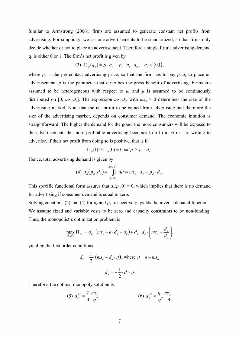
We assume fixed and variable costs to be zero and capacity constraints to be non-binding.

Thus, the monopolist’s optimization problem is

( )

−⋅⋅+−⋅−⋅=Π

c

aacacaccM

dd d

dmsddddemsd

ac ,max ,

yielding the first order conditions

( )η⋅−⋅= acc dmsd2

1, where amse −=η

η⋅⋅−= ca dd2

1

Therefore, the optimal monopoly solution is

(5) 24

2

η−⋅

= cM

c

msd (6)

42 −⋅

=ηη cM

a

msd

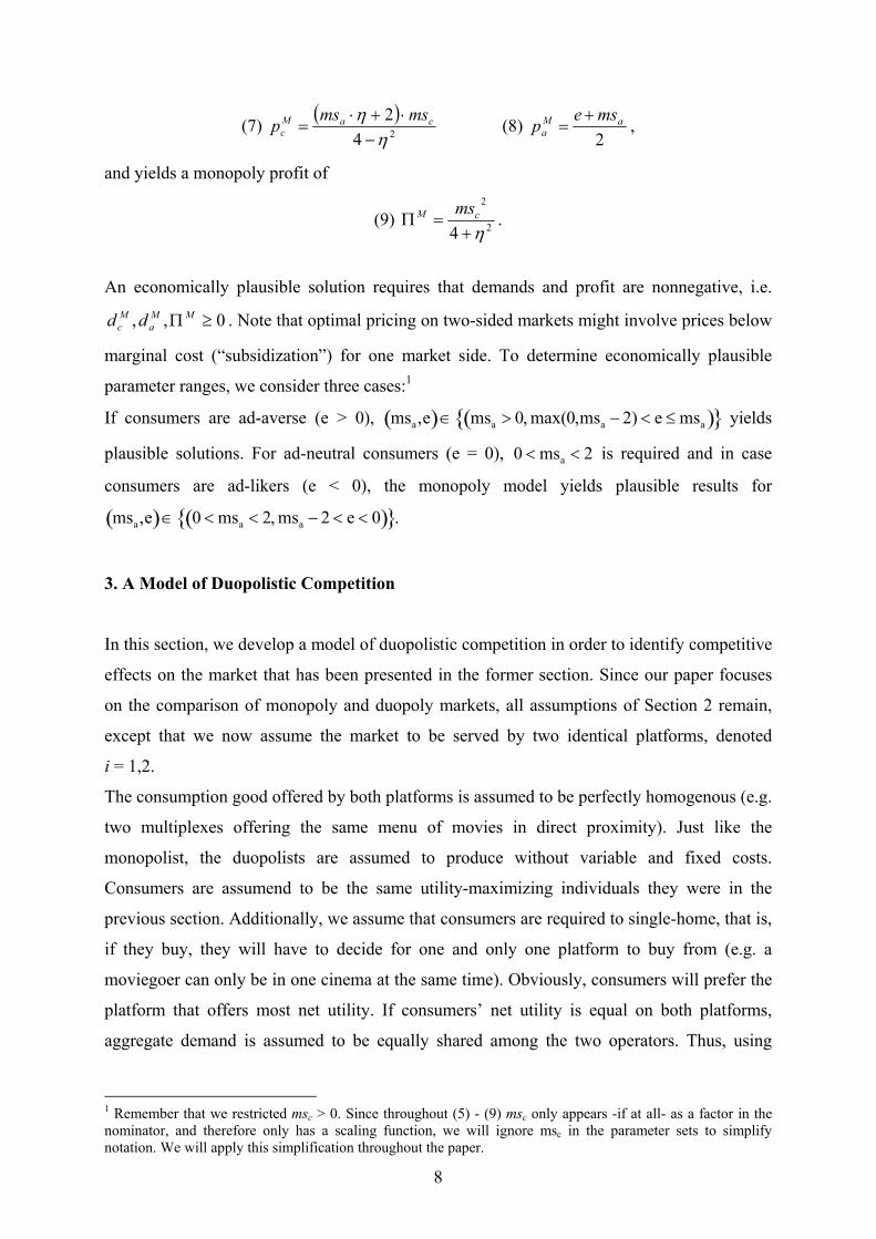
8

(7) ( )

24

2

ηη−

⋅+⋅= caM

c

msmsp (8)

2

aM

a

msep

+= ,

and yields a monopoly profit of

(9) 2

2

4 η+=Π cM ms

.

An economically plausible solution requires that demands and profit are nonnegative, i.e.

0,, ≥ΠMM

a

M

c dd . Note that optimal pricing on two-sided markets might involve prices below

marginal cost (“subsidization”) for one market side. To determine economically plausible

parameter ranges, we consider three cases:1

If consumers are ad-averse (e > 0), msa,e( )∈ msa > 0, max(0,msa − 2) < e ≤msa( ){ } yields

plausible solutions. For ad-neutral consumers (e = 0), 0 < msa < 2 is required and in case

consumers are ad-likers (e < 0), the monopoly model yields plausible results for

msa,e( )∈ 0 <msa < 2, msa − 2 < e < 0( ){ }.

3. A Model of Duopolistic Competition

In this section, we develop a model of duopolistic competition in order to identify competitive

effects on the market that has been presented in the former section. Since our paper focuses

on the comparison of monopoly and duopoly markets, all assumptions of Section 2 remain,

except that we now assume the market to be served by two identical platforms, denoted

i = 1,2.

The consumption good offered by both platforms is assumed to be perfectly homogenous (e.g.

two multiplexes offering the same menu of movies in direct proximity). Just like the

monopolist, the duopolists are assumed to produce without variable and fixed costs.

Consumers are assumend to be the same utility-maximizing individuals they were in the

previous section. Additionally, we assume that consumers are required to single-home, that is,

if they buy, they will have to decide for one and only one platform to buy from (e.g. a

moviegoer can only be in one cinema at the same time). Obviously, consumers will prefer the

platform that offers most net utility. If consumers’ net utility is equal on both platforms,

aggregate demand is assumed to be equally shared among the two operators. Thus, using

1 Remember that we restricted msc > 0. Since throughout (5) - (9) msc only appears -if at all- as a factor in the

nominator, and therefore only has a scaling function, we will ignore msc in the parameter sets to simplify

notation. We will apply this simplification throughout the paper.

9

equation (1) for qc = 1 and equation (2), the consumer demand function platform operator i

faces is

(10) ( ) jiji

pdepdeforpdems

pdepdeforpdems

pdepdefor

dpd

j

c

j

a

i

c

i

a

i

c

i

ac

j

c

j

a

i

c

i

a

i

c

i

ac

j

c

j

a

i

c

i

a

i

a

i

c

i

c ≠=

−⋅−>−⋅−−⋅−

−⋅−=−⋅−−⋅−

−⋅−<−⋅−

= ,2,1,2

0

,

θθ

θθ

θθ

Unlike consumers, advertisers are allowed to multi-home, which implies that they can place a

single unit of advertising on one platform only or on both platforms simultaneously.

Therefore, the advertisers’ decision problem only depends on the advertising price and the

consumer demand of the corresponding platform. In other words, platform i’s advertising

demand does not directly depend on platform j’s behavior.2 Using equation (4), advertising

demand of platform i is therefore given by

(11) ( ) ( )i

aa

i

c

i

c

i

a

i

ca

i

c

i

a

i

a pmsddpdmsdpd −⋅=⋅−⋅=, ,

which is analog to Section 2.

We assume that both platforms compete in a Bertrand-type pricing game, simultaneously

choosing prices pci and pa

i . Since the platforms are perfectly identical, we focus on symmetric

equilibria.3 Generally, a symmetric solution for i,j = 1,2 , i ≠ j is characterized by

s

c

j

c

i

c ppp == and s

a

j

a

i

a ppp == ,

which implies

(12) ( )2

s

cs

a

s

a

j

a

i

a

dpmsaddd ⋅−=== ,

where das is the advertising demand faced by one platform operator, while dc

s is the aggregate

consumer demand in the market, equally shared among the operators, given any symmetric

solution pcs and pa

s. In order to calculate dc

s, we have to take into account that single-homing

consumers are interested in the amount of advertising on each platform, which is das. The

total number of ads dai + da

j = 2 · da

s is not relevant for consumers’ decision making. Thus,

using equations (2) and (12), aggregate consumer demand is given by

(13) ( )( )s

aa

s

ccs

c

s

c

s

cs

aac

s

c

s

ac

s

c

pmse

pmsdp

dpmsemspdemsd

−⋅⋅+

−=⇔−⋅−⋅−=−⋅−=

2

11

2,

2 It is, of course, indirectly dependent of j’s behavior, because da

i depends on dci, and by (10), dc

i depends on dcj.

3 See Nilssen and Sørgard (2001) for a model with heterogeneous platforms and asymmetric equilibria.

10

so that das can be expressed as

(14) ( ) ( )s

aa

s

ccs

aa

s

apmse

pmspmsd

−⋅+−

⋅−=2

.

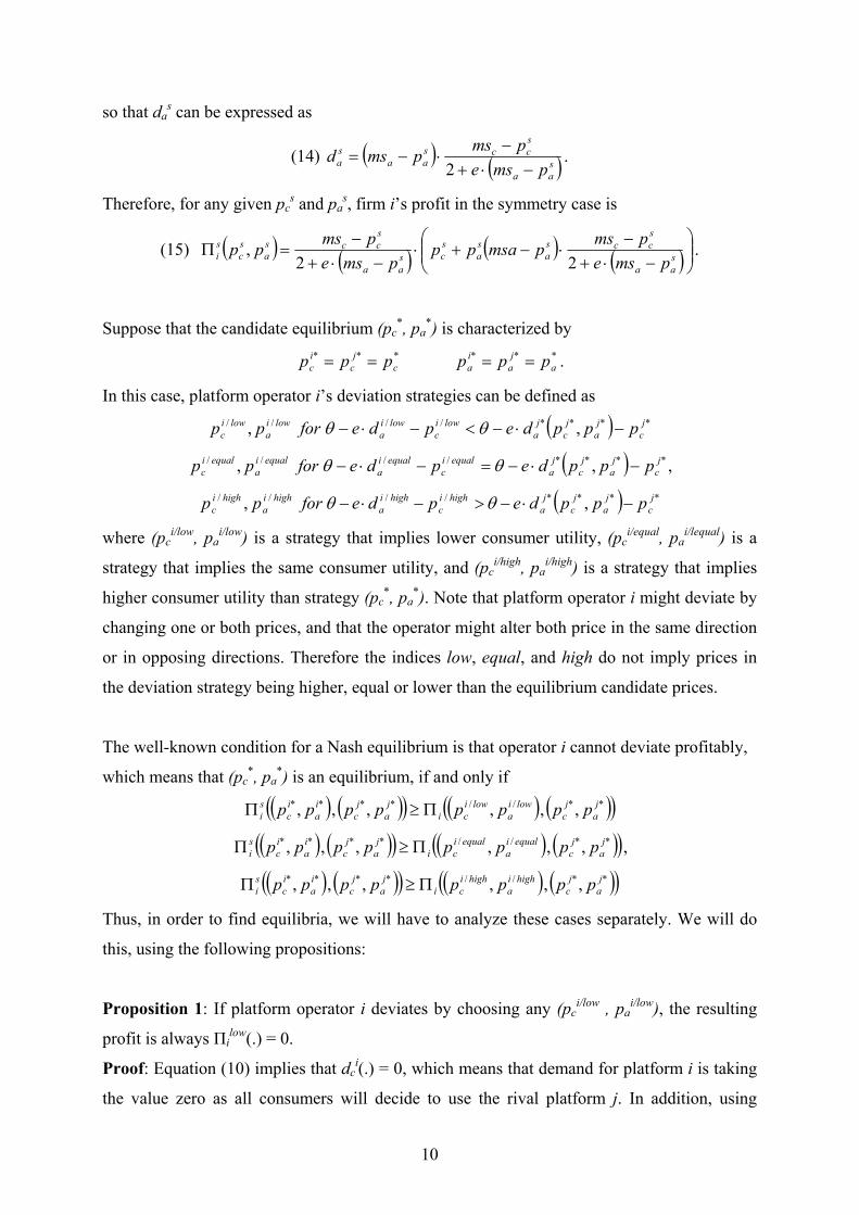
Therefore, for any given pcs and pa

s, firm i’s profit in the symmetry case is

(15) ( ) ( ) ( ) ( )

−⋅+

−⋅−+⋅

−⋅+−

=Πs

aa

s

ccs

a

s

a

s

cs

aa

s

ccs

a

s

c

s

ipmse

pmspmsapp

pmse

pmspp

22, .

Suppose that the candidate equilibrium (pc*, pa

*) is characterized by

***

c

j

c

i

c ppp == ***

a

j

a

i

a ppp == .

In this case, platform operator i’s deviation strategies can be defined as

( ) ****//// ,, j

c

j

a

j

c

j

a

lowi

c

lowi

a

lowi

a

lowi

c pppdepdeforpp −⋅−<−⋅− θθ

( ) ****//// ,, j

c

j

a

j

c

j

a

equali

c

equali

a

equali

a

equali

c pppdepdeforpp −⋅−=−⋅− θθ ,

( ) ****//// ,, j

c

j

a

j

c

j

a

highi

c

highi

a

highi

a

highi

c pppdepdeforpp −⋅−>−⋅− θθ

where (pci/low

, pai/low

) is a strategy that implies lower consumer utility, (pci/equal

, pai/lequal

) is a

strategy that implies the same consumer utility, and (pci/high

, pai/high

) is a strategy that implies

higher consumer utility than strategy (pc*, pa

*). Note that platform operator i might deviate by

changing one or both prices, and that the operator might alter both price in the same direction

or in opposing directions. Therefore the indices low, equal, and high do not imply prices in

the deviation strategy being higher, equal or lower than the equilibrium candidate prices.

The well-known condition for a Nash equilibrium is that operator i cannot deviate profitably,

which means that (pc*, pa

*) is an equilibrium, if and only if

( ) ( )( ) ( ) ( )( )**//**** ,,,,,, j

a

j

c

lowi

a

lowi

ci

j

a

j

c

i

a

i

c

s

i pppppppp Π≥Π

( ) ( )( ) ( ) ( )( )**//**** ,,,,,, j

a

j

c

equali

a

equali

ci

j

a

j

c

i

a

i

c

s

i pppppppp Π≥Π ,

( ) ( )( ) ( ) ( )( )**//**** ,,,,,, j

a

j

c

highi

a

highi

ci

j

a

j

c

i

a

i

c

s

i pppppppp Π≥Π

Thus, in order to find equilibria, we will have to analyze these cases separately. We will do

this, using the following propositions:

Proposition 1: If platform operator i deviates by choosing any (pci/low

, pai/low

), the resulting

profit is always Πilow

(.) = 0.

Proof: Equation (10) implies that dci(.) = 0, which means that demand for platform i is taking

the value zero as all consumers will decide to use the rival platform j. In addition, using

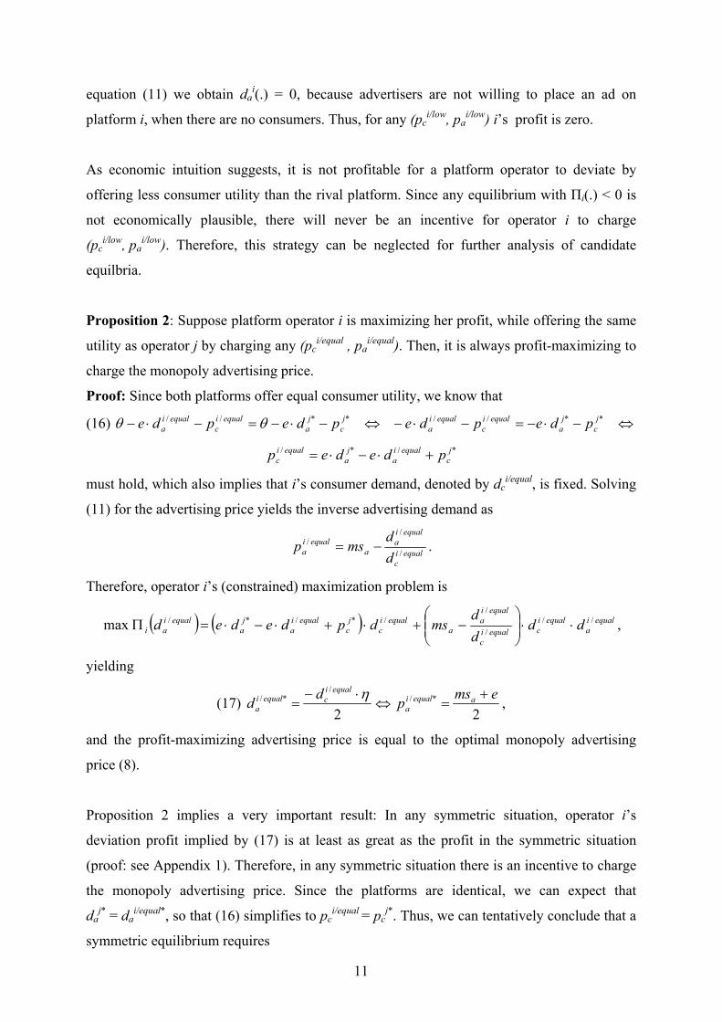
11

equation (11) we obtain dai(.) = 0, because advertisers are not willing to place an ad on

platform i, when there are no consumers. Thus, for any (pci/low

, pai/low

) i’s profit is zero.

As economic intuition suggests, it is not profitable for a platform operator to deviate by

offering less consumer utility than the rival platform. Since any equilibrium with Πi(.) < 0 is

not economically plausible, there will never be an incentive for operator i to charge

(pci/low

, pai/low

). Therefore, this strategy can be neglected for further analysis of candidate

equilbria.

Proposition 2: Suppose platform operator i is maximizing her profit, while offering the same

utility as operator j by charging any (pci/equal

, pai/equal

). Then, it is always profit-maximizing to

charge the monopoly advertising price.

Proof: Since both platforms offer equal consumer utility, we know that

(16) ⇔−⋅−=−⋅−⇔−⋅−=−⋅− **//**// j

c

j

a

equali

c

equali

a

j

c

j

a

equali

c

equali

a pdepdepdepde θθ

*/*/ j

c

equali

a

j

a

equali

c pdedep +⋅−⋅=

must hold, which also implies that i’s consumer demand, denoted by dci/equal

, is fixed. Solving

(11) for the advertising price yields the inverse advertising demand as

equali

c

equali

a

a

equali

ad

dmsp

/

// −= .

Therefore, operator i’s (constrained) maximization problem is

( ) ( ) equali

a

equali

cequali

c

equali

a

a

equali

c

j

c

equali

a

j

a

equali

ai ddd

dmsdpdeded //

/

/

/*/*/max ⋅⋅

−+⋅+⋅−⋅=Π ,

yielding

(17) 22

*//

*/ emsp

dd aequali

a

equali

cequali

a

+=⇔

⋅−=

η,

and the profit-maximizing advertising price is equal to the optimal monopoly advertising

price (8).

Proposition 2 implies a very important result: In any symmetric situation, operator i’s

deviation profit implied by (17) is at least as great as the profit in the symmetric situation

(proof: see Appendix 1). Therefore, in any symmetric situation there is an incentive to charge

the monopoly advertising price. Since the platforms are identical, we can expect that

daj*

= dai/equal*

, so that (16) simplifies to pci/equal

= pcj*

. Thus, we can tentatively conclude that a

symmetric equilibrium requires

12

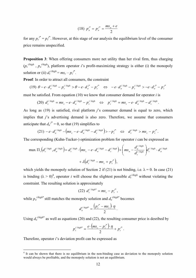
(18) 2

** emspp aj

a

i

a

+==

for any pci*

= pcj*

. However, at this stage of our analysis the equilibrium level of the consumer

price remains unspecified.

Proposition 3: When offering consumers more net utility than her rival firm, thus charging

(pci/high

, pai/high

), platform operator i’s profit-maximizing strategy is either (i) the monopoly

solution or (ii) dci/high

= msc – pcj*

.

Proof: In order to attract all consumers, the constraint

(19) **//**// j

c

j

a

highi

c

highi

a

j

c

j

a

highi

c

highi

a pdepdepdepde −⋅−>−⋅−⇔−⋅−>−⋅− θθ

must be satisfied. From equation (10) we know that consumer demand for operator i is

(20) highi

c

highi

ac

highi

c

highi

c

highi

ac

highi

c ddemsppdemsd ////// −⋅−=⇔−⋅−= .

As long as (19) is satisfied, rival platform j’s consumer demand is equal to zero, which

implies that j’s advertising demand is also zero. Therefore, we assume that consumers

anticipate that da j*

= 0, so that (19) simplifies to

(21) ( ) */*/// j

cc

highi

c

j

c

highi

c

highi

ac

highi

a pmsdpddemsde −>⇔−>−⋅−−⋅− .

The corresponding (Kuhn-Tucker-) optimization problem for operator i can be expressed as

( ) ( ) highi

a

highi

chighi

c

highi

a

a

highi

c

highi

ac

highi

c

highi

a

highi

ci ddd

dmsddemsddd //

/

/

///// ,max ⋅

−+−⋅−⋅=Π

( )*/ j

cc

highi

c pmsd +−+ λ ,

which yields the monopoly solution of Section 2 if (21) is not binding, i.e. λ = 0. In case (21)

is binding (λ > 0)4, operator i will choose the slightest possible dc

i/high without violating the

constraint. The resulting solution is approximately

(22) **/ j

cc

highi

c pmsd −= ,

while pai/high*

still matches the monopoly solution and dai/high*

becomes

( )2

**/ η⋅−= c

j

chighi

a

mspd .

Using dai/high*

as well as equations (20) and (22), the resulting consumer price is desribed by

( ) **

*/

2

j

c

j

cchighi

c ppmse

p +⋅−⋅

=η

.

Therefore, operator i’s deviation profit can be expressed as

4 It can be shown that there is no equilibrium in the non-binding case as deviation to the monopoly solution

would always be profitable, and the monopoly solution is not an equilibrium.

13

(23) ( ) ( ) ( )[ ]**2** 44

1 j

c

j

cc

j

cc

j

c

high

i ppmspmsp ⋅+−⋅⋅−⋅=Π η .

The symmetric equilibrium is characterized by the results of Propositions 2 and 3. As stated

before, Proposition 2 implies that both platform operators charge the monopoly advertising

price in equilibrium, given any consumer price. The equilibrium consumer price can be

obtained by the results of Proposition 3, because there is no incentive for deviation, if the

deviation profit, given by (23), equals the platform’s profit in the symmetry case. Therefore,

in equilibrium

( ) ( )*** , ac

s

ic

high

i ppp Π=Π

must hold. Given (18) and using equations (15) and (23), the equilibrium consumer price5 is

(24) ( )( )[ ]

ζηηη ca

c

msmseep

⋅⋅−−⋅⋅+⋅⋅=

12820 2* , where

( )( )( )[ ] 321281244 2 −⋅−⋅+−⋅+⋅⋅= aa msmsee ηηηζ .

The equilibrium is therefore characterized by (17) and (24), yielding

(25) ( )

ζηη ⋅−⋅⋅⋅

===ems

ddd cj

a

i

aa

24***

(26) ( )ζ

η 2ms8 c*** −⋅⋅⋅===

eddd j

c

i

cc

(27) ( )( )( )( )

2

22*** 24268

ζηηηη −⋅−⋅⋅+−⋅⋅⋅⋅

=Π=Π=Πeemsems acji ,

where an economically plausible symmetric equilibrium solution obviously requires

( ) ( ) ( ) 0,,,,, ****** ≥Π ac

s

aac

s

cac

s

i ppdppdpp .

To obtain economically plausible results, we need to restrict the parameter values as follows:

In case of ad-aversion (e > 0), economically plausible values result for

( ) ( ){ },,0, aaa msemsems ≤≤>∈ α where

α = R2 of ( ) ( ) x6-ms+x-1ms2+2

a

2

a

3 ⋅⋅⋅x .6

5 There is another symmetric equilibrium for pc

* = msc, which generates a corner solution and will be ignored for

the rest of the paper. 6 Rl, l = 1,...,n, denotes the l-th real-valued polynomial root in ascending order of the corresponding polynom of

degree n.

14

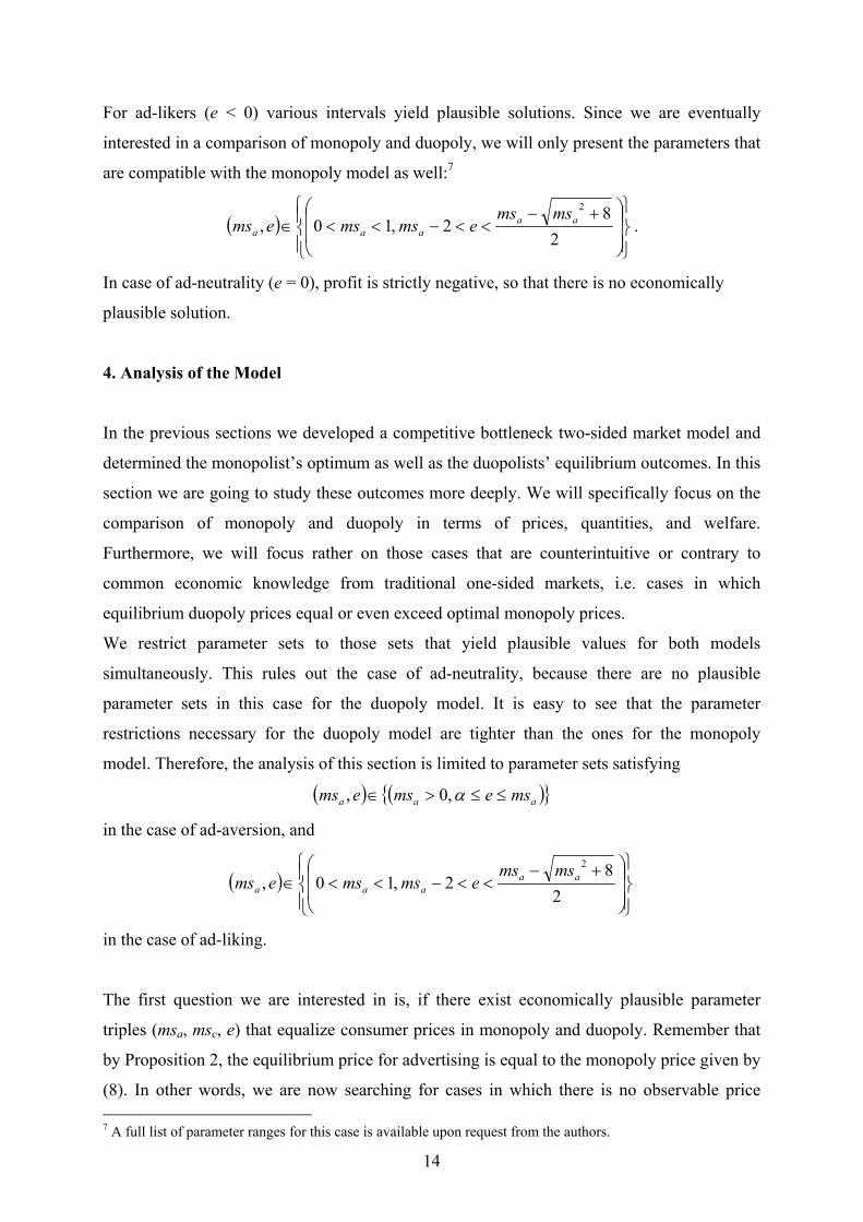
For ad-likers (e < 0) various intervals yield plausible solutions. Since we are eventually

interested in a comparison of monopoly and duopoly, we will only present the parameters that

are compatible with the monopoly model as well:7

( )

+−<<−<<∈

2

82,10,

2

aa

aaa

msmsemsmsems .

In case of ad-neutrality (e = 0), profit is strictly negative, so that there is no economically

plausible solution.

4. Analysis of the Model

In the previous sections we developed a competitive bottleneck two-sided market model and

determined the monopolist’s optimum as well as the duopolists’ equilibrium outcomes. In this

section we are going to study these outcomes more deeply. We will specifically focus on the

comparison of monopoly and duopoly in terms of prices, quantities, and welfare.

Furthermore, we will focus rather on those cases that are counterintuitive or contrary to

common economic knowledge from traditional one-sided markets, i.e. cases in which

equilibrium duopoly prices equal or even exceed optimal monopoly prices.

We restrict parameter sets to those sets that yield plausible values for both models

simultaneously. This rules out the case of ad-neutrality, because there are no plausible

parameter sets in this case for the duopoly model. It is easy to see that the parameter

restrictions necessary for the duopoly model are tighter than the ones for the monopoly

model. Therefore, the analysis of this section is limited to parameter sets satisfying

( ) ( ){ }aaa msemsems ≤≤>∈ α,0,

in the case of ad-aversion, and

( )

+−<<−<<∈

2

82,10,

2

aa

aaa

msmsemsmsems

in the case of ad-liking.

The first question we are interested in is, if there exist economically plausible parameter

triples (msa, msc, e) that equalize consumer prices in monopoly and duopoly. Remember that

by Proposition 2, the equilibrium price for advertising is equal to the monopoly price given by

(8). In other words, we are now searching for cases in which there is no observable price

7 A full list of parameter ranges for this case is available upon request from the authors.

15

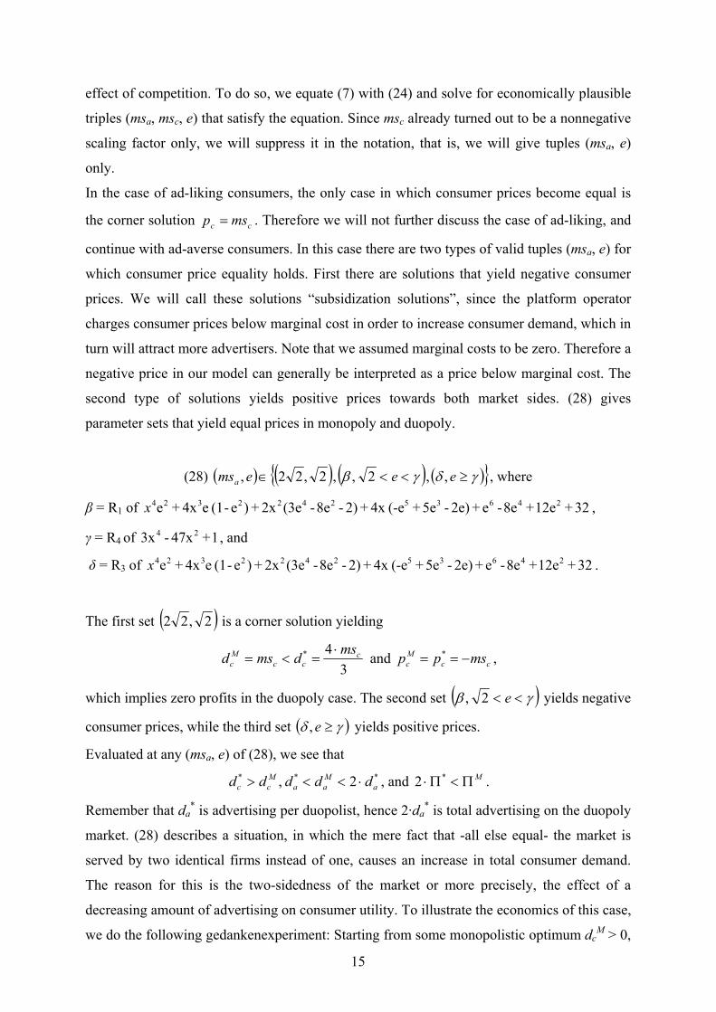
effect of competition. To do so, we equate (7) with (24) and solve for economically plausible

triples (msa, msc, e) that satisfy the equation. Since msc already turned out to be a nonnegative

scaling factor only, we will suppress it in the notation, that is, we will give tuples (msa, e)

only.

In the case of ad-liking consumers, the only case in which consumer prices become equal is

the corner solution cc msp = . Therefore we will not further discuss the case of ad-liking, and

continue with ad-averse consumers. In this case there are two types of valid tuples (msa, e) for

which consumer price equality holds. First there are solutions that yield negative consumer

prices. We will call these solutions “subsidization solutions”, since the platform operator

charges consumer prices below marginal cost in order to increase consumer demand, which in

turn will attract more advertisers. Note that we assumed marginal costs to be zero. Therefore a

negative price in our model can generally be interpreted as a price below marginal cost. The

second type of solutions yields positive prices towards both market sides. (28) gives

parameter sets that yield equal prices in monopoly and duopoly.

(28) ( ) ( ) ( ) ( ){ }γδγβ ≥<<∈ eeemsa ,,2,,2,22, , where

β = R1 of 32+12e+8e-e+2e)-5e+(-e4x +2)-8e-(3e2x+)e-(1 e4x+e 246352422324x ,

γ = R4 of 1+47x-3x 24 , and

δ = R3 of 32+12e+8e-e+2e)-5e+(-e4x +2)-8e-(3e2x+)e-(1 e4x+e 246352422324x .

The first set ( )2,22 is a corner solution yielding

3

4* ccc

M

c

msdmsd

⋅=<= and cc

M

c mspp −== * ,

which implies zero profits in the duopoly case. The second set ( )γβ << e2, yields negative

consumer prices, while the third set ( )γδ ≥e, yields positive prices.

Evaluated at any (msa, e) of (28), we see that

*** 2, a

M

aa

M

cc ddddd ⋅<<> , and MΠ<Π⋅ *2 .

Remember that da* is advertising per duopolist, hence 2·da

* is total advertising on the duopoly

market. (28) describes a situation, in which the mere fact that -all else equal- the market is

served by two identical firms instead of one, causes an increase in total consumer demand.

The reason for this is the two-sidedness of the market or more precisely, the effect of a

decreasing amount of advertising on consumer utility. To illustrate the economics of this case,

we do the following gedankenexperiment: Starting from some monopolistic optimum dcM

> 0,

16

daM

> 0, we imagine that -all else equal- the monopolist is replaced by two identical, but

independent platforms. In this case, total consumer demand dcM

will be equally divided

among the two platforms. As a consquence, advertising with one platform only reaches half

of the consumers, which will reduce advertising demand per platform to some dan < da

M.

Since we assumed e > 0, the decrease in advertising exposure increases total consumer

demand to some dcn > dc

M. This increase in consumer demand in turn increases advertising

demand. However, eventually the increase does not offset the decreasing effect, so that the

total effect on advertising per platform is negative, from which follows that the total effect on

consumer demand is positive.

The follow-up question to the results established above is, whether duopoly equilibrium

consumer prices might even exceed optimal monopoly consumer prices. Again, we only need

to consider the case of ad-aversion, since there is no parameter set that creates this effect if

consumers are ad-likers. As before, there are subsidization solutions and solutions with

positive prices. However, it is now also possible that the monopolist charges negative

consumer prices, while the duopolists do not. In the case of subsidization, less negative prices

in the duopoly case can be interpreted as a lower subsidization of consumers as compared to

the monopoly case. (29) describes parameter sets given which the duopoly equilibrium

consumer price exceeds the optimal monopoly consumer price.

(29) ( )

≥

+⋅+−≤<

<

+⋅+−≤<∈ γδγβ e

e

eems

e

eemsems aaa ,

141,e<2,

141,

2222

Evaluated at any (msa, e) of (29), we see that

MΠ<Π⋅ *2 and M

aa dd <* ,

which is so far consistent with the results obtained from (28). However, we cannot draw

general conclusions about the relationship of *

cd and M

cd , and of M

ad and *2 ad .

Refining (29) for those solutions that yield negative consumer prices, we obtain

(30) ( )

>

+⋅+−≤<

≤

+⋅+−≤<

∈

κω

κβ

ee

eems

e

eems

ems

a

a

a

,141

,e<2,141

,22

22

, where

κ = R2 of 36-32x+10x-x 246 , and

ω = R1 of 20e-8e+e-)x3e+16e-(12+)x3e-(8e+xe 35522332 .

17

In case

≤

+⋅+−≤< κβ e<2,

141 22

e

eemsa ,

M

aa dd >⋅ *2 and M

cc dd >* hold, while for

>

+⋅+−≤< κω e

e

eemsa ,

141 22

the relationships of *

cd and M

cd and M

ad and *2 ad⋅ are still ambigous.

Parameter sets that yield a mixed case, in which a monopolist will subsidize while the

duopolists will not, are described by (31).

(31) ( )

>≤<

++∈ κδ ems

eeems aa ,

2

8,

2

The results in case of (31) are analogue to the results of the second solution of (30): da* < da

M

and 2·П* < ПM

hold, while the relationship of dc* and dc

M as well as da

M and 2·da

* is ambigous.

Positive prices result, if

(32) ( )

>

++<<

<<

++<<∈ βδγκβ e

eemse

eemsems aaa ,

2

8,,

2

8,

22

.

For both solutions of (32) it holds that *** 2, a

M

aa

M

cc ddddd <<> , and MΠ<Π⋅ *2 .

Table 1 summarizes the results.

Case *

cd ⋛ M

cd *

ad ⋛ M

ad *2 ad ⋛ M

ad *2 Π⋅ ⋛ MΠ

Subsidization > < > < M

cc pp =*

Positive Prices > < > <

Subsidization 1 > < > <

Subsidization 2 ⋛ < ⋛ <

Mixed ⋛ < ⋛ <

M

cc pp >*

Positive Prices > < > <

Table 1: Relationship of quantities and profits, if consumer prices are equal or if the duopoly

consumer price exceeds the monopoly consumer price.

18

Most notably, even though prices in the monopoly are not higher than in duopoly, monopoly

profit still is strictly greater than total profit in the duopoly. This is in line with Chaudhri

(1998), who compares monopoly and perfectly competitive newspaper markets, and finds that

“(u)pon attaining monopoly control of a newspaper market, a proprietor, for reasonable

parameter values […] opts to lower the price for her newspaper, which increases circulation,

and hence, increased advertising revenue” (p.74).

Finally, we will study the welfare effects imposed by our model. Since we assumed zero costs

of production, monopoly profit, resp. the sum of both provider’s profits is equal to producer

surplus. Traditional “consumer surplus” here is the sum of the surplus created on both market

sides. In the monopoly case, the market side we labeled “consumers” realizes a benefit of

( ) ( )220 4

2,

−

⋅=⋅−∫ η

cM

c

M

cc

d

M

ac

M

c

mspdddddp

Mc

,

where M

cd is given by (5), M

ad is given by (6), M

cp is given by (7), and ( )⋅M

cp is the inverse

of (2). In the duopoly case the consumer side realizes a surplus of

( ) ( )2

22

**

2

0

* 21282,

ζη c

ccc

d

ac

d

c

msepdddddp

ic ⋅⋅−⋅

=⋅−∫ ,

where *

cd is given by (26), *

ad is given by (25), *

cp is given by (24), and ( )⋅d

cp is the inverse

of (13). Advertisers obtain a surplus of

( ) ( )2

2

044

,η

η−⋅⋅

=⋅−∫ cM

a

M

aa

d

M

ca

M

a

mspdddddp

Ma

,

where M

cd is given by (5), M

ad is given by (6), M

ap is given by (8), and ( )⋅M

ap is the inverse

of (4) in the monopoly case, and

( ) ( )ζηη c

aaa

d

ca

d

a

msepdddddp

a ⋅−⋅⋅⋅=

⋅−⋅ ∫

22,2

2**

0

*

*

in the duopoly case, where *

cd is given by (26), *

ad is given by (25), M

aa pp =* is given by (8),

and ( )⋅d

ap is the inverse of (12).

Welfare is given by the sum of producer, consumer, and advertiser surplus. Table 2

summarizes the relation of total welfare in monopoly optimum and duopoly equilibrium as

well as the relations of the individual welfare components.

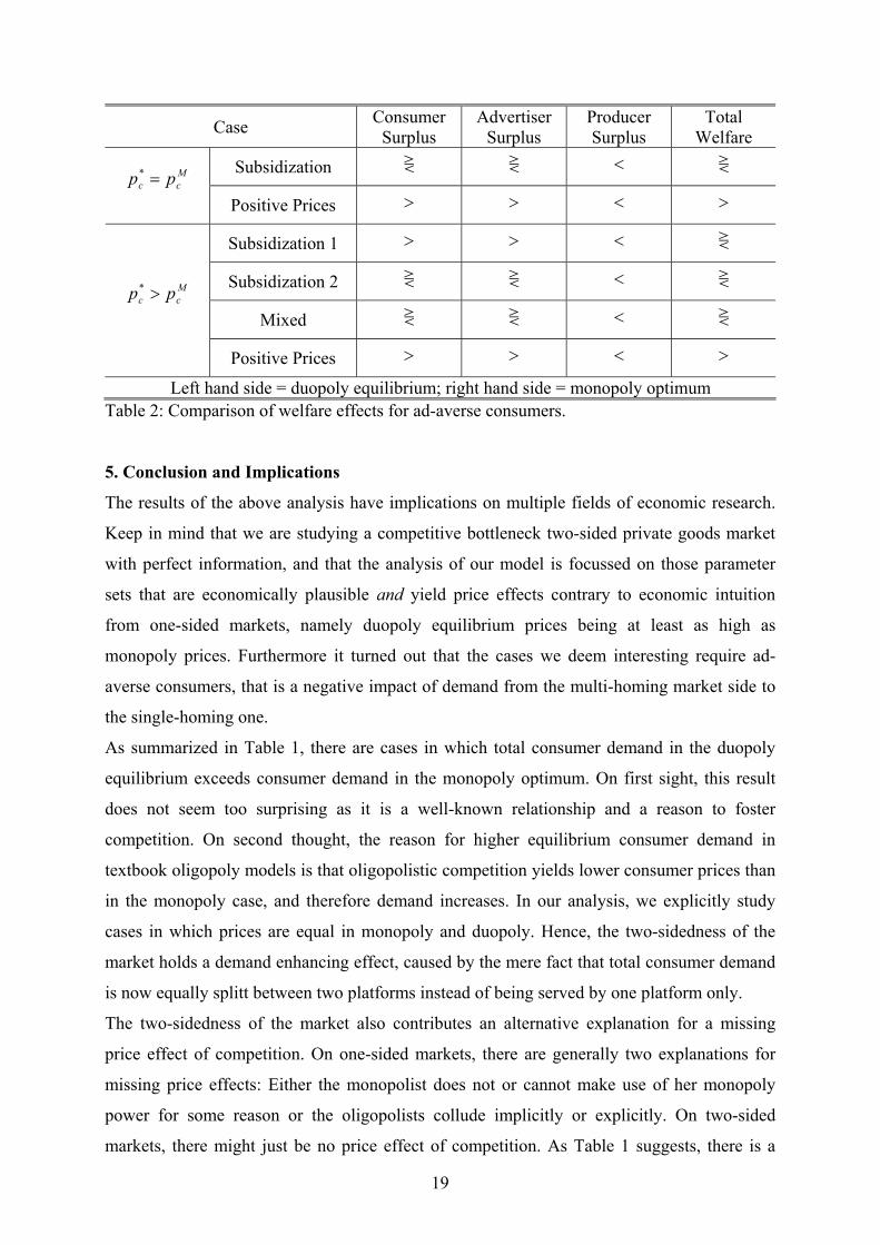
19

Case Consumer

Surplus

Advertiser

Surplus

Producer

Surplus

Total

Welfare

Subsidization ⋛ ⋛ < ⋛ M

cc pp =*

Positive Prices > > < >

Subsidization 1 > > < ⋛

Subsidization 2 ⋛ ⋛ < ⋛

Mixed ⋛ ⋛ < ⋛

M

cc pp >*

Positive Prices > > < >

Left hand side = duopoly equilibrium; right hand side = monopoly optimum

Table 2: Comparison of welfare effects for ad-averse consumers.

5. Conclusion and Implications

The results of the above analysis have implications on multiple fields of economic research.

Keep in mind that we are studying a competitive bottleneck two-sided private goods market

with perfect information, and that the analysis of our model is focussed on those parameter

sets that are economically plausible and yield price effects contrary to economic intuition

from one-sided markets, namely duopoly equilibrium prices being at least as high as

monopoly prices. Furthermore it turned out that the cases we deem interesting require ad-

averse consumers, that is a negative impact of demand from the multi-homing market side to

the single-homing one.

As summarized in Table 1, there are cases in which total consumer demand in the duopoly

equilibrium exceeds consumer demand in the monopoly optimum. On first sight, this result

does not seem too surprising as it is a well-known relationship and a reason to foster

competition. On second thought, the reason for higher equilibrium consumer demand in

textbook oligopoly models is that oligopolistic competition yields lower consumer prices than

in the monopoly case, and therefore demand increases. In our analysis, we explicitly study

cases in which prices are equal in monopoly and duopoly. Hence, the two-sidedness of the

market holds a demand enhancing effect, caused by the mere fact that total consumer demand

is now equally splitt between two platforms instead of being served by one platform only.

The two-sidedness of the market also contributes an alternative explanation for a missing

price effect of competition. On one-sided markets, there are generally two explanations for

missing price effects: Either the monopolist does not or cannot make use of her monopoly

power for some reason or the oligopolists collude implicitly or explicitly. On two-sided

markets, there might just be no price effect of competition. As Table 1 suggests, there is a

20

competitive effect that causes total profits in the duopoly equilibrium to be strictly lower than

in the monopoly case, and total advertising demand to be lower in monopoly than in duopoly.

We neither restrict the monopolist’s optimization problem artificially nor do we hinder

competition between the duopolists. Still and regardless of competition taking place, there is

no observable price effect, given any of the parameter sets described by (28), and competition

even increases prices given any of the parameter sets described by (29)-(32).

A price effect of competition, however, is the underlying assumption of empirical price-

concentration studies. These studies presume that prices increase with the concentration of the

market, and try to estimate the magnitude of this effect. Our results suggest that this

relationship might be negative, given certain exogenous conditions as described by (29)-(32).

Therefore, empirical analyses yielding a negative price-concentration effect, e.g. in the movie

theater industry, do not necessarily suffer from methodological or technological mistakes. If,

however, the exogenous conditions are in such a way as described by (28), then there is

obviously no price effect of competition that could be measured. This implies that the absence

of significant empirical results cannot be interpreted as lack of competition, unless it is

verified that none of the parameter sets of (28) is present in the industry under consideration.

In this light, it is also not sensible to follow Weyl (2006) and study the sum of the prices,

which he calls the “price level”, instead of the “price balance” that describes the relation of

the prices of the two market sides.

Regarding the welfare effects of competition, we obtain ambigous results and need to

distinguish our conclusions by the price level as in Table 2. In case of positive prices, i.e. in

case of prices above marginal cost, total welfare is always higher in the duopoly equilibrium

than in the monopoly optimum, even though consumer prices might be lower under

monopoly. In case of subsidization, this is not necessarily true. Therefore, policy makers as

well as regulators aiming at welfare maximization will have to obtain in-dept knowledge of

the environment (i.e. the parameter set) they are facing before being able to act optimally. A

brief glance at the prevailing price level or price balance will not suffice to make a sensible

judgement. Unlike on common one-sided markets, fostering competition will not necessarily

increase welfare. Similarly, merger control becomes more difficult. Under conditions of

positive prices, mergers generally have a negative impact on total welfare. Under conditions

of subsidized consumer prices, we cannot draw general conclusions. If, for some exogenous

reason, a merger has to take place anyway, it will virtually always imply that one platform

closes down (proof: see Appendix 2). This is in line with the regulator’s objective of welfare

21

maximization, because welfare increases, if the operator of the two merged platforms closes

down one of them. It even holds for distributive objectives, i.e. consumer surplus, advertiser

surplus, and producer surplus all increase, if the operator closes down one platform in case of

a merger (see also Appendix 2).

References

Anderson, S. P., & Gabszewicz, J. J. (2006). The media and advertising: a tale of two-sided

markets. In V. A. Ginsburgh & D. Throsby (Eds.), Handbook of the economics of art

and culture. North-Holland: Elsevier.

Armstrong, M. (2006). Competition in two-sided markets. RAND Journal of Economics,

37(3), 668-691.

Caillaud, B., & Jullien, B. (2003). Chicken & egg: competition among intermediation service

providers. RAND Journal of Economics, 34(2), 309-328.

Chaudhri, V. (1998). Pricing and efficiency of a circulation industry: The case of newspapers.

Information Economics and Policy, 10(1), 59-76.

Danaher, P. J. (1995). What happens to television ratings during commercial breaks? Journal

of Advertising Research, 37(1), 37-47.

Dewenter, R. (2006). Das Konzept der zweiseitigen Märkte am Beispiel von

Zeitungsmonopolen. Hamburg: Department of Economics, Helmut-Schmidt-

University of the Federal Armed Forces.

Gabszewicz, J. J., Laussel, D., & Sonnac, N. (1999). TV-broadcasting competition and

advertising: Centre de Recherche en Economie et Statistique, Université Catholique de

Louvain.

Häckner, J., & Nyberg, S. (2008). Advertising and media market concentration. Journal of

Media Economics, 21(2), 79-96.

Kaiser, U., & Song, M. (2009). Do media consumers really dislike advertising? An empirical

assessment of the role of advertising in print media markets. International Journal of

Industrial Organization, 27(2), 292-301.

Nilssen, T., & Sørgard, L. (2001). The TV industry: advertising and programming. Oslo:

Department of Economics, University of Oslo.

Picard, R. G. (1989). Media economics. Concepts and issues. Newbury Park, London, New

Delhi: Sage.

Rochet, J.-C., & Tirole, J. (2003). Platform competition in two-sided markets. Journal of the

European Economic Association, 1(4), 990-1029.

Rysman, M. (2004). Competition between networks: a study of the market for yellow pages.

Review of Economic Studies, 71(2), 483-512.

Weyl, E. G. (2006). The price theory of two-sided markets. Princeton: Bendheim Center for

Finance, Department of Economics, Princeton University.

Wilbur, K. C. (2007). A two-sided, empirical model of television advertising and viewing

markets. Los Angeles: University of Southern California.

22

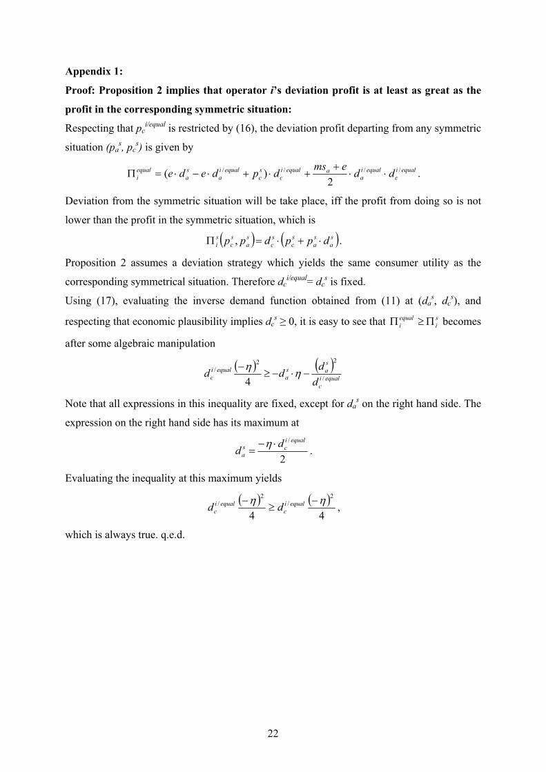
Appendix 1:

Proof: Proposition 2 implies that operator i’s deviation profit is at least as great as the

profit in the corresponding symmetric situation:

Respecting that pci/equal

is restricted by (16), the deviation profit departing from any symmetric

situation (pas, pc

s) is given by

equali

c

equali

aaequali

c

s

c

equali

a

s

a

equal

i ddems

dpdede ////

2)( ⋅⋅

++⋅+⋅−⋅=Π .

Deviation from the symmetric situation will be take place, iff the profit from doing so is not

lower than the profit in the symmetric situation, which is

( ) ( )s

a

s

a

s

c

s

c

s

a

s

c

s

i dppdpp ⋅+⋅=Π , .

Proposition 2 assumes a deviation strategy which yields the same consumer utility as the

corresponding symmetrical situation. Therefore dci/equal

= dcs is fixed.

Using (17), evaluating the inverse demand function obtained from (11) at (das, dc

s), and

respecting that economic plausibility implies dcs ≥ 0, it is easy to see that s

i

equal

i Π≥Π becomes

after some algebraic manipulation

( ) ( )equali

c

s

as

a

equali

cd

ddd

/

22

/

4−⋅−≥

− ηη

Note that all expressions in this inequality are fixed, except for das on the right hand side. The

expression on the right hand side has its maximum at

2

/ equali

cs

a

dd

⋅−=

η.

Evaluating the inequality at this maximum yields

( ) ( )44

2

/

2

/ ηη −≥

− equali

c

equali

c dd ,

which is always true. q.e.d.

23

Appendix 2:

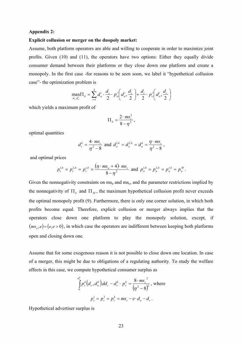
Explicit collusion or merger on the duopoly market:

Assume, both platform operators are able and willing to cooperate in order to maximize joint

profits. Given (10) and (11), the operators have two options: Either they equally divide

consumer demand between their platforms or they close down one platform and create a

monopoly. In the first case -for reasons to be seen soon, we label it “hypothetical collusion

case”- the optimization problem is

∑=

⋅+

⋅⋅=Π

2

1, 2

,22

,2

maxi

ci

a

i

ccci

a

i

aci

akdd

ddp

dddp

dd

iac

which yields a maximum profit of

2

2

8

2

η−⋅

=Π ck

ms,

optimal quantities

8

42 −⋅

=η

ck

c

msd and

82

,2,1

−⋅

===ηη ck

a

k

a

k

a

msddd ,

and optimal prices

( )2

,,2,1

8

4

ηη

−⋅+⋅

=== caki

c

k

c

k

c

msmsppp and M

a

ki

a

k

a

k

a pppp === ,,2,1 .

Given the nonnegativity constraints on msa and msc, and the parameter restrictions implied by

the nonnegativity of kΠ and MΠ , the maximum hypothetical collusion profit never exceeds

the optimal monopoly profit (9). Furthermore, there is only one corner solution, in which both

profits become equal. Therefore, explicit collusion or merger always implies that the

operators close down one platform to play the monopoly solution, except, if

( ) ( )0,, >= eeemsa, in which case the operators are indifferent between keeping both platforms

open and closing down one.

Assume that for some exogenous reason it is not possible to close down one location. In case

of a merger, this might be due to obligations of a regulating authority. To study the welfare

effects in this case, we compute hypothetical consumer surplus as

( ) ( )22

2

0 8

8,

−

⋅=⋅−∫ η

ck

c

k

cc

d

k

ac

k

c

mspdddddp

kc

, where

cac

k

ccc ddemsppp −⋅−=== 21 .

Hypothetical advertiser surplus is

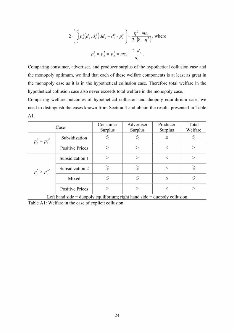
24

( ) ( )2

2

082

,2η

η−⋅⋅

=

⋅−⋅ ∫ ck

a

k

aa

d

k

ca

k

a

mspdddddp

ka

, where

c

aa

k

aaad

dmsppp

⋅−===

221 .

Comparing consumer, advertiser, and producer surplus of the hypothetical collusion case and

the monopoly optimum, we find that each of these welfare components is at least as great in

the monopoly case as it is in the hypothetical collusion case. Therefore total welfare in the

hypothetical collusion case also never exceeds total welfare in the monopoly case.

Comparing welfare outcomes of hypothetical collusion and duopoly equilibrium case, we

need to distinguish the cases known from Section 4 and obtain the results presented in Table

A1.

Case Consumer

Surplus

Advertiser

Surplus

Producer

Surplus

Total

Welfare

Subsidization ⋛ ⋛ ≤ ⋛ M

cc pp =*

Positive Prices > > < >

Subsidization 1 > > < >

Subsidization 2 ⋛ ⋛ ≤ ⋛

Mixed ⋛ ⋛ ≤ ⋛

M

cc pp >*

Positive Prices > > < >

Left hand side = duopoly equilibrium; right hand side = duopoly collusion

Table A1: Welfare in the case of explicit collusion