comparing observed and theoretical distributions - … · maarten l. buis comparing observed and...
TRANSCRIPT

Univariate distributionsMarginal distributions
Comparing observed and theoreticaldistributions
Maarten L. Buis
Institut für SoziologieEberhard Karls Universität Tübingen
www.maartenbuis.nl
Maarten L. Buis Comparing observed and theoretical distributions
Univariate distributionsMarginal distributions
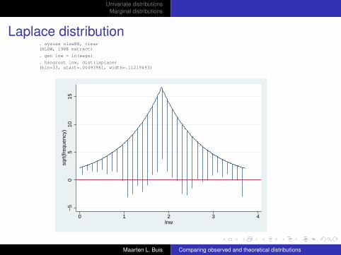
Laplace distribution. sysuse nlsw88, clear(NLSW, 1988 extract)
. gen lnw = ln(wage)
. hangroot lnw, dist(laplace)(bin=33, start=.00493961, width=.11219493)
−5
05
1015
sqrt
(fre
quen
cy)
0 1 2 3 4lnw
Maarten L. Buis Comparing observed and theoretical distributions
Univariate distributionsMarginal distributions
Introduction
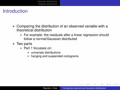
I Comparing the distribution of an observed variable with atheoretical distribution
I For example: the residuals after a linear regression shouldfollow a normal/Gaussian distributed
I Two partsI Part 1 focusses on:
I univariate distributionsI hanging and suspended rootograms
I Part 2 focusses on:I marginal distributionsI hanging and suspend rootograms and pp and qq-plots
Maarten L. Buis Comparing observed and theoretical distributions

Univariate distributionsMarginal distributions
Introduction
I Comparing the distribution of an observed variable with atheoretical distribution
I For example: the residuals after a linear regression shouldfollow a normal/Gaussian distributed
I Two partsI Part 1 focusses on:
I univariate distributionsI hanging and suspended rootograms
I Part 2 focusses on:I marginal distributionsI hanging and suspend rootograms and pp and qq-plots
Maarten L. Buis Comparing observed and theoretical distributions

Univariate distributionsMarginal distributions
Outline
Univariate distributions
Marginal distributions
Maarten L. Buis Comparing observed and theoretical distributions

Univariate distributionsMarginal distributions
histogram with normal curve
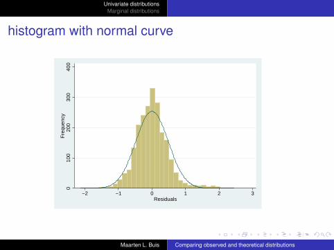
. sysuse nlsw88, clear(NLSW, 1988 extract)
. gen ln_w = ln(wage)
. reg ln_w grade age ttl_exp tenure
Source SS df MS Number of obs = 2229F( 4, 2224) = 214.79
Model 203.980816 4 50.9952039 Prob > F = 0.0000Residual 528.026987 2224 .237422206 R-squared = 0.2787
Adj R-squared = 0.2774Total 732.007802 2228 .328549283 Root MSE = .48726
ln_w Coef. Std. Err. t P>|t| [95% Conf. Interval]
grade .0798009 .0041795 19.09 0.000 .0716048 .087997age -.009702 .0034036 -2.85 0.004 -.0163765 -.0030274
ttl_exp .0312377 .0027926 11.19 0.000 .0257613 .0367141tenure .0121393 .0022939 5.29 0.000 .0076408 .0166378_cons .7426107 .1447075 5.13 0.000 .4588348 1.026387
. predict resid, resid(17 missing values generated)
. hist resid, normal freq(bin=33, start=-2.1347053, width=.13879342)
Maarten L. Buis Comparing observed and theoretical distributions
Univariate distributionsMarginal distributions
histogram with normal curve
010
020
030
040
0F
requ
ency
−2 −1 0 1 2 3Residuals
Maarten L. Buis Comparing observed and theoretical distributions

Univariate distributionsMarginal distributions
hanging rootogram, Tukey 1972 and 1977
. hangroot resid(bin=33, start=-2.1347053, width=.13879342)
010
020
030
040
0F
requ
ency
−2 −1 0 1 2 3Residuals
−5
05
1015
sqrt
(fre
quen
cy)
−2 −1 0 1 2 3Residuals
Maarten L. Buis Comparing observed and theoretical distributions
Univariate distributionsMarginal distributions
Confidence intervalsI For a histogram the variable is broken up in a number of
bins.
I The hight of a bar/spike is the number of observationsfalling in a bin.
I One can think of this number of observations as following amultinomial distribution.
I Confidence intervals for these counts are computed usingGoodman’s (1965) approximation of the simultaneousconfidence interval.
I For (hanging) rootograms these confidence intervals aretransformed to the square root scale.
I These confidence intervals do not take into account that:I the parameters of the theoretical curve are often estimatedI and that nearby bins are often similar.
Maarten L. Buis Comparing observed and theoretical distributions

Univariate distributionsMarginal distributions
Confidence intervalsI For a histogram the variable is broken up in a number of
bins.I The hight of a bar/spike is the number of observations
falling in a bin.
I One can think of this number of observations as following amultinomial distribution.
I Confidence intervals for these counts are computed usingGoodman’s (1965) approximation of the simultaneousconfidence interval.
I For (hanging) rootograms these confidence intervals aretransformed to the square root scale.
I These confidence intervals do not take into account that:I the parameters of the theoretical curve are often estimatedI and that nearby bins are often similar.
Maarten L. Buis Comparing observed and theoretical distributions

Univariate distributionsMarginal distributions
Confidence intervalsI For a histogram the variable is broken up in a number of
bins.I The hight of a bar/spike is the number of observations
falling in a bin.I One can think of this number of observations as following a
multinomial distribution.
I Confidence intervals for these counts are computed usingGoodman’s (1965) approximation of the simultaneousconfidence interval.
I For (hanging) rootograms these confidence intervals aretransformed to the square root scale.
I These confidence intervals do not take into account that:I the parameters of the theoretical curve are often estimatedI and that nearby bins are often similar.
Maarten L. Buis Comparing observed and theoretical distributions
Univariate distributionsMarginal distributions
Confidence intervalsI For a histogram the variable is broken up in a number of
bins.I The hight of a bar/spike is the number of observations
falling in a bin.I One can think of this number of observations as following a
multinomial distribution.I Confidence intervals for these counts are computed using
Goodman’s (1965) approximation of the simultaneousconfidence interval.
I For (hanging) rootograms these confidence intervals aretransformed to the square root scale.
I These confidence intervals do not take into account that:I the parameters of the theoretical curve are often estimatedI and that nearby bins are often similar.
Maarten L. Buis Comparing observed and theoretical distributions

Univariate distributionsMarginal distributions
Confidence intervals. hangroot resid, ci(bin=33, start=-2.1347053, width=.13879342)
−5
05
1015
sqrt
(fre
quen
cy)
−2 −1 0 1 2 3Residuals
95% Conf. Int.
Maarten L. Buis Comparing observed and theoretical distributions
Univariate distributionsMarginal distributions
Simulations
I We know that the residuals should follow a normaldistribution with mean 0 and standard deviation e(rmse).
I We can compare the observed distribution with severaldraws from this theoretical distribution.
I The simulated distributions capture the variability one canexpect if our model is true
Maarten L. Buis Comparing observed and theoretical distributions

Univariate distributionsMarginal distributions
Simulations. forvalues i = 1/20 {
2. qui gen sim`i´ = rnormal(0,`e(rmse)´) if e(sample)3. }
. hangroot resid, sims(sim*) jitter(5)(bin=34, start=-2.1347053, width=.13471126)
−5
05
1015
sqrt
(fre
quen
cy)
−2 −1 0 1 2 3Residuals
observed simulations
Maarten L. Buis Comparing observed and theoretical distributions

Univariate distributionsMarginal distributions
Suspended rootogram. hangroot resid, ci susp theoropt(lpattern(-))(bin=33, start=-2.1347053, width=.13879342)
−15
−10
−5
05
sqrt
(fre
quen
cy)
−2 −1 0 1 2 3Residuals
95% Conf. Int. residual
Maarten L. Buis Comparing observed and theoretical distributions

Univariate distributionsMarginal distributions
Suspended rootogram. hangroot resid, ci susp notheor(bin=33, start=-2.1347053, width=.13879342)
−2
−1
01
23
sqrt
(res
idua
ls)
−2 −1 0 1 2 3Residuals
95% Conf. Int. residual
Maarten L. Buis Comparing observed and theoretical distributions
Univariate distributionsMarginal distributions
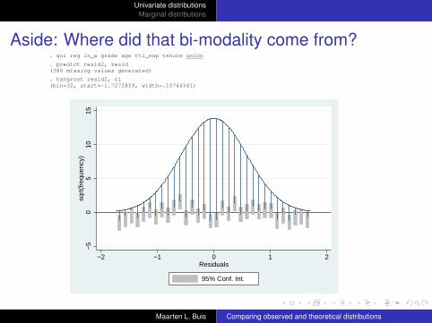
Aside: Where did that bi-modality come from?. qui reg ln_w grade age ttl_exp tenure union
. predict resid2, resid(380 missing values generated)
. hangroot resid2, ci(bin=32, start=-1.7272859, width=.10744561)
−5
05
1015
sqrt
(fre
quen
cy)
−2 −1 0 1 2Residuals
95% Conf. Int.
Maarten L. Buis Comparing observed and theoretical distributions
Univariate distributionsMarginal distributions
Where did the parameters come from?
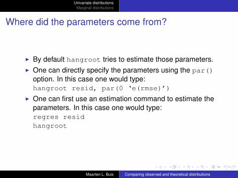
I By default hangroot tries to estimate those parameters.
I One can directly specify the parameters using the par()option. In this case one would type:hangroot resid, par(0 ‘e(rmse)’)
I One can first use an estimation command to estimate theparameters. In this case one would type:regres residhangroot
Maarten L. Buis Comparing observed and theoretical distributions

Univariate distributionsMarginal distributions
Where did the parameters come from?
I By default hangroot tries to estimate those parameters.I One can directly specify the parameters using the par()
option. In this case one would type:hangroot resid, par(0 ‘e(rmse)’)
I One can first use an estimation command to estimate theparameters. In this case one would type:regres residhangroot
Maarten L. Buis Comparing observed and theoretical distributions

Univariate distributionsMarginal distributions
Is this just for the normal distribution?
One can specify other distributions with the dist() option.normal / Gaussian Singh-Maddalalognormal Generalized Beta IIlogistic generalized extreme valueWeibull exponentialChi square Laplacegamma uniformGumbel geometricinverse gamma PoissonWald / inverse Gaussian zero inflated Poissonbeta negative binomial IPareto negative binomial IIFisk / log-logistic zero inflated negative binomialDagum
Maarten L. Buis Comparing observed and theoretical distributions

Univariate distributionsMarginal distributions
Other examples: a beta distribution. use "`home´\citybudget", clear(Spending on different categories by Dutch cities in 2005)
. hangroot governing, dist(beta)(bin=19, start=.02759536, width=.01572787)
−2
02
46
8sq
rt(f
requ
ency
)
0 .1 .2 .3 .4proportion budget spent on governing
Maarten L. Buis Comparing observed and theoretical distributions
Univariate distributionsMarginal distributions
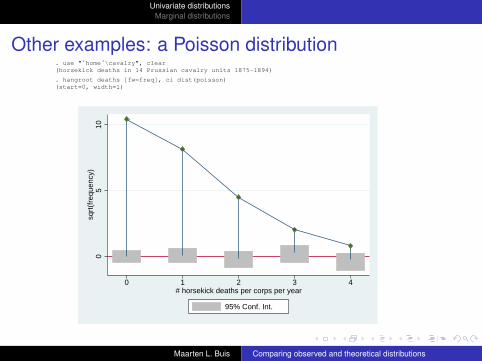
Other examples: a Poisson distribution. use "`home´\cavalry", clear(horsekick deaths in 14 Prussian cavalry units 1875-1894)
. hangroot deaths [fw=freq], ci dist(poisson)(start=0, width=1)
05
10sq
rt(f
requ
ency
)
0 1 2 3 4# horsekick deaths per corps per year
95% Conf. Int.
Maarten L. Buis Comparing observed and theoretical distributions

Univariate distributionsMarginal distributions
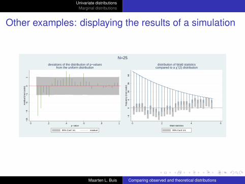
Other examples: displaying the results of a simulation
. program drop _all
. program define sim, rclass1. drop _all2. set obs 2503. gen x1 = rnormal()4. gen x2 = rnormal()5. gen x3 = rnormal()6. gen y = runiform() < invlogit(-2 + x1)7. logit y x1 x2 x38. test x2=x3=09. return scalar p_250 = r(p)10. return scalar chi2_250 = r(chi2)11. logit y x1 x2 x3 in 1/2512. test x2=x3=013. return scalar p_25 = r(p)14. return scalar chi2_25 = r(chi2)15.. end
.
. set seed 123456
.
. simulate chi2_250=r(chi2_250) p_250=r(p_250) ///> chi2_25 =r(chi2_25) p_25 =r(p_25) , ///> reps(1000) nodots : sim
command: simchi2_250: r(chi2_250)
p_250: r(p_250)chi2_25: r(chi2_25)
p_25: r(p_25)
Maarten L. Buis Comparing observed and theoretical distributions

Univariate distributionsMarginal distributions
Other examples: displaying the results of a simulation
. hangroot chi2_25, dist(chi2) par(2) name(chi, replace) ci ///> title("distribution of Wald statistics" ///> "compared to a {&chi}{sup:2}(2) distribution" ) ///> xtitle(Wald statistics) ///> ytitle("frequency (root scale)") ///> ylab(-2 "-4" 0 "0" 2 "4" 4 "16" 6 "36" 8 "64")(bin=29, start=.00226492, width=.18900082)
.
. hangroot p_25 , dist(uniform) par(0 1) ///> susp notheor ci name(p, replace) ///> title("deviations of the distribution of p-values" ///> "from the uniform distribution") ///> xtitle("p-value") ytitle("residual (root scale)") ///> ylab(-4 "-16" -3 "-9" -2 "-4" -1 "-1" 0 "0" 1 "1" )(bin=29, start=.06446426, width=.03222082)
Maarten L. Buis Comparing observed and theoretical distributions

Univariate distributionsMarginal distributions
Other examples: displaying the results of a simulation
. hangroot chi2_250, dist(chi2) par(2) name(chi2, replace) ci ///> title("distribution of Wald statistics" ///> "compared to a {&chi}{sup:2}(2) distribution" ) ///> xtitle(Wald statistics) ///> ytitle("frequency (root scale)") ///> ylab(-5 "-25" 0 "0" 5 "25" 10 "100" 15 "225" )(bin=29, start=.00158109, width=.41837189)
.
. hangroot p_250 , dist(uniform) par(0 1) ///> susp notheor ci name(p2, replace) ///> title("deviations of the distribution of p-values" ///> "from the uniform distribution") ///> xtitle("p-value") ytitle("residual (root scale)") ///> ylab(-1 0 1)(bin=29, start=.00231769, width=.03437559)
Maarten L. Buis Comparing observed and theoretical distributions
Univariate distributionsMarginal distributions
Other examples: displaying the results of a simulation−
16−
9−
4−
10
1re
sidu
al (
root
sca
le)
0 .2 .4 .6 .8 1p−value
95% Conf. Int. residual
deviations of the distribution of p−valuesfrom the uniform distribution
−4
04
1636
64fr
eque
ncy
(roo
t sca
le)
0 2 4 6Wald statistics
95% Conf. Int.
distribution of Wald statisticscompared to a χ2(2) distribution
N=25
Maarten L. Buis Comparing observed and theoretical distributions

Univariate distributionsMarginal distributions
Other examples: displaying the results of a simulation−
10
1re
sidu
al (
root
sca
le)
0 .2 .4 .6 .8 1p−value
95% Conf. Int. residual
deviations of the distribution of p−valuesfrom the uniform distribution
−25
025
100
225
freq
uenc
y (r
oot s
cale
)0 5 10 15
Wald statistics
95% Conf. Int.
distribution of Wald statisticscompared to a χ2(2) distribution
N=250
Maarten L. Buis Comparing observed and theoretical distributions

Univariate distributionsMarginal distributions
Outline
Univariate distributions
Marginal distributions
Maarten L. Buis Comparing observed and theoretical distributions

Univariate distributionsMarginal distributions
marginal distribution
I In linear regression the residuals have a known theoreticaldistribution: normal/Gaussian distribution.
I This is typically not the case in other models like Poissonregression or beta regression.
I The theoretical marginal distribution of the dependentvariable is known: It is a mixture distribution where eachobservation gets its own parameters
Maarten L. Buis Comparing observed and theoretical distributions
Univariate distributionsMarginal distributions
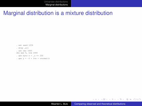
Marginal distribution is a mixture distribution
. set seed 1234
. drop _all
. set obs 1000obs was 0, now 1000
. gen byte x = _n <= 250
. gen y = -3 + 3*x + rnormal()
Maarten L. Buis Comparing observed and theoretical distributions

Univariate distributionsMarginal distributions
Marginal distribution is a mixture distribution. hangroot y, dist(normal) ci name(wrong, replace)(bin=29, start=-6.1794977, width=.30656038)
.
. qui reg y x
. hangroot, ci name(right, replace)(bin=29, start=-6.1794977, width=.30656038)
−5
05
10sq
rt(f
requ
ency
)
−6 −4 −2 0 2y
95% Conf. Int.
−5
05
10sq
rt(f
requ
ency
)
−6 −4 −2 0 2y
95% Conf. Int.
Maarten L. Buis Comparing observed and theoretical distributions
Univariate distributionsMarginal distributions
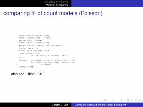
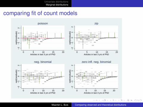
comparing fit of count models (Poisson)
. use "`home´\couart2", clear(Academic Biochemists / S Long)
. gen lnment = ln(ment)(90 missing values generated)
. qui poisson art fem mar kid5 phd lnment
. predict lambda, n(90 missing values generated)
. forvalues i=1/20 {2. qui gen sim`i´ = rpoisson(lambda)3. }
. hangroot , sims(sim*) jitter(5) susp notheor ///> title(poisson) name(poiss, replace) ///> legend(off)(start=0, width=1)
also see: Hilbe 2010
Maarten L. Buis Comparing observed and theoretical distributions

Univariate distributionsMarginal distributions
comparing fit of count models (zero inflated Poisson)
. use "`home´\couart2", clear(Academic Biochemists / S Long)
. gen lnment = ln(ment)(90 missing values generated)
. qui zip art fem mar kid5 phd lnment, inflate(_cons)
. predict lambda, xb(90 missing values generated)
. replace lambda = exp(lambda)(825 real changes made)
. predict pr, pr
. forvalues i=1/20 {2. qui gen sim`i´ = cond(runiform()< pr, 0, rpoisson(lambda))3. }
. hangroot , sims(sim*) jitter(5) susp notheor ///> title(zip) name(zip, replace) ///> legend(off)(start=0, width=1)
Maarten L. Buis Comparing observed and theoretical distributions

Univariate distributionsMarginal distributions
comparing fit of count models (negative binomial)
. use "`home´\couart2", clear(Academic Biochemists / S Long)
. gen lnment = ln(ment)(90 missing values generated)
. qui nbreg art fem mar kid5 phd lnment
. predict xb, xb(90 missing values generated)
. tempname a ia
. scalar `a´ = e(alpha)
. scalar `ia´ = 1/`a´
. gen exb = exp(xb)(90 missing values generated)
. gen xg = .(915 missing values generated)
. gen xbg = .(915 missing values generated)
. forvalues i = 1/20 {2. qui replace xg = rgamma(`ia´, `a´)3. qui replace xbg = exb*xg4. qui generate sim`i´ = rpoisson(xbg)5. }
. hangroot , sims(sim*) jitter(5) susp notheor ///> title(neg. binomial) ///> legend(off) name(nb, replace)(start=0, width=1)
also see: Hilbe 2010
Maarten L. Buis Comparing observed and theoretical distributions
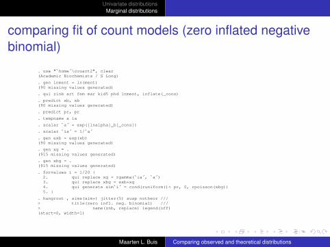
Univariate distributionsMarginal distributions
comparing fit of count models (zero inflated negativebinomial)
. use "`home´\couart2", clear(Academic Biochemists / S Long)
. gen lnment = ln(ment)(90 missing values generated)
. qui zinb art fem mar kid5 phd lnment, inflate(_cons)
. predict xb, xb(90 missing values generated)
. predict pr, pr
. tempname a ia
. scalar `a´ = exp([lnalpha]_b[_cons])
. scalar `ia´ = 1/`a´
. gen exb = exp(xb)(90 missing values generated)
. gen xg = .(915 missing values generated)
. gen xbg = .(915 missing values generated)
. forvalues i = 1/20 {2. qui replace xg = rgamma(`ia´, `a´)3. qui replace xbg = exb*xg4. qui generate sim`i´ = cond(runiform()< pr, 0, rpoisson(xbg))5. }
. hangroot , sims(sim*) jitter(5) susp notheor ///> title(zero infl. neg. binomial) ///> name(znb, replace) legend(off)(start=0, width=1)
Maarten L. Buis Comparing observed and theoretical distributions
Univariate distributionsMarginal distributions
comparing fit of count models−
2−
10
12
sqrt
(res
idua
ls)
0 5 10 15 20Articles in last 3 yrs of PhD
poisson
−2
−1
01
2sq
rt(r
esid
uals
)
0 5 10 15 20Articles in last 3 yrs of PhD
zip
−2
−1
01
2sq
rt(r
esid
uals
)
0 5 10 15 20Articles in last 3 yrs of PhD
neg. binomial
−2
−1
01
2sq
rt(r
esid
uals
)
0 5 10 15 20Articles in last 3 yrs of PhD
zero infl. neg. binomial
Maarten L. Buis Comparing observed and theoretical distributions

Univariate distributionsMarginal distributions
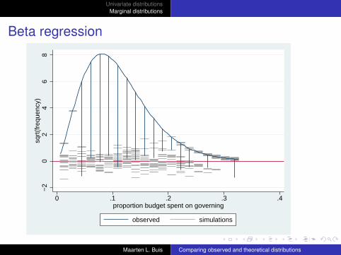
Beta regression
. use "`home´\citybudget", clear(Spending on different categories by Dutch cities in 2005)
. qui betafit governing, mu(noleft minorityleft popdens houseval)
.
. predict a, alpha(1 missing value generated)
. predict b, beta(1 missing value generated)
. forvalues i = 1/20 {2. qui gen sim`i´ = rbeta(a,b)3. }
.
. hangroot, sims(sim*) jitter(5)(bin=20, start=.00440596, width=.01610095)
Maarten L. Buis Comparing observed and theoretical distributions
Univariate distributionsMarginal distributions
Beta regression−
20
24
68
sqrt
(fre
quen
cy)
0 .1 .2 .3 .4proportion budget spent on governing
observed simulations
Maarten L. Buis Comparing observed and theoretical distributions

Univariate distributionsMarginal distributions
Cumulative density function. margdistfit, cumul
0.2
.4.6
.81
Pr(
Y ≤
y)
0 .1 .2 .3 .4proportion budget spent on governing
simulations observedtheoretical
Maarten L. Buis Comparing observed and theoretical distributions

Univariate distributionsMarginal distributions
PP-plot. margdistfit, pp
0.2
.4.6
.81
theo
retic
al P
r(Y
≤ y
)
0 .2 .4 .6 .8 1Empirical Pr(Y ≤ y) = i/(N+1)
simulations observedreference
Maarten L. Buis Comparing observed and theoretical distributions

Univariate distributionsMarginal distributions
QQ-plot. margdistfit, qq
0.1
.2.3
.4pr
opor
tion
budg
et s
pent
on
gove
rnin
g
0 .1 .2 .3 .4theoretical quantiles
simulations observedreference
Maarten L. Buis Comparing observed and theoretical distributions

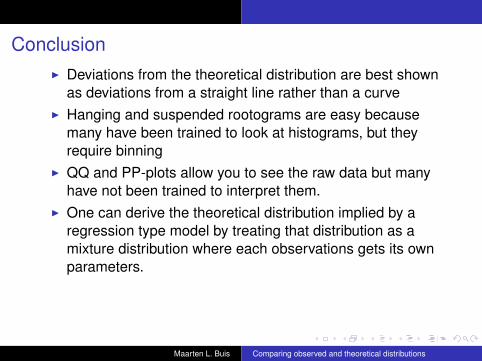
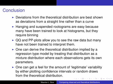
ConclusionI Deviations from the theoretical distribution are best shown
as deviations from a straight line rather than a curve
I Hanging and suspended rootograms are easy becausemany have been trained to look at histograms, but theyrequire binning
I QQ and PP-plots allow you to see the raw data but manyhave not been trained to interpret them.
I One can derive the theoretical distribution implied by aregression type model by treating that distribution as amixture distribution where each observations gets its ownparameters.
I One can get a feel for the amount of ‘legitimate’ variabilityby either plotting confidence intervals or random drawsfrom the theoretical distribution.
Maarten L. Buis Comparing observed and theoretical distributions

ConclusionI Deviations from the theoretical distribution are best shown
as deviations from a straight line rather than a curveI Hanging and suspended rootograms are easy because
many have been trained to look at histograms, but theyrequire binning
I QQ and PP-plots allow you to see the raw data but manyhave not been trained to interpret them.
I One can derive the theoretical distribution implied by aregression type model by treating that distribution as amixture distribution where each observations gets its ownparameters.
I One can get a feel for the amount of ‘legitimate’ variabilityby either plotting confidence intervals or random drawsfrom the theoretical distribution.
Maarten L. Buis Comparing observed and theoretical distributions

References
Goodman, Leo A.On Simultaneous Confidence Intervals for Multinomial Proportions.Technometrics, 7(2):247–254, 1965.
Hilbe, Joseph M.Creating synthetic discrete-response regression modelsThe Stata Journal, 10(1):104–124, 2010.
Tukey, John W.Some Graphic and Semigraphic Displays.in: T.A. Bancroft and S.A. Brown, eds., Statistical Papers in Honor of George W. Snedecor. Ames, Iowa: TheIowa State University Press, pp 293-316, 1972.
Tukey, John W.Exploratory Data Analysis,Addison-Wesley, 1977.
Maarten L. Buis Comparing observed and theoretical distributions