comparison and analysis of datasets van der meer and van
TRANSCRIPT

M.Sc. Thesis
Marcel Mertens
Stability of rock on slopes under wave attack
Comparison and analysis of datasets
VAN DER MEER [1988] and VAN GENT ET AL. [2003]

Delft University of Technology
Faculty of Civil Engineering
Department of Hydraulic Engineering
M.Sc. Thesis
April 2007
Graduation Committee: Graduation Student:
Prof. Dr. Ir. M.J.F. Stive Ing. M. Mertens
Ir. H.J. Verhagen
Dr. Ir. J.W. Van der Meer
Drs. R. Booij
Stability of rock on slopes under wave attack
Comparison and analysis of datasets
VAN DER MEER [1988] and VAN GENT ET AL. [2003]

I
PREFACE
This document contains the final report of my M.Sc. Thesis at Delft University of
Technology, faculty of Civil Engineering, department of Hydraulic Engineering. This report
can be used as a starting point to further research on this topic. During the work on this
M.Sc. Thesis and because of the great amount of data sometimes it was really difficult not to
make the same mistakes which formed the basis of this report. Also for me it became clear
how difficult it is to prove empirical relations in processes that are not yet fully understood.
This M.Sc. Thesis is another step closer to a clear solution on this topic.
This M.Sc. Thesis would not have succeeded without the great help and patience of Mr.
Verhagen who really was of great support for me. Also I would like to thank the other
members of the graduation committee Mr. Stive, Mr. Van der Meer and Mr. Booij for their
support and guidance and Mr. Van Gent for providing his graphs. Last but not least I would
like to thank my parents and my girlfriend for their great support and patience during my
whole study.
Marcel Mertens
Delft, April 2007

II
ABSTRACT
On the stability of rock in the twentieth century a lot of research has been done. In VAN DER
MEER [1988] two stability formulae were presented for breakwater design that were later
generally accepted in the engineering practice. Most of the tests of VAN DER MEER [1988]
were done with foreshore deep water conditions. In practice however structures with
shallow foreshores showed more damage than average. This was a starting point for the
work of VAN GENT ET AL. [2003], who did most of the tests with shallow water conditions.
In VAN GENT [2004] graphs were presented in which the datasets of VAN DER MEER [1988]
and VAN GENT ET AL. [2003] were compared. These graphs are presented in Figure 0.1.
Figure 0.1: Data VAN GENT ET AL. [2003] (blue) compared with data VAN DER MEER [1988] (red) for plunging (left) and surging waves (right)

ABSTRACT III
There has been a lot of discussion about the graphs as presented in Figure 0.1. It can be seen
that differences occur between the two datasets. However one problem was that the two
datasets were not compared in a proper way because a number of parameters were not
correctly transformed in a comparable format. Therefore in this M.Sc. Thesis the datasets
were analysed and all parameters were individually transformed in a proper way so that a
good comparison can be made. After that possible explanations for the differences were
discussed.
For the dataset of VAN DER MEER [1988] differences occurred between the original graphs for
plunging and surging waves and the reconstructed graphs which could not be explained by
errors in the spreadsheet. After a thorough investigation of these differences it could be seen
that mistakes were made in the original graphs of VAN DER MEER [1988]. Some points which
did not appear in the graph for plunging waves appeared in the graph for surging waves
and vice versa. A probable reason for this is that mistakes were made with the use of the
boundary between plunging and surging waves. In the development of the formulae of VAN
DER MEER [1988] different values of P were used in order to describe the permeability of the
structures. In this way the boundary between plunging and surging waves, which depends
on the permeability, also varied during experiments, which probably caused the mistakes.
Also it must be mentioned that at the time the PhD thesis was written less sophisticated
computer programmes were used.
The dataset of VAN GENT ET AL. [2003] was not available for this M.Sc. Thesis. Data could
only be read of from the graphs presented in VAN GENT ET AL. [2003]. To be able to make a
good comparison the data coordinates from the original graphs were entered in the
spreadsheet. Because of the unavailability of the data of VAN GENT ET AL. [2003] no changes
to this dataset can be made. The dataset of THOMPSON & SHUTTLER [1975] which was a
starting point for the work of VAN DER MEER [1988] was also entered in the spreadsheet.
After this in the digitalised datasets parameters had to be transformed. In the dataset of
THOMPSON & SHUTTLER [1975] the damage level was indicated with the parameter N∆, which
had to be transformed to the damage parameter S, that was used by VAN DER MEER [1988]
and VAN GENT ET AL. [2003]. Also for the stone diameter THOMPSON & SHUTTLER [1975] used
a different parameter. In VAN DER MEER [1988] and THOMPSON & SHUTTLER [1975] for the
wave height the significant wave height, Hs, has been used, while in VAN GENT ET AL. [2003]
the wave height exceeded by 2% of the waves, H2%, was used.

ABSTRACT IV
Using the approach of BATTJES & GROENENDIJK [2000] the wave height was transformed for
each point individually. For the wave period VAN DER MEER [1988] and THOMPSON &
SHUTTLER [1975] used the mean period, Tm. VAN GENT ET AL. [2003] however showed that it
is better to use the spectral period, Tm-1,0, for stability calculations. The transformation from
the mean period, Tm, to the spectral period, Tm-1,0, depends on the spectral shape. For the
dataset of VAN DER MEER [1988] the spectra that were used were indicated as PM (Pierson
Moskowitz) spectra, narrow- and wide spectra. A close inspection of these spectra showed
that all these spectra are quite a lot narrower than they should be. Therefore for each
spectrum that was used the transformation to the spectral wave period was done for each
point individually using the correct spectrum.
In VAN DER MEER [1988] it was already mentioned that data with different spectra showed
more damage than average especially for surging waves. These differences could not be
caused by the difference in spectra, but a possible explanation was the effect of rounding due
to frequent handling and the painting process. LATHAM ET AL. [1988] did some research to
the effects of roundness on stability with stones of different roundness, where also
subsamples from the stones used by VAN DER MEER [1988] were tested. In LATHAM ET AL.
[1988] correction factors for the stability formulae were presented to include the effects of
roundness Including these factors in the formulae for the dataset of VAN DER MEER [1988]
gives remarkable effects, which are visualized in Figure 0.2.
Figure 0.2: The effects of including the roundness parameter, γLatham, on the graphs of the dataset for surging waves of VAN DER MEER [1988]
0,0
0,5
1,0
1,5
2,0
0,0 0,2 0,4 0,6 0,8 1,0 1,2 1,4 1,6
Surging waves (original graph)
Surging waves (with influence roundness)
H2%/∆Dn50 · ξm-1,0-P · P0,13 · tanα0,5 [-]
S/N
0,5 [-
]
S/N
0,5 [-
]
γLatham;su·H2%/∆Dn50 · ξm-1,0-P · P0,13 · tanα0,5 [-]
0,0
0,5
1,0
1,5
2,0
0,0 0,2 0,4 0,6 0,8 1,0 1,2 1,4 1,6
ABSTRACT V
0,0
0,5
1,0
1,5
2,0
0,0 0,2 0,4 0,6 0,8 1,0 1,2 1,4 1,60,0
0,5
1,0
1,5
2,0
0 1 2 3 4 5 6 7 8 9 10
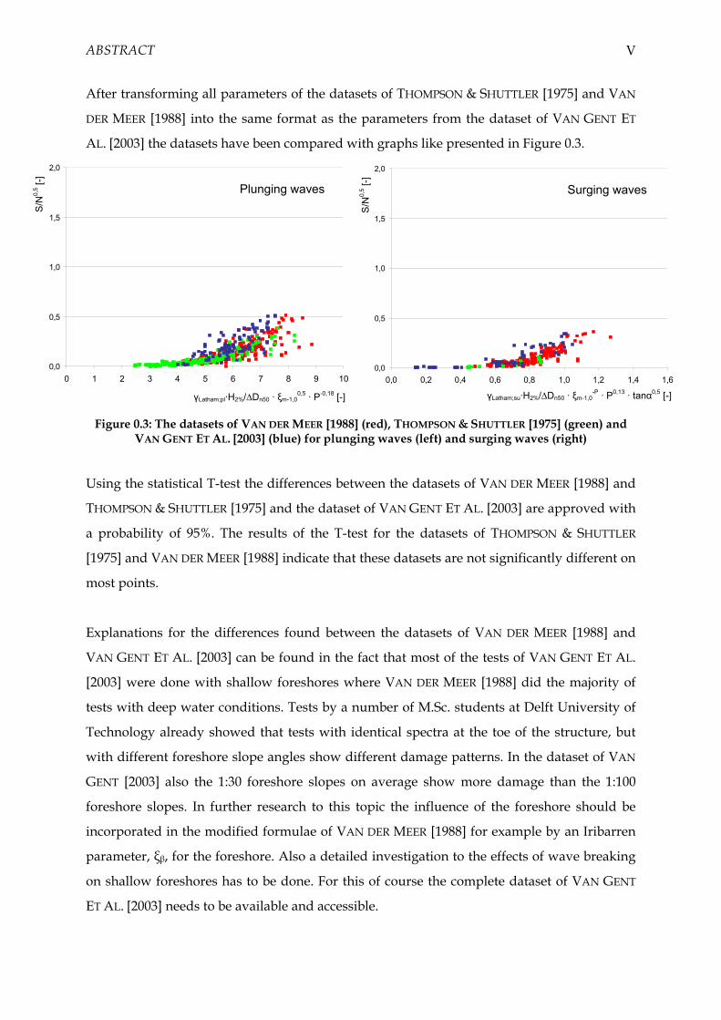
After transforming all parameters of the datasets of THOMPSON & SHUTTLER [1975] and VAN
DER MEER [1988] into the same format as the parameters from the dataset of VAN GENT ET
AL. [2003] the datasets have been compared with graphs like presented in Figure 0.3.
Figure 0.3: The datasets of VAN DER MEER [1988] (red), THOMPSON & SHUTTLER [1975] (green) and VAN GENT ET AL. [2003] (blue) for plunging waves (left) and surging waves (right)
Using the statistical T-test the differences between the datasets of VAN DER MEER [1988] and
THOMPSON & SHUTTLER [1975] and the dataset of VAN GENT ET AL. [2003] are approved with
a probability of 95%. The results of the T-test for the datasets of THOMPSON & SHUTTLER
[1975] and VAN DER MEER [1988] indicate that these datasets are not significantly different on
most points.
Explanations for the differences found between the datasets of VAN DER MEER [1988] and
VAN GENT ET AL. [2003] can be found in the fact that most of the tests of VAN GENT ET AL.
[2003] were done with shallow foreshores where VAN DER MEER [1988] did the majority of
tests with deep water conditions. Tests by a number of M.Sc. students at Delft University of
Technology already showed that tests with identical spectra at the toe of the structure, but
with different foreshore slope angles show different damage patterns. In the dataset of VAN
GENT [2003] also the 1:30 foreshore slopes on average show more damage than the 1:100
foreshore slopes. In further research to this topic the influence of the foreshore should be
incorporated in the modified formulae of VAN DER MEER [1988] for example by an Iribarren
parameter, ξβ, for the foreshore. Also a detailed investigation to the effects of wave breaking
on shallow foreshores has to be done. For this of course the complete dataset of VAN GENT
ET AL. [2003] needs to be available and accessible.
Surging waves Plunging waves S
/N0,
5 [-]
γLatham;su·H2%/∆Dn50 · ξm-1,0-P · P0,13 · tanα0,5 [-]
S/N
0,5 [-
]
γLatham;pl·H2%/∆Dn50 · ξm-1,00,5 · P-0,18 [-]

VI
CONTENTS
PREFACE ............................................................................................................................................I
ABSTRACT ......................................................................................................................................... II
CONTENTS........................................................................................................................................VI
LIST OF FIGURES ..............................................................................................................................X
LIST OF TABLES............................................................................................................................ XIV
NOTATIONS .................................................................................................................................. XVI
CHAPTER 1 INTRODUCTION ................................................................................................ 1
1.1 Background....................................................................................................................... 1
1.1.1 Breakwaters and sea defences.......................................................................... 1
1.1.2 Stability of rock .................................................................................................. 2
1.1.3 Iribarren/Hudson.............................................................................................. 3
1.1.4 THOMPSON & SHUTTLER [1975] ........................................................................ 4
1.1.5 VAN DER MEER [1988] ........................................................................................ 5
1.1.6 VAN GENT Et Al. [2003]..................................................................................... 7
1.2 Problem description ........................................................................................................ 9
1.3 Problem definition ......................................................................................................... 10
1.4 Report outline................................................................................................................. 11

CONTENTS VII
CHAPTER 2 VAN DER MEER ................................................................................................ 12
2.1 Introduction .................................................................................................................... 12
2.2 Graph for plunging waves............................................................................................ 12
2.3 Graph for surging waves .............................................................................................. 15
2.4 Explanation differences................................................................................................. 16
2.5 Test results with different spectra ............................................................................... 18
2.6 Conversion dataset to Tm-1,0 and H2% values............................................................... 22
2.6.1 Wave height...................................................................................................... 22
2.6.2 Wave period ..................................................................................................... 25
2.7 Graphs with H2% and Tm-1,0 ........................................................................................... 26
2.8 Influence of stone roundness ....................................................................................... 28
2.9 New graphs of VAN DER MEER [1988] ......................................................................... 37
CHAPTER 3 THOMPSON & SHUTTLER............................................................................ 39
3.1 Introduction .................................................................................................................... 39
3.2 Damage level .................................................................................................................. 39
3.3 Correctness spreadsheet ............................................................................................... 40
3.4 Conversion dataset to Tm-1,0 and H2% values............................................................... 42
3.4.1 Wave height...................................................................................................... 42
3.4.2 Wave period ..................................................................................................... 43
3.5 New graphs of dataset THOMPSON & SHUTTLER [1975] ............................................ 43
CHAPTER 4 VAN GENT.......................................................................................................... 45
4.1 Introduction .................................................................................................................... 45
4.2 Correctness spreadsheet ............................................................................................... 45
CHAPTER 5 COMPARISON OF DATASETS ..................................................................... 47
5.1 Plunging waves.............................................................................................................. 47
5.2 Surging waves ................................................................................................................ 49
5.3 Maximum accepted damage levels ............................................................................. 52
5.4 Detailed graphs for plunging waves........................................................................... 55
5.5 Detailed graphs for surging waves ............................................................................. 56

CONTENTS VIII
CHAPTER 6 STATISTICS........................................................................................................ 58
6.1 Introduction .................................................................................................................... 58
6.2 Basic statistics for plunging waves.............................................................................. 58
6.3 Basic statistics for surging waves ................................................................................ 61
6.4 The T-test......................................................................................................................... 63
6.4.1 VAN GENT ET AL. [2003] – VAN DER MEER [1988]........................................ 63
6.4.2 THOMPSON & SHUTTLER [1975] - VAN DER MEER [1988] ............................. 64
6.4.3 THOMPSON & SHUTTLER [1975] - VAN GENT ET AL. [2003]......................... 65
CHAPTER 7 DESIGN PRACTICE.......................................................................................... 66
7.1 Introduction .................................................................................................................... 66
7.2 Basic statistics for plunging waves.............................................................................. 69
7.3 Basic statistics for surging waves ................................................................................ 72
7.4 The T-test......................................................................................................................... 74
7.4.1 VAN GENT ET AL. [2003] – VAN DER MEER [1988]........................................ 74
7.4.2 THOMPSON & SHUTTLER [1975] - VAN DER MEER [1988] ............................. 75
7.4.3 THOMPSON & SHUTTLER [1975] - VAN GENT ET AL. [2003]......................... 76
CHAPTER 8 ELABORATION DIFFERENCES .................................................................... 77
8.1 Introduction .................................................................................................................... 77
8.2 Influence of shallow foreshores ................................................................................... 77
8.3 Influence of double peaked spectra............................................................................. 86
8.4 Wave breaking................................................................................................................ 88
8.5 Surf beat and wave reflection....................................................................................... 89
CHAPTER 9 CONCLUSIONS AND RECOMMENDATIONS ........................................ 91
9.1 General conclusion ........................................................................................................ 91
9.2 Recommendations ......................................................................................................... 92
REFERENCES .................................................................................................................................... 93

CONTENTS IX
APPENDIX A THEORY............................................................................................................... 95
A1 Wave height distribution on shallow foreshores ...................................................... 95
A2 Wave spectra................................................................................................................... 99
A3 Ratio peak period to spectral period......................................................................... 102
A4 The T-Test...................................................................................................................... 106
APPENDIX B SPECTRA VAN DER MEER [1988]............................................................... 109
APPENDIX C STONES VAN DER MEER [1988]................................................................. 112
APPENDIX D LEGEND GRAPHS VAN DER MEER ......................................................... 117
APPENDIX E DETAILED GRAPHS ...................................................................................... 118

X
LIST OF FIGURES
Figure 0.1: Data VAN GENT ET AL. [2003] (blue) compared with data VAN DER MEER [1988] (red) for plunging (left) and surging waves (right)..................................................II
Figure 0.2: The effects of including the roundness parameter, γLatham, on the graphs of the dataset for surging waves of VAN DER MEER [1988]............................................... IV
Figure 0.3: The datasets of VAN DER MEER [1988] (red), THOMPSON & SHUTTLER [1975] (green) and VAN GENT ET AL. [2003] (blue) for plunging waves (left) and surging waves (right)...............................................................................................................................V
Figure 1.1: Plunging breaker (left) and surging breaker (right)......................................................2
Figure 1.2: Model set up of VAN DER MEER [1988]............................................................................5 Figure 1.3: Model set up VAN GENT ET AL. [2003]............................................................................7
Figure 1.4: Data of VAN GENT ET AL. [2003] and VAN DER MEER [1988] .......................................9
Figure 2.1: Plunging waves (VAN DER MEER [1988]) ......................................................................13 Figure 2.2: Plunging waves VAN DER MEER [1988] (permeable, impermeable, homogenous).14 Figure 2.3: Surging waves (VAN DER MEER [1988]).........................................................................15 Figure 2.4: Surging waves VAN DER MEER [1988] (only permeable, impermeable and
homogenous) ................................................................................................................16 Figure 2.5: Plunging waves VAN DER MEER [1988] (only different spectra)................................18 Figure 2.6: Surging waves VAN DER MEER [1988] (only different spectra) ..................................19
Figure 2.7: Spectra used in VAN DER MEER [1988] ..........................................................................21

LIST OF FIGURES XI
Figure 2.8: Calculated m0 compared with exact m0 (left : GODA [1988] ; right : average ratios)24 Figure 2.9: Differences due calculated or measured value of Tp ..................................................25 Figure 2.10: Plunging waves with H2% and Tm-1,0 from dataset VAN DER MEER [1988] ..............27 Figure 2.11: Surging waves with H2% and Tm-1,0 from dataset VAN DER MEER [1988]................27 Figure 2.12: Riprap after 134 tests, 2x painted.................................................................................28 Figure 2.13: Uniform stone after 106 tests, 1x painted ...................................................................29 Figure 2.14: Uniform stone after 41 tests, not painted....................................................................29 Figure 2.15: Quarry run after 10 tests, not painted.........................................................................29 Figure 2.16: Basalt after 10 tests, not painted...................................................................................29 Figure 2.17: Tabular stones, LATHAM ET AL. [1988] ........................................................................31 Figure 2.18: Equant stones, LATHAM ET AL. [1988]..........................................................................31
Figure 2.19: Fresh stones, LATHAM ET AL. [1988].............................................................................32 Figure 2.20: Semi round stones, LATHAM ET AL. [1988]..................................................................32 Figure 2.21: Very round stones, LATHAM ET AL.1988] ....................................................................32 Figure 2.22: Pr - cpl and Pr - csu plots from LATHAM ET AL. [1988]: Left P=0,05; right P=0,1 .....34 Figure 2.23: Effects of influence stone-roundness on graphs of VAN DER MEER [1988] ............36 Figure 2.24: New graph for Plunging waves of VAN DER MEER [1988] .......................................37
Figure 2.25: New graph for surging waves of VAN DER MEER [1988] ..........................................38
Figure 3.1: THOMPSON & SHUTTLER [1975] and VAN DER MEER [1988] for plunging waves.....40 Figure 3.2: THOMPSON & SHUTTLER [1975] and VAN DER MEER [1988] for surging waves .......41 Figure 3.3: Plunging waves THOMPSON & SHUTTLER [1975] .........................................................43 Figure 3.4: Surging waves THOMPSON & SHUTTLER [1975]............................................................44
Figure 4.1: Plunging waves, reconstructed graph (grey), original graph (VAN GENT ET AL. [2003]).............................................................................................................................46
Figure 4.2: Surging waves, reconstructed graph (grey), original graph VAN GENT ET AL. [2003] ..............................................................................................................................46
Figure 5.1: Plunging waves: THOMPSON & SHUTTLER [1975] (green), VAN DER MEER [1988] (red), VAN GENT ET AL. [2003] (blue..........................................................................47
Figure 5.2: Plunging waves: VAN DER MEER [1988] (red), VAN GENT ET AL. [2003] (blue).......48 Figure 5.3: Plunging waves: THOMPSON & SHUTTLER [1975] (green), VAN GENT ET AL. [2003]
(blue) ..............................................................................................................................48 Figure 5.4: Plunging waves: THOMPSON & SHUTTLER [1975] (green), VAN DER MEER [1988]
(red) ................................................................................................................................49

LIST OF FIGURES XII
Figure 5.5: Surging waves: THOMPSON & SHUTTLER [1975] (green), VAN DER MEER [1988] (red), VAN GENT ET AL. [2003] (blue).........................................................................50
Figure 5.6: Surging waves: VAN DER MEER [1988] (red), VAN GENT ET AL. [2003] (blue) .........50 Figure 5.7: Surging waves: THOMPSON & SHUTTLER [1975] (green), VAN GENT ET AL. [2003]
(blue) ..............................................................................................................................51 Figure 5.8: Surging waves: THOMPSON & SHUTTLER [1975] (green), VAN DER MEER [1988] (red)51 Figure 5.9: Plunging waves: THOMPSON & SHUTTLER [1975] (green), VAN DER MEER [1988]
(red), VAN GENT ET AL. [2003] (blue) with maximal acceptable damage levels .53 Figure 5.10: Surging waves: THOMPSON & SHUTTLER [1975] (green), VAN DER MEER [1988]
(red), VAN GENT ET AL. [2003] (blue) with maximal acceptable damage levels .54 Figure 5.11: Plunging waves: THOMPSON & SHUTTLER [1975] (green), VAN DER MEER [1988]
(red), VAN GENT ET AL. [2003] (blue) with maximal acceptable damage levels .55 Figure 5.12: Plunging waves: 5% and 95% Exceedance lines, THOMPSON & SHUTTLER [1975]
(green), VAN DER MEER [1988] (red), VAN GENT ET AL. [2003] (blue) ...................55 Figure 5.13: Surging waves: THOMPSON & SHUTTLER [1975] (green), VAN DER MEER [1988]
(red), VAN GENT ET AL. [2003] (blue) with maximal acceptable damage levels .56 Figure 5.14: Surging waves: 5% and 95% Exceedance lines, THOMPSON & SHUTTLER [1975]
(green), VAN DER MEER [1988] (red), VAN GENT ET AL. [2003] (blue) ...................57
Figure 6.1: Mean values (step size 0,5) for plunging waves..........................................................60 Figure 6.2: Standard deviation (step size 0,5) for plunging waves ..............................................60 Figure 6.3: Mean values (step size 0,1) for surging waves.............................................................62
Figure 6.4: Standard deviation (step size 0,1) for surging waves .................................................62
Figure 7.1: Plunging waves with switched axes, VAN DER MEER [1988] (red), THOMPSON & SHUTTLER [1975] (green), VAN GENT ET AL. [2003] (blue) .....................................67
Figure 7.2: Surging waves with switched axes, VAN DER MEER [1988] (red), THOMPSON & SHUTTLER [1975] (green), VAN GENT ET AL. [2003] (blue) .....................................67
Figure 7.3: 5% and 95% exceedance lines for plunging waves with switched axes, VAN DER MEER [1988] (red), THOMPSON & SHUTTLER [1975] (green), VAN GENT ET AL. [2003] (blue)...................................................................................................................68
Figure 7.4: 5% and 95% exceedance lines for surging waves with switched axes, VAN DER MEER [1988] (red), THOMPSON & SHUTTLER [1975] (green), VAN GENT ET AL. [2003] (blue)...................................................................................................................69
Figure 7.5: Mean values (step size = 0,04) for plunging waves with switched axes..................71 Figure 7.6: Standard deviation (step size = 0,04) for plunging waves with switched axes ......71 Figure 7.7: Mean values (step size = 0,04) for surging waves with switched axes ....................73
Figure 7.8: Standard deviation (step size = 0,04) for surging waves with switched axes .........73

LIST OF FIGURES XIII
Figure 8.1: Decrease of phase shift between velocity (red) and acceleration (blue) ..................78 Figure 8.2: Plunging waves: VAN DER MEER [1988] and THOMPSON & SHUTTLER [1975] (grey),
VAN DER MEER [1988] with shallow foreshores (red), VAN GENT ET AL. [2003] (blue) ..............................................................................................................................79
Figure 8.3: Surging waves: VAN DER MEER [1988] and THOMPSON & SHUTTLER [1975] (grey), VAN DER MEER [1988] with shallow foreshores (red), VAN GENT ET AL. [2003] (blue) ..............................................................................................................................80
Figure 8.4: Plunging waves: VAN GENT ET Al. [2003] cotβ=30 (dark blue), cotβ=100 (light blue), VAN DER MEER [1988] with cotβ=30 (red) ....................................................81
Figure 8.5: Surging waves: VAN GENT ET Al. [2003] cotβ=30 (dark blue), cotβ=100 (light blue), VAN DER MEER [1988] with cotβ=30 (red) ..................................................81
Figure 8.6: Model setup with deep water at toe and foreshore slope cotβ=∞ ...........................83 Figure 8.7: Model setup with shallow water at toe and foreshore slope cotβ=∞ .......................83 Figure 8.8: Model setup with shallow water at toe and foreshore slope cotβ=100....................84 Figure 8.9: Model setup with shallow water at toe and foreshore slope cotβ=30......................84
Figure 8.10: Plunging waves: VAN GENT ET AL. [2003] Single peaked spectra, double peaked spectra ............................................................................................................................87
Figure 8.11: Surging waves: VAN GENT ET AL. [2003] Single peaked spectra), double peaked spectra ............................................................................................................................87
Figure 8.12: Plunging waves VAN GENT ET AL. [2003] with distinction in amount of wave breaking .........................................................................................................................88
Figure 8.13: Plunging waves (left) and surging waves (right) of VAN DER MEER [1988] and THOMPSON & SHUTTLER with distinction in Hs<0,10m (blue) and Hs>0,10m (red)90
Figure A.1: Probability density function (BATTJES & GROENENDIJK [2000]) ................................95 Figure A.2: PM- spectrum and JONSWAP-spectrum ..................................................................101 Figure A.3: Wave spectrum with cut-of frequency and 40%- and 80% energy value .............103
Figure A.4: Idealized distributions for treated and comparison group posttest values .........106 Figure A.5: Three scenarios for differences between means .......................................................107
FigureA.6: Plunging waves with maximum accepted damage levels: THOMPSON & SHUTTLER [1975] (green), VAN DER MEER [1988] (red), VAN GENT ET AL. [2003] (blue) .....118
FigureA.7: Surging waves with maximum accepted damage levels: THOMPSON & SHUTTLER [1975] (green), VAN DER MEER [1988] (red), VAN GENT ET AL. [2003] (blue) .....119

XIV
LIST OF TABLES
Table 2.1: Deviating points in graphs for plunging and surging waves .....................................17
Table 2.2: Values of m0 for the 15 tests of DELFT HYDRAULICS, M1983 PART I ............................23 Table 2.3: Average values of Hs/√m0 for 3 different spectra.........................................................24 Table 2.4: Ratios peak period / spectral period and corresponding standard deviations........26 Table 2.5: Stone types used in VAN DER MEER [1988] .....................................................................28
Table 2.6: Shape and roughness factors for stones from LATHAM ET AL. [1988].........................31 Table 2.7: Shape and roughness factors for subsamples from VAN DER MEER [1988] ...............32 Table 2.8: Influence stone roundness on coefficients Van der Meer formulae ...........................35
Table 3.1: Conversion from NΔ to S...................................................................................................40
Table 5.1: Damage levels THOMPSON & SHUTTLER [1975] and VAN DER MEER [1988] ...............52
Table 5.2: Damage levels VAN GENT ET AL. [2003].........................................................................53
Table 6.1: Basic statistical values for plunging waves....................................................................59 Table 6.2: Basic statistical values for surging waves ......................................................................61
Table 6.3: The T-test for VAN GENT ET AL. [2003] and VAN DER MEER [1988] for plunging waves..............................................................................................................................63
Table 6.4: The T-test for VAN GENT ET AL. [2003] and VAN DER MEER [1988] for surging waves..............................................................................................................................64
Table 6.5: The T-test for THOMPSON & SHUTTLER [1975] and VAN DER MEER [1988] .................64

LIST OF TABLES XV
Table 6.6: The T-test for THOMPSON & SHUTTLER [1975] and VAN DER MEER [1988] for surging waves..............................................................................................................................64
Table 6.7: The T-test for THOMPSON & SHUTTLER [1975] and VAN GENT ET AL. [2003].............65 Table 6.8: The T-test for THOMPSON & SHUTTLER [1975] and VAN GENT ET AL. [2003] for
surging waves ...............................................................................................................65
Table 7.1: Basic statistical values for plunging waves with switched axes .................................70 Table 7.2: Basic statistical values for surging waves ......................................................................72 Table 7.3: The T-test for VAN GENT ET AL. [2003] and VAN DER MEER [1988] for plunging
waves..............................................................................................................................74 Table 7.4: The T-test for VAN GENT ET AL. [2003] and VAN DER MEER [1988] for surging
waves..............................................................................................................................74 Table 7.5: The T-test for THOMPSON & SHUTTLER [1975] and VAN DER MEER [1988] .................75 Table 7.6: The T-test for THOMPSON & SHUTTLER [1975] and VAN DER MEER [1988] for surging
waves..............................................................................................................................75
Table 7.7: The T-test for THOMPSON & SHUTTLER [1975] and VAN GENT ET AL. [2003].............76 Table 7.8: The T-test for THOMPSON & SHUTTLER [1975] and VAN GENT ET AL. [2003] for
surging waves ...............................................................................................................76
Table 8.1: Behaviour of foreshore Iribarren parameter for tests of VAN DER MEER [1988]........85
Table A.1: table from Battjes & Groenendijk [2000] for H2% and H1/3..........................................98
Table A.2: Ratios Tp / Tm-1,0 for tests from DELFT HYDRAULICS, M1983 PART I [1988] ............104 Table A.3: Average ratios peak period / spectral period and standard deviations ................105

XVI
NOTATIONS
a = Amplitude [m]
Ai = erosion area in a cross-section (indices 1, 2, 3) [m2]
A1 = accretion area in beach crest area [m2]
A2 = erosion area [m2]
A3 = accretion area below the water surface [m2]
An = phase angle in Fourier series [-]
cplunging, cpl = regression coefficient in formula of VAN DER MEER [1988] for
plunging waves
[-]
cplunging, csu = regression coefficient in formula of VAN DER MEER [1988] for
plunging waves
[-]
Cn = amplitude coefficient of the nth harmonic in Fourier series [-]
d = water depth [m]
dforeshore = water depth on foreshore [m]
dof = degrees of freedom in T-test [-]
D = Duration of a wave record [s]
D = Diameter [m]
D15 = Sieve diameter exceeded by 15% of the stones [m]
D50 = Sieve diameter exceeded by 50% of the stones [m]
D85 = Sieve diameter exceeded by 85% of the stones [m]

NOTATIONS XVII
Dn = nominal diameter (W/ρa)1/3 [m]
Dn50 = nominal diameter exceeded by 50% of the stones [m]
f = Frequency [Hz]
g = gravitational acceleration [m/s2]
H = Wave height [m]
H1, H2 = Scale parameters in Composite Weibull distribution [-]
Hs = (incoming) significant wave height [m]
H2% = Wave height exceeded by 2% of the waves [m]
H1/3 = average of the highest 1/3 of the wave heights in a wave record [m]
Hm0 = 4 times the standard deviation of the surface elevation [m]
Hrms = root mean square wave height [m]
Htr = transitional wave height in Composite Weibull distribution [m]
k1,k2 = shape parameters of the distribution determining the curvature in
Composite Weibull distribution
[-]
L = Wave length [m]
L0 = Deep water wave length (=gT2/2π) [m]
m0 = zero-th order spectral moment [-]
m-1 = first order negative spectral moment [-]
n = number of tests [-]
NIribarren = dustbin factor in stability formula of IRIBARREN [1938] [-]
NΔ = damage parameter defined in THOMPSON & SHUTTLER [1975] [-]
N = number of waves [-]
P = permeability coefficient defined in VAN DER MEER [1988] [-]
Pf = fictitious porosity =100(1-(ρa/ρb)) [%]
Pn = Fourier noncircularity, based on harmonic amplitudes from 1 to ∞ [-]
PC = Fourier shape contribution factor (=10Pn) (LATHAM ET AL. [1988]) [-]
PR = Fourier asperity roughness based on the 11th to 20th harmonic
amplitudes as defined in LATHAM ET AL. [1988]
[-]
PS = Fourier shape factor based on the 1th to 10th harmonic amplitudes as
defined in LATHAM ET AL. [1988]
[-]
PM = Pierson Moskowitz
sd = standard deviation
S = damage level as defined in VAN DER MEER [1988] (=Ai/Dn502) [-]
t = Time [s]

NOTATIONS XVIII
tarmour = thickness armour layer [m]
tfilter = thickness filter layer [m]
tobs = ratio between difference and variability of two groups (T-test) [-]
T = Wave period [s]
Tm = Mean wave period [s]
Tm-1,0 = spectral wave period m-1/m0 [s]
Tm-1,0;a spectral wave period Tm-1,0 using a cut-off frequency for the lower
frequencies
[s]
Tp = Peak wave period [s]
Tp;a the peak period using a cut off frequency for the higher frequencies. [s]
Tp;b The peak period Tm-1,0 from the part of the spectrum for which the
energy is more than 40% of the maximum value
[s]
Tp;d The peak period Tm-1,0 from the part of the spectrum for which the
energy is more than 80% of the maximum value
[s]
W = weight of stone/block [N]
X = group mean of group X (x1, x2, ……..xn)
Y = group mean of group Y (y1, y2, ……..yn)
α = Slope angle of construction [-]
β = Slope angle of foreshore [-]
βtr = Slope-dependent coefficient in calculation of Htr [-]
γLatham = correction factor for the influence of stone roundness according to
LATHAM ET AL. [1988])
[-]
Δ = relative density: (ρr – ρw)/ ρw [-]
η(t) = the surface elevation in a time record reproduced as the sum of a
large number of harmonic wave components (Fourier series)
[m]
θ = Polar angle measured from an arbitrary reference line [-]
μ = friction coefficient [-]
ξβ = Iribarren parameter for the foreshore ξβ=tanβ/√(H/L) [-]
ξc = Critical Iribarren parameter indicating transition between plunging
and surging waves
[-]
ξm = Iribarren parameter calculated with Tm [-]
ξm-1,0 = Iribarren parameter calculated with Tm-1,0 [-]

NOTATIONS XIX
ξp = Iribarren parameter calculated with Tp [-]
ρa = Mass density of stone [kg/m3]
ρb = bulk density of material as laid on the slope [kg/m3]
ρw = density of water [kg/m3]
ρr = density of stone/block (rock) [kg/m3]

1
Chapter 1 INTRODUCTION
INTRODUCTION
1.1 Background
A lot of research has been done to the stability of stones or sediments. In this we can
distinguish stability due currents, waves or a combination of the two. This M.Sc. Thesis deals
with the stability of rock on a slope, attacked by waves. Practical applications of rock on a
slope are breakwaters and sea– or inland water defences.
1.1.1 Breakwaters and sea defences
Breakwaters are generally shore-parallel structures that reduce the amount of wave energy
(wave height) reaching the protected area. They are similar to natural bars, reefs or near
shore islands and are designed to dissipate wave energy. In high wave energy environments
breakwaters are usually constructed using large armour stone, or pre-cast concrete units or
blocks. Where stone weight and interlocking are important stability mechanisms. In lower
wave-energy environments, grout-filled fabric bags, gabions and other proprietary units are
common used. Typical rubble mound breakwater design is similar to that of a revetment,
with a core or filter layer of smaller stone, overlain by the armouring layer of armour stone
or pre-cast concrete units. Special types of breakwaters are caisson breakwaters and floating
breakwaters, which will not be discussed in this M.Sc. Thesis.

INTRODUCTION 2
1.1.2 Stability of rock
Movement of stones and sediments due to currents or waves does only occur when the
acting forces out of the water motion, like drag and lift forces, exceed friction and weight
forces. Whether a particle is moving or not is described in so-called threshold conditions.
Because of the complex water movement of waves breaking on a slope fully theoretical
expressions for the forces and the stability of the stones are very hard to derive. Therefore a
number of empirical formulae have been developed, all based on results of small-scale
experiments. In these formulae stability of an individual stone is often defined by a ratio of
the unit size (weight/length scale) and the wave height. Movement of stones does not
automatically mean failure. As long as the armour layer is able to protect the underlying
filter layer (existing out of smaller stones which will easily be moved) the structure has not
failed. Depending on the amount of damage a construction needs to be repaired after a
severe storm.
In stability formulae sometimes a distinction is made between plunging and surging waves.
The difference between these two types of wave breaking is shown in Figure 1.1.
Figure 1.1: Plunging breaker (left) and surging breaker (right)
Plunging breakers overall are the result of steeper waves over moderate slopes, where wave
energy is released suddenly as the crest curls and then descends violently. This is a typical
“surfer” wave, it breaks very quickly and with substantial force. Surging breakers mostly
occur when the beach slope exceeds wave steepness and are usually found on very steep
slopes. The wave does not really curl and break in the traditional way but runs up against
the shore while producing foam and large surges of water. A surging wave often starts as a
plunging wave, then the wave catches up with the crest, and the breaker surges up slope as a
wall of water, with the wave crest and base travelling at the same speed. This results in a
quickly rising and falling water level on the shore face.

INTRODUCTION 3
1.1.3 Iribarren/Hudson
For many years breakwater design was a question of trial and error. In 1938 in IRIBARREN
[1938] a theoretical model for the stability of stone on a slope under wave attack was
developed. IRIBARREN [1938] concentrated on a theoretical approach, assisted by some
experiments.
According to IRIBARREN [1938] the forces acting on a stone placed at an angle α are:
• Weight of the stone (acting in vertical downward direction)
• Buoyancy of the stone (acting in vertical upward direction)
• Wave force (acting parallel to the slope, upwards or downwards)
• Frictional resistance (acting parallel to the slope, upwards or downwards, opposite
direction to the wave force)
The design formula of IRIBARREN [1938] distinguishes downrush and uprush along the slope.
According to IRIBARREN [1938] the required block weight is given by:
( )ααμρ
sincos3
3
±⋅⋅Δ⋅⋅⋅
≥HgNW r
In which:
W = weight of stone/block [N]
N = dustbin factor [-]
ρr = density of stone/block (rock) [kg/m3]
g = gravitational acceleration [m/s2]
H = wave height [m]
Δ = relative density: (ρr – ρw)/ ρw [-]
ρw = density of water [kg/m3]
μ = friction coefficient [-]
α = slope angle [-]
In the formulae of IRIBARREN [1938] and HUDSON [1953] a kind of “dustbin”-factors are
included to reckon all the unknown variables and unaccounted irregularities in the model
investigations. Variables in this “dustbin”-factors are:

INTRODUCTION 4
• Shape of the blocks
• Layer thickness of the outer layer
• Manner of placing the blocks
• Roughness and interlocking of the blocks
• Type of wave attack
• Head or trunk section of the breakwater
• Angle of incidence of wave attack
• Size and porosity of the underlying material
• Crest level (overtopping)
• Crest type
• Wave period
• Shape of the foreshore
• Accuracy of wave height measurement (reflection)
• Scale effects
1.1.4 THOMPSON & SHUTTLER [1975]
An extensive investigation on stability of riprap under irregular wave attack was done by
THOMPSON & SHUTTLER [1975]. In THOMPSON & SHUTTLER [1975] the damage was defined by
the parameter N∆, which can best be described as the theoretical number of round stones
removed from an area with a width of 9 diameters. The damage profile was measured with
10 sounding rods, placed one D50 apart from each other. This results in the total width of
9D50. NΔ can be described as:
6
93
50
50
πρρ
⋅⋅
⋅⋅=Δ
DDA
Na
b
where:
NΔ = damage parameter
A = erosion area in a cross-section
ρb = bulk density of material as laid on the slope
D50 = diameter of stone which exceeds the 50% value of the sieve curve
ρa = mass density of stone

INTRODUCTION 5
Start of damage was at N∆=20. The filter layer was on average visible at N∆=80. The damage
was measured after N=1000 and N=3000 waves. Further boundary conditions were:
• Core: Impermeable
• Slope angle: cotα=2 - 6
• Stone diameter: D50 = 20 - 40 mm
• Wave period: Tz = 0,92 - 1,30 s
• Stability parameter: Hs/∆Dn50 : 0,5 – 3,0
• Armour gradation: D85 / D15 = 2,25
THOMPSON & SHUTTLER [1975] concluded that there was no influence of the period on
stability, however a recalculation of this dataset in VAN DER MEER [1988] to ξ-values shows
very clear the influence of the wave period. In THOMPSON & SHUTTLER [1975] only short
wave periods were investigated which makes it difficult to see relations between the wave
period and stability. For this a complementary study with longer wave periods was needed
to complete the research to the static stability of riprap slopes for irregular waves.
1.1.5 VAN DER MEER [1988]
With THOMPSON & SHUTTLER [1975] as a starting point in his PhD thesis at Delft University,
VAN DER MEER [1988] presented an approach based on irregular waves that has been
gradually accepted in the engineering community. New variables that were included in the
approach of VAN DER MEER [1988] are:
• a clear and measurable definition of damage, S
• the mean wave period, Tm, via the Iribarren breaker index ξm,
• a certain influence of the permeability or the porosity of the breakwater structure as a
whole, the notional permeability, P
In Figure 1.2 the model set up used in VAN DER MEER [1988] is shown.
Figure 1.2: Model set up of VAN DER MEER [1988]
H
d L
α

INTRODUCTION 6
The original equations of VAN DER MEER [1988] are:
Plunging waves: 5
0.5 0.18
50
1 sm
plunging n
HS Pc DN
ξ −⎛ ⎞
= ⎜ ⎟⎜ ⎟Δ⎝ ⎠
Surging waves: 5
0.13 0.5
50
1 tanPsm
surging n
HS Pc DN
ξ α−⎛ ⎞
= ⎜ ⎟⎜ ⎟Δ⎝ ⎠
The damage level S in these formulae can be defined as:
250n
ii D
AS =
The damage is measured with 9 piling rods. The eroded area, Ai, can be divided in 3 parts:
A1 : the beach crest area, above the water surface (normally an accretion area)
A2 : the erosion area around the water surface, area of interest for this research
A3 : accretion area below the water surface
By dividing the eroded area by the square of the nominal stone diameter this area is
normalized. In this way S represents the number of squares (width Dn50) fitting in the eroded
area. More physically S represents the number of removed stones in a row with a width of 1
diameter. S=8 means that 8 stones have moved from a row with a width of 1 diameter.
The values for cplunging and csurging were found by calibrating the formula to model tests. The
ranges of the parameters used in VAN DER MEER [1988] are listed below.
• Slope angle: cotα = 1,5 – 6
• Relative density: ∆ = 1 – 2,1
• Number of waves: N <7500
• Surf similarity parameter: ξm = 0,7 – 7
• Permeability: P = 0,1 – 0,6
• Armour grading: Dn85/Dn15 < 2,5
• Stability parameter: Hs/∆Dn50 = 1 – 4
• Damage level: S = <30

INTRODUCTION 7
With these tests VAN DER MEER [1988] found for plunging waves cplunging = 6.2 and for
surging waves csurging = 1.0.
1.1.6 VAN GENT Et Al. [2003]
In the stability formulae of VAN DER MEER [1988] shallow water and steep foreshores are not
considered extensively. An example of the increase of damage caused by a steep foreshore is
the Scarborough sea defence where after a storm only the part of the structure with a steep
foreshore showed severe damage, while the rest of the structure was hardly damaged.
In shallow water the waves break and deform on the foreshore before they reach the
structure which might cause different damage patterns. Therefore VAN GENT ET AL. [2003]
did a series of experiments with waves on shallow foreshores. Test have been done with
foreshore slopes 1 : 100 and 1 : 30. The ranges of the parameters used in VAN GENT ET AL.
[2003] are listed below.
• Slope angle: cotα = 2 - 4
• Relative density: ∆ = 1,65 – 1,75
• Number of waves: N <3000
• Surf similarity parameter: ξm = 1 – 5 (ξm-1,0 = 1,3 – 15)
• Wave height ratio: H2%/Hs = 1,2 – 1,4
• Armour grading: Dn85/Dn15 = 1,4 – 2,0
• Stability parameter: Hs/∆Dn50 = 0,5 – 4,5
• Damage level: S = < 62
The model set-up used by VAN GENT ET AL. [2003] is shown in Figure 1.3.
Figure 1.3: Model set up VAN GENT ET AL. [2003]
One adaptation made by VAN GENT ET AL. [2003] was to use the spectral period instead of
the peak period or the mean period. In case of shallow water conditions (strongly deformed
H
d0
d1
L
β
α

INTRODUCTION 8
waves and double peaked spectra) it is better to base the formulae on the spectral period, Tm-
1,0. This gives more weight to lower wave frequencies, because long periods (low frequencies)
are more relevant than short periods (high frequencies). Using the Tm-1,0 value for the wave
period instead of the peak period, Tp, or the significant (spectral) wave period, Tm0, gives
more reliable results for both run-up an overtopping formulae as well as stability formulae
and is nowadays frequently used. For this reason only the cplunging and csurging factors in the
original Van der Meer formulae have to be adapted, so no major adjustments have to be
made. When replacing the period with several other periods the spectral period gave the
smallest standard deviation (σ) for the difference between measured values for S/√N and
predicted values for S/√N.
As recommended by VAN DER MEER [1988], VAN GENT ET AL. [2003] also used the 2% wave
height, H2%, instead of the significant wave height, Hs, for shallow water conditions. This is
because wave heights in shallow waters are distributed in a different way, because of wave
breaking. This conversion also needs an adaptation of the cplunging and csurging factors.
This leads to the following equations for shallow water conditions:
Plunging waves: 5
0.5 0.18 2%1,0
50
1 sm
plunging n s
H HS Pc D HN
ξ −−
⎛ ⎞= ⎜ ⎟⎜ ⎟Δ⎝ ⎠
Surging waves: 5
0.13 0.5 2%1,0
50
1 tanPsm
surging n s
H HS Pc D HN
ξ α−−
⎛ ⎞= ⎜ ⎟⎜ ⎟Δ⎝ ⎠
The only difference between these equations is the use of the spectral period in the Iribarren
parameter and the use of H2% in the formula. For Rayleigh distributed (deep water) waves
the ratio H2%/Hs is 1.4. This constant factor was also used in the modified Van der Meer
equations in VAN GENT ET AL. [2003] in which the values for the factors cplunging and csurging
were adapted to include the effects of the use of H2%.
The value for the cplunging factor was found by calibration with the dataset of VAN GENT ET
AL. [2003]. He found cplunging= 8,4 and csurging = 1,3. The analysis of VAN GENT ET AL. [2003] is
based on tests in shallow water conditions (Hs/d = 0,23 to 0,78) and a slopes of the foreshore
of 1 : 30 and 1 : 100.

INTRODUCTION 9
1.2 Problem description
In Figure 1.4 a graph from VAN GENT [2004] is shown. In this graph the datasets for plunging
waves of VAN DER MEER [1988] and VAN GENT ET AL. [2003] have been compared. It can be
seen from Figure 1.4 that there is a clear difference between the dataset of VAN DER MEER
[1988] (red) and VAN GENT ET AL. [2003] (blue). Thorough investigation of both Van der
Meer and Van Gent indicate that there are no systematic differences in the modelling
approach. A difference of 5 to 10 % can be seen between the datasets even when the data is
corrected.
Figure 1.4: Data of VAN GENT ET AL. [2003] and VAN DER MEER [1988]
A certain part of the experiential results of VAN GENT ET AL. [2003] should be the same as the
results found by VAN DER MEER [1988]. For relatively deep water conditions VAN GENT ET
AL. [2003] and VAN DER MEER [1988] find the same results. In (very) shallow waters with
steep foreshores differences in the results can be found. The damage levels in the dataset of
VAN GENT ET AL. [2003] are on average 5 to 10% higher than the damage levels in dataset of
VAN DER MEER [1988].
INTRODUCTION 10
Tests from a number of M.Sc. students in the Laboratory of Fluid Mechanics of Delft
University of Technology have indicated that identical spectra at the toe of a breakwater can
have a different damage to the construction because of differences in the foreshore
(TROMP[2004], TERILLE [2004, HOVESTAD [2005], OORTMAN [2006]).
Because in the experiments the spectra are identical, but the damage is clearly not identical
this implies that the damage to the breakwater is also dependent of a wave parameter that is
not represented by the shallow water wave spectrum as described in VERHAGEN [2005]. This
parameter is different for waves on different foreshore slopes. From this it might be possible
to add an extra parameter to the equations of VAN DER MEER [1988] to deal with the effects of
accelerating flow and decreasing phase difference due to shoaling waves. In deep water and
horizontal foreshores this parameter is equal to 1.0, because in deep water there is no
increase of the acceleration. Entering shallow water this parameter will increase.
To be able to make a proper comparison between the datasets it must be made sure that all
parameters are in the correct form. In VAN DER MEER [1988] for the wave height the
significant wave height was used. For the wave period VAN DER MEER [1988] used the mean
period, Tm. VAN GENT ET AL. [2003] used for the wave height the wave height exceeded by
2% of the waves, H2%. For the wave period VAN GENT ET AL. [2003] used the spectral period,
Tm-1,0. General transformation ratios exist to recalculate these values, but these ratios are not
generally applicable. Therefore it is expected that the graphs, like in Figure 1.4, in which the
datasets of VAN GENT ET AL. [2003] and VAN DER MEER [1988] are not always correct,
because parameters were not transformed in a proper way. Also it must be checked whether
the test conditions are similar for both datasets. The aim of this M.Sc. Thesis is to produce the
correct and comparable datasets of VAN DER MEER [1988] and VAN GENT ET AL. [2003]. Also
the dataset of THOMPSON & SHUTTLER [1975], which formed the basis of the work of VAN DER
MEER [1988] will be investigated. After this further research can be done to the differences
between the datasets for which this work will form a basis.
1.3 Problem definition
To be able to couple the datasets of VAN DER MEER [1988] and VAN GENT ET AL. [2003] into
one general formula for rock stability on slopes under wave attack, for example by adding an
extra parameter to the original formulae of VAN DER MEER [1988], the datasets need to be

INTRODUCTION 11
made comparable. This includes the transformation of all parameters into one format in
which each data point is treated individually. After this with statistical tests the transformed
datasets of VAN DER MEER [1988], THOMPSON & SHUTTLER [1975] and VAN GENT ET AL.
[2003] will be compared. To this aim a spreadsheet will be produced consisting all 3 datasets,
which will be a basis for further investigations.
1.4 Report outline
In Chapter 2, Chapter 3 and Chapter 4 successively the datasets of VAN DER MEER [1988],
THOMPSON & SHUTTLER [1975] and VAN GENT ET AL. [2003] will be entered in a spreadsheet,
analysed and transformed into a comparable format. After this in Chapter 5 the datasets will
be compared in a proper way. In Chapter 6 the datasets will be compared by means of
statistical tests. In Chapter 7 suggestions are made for the use of the damage graphs in
design practice and again the datasets have been compared with switched axes. In Chapter 8
possible explanations for the differences found will be discussed and starting point for
further research is given. Finally in Chapter 9 conclusions and recommendations of this
M.Sc. Thesis are given.

12
Chapter 2 VAN DER MEER
VAN DER MEER
2.1 Introduction
Within the framework of this M.Sc. Thesis with the objective to compare the datasets of VAN
DER MEER [1988] and VAN GENT ET AL. [2003] at first the dataset of VAN DER MEER [1988] was
investigated. To this aim the dataset of VAN DER MEER [1988] was entered in an Excel
spreadsheet. After this the graphs 3.27 and 3.28 out of VAN DER MEER [1988] were redrawn to
check the correctness of the spreadsheet. In this again a distinction was made between
plunging and surging waves. After this the spreadsheet the dataset was transformed into a
dataset which can be compared with the dataset of VAN GENT ET AL. [2003].
2.2 Graph for plunging waves
In Figure 2.1 the graph for plunging waves is given. The coloured points show the
recomputed test results. Each category is indicated with a different colour (permeable
structure, impermeable structure, homogenous structure, density of stones, water depth,
large scale tests and different spectra). A complete legend is given in Appendix D. Also a
difference is made between tests with N=1000 waves (squared points) and tests with N=3000

VAN DER MEER 13
waves (rhomboidal points). In the background in black the original graph from VAN DER
MEER [1988] for plunging waves is shown. Test results for low crested structures are not
shown in this graph.
Figure 2.1: Plunging waves (VAN DER MEER [1988])
At first sight it can be seen that is not much difference between the original graph and the
new graph. Small deviations might be possible because of round off errors in the
gravitational acceleration, g, and the number π . Also small differences can have occurred
because of scaling errors in the document scanning. In the lower part of the graph especially
the light-green coloured points are conspicuous. These are the test results with low-density
stones (quarry run) (Δ=0,92). Also the points which describe the influence of different spectra
(pink coloured) are obviously not in the original graph from VAN DER MEER [1988].
It can be concluded that in VAN DER MEER [1988] only the categories permeable,
impermeable and homogenous have been plot. Therefore in Figure 2.2 the results are plotted
with only the categories permeable, impermeable and homogenous.
0,0
0,1
0,2
0,3
0,4
0,5
0,6
0,7
1 2 3 4 5 6 7
Hs/∆Dn50 · ξm0,5 · P-0,18 [-]
S/N
0,5 [-
]

VAN DER MEER 14
Figure 2.2: Plunging waves VAN DER MEER [1988] (permeable, impermeable, homogenous)
In the graph in Figure 2.2 some deviations are visible between the original graph and the
new graph. Some points which appear in the new graph do not appear in the original graph
and vice versa. These points have been marked with a red circle. An explanation for this is
will be given in paragraph 2.4
Another difference is the absence of the dataset of THOMPSON & SHUTTLER [1975] which is
indicated in Figure 2.1 by black crosses. This dataset is investigated and added to the graph
in Chapter 3.
0,0
0,1
0,2
0,3
0,4
0,5
0,6
0,7
1 2 3 4 5 6 7
Hs/∆Dn50 · ξm0,5 · P-0,18 [-]
S/N
0,5 [-
]

VAN DER MEER 15
2.3 Graph for surging waves
Subsequently in Figure 2.3 the graph for surging waves is drawn, also with the original
graph of VAN DER MEER [1988] in the background again.
Figure 2.3: Surging waves (VAN DER MEER [1988])
In the graph with surging waves again deviations can be seen in the test results with
different spectra (the pink coloured points) and the test results with different densities (in
green). Again also a number of points in the categories impermeable and permeable (orange
and blue) show deviations.
To make clear that most of the differences occur in the test categories with different spectra
density, depth and the large scale tests again in Figure 2.4 the graph is plotted with only the
categories permeable, impermeable and homogenous.
In Figure 2.4 the points that differ from the original graph and vice versa have been marked
with red circles. For these differences an explanation will also be given later on in this
section.
0,0
0,1
0,2
0,3
0,4
0,5
0,6
0,7
0,2 0,3 0,4 0,5 0,6 0,7 0,8 0,9 1,0
Hs/∆Dn50 · ξm-P · P0,13 · tanα0,5 [-]
S/N
0,5 [-
]

VAN DER MEER 16
Figure 2.4: Surging waves VAN DER MEER [1988] (only permeable, impermeable and homogenous)
2.4 Explanation differences
In the previous sections it has become clear that the new graphs for plunging and surging
waves do not completely match with the original graphs of VAN DER MEER [1988]. In this
only the categories Impermeable, Permeable and Homogenous are considered. Some points
in the new graphs cannot be found in the original graphs and vice versa. A very close look to
the graphs for plunging waves shows that the missing points in the original graph for
surging waves do appear in the original graph for plunging waves and vice versa. The
reason for this is that the distinction between surging and plunging waves is not correctly
dealt with. The boundary between plunging and surging waves is given by the boundary
(critical) Iribarren parameter, cξ .
5,01
31,0 tan+
⎟⎟⎠
⎞⎜⎜⎝
⎛⋅⋅=
P
surging
plungingc P
cc
αξ in which cplunging = 6,2 and csurging = 1,0
The probable reason why mistakes were made with the critical Iribarren parameter is that in
the development of the equations of VAN DER MEER [1988] the value of the parameter P,
0,0
0,1
0,2
0,3
0,4
0,5
0,6
0,7
0,2 0,3 0,4 0,5 0,6 0,7 0,8 0,9 1,0
Hs/∆Dn50 · ξm-P · P0,13 · tanα0,5 [-]
S/N
0,5 [-
]

VAN DER MEER 17
which describes the permeability, has changed a number of times before the final values
were reached. The permeability coefficient affects the critical Iribarren parameter what has
probably caused some points to be switched from the graph for plunging waves to the graph
for surging waves. From this it can be concluded that in VAN DER MEER [1988] some mistakes
were made with the distinction between plunging and surging waves. Also it must be
mentioned that less sophisticated computer programmes were used in the time the Ph.D.
Thesis was written.
In Table 2.1 the deviating points are listed:
Test
nr.
Construction
type cotα
Plunging
factor
Surging
factor NS1000
NS3000
mξ critξ
Breaker
type
102 Impermeable 4 5,34 1,12 0,44 0,37 1,29 2,01 Plunging
76 Impermeable 4 5,35 0,70 0,47 0,47 2,83 2,01 Plunging
69 Impermeable 4 3,80 0,50 0,11 0,09 2,84 2,01 Plunging
90 Impermeable 4 4,78 0,62 0,19 0,17 2,87 2,01 Plunging
72 Impermeable 4 5,02 0,64 0,29 0,30 2,96 2,01 Plunging
91 Impermeable 4 4,38 0,55 0,11 0,10 3,04 2,01 Plunging
70 Impermeable 4 3,29 0,41 0,04 0,02 3,13 2,01 Plunging
75 Impermeable 4 4,60 0,56 0,15 0,15 3,19 2,01 Plunging
89 Impermeable 4 3,90 0,47 0,05 0,03 3,25 2,01 Plunging
73 Impermeable 4 4,15 0,48 0,08 0,06 3,45 2,01 Plunging
74 Impermeable 4 3,78 0,42 0,04 0,03 3,69 2,01 Plunging
245 Permeable 1,5 4,86 0,79 0,43 -0,02 4,05 4,08 Plunging
40 Impermeable 3 5,35 0,86 0,44 -0,02 2,56 2,55 Surging
59 Impermeable 3 3,61 0,58 0,03 0,05 2,60 2,55 Surging
43 Impermeable 3 3,36 0,53 0,04 0,04 2,61 2,55 Surging
21 Impermeable 3 4,94 0,78 0,32 0,43 2,65 2,55 Surging
39 Impermeable 3 5,04 0,79 0,26 0,28 2,66 2,55 Surging
35 Impermeable 3 4,75 0,73 0,17 0,15 2,77 2,55 Surging
24 Impermeable 3 4,66 0,71 0,15 0,17 2,77 2,55 Surging
217 Permeable 2 3,29 0,53 0,04 0,04 3,55 3,54 Surging
226 Permeable 2 4,98 0,77 0,32 -0,02 3,70 3,54 Surging
Table 2.1: Deviating points in graphs for plunging and surging waves

VAN DER MEER 18
In VAN DER MEER [1988] all these points were mistakenly switched from the graph for
plunging waves to the graph of surging waves and vice versa. It might be possible that more
points were wrongly plotted in the dense area near the curves, where points are hard to
distinguish.
For the formulae of VAN DER MEER [1988] adapting the graphs has positive effects for the
categories Impermeable, Permeable and Homogenous, because most of the wrongly placed
points are mostly outside the 90%-confidence interval. Missing points are mostly inside this
interval. Differences occurring in other categories will be considered later on this chapter.
2.5 Test results with different spectra
It could be seen that the points which indicate the test results of the tests with different
spectra, especially in the graph for surging waves, are not always within the 90%-confidence
interval of the formula of VAN DER MEER [1988]. From this a possible conclusion is that in
waves with different spectra other mechanisms might influence the stability. To get a better
view on this the results for different spectra are plotted separately for plunging and surging
waves.
Figure 2.5: Plunging waves VAN DER MEER [1988] (only different spectra)
0,0
0,1
0,2
0,3
0,4
0,5
0,6
0,7
1 2 3 4 5 6 7
Hs/∆Dn50 · ξm0,5 · P-0,18 [-]
S/N
0,5 [-
]

VAN DER MEER 19
According to VAN DER MEER [1988] the purple (dark) coloured points in this graph indicate
wide spectra and the pink (light) coloured points indicate narrow spectra. In the graph for
plunging waves in Figure 2.5 it can be seen that the test results for different spectra mostly fit
within the 90%-confidence interval of the formula for plunging waves.
Figure 2.6: Surging waves VAN DER MEER [1988] (only different spectra)
In the graph for surging waves in Figure 2.6 it can be seen that the test results for different
spectra do not fit within the 90%-confidence interval. In fact the occurring damage is worse
in almost every case in comparison with the rest of the test results. This could mean that the
formula of VAN DER MEER [1988] is only applicable for the spectra used in most of the tests of
VAN DER MEER [1988] and that for different spectra other mechanisms affect the stability of
rock.
To find out what can cause these differences in VAN DER MEER [1988] test 32 was repeated.
This repeated test (nr. 189) gives a damage that is about 2,5 times bigger than the original test
(nr. 32) while the wave characteristics, slope angle and stone dimensions are equal for both
tests. The damage levels of test 32 are S1000 = 4,43 and S3000 = 8,70, while the damages of test
189 are S1000 = 11,43 and S3000 = 20,65. This is in accordance with the tests with different
Hs/∆Dn50 · ξm-P · P0,13 · tanα0,5 [-]
S/N
0,5 [-
]
0,0
0,1
0,2
0,3
0,4
0,5
0,6
0,7
0,2 0,3 0,4 0,5 0,6 0,7 0,8 0,9 1,0

VAN DER MEER 20
spectra (tests 158 to 197), which also show damage levels that are about 2,5 times bigger than
the average damage level of the other tests.
According to VAN DER MEER [1988] the differences in damage can be caused by the painting
process. After test 151, just before the tests with different spectra, the stones that were used
in the previous tests were painted by rolling the stones together with paint in a concrete mill.
During this painting process the stones got rounder and less sharp edged because of the
intensive rolling in the concrete mill. It must be mentioned that stones got rounder because
of the painting process and not by the paint itself. Stones also got a bit rounder and less
sharp edged by rolling during the tests and because of frequent handling in between the
tests. After test 197 a new made stone class was used which was not painted, which explains
why no problems occurred during later tests.
In the graphs it can also be seen that the differences only occur in tests with surging waves.
This can be explained because in surging waves rundown is decisive for stability, while in
plunging waves wave run up has more influence on the stability. Wave rundown has more
effect on stones because stones will easier roll in a downward direction with help of gravity.
Smoother stones will easier be picked up by flowing water. With this information according
to VAN DER MEER [1988] it can be concluded that the spectral shape does not influence
stability. More on the influence of stone roundness will be discussed in paragraph 2.8.
In VAN DER MEER [1988] three types of spectra are used, indicated as PM-, narrow an wide
spectra. In DELFT HYDRAULICS, M1983 PART I [1988],in which the experiments of VAN DER
MEER [1988] are described in a very detailed way, for only 15 tests the spectrum is given. In
Figure 2.7 the spectral shapes of test 25 (PM-spectrum), 195 (narrow spectrum) and 171 (wide
spectrum) from of VAN DER MEER [1988] are shown. On the background in red a standard
PM-spectrum is drawn with the same peak frequency as the original test. In Appendix B all
15 spectra from DELFT HYDRAULICS, M1983 PART I [1988] are shown with a standard PM-
spectrum in red on the background.

VAN DER MEER 21
Figure 2.7: Spectra used in VAN DER MEER [1988]
According to VAN DER MEER [1988] the spectrum used in test 25 is a PM-spectrum. For test 25
it can be seen that especially on the right tail of the spectrum a lot of weight is missing. This
is in accordance with all 7 PM-spectra of VAN DER MEER [1988]. The question arises whether
these spectra used in VAN DER MEER [1988] really are PM-spectra.
Test 195 should be a narrow spectrum according to VAN DER MEER [1988]. For this test it can
be seen that this spectrum is al lot narrower than the standard PM-spectrum, which makes it
indeed a very narrow spectrum, if not too narrow. This is in accordance with all other tests
with narrow spectra.
Subsequently test 171 should be a test with a wide spectrum according to VAN DER MEER
[1988]. For test 171 it can be seen that the spectrum is a bit wider than the standard PM-
spectrum. Again this is in accordance with the other tests with a so called wide spectrum.
The question arises whether one can really speak of a wide spectrum in this case.
Because of this the spectral shape can be somewhat confusing, in this M.Sc. Thesis the
different spectra will be indicated as spectrum I, II and III. Spectrum I contains all tests that
where indicated in VAN DER MEER [1988] as PM-spectra, but apparently not really are.
Spectrum II contains all tests indicated in VAN DER MEER [1988] as narrow spectra (tests 158
to 167, 183 to 186 and 193 to 197). Spectrum III contains all tests indicated by VAN DER MEER
[1988] as wide spectra (tests 168 to 182, 187, 188 and 190 to 192).
00
05
0
5
Test 171 Test 25
0
Test 195

VAN DER MEER 22
Although there are differences in the spectral shapes it must be mentioned that at least 3
studies, THOMPSON & SHUTTLER [1975], VAN DER MEER [1988] and VAN GENT ET AL. [2003],
showed that the spectral shape does not affect stability.
2.6 Conversion dataset to Tm-1,0 and H2% values
Because VAN GENT ET AL. [2003] concluded that the wave characteristics in the stability
formulae can better be described by Tm-1,0 and H2% instead of Tm and Hs, the original dataset
of VAN DER MEER [1988] needs to be converted. By doing this the datasets of VAN GENT ET
AL. [2003] and VAN DER MEER [1988] can be compared in a proper way.
2.6.1 Wave height
The conversion from Hs to H2% can be done using the point model of BATTJES & GROENENDIJK
[2000] as described in Appendix A1. To do this first the zero-th order spectral moment, m0, of
each test needs to be calculated.
In DELFT HYDRAULICS, M1983 PART I [1988] only for only 15 tests out of the dataset of VAN
DER MEER [1988] the exact value of m0 has been calculated from the original tapes. To find,
read and calculate m0 for all tests out of the original data tapes used in the research of VAN
DER MEER [1988] would be very time-consuming. Therefore this is not done in this M.Sc.
Thesis. For the tests in which m0 is not known it is calculated.
For Rayleigh distributed waves the significant wave height estimated from the wave
spectrum, Hm0, can be calculated with the following approximation.
00 ...005,4 mH m ⋅=
Real time wave observations by LONGUET & HIGGINS [1980] and numerical simulations by
GODA [1988] show that the significant wave height measured from a zero crossing analysis,
H1/3, may be 5% to 10% lower than the significant wave height as estimated from the
spectrum. GODA [1988] suggests H1/3 = 0,95Hm0, which results in:
03/1 804,3 mH ⋅=

VAN DER MEER 23
Test nr. Spectrum Hs m0;exact m0;appr m0;average
[-] [m] [m2] [m2] 0mH s
[m2]
21 I 0,1177 1,05E-03 0,87E-03 3,641 1,04E-03
22 I 0,0995 0,75E-03 0,62E-03 3,638 0,74E-03
23 I 0,0858 0,55E-03 0,46E-03 3,662 0,55E-03
24 I 0,1085 0,87E-03 0,74E-03 3,683 0,88E-03
25 I 0,0705 0,37E-03 0,31E-03 3,675 0,37E-03
26 I 0,1173 1,09E-03 0,86E-03 3,553 1,03E-03
60 I 0,1159 0,97E-03 0,84E-03 3,723 1,01E-03
161 II 0,1108 0,80E-03 0,77E-03 3,910 0,86E-03
164 II 0,1193 0,96E-03 0,89E-03 3,850 1,00E-03
186 II 0,0970 0,85E-03 0,59E-03 3,325 0,66E-03
195 II 0,1240 0,95E-03 0,96E-03 4,029 1,08E-03
171 III 0,1221 1,03E-03 0,93E-03 3,804 1,16E-03
175 III 0,1056 1,01E-03 0,70E-03 3,323 0,87E-03
182 III 0,1117 1,05E-03 0,78E-03 3,447 0,97E-03
188 III 0,1253 1,12E-03 0,98E-03 3,744 1,23E-03
Table 2.2: Values of m0 for the 15 tests of DELFT HYDRAULICS, M1983 PART I
In VAN DER MEER [1988] the wave height is measured by wave gauges, which means the
approach of GODA [1988] has to used to calculate the significant wave height from the
spectrum. Therefore for the 15 test of which the exact value of m0;exact is known from DELFT
HYDRAULICS, M1983 PART I [1988] in Table 2.2 this value is compared with the calculated
value of m0;appr, which was calculated with the approximation of GODA [1988]. In the table it
can be seen that the calculated m0;appr in most tests lower than the exact value from DELFT
HYDRAULICS, M1983 PART I [1988], which makes this approach not very accurate.
Therefore in Table 2.2 for each of the 15 tests for which the spectrum is known the ratio
Hs/√m0;exact is calculated. From these values averages of Hs/√m0;exact have been calculated for
the three spectra used. For spectrum I the average value of Hs/√m0;exact is 3,654, for spectrum
II this average is 3,779 and for spectrum III the average value is 3,580. Using these average
ratios the value of m0;average is calculated for all 15 tests. These values do better correspond to

VAN DER MEER 24
the exact values of m0. In Figure 2.8 the calculated values of m0;average are compared with the
exact values of m0;exact .
Figure 2.8: Calculated m0 compared with exact m0 (left : GODA [1988] ; right : average ratios)
From Figure 2.8 it can be concluded that it is better to use the averaged values of Hs/√m0 to
calculate m0 for the tests for which this value is unknown. Therefore in the spreadsheet the
average values of Hs/√m0 are used according to Table 2.3. For the tests for which m0 was
exactly measured in VAN DER MEER [1988] the exact value is used.
Spectrum Average Hs/√m0
I 3,654
II 3,779
III 3,580
Table 2.3: Average values of Hs/√m0 for 3 different spectra
When the zero-th order spectral moment is known the root-mean-square wave height, Hrms,
of each test can be calculated. With this Hrms the transitional wave height, Htr, is normalised
to the normalised transitional wave height as described in Appendix A1.
In table 2 of BATTJES & GROENENDIJK [2000] the characteristic normalised wave heights are
given as a function of the normalised transitional wave height, trH~ . Out of this table the ratio
H2%/H1/3 can be calculated. The ratio H2%/H1/3 varies between 1,21 and 1,40. For 2~ ≥trH the
ratio H2%/H1/3 remains constant at 1,4. For 2,1~ ≤trH the ratio H2%/H1/3 remains constant at
0,0E+00
2,0E-04
4,0E-04
6,0E-04
8,0E-04
1,0E-03
1,2E-03
0,0E+00 2,0E-04 4,0E-04 6,0E-04 8,0E-04 1,0E-03 1,2E-03
exact value of m0
calc
ulat
ed v
alue
of m
0
0,0E+00
2,0E-04
4,0E-04
6,0E-04
8,0E-04
1,0E-03
1,2E-03
0,0E+00 2,0E-04 4,0E-04 6,0E-04 8,0E-04 1,0E-03 1,2E-03
exact value of m0
calc
ulat
ed v
alue
of m
0

VAN DER MEER 25
1,21. For 2~2,1 ≤≤ trH the ratio H2%/H1/3 increases. In the spreadsheet for all tests the value
of trH~ is calculated. When this value is known the ratio H2%/H1/3 can be read in table 2 of
BATTJES & GROENENDIJK [2000].
In most of the tests of VAN DER MEER [1988] it can be seen that H2% = 1,4Hs. Only for the tests
with smaller depth (0,20 and 0,40 m) and for the large scale tests a lower H2%/Hs ratio occurs.
Using this ratio the H2% values are calculated in the spreadsheet.
2.6.2 Wave period
The conversion from Tm to Tm-1,0 can be done by using known ratios. In INFRAM I489 [2001]
the ratio Tp/Tm-1,0 was calculated for the tests from VAN DER MEER [1988]. This ratio was
based on the peak period, Tp.
In DELFT HYDRAULICS, M1983 PART I [1988] it is mentioned that Tp = 1,15Tm for all PM
spectra. However, when this ratio is calculated from the measured values for Tm and Tp in
VAN DER MEER [1988] for many tests different ratios are found. In Figure 2.9 the calculated
value of Tp (=1,15Tm) is compared with the measured value of Tp.
0
1
2
3
4
5
6
0 1 2 3 4 5 6
measured value of Tp
calc
ulat
ed v
alue
of T
p=1,
15Tm
Figure 2.9: Differences due calculated or measured value of Tp

VAN DER MEER 26
From this it can be seen that the most accurate approach to calculate the spectral period,
Tm-1,0, is to calculate it from the measured values of Tp. This approach is used in this M. Sc.
Thesis.
In INFRAM I489 [2001] the ratio Tpb/Tm-1,0a has been calculated for the spectra used in VAN
DER MEER [1988], see also Appendix A3. Tpb has been used instead of Tp because Tp depends
strongly on the ‘smoothness’ of the spectrum. The Tpb value gives a better fixed value. Tpb
represents the spectral period Tm-1,0 of the part of the spectrum where the energy is above
40% of the energy of the maximum. The ratios and corresponding standard deviations were
presented in Table 2.4, where also the ratio Tp/Tm-1,0 is calculated.
Tpb/Tm-1,0a Standard Deviation
Tp/Tm-1,0 Standard Deviation
Spectrum I 1,042 0,013 1,031 0,047
Spectrum II 0,985 0,018 0,933 0,038
Spectrum III 1,061 0,023 1,094 0,052
Table 2.4: Ratios peak period / spectral period and corresponding standard deviations
From Table 2.4 it can be seen that the ratios Tp/Tm-1,0 for spectrum I are quite low. According
to VAN DER MEER [1988] spectrum I is a PM-spectrum, for which normal values of the ratio
Tp/Tm-1,0 are about 1,1 to 1,15. In paragraph 2.5 it was already discussed that spectrum I, II
and III really were not really PM-, narrow and wide spectra. This results in these somewhat
strange values for the ratio Tp/Tm-1,0. In this M.Sc. Thesis the ratios Tpb/Tm-1,0a calculated in
Table 2.4 are used for the calculation of Tm-1,0.
2.7 Graphs with H2% and Tm-1,0
In Figure 2.10 and Figure 2.11 the dataset of VAN DER MEER [1988] is plotted with the
adaptations in wave height and wave period as described in paragraph 2.6. In the graph for
plunging waves it can be seen that the test results with low density material (light green) on
average show less damage and that test results from the large scale tests on average show
more damage. Furthermore a distinction occurs between permeable (blue) and impermeable
(red, orange, yellow) structures.

VAN DER MEER 27
0,0
0,5
1,0
1,5
2,0
0 1 2 3 4 5 6 7 8 9 10
Figure 2.10: Plunging waves with H2% and Tm-1,0 from dataset VAN DER MEER [1988]
0,0
0,5
1,0
1,5
2,0
0,0 0,2 0,4 0,6 0,8 1,0 1,2 1,4 1,6
Figure 2.11: Surging waves with H2% and Tm-1,0 from dataset VAN DER MEER [1988]
H2%/∆Dn50 · ξm-1,00,5 · P-0,18 [-]
S/N
0,5 [-
]
H2%/∆Dn50 · ξm-1,0-P · P0,13 · tanα0,5 [-]
S/N
0,5 [-
]

VAN DER MEER 28
In the graph for surging waves it can be seen that again the test results of the tests with
different spectra (pink) show significantly more damage than average. According to VAN
DER MEER [1988] this is caused by the influence of stone roundness.
2.8 Influence of stone roundness
In paragraph 2.5 it was already mentioned that a possible explanation for the deviations of
tests with different spectra is the difference in stone roundness. Also HUDSON [1953, 1959]
had already indicated that angularity of quarry stone has influence on stability. In VAN DER
MEER [1988] five types of stone have been used, for which the roundness has been measured
according to the definition of roundness given by ALLSOP [1985].
circleinternalofradiuscornersofradiusaverage
roundness4
=
In Table 2.5 the stone types used by VAN DER MEER [1988] are shown.
Painted Nr of tests Roundness Surface
Riprap 2x 151 0,50 ± 0,10 Smooth
Uniform stone 1x 10⁶ 0,41 ± 0,10 Smooth
Uniform stone Not 41 0,52 ± 0,14 Irregular
Quarry run Not 10 0,43 ± 0,13 Coarse and irregular
Basalt Not 10 0,33 ± 0,13 Smooth and irregular
Table 2.5: Stone types used in VAN DER MEER [1988]
In Figure 2.12 to Figure 2.16 photographs of all stone types used by VAN DER MEER [1988] are
shown (see also Appendix C).
Figure 2.12: Riprap after 134 tests, 2x painted

VAN DER MEER 29
Figure 2.13: Uniform stone after 106 tests, 1x painted
Figure 2.14: Uniform stone after 41 tests, not painted
Figure 2.15: Quarry run after 10 tests, not painted
Figure 2.16: Basalt after 10 tests, not painted

VAN DER MEER 30
In these figures it can be seen that there is quite some difference in stone shapes and
roundness. However the definition for stone roundness according to ALLSOP [1985] makes
no difference between smooth and irregular surfaces, while in general irregular surfaces
show more stability than smooth surfaces. Therefore LATHAM ET AL. [1988] investigated the
effects of armour stone shape and roundness on stability. In this approach the stone shape is
entered in Fourier components of the form:
( )nn AnC −θcos
Where:
Cn = amplitude coefficient of the nth harmonic
n = harmonic order
θ = polar angle measured from an arbitrary reference line
An = phase angle
The first Fourier component is a circle, the second Fourier component is a oval and the n-th
component is a n-leafed cloverleaf. In this way the first 10 harmonics form a shape factor, PS,
describing the shape of a rather smooth surface. The higher harmonics describe increasingly
fine scale surface texture and in this way the roughness factor, PR, is represented by the 10th
to 20th harmonics. Pn represents the Fourier noncircularity and is calculated from harmonics
1 to ∞, but in reality an upper boundary of n=30 was set. In this way PC (=10Pn) also forms a
shape contribution factor. PC carries practically the same information as PS, but is scaled with
a factor 10 for better compatibility. In the tables from LATHAM ET AL. the roughness is given
in PR and PC. PC was introduced because PR and PS did not distinguish well between smooth
and jagged squares, rectangles and polygons. [1988].
LATHAM ET AL. [1988] investigated a number of stone types. These are:
Tabular: Max./min. dimension > 2, flat and elongate was included. Selection by eye.
Equant: Max./min. dimension < 2, at least two parallel faces. Selection by eye.
Fresh: Angular material left over after removing tabular and equant rock.
Semi round: Fresh material rounded with 5 to 10% weight loss
Very round: Fresh material rounded with 20 to 25% weight loss

VAN DER MEER 31
For these stone types LATHAM ET AL. [1988] calculated the values of the shape factor, PC, and
the roughness factor, PR, as presented in Table 2.6. For each stone type the Fourier
components where derived from photos using special imaging techniques.
Shape factor Roughness factor Stone type
Mean PC;50% PC;85% PC;15% PR* PR;50% PR;85% PR;15%
Tabular 2,67 3,03 1,82 4,65 0,0165 0,0180 0,0125 0,0325
Equant 1,43 1,52 1,00 2,21 0,0117 0,0124 0,0095 0,0166
Fresh 1,88 2,08 1,38 3,06 0,0138 0,0150 0,0107 0,0216
Semi round 1,89 2,13 1,22 3,19 0,0097 0,0121 0,0080 0,0153
Very round 1,55 1,80 1,05 2,64 0,0046 0,0053 0,0035 0,0092
Table 2.6: Shape and roughness factors for stones from LATHAM ET AL. [1988]
In Figure 2.17 to Figure 2.21 the photos are shown of the stones tested by LATHAM ET AL.
[1988].
Figure 2.17: Tabular stones, LATHAM ET AL. [1988]
Figure 2.18: Equant stones, LATHAM ET AL. [1988]
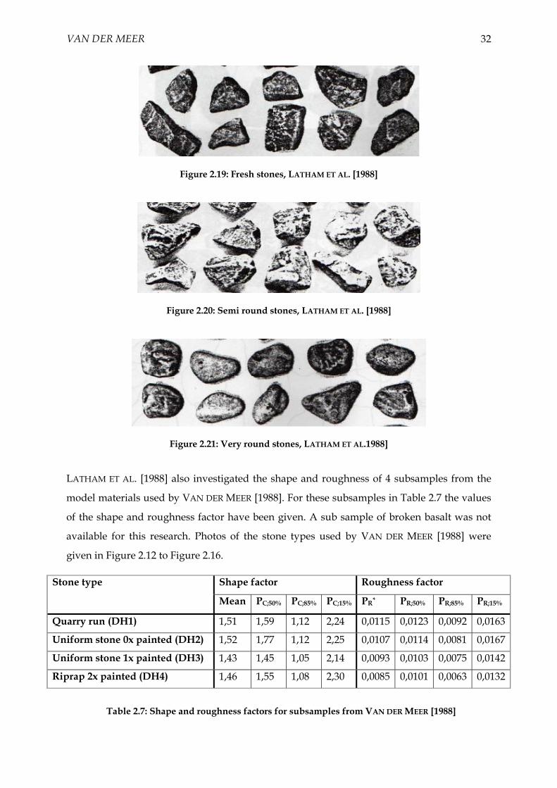
VAN DER MEER 32
Figure 2.19: Fresh stones, LATHAM ET AL. [1988]
Figure 2.20: Semi round stones, LATHAM ET AL. [1988]
Figure 2.21: Very round stones, LATHAM ET AL.1988]
LATHAM ET AL. [1988] also investigated the shape and roughness of 4 subsamples from the
model materials used by VAN DER MEER [1988]. For these subsamples in Table 2.7 the values
of the shape and roughness factor have been given. A sub sample of broken basalt was not
available for this research. Photos of the stone types used by VAN DER MEER [1988] were
given in Figure 2.12 to Figure 2.16.
Shape factor Roughness factor Stone type
Mean PC;50% PC;85% PC;15% PR* PR;50% PR;85% PR;15%
Quarry run (DH1) 1,51 1,59 1,12 2,24 0,0115 0,0123 0,0092 0,0163
Uniform stone 0x painted (DH2) 1,52 1,77 1,12 2,25 0,0107 0,0114 0,0081 0,0167
Uniform stone 1x painted (DH3) 1,43 1,45 1,05 2,14 0,0093 0,0103 0,0075 0,0142
Riprap 2x painted (DH4) 1,46 1,55 1,08 2,30 0,0085 0,0101 0,0063 0,0132
Table 2.7: Shape and roughness factors for subsamples from VAN DER MEER [1988]

VAN DER MEER 33
From these tables it can be seen that the PC values of all subsamples of VAN DER MEER [1988]
strongly correspond to the values of equant stones from LATHAM ET AL. [1988]. Looking at
the roughness factor sub sample DH1 is almost similar to the equant stones of LATHAM ET
AL. [1988]. The roughness of DH2 is somewhere between equant and semi round. DH3 is
most similar to semi round and DH4 is in terms of roughness factor somewhere between
semi round and very round. These findings can be approved by comparing the photos,
however according to the photos sub sample DH4 tends to be much closer to very round
than to semi round.
After deriving shape and roughness parameters LATHAM ET AL. [1988] tested the influence of
these factors on stability. Therefore a model setup was used comparable with the model
setup of VAN DER MEER [1988]. In these tests the damage was measured at N=1000 and
N=3000 waves, while wave height and wave period were varied. To get a clear view on the
influence of roundness and also because of limited flume time a number of parameters were
not varied. Differences between the test conditions of VAN DER MEER [1988] and LATHAM ET
AL. [1988] are mainly based on the fact that it is inappropriate to use sieve sizes in an
investigation to shape effects. Important differences are:
• Armour thickness: LATHAM ET AL. [1988] used a double layer (tarmour ≈ 1,3D50), while
VAN DER MEER [1988] and THOMPSON & SHUTTLER [1975] used tarmour = 2D50.
Another aspect is that for all stone types the armour thickness was calculated using
the D50 of equant stones to avoid different armour thicknesses for each stone type,
because of the varying D50.
• Filter size and thickness: LATHAM ET AL. [1988] used a filter thickness of tfilter ≈
0,43D50 instead of tfilter = 0,5D50. Because of this also the filter size ratio changed was
D50;armour/D50;filter = 5,4 instead of 4,5.
• Placement technique: In LATHAM ET AL. [1988] the stones were placed individually
by hand.
From this the main problem is the validity of the permeability coefficient P, because of the
differences in armour thickness and filter thickness. At first LATHAM ET AL. [1988] used P =
0.1, but during the research it was concluded that a better estimate is P=0.05 to 0.07. Another
problem was that the approach used in LATHAM ET AL. [1988] was based on the assumption
that shape and texture of the stones is independent of all parameters appearing in the

VAN DER MEER 34
formulae of VAN DER MEER [1988]. Unfortunately the permeability depends to some extend
on the shape of the armour stone. This could be seen in the differences in fictitious porosity
(void space expressed as a percentage of the armour layer volume). For the very round rock
the fictitious porosity was 28%, while for the other four stone type values were about 37%.
Also because no tests were done with permeable constructions it could not be proved that for
both permeable (P=0.5) and impermeable (P=0.1) the same effects occur. Therefore the
conclusions from LATHAM ET AL. [1988] can only be applied on impermeable structures
(P=0.1).
Figure 2.22: Pr - cpl and Pr - csu plots from LATHAM ET AL. [1988]: Left P=0,05; right P=0,1
To include the effects of stone shape and roundness LATHAM ET AL. [1988] suggested to
change the values for csurging and cplunging, which makes this effects independent of the other
parameters. To do this in LATHAM ET AL. [1988] 2 plots were made showing the influence of
the asperity roughness PR on cplunging and csurging for P=0.1 and P=0.05 as shown in Figure 2.22.
From these figures a more or less linear relationship can be seen in (averages of) cplunging/PR
and csurging/PR. In the graph with P=0.1 the data points which indicate the subsamples from
VAN DER MEER [1988] are far above the point indicating the test results from LATHAM ET AL.
[1988]. In the graph with P=0.05 the test results from LATHAM ET AL. [1988] for plunging
waves show on average higher values of cplunging. However the test results from LATHAM ET
AL. [1988] for surging waves on average show lower values of csurging than VAN DER MEER
[1988].

VAN DER MEER 35
Assuming a linear relationship from both graphs an average slope for the ratio cplunging/PR
and csurging/PR is derived. After this the lines are extrapolated in such a way that they
intercept the data points of VAN DER MEER [1988]. In this way the effects of stone roundness
can be interpreted on a very simple way by changing the coefficients cplunging and csurging. It
must be mentioned that this analysis is not very accurate because of the low number of tests
and the scattered data.
As compared with standard quarry stone the coefficients in the original formulae of VAN DER
MEER [1988] are changed according to Table 2.8 to include the effects of roundness on
stability. In this table also γ-values are presented which can be used as a multiplier for the
whole equations of VAN DER MEER [1988]. In Table 2.6 only the ratios are given for stones
rounder than the stones used by VAN DER MEER [1988], because for more blockied stones also
the effects of packing has an important role on the stability, which was not investigated by
LATHAM ET AL. [1988].
cplunging γLath;pl csurging γLath;su
Standard Van der Meer 6,20 1,00 1,00 1,00
Semi round (0,009<PR<0,011) 5,89 0,95 1,00 1,00
Very round (PR<0,009) 5,89 0,95 0,80 0,80
Table 2.8: Influence stone roundness on coefficients Van der Meer formulae
With this information the graphs of VAN DER MEER [1988] are redrawn. The stones used in
the tests with different spectra (sub sample DH4 according to LATHAM ET AL. [1988]) with PR
= 0,0087 are indicated as ‘Very Round’, with a factor 0.95 for plunging waves and a factor
0.80 for surging waves.
In Figure 2.23 the influence of including the roundness parameter into is shown by
comparing each graph with the original graph without influence of roundness. It can be seen
that especially for surging waves the impact of including the roundness parameter is huge.
All points that were originally far outside the normal range are nice inside the normal range
in the modified graph. It can be concluded that a rather small deviation in stone roundness
can have large effects on stability.

VAN DER MEER 36
0,0
0,5
1,0
1,5
2,0
0 1 2 3 4 5 6 7 8 9 100,0
0,5
1,0
1,5
2,0
0 1 2 3 4 5 6 7 8 9 10
0,0
0,5
1,0
1,5
2,0
0,0 0,2 0,4 0,6 0,8 1,0 1,2 1,4 1,6
Figure 2.23: Effects of influence stone-roundness on graphs of VAN DER MEER [1988]
γLatham;pl·H2%/∆Dn50 · ξm-1,00,5 · P-0,18 [-]
0,0
0,5
1,0
1,5
2,0
0,0 0,2 0,4 0,6 0,8 1,0 1,2 1,4 1,6
Plunging waves (original graph)
Plunging waves (with influence roundness)
Surging waves (original graph)
Surging waves (with influence roundness)
H2%/∆Dn50 · ξm-1,00,5 · P-0,18 [-]
S/N
0,5 [-
]
H2%/∆Dn50 · ξm-1,0-P · P0,13 · tanα0,5 [-]
S/N
0,5 [-
]
S/N
0,5 [-
]
γLatham;su·H2%/∆Dn50 · ξm-1,0-P · P0,13 · tanα0,5 [-]

VAN DER MEER 37
2.9 New graphs of VAN DER MEER [1988]
With all the adaptations described in the previous sections the graphs are drawn again in
Figure 2.24 and Figure 2.25. In these graphs the correct value of Tm-1,0 and H2% is used and
also the effect of stone roundness is incorporated.
0,0
0,5
1,0
1,5
2,0
0 1 2 3 4 5 6 7 8 9 10
Figure 2.24: New graph for Plunging waves of VAN DER MEER [1988]
In the graph for plunging waves it can be seen that the tests with lower density (Δ=0,92 (light
green) still don’t really correspond to the average test results. They show less damage with
equal wave characteristics than the rest of the tests. On the other hand the large scale tests
(grey) show more damage than the (average) rest of the test results. Also a distinction occurs
between test results with a permeable construction (blue) and test results with an
impermeable construction (yellow, orange and red). It looks like that the test results with
permeable structures (blue) show on average more damage than tests with impermeable
structures.
In the graph for surging waves after correcting for the stone roundness the test results with
narrow and wide spectra (pink) now fit. But strangely some test results in the upper part
don’t really fit. These are test results with permeable structures (blue) and impermeable
structures (yellow).
γLatham;pl·H2%/∆Dn50 · ξm-1,00,5 · P-0,18 [-]
S/N
0,5 [-
]

VAN DER MEER 38
0,0
0,5
1,0
1,5
2,0
0,0 0,2 0,4 0,6 0,8 1,0 1,2 1,4 1,6
Figure 2.25: New graph for surging waves of VAN DER MEER [1988]
With these graphs further on in this M.Sc. Thesis the dataset of VAN DER MEER [1988] will be
compared with the datasets of THOMPSON & SHUTTLER [1975] and VAN GENT ET AL. [2003].
γLatham;su·H2%/∆Dn50 · ξm-1,0-P · P0,13 · tanα0,5 [-]
S/N
0,5 [-
]

39
Chapter 3 THOMPSON & SHUTTLER
THOMPSON & SHUTTLER
3.1 Introduction
The research of THOMPSON & SHUTTLER [1975] was used as a starting point for the work of
VAN DER MEER [1988]. Therefore in this M.Sc. Thesis this dataset will also be analysed and
compared with the datasets of VAN DER MEER [1988] and VAN GENT ET AL. [2003]. To do this
first the data from THOMPSON & SHUTTLER [1975] had to be entered in the spreadsheet,
because no digital data was available.
3.2 Damage level
The damage level in the dataset of THOMPSON & SHUTTLER [1975] is written as NΔ. This
parameter has to be rewritten to the damage level, S, used in the dataset of VAN DER MEER
[1988]. For the dataset of THOMPSON & SHUTTLER [1975] the ratio Dn50/D50 is 0,82 according
to VAN DER MEER [1988]. In Table 3.1 the conversion is made from NΔ to S using the
following formula.
SD
AD
AD
DAN
a
b
na
b
a
b
a
b ⋅⋅⋅
=⋅⋅⋅=⋅⋅=⋅⋅
⋅⋅=Δ ρ
ρπρ
ρπρ
ρππρ
ρ 2
250
2
250
350
50 82,054182,054
6
9
6
9

THOMPSON & SHUTTLER 40
D50
[m]
ρb
[kg/m3]
ρa
[kg/m3]
ρb/ρa
[-]
0,020 1510 2700 0,559259259 S=NΔ/6,463753336
0,030 1480 2700 0,548148148 S=NΔ/6,335334395
0,040 1480 2700 0,548148148 S=NΔ/6,335334395
Table 3.1: Conversion from NΔ to S
In order to make a comparison between the data of THOMPSON & SHUTTLER [1975], the data
of VAN DER MEER [1988] and VAN GENT ET AL. [2003] the dataset of THOMPSON & SHUTTLER
[1975] also has to be entered in the spreadsheet and transformed.
3.3 Correctness spreadsheet
After the conversion in Figure 3.1 and Figure 3.2 the dataset of THOMPSON & SHUTTLER
[1975] is drawn together with the original dataset of VAN DER MEER [1988]. On the
background the original graphs from the doctoral thesis of VAN DER MEER [1988] are given in
which the dataset of THOMPSON & SHUTTLER [1975] was also included.
Figure 3.1: THOMPSON & SHUTTLER [1975] and VAN DER MEER [1988] for plunging waves
0,0
0,1
0,2
0,3
0,4
0,5
0,6
0,7
1 2 3 4 5 6 7
Hs/∆Dn50 · ξm0,5 · P-0,18 [-]
S/N
0,5 [-
]

THOMPSON & SHUTTLER 41
Besides the differences in the dataset of VAN DER MEER [1988] that were described before, no
noteworthy differences between the original graph of VAN DER MEER [1988] and the new
graph can be seen in Figure 3.1. Small differences can occur because of scaling effects due to
the document scanning of small round off errors.
In Figure 3.2 a few deviating points, indicated with red circles, in the dataset of THOMPSON &
SHUTTLER [1975] can be seen. Probably in VAN DER MEER [1988] again some mistakes were
made with the critical Iribarren parameter, ξc. The reason why these deviations cannot be
found the graph for plunging waves is that this graph is has very dense areas in which
individual points are hard to distinguish.
Figure 3.2: THOMPSON & SHUTTLER [1975] and VAN DER MEER [1988] for surging waves
0,0
0,1
0,2
0,3
0,4
0,5
0,6
0,7
0,2 0,3 0,4 0,5 0,6 0,7 0,8 0,9 1,0
Hs/∆Dn50 · ξm-P · P0,13 · tanα0,5 [-]
S/N
0,5 [-
]

THOMPSON & SHUTTLER 42
3.4 Conversion dataset to Tm-1,0 and H2% values
After this all parameters need to be written in the same format as the dataset of VAN GENT ET
AL. [2003]. In this way a clear comparison of the datasets can be made. This means that the
dataset of THOMPSON & SHUTTLER [1975] also has to be rewritten in terms of H2% and Tm-1,0.
3.4.1 Wave height
In the dataset of THOMPSON & SHUTTLER [1975] the wave height is given in H3. This is
another notation for the significant wave height, Hs. In order to rewrite this wave height to
the wave height exceeded by 2% of the waves, H2%, the point model of BATTJES &
GROENENDIJK [2000] can be used.
For Rayleigh distributed waves the significant wave height estimated from the wave
spectrum, Hm0, can be calculated with the following approximation.
00 ...005,4 mH m ⋅=
Real time wave observations by LONGUET & HIGGINS [1980] and numerical simulations by
GODA [1988] show that the significant wave height measured from a zero crossing analysis,
H1/3, may be 5% to 10% lower than the significant wave height as estimated from the
spectrum. GODA [1988] suggests H1/3 = 0,95Hm0, which results in:
03/1 804,3 mH ⋅=
When the zero-th order spectral moment is known the root-mean-square wave height, Hrms,
of each test can be calculated. With this Hrms the transitional wave height, Htr, is normalised
to the normalised transitional wave height as described in paragraph A1.
In table 2 of BATTJES & GROENENDIJK [2000] the characteristic normalised wave heights are
given as a function of the normalised transitional wave height, trH~ . Out of this table the ratio
H2%/H1/3 can be calculated.
Using this approach for all tests of the dataset of THOMPSON & SHUTTLER [1975] the ratio
H2%/Hs has been calculated. The spreadsheet shows that for all tests the ratio H2%/H1/3 is
equal to 1,4.

THOMPSON & SHUTTLER 43
3.4.2 Wave period
According to INFRAM, I489 [2001] the ratio Tm-1,0/Tp is equal to 1,1, in which the peak
period, Tp, is calculated from the mean period, Tm, using Tp = 1,15Tm.
3.5 New graphs of dataset THOMPSON & SHUTTLER [1975]
Because no specific details are known about the stones used by THOMPSON & SHUTTLER
[1975] it is assumed that the stones used in this research are of the standard type which was
also used by VAN DER MEER [1988]. Therefore no correction factors are needed for this
dataset. With these adaptations the datasets of THOMPSON & SHUTTLER [1975] are drawn
again in Figure 3.3 and Figure 3.4.
0,0
0,5
1,0
1,5
2,0
0 1 2 3 4 5 6 7 8 9 10
Figure 3.3: Plunging waves THOMPSON & SHUTTLER [1975]
γLatham;pl·H2%/∆Dn50 · ξm-1,00,5 · P-0,18 [-]
S/N
0,5 [-
]

THOMPSON & SHUTTLER 44
0,0
0,5
1,0
1,5
2,0
0,0 0,2 0,4 0,6 0,8 1,0 1,2 1,4 1,6
Figure 3.4: Surging waves THOMPSON & SHUTTLER [1975]
With these graphs the dataset of THOMPSON & SHUTTLER [1975] will be compared with the
datasets of VAN DER MEER [1988] and VAN GENT ET AL. [2003] in Chapter 5.
γLatham;su·H2%/∆Dn50 · ξm-1,0-P · P0,13 · tanα0,5 [-]
S/N
0,5 [-
]

45
Chapter 4 VAN GENT
VAN GENT
4.1 Introduction
Before the dataset of VAN GENT ET AL. [2003] can be compared with the datasets of
THOMPSON & SHUTTLER [1975] and VAN DER MEER [1988] the dataset of VAN GENT ET AL.
[2003] had to be entered in an Excel spreadsheet. Because only graphs from the dataset of
VAN GENT ET AL. [2003] were available during this M.Sc. Thesis the data was read from the
graphs and entered in the spreadsheet to be able to compare the data likewise.
4.2 Correctness spreadsheet
Using the original graphs of VAN GENT ET AL. [2003] the correctness of the spreadsheet
checked. In Figure 4.1 the graph for plunging waves is plotted (in grey) with on the
background original graph from VAN GENT ET AL. [2003]. In the same way the graph for
surging waves is treated. In Figure 4.2 the graph for surging waves is plotted together with
the original graph from VAN GENT [2003]. With these graphs the dataset of VAN GENT ET
AL. [2003] is compared with the datasets of VAN DER MEER [1988] and THOMPSON &
SHUTTLER [1975]. No corrections or changes were made to the dataset of VAN GENT ET AL.
[2003], which also means that the assumption is made that the stones used are of the
standard stone type (γLatham = 1,0).

VAN GENT 46
Figure 4.1: Plunging waves, reconstructed graph (grey), original graph (VAN GENT ET AL. [2003])
Figure 4.2: Surging waves, reconstructed graph (grey), original graph VAN GENT ET AL. [2003]
γLatham;su·H2%/∆Dn50 · ξm-1,0-P · P0,13 · tanα0,5 [-]
S/N
0,5 [-
]
0
0,2
0,4
0,6
0,8
1
1,2
1,4
1,6
1,8
2
0 0,1 0,2 0,3 0,4 0,5 0,6 0,7 0,8 0,9 1 1,1 1,2 1,3 1,4 1,5 1,6
γLatham;pl·H2%/∆Dn50 · ξm-1,00,5 · P-0,18 [-]
S/N
0,5 [-
]
0
0,2
0,4
0,6
0,8
1
1,2
1,4
1,6
1,8
2
0 1 2 3 4 5 6 7 8 9 10

47
Chapter 5 COMPARISON OF DATASETS
COMPARISON OF DATASETS
5.1 Plunging waves
In Figure 5.1 to Figure 5.4 the graphs of VAN DER MEER [1988] (red), THOMPSON & SHUTTLER
[1975] (green) and VAN GENT ET AL. [2003] (blue) have been plotted together.
0,0
0,5
1,0
1,5
2,0
0 1 2 3 4 5 6 7 8 9 10
Figure 5.1: Plunging waves: THOMPSON & SHUTTLER [1975] (green), VAN DER MEER [1988] (red), VAN GENT ET AL. [2003] (blue
γLatham;pl·H2%/∆Dn50 · ξm-1,00,5 · P-0,18 [-]
S/N
0,5 [-
]

COMPARISON OF DATASETS 48
0,0
0,5
1,0
1,5
2,0
0 1 2 3 4 5 6 7 8 9 10
Figure 5.2: Plunging waves: VAN DER MEER [1988] (red), VAN GENT ET AL. [2003] (blue)
0,0
0,5
1,0
1,5
2,0
0 1 2 3 4 5 6 7 8 9 10
Figure 5.3: Plunging waves: THOMPSON & SHUTTLER [1975] (green), VAN GENT ET AL. [2003] (blue)
γLatham;pl·H2%/∆Dn50 · ξm-1,00,5 · P-0,18 [-]
S/N
0,5 [-
]
γLatham;pl·H2%/∆Dn50 · ξm-1,00,5 · P-0,18 [-]
S/N
0,5 [-
]

COMPARISON OF DATASETS 49
0,0
0,5
1,0
1,5
2,0
0 1 2 3 4 5 6 7 8 9 10
Figure 5.4: Plunging waves: THOMPSON & SHUTTLER [1975] (green), VAN DER MEER [1988] (red)
In the graphs for plunging waves the datasets still don’t really correspond to each other. The
dataset of VAN GENT ET AL. [2003] still tends to show more damage than the datasets of VAN
DER MEER [1988] and THOMPSON & SHUTTLER [1975]. The datasets of VAN DER MEER [1988]
and THOMPSON & SHUTTLER [1975] however show a similar trend.
5.2 Surging waves
Subsequently in Figure 5.5 to Figure 5.8 the graphs of VAN DER MEER [1988] (red), THOMPSON
& SHUTTLER [1975] (green) and VAN GENT ET AL. [2003] (blue) have been plotted together.
Also in these graphs a certain distinction between the data of VAN GENT ET AL. [2003] and
the data of VAN DER MEER [1988] and THOMPSON & SHUTTLER [1975] can be seen.
γLatham;pl·H2%/∆Dn50 · ξm-1,00,5 · P-0,18 [-]
S/N
0,5 [-
]

COMPARISON OF DATASETS 50
0,0
0,5
1,0
1,5
2,0
0,0 0,2 0,4 0,6 0,8 1,0 1,2 1,4 1,6
Figure 5.5: Surging waves: THOMPSON & SHUTTLER [1975] (green), VAN DER MEER [1988] (red), VAN GENT ET AL. [2003] (blue)
0,0
0,5
1,0
1,5
2,0
0,0 0,2 0,4 0,6 0,8 1,0 1,2 1,4 1,6
Figure 5.6: Surging waves: VAN DER MEER [1988] (red), VAN GENT ET AL. [2003] (blue) γLatham;su·H2%/∆Dn50 · ξm-1,0
-P · P0,13 · tanα0,5 [-]
S/N
0,5 [-
]
γLatham;su·H2%/∆Dn50 · ξm-1,0-P · P0,13 · tanα0,5 [-]
S/N
0,5 [-
]

COMPARISON OF DATASETS 51
0,0
0,5
1,0
1,5
2,0
0,0 0,2 0,4 0,6 0,8 1,0 1,2 1,4 1,6
Figure 5.7: Surging waves: THOMPSON & SHUTTLER [1975] (green), VAN GENT ET AL. [2003] (blue)
0,0
0,5
1,0
1,5
2,0
0,0 0,2 0,4 0,6 0,8 1,0 1,2 1,4 1,6
Figure 5.8: Surging waves: THOMPSON & SHUTTLER [1975] (green), VAN DER MEER [1988] (red) γLatham;su·H2%/∆Dn50 · ξm-1,0
-P · P0,13 · tanα0,5 [-]
S/N
0,5 [-
]
γLatham;su·H2%/∆Dn50 · ξm-1,0-P · P0,13 · tanα0,5 [-]
S/N
0,5 [-
]
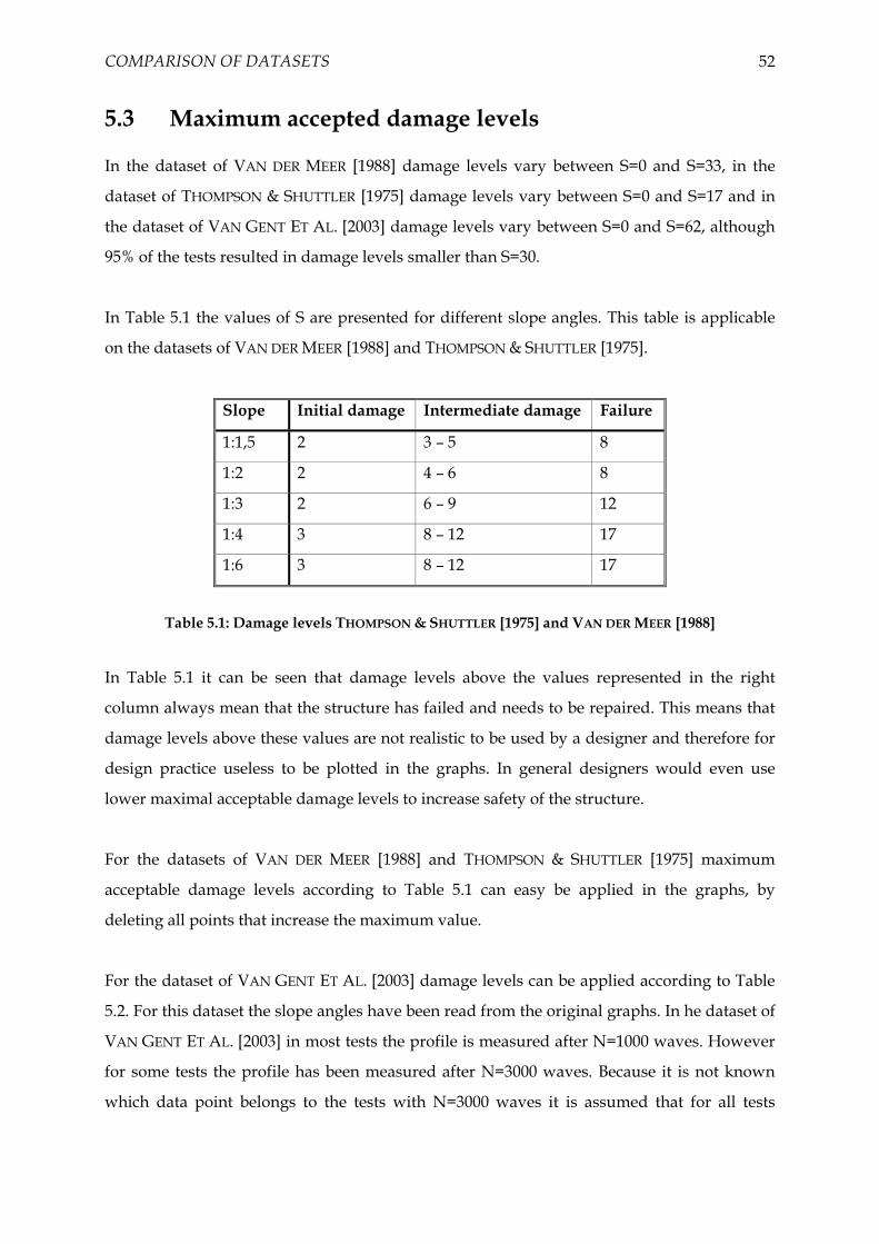
COMPARISON OF DATASETS 52
5.3 Maximum accepted damage levels
In the dataset of VAN DER MEER [1988] damage levels vary between S=0 and S=33, in the
dataset of THOMPSON & SHUTTLER [1975] damage levels vary between S=0 and S=17 and in
the dataset of VAN GENT ET AL. [2003] damage levels vary between S=0 and S=62, although
95% of the tests resulted in damage levels smaller than S=30.
In Table 5.1 the values of S are presented for different slope angles. This table is applicable
on the datasets of VAN DER MEER [1988] and THOMPSON & SHUTTLER [1975].
Slope Initial damage Intermediate damage Failure
1:1,5 2 3 – 5 8
1:2 2 4 – 6 8
1:3 2 6 – 9 12
1:4 3 8 – 12 17
1:6 3 8 – 12 17
Table 5.1: Damage levels THOMPSON & SHUTTLER [1975] and VAN DER MEER [1988]
In Table 5.1 it can be seen that damage levels above the values represented in the right
column always mean that the structure has failed and needs to be repaired. This means that
damage levels above these values are not realistic to be used by a designer and therefore for
design practice useless to be plotted in the graphs. In general designers would even use
lower maximal acceptable damage levels to increase safety of the structure.
For the datasets of VAN DER MEER [1988] and THOMPSON & SHUTTLER [1975] maximum
acceptable damage levels according to Table 5.1 can easy be applied in the graphs, by
deleting all points that increase the maximum value.
For the dataset of VAN GENT ET AL. [2003] damage levels can be applied according to Table
5.2. For this dataset the slope angles have been read from the original graphs. In he dataset of
VAN GENT ET AL. [2003] in most tests the profile is measured after N=1000 waves. However
for some tests the profile has been measured after N=3000 waves. Because it is not known
which data point belongs to the tests with N=3000 waves it is assumed that for all tests

COMPARISON OF DATASETS 53
N=1000. This is a safe assumption for the upper boundary, because the value of S/N0,5 will
only decrease when N=3000 would be applied.
Slope Initial damage Failure
1:2 2 8
1:4 2 17
Table 5.2: Damage levels VAN GENT ET AL. [2003]
Finally in Figure 5.9 and Figure 5.10 the graphs are plotted with the use of maximum
damage levels. To be able to make a good comparison in these graphs on both axes the same
scales are used as in the graphs in Figure 5.1 to Figure 5.8. In paragraph 5.4 and 5.5 the
graphs are plotted on a more detailed scale.
0,0
0,5
1,0
1,5
2,0
0 1 2 3 4 5 6 7 8 9 10
Figure 5.9: Plunging waves: THOMPSON & SHUTTLER [1975] (green), VAN DER MEER [1988] (red), VAN GENT ET AL. [2003] (blue) with maximal acceptable damage levels
γLatham;pl·H2%/∆Dn50 · ξm-1,00,5 · P-0,18 [-]
S/N
0,5 [-
]
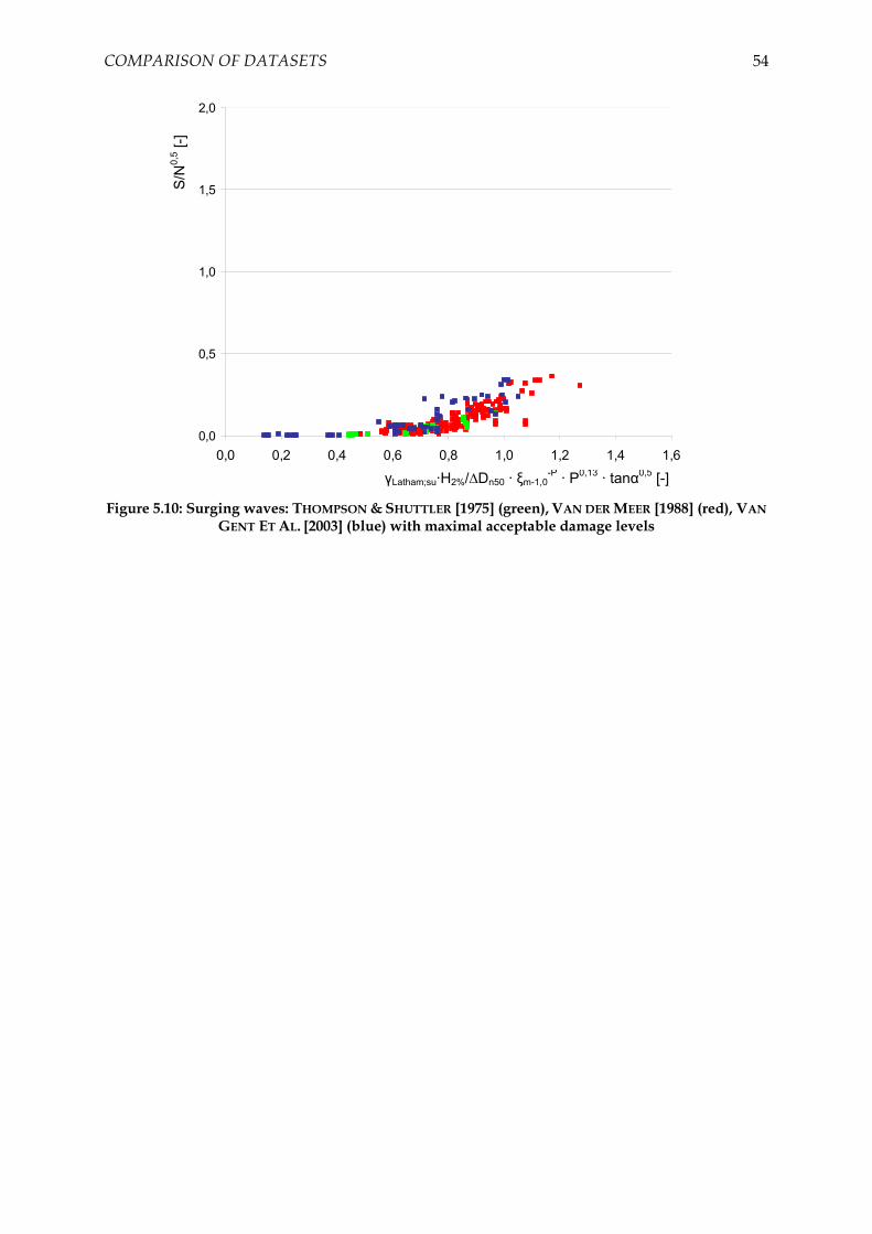
COMPARISON OF DATASETS 54
0,0
0,5
1,0
1,5
2,0
0,0 0,2 0,4 0,6 0,8 1,0 1,2 1,4 1,6
Figure 5.10: Surging waves: THOMPSON & SHUTTLER [1975] (green), VAN DER MEER [1988] (red), VAN GENT ET AL. [2003] (blue) with maximal acceptable damage levels
γLatham;su·H2%/∆Dn50 · ξm-1,0-P · P0,13 · tanα0,5 [-]
S/N
0,5 [-
]

COMPARISON OF DATASETS 55
5.4 Detailed graphs for plunging waves
In Figure 5.11 and FigureA.6 (Appendix E) again the graphs of VAN DER MEER [1988],
THOMPSON & SHUTTLER [1975] and VAN GENT ET AL. [2003] are plotted together.
0,0
0,1
0,2
0,3
0,4
0,5
0,6
0,7
0 1 2 3 4 5 6 7 8 9 10
Figure 5.11: Plunging waves: THOMPSON & SHUTTLER [1975] (green), VAN DER MEER [1988] (red), VAN GENT ET AL. [2003] (blue) with maximal acceptable damage levels
0,0
0,1
0,2
0,3
0,4
0,5
0,6
0,7
0 1 2 3 4 5 6 7 8 9 10
Figure 5.12: Plunging waves: 5% and 95% Exceedance lines, THOMPSON & SHUTTLER [1975] (green), VAN DER MEER [1988] (red), VAN GENT ET AL. [2003] (blue)
γLatham;pl·H2%/∆Dn50 · ξm-1,00,5 · P-0,18 [-]
S/N
0,5 [-
]
γLatham;pl·H2%/∆Dn50 · ξm-1,00,5 · P-0,18 [-]
S/N
0,5 [-
]

COMPARISON OF DATASETS 56
In Figure 5.12 the 5%- and 95%-exceedance lines of the datasets of VAN DER MEER [1988],
THOMPSON & SHUTTLER [1975] and VAN GENT ET AL. [2003] have been plot for plunging
waves. Figure 5.11 and Figure 5.12 again show the differences between the dataset of VAN
GENT ET AL. [2003] and the datasets of VAN DER MEER [1988] and THOMPSON & SHUTTLER
[1975]. The 5%-exceedance line of the dataset of VAN GENT ET AL. [2003] is on the whole
range of the graph higher than those of VAN DER MEER [1988] and THOMPSON & SHUTTLER
[1975].
5.5 Detailed graphs for surging waves
Also for surging waves in Figure 5.13 and FigureA.7 (Appendix E) the graphs have been
plotted on a detailed scale and in Figure 5.14 the 5%- and 95%-exceedance lines have been
plotted.
0,0
0,1
0,2
0,3
0,4
0,5
0,6
0,7
0,0 0,1 0,2 0,3 0,4 0,5 0,6 0,7 0,8 0,9 1,0 1,1 1,2 1,3
Figure 5.13: Surging waves: THOMPSON & SHUTTLER [1975] (green), VAN DER MEER [1988] (red), VAN GENT ET AL. [2003] (blue) with maximal acceptable damage levels
γLatham;su·H2%/∆Dn50 · ξm-1,0-P · P0,13 · tanα0,5 [-]
S/N
0,5 [-
]

COMPARISON OF DATASETS 57
0,0
0,1
0,2
0,3
0,4
0,5
0,6
0,7
0,1 0,2 0,3 0,4 0,5 0,6 0,7 0,8 0,9 1,0 1,1 1,2 1,3
Figure 5.14: Surging waves: 5% and 95% Exceedance lines, THOMPSON & SHUTTLER [1975] (green), VAN DER MEER [1988] (red), VAN GENT ET AL. [2003] (blue)
In Figure 5.14 it can be seen that also for surging waves the 5% exceedance line of the dataset
of VAN GENT ET AL. [2003] is higher than the 5% exceedance lines of VAN DER MEER [1988]
and THOMPSON & SHUTTLER [1975].
Although differences can be seen on both graphs for plunging and surging waves it must be
remarked that the correct use of the maximum damage levels in the dataset of VAN GENT ET
AL. [2003] could imply a downward shift of the 5% exceedance line (upper blue line). In this
a correct use of the maximum damage levels means the use of N=3000 in determining the
maximum damage level S/N0,5 for those tests in which the profile was measured after
N=3000 waves.
γLatham;su·H2%/∆Dn50 · ξm-1,0-P · P0,13 · tanα0,5 [-]
S/N
0,5 [-
]

58
Chapter 6 STATISTICS
STATISTICS
6.1 Introduction
In the previous chapter it could be concluded that differences appear between the datasets of
VAN GENT ET AL. [2003], VAN DER MEER [1988] and THOMPSON & SHUTTLER [1975]. In this
chapter the datasets will be compared on a statistical way.
6.2 Basic statistics for plunging waves
Before a detailed statistic investigation can be done first basic statistical values have to be
determined of the datasets. With a step size of 0,5 on the horizontal axis the mean, standard
deviation, minimum, maximum, band width, 5%- and 95%-exceedance values and the
number of tests per step were determined from the datasets of VAN GENT ET AL. [2003], VAN
DER MEER [1988] and THOMPSON & SHUTTLER [1975]. These values are presented in Table 6.1.
In Figure 6.1 and Figure 6.2 the mean and the standard deviation have been plotted.

STATISTICS 59
Dataset VAN DER MEER [1988] S/N0,5 γLatham;pl·H2%/∆Dn50 · ξm-1,00,5 · P-0,18
Mean Sd. Min. Max. Band width 95% 5% Nr. 4,25 0,031 0,011 0,016 0,050 0,035 0,01 0,05 16 4,75 0,055 0,026 0,023 0,126 0,103 0,01 0,10 24 5,25 0,077 0,032 0,031 0,163 0,132 0,02 0,13 39 5,75 0,118 0,043 0,000 0,254 0,254 0,05 0,19 53 6,25 0,159 0,066 0,058 0,374 0,316 0,05 0,27 50 6,75 0,197 0,053 0,072 0,306 0,234 0,11 0,28 41 7,25 0,277 0,065 0,172 0,369 0,197 0,17 0,38 18 7,75 0,296 0,135 0,110 0,511 0,401 0,07 0,52 17 8,25 0,367 0,131 0,192 0,476 0,284 0,15 0,58 4 8,75 0,351 0,190 0,216 0,485 0,269 0,04 0,66 2
Dataset VAN GENT ET AL. [2003] S/N0,5 γLatham;pl·H2%/∆Dn50 · ξm-1,00,5 · P-0,18
Mean Sd. Min. Max. Band width 95% 5% Nr. 4,25 0,020 0,007 0,012 0,029 0,017 0,01 0,03 4 4,75 0,126 0,018 0,100 0,150 0,050 0,10 0,16 5 5,25 0,141 0,080 0,062 0,310 0,248 0,01 0,27 10 5,75 0,171 0,068 0,035 0,340 0,305 0,06 0,28 28 6,25 0,235 0,091 0,062 0,375 0,313 0,09 0,39 17 6,75 0,308 0,082 0,170 0,420 0,250 0,17 0,44 14 7,25 0,351 0,121 0,130 0,505 0,375 0,15 0,55 11 7,75 0,508 0,004 0,505 0,510 0,005 0,50 0,51 2
Dataset THOMPSON & SHUTTLER [1975] S/N0,5 γLatham;pl·H2%/∆Dn50 · ξm-1,00,5 · P-0,18
Mean Sd. Min. Max. Band width 95% 5% Nr. 2,75 0,011 0,004 0,005 0,018 0,013 0,00 0,02 8 3,25 0,011 0,012 0,001 0,047 0,047 -0,01 0,03 20 3,75 0,023 0,012 0,003 0,043 0,040 0,00 0,04 28 4,25 0,032 0,013 0,013 0,065 0,052 0,01 0,05 28 4,75 0,041 0,012 0,019 0,071 0,052 0,02 0,06 30 5,25 0,070 0,023 0,026 0,158 0,132 0,03 0,11 40 5,75 0,115 0,045 0,052 0,241 0,189 0,04 0,19 29 6,25 0,134 0,046 0,058 0,263 0,205 0,06 0,21 22 6,75 0,215 0,052 0,121 0,294 0,173 0,13 0,30 11 7,25 0,216 0,087 0,117 0,299 0,182 0,07 0,36 4 7,75 0,304 0,073 0,232 0,377 0,145 0,18 0,42 3
Table 6.1: Basic statistical values for plunging waves

STATISTICS 60
0,00
0,10
0,20
0,30
0,40
0,50
0,60
0,70
0 1 2 3 4 5 6 7 8 9 10
Van der MeerVan GentThompson&Shuttler
Figure 6.1: Mean values (step size 0,5) for plunging waves
0,00
0,02
0,04
0,06
0,08
0,10
0,12
0,14
0,16
0,18
0,20
0 1 2 3 4 5 6 7 8 9 10
Van der MeerVan GentThompson&Shuttler
Figure 6.2: Standard deviation (step size 0,5) for plunging waves
In Figure 6.1 it can be seen that the mean values of S/N0,5 of the dataset of VAN GENT ET AL.
[2003] are higher than those of the datasets of VAN DER MEER [1988] and THOMPSON &
SHUTTLER [1975]. In Figure 6.2 it can be seen that on average the values of the standard
deviation of the dataset of VAN GENT ET AL. [2003] are higher than those of the datasets of
VAN DER MEER [1988] and THOMPSON & SHUTTLER [1975].
γLatham;pl·H2%/∆Dn50 · ξm-1,00,5 · P-0,18 [-]
S/N
0,5 [-
]
γLatham;pl·H2%/∆Dn50 · ξm-1,00,5 · P-0,18 [-]
S/N
0,5 [-
]

STATISTICS 61
6.3 Basic statistics for surging waves
In the same way in Table 6.2. basic statistic values have been determined for the tests with
surging waves. For surging waves on the horizontal axis the step size is 0,1.
Dataset VAN DER MEER [1988] S/N0,5
γLath·H2%/∆Dn50·ξm-1,0-P·P0,13·tanα0,5 Mean Sd. Min. Max. Band width 95% 5% Nr. 0,55 0,032 0,019 0,013 0,076 0,063 0,00 0,06 10 0,65 0,032 0,013 0,008 0,062 0,054 0,01 0,05 40 0,75 0,056 0,029 0,010 0,163 0,152 0,01 0,10 52 0,85 0,112 0,046 0,038 0,239 0,201 0,04 0,19 42 0,95 0,152 0,042 0,065 0,222 0,157 0,08 0,22 36 1,05 0,257 0,073 0,149 0,324 0,175 0,14 0,38 7 1,15 0,344 0,015 0,333 0,361 0,028 0,32 0,37 3 1,25 0,306 0,306 0,306 0,000 1
Dataset VAN GENT ET AL. [2003] S/N0,5
γLath·H2%/∆Dn50·ξm-1,0-P·P0,13·tanα0,5 Mean Sd. Min. Max. Band width 95% 5% Nr.
0,15 0,002 0,004 0,000 0,010 0,010 -0,01 0,01 5 0,25 0,000 0,000 0,000 0,000 0,000 5 0,35 0,000 0,000 0,000 0,000 0,000 3 0,45 0,000 0,000 0,000 0,000 1 0,55 0,055 0,055 0,055 0,000 1 0,65 0,040 0,018 0,010 0,060 0,050 0,01 0,07 11 0,75 0,096 0,073 0,020 0,235 0,215 -0,02 0,22 13 0,85 0,204 0,027 0,160 0,225 0,065 0,16 0,25 5 0,95 0,220 0,068 0,130 0,310 0,180 0,11 0,33 6 1,05 0,279 0,072 0,200 0,340 0,140 0,16 0,40 4 1,15 0,002 0,004 0,000 0,010 0,010 -0,01 0,01 5
Dataset THOMPSON & SHUTTLER [1975] S/N0,5
γLath·H2%/∆Dn50·ξm-1,0-P·P0,13·tanα0,5 Mean Sd. Min. Max. Band width 95% 5% Nr. 0,45 0,004 0,004 0,000 0,012 0,012 0,00 0,01 6 0,55 0,007 0,004 0,004 0,010 0,006 0,00 0,01 2 0,65 0,010 0,007 0,003 0,018 0,015 0,00 0,02 4 0,75 0,047 0,016 0,020 0,063 0,043 0,02 0,07 6 0,85 0,077 0,022 0,044 0,106 0,062 0,04 0,11 6 0,95 0,134 0,134 0,134 0,000 1
Table 6.2: Basic statistical values for surging waves

STATISTICS 62
For surging waves the mean and the standard deviation have been plotted in Figure 6.3 and
Figure 6.4.
0,00
0,05
0,10
0,15
0,20
0,25
0,30
0,35
0,40
0 0,2 0,4 0,6 0,8 1 1,2 1,4
Van der MeerVan GentThompson&Shuttler
Figure 6.3: Mean values (step size 0,1) for surging waves
0,00
0,01
0,02
0,03
0,04
0,05
0,06
0,07
0,08
0 0,2 0,4 0,6 0,8 1 1,2 1,4
Van der MeerVan GentThompson&Shuttler
Figure 6.4: Standard deviation (step size 0,1) for surging waves
γLatham;su·H2%/∆Dn50 · ξm-1,0-P · P0,13 · tanα0,5 [-]
S/N
0,5 [-
]
γLatham;su·H2%/∆Dn50 · ξm-1,0-P · P0,13 · tanα0,5 [-]
S/N
0,5 [-
]

STATISTICS 63
Figure 6.3 shows that also for surging waves the mean of the dataset of VAN GENT ET AL.
[2003] is higher than the mean of VAN DER MEER [1988] and THOMPSON & SHUTTLER [1975].
In Figure 6.4 it can be seen that the standard deviation of the dataset of VAN GENT ET AL.
[2003] increases to quite high values in the first part of the graph, where after it decreases to
values comparable to those of the dataset of VAN DER MEER [1988].
6.4 The T-test
To test whether the datasets of VAN GENT ET AL. [2003], VAN DER MEER [1988] and
THOMPSON & SHUTTLER R [1975] are statistically different the T-test will be used. The T-test is
described in Appendix A4 . For the T-test a on the horizontal axis a step size of 0,5 is taken
for plunging waves and a step size of 0,1 is taken for surging waves. For each step the
datasets were compared. For all results a confidence level of 95% is applied.
6.4.1 VAN GENT ET AL. [2003] – VAN DER MEER [1988]
The first datasets to be statistically compared with the T-test are the datasets of VAN GENT ET
AL. [2003] and VAN DER MEER [1988]. The results of the T-test for these datasets are given in
Table 6.3 and Table 6.4.
γLatham;pl·H2%/∆Dn50 · ξm-1,00,5 · P-0,18 tobs dof t*95% T-test
4,25 -2,64 18 1,33 Significant different 4,75 7,33 27 1,31 Significant different 5,25 2,45 47 1,30 Significant different 5,75 3,76 79 1,29 Significant different 6,25 3,19 65 1,30 Significant different 6,75 4,71 53 1,30 Significant different 7,25 1,88 27 1,31 Significant different 7,75 6,43 17 1,33 Significant different
Table 6.3: The T-test for VAN GENT ET AL. [2003] and VAN DER MEER [1988] for plunging waves

STATISTICS 64
γLath·H2%/∆Dn50·ξm-1,0-P·P0,13·tanα0,5 tobs dof t*95% T-test
0,65 1,36 49 1,30 Significant different 0,75 1,91 63 1,30 Significant different 0,85 6,59 45 1,30 Significant different 0,95 2,40 40 1,30 Significant different 1,05 0,48 9 1,38
Table 6.4: The T-test for VAN GENT ET AL. [2003] and VAN DER MEER [1988] for surging waves
From Table 6.3 and Table 6.4 it can be concluded that the datasets of VAN DER MEER [1988]
and VAN GENT ET AL. [2003] are statistically significant different both for plunging and
surging waves.
6.4.2 THOMPSON & SHUTTLER [1975] - VAN DER MEER [1988]
Subsequently the results of the T-tests for the comparison of the datasets of VAN DER MEER
[1988] and THOMPSON & SHUTTLER [1975] are shown in Table 6.5 and Table 6.6.
γLatham;pl·H2%/∆Dn50 · ξm-1,00,5 · P-0,18 tobs dof t*95% T-test
4,25 -0,13 42 1,30 4,75 2,37 52 1,30 Significant different 5,25 1,07 77 1,29 5,75 0,25 80 1,29 6,25 1,81 70 1,29 Significant different 6,75 -0,96 50 1,30 7,25 1,33 20 1,33 Significant different 7,75 -0,15 18 1,33
Table 6.5: The T-test for THOMPSON & SHUTTLER [1975] and VAN DER MEER [1988]
γLath·H2%/∆Dn50·ξm-1,0-P·P0,13·tanα0,5 tobs dof t*95% T-test
0,55 3,85 10 1,37 Significant different 0,65 5,56 42 1,30 Significant different 0,75 1,24 56 1,30 0,85 3,15 46 1,30 Significant different
Table 6.6: The T-test for THOMPSON & SHUTTLER [1975] and VAN DER MEER [1988] for surging waves

STATISTICS 65
From Table 6.5 and Table 6.6 it can be concluded that for plunging waves the datasets of
VAN DER MEER [1988] and THOMPSON & SHUTTLER [1975] not significantly different on most
points. For surging waves however the datasets are significantly different on 3 out of 4
points.
6.4.3 THOMPSON & SHUTTLER [1975] - VAN GENT ET AL. [2003]
The results of the T-tests for the comparison of the datasets of THOMPSON & SHUTTLER [1975]
and VAN GENT ET AL. [2003] are shown in Table 6.7 and Table 6.8.
γLatham;pl·H2%/∆Dn50 · ξm-1,00,5 · P-0,18 tobs dof t*95% T-test
4,25 -2,79 30 1,31 Significant different 4,75 10,08 33 1,31 Significant different 5,25 2,74 48 1,30 Significant different 5,75 3,62 55 1,30 Significant different 6,25 4,18 37 1,31 Significant different 6,75 3,45 23 1,32 Significant different 7,25 2,39 13 1,35 Significant different 7,75 4,85 3 1,64 Significant different
Table 6.7: The T-test for THOMPSON & SHUTTLER [1975] and VAN GENT ET AL. [2003]
γLath·H2%/∆Dn50·ξm-1,0-P·P0,13·tanα0,5 tobs dof t*95% T-test
0,65 -4,66 13 1,4 Significant different 0,75 -2,31 17 1,3 Significant different 0,85 -8,59 9 1,4 Significant different
Table 6.8: The T-test for THOMPSON & SHUTTLER [1975] and VAN GENT ET AL. [2003] for surging waves
In Table 6.7 and Table 6.8 it can be seen that for plunging and surging waves the datasets of
THOMPSON & SHUTTLER [1975] and VAN GENT ET AL. [2003] are on all points significantly
different.

66
Chapter 7 DESIGN PRACTICE
DESIGN PRACTICE
7.1 Introduction
In design practise usually the maximum damage level is used as an input parameter. The
maximum accepted damage level depends on how much damage the designer of the
breakwater allows on the breakwater. The choice of a damage level strongly depends on the
chosen safety level and available finances. Other input parameters are the wave height,
permeability, slope angle, wave period (in ξ) and the number of waves. This means that the
only real output parameter is the stone diameter.
For some reason the graphs which have been described before are always presented with the
diameter on the horizontal axis and the damage level in the vertical axis. When designing a
breakwater in general the designer has a given maximum damage level and is interested in a
corresponding stone diameter. Therefore is would be easier to draw the graphs on the other
way around. This is done in Figure 7.1 for plunging waves and in Figure 7.2 for surging
waves.

DESIGN PRACTICE 67
0
1
2
3
4
5
6
7
8
9
10
0,0 0,1 0,2 0,3 0,4 0,5 0,6 0,7
Figure 7.1: Plunging waves with switched axes, VAN DER MEER [1988] (red), THOMPSON & SHUTTLER [1975] (green), VAN GENT ET AL. [2003] (blue)
0,0
0,2
0,4
0,6
0,8
1,0
1,2
1,4
0,0 0,1 0,2 0,3 0,4 0,5 0,6 0,7
Figure 7.2: Surging waves with switched axes, VAN DER MEER [1988] (red), THOMPSON & SHUTTLER [1975] (green), VAN GENT ET AL. [2003] (blue)
γ Lat
ham
;su·H
2%/∆
Dn5
0 · ξ
m-1
,0-P
· P0,
13 ·
tanα
0,5 [-
]
S/N0,5 [-]
γ Lat
ham
;pl·H
2%/∆
Dn5
0 · ξ
m-1
,00,
5 · P-0
,18 [
-]
S/N0,5 [-]

DESIGN PRACTICE 68
When the graphs are presented this way a designer has to choose a damage level and then
find a corresponding stone diameter on the vertical axis. Depending on the requested safety
the designer can move in upward direction along the vertical axis. A design in the lower area
would be a very conservative design, a design on the upper regions is a rather unsafe design.
In Figure 7.3 and Figure 7.4 in the same way the 5%- and 95% exceedance lines have been
plot with switched axes.
0
1
2
3
4
5
6
7
8
9
10
0,0 0,1 0,2 0,3 0,4 0,5 0,6 0,7
Figure 7.3: 5% and 95% exceedance lines for plunging waves with switched axes, VAN DER MEER [1988] (red), THOMPSON & SHUTTLER [1975] (green), VAN GENT ET AL. [2003] (blue)
S/N0,5 [-]
γ Lat
ham
;pl·H
2%/∆
Dn5
0 · ξ
m-1
,00,
5 · P-0
,18 [
-]

DESIGN PRACTICE 69
0,0
0,2
0,4
0,6
0,8
1,0
1,2
1,4
0,0 0,1 0,2 0,3 0,4 0,5 0,6 0,7
Figure 7.4: 5% and 95% exceedance lines for surging waves with switched axes, VAN DER MEER [1988] (red), THOMPSON & SHUTTLER [1975] (green), VAN GENT ET AL. [2003] (blue)
7.2 Basic statistics for plunging waves
To see whether there are any statistic differences in the graphs with switched axis similar
statistic data is acquired as in Chapter 6 will be done with these graphs. For plunging and
surging waves on the horizontal axis for the damage parameter a step size = 0,04 is used. The
statistical data for plunging and surging waves are presented in Table 7.1. Further in Figure
7.5 and Figure 7.6 the mean values and standard deviations of the values of
γLath·H2%/∆Dn50·ξm-1,0-P·P0,13·tanα0,5 have been plotted as a function of the damage level S/N0,5.
These figures confirm the findings discussed before that the dataset of VAN GENT ET AL.
[2003] shows on average more damage than the datasets of VAN DER MEER [1988] and
THOMPSON & SHUTTLER [1975].
γ Lat
ham
;su·H
2%/∆
Dn5
0 · ξ
m-1
,0- P
· P0,
13 ·
tanα
0,5 [-
]
S/N0,5 [-]

DESIGN PRACTICE 70
Dataset VAN DER MEER [1988] γLatham;pl·H2%/∆Dn50 · ξm-1,00,5 · P-0,18
S/N0,5 Mean Sd. Min. Max. Band width 95% 5% Nr. 0,02 4,59 0,32 4,16 5,23 1,07 4,06 5,11 22 0,06 5,28 0,58 4,23 6,84 2,61 4,33 6,23 45
0,1 5,84 0,69 4,86 7,77 2,91 4,70 6,98 36 0,14 6,02 0,62 4,94 7,92 2,98 5,00 7,04 48 0,18 6,45 0,59 5,50 8,41 2,92 5,48 7,43 23 0,22 6,78 0,61 5,73 8,87 3,14 5,77 7,79 31 0,26 6,71 0,44 5,77 7,26 1,49 5,99 7,44 11
0,3 7,17 0,46 6,71 7,72 1,02 6,41 7,92 4 0,34 7,41 0,29 7,03 8,03 0,99 6,93 7,89 9 0,38 7,10 0,70 6,21 7,72 1,52 5,95 8,25 5 0,42 7,69 7,69 7,69 0,00 1 0,46 7,98 0,20 7,79 8,15 0,36 7,66 8,30 4
0,5 8,22 0,42 7,92 8,52 0,60 7,53 8,92 2
Dataset VAN GENT ET AL. [2003] γLatham;pl·H2%/∆Dn50 · ξm-1,00,5 · P-0,18
S/N0,5 Mean Sd. Min. Max. Band width 95% 5% Nr. 0,02 3,81 0,67 2,49 5,34 2,85 2,71 4,92 95 0,06 4,99 0,55 3,47 6,27 2,80 4,09 5,90 58
0,1 5,67 0,44 5,12 7,37 2,25 4,94 6,40 27 0,14 6,02 0,29 5,47 6,53 1,06 5,54 6,49 22 0,18 6,39 0,50 5,90 7,37 1,47 5,57 7,21 7 0,22 6,77 0,48 5,90 7,52 1,63 5,98 7,56 7 0,26 6,88 0,83 5,91 8,23 2,33 5,51 8,25 6
0,3 7,51 0,56 6,88 8,23 1,35 6,60 8,43 4
Dataset THOMPSON & SHUTTLER [1975] γLatham;pl·H2%/∆Dn50 · ξm-1,00,5 · P-0,18
S/N0,5 Mean Sd. Min. Max. Band width 95% 5% Nr. 0,02 4,50 0,63 4,01 5,59 1,58 3,47 5,53 5 0,06 5,53 0,53 5,05 6,16 1,11 4,65 6,41 4
0,1 5,32 0,39 4,57 5,85 1,28 4,67 5,97 8 0,14 5,61 0,71 4,62 7,16 2,54 4,45 6,78 15 0,18 5,98 0,53 5,00 7,12 2,12 5,12 6,85 16 0,22 5,85 0,44 5,00 6,58 1,58 5,13 6,56 8 0,26 6,29 0,64 5,51 7,26 1,75 5,24 7,34 7
0,3 6,16 0,60 5,18 6,97 1,79 5,19 7,14 7 0,34 6,49 0,80 5,58 7,08 1,50 5,17 7,81 3 0,38 6,77 0,37 6,22 7,29 1,07 6,16 7,38 11 0,42 6,99 0,37 6,73 7,25 0,52 6,39 7,59 2 0,46 7,15 0,21 7,00 7,30 0,30 6,80 7,50 2
0,5 7,44 0,15 7,27 7,53 0,26 7,20 7,68 3
Table 7.1: Basic statistical values for plunging waves with switched axes

DESIGN PRACTICE 71
0
1
2
3
4
5
6
7
8
9
10
0 0,1 0,2 0,3 0,4 0,5 0,6 0,7
Van der MeerVan GentThompson&Shuttler
Figure 7.5: Mean values (step size = 0,04) for plunging waves with switched axes
0,0
0,1
0,2
0,3
0,4
0,5
0,6
0,7
0,8
0,9
0 0,1 0,2 0,3 0,4 0,5 0,6 0,7
Van der MeerVan GentThompson&Shuttler
Figure 7.6: Standard deviation (step size = 0,04) for plunging waves with switched axes
S/N0,5 [-]
γ Lat
ham
;pl·H
2%/∆
Dn5
0 · ξ
m-1
,00,
5 · P-0
,18 [
-] γ L
atha
m;p
l·H2%
/∆D
n50 ·
ξm
-1,0
0,5 ·
P-0,1
8 [-]
S/N0,5 [-]

DESIGN PRACTICE 72
7.3 Basic statistics for surging waves
In the same the datasets for surging waves have been treated in Table 7.2, Figure 7.7 and
Figure 7.8.
Dataset VAN DER MEER [1988]
γLath·H2%/∆Dn50·ξm-1,0-P·P0,13·tanα0,5
S/N0,5 Mean Sd. Min. Max. Band width 95% 5% Nr. 0,02 0,71 0,14 0,48 1,25 0,76 0,47 0,95 71 0,06 0,75 0,10 0,44 1,08 0,64 0,59 0,91 54 0,10 0,84 0,09 0,59 1,08 0,48 0,69 0,98 35 0,14 0,90 0,05 0,78 1,01 0,23 0,81 0,99 26 0,18 0,92 0,05 0,81 1,01 0,20 0,84 1,01 18 0,22 0,96 0,04 0,87 1,00 0,13 0,89 1,03 8 0,26 1,04 0,08 0,95 1,10 0,15 0,91 1,17 3 0,30 1,06 0,16 0,89 1,27 0,38 0,80 1,33 4 0,34 1,09 0,06 1,02 1,13 0,10 1,00 1,18 3 0,38 1,17 1,17 1,17 0,00 1
Dataset VAN GENT ET AL. [2003] γLath·H2%/∆Dn50·ξm-1,0-P·P0,13·tanα0,5
S/N0,5 Mean Sd. Min. Max. Band width 95% 5% Nr. 0,06 0,66 0,06 0,59 0,76 0,17 0,57 0,75 14 0,10 0,66 0,15 0,55 0,76 0,21 0,41 0,90 2 0,14 0,86 0,11 0,76 0,97 0,21 0,68 1,05 4 0,18 0,87 0,87 0,87 0,00 1 0,22 0,88 0,11 0,72 1,05 0,34 0,70 1,05 9 0,26 0,96 0,05 0,92 1,00 0,07 0,87 1,04 2 0,30 0,99 0,99 0,99 0,00 1 0,34 1,01 0,01 1,00 1,02 0,01 0,99 1,02 2
Dataset THOMPSON & SHUTTLER [1975] γLath·H2%/∆Dn50·ξm-1,0-P·P0,13·tanα0,5
S/N0,5 Mean Sd. Min. Max. Band width 95% 5% Nr. 0,02 0,56 0,11 0,45 0,76 0,31 0,37 0,74 14 0,06 0,80 0,07 0,72 0,87 0,15 0,70 0,91 8
Table 7.2: Basic statistical values for surging waves

DESIGN PRACTICE 73
0,0
0,2
0,4
0,6
0,8
1,0
1,2
1,4
0 0,1 0,2 0,3 0,4 0,5 0,6 0,7
Van der MeerVan GentThompson&Shuttler
Figure 7.7: Mean values (step size = 0,04) for surging waves with switched axes
0,0
0,2
0,4
0,6
0,8
1,0
1,2
1,4
0 0,1 0,2 0,3 0,4 0,5 0,6 0,7
Van der MeerVan GentThompson&Shuttler
Figure 7.8: Standard deviation (step size = 0,04) for surging waves with switched axes
S/N0,5 [-]
S/N0,5 [-]
γ Lat
ham
;su·H
2%/∆
Dn5
0 · ξ
m-1
,0- P
· P0,
13 ·
tanα
0,5 [-
] γ L
atha
m;s
u·H2%
/∆D
n50 ·
ξm
-1,0
-P ·
P0,13
· ta
nα0,
5 [-]

DESIGN PRACTICE 74
7.4 The T-test
The datasets of VAN GENT ET AL. [2003], VAN DER MEER [1988] and THOMPSON & SHUTTLER
[1975] with switched axes will again be compared using the T-test. The T-test is described in
Appendix A4 . For the T-test the step size = 0,04 is taken for plunging and surging waves.
For each step the datasets were compared. For all results a confidence level of 95% is applied.
7.4.1 VAN GENT ET AL. [2003] – VAN DER MEER [1988]
The results of the T-test for the datasets of VAN GENT ET AL. [2003] and VAN DER MEER [1988]
are presented in Table 7.3 and Table 7.4.
S/N0,5 tobs dof t*95% T-test
0,02 -0,32 25 1,32 0,06 0,88 47 1,30
0,1 -2,87 42 1,30 Significant different 0,14 -2,01 61 1,30 Significant different 0,18 -2,60 37 1,31 Significant different 0,22 -4,91 37 1,31 Significant different 0,26 -1,54 16 1,34 Significant different
0,3 -3,12 9 1,38 Significant different 0,34 -1,94 10 1,37 Significant different 0,38 -0,99 14 1,35 0,42 -2,69 1 3,08 0,46 -4,62 4 1,53 Significant different
0,5 -2,51 3 1,64 Significant different
Table 7.3: The T-test for VAN GENT ET AL. [2003] and VAN DER MEER [1988] for plunging waves
S/N0,5 tobs dof t*95% T-test
0,06 -4,51 66 1,30 Significant different 0,1 -1,72 35 1,31 Significant different
0,14 -0,61 28 1,31 0,18 -4,11 17 1,33 Significant different 0,22 -2,14 15 1,34 Significant different 0,26 -1,36 3 1,64
0,3 -0,93 3 1,64 0,34 -2,44 3 1,64 Significant different
Table 7.4: The T-test for VAN GENT ET AL. [2003] and VAN DER MEER [1988] for surging waves

DESIGN PRACTICE 75
From Table 7.3 and Table 7.4. it can be concluded that the datasets of VAN DER MEER [1988]
and VAN GENT ET AL. [2003] are in the majority of steps statistically significant different for
plunging and surging waves.
7.4.2 THOMPSON & SHUTTLER [1975] - VAN DER MEER [1988]
Subsequently the results of the T-tests for the comparison of the datasets of VAN DER MEER
[1988] and THOMPSON & SHUTTLER [1975] are shown in Table 7.5 and Table 7.6.
S/N0,5 tobs dof t*95% T-test
0,02 8,00 115,00 1,29 Significant different 0,06 2,56 101,00 1,29 Significant different 0,10 1,19 61,00 1,30 0,14 0,05 68,00 1,29 0,18 0,27 28,00 1,31 0,22 0,03 36,00 1,31 0,26 -0,46 15,00 1,34 0,30 -0,96 6,00 1,44
Table 7.5: The T-test for THOMPSON & SHUTTLER [1975] and VAN DER MEER [1988]
S/N0,5 tobs dof t*95% T-test
0,02 4,33 77 1,293 Significant different 0,06 -1,93 52 1,298 Significant different
Table 7.6: The T-test for THOMPSON & SHUTTLER [1975] and VAN DER MEER [1988] for surging waves
From Table 7.5 and Table 7.6 it can be concluded that for plunging waves the datasets of
VAN DER MEER [1988] and THOMPSON & SHUTTLER [1975] are not significantly different
except for the left part of the graph (step 0,02 and 0,06). For surging waves the datasets are
significantly different on all points, but here only a few points seemed comparable.

DESIGN PRACTICE 76
7.4.3 THOMPSON & SHUTTLER [1975] - VAN GENT ET AL. [2003]
The results of the T-tests for the comparison of the datasets of THOMPSON & SHUTTLER [1975]
and VAN GENT ET AL. [2003] are shown in Table 7.7 and Table 7.8.
S/N0,5 tobs dof t*95% T-test
0,02 -2,36 98 1,29 Significant different 0,06 -1,94 60 1,30 Significant different
0,1 2,13 33 1,31 Significant different 0,14 2,10 35 1,31 Significant different 0,18 1,78 21 1,32 Significant different 0,22 3,88 13 1,35 Significant different 0,26 1,42 11 1,36 Significant different
0,3 3,77 9 1,38 Significant different
Table 7.7: The T-test for THOMPSON & SHUTTLER [1975] and VAN GENT ET AL. [2003]
S/N0,5 tobs dof t*95% T-test
0,06 -5,11 20 1,325 Significant different
Table 7.8: The T-test for THOMPSON & SHUTTLER [1975] and VAN GENT ET AL. [2003] for surging waves
In Table 7.7 and Table 7.8 it can be seen that for plunging and surging waves the datasets of
THOMPSON & SHUTTLER [1975] and VAN GENT ET AL. [2003] are on all points significantly
different.

77
Chapter 8 ELABORATION DIFFERENCES
ELABORATION DIFFERENCES
8.1 Introduction
In this chapter possible explanations for the differences between the datasets as shown in the
previous chapter will be discussed.
8.2 Influence of shallow foreshores
Experiments by a number of M.Sc. Students at Delft University of Technology have shown
that acceleration and phase shift affect the stability of stones under wave attack. DESSENS
[2004] investigated stone stability in an accelerating flow and found that combinations of a
fixed velocity with different accelerations show differences in movement. The amount of
movement increases for an increase in acceleration combined with a constant or slightly
decreasing velocity, which proves that there is a relation between the stability of the stones
and a combination of the velocity and acceleration generated forces.
TROMP [2004] and TERILLE [2004] did a series of experiments with a 1:2 construction on a 1:30
and 1:8 foreshore. From these experiments it was concluded that near-bed velocities are not
the only forces on the bed. Accelerations cause pressure gradients that tend to move stones,
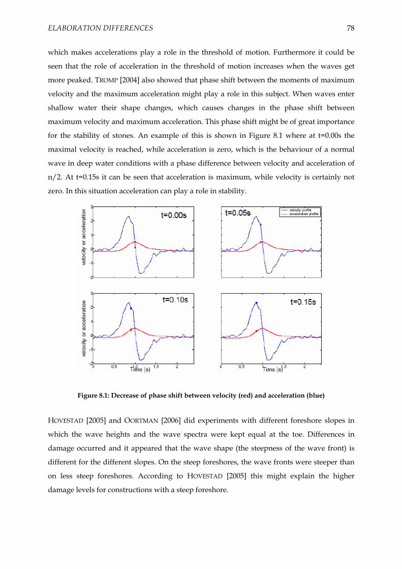
ELABORATION DIFFERENCES 78
which makes accelerations play a role in the threshold of motion. Furthermore it could be
seen that the role of acceleration in the threshold of motion increases when the waves get
more peaked. TROMP [2004] also showed that phase shift between the moments of maximum
velocity and the maximum acceleration might play a role in this subject. When waves enter
shallow water their shape changes, which causes changes in the phase shift between
maximum velocity and maximum acceleration. This phase shift might be of great importance
for the stability of stones. An example of this is shown in Figure 8.1 where at t=0.00s the
maximal velocity is reached, while acceleration is zero, which is the behaviour of a normal
wave in deep water conditions with a phase difference between velocity and acceleration of
π/2. At t=0.15s it can be seen that acceleration is maximum, while velocity is certainly not
zero. In this situation acceleration can play a role in stability.
Figure 8.1: Decrease of phase shift between velocity (red) and acceleration (blue)
HOVESTAD [2005] and OORTMAN [2006] did experiments with different foreshore slopes in
which the wave heights and the wave spectra were kept equal at the toe. Differences in
damage occurred and it appeared that the wave shape (the steepness of the wave front) is
different for the different slopes. On the steep foreshores, the wave fronts were steeper than
on less steep foreshores. According to HOVESTAD [2005] this might explain the higher
damage levels for constructions with a steep foreshore.

ELABORATION DIFFERENCES 79
Structures with a steep foreshore on average show more damage than structures with a less
steep foreshore even if the spectrum at the toe of the structure is identical. In VAN GENT ET
AL. [2003] most of the tests were done with shallow foreshores with two different slope
angles (1:100 and 1:30). In VAN DER MEER [1988] only a limited number of tests (tests 274 to
289) were done with shallow foreshores with a slope angle of 1:30.
To check whether the influence of the foreshore can be seen in the dataset of VAN DER MEER
[1988] in Figure 8.2 and Figure 8.3 the tests with shallow foreshores of VAN DER MEER [1988]
(in red) are plotted together with all data of VAN GENT ET AL. [2003] (in blue). The complete
datasets of VAN DER MEER [1988] and THOMPSON & SHUTTLER [1975] are plotted in grey on
the background. For plunging waves this is done in Figure 8.2. In all graphs maximum
accepted damage levels are applied.
0,0
0,1
0,2
0,3
0,4
0,5
0,6
0,7
0 1 2 3 4 5 6 7 8 9 10
Figure 8.2: Plunging waves: VAN DER MEER [1988] and THOMPSON & SHUTTLER [1975] (grey), VAN DER MEER [1988] with shallow foreshores (red), VAN GENT ET AL. [2003] (blue)
In Figure 8.2 it can be seen the tests with shallow foreshores from the dataset of VAN DER
MEER [1988] do not deviate in an extreme way from of the datasets of VAN DER MEER [1988]
and THOMPSON & SHUTTLER [1975]. However a close look shows that some red data points,
indicated with a red circle, show a bit more damage than the average of the dataset of VAN
DER MEER [1988]. In Figure 8.3 it can be seen that for surging waves the tests with shallow
foreshores of VAN DER MEER [1988] don’t show differences from the rest of the dataset.
γLatham;pl·H2%/∆Dn50 · ξm-1,00,5 · P-0,18 [-]
S/N
0,5 [-
]

ELABORATION DIFFERENCES 80
From this it can be concluded that in the tests of VAN DER MEER [1988] no convincing
influence of shallow foreshores can be seen, because the points that indicate the tests with
shallow foreshores do not show convincing deviations as compared with the rest of the test
results of VAN DER MEER [1988].
0,0
0,1
0,2
0,3
0,4
0,5
0,6
0,7
0,0 0,2 0,4 0,6 0,8 1,0 1,2 1,4 1,6
Figure 8.3: Surging waves: VAN DER MEER [1988] and THOMPSON & SHUTTLER [1975] (grey), VAN DER MEER [1988] with shallow foreshores (red), VAN GENT ET AL. [2003] (blue)
Because in VAN GENT ET AL. [2003] two different slope angles were used for the foreshore it
is also very interesting to check if any differences can be seen in damage for these two slope
angles. Therefore in Figure 8.4 the dataset for plunging waves of VAN GENT ET AL. [2003] is
plotted with the data with cotβ=30 in dark blue and in light blue the data with cotβ=100. The
tests from VAN DER MEER [1988] with shallow foreshores are presented in red. The same is
done for surging waves in Figure 8.5.
In Figure 8.4 it can be seen that for plunging waves in the left part of the graph a certain
distinction appears between the data with cotβ=30 and cotβ=100. The data with cotβ=30
tends to show more damage than the data with cotβ=100. But on the other hand the data
cloud of the data with cotβ=30 is very large for yet unknown reasons. In further research
possible reasons for the large spread in data with cotβ=30 have to be investigated.
γLatham;su·H2%/∆Dn50 · ξm-1,0-P · P0,13 · tanα0,5 [-]
S/N
0,5 [-
]

ELABORATION DIFFERENCES 81
0,0
0,1
0,2
0,3
0,4
0,5
0,6
0,7
0 1 2 3 4 5 6 7 8 9 10
Figure 8.4: Plunging waves: VAN GENT ET Al. [2003] cotβ=30 (dark blue), cotβ=100 (light blue), VAN DER MEER [1988] with cotβ=30 (red)
0,0
0,1
0,2
0,3
0,4
0,5
0,6
0,7
0,0 0,2 0,4 0,6 0,8 1,0 1,2 1,4 1,6
Figure 8.5: Surging waves: VAN GENT ET Al. [2003] cotβ=30 (dark blue), cotβ=100 (light blue), VAN DER MEER [1988] with cotβ=30 (red)
γLatham;pl·H2%/∆Dn50 · ξm-1,00,5 · P-0,18 [-]
S/N
0,5 [-
]
γLatham;su·H2%/∆Dn50 · ξm-1,0-P · P0,13 · tanα0,5 [-]
S/N
0,5 [-
]
ELABORATION DIFFERENCES 82
For surging waves in Figure 8.5 the data with cotβ=30 shows more damage than the data
with cotβ=100 on the whole range. Therefore from Figure 8.5 it can be concluded that for
surging waves the slope of the foreshore has influence on the stability.
In both graphs it can be seen that the tests with shallow foreshores (cotβ=30) from the dataset
of VAN DER MEER [1988] mostly correspond to the data from VAN GENT ET AL. [2003] with
cotβ=100, especially in the graph for surging waves. This would mean, if the model setup is
equal for both datasets, that besides the influence on stability of the foreshore slope angle
also other mechanisms that have not been investigated before might have influence on
stability. A possible mechanism that might have influence on stability is the amount of wave
breaking, which will be discussed in paragraph 8.4. To prove such influences a detailed
analysis of the dataset of VAN GENT ET AL. [2003] is required, which cannot be done in this
M.Sc. Thesis because of the unavailability of this dataset.
Because from the previous section it can be concluded that there is an influence of the
foreshore slope angle on stability a first question that has to be answered is what the
difference is between a foreshore slope and a slope that is a part of the construction. When
for example a slope of 1:8 is schematised as a part of the structure the structure would exist
of 2 different slope angles. VAN DER MEER [1988] did a few tests with an 1:30 foreshore slope
and VAN GENT ET AL. [2003] used an 1:100 and a 1:30 foreshore slope. To recognise a
shallow foreshore we can distinguish 2 conditions (depth and width). According to VAN DER
MOST [1979] a foreshore is shallow when the water depth is sufficiently small (dforeshore/L0 < 1/20). The purpose of a foreshore is to let waves break before they reach the structure, what
will decrease the wave height. When we speak of a shallow foreshore the width of the
sloping foreshore must be at least 2L0 to let wave breaking occur.
To describe the possible influence of a shallow foreshore a connection has to be found
between the shape of the foreshore and stability. The shape of a wave depends on the water
depth and the shape of the foreshore. Entering shallow water the wave steepness increases
and finally the waves will break when the wave steepness reaches critical values.
Accelerations, velocities and phase shift, which obviously affect stability according to
previous sections, depend on the shape of the wave. The wave steepness might be a good
descriptor for this. The shape of a foreshore can be expressed in the water depth and the
slope angle. In this way a possible descriptor for the influence of the foreshore might be a

ELABORATION DIFFERENCES 83
foreshore Iribarren parameter, ξβ, in which the wave steepness and the slope angle of the
foreshore can be combined. A definition for the foreshore Iribarren parameter is given below.
LH %2
tan βξβ =
Where:
β = the foreshore slope angle
H2% = the wave height exceeded by 2% of the waves
L = the wave length (based on Tm-1,0)
To explain the influence of the foreshore Iribarren parameter, ξβ, 4 different model setups
will be distinguished which are presented in Figure 8.6 to Figure 8.9. At first in Figure 8.6
the standard model setup of VAN DER MEER [1988] with deep water at the toe of the
construction and no sloping foreshore can be seen. In this situation cotβ=∞, which makes
ξβ=0.
Figure 8.6: Model setup with deep water at toe and foreshore slope cotβ=∞
Figure 8.7: Model setup with shallow water at toe and foreshore slope cotβ=∞
Figure 8.7 shows a setup with shallow water at the toe of the construction and also no
sloping foreshore. Also in this situation cotβ=∞, which makes ξβ=0. In the latter two model
setups no difference in the foreshore Iribarren parameter can be found. The differences in
damage between these two setups are fully overcome by the use the spectral period, Tm-1,0,
and the wave height exceeded by 2% of the waves, H2%.
H d α
cotβ=∞
H
d L
αcotβ=∞
L

ELABORATION DIFFERENCES 84
Figure 8.8: Model setup with shallow water at toe and foreshore slope cotβ=100
Figure 8.8 shows a situation with shallow water at the toe of the structure and a foreshore
slope of cot β=100 and Figure 8.9 shows a situation with shallow water at the toe of the
construction and a foreshore slope of cot β=30. With equal wave characteristics the value of
ξβ is higher for the situation in Figure 8.9 than for the situation in Figure 8.8. Also according
to the hypothesis that damage increases as the foreshore slope gets steeper, with equal wave
characteristics, the expected damage in the situation in Figure 8.9 will be higher than in the
situation in Figure 8.8. Including a parameter based on ξβ would include the effects on
stability of the foreshore slope angle.
Figure 8.9: Model setup with shallow water at toe and foreshore slope cotβ=30
Because in VAN DER MEER [1988] only 16 tests were done with shallow foreshores no good
reliable regression analysis can be done, but nevertheless the behaviour of a foreshore
Iribarren parameter can be analysed for these 16 tests. Therefore in Table 8.1 values of the
foreshore Iribarren parameter are calculated for all 16 tests with shallow foreshores of VAN
DER MEER [1988].
Because tests with a 1:100 foreshore do not exist in the dataset of VAN DER MEER [1988] in
Table 8.1 four tests have been created with a 1:100 foreshore slope and similar wave
characteristics as the tests with a 1:30 foreshore slope to analyse the influence of the foreshore
slope angle on the foreshore Iribarren parameter and the correction factors. These imaginary
tests are indicated with a star. On the bottom row values of the foreshore Iribarren parameter
are given for the tests of VAN DER MEER [1988] without shallow foreshores. Because the
difference in damage between the datasets of VAN DER MEER [1988] and VAN GENT ET AL.
H
d0
d1
L
α
cotβ=30
H
d0
d1
L
cotβ=100
α

ELABORATION DIFFERENCES 85
[2003] is about 10 to 15% in Table 8.1 it is tried to get a correction factor in a format (1+ ξβn),
with values of 1,1 to 1,15 for 1:30 foreshore slopes. It can be seen that for 1:30 foreshore
slopes this correction factor is higher than for 1:100 foreshore slopes which is in
correspondence with the occurring damage. For situations with cotβ=∞ the correction factor
is 1,0. Of course in a future real regression analysis of these factors more accurate techniques
need to be applied.
Test nr. d
[m]
cotβ
[-]
ξβ
[-]
ξβ2
[-]
(1+ ξβ2)
[-]
ξβ1,5
[-]
(1+ ξβ1,5)
[-]
ξβ1,3
[-]
(1+ ξβ1,3)
[-]
ξβ1,2
[-]
(1+ ξβ1,2)
[-]
274 0,40 30 0,19 0,04 1,04 0,09 1,09 0,11 1,11 0,13 1,13 275 0,40 30 0,23 0,05 1,05 0,11 1,11 0,12 1,12 0,14 1,14 276 0,40 30 0,21 0,04 1,04 0,10 1,10 0,13 1,13 0,15 1,15 277 0,40 30 0,18 0,03 1,03 0,08 1,08 0,15 1,15 0,17 1,17 278 0,40 30 0,24 0,06 1,06 0,12 1,12 0,14 1,14 0,17 1,17 279 0,40 30 0,27 0,07 1,07 0,14 1,14 0,16 1,16 0,18 1,18 280 0,40 30 0,23 0,05 1,05 0,11 1,11 0,16 1,16 0,19 1,19 281 0,40 30 0,25 0,06 1,06 0,12 1,12 0,18 1,18 0,20 1,20 282 0,20 30 0,25 0,06 1,06 0,13 1,13 0,12 1,12 0,15 1,15 283 0,20 30 0,25 0,06 1,06 0,13 1,13 0,12 1,12 0,14 1,14 284 0,20 30 0,25 0,06 1,06 0,12 1,12 0,13 1,13 0,15 1,15 285 0,20 30 0,24 0,06 1,06 0,12 1,12 0,13 1,13 0,15 1,15 286 0,20 30 0,21 0,04 1,04 0,09 1,09 0,16 1,16 0,18 1,18 287 0,20 30 0,20 0,04 1,04 0,09 1,09 0,16 1,16 0,19 1,19 288 0,20 30 0,20 0,04 1,04 0,09 1,09 0,17 1,17 0,19 1,19 289 0,20 30 0,21 0,04 1,04 0,09 1,09 0,17 1,17 0,19 1,19
* 0,40 100 0,07 0,00 1,00 0,01 1,01 0,03 1,03 0,03 1,03 * 0,40 100 0,07 0,00 1,00 0,01 1,01 0,03 1,03 0,03 1,03 * 0,20 100 0,07 0,00 1,00 0,02 1,02 0,03 1,03 0,04 1,04 * 0,20 100 0,07 0,00 1,00 0,02 1,02 0,03 1,03 0,04 1,04
Other 0,80 ∞ 0,00 0,00 1,00 0,00 1,00 0,00 1,00 0,00 1,00
Table 8.1: Behaviour of foreshore Iribarren parameter for tests of VAN DER MEER [1988]
From this the stability formulae of VAN DER MEER [1988] can be changed into the following
formulae:
Plunging waves: ( )5
%218,05,00,1;
50;
11 ⎟⎟⎠
⎞⎜⎜⎝
⎛⋅⋅⋅
Δ⋅⋅⋅+= −
−s
mn
s
plplLath
n
HH
PDH
cNS
αβ ξγξ
Surging waves: ( )5
%25,013,00,1;
50; tan11 ⎟⎟
⎠
⎞⎜⎜⎝
⎛⋅⋅⋅⋅
Δ⋅⋅⋅+= −
−s
Pm
n
s
susuLath
n
HH
PDH
cNS αξγξ αβ

ELABORATION DIFFERENCES 86
Where:
n = factor to be found by regression analysis. Probably n≈1.2to 1.5
In further research to this topic relations between the geometry of the foreshore and the
damage level have to be investigated in which the geometry of the foreshore can be given by
the foreshore Iribarren parameter, ξβ. To prove such relationships if possible damage curves
have to be plotted in which these relations can be shown in a better way. This can be done by
making 3d-curves showing relations between H2%/ΔDn50, ξconstruction, cotα, S/√N and ξforeshore.
By making 3d graphs these curves can be compared with the damage curves of VAN DER
MEER [1988]. An important factor in this is the wave height. A clear definition for the place
where the wave height has to be measured has to be defined. VAN DER MEER [1988] assumed
that the incoming wave height is equal to the wave height at the construction, because in his
investigation no shallow foreshore was present. When a shallow foreshore is present the
wave height at the construction might be affected by processes occurring on the shallow
foreshore, which means that the wave height should be measured at the intersection of mean
water level and the construction. Another possibility is to set up a model to calculate the
wave height at the toe of the construction out of the incoming wave height and the geometry
of the foreshore (BATTJES & GROENENDIJK [2000]).
8.3 Influence of double peaked spectra
In earlier chapters it was already concluded that the wideness of single peaked spectra does
not influence stability. In VAN GENT ET AL. [2003] however also double peaked spectra were
used. To check whether a double peaked spectrum might have a different effect on stability
than a single peaked spectrum in Figure 8.10 from the dataset of VAN GENT ET AL. [2003] for
plunging waves the data with single peaked spectra is compared with the data with double
peaked spectra. In these graphs also a distinction is made between structures with a 1:30 and
1:100 foreshore, because in previous sections it could be concluded that the foreshore slope
angle also influences stability.

ELABORATION DIFFERENCES 87
0,0
0,1
0,2
0,3
0,4
0,5
0,6
0,7
0 1 2 3 4 5 6 7 8 9 10
Van Gent double peakedspectrum cotB=30Van Gent single peakedspectrum cotB=30Van Gent double peakedspectra cotB=100Van Gent single peakedspectra cotB=100
Figure 8.10: Plunging waves: VAN GENT ET AL. [2003] Single peaked spectra, double peaked spectra
0,0
0,1
0,2
0,3
0,4
0,5
0,6
0,7
0,0 0,2 0,4 0,6 0,8 1,0 1,2 1,4 1,6
Van Gent double peakedspectra cotB=30Van Gent single peakedspectra cotB=30Van Gent double peakedspectra cotB=100Van Gent single peakedspectra cotB=100
Figure 8.11: Surging waves: VAN GENT ET AL. [2003] Single peaked spectra), double peaked spectra
In Figure 8.10 in general a distinction appears between the data with single peaked and
double peaked spectra. It can be seen that the data with single peaked spectra and cotβ=30
γLatham;pl·H2%/∆Dn50 · ξm-1,00,5 · P-0,18 [-]
S/N
0,5 [-
]
γLatham;su·H2%/∆Dn50 · ξm-1,0-P · P0,13 · tanα0,5 [-]
S/N
0,5 [-
]

ELABORATION DIFFERENCES 88
on average show more damage than the data with double peaked spectra and cotβ=30, but
this may also be caused by the absence of data with double peaked spectra on the left part of
the graph. Also there is a lot of scatter in both data clouds. For cotβ=100 there is no clear
distinction between single and double peaked spectra. To be able to make a proper
conclusion from this more research on this topic is required.
In Figure 8.11 the same graph is given for surging waves. In this graph no clear distinction
can be seen between data with double peaked and single peaked spectra.
8.4 Wave breaking
In Figure 8.12 the test results for plunging waves of VAN GENT ET AL. [2003] have been
plotted again. A distinction has been made in the amount of wave breaking. Severe wave
breaking occurs for Hs;toe / Hs;deep <0,7, intermediate wave breaking occurs for 0,7 < Hs;toe /
Hs;deep <0,9 and only a small amount of wave breaking occurs for Hs;toe / Hs;deep > 0,9. In this
figure no clear relation can be seen between the amount of wave breaking on the foreshore
and the damage level.
Figure 8.12: Plunging waves VAN GENT ET AL. [2003] with distinction in amount of wave breaking

ELABORATION DIFFERENCES 89
In future research to this topic more research has to be done to the wave height distribution
on the foreshore in the tests of VAN GENT ET AL. [2003] and the effects on stability of the
wave breaking processes on the foreshore. This also includes a test whether the wave height
relations from BATTJES & GROENENDIJK [2000] are valid for the data of VAN GENT ET AL.
[2003].
Because in shallow waters the wave height strongly depends on the water depth for the data
of VAN GENT ET AL. [2003] the damage level may also directly be influenced by the water
depth instead of the wave height. Also because of difficulties in measuring wave heights of
breaking waves it might be better to use the water depth in shallow water conditions, which
forms a more fixed value. Therefore in future research to this topic also possible relations
between the water depth and the damage level in shallow water conditions have to be
investigated.
8.5 Surf beat and wave reflection
Surf beat occurs when deep water waves propagate into shallow water. Entering shallow
water they exhibit increasingly strong nonlinearities. One important nonlinear effect is the
emergence of low-frequency energy as a consequence of interactions between higher
frequency incident wave components. The low-frequency components with periods of
several minutes cause water level variations in the surf zone. Compared with wave impact
on average surf beat has only a minor contribution to the forces acting on the stones and
therefore it is in most situations neglectable. However when wave heights are low (in the
order of centimetres), the effects of surf beat on stability may not be neglectable. The same
can be said for the effects of wave reflection. In model tests of VAN DER MEER [1988] and
THOMPSON & SHUTTLER [1988] the wave height varies between 0,02m and 0,26m for the small
scale tests, which indicates that surf beat and wave reflection may have affected the stability
of stones during these tests, especially for the lower wave heights.
In Figure 8.13 the datasets of VAN DER MEER [1988] and THOMPSON & SHUTTLER [1975] have
been plotted. In these graphs a distinction is made between Hs<0,10m (blue) and Hs>0,10m
(red). In these graphs it can be seen that the data with Hs<0,10m does not show different
damage patterns than the data with Hs>0,10m. Also it can be seen that the amount of scatter
is about equal for both groups of data. From this it can be concluded that for the datasets of

ELABORATION DIFFERENCES 90
0,0
0,1
0,2
0,3
0,4
0,5
0,6
0,7
0,0 0,2 0,4 0,6 0,8 1,0 1,2 1,4 1,6
0,0
0,1
0,2
0,3
0,4
0,5
0,6
0,7
0 1 2 3 4 5 6 7 8 9 10
VAN DER MEER [1988] and THOMPSON & SHUTTLER [1975] the influence of small scale effects
like surf beat and wave reflection can not be visualized by making a distinction between
smaller and larger significant wave heights. However this does not mean that these small
scale effects do not influence stability.
Figure 8.13: Plunging waves (left) and surging waves (right) of VAN DER MEER [1988] and THOMPSON & SHUTTLER with distinction in Hs<0,10m (blue) and Hs>0,10m (red)
γLatham;su·H2%/∆Dn50 · ξm-1,0-P · P0,13 · tanα0,5 [-]
S/N
0,5 [-
]
γLatham;pl·H2%/∆Dn50 · ξm-1,00,5 · P-0,18 [-]
S/N
0,5 [-
]

91
Chapter 9 CONCLUSIONS AND RECOMMENDATIONS
CONCLUSIONS &
RECOMMENDATIONS
9.1 General conclusion
The main conclusion from this report is that the foreshore slope angle influences stability in
the dataset of VAN GENT ET AL. [2003]. After transforming the datasets of THOMPSON &
SHUTTLER [1975] and VAN DER MEER [1988] into comparable datasets with the dataset of VAN
GENT ET AL. [2003] still differences can be seen between the datasets of VAN DER MEER [1988]
/ THOMPSON & SHUTTLER [1975] and the dataset of VAN GENT ET AL. [2003]. These
differences are visible in the reconstructed graphs and have been statistically confirmed by
using the T-test. In this for all 3 datasets the wave height was expressed in the wave height
exceeded by 2% of the waves, H2%, and the wave period was expressed in the spectral wave
height, Tm-1,0. Transformation of the original datasets of VAN DER MEER [1988] and
THOMPSON & SHUTTLER [1975], in which for the wave height the significant wave height, Hs,
was used and for the wave period the mean wave period, Tm, was used, was done on a
individual basis. This means no generally applicable ratios where used which were used for
the comparison in VAN GENT [2004]. Besides the correct transformation of wave height and

CONCLUSIONS & RECOMMENDATIONS 92
wave period also the influences of stone roundness, which caused some deviations in the
original dataset of VAN DER MEER [1988], and maximum acceptable damage levels were
incorporated in this M.Sc. Thesis.
In the final graphs it can be seen that on average the data of VAN GENT ET AL. [2003] still
shows more damage than the data of VAN DER MEER [1988] and THOMPSON & SHUTTLER
[1975]. The datasets of VAN DER MEER [1988] and THOMPSON & SHUTTLER [1975] do not show
significant differences. An explanation for these differences can be found in the fact that most
of the tests of VAN GENT ET AL. [2003] were tests with shallow water conditions (shallow
foreshores), while the majority of the tests of VAN DER MEER [1988] and THOMPSON &
SHUTTLER [1975] were done in deep water conditions. Experiments of a number of M.Sc.
students at Delft University of Technology indicated that wave deformation on shallow
foreshores causes different damage patterns as compared with standard waves. On average
constructions with steep foreshores show more damage than constructions with less steep
foreshores. This was also visible in the data of VAN GENT ET AL. [2003]. The influence of
acceleration and the phase shift between velocity and acceleration may also play an
important role in this (VERHAGEN [2005]).
9.2 Recommendations
To get a better understanding of the differences between the datasets more research to this
topic is required. However a possible explanation can be the influence of acceleration and
phase shift because of wave deformation, other possible differences between the experiments
must also be taken into account. In this M.Sc. Thesis it already became clear that stone
roundness had a quite spectacular influence on stability, but it might just as well be possible
that many other at present unknown factors play a role on stability too.
Further research to this topic requires the availability and accessibility of the dataset of VAN
GENT ET AL. [2003]. A first thing to be done would be to check if in the dataset of VAN GENT
ET AL. [2003] itself also a distinction occurs between tests results with deep water conditions
and shallow water conditions. The inclusion of a new factor, based on the foreshore Iribarren
parameter as described in paragraph 8.2, in the modified formulae of VAN DER MEER [1988]
should lead to a decrease of the differences between the datasets of VAN DER MEER [1988] /
THOMPSON & SHUTTLER [1975] and VAN GENT ET AL. [2003].

93
REFERENCES
BATTJES, J.A., & GROENENDIJK, H.W. [2000]
Wave height distribution on shallow foreshores
Coastal engineering 40, Elsevier
DESSENS, M. [2004]
The influence of flow acceleration on stone stability
M.Sc. Thesis, Delft University of Technology
GENT, M.R.A. VAN, SMALE, A., KUIPER, C. [2003]
Stability of rock slopes with shallow foreshores
Proc. Coastal structures 2003, Portland, ASCE
GENT, M.R.A. VAN [2004]
On the stability of rock slopes
Keynote NATO Workshop May 2004 Bulgaria
Goda, Y. [1988]
On the Methodology of Selecting Design Wave Height
Coastal engineering 1988
A review on statistical interpretation of wave data.
Report of the Port and Harbour Research Institute, Japan
HOVESTAD, M. [2005]
Breakwaters on steep foreshores
M.Sc. Thesis, Delft University of Technology
INFRAM report i 489 [2001]
Verhouding piekperiode en spectrale periodemaat
LATHAM, J.-P., MANNION, M.B., POOLE, A.B. BRADBURY A.P. AND ALLSOP, N.W.H. [1988]
The influence of armour stone shape and rounding on the stability of breakwater armour
layers.
Queen Mary College, University of London, UK

REFERENCES 94
LONGUET-HIGGINS, M.S. [1980]
On the distribution of the heights of sea waves: some effects of nonlinearity and finite band
width
J. Geophys.
MEER, J.W. VAN DER [1988]
Rock slopes and gravel beaches under wave attack
Ph.D. Thesis, WL | Delft Hydraulics (report 396) and Delft University of Technology
OORTMAN, N.J. [2006]
Influence of foreshore steepness on wave velocity and acceleration at the breakwater
interface.
M.Sc. Thesis, Delft University of Technology
TERILLE, E. [2004]
The threshold of motion of coarse sediment particles by regular non-breaking waves
M.Sc. Thesis, Delft University of Technology, University of Genoa
TERILLE, E. [2004]
Incipient motion of coarse particles under regular shoaling waves
Coastal Engineering December 2004
THOMPSON, D.M., SHUTTLER, R.M. [1975]
Riprap design for wind wave attack. A laboratory study in random waves
Wallingford, EX 707
TROMP, M. [2004]
Influences of fluid accelerations on the threshold of motion
M.Sc. Thesis, Delft University of Technology
VERHAGEN, H.J. [2005]
The effect of foreshore slope on breakwater stability
ASCE, Proc. ICCE 2005
WL | DELFT HYDRAULICS, M1983 DEEL I [1988]
Statistische stabiliteit van stortsteentaluds onder golfaanval. Ontwerp formules.
Verslag modelonderzoek, M1983 deel I

95
APPENDIX A THEORY
A1 Wave height distribution on shallow foreshores
The conversion from Hs to H2% can be done using the point model of BATTJES & GROENENDIJK
[2000]. The point model of BATTJES & GROENENDIJK [2000] describes the wave height
distribution on a shallow foreshore. This model consists of a Rayleigh distribution, or a
Weibull distribution with the exponent equal to 2, for the lower wave heights and a Weibull
distribution with a higher exponent for the higher wave heights. This composite Weibull
distributed is shown in Figure A.1.
Figure A.1: Probability density function (BATTJES & GROENENDIJK [2000])
The theoretical expression of the composite Weibull distribution is shown below.
( ) { }( )
( ) tr
tr
k
k
HH
HH
HHHF
HHHF
HHHF≥
≤
⎪⎪⎪
⎩
⎪⎪⎪
⎨
⎧
⎥⎥⎦
⎤
⎢⎢⎣
⎡⎟⎟⎠
⎞⎜⎜⎝
⎛−−=
⎥⎥⎦
⎤
⎢⎢⎣
⎡⎟⎟⎠
⎞⎜⎜⎝
⎛−−=
=≤≡2
1
22
11
exp1
exp1
Pr
Rayleigh
Weibull

APPENDIX A1 96
In which:
k1, k2 = shape parameters of the distribution determining the curvature
H1, H2 = scale parameters
Htr = transition wave height: Htr = ⎟⎟⎠
⎞⎜⎜⎝
⎛⋅⋅⋅=
cctrtr L
dLH πβ 2tanh14,0
Where:
βtr = slope-dependent coefficient: αβ tan43 cctr += ; (c3 = 0,46, c4 = 9,25)
Lc = characteristic local wave height defined by: ⎟⎟⎠
⎞⎜⎜⎝
⎛⋅=
c
cc L
dgTL π
π2tanh
2
2
The introduction of the wave period in the expression for Htr gave insignificant
improvements comparing with the point model using a transitional wave height depending
on the bottom slope and depth only. Therefore a simpler parameterisation for the transitional
wave height is given by:
( ) dH tr ⋅⋅+= αtan8,535,0
For the shape parameters k1 and k2 BATTJES & GROENENDIJK [2000] uses k1 = 2 and k2 = 3,6.
For the root mean square wave height the root mean square of the sampled zero-crossing
wave height per record is used. Using the deep-water ratio of 0mH rms for broad banded
sea as a constraint for the root mean square wave height is found:
( ) 00
0 24,369,269,2 mdm
mH rmsrms ⎟⎟⎠
⎞⎜⎜⎝
⎛⋅+=⋅+= ψβ
The only unknown parameters in the model described above are the scale parameters H1 and
H2. These can be calculated by solving the following expression in terms of the incomplete
gamma functions γ(a,x) and Г(a,x) (ABRAMOWITZ & STEGUN [1964]). This gives:
1~~
,12~~~
,12~~21
22
22
11
21 =
⎥⎥⎦
⎤
⎢⎢⎣
⎡⎟⎟⎠
⎞⎜⎜⎝
⎛+Γ⋅+
⎥⎥⎦
⎤
⎢⎢⎣
⎡⎟⎟⎠
⎞⎜⎜⎝
⎛+⋅=
k
tr
k
trrms H
Hk
HHH
kHH γ
resulting in:

APPENDIX A1 97
( ) ( ) 1exp~exp~~6,3
2
95
2
1
~~
22
~~
0
21 =⋅−⋅⋅+⋅−⋅⋅= ∫∫
∞
⎟⎟⎠
⎞⎜⎜⎝
⎛
⎟⎟⎠
⎞⎜⎜⎝
⎛
HH
HH
rms
tr
tr
dtttHdtttHH
where :
6,3
2
2
1~~
~~
⎟⎟⎠
⎞⎜⎜⎝
⎛=⎟⎟
⎠
⎞⎜⎜⎝
⎛HH
HH trtr
In order to make this calculation a lot easier BATTJES & GROENENDIJK [2000] set up a table
with the characteristic normalised wave heights as a function of the transitional wave height.
To use this table the normalised transitional wave height is needed. This parameter is
expressed by:
rms
trtr H
HH =~
Corresponding to each value of the normalised transitional wave height in Table A.1 values
of several normalised characteristic wave heights are given in the table. The table from
BATTJES & GROENENDIJK [2000] is given on the next page for H2% and H1/3. With these values
the ratio H2%/H1/3 is calculated.

APPENDIX A1 98
Htr H2% H1/3 H2%/H1/3 0,00 1,548 1,279 1,210 0,05 1,548 1,279 1,210 0,10 1,548 1,279 1,210 0,15 1,548 1,279 1,210 0,20 1,548 1,279 1,210 0,25 1,548 1,279 1,210 0,30 1,548 1,279 1,210 0,35 1,548 1,279 1,210 0,40 1,548 1,279 1,210 0,45 1,549 1,279 1,211 0,50 1,549 1,280 1,210 0,55 1,550 1,281 1,210 0,60 1,552 1,282 1,211 0,65 1,554 1,284 1,210 0,70 1,557 1,286 1,211 0,75 1,561 1,290 1,210 0,80 1,567 1,294 1,211 0,85 1,573 1,300 1,210 0,90 1,582 1,307 1,210 0,95 1,591 1,315 1,210 1,00 1,603 1,324 1,211 1,05 1,616 1,335 1,210 1,10 1,630 1,346 1,211 1,15 1,645 1,359 1,210 1,20 1,662 1,371 1,212 1,25 1,679 1,381 1,216 1,30 1,698 1,389 1,222 1,35 1,717 1,395 1,231 1,40 1,737 1,399 1,242 1,45 1,757 1,403 1,252
Htr H2% H1/3 H2%/H1/3 1,50 1,778 1,406 1,265 1,55 1,799 1,408 1,278 1,60 1,820 1,410 1,291 1,65 1,841 1,411 1,305 1,70 1,863 1,412 1,319 1,75 1,884 1,413 1,333 1,80 1,906 1,413 1,349 1,85 1,927 1,414 1,363 1,90 1,949 1,414 1,378 1,95 1,970 1,415 1,392 2,00 1,985 1,415 1,403 2,05 1,983 1,415 1,401 2,10 1,982 1,415 1,401 2,15 1,981 1,415 1,400 2,20 1,981 1,415 1,400 2,25 1,980 1,415 1,399 2,30 1,979 1,415 1,399 2,35 1,979 1,415 1,399 2,40 1,979 1,416 1,398 2,45 1,979 1,416 1,398 2,50 1,978 1,416 1,397 2,55 1,978 1,416 1,397 2,60 1,978 1,416 1,397 2,65 1,978 1,416 1,397 2,70 1,978 1,416 1,397 2,75 1,978 1,416 1,397 2,80 1,978 1,416 1,397 2,85 1,978 1,416 1,397 2,90 1,978 1,416 1,397 2,95 1,978 1,416 1,397 3,00 1,978 1,416 1,397
Table A.1: table from Battjes & Groenendijk [2000] for H2% and H1/3

99
A2 Wave spectra
Ocean waves can be described by a wave spectrum. The aim of describing waves with a
wave spectrum is not to describe one observation of the sea surface in detail. In a wave
spectrum the sea surface is described as a stochastic process, which means that all possible
observations that could have been made are characterised.
The surface elevation in a time record, η(t), with a duration D is a very chaotic process which
can exactly be reproduced as the sum of a large number of harmonic wave components (a
Fourier series):
( ) ( )∑=
+=N
iiii tfat
1
2cos απη
Each wave component has it’s own amplitude (a), phase difference (α) and frequency (f). The
next step in order to create a wave spectrum is to make an amplitude spectrum. To do this
for each frequency interval (Δf=1/D) the corresponding amplitude is plotted. In another
observation other values of the corresponding amplitudes will be found, but by repeating the
experiment many times (M) and take the average over all experiments the average amplitude
spectrum can be found. From this the amplitude density ( fai Δ/ ) can be calculated for each
frequency.
A more meaningful way to describe the waves would be to calculate the variance density
( fai Δ/22
1 ) of each frequency step, because of two reasons:
• the variance is a more relevant statistical quantity than the amplitude;
• the variance is proportional to the wave energy.
By letting the frequency interval approach to zero (Δf → 0) a continuous distribution of the
variance density can be made. The variance density spectrum can now be described as:
( ) { }22
10
1lim ii
faE
ffE
Δ=
→Δ

APPENDIX A2 100
By multiplying the variance density spectrum with ρg the energy density spectrum is
obtained.
A lot of research has been done to the shape of the wave spectrum. Observations by PIERSON
AND MOSKOWITZ [1964] in an assumed fully sea state in deep water resulted in a f-5 –shape
for higher frequencies. The Pierson-Moskowitz spectrum is given by the following equation:
( ) ( )⎪⎭
⎪⎬⎫
⎪⎩
⎪⎨⎧
⎟⎟⎠
⎞⎜⎜⎝
⎛−⋅⋅⋅⋅=
−
−−4
542
45exp2
PMPMPM f
ffgfE πα
The shape of the wave spectrum depends on the overall appearance of the waves. The
narrower the spectrum is, the more regular the waves are. The narrowest spectrum describes
a wave record of a harmonic wave. This spectrum is a delta function (spike) at one
frequency. The wider the spectrum gets, the more chaotic the wave record is.
Because fully developed sea states do not often occur in reality and observations have shown
that in fetch-limited conditions the spectra show a sharper and higher peak than in fully
developed conditions. Because of this scientists of JONSWAP (Joint North Sea Wave Project)
chose to use the shape of the Pierson-Moskowitz spectrum and enhance its peak with a peak
enhancement function. This resulted in:
( ) ( )⎥⎥⎥⎥
⎦
⎤
⎢⎢⎢⎢
⎣
⎡
⎟⎟⎟⎟
⎠
⎞
⎜⎜⎜⎜
⎝
⎛ −−
−
−− ⋅⎪⎭
⎪⎬⎫
⎪⎩
⎪⎨⎧
⎟⎟⎠
⎞⎜⎜⎝
⎛−⋅⋅⋅⋅=
21
21exp
4542
45exp2
σ
γπα
peakff
PMPMJONSWAP f
ffgfE
For example in Figure A.2 the Pierson-Moskowitz–spectrum, PM-spectrum, is plotted
together with the JONSWAP-spectrum with equal wave conditions.

APPENDIX A2 101
0,000
0,005
0,010
0,015
0,020
0,025
0,030
0,035
0,040
0,045
0,050
0 0,2 0,4 0,6 0,8 1 1,2
f
E(f)
PM
Jonsw ap
Figure A.2: PM- spectrum and JONSWAP-spectrum

102
A3 Ratio peak period to spectral period
In INFRAM I489 [2001] the ratio peak period to spectral period has been calculated for various
tests. Also for a number of tests from DELFT HYDRAULICS, M1983 PART I [1988] this ratio was
investigated. In this paper different definitions for the peak period and the spectral period
are given:
Tp The frequency at which the energy in the energy density spectrum is at it’s
maximum. The peak period is the inverse of the peak frequency (Tp = 1/fp). A
disadvantage is that this value depends on the ‘smoothness’ of the spectrum.
Tp;a The peak period using a cut off frequency for the higher frequencies.
Tp;b The peak period from the part of the spectrum for which the energy is more than 40%
of the maximum value. This value gives a more fixed value than the Tp as described
before. This value was calculated over the whole frequency range.
Tp;d The peak period from the part of the spectrum for which the energy is more than 80%
of the maximum value. This value was calculated over the whole frequency range.
Tm-1,0 The spectral period Tm-1,0 = m-1/m0, in which m-1 and m0 are respectively the first
negative and the zero-th order moment of the spectrum calculated over the whole
frequency range.
Tm-1,0;a The spectral period Tm-1,0 = m-1/m0, in which m-1 and m0 are respectively the first
negative and the zero-th order moment of the spectrum using a cut-off frequency for
the lower frequencies.
To make this clear in Figure A.3 an example of a spectrum is given. In this figure the cut off
frequency is shown and also the meaning of the 40%- and 80% energy value used in Tpb and
Tpd is shown.

APPENDIX A3 103
Figure A.3: Wave spectrum with cut-of frequency and 40%- and 80% energy value
In INFRAM I489 [2001] the analysed spectra are digitalised. From these digitalised spectra the
peak period, Tp, and the spectral period,Tm-1,0, are obtained. The results of this are given in
Table A.2.
For test 25 the spectral period, Tm-1,0, has been recalculated in this M.Sc. Thesis. The spectral
period, Tm-1,0 can be calculated using the following expression:
( )
( )
( )
( )∫
∫
∫
∫∞
∞−
∞
∞−
−− ===
0
0
1
0
0
0
1
0
10,1
dffE
dffEf
dffEf
dffEf
mm
Tm
In order to calculate the spectral period the wave spectrum from test 25 first has to be
digitalised. This has been done with a step size of 0,02. After this the surface of each step has
been calculated where after the spectral moments, m-1 and m0, can be calculated by
calculating the surface under the spectral curve. For test 25 this resulted in a calculated
spectral moment, Tm-1,0, of:
0,000
0,005
0,010
0,015
0,020
0,025
0,030
0,035
0,040
0,045
0,050
0 0,2 0,4 0,6 0,8 1 1,2f
E(f)
80% value (for Tpd)
40% value (for Tpb)
Cut off frequency

APPENDIX A3 104
sTm 502,21683,04210,0
0,1 ==−
and: sT am 425,21669,04047,0
;0,1 ==−
These calculated values are very close to the values calculated in INFRAM I489 [2001], where
Tm-1,0 = 2,491s and Tm-1,0;a = 2,413s. The small differences can be explained because of the
better accuracy in the calculations of INFRAM I489 [2001].
Data from DELFT HYDRAULICS, M1983 PART I [1988]
Calculated with a digitalised spectrum
testnr. Tp [s]
Hs
[m]) Spectrum Cut off
freq. [Hz] Tp [s]
Tm-1,0 [s]
Tm-1,0a [s]
Tpb [s]
Tp/Tm-1,0 [-]
Tpb/Tm-1,0a [-]
26 3,17 0,117 I 0,2 3,092 3,079 2,887 3,093 1,00 1,07
60 2,17 0,116 I 0,2 1,999 2,153 2,032 2,110 0,93 1,04
21 2,53 0,118 I 0,2 2,664 2,559 2,384 2,471 1,04 1,04
24 2,53 0,109 I 0,2 2,679 2,52 2,372 2,440 1,06 1,03
22 2,56 0,100 I 0,2 2,697 2,561 2,422 2,518 1,05 1,04
23 2,53 0,086 I 0,2 2,687 2,497 2,393 2,503 1,08 1,05
25 2,53 0,071 I 0,2 2,625 2,491 2,413 2,492 1,05 1,03
186 3,23 0,097 II 0,2 3,200 3,244 3,171 3,187 0,99 1,01
161 2,24 0,111 II 0,2 2,220 2,511 2,271 2,244 0,88 0,99
164 1,79 0,119 II 0,2 1,788 1,953 1,819 1,801 0,92 0,99
195 1,40 0,124 II 0,2 1,384 1,462 1,462 1,399 0,95 0,96
175 4,25 0,106 III 0,05 4,354 3,854 3,788 4,076 1,13 1,08
182 3,17 0,112 III 0,05 3,032 2,813 2,813 2,884 1,08 1,03
171 2,67 0,122 III 0,05 2,715 2,357 2,316 2,513 1,15 1,09
188 1,83 0,125 III 0,05 1,701 1,672 1,672 1,768 1,02 1,06
Table A.2: Ratios Tp / Tm-1,0 for tests from DELFT HYDRAULICS, M1983 PART I [1988]
From this table the average Tp/Tm-1,0 ratios can be calculated for the different spectral shapes.
This is done in Table A.3 where also the standard deviations are given. In this table also the

APPENDIX A3 105
ratio Tpb/Tm-1,0a was calculated which shows a smaller standard deviation than the
ratio Tp/Tm-1,0, and thus forms a better fixed value.
Tpb/Tm-1,0a Standard
Deviation
Tp/Tm-1,0 Standard
Deviation
Spectrum I 1,042 0,013 1,031 0,047
Spectrum II 0,985 0,018 0,933 0,038
Spectrum III 1,061 0,023 1,094 0,052
Table A.3: Average ratios peak period / spectral period and standard deviations
According to INFRAM I489 [2001] the ratios Tp/Tm-1,0 of the tests from DELFT HYDRAULICS,
M1983 PART I [1988] are smaller than the average value from the other tests. The report
recommends a fixed ratio Tp/Tm-1,0 of 1,1. In earlier research it was found that for JONSWAP-
spectra this ratio would be 1,11 and for a wider PM-spectrum the ratio would increase to
1,17. For the tests from DELFT HYDRAULICS, M1983 PART I [1988] the report recommends a
fixed value of 1,04, instead of 1,1. This difference can be explained when a close look is given
to the spectra used in DELFT HYDRAULICS, M1983 PART I [1988]. Therefore in Appendix B the
spectra from DELFT HYDRAULICS, M1983 PART I [1988] have been plotted with a real PM-
spectrum on the background in red. In Appendix B it can be seen that the spectra from the
tests with PM-spectra are significantly narrower on the right tail than the original PM-
spectra. This can explain why the peak period, Tp, and the spectral period,Tm-1,0, converge.

106
A4 The T-Test
To check whether the means of two datasets, or parts of datasets are statistically different
from each other the T-test can be used. The T-test is especially appropriate for posttest
analysis of two different groups of randomized experiments. This makes the T-test very
applicable on the subject of this M.Sc. Thesis.
Figure A.4: Idealized distributions for treated and comparison group posttest values
In Figure A.4 the distributions for the group 1 (red) and group 2 (blue) groups in a study are
shown. It must be mentioned that the figure shows an idealized distribution, because the
actual distribution would usually be a histogram. In Figure A.4 it can be seen where the
control and treatment group means are located. The T-test can address whether the means
are statistically different or not.
In Figure A.5 examples are given of samples with the same mean, but different variations. In
this figure cases with medium, high and low variability are shown. Two groups are most
statistically different in the bottom or low-variability case, because there is relatively little
overlap between the two bell-shaped curves. In the high variability case, the group
difference least, because the two bell-shaped distributions overlap very much.
Group 1 Group 2

APPENDIX A4 107
Figure A.5: Three scenarios for differences between means
From this it can be concluded that differences between scores for two groups can be judged
by analysing the difference between their means relative to the spread or variability of their
scores.
The T-test to determine whether two groups, X and Y, are statistically different is shown
below. At first the value of tobs has to be calculated.
Y
Y
X
X
obs
ns
ns
YXgroupsofiability
meansgroupbetweendifferencet22var
+
−==
Where:
X = group mean of group X (x1, x2, ……..xn)
Y = group mean of group Y (y1, y2, ……..yn)
sX, sY = standard deviation of group X or group Y
nX, nY = number of tests of group X or group Y
A positive value of tobs indicates that the mean of group X is larger than the mean of group Y
and a negative value of tobs indicates that the mean of group X is lower than the mean of
group Y. Once the value of tobs is determined the risk level (or alpha level) has to be set. In
Medium variability
Low variability
High variability

APPENDIX A4 108
most social research, the "rule of thumb" is to set the alpha level at 0.05. This means that five
times out of a hundred a statistically significant difference exists between the means even if
there was none.
After this the degrees of freedom (dof) for the test need to be determined. In the T-test, the
degrees of freedom is the sum of the experiments in both groups minus 2. Given the alpha
level, the dof, and the tobs-value, the t-value has to be looked up in a standard table of
significance to determine whether the t-value is large enough to be significant. If it is it can
be concluded that the two groups are statistically different.

109
APPENDIX B SPECTRA VAN DER MEER [1988]
Tests with PM-spectra:
Test 25
0
5
0
5
Test 23 Test 22
Test 24 Test 21 Test 60
Test 26

APPENDIX B 110
Tests with narrow spectra:
Test 164
0
Test 195 Test 161
Test 186

APPENDIX B 111
Tests with wide spectra:
00
05
0
5
Test 171
00
Test 188 Test 182
Test 175

112
APPENDIX C STONES VAN DER MEER [1988]
Riprap after 134 tests, 2x painted

APPENDIX C 113
Uniform stone after 106 tests, 1x painted
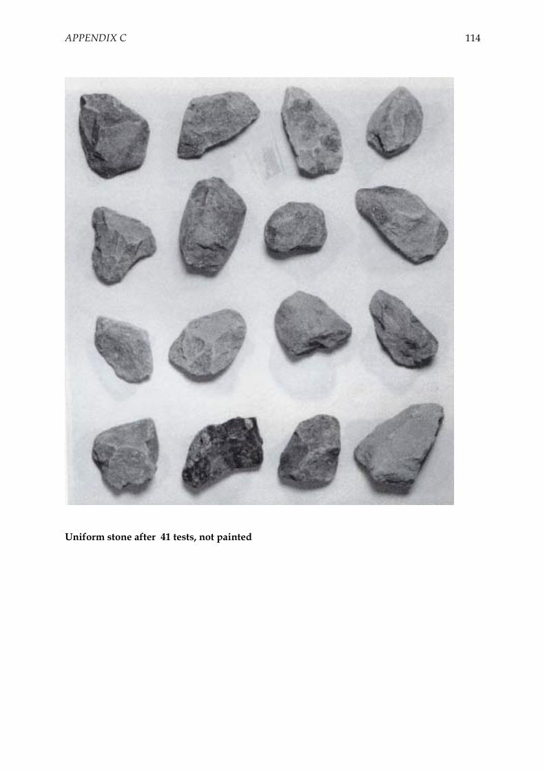
APPENDIX C 114
Uniform stone after 41 tests, not painted
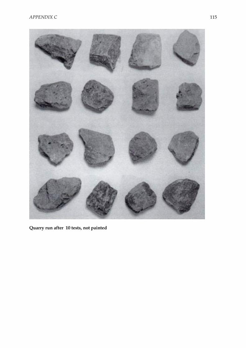
APPENDIX C 115
Quarry run after 10 tests, not painted

APPENDIX C 116
Basalt after 10 tests, not painted

117
APPENDIX D LEGEND GRAPHS VAN DER MEER
Impermeable cota=3 ; N=3000
Impermeable cota=4 ; N=3000
Impermeable cota=6 ; N=3000
Spectrum Narrow ; N=3000
Spectrum Wide ; N=3000
Permeable cota=3 ; N=3000
Permeable cota=2 ; N=3000
Permeable cota=1,5 ; N=3000
Homogenous ; N=3000
Depth 0,4m ; N=3000
Depth 0,2m ; N=3000
Delta 0,92 ; N=3000
Delta 2,05 ; N=3000
Large scale ; N=3000
Impermeable cota=3 ; N=1000
Impermeable cota=4 ; N=1000
Impermeable cota=6 ; N=1000
Spectrum Narrow ; N=1000
Spectrum Wide ; N=1000
Permeable cota=3 ; N=1000
Permeable cota=2 ; N=1000
Permeable cota=1,5 ; N=1000
Homogenous N=1000
Depth 0,4m ; N=1000
Depth 0,2m ; N=1000
Delta 0,92 ; N=1000
Delta 2,05 ; N=1000
Large scale ; N=1000

118
APPENDIX E DETAILED GRAPHS
0,0
0,1
0,2
0,3
0,4
0,5
0,6
0,7
0 1 2 3 4 5 6 7 8 9 10
FigureA.6: Plunging waves with maximum accepted damage levels: THOMPSON & SHUTTLER [1975] (green), VAN DER MEER [1988] (red), VAN GENT ET AL. [2003] (blue)

APPENDIX E 119
0,0
0,1
0,2
0,3
0,4
0,5
0,6
0,7
0,0 0,1 0,2 0,3 0,4 0,5 0,6 0,7 0,8 0,9 1,0 1,1 1,2 1,3
FigureA.7: Surging waves with maximum accepted damage levels: THOMPSON & SHUTTLER [1975] (green), VAN DER MEER [1988] (red), VAN GENT ET AL. [2003] (blue)