comparison of automotive structures using transmissibility ...comparison of automotive structures...
TRANSCRIPT

Comparison of Automotive Structures Using Transmissibility Functions and Principal
Component Analysis
A thesis submitted to the
Division of Research and Advanced Studies
of the University of Cincinnati
in partial fulfillment of the
requirements for the degree of
MASTER OF SCIENCE
School of Dynamic Systems, Mechanical Engineering Program
College of Engineering and Applied Science
March 31, 2013
by
Matthew Randall Allemang
Bachelor of Science in Mechanical Engineering
University of Cincinnati, Cincinnati, Ohio, USA, 2005.
Thesis Advisor and Committee Chair: Dr. Robert Rost
Committee Members: Dr. David L. Brown, Dr. Allyn Phillips

ii
Abstract
The focus of this thesis is developing alternate methods for comparing various fully
trimmed vehicle body structures. Traditionally, experimental modal analysis has been used to
achieve this, but has seen limited success. The challenge is developing global trends using
information from very distinct points. This thesis examines the use of single input and multi-
input transmissibility as measured on a four post road simulator as an alternate means to compare
similar or dissimilar vehicle structures.
Early work with transmissibility indicated some differences in vehicle structures, but
suffered from some of the same problems as experimental modal analysis techniques. A group
transmissibility concept was developed in a parallel thesis[1], but the most promising work
focused on use of principal component analysis (PCA) to reduce large amounts of data to a
smaller set of representative data. Principal Component Analysis (PCA) methods have been
variously developed and applied within the experimental modal and structural dynamics
community for some time. While historically the use of these techniques has been restricted to
the areas of model order determination utilizing the complex mode indicator function (CMIF),
enhanced frequency response function (eFRF) and virtual response function estimation, and
parameter identification, increasingly the PCA methodology is being applied to the areas of
test/model validation, experimental model correlation/repeatability and experimental/structural
model comparison. With the increasing volume of data being collected today, techniques which
provide effective extraction of the significant data features for quick, easy comparison are
essential. This thesis also explores the general development and application of PCA to
transmissibility measurements and the ability of PCA to provide the analyst with an effective
global trend visualization tool.

iii

Acknowledgements
First, I would like to thank my committee members, Dr. Bob Rost, Dr. Dave Brown, and
Dr. Allyn Phillips for their input and support both on this thesis and throughout my academic
career.
I would like to thank my project colleagues Ravi Mantrala, Abbey Yee, and Ryota Jinnai.
This project would not have been possible without your hard work. I enjoyed getting to know
each of you during the many days of setup and testing.
The author would also like to acknowledge the support for a portion of the experimental
work described in this thesis by The Ford Foundation University Research Program (URP) and
The Ford Motor Company. The author would also like to acknowledge several direct and
indirect, written and verbal communications concerning the use of PCA methods with test
engineers at Lockheed Martin Space Systems (Mr. Ed Weston, Dr. Alain Carrier and Mr.
Thomas Steed) and ATA Engineering, Inc. (Mr. Ralph Brillhart and Mr. Kevin Napolitano)
using the Principal Gain terminology. This information was solicited for the IMAC paper in
2010 and was a collaboration with my thesis committee member, Dr. Allyn Phillips and with Dr.
Randall Allemang (my father).
I would also like to thank all my family and friends for their support throughout my
academic career. I’d especially like to thank my father, Randall Allemang, for his patience and
persistent encouragement through the years. I’d like to thank my twin boys, whose impending
arrival gave me the last little bit of motivation needed to finally complete this thesis. Finally, I’d
like to thank my wife Allison Allemang. Without her love and support, none of this would have
been possible.

v
Table of Contents
Abstract ......................................................................................................................................................... ii
Acknowledgements ...................................................................................................................................... iv
Table of Contents .......................................................................................................................................... v
List of Figures ............................................................................................................................................. vii
Chapter 1. Introduction ........................................................................................................................... 1
1.1 Motivation ..................................................................................................................................... 1
1.2 Literature Review .......................................................................................................................... 2
1.3 Thesis Structure and Content ........................................................................................................ 4
Chapter 2. Transmissibility: Theory and Background ........................................................................... 5
2.1 Introduction ................................................................................................................................... 5
2.2 Traditional Transmissibility (SISO, SDOF) ................................................................................. 6
2.3 Multi-Reference Transmissibility Theory (MIMO, MDOF) ........................................................ 8
2.4 Multi-Reference Transmissibility Measurement (MIMO, MDOF) ............................................ 10
2.4.1 Transmissibility Function Estimation ......................................................................................... 10
2.4.2 Transmissibility Function Estimation Models ............................................................................ 12
Chapter 3. Vehicle Comparisons via Transmissibility Function .......................................................... 18
3.1 Test Setup.................................................................................................................................... 18
3.1.1 Vehicles Tested ........................................................................................................................... 19
3.1.2 Test Equipment ........................................................................................................................... 20
3.2 Discussion of Road Simulator Input Characteristics .................................................................. 23
3.3 Test Execution ............................................................................................................................ 24
3.4 Strapping Effects ......................................................................................................................... 25
3.5 Four Axis Road Simulator Analytical Model ............................................................................. 26
3.5.1 Nominal Model Results .............................................................................................................. 29
3.5.2 Modeling Variable Strap Stiffness .............................................................................................. 31
3.6 Transmissibility Results .............................................................................................................. 32
3.6.1 Drive File Excitation .................................................................................................................. 33
3.6.2 Random Excitation ..................................................................................................................... 34
Chapter 4. Principal Component Analysis in Structural Dynamics ...................................................... 37
4.1 Introduction ................................................................................................................................. 37
4.2 Nomenclature .............................................................................................................................. 38

vi
4.3 Background ................................................................................................................................. 39
4.4 Common Applications ................................................................................................................ 41
4.4.1 Principal (Virtual) References .................................................................................................... 42
4.4.2 Complex Mode Indicator Function ............................................................................................. 44
4.4.3 Principal Response Functions ..................................................................................................... 47
4.5 Structural Dynamic Comparisons of Automotive Structures ...................................................... 48
4.5.1 Evaluation of Linearity/Time Variance/Repeatability ................................................................ 49
4.5.2 Evaluation of Test Parameters .................................................................................................... 52
4.5.3 Directional Scaling ..................................................................................................................... 54
4.5.4 Structure Comparisons ............................................................................................................... 60
4.5.5 Structural Component/Sub-System Comparison ........................................................................ 62
Chapter 5. Conclusions and Future Work ............................................................................................. 64
5.1 Conclusions ................................................................................................................................. 64
5.2 Future Work ................................................................................................................................ 65
Chapter 6. References ........................................................................................................................... 66
Appendix A. Vehicle A Instrumentation Setup .......................................................................................... 69
Appendix B. Vehicle B Instrumentation Setup ........................................................................................... 73
Appendix C. Vehicle C Instrumentation Setup ........................................................................................... 77
Appendix D. Vehicle D Instrumentation Setup .......................................................................................... 81
Appendix E. Vehicle E Instrumentation Setup ........................................................................................... 85
Appendix F. System Model MATLAB® Code .......................................................................................... 89
Appendix G. Principal Reference and Response MATLAB® Code .......................................................... 96
vii
List of Figures
Figure 1: Transmissibility Model .................................................................................................................. 7
Figure 2: Multiple Input Transmissibility Measurement Model ................................................................. 10
Figure 3: Virtual References for Vehicle A (Belgian Block Drive File) .................................................... 14
Figure 4: UC-SDRL Four Axis Road Simulator ......................................................................................... 18
Figure 5: Input Numbering and Direction Definition ................................................................................. 20
Figure 6: Typical Sensors ........................................................................................................................... 21
Figure 7 : Data Acquisition Mainframe ...................................................................................................... 22
Figure 8: Comparison of Straps Old (Left) vs. New (Right) ...................................................................... 25
Figure 9: Schematic of Vehicle Model ....................................................................................................... 27
Figure 10: Driving Point Measurement Location ....................................................................................... 29
Figure 11: Comparison of Model (left) to Driving Point Measurement (right) .......................................... 29
Figure 12: Comparison of Model (left) to Wheel Spindle Measurement (right) ........................................ 30
Figure 13: Comparison of Model (left) to Driver's Side Seat Rail Measurement (right) ............................ 30
Figure 14: Effect of Strap Stiffness............................................................................................................. 31
Figure 15: Comparison of Correlated (Left) and Uncorrelated (Right) Inputs ........................................... 33
Figure 16: Wheel Spindle (Left) and Firewall (Right) Transmissibilities .................................................. 34
Figure 17: Driver's Seat Rail (Left) and Passenger A-Pillar (Right) Transmissibility ................................ 34
Figure 18:Wheel Spindle (Left) and Firewall (Right) Transmissibilities ................................................... 35
Figure 19: Driver's Seat Rail (Left) and Passenger A-Pillar (Right) Transmissibility ................................ 35
Figure 20: Spindle (Left) and Firewall (Right) Transmissibilities for Various Strap Conditions .............. 36
Figure 21: Seat Rail (Left) and A-Pillar (Right) Transmissibilities for Various Strap Conditions ............. 36
Figure 22: Principal (Virtual) Reference Spectrum .................................................................................... 43
Figure 23: Principal (Virtual) Reference Spectrum – Drive File Excitation ............................................... 44
Figure 24:Complex Mode Indicator Function (CMIF) ............................................................................... 46
Figure 25: Vehicle B, First 25 (Left) and First 300 (Right) Principal Response Functions ....................... 48
Figure 26: Vehicle B, Three input levels, All Data, All Principal Components ......................................... 50
Figure 27: Vehicle B, Three input levels, All Data, Primary and Secondary Principal Components ......... 50
Figure 28: Vehicle E, Three input levels, All Data, All Principal Components ......................................... 51
Figure 29: Vehicle E, Three input levels, All Data, Primary and Secondary Principal Components ......... 51
Figure 30: Vehicle D, Various Strap Conditions, All Data, All Principal Components ............................. 53
Figure 31: Vehicle D, Various Strap Conditions, All Data, Primary and Secondary Principal Components
.................................................................................................................................................................... 53
Figure 32: Vehicle B, Direction Comparisons, All Data, All Principal Components ................................. 55
Figure 33: Vehicle B, Direction Comparisons, All Data, Primary and Secondary Principal Components 55
Figure 34: Vehicle E, Direction Comparisons, All Data, All Principal Components ................................. 56
Figure 35: Vehicle E, Direction Comparisons, All Data, Primary and Secondary Principal Components 56
Figure 36: All Vehicles, X Direction Data, All Principal Components ...................................................... 57
Figure 37: All Vehicles, X Direction Data, Primary and Secondary Principal Components...................... 57
Figure 38: All Vehicles, Y Direction Data, All Principal Components ...................................................... 58
Figure 39: All Vehicles, Y Direction Data, Primary and Secondary Principal Components...................... 58
Figure 40: All Vehicles, Z Direction Data, All Principal Components ...................................................... 59
Figure 41: All Vehicles, Z Direction Data, Primary and Secondary Principal Components ...................... 59

viii
Figure 42: All Vehicles, All Data, All Principal Components .................................................................... 61
Figure 43: All Vehicles, All Data, Primary and Secondary Principal Components ................................... 61
Figure 44: All Vehicles, Dash SubSystem, All Principal Components ...................................................... 62
Figure 45: All Vehicles, Dash SubSystem, Primary and Secondary Principal Components ...................... 63

1 / 102
Chapter 1. Introduction
1.1 Motivation
In the field of automotive research, one recurring concern is cabin noise and vibration.
Cabin noise and vibration can contribute to customer perceived quality problems traditionally
described as noise, vibration, and harshness (NVH).
Traditionally, engineers have used frequency response functions (FRFs) and modal
analysis to quantify the vibration in automotive structures. These methods provide very accurate
results, but these results are specific to the vehicle tested and therefore difficult to compare to
similar vehicles with different structural sizes and configurations.
During the development process, vehicles are frequently tested on a four axis road
simulator for durability, NVH, and other quality considerations. Because of this, a structural test
that takes advantage of this type of test and test system is attractive. Additionally, four axis road
simulators contain linear variable displacement transducers (LVDT) which can be utilized to
quantify the input to the system in terms of displacement. This makes the measurement of
vehicle response to motion inputs a convenient way to describe the response of the vehicle to the
excitation. While the input force(s) can be measured, via load cells at each axis, this
instrumentation is not common, is very expensive, and is not available at the University of
Cincinnati, Structural Dynamics Research Lab (UC-SDRL).
Transmissibility traditionally refers to the ratio of the force transmitted to the foundation
(FT) referenced to the equivalent or driving force (FEQ)[2]. Equivalently, for a moving base,
transmissibility can be described as the ratio of displacement of the structure to the displacement
of its base. These two applications are described by the same relationship (equation) between the

2 / 102
mass, damping and stiffness of a single degree of freedom (SDOF) system. Transmissibility, for
this SDOF example, emphasizes the structure motion and reduces the influence or dominance of
the natural frequencies. While transmissibility is normally defined as a single input, single
output, SDOF concept, to take advantage the four axes in a four axis road simulator, one must
use a multiple input, multiple output (MIMO) approach, involving MDOFs, to provide a
definition of transmissibility for realistic structural systems. For the case of the four axis road
simulator, since the displacements are readily available in each of the four hydraulic actuators
(utilizing internal linear, variable, differential transformer (LVDT) sensors), the motion
transmissibility at various locations on the automotive structure can be easily estimated with
respect to the four LVDT displacements. With respect to utilizing a four axis road simulator to
control the four inputs, conditions must be placed on the four inputs to permit numerical
estimation of MIMO transmissibility, much in the same way that MIMO FRF is estimated.
1.2 Literature Review
This thesis is focused on several topics relative to experimental evaluation of automotive
structures. The first topic is finding an experimental method that allows dissimilar structures to
be compared. Experimental modal analysis is useful for comparing identical structures. One of
the goals of this thesis is to determine if transmissibility will be useful in comparing similar but
not identical automotive structures. While much has been written about force transmissibility
and displacement transmissibility for SDOF systems, this thesis requires a generalized approach
to defining and utilizing displacement transmissibility for a MDOF system in the presence of
multiple inputs and outputs. The development of displacement transmissibility for MDOF
systems is a straight-forward extrapolation of MIMO frequency response functions (FRFs) that

3 / 102
was initially developed by Bendat and Piersol in 1971 [3] and proven experimentally by
Allemang in 1979 [4]. This development is presented in Chapter 2. No specific development of
MIMO transmissibility has been found in the literature other than that presented in the MS
Thesis by Abbey Yee[1], who is a colleague on this project. Some discussion of the use
response transmissibility for nonlinear system analysis is documented in the MS Thesis by
Haroon [33] but this has no direct bearing on the content of this thesis.
The other major topic that became a focus for this thesis is, once measured
transmissibilities are available for multiple automotive structures, how can the data be evaluated
to contrast and compare different structures. Yee, in her MS Thesis, used direct comparison of
transmissibilities, from similar locations in different structures, and group transmissibilities,
involving averaged transmissibilities in similar regions of different structures, to make these
evaluations. While this approach did highlight some of the changes, a different method based
upon singular value decomposition (SVD) was found to be more suitable, in that the SVD
captures the dominant characteristics from a large amount of data.
Singular value decomposition (SVD) and the associated principal component analysis
(PCA) have been found to be very useful mathematical tools in other areas of structural
dynamics. The PCA techniques were first developed in the early 1900s but did not come into
common use in structural dynamics until the 1970s and 1980s as documented by Jolliffe [5],
Deprettere [6], and others. The application of PCA to structural dynamics (and automotive
examples in particular) is highlighted in an International Modal Analysis Conference (IMAC)
paper by Allemang, Phillips, and Allemang [7] and presented in some detail in Chapter 4.

4 / 102
1.3 Thesis Structure and Content
In Chapter 2, transmissibility is introduced and the development of the MIMO
transmissibility function (which parallels the frequency response function) is documented.
Chapter 3 begins with a description of the test setup and application. It proceeds to
documents the 20 degree of freedom (DOF) model of the road simulator with automotive vehicle
and discusses some of the resulting analysis. This model became a requirement when the
restraint straps, that hold the vehicle on the road simulator, broke during the testing of Vehicle D.
The final portion of Chapter 3 details the application of the transmissibility function to four axis
road simulator test data for multiple fully trimmed vehicles.
The concept of principal component analysis (PCA) is introduced in Chapter 4. It shows
the application of PCA to transmissibility data developed in Chapter 3.
Chapter 6 gives conclusions based upon the current work and recommendations for future
work. Appendices give background material and scripts that document portions of the work.

5 / 102
Chapter 2. Transmissibility: Theory and Background
2.1 Introduction
The goal of this work is to utilize a four axis road simulator to compare structural
characteristics of various vehicles in relation to noise, vibration, and harshness (NVH). This
methodology could then be used to compare a given vehicle’s characteristics to best in class
target vehicles.
A conventional approach would begin with FRF measurements. From these
measurements, modal parameters, including complex natural frequencies (), modal scaling such
as modal mass (Mr), and scaled modal vector {}, can be determined [8]. These modal
parameters can then be compared among vehicles.
The problems with this approach are numerous. FRF measurement on a four axis
simulator is difficult and costly to measure directly. While indirect measurement of FRFs, using
the actuator pressure and wheel plate motion, for example, is possible, it has proven difficult to
generate accurate results and no successful application of measuring FRFs on a road simulator
has been found. After FRF measurements are made and modal parameters are estimated, the
data still must be compared between vehicles. This process can be difficult due to varying
geometries from vehicle to vehicle.

6 / 102
2.2 Traditional Transmissibility (SISO, SDOF)
Given these difficulties, one must examine other methods for comparing vehicle
dynamics. Readily available data includes input displacement to each wheel pan and the
pressures in each post (hydraulic cylinder) used to impart this displacement. Other
measurements that could be easily added include acceleration and input force if appropriate
sensors are available. In the UC-SDRL, the latter option was not available and would have been
cost prohibitive to acquire.
Given the available sensors, a transmissibility measurement becomes a realizable and
desirable way to describe vehicle dynamics. Transmissibility traditionally refers to the ratio of
the force transmitted to the foundation (FT) and the equivalent or driving force (FEQ)[2]. This is
traditionally described for a single degree-of-freedom (SDOF) concept using a single input,
single output (SISO) model where motion of the base was assumed to be zero. For this case, the
transmissibility (force transmissibility) relationship is:
(1.)
Where:
(2.)
(3.)
Equation (1.), after substituting and rearranging, can be written as:
(4.)

7 / 102
Figure 1: Transmissibility Model
The above formulation assumes a stationary foundation. In the case where there is
motion of both the mass and the foundation, both relative and absolute motions are of interest.
Applying Newton’s 2nd
Law of Motion to the mass (M2), results in:
(5.)
This can be written in the frequency domain as:
(6.)
Or:
(7.)
Note that this equation, sometimes defined as motion or response transmissibility, is
identical to the equation for force transmissibility in Equation (4).
(8.)

8 / 102
Note that the numerator in the transmissibility equation contains terms that are in the
denominator (characteristic equation) and, as such, offset the strong influence of the natural
frequency in the transmissibility function. As such, the resulting transmissibility measurement is
less sensitive to the natural frequency. Since this application of transmissibility is for relative
comparisons, this is not a concern and may be of some benefit when comparing structural
similarity; however, this issue needs further study.
2.3 Multi-Reference Transmissibility Theory (MIMO, MDOF)
A multi-reference transmissibility can be defined in terms of frequency response
functions if frequency response functions are available, either theoretically or experimentally.
The definition of the ratio of responses as a transmissibility measurement (motion
transmissibility) for the SDOF case is the basis for the development and application of the
MIMO transmissibility concept for the four axis road simulator. This MIMO transmissibility
concept uses the four wheel pan displacements, measured with internal LVDTs, as simultaneous
moving base inputs (references), to outputs (responses) taken at a large number of measurement
locations, measured with externally applied accelerometers.
When analyzing a single post of the four axis road simulator, it is reasonable to view the
vehicle system as a system attached to a moving support (Figure 1). In that case, the traditional
transmissibility relationship is normally formulated using an equivalent force concept where the
resulting motion ratio ends up being the same ratio as in the equation above.

9 / 102
Theoretically, the Frequency Response Function matrix is defined as:
(9.)
Where:
and
(10.)
Using the ratio of the FRF for a given point to the FRF for the associated driving point (at
each of the wheel pans), one can define a theoretical transmissibility for the MIMO case as:
(11.)
In the above equation, there will be one Hqq for each axis of the four axis road simulator
(H11 H22, H33, H44). This approach is used in Chapter 3 in the development of transmissibility for
a 20 DOF model of the road simulator with attached vehicle. However, in the four axis road
simulator case, the FRFs cannot be measured unless expensive load plates are added to each
wheel pan. This is not available in the UC-SDRL facility and thus an alternative, experimental
method for the estimation of transmissibility is formulated in the next section.

10 / 102
2.4 Multi-Reference Transmissibility Measurement (MIMO, MDOF)
The MIMO multi-reference transmissibility model for measurement estimation is unique
in terms of each output since the outputs (responses) are not coupled in any way. The following
development of the MIMO multi-reference transmissibility exactly parallels the development of
the MIMO FRF estimation algorithms [4][9][8]. The MIMO equation for transmissibility can be
solved for No outputs either as a matrix solution involving all of the outputs or one output at a
time as a function of computer memory and speed.
2.4.1 Transmissibility Function Estimation
The following schematic (Figure 2) is representative of the multi-reference
transmissibility as a general case.
Figure 2: Multiple Input Transmissibility Measurement Model

11 / 102
The following equation represents the transmissibility measurement case involving
multiple references and a single output. This linear equation is simply replicated for each
additional output.
q
pqpp RTX
ˆˆ4
1
(12.)
Where:
Actual Input (Reference)
Actual Output
pX̂ Spectrum of p-th output, measured
qR̂ Spectrum of q-th reference, measured
Transmissibility function of output p with respect to reference q
Spectrum of the noise portion of the reference
Spectrum of the noise portion of the output

12 / 102
2.4.2 Transmissibility Function Estimation Models
The following nomenclature will be used to define the MIMO transmissibility
measurement case for the least squares estimation of transmissibility, exactly paralleling the least
squares estimation of MIMO frequency response functions [8]:
= Output-Reference Cross Spectra Matrix
Complex Conjugate
(13.)
= Output-Output Cross Spectra Matrix
(Hermitian Matrix)
(14.)

13 / 102
= Reference-Reference Cross Spectra Matrix
(Hermitian Matrix)
(15.)
Note that the subscript ‘R’ in the matrixes above refers to ‘reference’ and is not to be
confused with ‘response’. Outputs (responses) are denoted with subscript ‘X’. The GRR matrix
is analogous to the GFF matrix in FRF estimation. As with the GFF matrix, the GRR matrix must
be invertible for the transmissibility to be computed for the MIMO case. For two or more
references, a principal response analysis using singular value or eigenvalue decomposition of the
GRR matrix is needed to determine that the inputs are not highly correlated. Since four axis road
simulators, in normal ride simulation use, do not have criteria that require the use of uncorrelated
inputs, this is especially important when a unique estimate of MIMO transmissibility is desired.
The important point is that standard ride files for random inputs used for vehicle road simulation,
in general, cannot be used for the estimation of MIMO transmissibility. This particularity will be
examined more in depth in Chapter 3. This computation parallels the principal force (virtual
force) computation for MIMO FRF estimation and is used in the same way. For the case of four
input transmissibility, this is referred to as principal reference (or virtual reference) analysis. A
sample plot from the vehicle testing is shown in Figure 3. Note that this figure shows a case
where all four shakers are active, but there are only three independent excitations within the four

14 / 102
excitation drive signals. This measurement case involved the utilization of a typical road
simulation ride/drive file which should not be used for MIMO transmissibility estimation.
Figure 3: Virtual References for Vehicle A (Belgian Block Drive File)
Just as in the MIMO, least squares, FRF estimation process, there are a number of least
squares solutions that are commonly used (H1, H2, Hv) [9] [8]. For simplicity, the same notation
will be used for transmissibility. T1 will refer to the case where the noise on the output
(response motion) is minimized, T2 will refer to the case where the noise on the input (reference
motion) is minimized and Tv will refer to the case where the noise on the input (reference
motion) and the noise on the output (response motion) is minimized in a vector sense.
0 10 20 30 40 50 60 70 80 90 10010
-12
10-10
10-8
10-6
10-4
10-2
100
Principal References
Veh_A_2500_BB_Dx2006_0817_1623.sdf
Frequency (hz)
Magnitude (
g/in)2

15 / 102
T1 Technique:
(16.)
(17.)
(18.)
(19.)
(20.)
Where:
Complex conjugate transpose (Hermitian)
Transmissibility Function Matrix
The above development for T1 exactly parallels the estimation of FRF using the H1
algorithm approach.
16 / 102
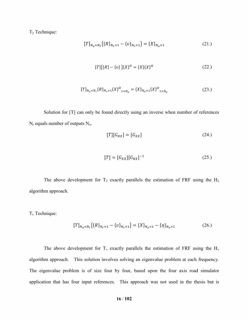
T2 Technique:
(21.)
(22.)
(23.)
Solution for [T] can only be found directly using an inverse when number of references
Nr equals number of outputs No.
(24.)
(25.)
The above development for T2 exactly parallels the estimation of FRF using the H2
algorithm approach.
Tv Technique:
(26.)
The above development for Tv exactly parallels the estimation of FRF using the Hv
algorithm approach. This solution involves solving an eigenvalue problem at each frequency.
The eigenvalue problem is of size four by four, based upon the four axis road simulator
application that has four input references. This approach was not used in the thesis but is

17 / 102
mentioned here for completeness. For more information, please see the MIMO FRF
development for the details of the eigenvalue solution approach[9] [8].
The T1 algorithm approach is the only approach used for the estimation of
transmissibility for this thesis. In general, for all three techniques, the four inputs (references)
used in the four axis road simulator must not be highly correlated. This means that the actual
measured motions at the four hydraulic actuators can be partially correlated but must not be
completely correlated at any frequency in the analysis band. It must be noted that this evaluation
must be made via the actual LVDT motions (references) measured at the four wheel pans for the
four axis road simulator application. In general, the excitation signals being sent to the input of
each hydraulic actuator will be completely uncorrelated random but, due to structural interaction
between the vehicle and the hydraulic actuators, the actual, measured input motions may be
partially correlated. This is not a problem as long as the interaction is not severe enough to cause
complete correlation at one or more frequencies. The use of singular value or eigenvalue
decomposition of the matrix, in the form of virtual references, is used during the
measurement process to be certain that this requirement is met.

18 / 102
Chapter 3. Vehicle Comparisons via Transmissibility Function
3.1 Test Setup
Figure 4: UC-SDRL Four Axis Road Simulator
Testing was performed in the UC-SDRL High Bay Laboratory on the UC-SDRL (MTS
320) Four Axis Road Simulator. The laboratory is equipped with a service lift for installation of
the vehicle on the four actuators (Model 248.03 Hydraulic Shakers). The service lift is mounted
on an isolation mass (25’x14’x9” Concrete Inertia Mass) fitted with embedded steel plates for
securing the actuators. The vehicle is secured to the actuator pans with heavy duty nylon straps.

19 / 102
The vehicle is typically instrumented with over 150 channels of acquisition which will be
detailed below in Section 0.
With the vehicle positioned on the lift, drive files are generated. ‘Drive files’ are
generated from supplied ‘Ride Files’ for the installed vehicle using an iterative process
performed by MATLAB® based SimTest ® software. Further discussion of this process can be
found in Section 3.2.The vendor supplied a myriad of ‘Ride Files’ for use in testing, including
‘Belgian Block’, ‘Cobble Stone’, ‘Gravel’, ‘Harshness’, ‘NVH 1’, ‘NVH 2’, and ‘NVH 3’. The
initial evaluation utilized these drive files until the correlation problem among the inputs
(references) was noted.
3.1.1 Vehicles Tested
Testing was performed for four distinct vehicles. The tests are referred to in the order
they were performed as Vehicle A, B, C, D, and E. Vehicle A was retested at a later date to
incorporate best practices and was then referred to as Vehicle D. Vehicle E is considered Best in
Class for this size vehicle based upon customer surveys, particularly with respect to NVH. Test
dates are tabulated in Table 1 below.
Table 1: Testing Dates
Test Dates Vehicle Type Notes
8/17/2006 Vehicle A Sedan
10/04/2006 - 10/12/2006 Vehicle B Coupe
10/26/2006 - 10/30/2006 Vehicle C Sedan
12/07/2006 - 1/11/2007 Vehicle D Sedan Repeat of Vehicle A
4/05/2007 - 4/11/2007 Vehicle E Sedan

20 / 102
3.1.2 Test Equipment
The intent of testing was to compare dissimilar vehicles. To accomplish this, it was
desirable to make similar measurements on each vehicle. This requires installing
instrumentation in analogous locations from one vehicle to the next (ex. Seat rail on each
vehicle, cross body beam on each vehicle, etc.). Due to variations in geometry this was, at times,
challenging. To aid in the organization of sensor locations and later comparisons a numbering
scheme was established that was continued for each subsequent vehicles (Table 2).
Table 2: Instrumentation Details
Figure 5: Input Numbering and Direction Definition
Numbering Scheme Installation Location Sensor Type Nominal Sensitivity Manufacturer Model
1-4 Integral to Hydraulic Shaker LVDT 3.34 V/in
10 Series Wheel Pans Uniaxial Accelerometer 1 V/G PCB UT333M07
20 Series Wheel Spindles Uniaxial Accelerometer 1 V/G PCB UT333M07
100/200 Series A-Pillar Triaxial Accelerometers 1 V/G PCB XT356B18
300/400 Series B-Pillar Triaxial Accelerometers 1 V/G PCB XT356B18
500 Series Bulkhead/Firewall Triaxial Accelerometers 1 V/G PCB XT356B18
600 Series Cross Body Beam Triaxial Accelerometers 1 V/G PCB XT356B18
700 Series Seat Rails Triaxial Accelerometers 1 V/G PCB XT356B18
800 Series Seated Dummies Microphones 20 mV/Pa Modal Shop 130A10/P10
900 Series Instrumentation Panel Triaxial Accelerometers 1 V/G PCB XT356B18
21 / 102
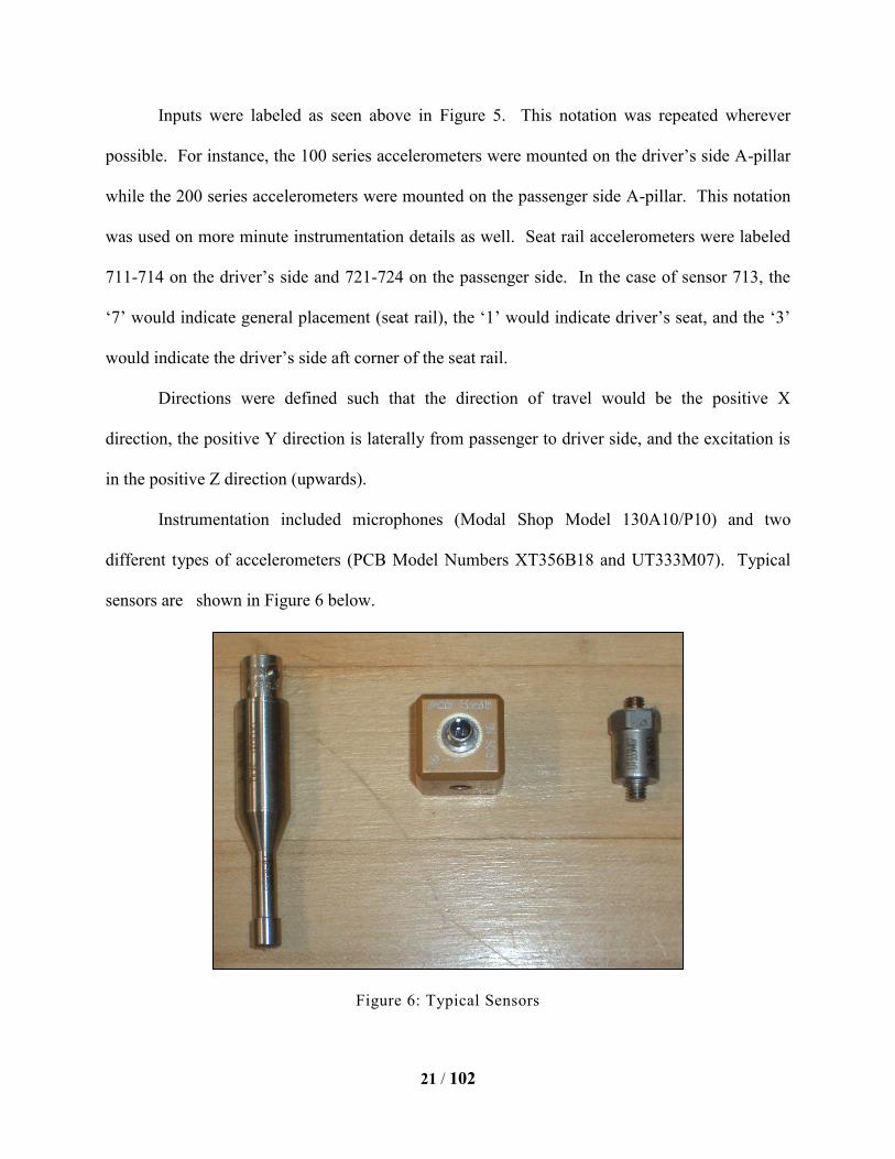
Inputs were labeled as seen above in Figure 5. This notation was repeated wherever
possible. For instance, the 100 series accelerometers were mounted on the driver’s side A-pillar
while the 200 series accelerometers were mounted on the passenger side A-pillar. This notation
was used on more minute instrumentation details as well. Seat rail accelerometers were labeled
711-714 on the driver’s side and 721-724 on the passenger side. In the case of sensor 713, the
‘7’ would indicate general placement (seat rail), the ‘1’ would indicate driver’s seat, and the ‘3’
would indicate the driver’s side aft corner of the seat rail.
Directions were defined such that the direction of travel would be the positive X
direction, the positive Y direction is laterally from passenger to driver side, and the excitation is
in the positive Z direction (upwards).
Instrumentation included microphones (Modal Shop Model 130A10/P10) and two
different types of accelerometers (PCB Model Numbers XT356B18 and UT333M07). Typical
sensors are shown in Figure 6 below.
Figure 6: Typical Sensors

22 / 102
Additional equipment is required for cable management, signal conditioning, and
acquisition. To aid in cable management numerous ‘break out’ (PCB) boxes are utilized at
various points around the vehicle. Signal conditioning is performed by PCB 441A101 power
supplies and data acquisition is performed by a VXI System (HP E8400 A with Agilent/VTI
Instruments 143x hardware). The acquisition mainframe with attached cabling for one of the test
configurations can be seen below in Figure 7. All computation of transmissibility and related
digital signal processing was accomplished with a custom MATLAB® script, included in
Appendix G that utilized the sensor calibration information in an associated Excel documentation
file. The Excel files for each of the Vehicles are included in Appendices A through E.
Figure 7 : Data Acquisition Mainframe

23 / 102
3.2 Discussion of Road Simulator Input Characteristics
Traditional use of four axis road simulators in automotive testing involves using
simulated road inputs for use in durability testing. These are generated by measuring response at
a number of locations on the vehicle as it travels over a given terrain. The measured responses
(referred to as the “ride files”) are then utilized in an iterative process, involving an inverse
calculation, to estimate a set of input files for all axes of the road simulator that will be used to
replicate the response as measured on the vehicle for the type of road input of interest (referred
to as the “drive file”). This numerical procedure estimates a drive file based upon the
characteristics and limitations of the specific road simulator being utilized. This numerical
procedure, however, does not constrain the resulting drive files (inputs to the individual
hydraulic actuators) to be uncorrelated and, experience with the UC-SDRL Four Axis Simulator
indicates that, these types of inputs are, at times, significantly correlated. This will be examined
further in Section 0.
While specific and measured vehicle responses, to a specific type of road surface, are
commonly used as the basis for determining the displacement inputs to each axis of the road
simulator when the system is used for durability or NVH studies, this will not be acceptable for
the MIMO transmissibility case. Instead, uncorrelated random inputs are used to drive each of
the four axes rather than using a drive file. Conventional drive file based data was taken for each
vehicle as a requirement from the research partner but, in the end, this data was of no use for the
transmissibility study. RMS levels of response at specified output response locations can be
used to achieve response levels similar to those found in the ride files, if necessary.

24 / 102
3.3 Test Execution
The test execution was controlled by using MTS FlexTest software which allowed for the
use of drive files and various general function generator type inputs (sine, random, etc.). The
research partner supplied a myriad of ride files for each vehicles (used to generate drive files) for
use in testing, including ‘Belgian Block’, ‘Cobble Stone’, ‘Gravel’, ‘Harshness’, ‘NVH 1’,
‘NVH 2’, and ‘NVH 3’. Drive files are generated from the ride files for each vehicle using a
commercial, MATLAB® based program called SimTest®. Additionally, for the transmissibility
study discussed in this thesis, each vehicle was tested with four random inputs generated by the
MTS FlexTest software at three different magnitudes of input (referred to as 50%, 75%, and
100%). In this situation, the MTS FlexTest software, together with the MTS four axis road
simulator hardware, was essentially a large, four axes, hydraulic shaker system with
independently controlled inputs for each of the four axes.
Vehicle D was subjected to additional random excitation testing to determine the effects
of various strapping conditions since data from the initial set of straps and data from the final set
of straps was available. Note that each vehicle was delivered for testing over a two to three week
time period and then returned to the research partner. Further testing of previous vehicles (B and
C) with the new retention straps was not possible.

25 / 102
3.4 Strapping Effects
The research partner supplying the various vehicles for test typically tests in an
unstrapped condition on shakers recessed into the floor in their facility. The UC-SDRL Four
Axis Road Simulator tests vehicles in an elevated configuration since the hydraulic actuators are
mounted on air suspension systems in the High Bay Laboratory. As such, strapping of the tire to
the wheel pan is required for safety of the operator and vehicle under test. The addition of
strapping will change the stiffness of the interaction of the wheel and the wheel pan. To assess
this effect, an analytical model of the Four Axis Road Simulator, with a representative lumped
mass vehicle model mounted on the Road Simulator, was developed. Note that this was
discussed with the research partner prior to any testing and, since relatively low frequency
comparisons were of greatest interest, was not deemed as a problem.
Figure 8: Comparison of Straps Old (Left) vs. New (Right)
However, during the course of testing, the original straps failed due to wear and required
replacement. Replacement straps were of a different type and tightening mechanism. See Figure
8 for comparison of new straps to old. This loading (stiffness constraint) was not likely
consistent with earlier testing. The model became useful in assessing this variation and defining
the frequency limits where the strapping stiffness had little effect.

26 / 102
3.5 Four Axis Road Simulator Analytical Model
A simplified analytical model of the UC-SDRL Four Axis Road Simulator, with a
lumped mass model of an automotive vehicle in position on the simulator, was developed in
MATLAB®. The model is a 20 degree of freedom, lumped mass model as shown in Figure 9.
The lumped mass parameters were chosen based upon the physical masses of the hydraulic
actuator components and the physical mass and lumped mass distribution of a representative
3000 pound automotive vehicle.
Lumped stiffness and damping parameters were chosen to give known modal
characteristics (frequencies and damping) of the various components. The first compression
mode of the shakers is at 75 Hz. This information combined with the mass of the shaker was
used to estimate the stiffness using the equation for undamped natural frequency.
(27.)
This was not an exacting process but an attempt was made to get reasonable agreement
between the model and measured transmissibilities in terms of magnitude and frequency
characteristics and trends. The script that is utilized for implementation of this model is included
in Appendix F.

27 / 102
Figure 9: Schematic of Vehicle Model
The various portions of the test setup are modeled as follows:
M1 = Mass of a shaker post
M2 = Un-sprung weight at each corner
M3 = Mass of front/rear vehicle
M4 = Mass of left/right vehicle
M0 = Various vehicle masses
Note that all similar masses were set equal for simplicity. There is no such requirement
in the model code found in Appendix F.

28 / 102
Model results will be presented in section 0 for various parts of the model including the
wheel spindle, driver’s side vehicle structure, and forward vehicle structure. In general,
transmissibility calculated from the FRFs of the model was compared to measured
transmissibility in order to evaluate general agreement. Then the strapping stiffness was varied
in the model to determine the affected frequency range. The conclusion was that the
transmissibility characteristics were relatively unchanged below 25 Hz and, therefore, the
transmissibility data with different strapping could be compared through 25 Hz. This also gave a
reasonable frequency limit that was used for all final comparisons when looking for positive and
negative trends between different vehicles.

29 / 102
3.5.1 Nominal Model Results
Figure 10: Driving Point Measurement Location
In the test configuration, an accelerometer was installed onto each wheel pan in order to
estimate driving point transmissibility measurements (see Figure 10). Figure 11 shows a
comparison of the driving point transmissibility measurement (right) to the driving point
transmissibility simulation from the nominal model condition (left).
Figure 11: Comparison of Model (left) to Driving Point Measurement (right)
0 5 10 15 20 25 3010
-4
10-2
100
102
Frequency (hz)
Magnitude (
g/in)
Driving Point Transmissibility
At The Wheel Pan
0 5 10 15 20 25 30
-180
-90
0
90
180
Frequency (hz)
Phase (
degre
es)
0 5 10 15 20 25 3010
-4
10-2
100
102
Magnitude (
g/in)
Frequency (Hz)
Transmissibility
O:R - 11:1
0 5 10 15 20 25 30-200
-100
0
100
200
Phase (
degre
es)
Frequency (Hz)
vehD75

30 / 102
Figure 12: Comparison of Model (left) to Wheel Spindle Measurement (right)
Figure 13: Comparison of Model (left) to Driver's Side Seat Rail Measurement (right)
Additional comparisons of the model transmissibilities to analogous test data can be seen
in Figure 12 and Figure 13 above. All magnitude units are g / inch and the trend characteristics
between model and test are in good agreement.
0 5 10 15 20 25 3010
-4
10-2
100
102
Frequency (hz)
Magnitude (
g/in)
Wheel/Wheelpan Transmissibility
0 5 10 15 20 25 30
-180
-90
0
90
180
Frequency (hz)
Phase (
degre
es)
0 5 10 15 20 25 3010
-4
10-2
100
102
Magnitude (
g/in)
Frequency (Hz)
Transmissibility
O:R - 21:1
0 5 10 15 20 25 30-200
-100
0
100
200
Phase (
degre
es)
Frequency (Hz)
vehD75
0 5 10 15 20 25 3010
-4
10-2
100
102
Frequency (hz)
Magnitude (
g/in)
Left Vehicle Structure/Wheelpan Transmissibility
0 5 10 15 20 25 30
-180
-90
0
90
180
Frequency (hz)
Phase (
degre
es)
0 5 10 15 20 25 3010
-4
10-2
100
102
Magnitude (
g/in)
Frequency (Hz)
Transmissibility
O:R - 711:1
0 5 10 15 20 25 30-200
-100
0
100
200
Phase (
degre
es)
Frequency (Hz)
vehD75

31 / 102
3.5.2 Modeling Variable Strap Stiffness
As mentioned previously, in the course of testing, the vehicle retention straps broke.
Exact duplicates could not be sourced, so another type of strap was substituted. The replacement
straps had a different tightening mechanism and did not likely produce tightness consistent with
the original straps. To assess the difference in strap tightness, the stiffness of the post-tire
contact (K2) was varied.
Figure 14: Effect of Strap Stiffness
From Figure 14, several conclusions were drawn. First, there is almost no effect of the
strapping stiffness below 15 Hz, in either magnitude or phase. Second, when comparing
transmissibilities, magnitude effects are of primary interest. Significantly different
transmissibility magnitudes mean that the structures being compared will be much stiffer (with
0 10 20 30 40 50 60 70 80 90 10010
-2
100
102
Frequency (hz)
Magnitude (
g/in)
Wheel/Wheelpan Transmissibility
0 10 20 30 40 50 60 70 80 90 100
-180
-90
0
90
180
Frequency (hz)
Phase (
degre
es)

32 / 102
less transmissibility) or less stiff (with greater transmissibility). Since measured
transmissibilities exist for Vehicle D with both the original retention straps and the new retention
straps, the retention strap tension was adjusted to get the best match possible for further testing.
If only magnitudes are of interest, then the usable frequency range can be extended to 20 or even
25 Hz.
3.6 Transmissibility Results
Transmissibility data was compared from 0-30 Hz across all vehicles. Several samples of
transmissibility data are provided below in Section 4.4.2. For a more comprehesive comparison
of transmissability for various vehicles, input levels and grouping, etc, please see the companion
thesis [1].

33 / 102
3.6.1 Drive File Excitation
As discussed above, transmissibility calculations have a requirement that the inputs be
uncorrelated. Upon examination of the virtual references for the various drive file cases, there
were numerous examples where the four inputs were significantly correlated. The example in
Figure 15 (left) shows a Belgian block drive file case where all four shakers are active, but there
are only three independent excitations within the four excitation drive signals. This is compared
to a random excitation case (right) in which all four inputs are uncorrelated.
Figure 15: Comparison of Correlated (Left) and Uncorrelated (Right) Inputs
While some drive cases yielded acceptable inputs over the frequency range of interest,
several drive files yielded only two or three (as in the above example) independent inputs instead
of the required four. For this reason, while input-output data was taken for each vehicle for all
drive file cases, transmissibilities were not estimated from this data and this data was not used
for further analysis.
0 10 20 30 40 50 60 70 80 90 10010
-12
10-10
10-8
10-6
10-4
10-2
100
Principal References
Veh_A_2500_BB_Dx2006_0817_1623.sdf
Frequency (hz)
Magnitude (
g/in)2
0 10 20 30 40 50 60 70 80 90 10010
-12
10-10
10-8
10-6
10-4
10-2
100
Principal References
Veh_D_2500_Rand_Dx2007_0104_1554b(100%).sdf
Frequency (hz)
Magnitude (
g/in)2
34 / 102
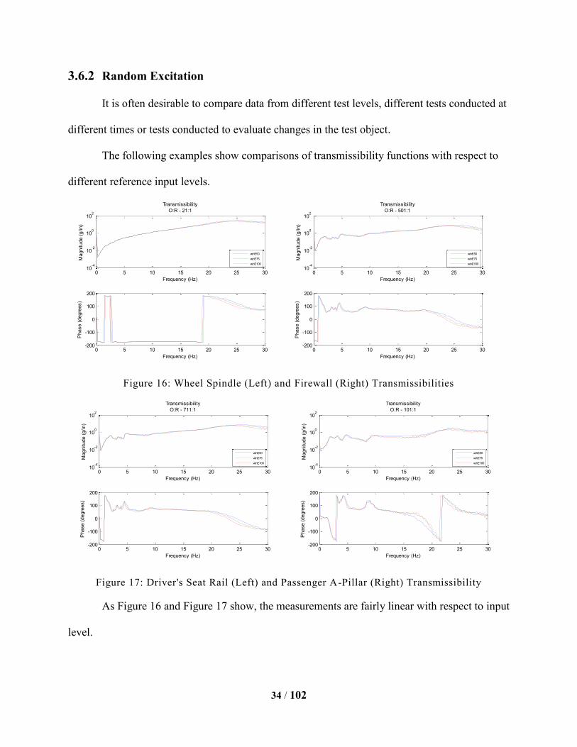
3.6.2 Random Excitation
It is often desirable to compare data from different test levels, different tests conducted at
different times or tests conducted to evaluate changes in the test object.
The following examples show comparisons of transmissibility functions with respect to
different reference input levels.
Figure 16: Wheel Spindle (Left) and Firewall (Right) Transmissibilities
Figure 17: Driver's Seat Rail (Left) and Passenger A-Pillar (Right) Transmissibility
As Figure 16 and Figure 17 show, the measurements are fairly linear with respect to input
level.
0 5 10 15 20 25 3010
-4
10-2
100
102
Magnitude (
g/in)
Frequency (Hz)
Transmissibility
O:R - 21:1
0 5 10 15 20 25 30-200
-100
0
100
200
Phase (
degre
es)
Frequency (Hz)
vehE50
vehE75
vehE100
0 5 10 15 20 25 3010
-4
10-2
100
102
Magnitude (
g/in)
Frequency (Hz)
Transmissibility
O:R - 501:1
0 5 10 15 20 25 30-200
-100
0
100
200P
hase (
degre
es)
Frequency (Hz)
vehE50
vehE75
vehE100
0 5 10 15 20 25 3010
-4
10-2
100
102
Magnitude (
g/in)
Frequency (Hz)
Transmissibility
O:R - 711:1
0 5 10 15 20 25 30-200
-100
0
100
200
Phase (
degre
es)
Frequency (Hz)
vehE50
vehE75
vehE100
0 5 10 15 20 25 3010
-4
10-2
100
102
Magnitude (
g/in)
Frequency (Hz)
Transmissibility
O:R - 101:1
0 5 10 15 20 25 30-200
-100
0
100
200
Phase (
degre
es)
Frequency (Hz)
vehE50
vehE75
vehE100

35 / 102
Another potential use for transmissibilities is comparisons of similar structures. Figure
18 and Figure 19 below show a comparison of transmissibilities among the various vehicles
tested.
Figure 18:Wheel Spindle (Left) and Firewall (Right) Transmissibilities
Figure 19: Driver's Seat Rail (Left) and Passenger A-Pillar (Right) Transmissibility
Figure 20 and Figure 21 below show a comparison of transmissibilities for various
strapping conditions on Vehicle D.
0 5 10 15 20 25 3010
-4
10-2
100
102
Magnitude (
g/in)
Frequency (Hz)
Transmissibility
O:R - 21:1
0 5 10 15 20 25 30-200
-100
0
100
200
Phase (
degre
es)
Frequency (Hz)
vehB75
vehC75
vehD75
vehE75
0 5 10 15 20 25 3010
-4
10-2
100
102
Magnitude (
g/in)
Frequency (Hz)
Transmissibility
O:R - 501:1
0 5 10 15 20 25 30-200
-100
0
100
200
Phase (
degre
es)
Frequency (Hz)
vehB75
vehC75
vehD75
vehE75
0 5 10 15 20 25 3010
-5
100
105
Magnitude (
g/in)
Frequency (Hz)
Transmissibility
O:R - 711:4
0 5 10 15 20 25 30-200
-100
0
100
200
Phase (
degre
es)
Frequency (Hz)
vehB75
vehC75
vehD75
vehE75
0 5 10 15 20 25 3010
-4
10-2
100
102
Magnitude (
g/in)
Frequency (Hz)
Transmissibility
O:R - 101:1
0 5 10 15 20 25 30-200
-100
0
100
200
Phase (
degre
es)
Frequency (Hz)
vehB75
vehC75
vehD75
vehE75

36 / 102
Figure 20: Spindle (Left) and Firewall (Right) Transmissibilities for Various Strap Conditions
Figure 21: Seat Rail (Left) and A-Pillar (Right) Transmissibilities for Various Strap Conditions
The above plots confirm the strapping stiffness has little to no effect on transmissibility
magnitude below 15 Hz and very little effect on phase. Note that this is consistent with the
model results in Section 3.5.2.
0 5 10 15 20 25 3010
-4
10-2
100
102
Magnitude (
g/in)
Frequency (Hz)
Transmissibility
O:R - 21:1
0 5 10 15 20 25 30-200
-100
0
100
200
Phase (
degre
es)
Frequency (Hz)
vehD75
vehD_FLRR_on_75
vehD_FRRL_on_75
vehD_leftside_on_75
vehD_rightside_on_75
0 5 10 15 20 25 3010
-4
10-2
100
102
Magnitude (
g/in)
Frequency (Hz)
Transmissibility
O:R - 501:1
0 5 10 15 20 25 30-200
-100
0
100
200
Phase (
degre
es)
Frequency (Hz)
vehD75
vehD_FLRR_on_75
vehD_FRRL_on_75
vehD_leftside_on_75
vehD_rightside_on_75
0 5 10 15 20 25 3010
-4
10-2
100
102
Magnitude (
g/in)
Frequency (Hz)
Transmissibility
O:R - 711:1
0 5 10 15 20 25 30-200
-100
0
100
200
Phase (
degre
es)
Frequency (Hz)
vehD75
vehD_FLRR_on_75
vehD_FRRL_on_75
vehD_leftside_on_75
vehD_rightside_on_75
0 5 10 15 20 25 3010
-4
10-2
100
102
Magnitude (
g/in)
Frequency (Hz)
Transmissibility
O:R - 101:1
0 5 10 15 20 25 30-200
-100
0
100
200
Phase (
degre
es)
Frequency (Hz)
vehD75
vehD_FLRR_on_75
vehD_FRRL_on_75
vehD_leftside_on_75
vehD_rightside_on_75

37 / 102
Chapter 4. Principal Component Analysis in Structural Dynamics
Much of the material of this chapter was originally published as a paper for the
International Modal Analysis Conference [7]. The version originally published inadvertently
included some acoustic measurements in the principal component analysis (PCA) calculations,
which skewed the results. The data shown below has had the acoustic data removed. Some of
the other PCA examples from this paper were reprocessed in the following sections of the thesis
using transmissibility data from the testing of Vehicles B, C, D and E to be more relevant to the
automotive testing situation.
4.1 Introduction
The concept of identifying the various underlying linear contributors in a set of data is
needed in many fields of science and engineering. The techniques have been independently
developed and/or discovered by many authors in many completely different application areas.
Many times the procedure has acquired a different name depending upon the individual or
specific application focus. This has resulted in a confusing set of designations for fundamentally
similar techniques: Principal Component Analysis (PCA), Independent Component Analysis
(ICA), Complex Mode Indicator Function (CMIF), Principal Response Functions, Principal
Gains, and others. Without detracting from the insight and ingenuity of each of the original
developers, each of these techniques relies upon the property of the singular value decomposition
(SVD) to represent a set of functions as a product of weighting factors and independent linear
contributions. Today, this is known more widely as the SVD approach to principal component
analysis (PCA).

38 / 102
4.2 Nomenclature
Nr = Number of inputs (references)
No = Number of outputs.
Nf = Number of frequencies.
NS = Short matrix dimension.
NL = Long matrix dimension.
= Frequency (rad/sec).
r = Complex modal frequency
[B] = Generic data matrix.
[H()] = Frequency response function matrix (No x Ni).
[T()] = Transmissibility function matrix (No x Nr)).
[GRR()] = Force cross power spectra matrix (Nr x Nr).
[U] = Left singular vector matrix.
[S] = Principal value matrix (diagonal).
[] = Singular value matrix (diagonal).
[] = Eigenvalue matrix (diagonal).
[V] = Right singular vector, or eigenvector, matrix.

39 / 102
4.3 Background
Principal component analysis (PCA) is the general description for a number of
multivariate data analysis methods that typically provide a linear transformation from a set of
physical variables to a new set of virtual variables. The linear transformation is in the form of a
set of orthonormal vectors (principal vectors) and associated scaling for the orthonormal vectors
(principal values). These scaling terms are often thought of as the weight or importance of the
associated orthonormal vectors since the orthonormal vectors have no overall scaling (unity
length) but are orthogonal to one another (have no projection or relationship to one another).
While there are many approaches to computing the principal components, most modern
implementations utilize eigenvalue decomposition (ED) methods for the square matrix case and
singular value decomposition (SVD) for the rectangular matrix case.
Historically, the primary governing equation for the decomposition is as follows:
(28.)
In this relationship, the common form starts with a data matrix ([B]) that is frequently real-
valued and square which is transformed by the orthonormal vectors ([U]) and the diagonal
principal value matrix. The form of the SVD equation given in Equation (28) is referred to as
the economical form of the SVD. Since the orthonormal vectors have no scaling (unity length),
the principal values contain the physical scaling of the original data matrix ([B]). The scaling
nature of the principal or singular values gives rise to the term principal gain that is occasionally
found in structural dynamics.
With respect to structural dynamics, the PCA is frequently performed time by time, or
frequency by frequency, across a data matrix that is square or rectangular at each time or

40 / 102
frequency. The common form of the PCA concept when developed via the singular value
decomposition of a complex-valued data matrix becomes:
(29.)
In this version of the relationship, still the economical from of the SVD, the common form starts
with a data matrix ([B]) that is frequently complex-valued and rectangular which is transformed
by the orthonormal vectors ([U]) and [V]) and the diagonal principal value matrix ([S]). If the
data matrix ([B]) is complex valued, it is important to note that the phasing between the left
principal vector ([U]) and the associated right principal vector ([V]) is generally not unique. If
the principal vectors are used independently (left or right singular vectors) this arbitrary phase
issue must be accounted for.
Plotting the principal values, largest to smallest across the time or frequency range,
results in a 2-D scaling function that is often used to determine specific time dependent or
frequency dependent features in the data without the need to look at individual measurements.
This can be tremendously helpful when the number of terms in the data matrix (rows and
columns) is large.
The PCA techniques were first developed in the early 1900s but did not come into
common use in structural dynamics until the 1970s and 1980s with the advent of math packages
like EISPACK® and LINPACK® and subsequent development of user friendly software like
Mathmatica® and MATLAB®. A number of textbooks are now available that discuss these
methods but many of the available texts do not include complex valued, spectral analysis that is
common to structural dynamics data [5][6] [10][11][12][13][14][15].
PCA methods have found common usage in many science and engineering areas. The
most common applications involve multidimensional scaling, linear modeling, data quality

41 / 102
analysis and analysis of variance. These are the same applications that make the general PCA
methods so attractive to structural dynamics. Since much of structural analysis is built upon
linearity, super-position and linear expansion, the PCA methods have found wide and increasing
use, particularly in the experimental data analysis areas of structural dynamics. Common uses
are the evaluation of force independence in the multiple input, multiple output (MIMO)
estimation of frequency response functions (FRFs), the evaluation of close and repeated modal
frequencies in the MIMO FRF matrix using a method that is known as the complex mode
indicator function (CMIF) and the development of virtual FRF functions known as principal
response functions.
4.4 Common Applications
With respect to structural dynamics, at least three PCA based methods are relatively well
known and frequently utilized. The principal force analysis associated with MIMO FRF
estimation, the close or repeated mode analysis of the complex mode indicator function (CMIF)
and the virtual FRF estimation related to principal response functions have all been used for ten
or more years and are summarized in the following sections.

42 / 102
4.4.1 Principal (Virtual) References
The current approach used to evaluate correlated inputs for the MIMO transmissibility or
FRF estimation problem involves utilizing principal component analysis to determine the
number of contributing references (principal or virtual references) to the [GRR] matrix
[16][17][18]. The [GRR] matrix is the cross power spectra matrix involving all the multiple,
simultaneous reference inputs applied to the structure during the MIMO transmissibility or FRF
estimation. In this approach, the matrix that must be evaluated is:
(30.)
This application of PCA involves an eigenvalue decomposition of the [GRR] matrix at each
frequency of the measured power spectra of the inputs (references). Since the eigenvectors of
such a decomposition are unitary, the eigenvalues should all be of approximately the same size if
each of the inputs is contributing to the excitation of the structure equally. If one of the
eigenvalues is much smaller at a particular frequency, one of the inputs is not present or one of
the inputs is correlated with the other input(s) at that frequency.
(31.)
[] in the above equation represents the eigenvalues of the [GRR] matrix. If any of the
eigenvalues of the [GRR] matrix are zero or insignificant, then the [GRR] matrix is singular.
Therefore, for a four input test, the [GRR] matrix is 4x4 at each frequency and should have four
eigenvalues at each frequency. (The number of significant eigenvalues is the number of
uncorrelated inputs).

43 / 102
Figure 22: Principal (Virtual) Reference Spectrum – Random Excitation
Figure 22 shows the principal reference plots for a four input random excitation case.
These principal reference curves are no longer linked to a specific physical exciter location due
to the linear transformation involved. These curves are sometimes referred to as virtual inputs.
Note that the overall difference in the four curves is typically one or two orders of magnitudes
and there will be some fluctuation in the curves in the frequency region where there are lightly
damped modes due to the exciter-structure interaction.
0 10 20 30 40 50 60 70 80 90 10010
-12
10-10
10-8
10-6
10-4
10-2
100
Principal References
Veh_D_2500_Rand_Dx2007_0104_1554b(100%).sdf
Frequency (hz)
Magnitude (
g/in)2
44 / 102
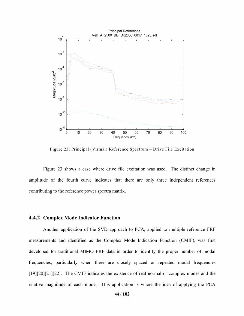
Figure 23: Principal (Virtual) Reference Spectrum – Drive File Excitation
Figure 23 shows a case where drive file excitation was used. The distinct change in
amplitude of the fourth curve indicates that there are only three independent references
contributing to the reference power spectra matrix.
4.4.2 Complex Mode Indicator Function
Another application of the SVD approach to PCA, applied to multiple reference FRF
measurements and identified as the Complex Mode Indication Function (CMIF), was first
developed for traditional MIMO FRF data in order to identify the proper number of modal
frequencies, particularly when there are closely spaced or repeated modal frequencies
[19][20][21][22]. The CMIF indicates the existence of real normal or complex modes and the
relative magnitude of each mode. This application is where the idea of applying the PCA
0 10 20 30 40 50 60 70 80 90 10010
-12
10-10
10-8
10-6
10-4
10-2
100
Principal References
Veh_A_2500_BB_Dx2006_0817_1623.sdf
Frequency (hz)
Magnitude (
g/in)2

45 / 102
technique to transmissibility measurements from the four axis road simulator originates. Since
each transmissibility matrix will always contain four references, and the economical SVD will
generate four curves, comparison between and among vehicles or test conditions can be easily
made, although no direct relationship to modal contribution is expected.
The CMIF is defined as the economical (function of the short dimension) singular values,
computed from the MIMO FRF matrix at each spectral line. The CMIF is the plot of these
singular values, typically on a log magnitude scale, as a function of frequency. The peaks
detected in the CMIF plot indicate a normalized response dominated by one or more significant
contributions; therefore, the existence of modes, and the corresponding frequencies of these
peaks give the damped natural frequencies for each mode. In this way, the CMIF is using the
PCA approach to take advantage of the superposition principle commonly known as the
expansion theorem. In the application of the CMIF to traditional modal parameter estimation
algorithms, the number of modes detected in the CMIF determines the minimum number of
degrees-of-freedom of the system equation for the algorithm. A number of additional degrees-of-
freedom may be needed to take care of residual effects and noise contamination.
(32.)
Most often, the number of input points (reference points), Nr, is less than the number of
response points, No. In the above equation, if the number of effective modes at a given frequency
is less than or equal to the smaller dimension of the FRF matrix, , the singular value
decomposition leads to approximate mode shapes (left singular vectors) and approximate modal
participation factors (right singular vectors). The singular value is then equivalent to the scaling
factor Qr divided by the difference between the discrete frequency and the modal frequency j-
r. For a given mode, since the scaling factor is a constant, the closer the modal frequency is to

46 / 102
the discrete frequency, the larger the singular value will be. Therefore, the damped natural
frequency is the frequency at which the maximum magnitude of the singular value occurs. If
different modes are compared, the stronger the modal contribution (larger residue value), the
larger the singular value will be. The peak in the CMIF indicates the location on the frequency
axis that is nearest to the pole. The frequency is the estimated damped natural frequency, to
within the accuracy of the frequency resolution.
Figure 24:Complex Mode Indicator Function (CMIF)
Since the mode shapes that contribute to each peak do not change much around each
peak, several adjacent spectral lines from the FRF matrix can be used simultaneously for a better
estimation of mode shapes. By including several spectral lines of data in the singular value
decomposition calculation, the effect of the leakage error can be minimized. If only the
quadrature (imaginary) part of the FRF matrix is used in CMIF, the singular values will be much
more distinct.

47 / 102
4.4.3 Principal Response Functions
Similar in concept to the CMIF is the development of the Principal Response Functions
(PRF) [23][24][25]. In this case, however, instead of performing the decomposition of the FRF
data matrix frequency by frequency, the entire data matrix is arranged in two dimensions such
that each column contains a single FRF and the singular value decomposition is then performed
on this new data matrix.
(33.)
It was then recognized that the left singular vectors [U] are a function of frequency and
contain the primary spectral characteristics and the singular values [] the relative contribution
of those vectors to the global data matrix. By selecting only the 'r' most significant singular
values and associated left singular vectors, the principal response functions are then defined as:
(34.)
The principal response functions reveal the nature of the noise and noise floor contained
in the data and, contrary to normal intuition, demonstrates that more data is not always better.
Once the real information in the data matrix is identified, the addition of more measurements can
only contribute to the noise and hence effectively raises the noise floor and makes parameter
identification more difficult.
In the following example, the transmissibility matrix [T] is used in place of the FRF
matrix [H]. The following two plots in Figure 25 reveal for vehicle B that, although there are
624 individual transmissibility measurements (154x4), only about 25 PRFs are necessary to
explain the spectral information for the top four orders of magnitude of transmissibility. The left
figure is the plot of the top 25 PRFs; the right figure is the top 300 PRFs. It becomes clear by
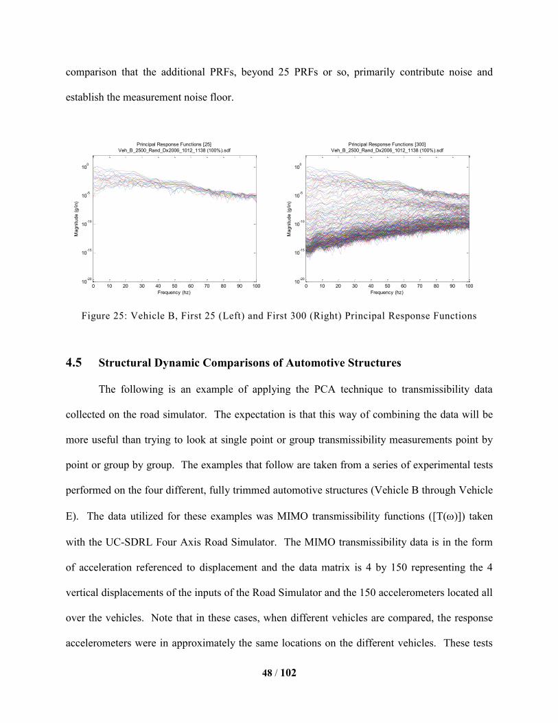
48 / 102
comparison that the additional PRFs, beyond 25 PRFs or so, primarily contribute noise and
establish the measurement noise floor.
Figure 25: Vehicle B, First 25 (Left) and First 300 (Right) Principal Response Functions
4.5 Structural Dynamic Comparisons of Automotive Structures
The following is an example of applying the PCA technique to transmissibility data
collected on the road simulator. The expectation is that this way of combining the data will be
more useful than trying to look at single point or group transmissibility measurements point by
point or group by group. The examples that follow are taken from a series of experimental tests
performed on the four different, fully trimmed automotive structures (Vehicle B through Vehicle
E). The data utilized for these examples was MIMO transmissibility functions ([T()]) taken
with the UC-SDRL Four Axis Road Simulator. The MIMO transmissibility data is in the form
of acceleration referenced to displacement and the data matrix is 4 by 150 representing the 4
vertical displacements of the inputs of the Road Simulator and the 150 accelerometers located all
over the vehicles. Note that in these cases, when different vehicles are compared, the response
accelerometers were in approximately the same locations on the different vehicles. These tests
0 10 20 30 40 50 60 70 80 90 10010
-20
10-15
10-10
10-5
100
Principal Response Functions [25]
Veh_B_2500_Rand_Dx2006_1012_1138 (100%).sdf
Frequency (hz)
Magnitude (
g/in)
0 10 20 30 40 50 60 70 80 90 10010
-20
10-15
10-10
10-5
100
Principal Response Functions [300]
Veh_B_2500_Rand_Dx2006_1012_1138 (100%).sdf
Frequency (hz)M
agnitude (
g/in)

49 / 102
were conducted to compare and contrast vehicles that were in the same general class (in terms of
size) but with clearly different characteristics, identified based upon owner feedback [1] [26].
4.5.1 Evaluation of Linearity/Time Variance/Repeatability
Comparing the principal components of a set of MIMO transmissibility data from
different test levels, different tests conducted at different times or tests conducted to evaluate
changes in the test object are good examples of the application of principal component analysis
methods. The following examples use the SVD approach to PCA to evaluate changes in the
transmissibility data matrix to different reference input levels. It is much easier to compare the
principal values as a function of frequency for the entire data set rather than to compare specific
measurement DOFs. In all of the following examples, all principal value curves are first
compared, followed by a comparison of only the primary principal value curves and then only
the secondary principal value curves.
In the following example, it is relatively easy to see that the response of Vehicle B, as
measured by all of the transmissibilities for three different excitation levels is relatively
independent of excitation level.

50 / 102
Figure 26: Vehicle B, Three input levels, All Data, All Principal Components
Figure 27: Vehicle B, Three input levels, All Data, Primary and Secondary Principal
Components
The next figures show the same information for Vehicle E for the same excitation
evaluation.
0 5 10 15 20 25 3010
-5
10-4
10-3
10-2
10-1
Principal Component Analysis
Frequency [Hz]
Magnitude (
g/in)
0 5 10 15 20 25 3010
-5
10-4
10-3
10-2
10-1
Frequency [Hz]
Magnitude (
g/in)
Principal Component #1
1.000 0.996 0.993
0.996 1.000 0.999
0.993 0.999 1.000
Veh B - 50%
Veh B - 75%
Veh B - 100%
0 5 10 15 20 25 3010
-5
10-4
10-3
10-2
10-1
Frequency [Hz]
Magnitude (
g/in)
Principal Component #2
1.000 0.999 0.997
0.999 1.000 1.000
0.997 1.000 1.000
Veh B - 50%
Veh B - 75%
Veh B - 100%

51 / 102
Figure 28: Vehicle E, Three input levels, All Data, All Principal Components
Figure 29: Vehicle E, Three input levels, All Data, Primary and Secondary Principal
Components
Figure 26 through Figure 29 show random excitation at three different magnitudes. The
similarity of the three curves demonstrates that the system (test apparatus with installed vehicle)
is linear with regard to input magnitude. Although it appears both vehicles are fairly linear, it
0 5 10 15 20 25 3010
-5
10-4
10-3
10-2
10-1
Principal Component Analysis
Frequency [Hz]
Magnitude (
g/in)
0 5 10 15 20 25 3010
-5
10-4
10-3
10-2
10-1
Frequency [Hz]
Magnitude (
g/in)
Principal Component #1
1.000 1.000 1.000
1.000 1.000 1.000
1.000 1.000 1.000
Veh E - 50%
Veh E - 75%
Veh E - 100%
0 5 10 15 20 25 3010
-5
10-4
10-3
10-2
10-1
Frequency [Hz]
Magnitude (
g/in)
Principal Component #2
1.000 0.973 0.984
0.973 1.000 0.998
0.984 0.998 1.000
Veh E - 50%
Veh E - 75%
Veh E - 100%

52 / 102
appears Vehicle E has a stronger linear relationship (since the principal value curves more
closely match). Although this comparison has a limited sample size, it also suggests that the
testing has good repeatability.
Note that this method allows the analyst to get a measure of system linearity without
examining each of the 624 individual transmissibility measurements (154 x 4).
4.5.2 Evaluation of Test Parameters
During testing of a series of vehicles, the straps used to restrain the vehicle with respect
to the four actuators of the UC-SDRL Four Axis Road Simulator were damaged and could not be
used in further testing. The straps were replaced but the new straps were in a different
configuration as well as being of different sizes. The SVD approach to PCA was utilized to
evaluate both the before and after variation of the MIMO transmissibility data as well as to take a
further look at the effects of using one or more straps to restrain the vehicle.

53 / 102
Figure 30: Vehicle D, Various Strap Conditions, All Data, All Principal Components
Figure 31: Vehicle D, Various Strap Conditions, All Data, Primary and Secondary Principal
Components
From Figure 30 and Figure 31, several conclusions were drawn. First, these plots
confirm the model predictions that there is very little effect of the strapping stiffness below 15
0 5 10 15 20 25 3010
-5
10-4
10-3
10-2
10-1
Principal Component Analysis
Frequency [Hz]
Magnitude (
g/in)
0 5 10 15 20 25 3010
-5
10-4
10-3
10-2
10-1
Frequency [Hz]
Magnitude (
g/in)
Principal Component #1
1.000 0.993 0.982 0.945
0.993 1.000 0.989 0.946
0.982 0.989 1.000 0.976
0.945 0.946 0.976 1.000
Veh D - 3 Straps
Veh D - 2 Straps
Veh D - 1 Straps
Veh D - 0 Straps
0 5 10 15 20 25 3010
-5
10-4
10-3
10-2
10-1
Frequency [Hz]
Magnitude (
g/in)
Principal Component #2
1.000 0.995 0.966 0.954
0.995 1.000 0.975 0.957
0.966 0.975 1.000 0.980
0.954 0.957 0.980 1.000
Veh D - 3 Straps
Veh D - 2 Straps
Veh D - 1 Straps
Veh D - 0 Straps

54 / 102
Hz. Additionally, above 15 Hz, the primary principal value curves are not affected unless no
straps or only one strap is installed. This was not anticipated.
4.5.3 Directional Scaling
Frequently, the dominant direction of response is not clear when working with fully
trimmed vehicles and particularly vehicle subcomponents. The SVD approach to PCA can be
used to compare the overall scaling of the response from X to Y to Z direction in the data. In the
following examples (Figure 32 and Figure 33), the scaling of the Z direction can be seen to be at
a higher level that the X and Y directions. The original paper[7] (on which this section is based)
noted that the Z direction was much lower than the X and Y directions. This was due to the
erroneous inclusion of high magnitude microphone data which was coded in the X and Y
directions.
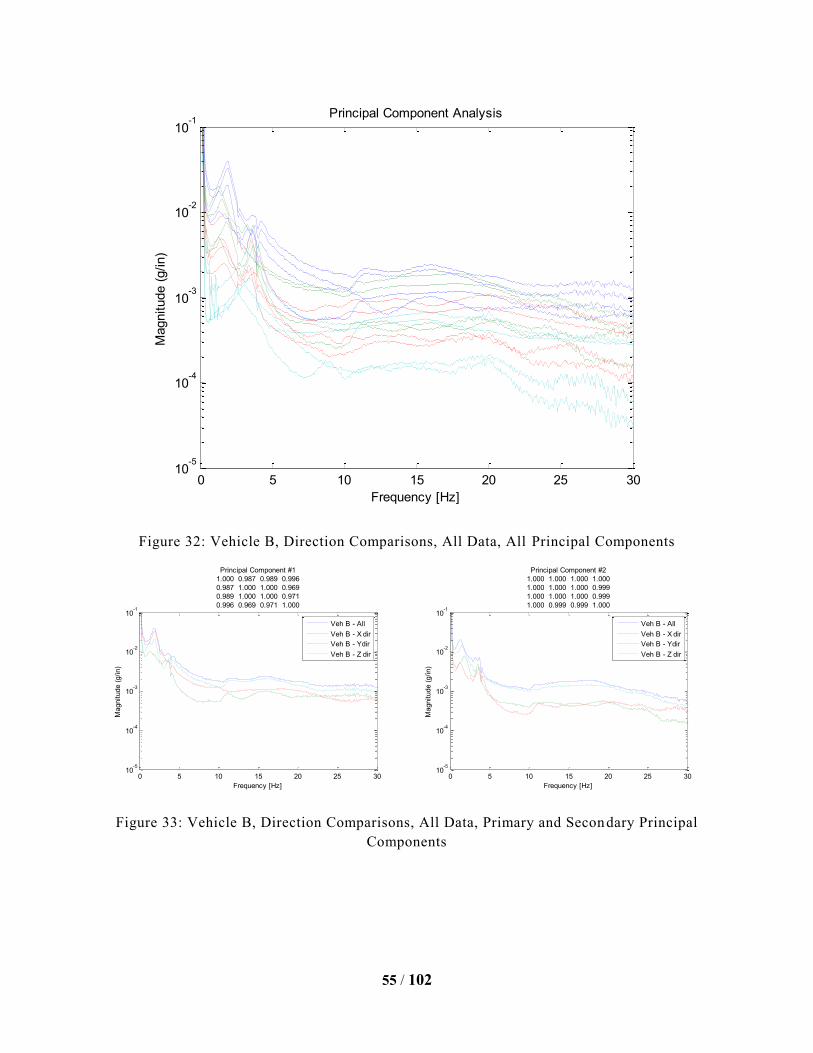
55 / 102
Figure 32: Vehicle B, Direction Comparisons, All Data, All Principal Components
Figure 33: Vehicle B, Direction Comparisons, All Data, Primary and Secondary Principal
Components
0 5 10 15 20 25 3010
-5
10-4
10-3
10-2
10-1
Principal Component Analysis
Frequency [Hz]
Magnitude (
g/in)
0 5 10 15 20 25 3010
-5
10-4
10-3
10-2
10-1
Frequency [Hz]
Magnitude (
g/in)
Principal Component #1
1.000 0.987 0.989 0.996
0.987 1.000 1.000 0.969
0.989 1.000 1.000 0.971
0.996 0.969 0.971 1.000
Veh B - All
Veh B - X dir
Veh B - Ydir
Veh B - Z dir
0 5 10 15 20 25 3010
-5
10-4
10-3
10-2
10-1
Frequency [Hz]
Magnitude (
g/in)
Principal Component #2
1.000 1.000 1.000 1.000
1.000 1.000 1.000 0.999
1.000 1.000 1.000 0.999
1.000 0.999 0.999 1.000
Veh B - All
Veh B - X dir
Veh B - Ydir
Veh B - Z dir
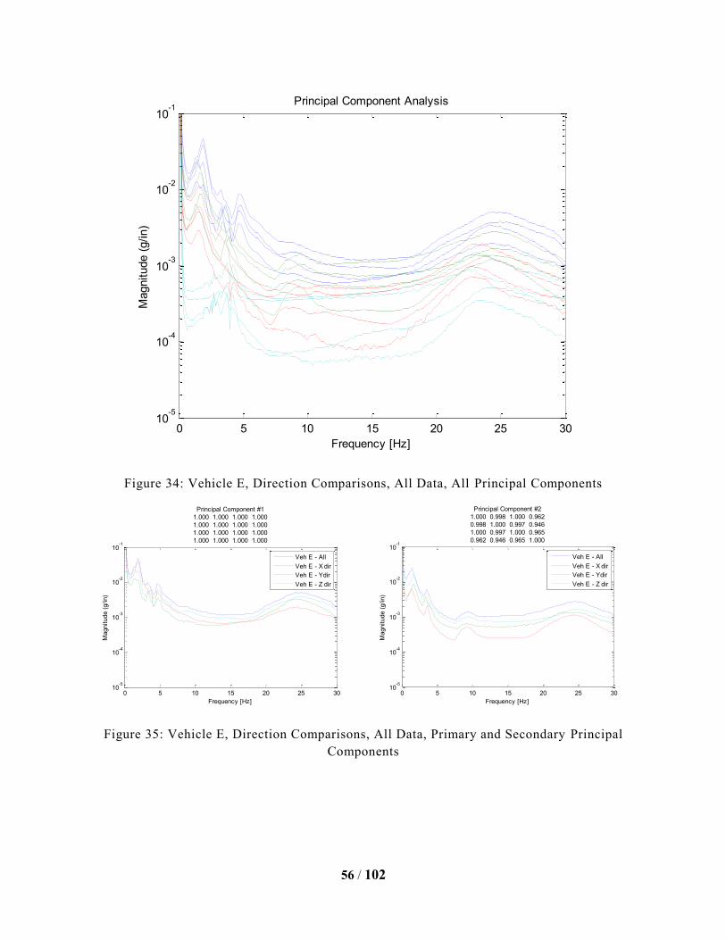
56 / 102
Figure 34: Vehicle E, Direction Comparisons, All Data, All Principal Components
Figure 35: Vehicle E, Direction Comparisons, All Data, Primary and Secondary Principal
Components
0 5 10 15 20 25 3010
-5
10-4
10-3
10-2
10-1
Principal Component Analysis
Frequency [Hz]
Magnitude (
g/in)
0 5 10 15 20 25 3010
-5
10-4
10-3
10-2
10-1
Frequency [Hz]
Magnitude (
g/in)
Principal Component #1
1.000 1.000 1.000 1.000
1.000 1.000 1.000 1.000
1.000 1.000 1.000 1.000
1.000 1.000 1.000 1.000
Veh E - All
Veh E - X dir
Veh E - Ydir
Veh E - Z dir
0 5 10 15 20 25 3010
-5
10-4
10-3
10-2
10-1
Frequency [Hz]
Magnitude (
g/in)
Principal Component #2
1.000 0.998 1.000 0.962
0.998 1.000 0.997 0.946
1.000 0.997 1.000 0.965
0.962 0.946 0.965 1.000
Veh E - All
Veh E - X dir
Veh E - Ydir
Veh E - Z dir

57 / 102
Figure 36: All Vehicles, X Direction Data, All Principal Components
Figure 37: All Vehicles, X Direction Data, Primary and Secondary Principal Components
0 5 10 15 20 25 3010
-5
10-4
10-3
10-2
10-1
Principal Component Analysis
Frequency [Hz]
Magnitude (
g/in)
0 5 10 15 20 25 3010
-5
10-4
10-3
10-2
10-1
Frequency [Hz]
Magnitude (
g/in)
Principal Component #1
1.000 1.000 1.000 1.000
1.000 1.000 1.000 1.000
1.000 1.000 1.000 1.000
1.000 1.000 1.000 1.000
Veh B - X Dir
Veh C - X Dir
Veh D - X Dir
Veh E - X Dir
0 5 10 15 20 25 3010
-5
10-4
10-3
10-2
10-1
Frequency [Hz]
Magnitude (
g/in)
Principal Component #2
1.000 0.988 0.991 0.999
0.988 1.000 0.999 0.990
0.991 0.999 1.000 0.992
0.999 0.990 0.992 1.000
Veh B - X Dir
Veh C - X Dir
Veh D - X Dir
Veh E - X Dir

58 / 102
Figure 38: All Vehicles, Y Direction Data, All Principal Components
Figure 39: All Vehicles, Y Direction Data, Primary and Secondary Principal Components
0 5 10 15 20 25 3010
-5
10-4
10-3
10-2
10-1
Principal Component Analysis
Frequency [Hz]
Magnitude (
g/in)
0 5 10 15 20 25 3010
-5
10-4
10-3
10-2
10-1
Frequency [Hz]
Magnitude (
g/in)
Principal Component #1
1.000 0.999 0.999 0.999
0.999 1.000 1.000 1.000
0.999 1.000 1.000 1.000
0.999 1.000 1.000 1.000
Veh B - Y Dir
Veh C - Y Dir
Veh D - Y Dir
Veh E - Y Dir
0 5 10 15 20 25 3010
-5
10-4
10-3
10-2
10-1
Frequency [Hz]
Magnitude (
g/in)
Principal Component #2
1.000 0.997 0.989 0.996
0.997 1.000 0.996 0.999
0.989 0.996 1.000 0.996
0.996 0.999 0.996 1.000
Veh B - Y Dir
Veh C - Y Dir
Veh D - Y Dir
Veh E - Y Dir
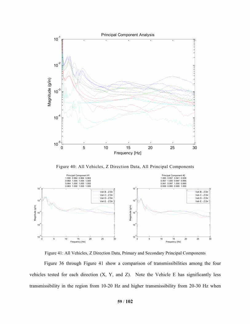
59 / 102
Figure 40: All Vehicles, Z Direction Data, All Principal Components
Figure 41: All Vehicles, Z Direction Data, Primary and Secondary Principal Components
Figure 36 through Figure 41 show a comparison of transmissibilities among the four
vehicles tested for each direction (X, Y, and Z). Note the Vehicle E has significantly less
transmissibility in the region from 10-20 Hz and higher transmissibility from 20-30 Hz when
0 5 10 15 20 25 3010
-5
10-4
10-3
10-2
10-1
Principal Component Analysis
Frequency [Hz]
Magnitude (
g/in)
0 5 10 15 20 25 3010
-5
10-4
10-3
10-2
10-1
Frequency [Hz]
Magnitude (
g/in)
Principal Component #1
1.000 0.964 0.964 0.963
0.964 1.000 1.000 1.000
0.964 1.000 1.000 1.000
0.963 1.000 1.000 1.000
Veh B - Z Dir
Veh C - Z Dir
Veh D - Z Dir
Veh E - Z Dir
0 5 10 15 20 25 3010
-5
10-4
10-3
10-2
10-1
Frequency [Hz]
Magnitude (
g/in)
Principal Component #2
1.000 0.957 0.941 0.936
0.957 1.000 0.997 0.995
0.941 0.997 1.000 0.995
0.936 0.995 0.995 1.000
Veh B - Z Dir
Veh C - Z Dir
Veh D - Z Dir
Veh E - Z Dir

60 / 102
compared to the field of vehicles tested. Due to strapping limitations, no conclusion can be
drawn from the 20-30 Hz range. The fact that Vehicle E is the ‘best in class’ specimen suggests
that lower transmissibility in the 10-20 Hz frequency range may be an important metric to track
for future evaluations. It should be noted that these conclusions are only speculation and further
testing with a more significant sample size will be needed to evaluate their validity. As an
anecdotal piece of information, Vehicle E was the only vehicle tested that used screw fasteners to
fasten interior trim panels and components. All other vehicles primarily used plastic interference
fasteners, sometimes referred to as Christmas tree fasteners, for most of the attachment of
interior trim and components.
4.5.4 Structure Comparisons
One of the primary reasons to compare different vehicles is to determine overall structure
characteristics that affect some performance criteria (squeak and rattle performance, for
example) in order to clearly see that one vehicle is different from other similar vehicles. In this
case, the vehicles are clearly different and looking at individual measurements or modal
properties may not easily give global or overall (similar or dissimilar) structure characteristics. It
may already be apparent based upon the previous sections that comparing the principal value
curves rather than individual or group transmissibilities is easier and allows trend information to
more easily be identified.

61 / 102
Figure 42: All Vehicles, All Data, All Principal Components
Figure 43: All Vehicles, All Data, Primary and Secondary Principal Components
When comparing the entire sets of data (as seen in Figure 42, Figure 44 and Figure 43),
the trends regarding the lower transmissibility of Vehicle E from 10 – 20 Hz continue.
0 5 10 15 20 25 3010
-5
10-4
10-3
10-2
10-1
Principal Component Analysis
Frequency [Hz]
Magnitude (
g/in)
0 5 10 15 20 25 3010
-5
10-4
10-3
10-2
10-1
Frequency [Hz]
Magnitude (
g/in)
Principal Component #1
1.000 0.985 0.985 0.984
0.985 1.000 1.000 1.000
0.985 1.000 1.000 1.000
0.984 1.000 1.000 1.000
Veh B
Veh C
Veh D
Veh E
0 5 10 15 20 25 3010
-5
10-4
10-3
10-2
10-1
Frequency [Hz]
Magnitude (
g/in)
Principal Component #2
1.000 0.958 0.956 0.997
0.958 1.000 0.999 0.975
0.956 0.999 1.000 0.974
0.997 0.975 0.974 1.000
Veh B
Veh C
Veh D
Veh E

62 / 102
4.5.5 Structural Component/Sub-System Comparison
This case is similar to the previous case but is limited to a subset of the data in the region
of the dashboard of each vehicle. Again, clear differences can be seen in the trend of the data
with some vehicles.
Figure 44: All Vehicles, Dash SubSystem, All Principal Components
0 5 10 15 20 25 3010
-5
10-4
10-3
10-2
10-1
Principal Component Analysis
Frequency [Hz]
Magnitude (
g/in)

63 / 102
Figure 45: All Vehicles, Dash SubSystem, Primary and Secondary Principal Components
When comparing specific subsets of data (as seen in Figure 44 and Figure 45), the trends
regarding the lower transmissibility of Vehicle E from 10 – 20 Hz continue.
0 5 10 15 20 25 3010
-5
10-4
10-3
10-2
10-1
Frequency [Hz]
Magnitude (
g/in)
Principal Component #1
1.000 1.000 1.000 1.000
1.000 1.000 1.000 1.000
1.000 1.000 1.000 1.000
1.000 1.000 1.000 1.000
Veh B
Veh C
Veh D
Veh E
0 5 10 15 20 25 3010
-5
10-4
10-3
10-2
10-1
Frequency [Hz]
Magnitude (
g/in)
Principal Component #2
1.000 0.945 0.951 0.989
0.945 1.000 0.999 0.980
0.951 0.999 1.000 0.983
0.989 0.980 0.983 1.000
Veh B
Veh C
Veh D
Veh E

64 / 102
Chapter 5. Conclusions and Future Work
5.1 Conclusions
The first half of this thesis has explored the background of transmissibility, the
development of the MIMO transmissibility function, and the application of the MIMO
transmissibility function on the UC-SDRL Four Axis Road Simulator. While this technique
looks promising, it is not conclusive given the relatively small sample size. Only one of each
vehicle type was available and little repeat testing was performed. Another challenge with this
technique is that, due to accessibility issues, sensor location was not always consistent vehicle to
vehicle. While this technique produced some useful results, it is tedious to make the
comparisons and identify trends with direct use of MIMO transmissibility.
The second half of this thesis has explored the general background, development and
application of Principal Component Analysis (PCA) to MIMO transmissibility measurements for
the specific case of a four axis road simulator and structural comparison studies. It has been
noted that techniques have been discovered and re-discovered over time as various analysis
problems have been encountered. Regardless of their original development, these various
ingenious decomposition techniques that reveal underlying linear contributors, all now share a
common numerical foundation in the singular value decomposition. Nonetheless, the various
intuitive physical interpretations of the MIMO transmissibility data matrix using PCA methods
are highly valuable contributions to the structural dynamics community. With their broad
applicability and ability to extract effective global trend information, the various PCA techniques
provide the analyst with robust numerical tools for making informed structure comparison
decisions.

65 / 102
5.2 Future Work
As mentioned previously, sensor locations were not always consistent from vehicle to
vehicle due to variations in geometry and accessibility. Future work could look to PCA
evaluation of group transmissibilities to help deal with these inconsistencies.
Principal components analysis of the various vehicles tested revealed a difference in
transmissibility in the 10-20 Hz region between the ‘best in class’ vehicle and the rest of the field
of specimens. Future testing with an expanded sample size could determine if this is a
meaningful metric with regards to identifying vehicles that will have “good” NVH
characteristics. This would include a more rigorous evaluation of the retention strap issue and
possible testing on a four axis road simulator with recessed actuators that does not require the use
of retention straps.

66 / 102
References
[1] A. Yee, Using Group Transmissibility Concepts to Compare Dissimilar Vehicle Platforms,
University of Cincinnati: MS Thesis, 2009.
[2] F. S. Tse, I. E. Morse and R. T. Hinkle, Mechanical Vibrations Theory and Applications, Boston,
MA: Allyn and Bacon, Inc., 1963.
[3] J. S. Bendat and A. G. Piersol, Random Data: Analysis and Measurement Procedures, New York:
John Wiley and Sons, Inc., 1971, p. 407.
[4] R. J. Allemang, Investigation of Some Multiple Input/Output Frequency Response Function
Experimental Modal Analysis Techniques, University of Cincinnati: PhD Dissertation, 1980, p. 359.
[5] I. Jolliffe, Principal Component Analysis, New York, NY: Springer-Verlag New York, Inc., 1986, p.
271.
[6] E. Deprettere, SVD and Signal Processing: Algorithms, Applications and Architectures, New York,
NY: Elsevier Science Publishing Company, Inc., 1988, p. 471.
[7] R. J. Allemang, A. W. Phillips and M. R. Allemang, "Application of Principal Compenent Analysis
Methods to Experimental Structural Dynamics," in Proceedings, International Modal Analysis
Conference, 2010.
[8] R. J. Allemang, Vibrations: Experimental Modal Analysis, August 2007 ed., University of
Cincinnati: Structural Dynamics Research Laboratory, 1990, pp. 5-8 - 5-30.
[9] R. W. Rost, Investigation of Mulitple Input Frequency Response Function Estimation Techniques for
Experimental Modal Analysis, University of Cincinnati: PhD Thesis, 1985, p. 237.
[10] J. Wilkinson, The Algebraic Eigenvalue Problem, Oxford: Oxford University Press, 1965, pp. 12-13.
[11] G. Strang, Linear Algebra and Its Applications, 3rd ed., San Diego, CA: Harcourt Brace Jovanovich
Publishers, 1988, p. 505.
[12] C. Lawson and R. Hanson, Solving Least Squares Problems, Englewood Cliffs, NJ: Prentice-Hall,
Inc., 1974, p. 340.
[13] L. Ljung, System Identification: Theory for the User, Englewood Cliffs, NJ: Prentice-Hall, Inc.,
1987, p. 519.
[14] A. Hyvarinen, J. Karhunen and E. Oja, Independent Component Analysis, New York, NY: John
Wiley & Sons,Inc., 2001.

67 / 102
[15] E. J. Jackson, User's Guide to Principal Components, Hoboken, NJ: John Wiley & Sons,Inc., 2003,
p. 569.
[16] R. J. Allemang, R. W. Rost and D. L. Brown, "Multiple Input Estimation of Frequency Response
Functions: Excitation Considerations," ASME Paper Number 83-DET-73, 1983.
[17] R. J. Allemang, D. L. Brown and R. W. Rost, "Multiple Input Estimation of Frequency Response,"
U.S. Air Force Report Number AFATL-TR-84-15, 1984.
[18] R. J. Allemang, D. L. Brown and R. W. Rost, "Measurement Techniques for Experimental Modal
Analysis," in Experimental Modal Analysis and Dynamic Component Synthesis, vol. 2, USAF
Technical Report, Contract Number F33615-83-C-3218, AFWAL-TR-87-3069, 1987.
[19] C. Shih, Y. Tsuei, R. Allemang and D. Brown, "Complex Mode Indication Function and Its
Application to Spatial Domain Parameter Estimation," Journal of Mechanical Systems and Signal
Processing, vol. 2, no. 4, pp. 367-372, 1988.
[20] C. Shih, Y. Tsuei, R. Allemang and D. Brown, "Complex Mode Indicator Function and its
Application to Spatial Domain Parameter Estimation," in Proceedings, 13th International Seminar
on Modal Analysis, Leuven, 1988.
[21] C. Shih, Y. Tsuei, R. Allemang and D. Brown, "Complex Mode Indication Function and its
Application to Spatial Domain Parameter Estimation," in Proceedings, International Modal Analysis
Conference, 1989.
[22] R. J. Allemang and L. D. Brown, "A Complete Review of the Complex Mode Indicator Function
(CMIF) with Applications," in Proceedings, International Conference on Noise and Vibration
Engineering (ISMA), Leuven, 2006.
[23] C. Pickrel, "Estimating the Rank of Measured Response Data Using SVD and Principal Response
Functions," in Proceedings of the Second International Conference on Structural Dynamics
Modeling, Test Analysis and Correlation DTA/NAFEMS, 1996.
[24] C. Pickrel, "Numerical Assessment of Test Data Using SVD," in Proceedings, International Modal
Analysis Conference, 1997, p. 1577.
[25] C. Pickrel, "Numerical Assessment of Test Data Using SVD," in Proceedings of SPIE, the
International Society for Optical Engineering, 1997.
[26] R. Mantrala, Squeak and Rattle Detection: A Comparative Experimental Data Analysis, University
of Cincinnati: MS Thesis, 2007.
[27] R. W. Clough and J. Penzien, Dynamics of Structures, 2nd Edition ed., B. J. Clark, Ed., New Yok,
New York: McGraw-Hll, 1993.
68 / 102
[28] M. Paz and W. Leigh, Structural Dynamics: Theory and Computation, 5th Edition ed., Boston,
Massachusetts: Kluwer Academic Publishers, 2004.
[29] R. J. Allemang, "The Modal Assurance Criterion (MAC): Twenty Years of Use and Abuse," Sound
and Vibration Magazine, vol. Vol. 37, no. No. 8, pp. 14-23, August 2003.
[30] W. Heylen and S. Lammens, "FRAC: A Consistent Way of Computing Frequency Response
Functions," in Proceedings, International Conference on Identification in Engineering, Swansea,
1996.
[31] R. D. Blevins, Formulas for Natural Frequency and Mode Shape, New York, NY: Van Nostrand
Reinhold, 1979.
[32] U. N. Godbole, Vehicle Road Test Simulation, University of Cincinnati: MS Thesis, 2005.
[33] M. Haroon, Nonlinear System Identification of a Tire-Vehicle Suspension System Using Response
Transmissibility, Purdue University: MS Thesis, 2003.

69 / 102
Appendix A. Vehicle A Instrumentation Setup
Channel Point Number Direction Data Type Model # S/N Calibration (V/EU) Comment EU
1 1 3 LVDT1 1 3.344 in
2 2 3 LVDT2 2 3.344
3 3 3 LVDT3 3 3.344
4 4 3 LVDT4 4 3.344
5 11 3 12 UT333M07 14217
6 12 3 12 UT333M07 15851
7 13 3 12 UT333M07 15540
8 14 3 12 UT333M07 16540
9 801 130A10/P10 0.025 Nominal Cal Pascal
10 802 130A10/P10 0.025 Nominal Cal
11 803 130A10/P10 0.025 Nominal Cal
12 804 130A10/P10 0.025 Nominal Cal
13 805 130A10/P10 0.025 Nominal Cal
14 806 130A10/P10 0.025 Nominal Cal
15 807 130A10/P10 0.025 Nominal Cal
16 808 130A10/P10 0.025 Nominal Cal
17 601 2 12 XT356B18x 59783 0.954 G-Unit
18 601 -1 12 XT356B18y 59783 0.915
19 601 3 12 XT356B18z 59783 0.830
20 602 2 12 XT356B18x 59797 0.929
21 602 -1 12 XT356B18y 59797 0.950
22 602 3 12 XT356B18z 59797 0.916
23 603 2 12 XT356B18x 59811 0.926
24 603 -1 12 XT356B18y 59811 0.876
25 603 3 12 XT356B18z 59811 0.988
26 604 2 12 XT356B18x 59781 0.940
27 604 -1 12 XT356B18y 59781 0.905
28 604 3 12 XT356B18z 59781 0.915
29 605 2 12 XT356B18x 59789 0.914
30 605 -1 12 XT356B18y 59789 0.959
31 605 3 12 XT356B18z 59789 0.954
32 606 2 12 XT356B18x 59803 0.978
33 606 -1 12 XT356B18y 59803 0.902
34 606 3 12 XT356B18z 59803 1.003
35 607 2 12 XT356B18x 59805 0.892
36 607 -1 12 XT356B18y 59805 0.966
37 607 3 12 XT356B18z 59805 0.974
38 608 2 12 XT356B18x 59785 0.861
39 608 -1 12 XT356B18y 59785 0.930
40 608 3 12 XT356B18z 59785 0.953

70 / 102
Channel Point Number Direction Data Type Model # S/N Calibration (V/EU) Comment EU
41 609 -2 12 XT356B18x 59799 0.929
42 609 -1 12 XT356B18y 59799 0.979
43 609 -3 12 XT356B18z 59799 0.941
44 610 -2 12 XT356B18x 59788 0.976
45 610 1 12 XT356B18y 59788 0.958
46 610 3 12 XT356B18z 59788 0.927
47 611 -2 12 T356B18x 16988 1.004
48 611 3 12 T356B18y 16988 1.024
49 611 -1 12 T356B18z 16988 1.039
50 612 -2 12 XT356B18x 59818 0.911
51 612 3 12 XT356B18y 59818 0.886
52 612 -1 12 XT356B18z 59818 0.887
53 613 -2 12 XT356B18x 59794 0.881
54 613 -1 12 XT356B18y 59794 0.957
55 613 -3 12 XT356B18z 59794 0.901
56 614 -2 12 XT356B18x 59776 0.943
57 614 -1 12 XT356B18y 59776 0.997
58 614 -3 12 XT356B18z 59776 0.961
59 615 2 12 XT356B18x 59772 0.931
60 615 -1 12 XT356B18y 59772 0.973
61 615 3 12 XT356B18z 59772 0.901
62 616 2 12 XT356B18x 59817 0.887
63 616 -1 12 XT356B18y 59817 0.853
64 616 3 12 XT356B18z 59817 0.919
65 617 2 12 XT356B18x 59820 0.964
66 617 -1 12 XT356B18y 59820 0.906
67 617 3 12 XT356B18z 59820 0.693
68 401 -1 12 XT356B18x 59807 0.932
69 401 3 12 XT356B18y 59807 0.931
70 401 2 12 XT356B18z 59807 0.922
71 402 -1 12 XT356B18x 59792 0.903
72 402 3 12 XT356B18y 59792 0.930
73 402 2 12 XT356B18z 59792 0.952
74 703 -1 12 XT356B18x 59802 0.923
75 703 2 12 XT356B18y 59802 0.945
76 703 -3 12 XT356B18z 59802 0.952
77 704 -1 12 XT356B18x 59806 0.960
78 704 2 12 XT356B18y 59806 0.970
79 704 -3 12 XT356B18z 59806 0.974
80 707 -1 12 XT356B18x 59810 0.946

71 / 102
Channel Point Number Direction Data Type Model # S/N Calibration (V/EU) Comment EU
81 707 2 12 XT356B18y 59810 0.925
82 707 -3 12 XT356B18z 59810 0.916
83 708 -1 12 XT356B18x 59812 0.893
84 708 2 12 XT356B18y 59812 0.942
85 708 -3 12 XT356B18z 59812 0.896
86 710 2 12 T356B18x 16975 1.000 Nominal Cal
87 710 -1 12 T356B18y 16975 1.000 Nominal Cal
88 710 3 12 T356B18z 16975 1.000 Nominal Cal
89 200 1 12 T356B18x 30815 1.047
90 200 3 12 T356B18y 30815 1.042
91 200 -2 12 T356B18z 30815 1.025
92 201 -1 12 T356B18x 29324 1.081
93 201 -2 12 T356B18y 29324 1.043
94 201 3 12 T356B18z 29324 1.094
95 202 -1 12 T356B18x 16979 1.000 Nominal Cal
96 202 -2 12 T356B18y 16979 1.000 Nominal Cal
97 202 3 12 T356B18z 16979 1.000 Nominal Cal
98 203 -1 12 XT356B18x 59771 0.962
99 203 -2 12 XT356B18y 59771 0.998
100 203 3 12 XT356B18z 59771 0.944
101 403 -1 12 T356B18x 16977 1.000 Nominal Cal
102 403 -2 12 T356B18y 16977 1.000 Nominal Cal
103 403 3 12 T356B18z 16977 1.000 Nominal Cal
104 503 2 12 T356B18x 16978 1.000 Nominal Cal
105 503 3 12 T356B18y 16978 1.000 Nominal Cal
106 503 1 12 T356B18z 16978 1.000 Nominal Cal
107 504 -2 12 XT356B18x 59770 0.980
108 504 1 12 XT356B18y 59770 0.908
109 504 3 12 XT356B18z 59770 0.930
110 507 -2 12 XT356B18x 59768 0.941
111 507 -3 12 XT356B18y 59768 0.939
112 507 1 12 XT356B18z 59768 0.951
113 505 -1 12 XT356B18x 59814 0.859
114 505 -2 12 XT356B18y 59814 0.926
115 505 3 12 XT356B18z 59814 0.954
116 301 -1 12 T356B18x 16968 1.000 Nominal Cal
117 301 -2 12 T356B18y 16968 1.000 Nominal Cal
118 301 3 12 T356B18z 16968 1.000 Nominal Cal
119 302 -1 12 XT356B18x 59816 0.946
120 302 -2 12 XT356B18y 59816 0.911

72 / 102
Channel Point Number Direction Data Type Model # S/N Calibration (V/EU) Comment EU
121 302 3 12 XT356B18z 59816 0.947
122 701 -1 12 T356B18x 16973 0.991
123 701 2 12 T356B18y 16973 1.055
124 701 -3 12 T356B18z 16973 0.988
125 702 -1 12 XT356B18x 59800 0.919
126 702 2 12 XT356B18y 59800 0.950
127 702 -3 12 XT356B18z 59800 0.966
128 705 -1 12 XT356B18x 59796 0.907
129 705 2 12 XT356B18y 59796 0.875
130 705 -3 12 XT356B18z 59796 0.837
131 706 -1 12 XT356B18x 59773 0.971
132 706 2 12 XT356B18y 59773 0.973
133 706 -3 12 XT356B18z 59773 0.909
134 709 2 12 T356B18x 16985 1.035
135 709 -1 12 T356B18y 16985 1.007
136 709 3 12 T356B18z 16985 1.043
137 100 1 12 T356B18x 16984 1.046
138 100 -3 12 T356B18y 16984 1.026
139 100 2 12 T356B18z 16984 1.019
140 101 -1 12 T356B18x 16976 1.063
141 101 -2 12 T356B18y 16976 1.019
142 101 3 12 T356B18z 16976 1.009
143 102 -1 12 T356B18x 29192 0.953
144 102 -2 12 T356B18y 29192 1.057
145 102 3 12 T356B18z 29192 0.996
146 103 -1 12 XT356B18x 59782 0.913
147 103 -2 12 XT356B18y 59782 0.942
148 103 3 12 XT356B18z 59782 0.964
149 303 -1 12 XT356B18x 59798 0.913
150 303 -2 12 XT356B18y 59798 0.936
151 303 3 12 XT356B18z 59798 0.957
152 501 -2 12 XT356B18x 59813 0.911
153 501 -3 12 XT356B18y 59813 0.888
154 501 1 12 XT356B18z 59813 0.924
155 502 -2 12 T356B18x 16986 1.000 Nominal Cal
156 502 -3 12 T356B18y 16986 1.000 Nominal Cal
157 502 1 12 T356B18z 16986 1.000 Nominal Cal
158 506 2 12 T356B18x 30816 0.946
159 506 3 12 T356B18y 30816 0.911
160 506 1 12 T356B18z 30816 0.947

73 / 102
Appendix B. Vehicle B Instrumentation Setup
Channel Point Number Direction Data Type Model # S/N Calibration (V/EU) Comment EU
1 31 3 8 LVDT1 1 3.344 in
2 32 3 8 LVDT2 2 3.344 in
3 33 3 8 LVDT3 3 3.344 in
4 34 3 8 LVDT4 4 3.344 in
5 101 1 12 XT356B18x 59803 0.9780 G
6 101 2 12 XT356B18y 59803 0.9020 G
7 101 3 12 XT356B18z 59803 1.0030 G
8 102 1 12 XT356B18x 59789 0.9140 G
9 102 2 12 XT356B18y 59789 0.9590 Pascal
10 102 3 12 XT356B18z 59789 0.9540 Pascal
11 103 1 12 XT356B18x 59783 0.9540 Pascal
12 103 2 12 XT356B18y 59783 0.9150 Pascal
13 103 3 12 XT356B18z 59783 0.8300 Pascal
14 104 1 12 XT356B18x 59768 0.9410 Pascal
15 104 2 12 XT356B18y 59768 0.9390 Pascal
16 104 3 12 XT356B18z 59768 0.9510 Pascal
17 105 1 12 XT356B18x 59813 0.9110 G
18 105 2 12 XT356B18y 59813 0.8880 G
19 105 3 12 XT356B18z 59813 0.9240 G
20 501 2 12 XT356B18x 59771 0.9620 G
21 501 3 12 XT356B18y 59771 0.9980 G
22 501 1 12 XT356B18z 59771 0.9440 G
23 502 2 12 T356B18x 16985 1.0350 G
24 502 3 12 T356B18y 16985 1.0070 G
25 502 1 12 T356B18z 16985 1.0430 G
26 503 2 12 XT356B18x 59799 0.9290 G
27 503 3 12 XT356B18y 59799 0.9790 G
28 503 1 12 XT356B18z 59799 0.9410 G
29 504 2 12 T356B18x 16975 1.0000 Nominal G
30 504 3 12 T356B18y 16975 1.0000 Nominal G
31 504 1 12 T356B18z 16975 1.0000 Nominal G
32 505 2 12 T356B18x 16978 1.0000 Nominal G
33 505 3 12 T356B18y 16978 1.0000 Nominal G
34 505 1 12 T356B18z 16978 1.0000 Nominal G
35 506 2 12 XT356B18x 59773 0.9710 G
36 506 3 12 XT356B18y 59773 0.9730 G
37 506 1 12 XT356B18z 59773 0.9090 G
38 507 -1 12 XT356B18x 59810 0.9460 G
39 507 2 12 XT356B18y 59810 0.9250 G
40 507 -3 12 XT356B18z 59810 0.9160 G

74 / 102
Channel Point Number Direction Data Type Model # S/N Calibration (V/EU) Comment EU
41 508 3 12 XT356B18x 59787 0.928 G
42 508 1 12 XT356B18y 59787 0.932 G
43 508 2 12 XT356B18z 59787 0.99 G
44 509 -1 12 XT356B18x 59775 0.9410 G
45 509 2 12 XT356B18y 59775 0.9900 G
46 509 -3 12 XT356B18z 59775 0.9240 G
47 510 1 12 T356B18x 29192 0.9530 G
48 510 2 12 T356B18y 29192 1.0570 G
49 510 3 12 T356B18z 29192 0.9960 G
50 201 1 12 XT356B18x 59806 0.9600 G
51 201 -2 12 XT356B18y 59806 0.9700 G
52 201 -3 12 XT356B18z 59806 0.9740 G
53 202 1 12 XT356B18x 59788 0.9760 G
54 202 -2 12 XT356B18y 59788 0.9580 G
55 202 -3 12 XT356B18z 59788 0.9270 G
56 203 1 12 XT356B18x 59811 0.9260 G
57 203 2 12 XT356B18y 59811 0.8760 G
58 203 3 12 XT356B18z 59811 0.9880 G
59 204 1 12 T356B18x 16977 1.0000 Nominal G
60 204 2 12 T356B18y 16977 1.0000 Nominal G
61 204 3 12 T356B18z 16977 1.0000 Nominal G
62 205 1 12 XT356B18x 59797 0.9290 G
63 205 2 12 XT356B18y 59797 0.9500 G
64 205 3 12 XT356B18z 59797 0.9160 G
65 601 1 12 T356B18x 30809 1.061 G
66 601 -2 12 T356B18y 30809 0.999 G
67 601 -3 12 T356B18z 30809 1.057 G
68 602 1 12 XT356B18x 59816 0.9460 G
69 602 -2 12 XT356B18y 59816 0.9110 G
70 602 -3 12 XT356B18z 59816 0.9470 G
71 603 1 12 XT356B18x 59794 0.8810 G
72 603 -2 12 XT356B18y 59794 0.9570 G
73 603 -3 12 XT356B18z 59794 0.9010 G
74 604 1 12 XT356B18x 59798 0.9130 G
75 604 -2 12 XT356B18y 59798 0.9360 G
76 604 -3 12 XT356B18z 59798 0.9570 G
77 605 1 12 XT356B18x 59800 0.9190 G
78 605 -2 12 XT356B18y 59800 0.9500 G
79 605 -3 12 XT356B18z 59800 0.9660 G
80 606 1 12 XT356B18x 59790 0.951 G

75 / 102
Channel Point Number Direction Data Type Model # S/N Calibration (V/EU) Comment EU
81 606 -2 12 XT356B18y 59790 0.91 G
82 606 -3 12 XT356B18z 59790 0.921 G
83 607 1 12 T356B18x 30816 0.9460 G
84 607 2 12 T356B18y 30816 0.9110 G
85 607 3 12 T356B18z 30816 0.9470 G
86 608 3 12 T356B18x 16976 1.0630 G
87 608 -1 12 T356B18y 16976 1.0190 G
88 608 -2 12 T356B18z 16976 1.0090 G
89 609 3 12 XT356B18x 59818 0.9110 G
90 609 2 12 XT356B18y 59818 0.8860 G
91 609 -1 12 XT356B18z 59818 0.8870 G
92 610 3 12 XT356B18x 59781 0.9400 G
93 610 2 12 XT356B18y 59781 0.9050 G
94 610 -1 12 XT356B18z 59781 0.9150 G
95 711 -1 12 XT356B18x 59817 0.8870 G
96 711 2 12 XT356B18y 59817 0.8530 G
97 711 -3 12 XT356B18z 59817 0.9190 G
98 712 -1 12 XT356B18x 59805 0.8920 G
99 712 2 12 XT356B18y 59805 0.9660 G
100 712 -3 12 XT356B18z 59805 0.9740 G
101 713 -1 12 T356B18x 16988 1.0040 G
102 713 2 12 T356B18y 16988 1.0240 G
103 713 -3 12 T356B18z 16988 1.0390 G
104 714 -1 12 XT356B18x 59812 0.8930 G
105 714 2 12 XT356B18y 59812 0.9420 G
106 714 -3 12 XT356B18z 59812 0.8960 G
107 721 -1 12 XT356B18x 59814 0.8590 G
108 721 2 12 XT356B18y 59814 0.9260 G
109 721 -3 12 XT356B18z 59814 0.9540 G
110 722 -1 12 XT356B18x 59776 0.9430 G
111 722 2 12 XT356B18y 59776 0.9970 G
112 722 -3 12 XT356B18z 59776 0.9610 G
113 723 -1 12 XT356B18x 59802 0.9230 G
114 723 2 12 XT356B18y 59802 0.9450 G
115 723 -3 12 XT356B18z 59802 0.9520 G
116 724 -1 12 XT356B18x 59820 0.9640 G
117 724 2 12 XT356B18y 59820 0.9060 G
118 724 -3 12 XT356B18z 59820 0.6930 G
119 001 3 12 UT333M07 15851 1 Nominal G
120 002 3 12 UT333M08 15540 1 Nominal G

76 / 102
Channel Point Number Direction Data Type Model # S/N Calibration (V/EU) Comment EU
121 003 3 12 UT333M09 14217 1 Nominal G
122 004 3 12 UT333M10 16540 1 Nominal G
123 011 3 12 UT333M11 14625 1 Nominal G
124 012 3 12 UT333M12 18529 1 Nominal G
125 013 3 12 UT333M13 18528 1 Nominal G
126 014 3 12 UT333M14 15845 1 Nominal G
127 811 2 21 130A10/P10 2624/2658 0.01761 G
128 812 -2 21 130A10/P10 5803/5728 0.03333 G
129 813 1 21 130A10/P10 2620/2665 0.01997 G
130 814 1 21 130A10/P10 3982/2668 0.02166 G
131 821 2 21 130A10/P10 2642/2673 0.02149 G
132 822 -2 21 130A10/P10 2640/2662 0.02007 G
133 823 1 21 130A10/P10 2628/2664 0.02138 G
134 824 1 21 130A10/P10 2631/2655 0.02031 G
135 901 1 12 XT356B18x 59770 0.9800 G
136 901 2 12 XT356B18y 59770 0.9080 G
137 901 3 12 XT356B18z 59770 0.9300 G
138 902 1 12 XT356B18x 59792 0.9030 G
139 902 2 12 XT356B18y 59792 0.9300 G
140 902 3 12 XT356B18z 59792 0.9520 G
141 903 1 12 XT356B18x 59769 0.9920 G
142 903 2 12 XT356B18y 59769 0.9210 G
143 903 3 12 XT356B18z 59769 0.9190 G
144 904 1 12 XT356B18x 59791 0.907 G
145 904 2 12 XT356B18y 59791 0.959 G
146 904 3 12 XT356B18z 59791 0.915 G
147 905 3 12 T356B18x 16973 0.9910 G
148 905 2 12 T356B18y 16973 1.0550 G
149 905 -1 12 T356B18z 16973 0.9880 G
150 906 3 12 T356B18x 16984 1.0460 G
151 906 2 12 T356B18y 16984 1.0260 G
152 906 -1 12 T356B18z 16984 1.0190 G
153 907 3 12 T356B18x 16979 1.0000 Nominal G
154 907 2 12 T356B18y 16979 1.0000 Nominal G
155 907 -1 12 T356B18z 16979 1.0000 Nominal G
156 908 3 12 XT356B18x 59785 0.8610 G
157 908 2 12 XT356B18y 59785 0.9300 G
158 908 -1 12 XT356B18z 59785 0.9530 G
159 1 1 1 1 1 1
160 1 1 1 1 1 1

77 / 102
Appendix C. Vehicle C Instrumentation Setup
Channel Point Number Direction Data Type Model # S/N Calibration (V/EU) Comment EU
1 1 3 8 LVDT1 1 3.344 in
2 2 3 8 LVDT2 2 3.344 in
3 3 3 8 LVDT3 3 3.344 in
4 4 3 8 LVDT4 4 3.344 in
5 101 1 12 XT356B18x 59771 0.9620 G
6 101 -3 12 XT356B18y 59771 0.9980 G
7 101 2 12 XT356B18z 59771 0.9440 G
8 102 1 12 XT356B18x 59776 0.9430 G
9 102 -3 12 XT356B18y 59776 0.9970 G
10 102 2 12 XT356B18z 59776 0.9610 G
11 103 1 12 XT356B18x 59785 0.8610 G
12 103 2 12 XT356B18y 59785 0.9300 G
13 103 3 12 XT356B18z 59785 0.9530 G
14 104 1 12 XT356B18x 59798 0.9130 G
15 104 2 12 XT356B18y 59798 0.9360 G
16 104 3 12 XT356B18z 59798 0.9570 G
17 105 1 12 XT356B18x 59768 0.9410 G
18 105 2 12 XT356B18y 59768 0.9390 G
19 105 3 12 XT356B18z 59768 0.9510 G
20 501 2 12 XT356B18x 59800 0.9190 G
21 501 3 12 XT356B18y 59800 0.9500 G
22 501 1 12 XT356B18z 59800 0.9660 G
23 502 2 12 XT356B18x 59817 0.8870 G
24 502 3 12 XT356B18y 59817 0.8530 G
25 502 1 12 XT356B18z 59817 0.9190 G
26 503 2 12 XT356B18x 59820 0.9640 G
27 503 3 12 XT356B18y 59820 0.9060 G
28 503 1 12 XT356B18z 59820 0.6930 G
29 504 2 12 XT356B18x 59791 0.907 G
30 504 3 12 XT356B18y 59791 0.959 G
31 504 1 12 XT356B18z 59791 0.915 G
32 505 1 12 XT356B18x 59802 0.9230 G
33 505 2 12 XT356B18y 59802 0.9450 G
34 505 3 12 XT356B18z 59802 0.9520 G
35 506 1 12 XT356B18x 59812 0.8930 G
36 506 2 12 XT356B18y 59812 0.9420 G
37 506 3 12 XT356B18z 59812 0.8960 G
38 507 3 12 XT356B18x 59810 0.9460 G
39 507 1 12 XT356B18y 59810 0.9250 G
40 507 2 12 XT356B18z 59810 0.9160 G
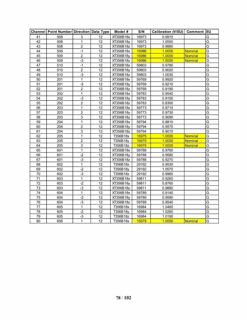
78 / 102
Channel Point Number Direction Data Type Model # S/N Calibration (V/EU) Comment EU
41 508 3 12 XT356B18x 16973 0.9910 G
42 508 1 12 XT356B18y 16973 1.0550 G
43 508 2 12 XT356B18z 16973 0.9880 G
44 509 -1 12 XT356B18x 16986 1.0000 Nominal G
45 509 2 12 XT356B18y 16986 1.0000 Nominal G
46 509 -3 12 XT356B18z 16986 1.0000 Nominal G
47 510 -1 12 XT356B18x 59803 0.9780 G
48 510 2 12 XT356B18y 59803 0.9020 G
49 510 -3 12 XT356B18z 59803 1.0030 G
50 201 1 12 XT356B18x 59769 0.9920 G
51 201 -3 12 XT356B18y 59769 0.9210 G
52 201 2 12 XT356B18z 59769 0.9190 G
53 202 1 12 XT356B18x 59783 0.9540 G
54 202 -3 12 XT356B18y 59783 0.9150 G
55 202 2 12 XT356B18z 59783 0.8300 G
56 203 1 12 XT356B18x 59773 0.9710 G
57 203 2 12 XT356B18y 59773 0.9730 G
58 203 3 12 XT356B18z 59773 0.9090 G
59 204 1 12 XT356B18x 59794 0.8810 G
60 204 2 12 XT356B18y 59794 0.9570 G
61 204 3 12 XT356B18z 59794 0.9010 G
62 205 1 12 T356B18x 16975 1.0000 Nominal G
63 205 2 12 T356B18y 16975 1.0000 Nominal G
64 205 3 12 T356B18z 16975 1.0000 Nominal G
65 601 1 12 XT356B18x 59788 0.9760 G
66 601 -2 12 XT356B18y 59788 0.9580 G
67 601 -3 12 XT356B18z 59788 0.9270 G
68 602 1 12 T356B18x 29192 0.9530 G
69 602 -2 12 T356B18y 29192 1.0570 G
70 602 -3 12 T356B18z 29192 0.9960 G
71 603 1 12 XT356B18x 59811 0.9260 G
72 603 -2 12 XT356B18y 59811 0.8760 G
73 603 -3 12 XT356B18z 59811 0.9880 G
74 604 1 12 XT356B18x 59789 0.9140 G
75 604 -2 12 XT356B18y 59789 0.9590 G
76 604 -3 12 XT356B18z 59789 0.9540 G
77 605 1 12 T356B18x 16984 1.0460 G
78 605 -2 12 T356B18y 16984 1.0260 G
79 605 -3 12 T356B18z 16984 1.0190 G
80 606 1 12 T356B18x 16979 1.0000 Nominal G

79 / 102
Channel Point Number Direction Data Type Model # S/N Calibration (V/EU) Comment EU
81 606 -2 12 T356B18y 16979 1.0000 Nominal G
82 606 -3 12 T356B18z 16979 1.0000 Nominal G
83 607 3 12 XT356B18x 59806 0.9600 G
84 607 2 12 XT356B18y 59806 0.9700 G
85 607 -1 12 XT356B18z 59806 0.9740 G
86 608 3 12 XT356B18x 59814 0.8590 G
87 608 2 12 XT356B18y 59814 0.9260 G
88 608 -1 12 XT356B18z 59814 0.9540 G
89 609 3 12 T356B18x 16977 1.0000 Nominal G
90 609 2 12 T356B18y 16977 1.0000 Nominal G
91 609 -1 12 T356B18z 16977 1.0000 Nominal G
92 711 -1 12 XT356B18x 59775 0.9410 G
93 711 2 12 XT356B18y 59775 0.9900 G
94 711 -3 12 XT356B18z 59775 0.9240 G
95 712 -1 12 XT356B18x 59813 0.9110 G
96 712 2 12 XT356B18y 59813 0.8880 G
97 712 -3 12 XT356B18z 59813 0.9240 G
98 713 -1 12 XT356B18x 59790 0.951 G
99 713 2 12 XT356B18y 59790 0.91 G
100 713 -3 12 XT356B18z 59790 0.921 G
101 714 -1 12 XT356B18x 59781 0.9400 G
102 714 2 12 XT356B18y 59781 0.9050 G
103 714 -3 12 XT356B18z 59781 0.9150 G
104 721 -1 12 T356B18x 30809 1.061 G
105 721 2 12 T356B18y 30809 0.999 G
106 721 -3 12 T356B18z 30809 1.057 G
107 722 -1 12 XT356B18x 59787 0.928 G
108 722 2 12 XT356B18y 59787 0.932 G
109 722 -3 12 XT356B18z 59787 0.99 G
110 723 -1 12 T356B18x 16988 1.0040 G
111 723 2 12 T356B18y 16988 1.0240 G
112 723 -3 12 T356B18z 16988 1.0390 G
113 724 -1 12 T356B18x 16985 1.0350 G
114 724 2 12 T356B18y 16985 1.0070 G
115 724 -3 12 T356B18z 16985 1.0430 G
116 11 3 12 UT333M07 18528 1.0000 Nominal Cal G
117 12 3 12 UT333M07 15845 1.0000 Nominal Cal G
118 13 3 12 UT333M07 14625 1.0000 Nominal Cal G
119 14 3 12 UT333M07 18529 1.0000 Nominal Cal G
120 21 3 12 UT333M07 15540 1.0000 Nominal Cal G

80 / 102
Channel Point Number Direction Data Type Model # S/N Calibration (V/EU) Comment EU
121 22 3 12 UT333M07 16540 1.0000 Nominal Cal G
122 23 3 12 UT333M07 15851 1.0000 Nominal Cal G
123 24 3 12 UT333M07 14217 1.0000 Nominal Cal G
124 811 2 21 130A10/P10 5803/5728 0.03333 Pascal
125 812 -2 21 130A10/P10 2628/2664 0.02138 Pascal
126 813 1 21 130A10/P10 2620/2665 0.01997 Pascal
127 814 1 21 130A10/P10 2624/2658 0.01761 Pascal
128 821 2 21 130A10/P10 2642/2673 0.02149 Pascal
129 822 -2 21 130A10/P10 3982/2668 0.02166 Pascal
130 823 1 21 130A10/P10 2640/2662 0.02007 Pascal
131 824 1 21 130A10/P10 2631/2655 0.02031 Pascal
132 901 1 12 T356B18x 30816 0.9460 G
133 901 2 12 T356B18y 30816 0.9110 G
134 901 3 12 T356B18z 30816 0.9470 G
135 902 1 12 T356B18x 16976 1.0630 G
136 902 2 12 T356B18y 16976 1.0190 G
137 902 3 12 T356B18z 16976 1.0090 G
138 903 1 12 XT356B18x 59818 0.9110 G
139 903 2 12 XT356B18y 59818 0.8860 G
140 903 3 12 XT356B18z 59818 0.8870 G
141 904 1 12 XT356B18x 59805 0.8920 G
142 904 2 12 XT356B18y 59805 0.9660 G
143 904 3 12 XT356B18z 59805 0.9740 G
144 905 3 12 XT356B18x 59797 0.9290 G
145 905 2 12 XT356B18y 59797 0.9500 G
146 905 -1 12 XT356B18z 59797 0.9160 G
147 906 3 12 XT356B18x 59792 0.9030 G
148 906 2 12 XT356B18y 59792 0.9300 G
149 906 -1 12 XT356B18z 59792 0.9520 G
150 907 3 12 XT356B18x 59770 0.9800 G
151 907 2 12 XT356B18y 59770 0.9080 G
152 907 -1 12 XT356B18z 59770 0.9300 G
153 908 3 12 XT356B18x 59799 0.9290 G
154 908 2 12 XT356B18y 59799 0.9790 G
155 908 -1 12 XT356B18z 59799 0.9410 G
156 909 1 12 T356B18x 16978 1.0000 Nominal G
157 909 2 12 T356B18y 16978 1.0000 Nominal G
158 909 3 12 T356B18z 16978 1.0000 Nominal G

81 / 102
Appendix D. Vehicle D Instrumentation Setup
Channel Point Number Direction Data Type Model # S/N Calibration (V/EU) Comment EU
1 1 3 8 LVDT1 1 3.344 in
2 2 3 8 LVDT2 2 3.344 in
3 3 3 8 LVDT3 3 3.344 in
4 4 3 8 LVDT4 4 3.344 in
5 101 1 12 XT356B18x 59805 0.8920 G
6 101 2 12 XT356B18y 59805 0.9660 G
7 101 3 12 XT356B18z 59805 0.9740 G
8 102 1 12 XT356B18x 59810 0.9460 G
9 102 2 12 XT356B18y 59810 0.9250 G
10 102 3 12 XT356B18z 59810 0.9160 G
11 103 1 12 XT356B18x 59775 0.9410 G
12 103 2 12 XT356B18y 59775 0.9900 G
13 103 3 12 XT356B18z 59775 0.9240 G
14 104 1 12 XT356B18x 59811 0.9260 G
15 104 2 12 XT356B18y 59811 0.8760 G
16 104 3 12 XT356B18z 59811 0.9880 G
17 105 1 12 T356B18x 29192 0.9530 G
18 105 2 12 T356B18y 29192 1.0570 G
19 105 3 12 T356B18z 29192 0.9960 G
20 501 -2 12 XT356B18x 59817 0.8870 G
21 501 -3 12 XT356B18y 59817 0.8530 G
22 501 1 12 XT356B18z 59817 0.9190 G
23 502 -2 12 T356B18x 16978 1.0000 G
24 502 -3 12 T356B18y 16978 1.0000 G
25 502 1 12 T356B18z 16978 1.0000 G
26 503 2 12 XT356B18x 59812 0.8930 G
27 503 3 12 XT356B18y 59812 0.9420 G
28 503 1 12 XT356B18z 59812 0.8960 G
29 504 2 12 XT356B18x 59783 0.9540 G
30 504 3 12 XT356B18y 59783 0.9150 G
31 504 1 12 XT356B18z 59783 0.8300 G
32 303 -1 12 XT356B18x 59820 0.9640 G
33 303 -2 12 XT356B18y 59820 0.9060 G
34 303 3 12 XT356B18z 59820 0.6930 G
35 403 1 12 XT356B18x 59798 0.9130 G
36 403 2 12 XT356B18y 59798 0.9360 G
37 403 3 12 XT356B18z 59798 0.9570 G
38 401 3 12 XT356B18x 59788 0.9760 G
39 401 1 12 XT356B18y 59788 0.9580 G
40 401 2 12 XT356B18z 59788 0.9270 G

82 / 102
Channel Point Number Direction Data Type Model # S/N Calibration (V/EU) Comment EU
41 301 3 12 XT356B18x 59806 0.9600 G
42 301 -1 12 XT356B18y 59806 0.9700 G
43 301 -2 12 XT356B18z 59806 0.9740 G
44 302 3 12 T356B18x 16977 1.0000 G
45 302 -1 12 T356B18y 16977 1.0000 G
46 302 -2 12 T356B18z 16977 1.0000 G
47 402 3 12 XT356B18x 59814 0.8590 G
48 402 1 12 XT356B18y 59814 0.9260 G
49 402 2 12 XT356B18z 59814 0.9540 G
50 201 1 12 XT356B18x 59802 0.9230 G
51 201 -2 12 XT356B18y 59802 0.9450 G
52 201 -3 12 XT356B18z 59802 0.9520 G
53 202 1 12 XT356B18x 59799 0.9290 G
54 202 -2 12 XT356B18y 59799 0.9790 G
55 202 -3 12 XT356B18z 59799 0.9410 G
56 203 1 12 XT356B18x 59785 0.8610 G
57 203 2 12 XT356B18y 59785 0.9300 G
58 203 3 12 XT356B18z 59785 0.9530 G
59 204 1 12 T356B18x 30816 0.9460 G
60 204 2 12 T356B18y 30816 0.9110 G
61 204 3 12 T356B18z 30816 0.9470 G
62 205 1 12 T356B18x 16975 1.0000 G
63 205 2 12 T356B18y 16975 1.0000 G
64 205 3 12 T356B18z 16975 1.0000 G
65 601 1 12 XT356B18x 16973 0.9910 G
66 601 -2 12 XT356B18y 16973 1.0550 G
67 601 -3 12 XT356B18z 16973 0.9880 G
68 602 -1 12 XT356B18x 16986 1.0000 G
69 602 -2 12 XT356B18y 16986 1.0000 G
70 602 3 12 XT356B18z 16986 1.0000 G
71 603 1 12 XT356B18x 59794 0.8810 G
72 603 2 12 XT356B18y 59794 0.9570 G
73 603 3 12 XT356B18z 59794 0.9010 G
74 604 1 12 T356B18x 16976 1.0630 G
75 604 2 12 T356B18y 16976 1.0190 G
76 604 3 12 T356B18z 16976 1.0090 G
77 605 1 12 T356B18x 16984 1.0460 G
78 605 -2 12 T356B18y 16984 1.0260 G
79 605 -3 12 T356B18z 16984 1.0190 G
80 606 1 12 XT356B18x 59770 0.9800 G

83 / 102
Channel Point Number Direction Data Type Model # S/N Calibration (V/EU) Comment EU
81 606 -2 12 XT356B18y 59770 0.9080 G
82 606 -3 12 XT356B18z 59770 0.9300 G
83 607 -2 12 XT356B18x 29324 1.0000 G
84 607 3 12 XT356B18y 29324 1.0000 G
85 607 -1 12 XT356B18z 29324 1.0000 G
86 608 3 12 T356B18x 59786 1.000 G
87 608 2 12 T356B18y 59786 1.000 G
88 608 -1 12 T356B18z 59786 1.000 G
89 609 1 12 T356B18x 16988 1.0040 G
90 609 3 12 T356B18y 16988 1.0240 G
91 609 -2 12 T356B18z 16988 1.0390 G
92 711 -1 12 XT356B18x 59790 0.951 G
93 711 2 12 XT356B18y 59790 0.91 G
94 711 -3 12 XT356B18z 59790 0.921 G
95 712 -1 12 XT356B18x 59800 0.9190 G
96 712 2 12 XT356B18y 59800 0.9500 G
97 712 -3 12 XT356B18z 59800 0.9660 G
98 713 -1 12 XT356B18x 59813 0.9110 G
99 713 2 12 XT356B18y 59813 0.8880 G
100 713 -3 12 XT356B18z 59813 0.9240 G
101 714 -1 12 XT356B18x 59797 0.9290 G
102 714 2 12 XT356B18y 59797 0.9500 G
103 714 -3 12 XT356B18z 59797 0.9160 G
104 721 -1 12 XT356B18x 59781 0.9400 G
105 721 2 12 XT356B18y 59781 0.9050 G
106 721 -3 12 XT356B18z 59781 0.9150 G
107 722 -1 12 T356B18x 16979 1.0000 G
108 722 2 12 T356B18y 16979 1.0000 G
109 722 -3 12 T356B18z 16979 1.0000 G
110 723 -1 12 XT356B18x 59787 0.928 G
111 723 2 12 XT356B18y 59787 0.932 G
112 723 -3 12 XT356B18z 59787 0.99 G
113 724 -1 12 XT356B18x 59792 0.9030 G
114 724 2 12 XT356B18y 59792 0.9300 G
115 724 -3 12 XT356B18z 59792 0.9520 G
116 11 1 12 UT333M07 14625 1.0000 G
117 12 1 12 UT333M07 18529 1.0000 G
118 13 1 12 UT333M07 18528 1.0000 G
119 14 1 12 UT333M07 15845 1.0000 G
120 21 1 12 UT333M07 14217 1.0000 G

84 / 102
Channel Point Number Direction Data Type Model # S/N Calibration (V/EU) Comment EU
121 22 1 12 UT333M07 15851 1.0000 G
122 23 1 12 UT333M07 15632 1.0000 G
123 24 1 12 UT333M07 15540 1.0000 G
124 811 2 21 130A10/P10 2628/2664 0.02138 Pascal
125 812 -2 21 130A10/P10 3982/2668 0.02166 Pascal
126 813 1 21 130A10/P10 2624/2658 0.01761 Pascal
127 814 1 21 130A10/P10 2620/2665 0.01997 Pascal
128 821 2 21 130A10/P10 2631/2655 0.02031 Pascal
129 822 -2 21 130A10/P10 2640/2662 0.02007 Pascal
130 823 1 21 130A10/P10 5803/5728 0.03333 Pascal
131 824 1 21 130A10/P10 2642/2673 0.02149 Pascal
132 901 1 12 XT356B18x 59789 0.9140 G
133 901 2 12 XT356B18y 59789 0.9590 G
134 901 3 12 XT356B18z 59789 0.9540 G
135 902 1 12 XT356B18x 59818 0.9110 G
136 902 2 12 XT356B18y 59818 0.8860 G
137 902 3 12 XT356B18z 59818 0.8870 G
138 903 1 12 XT356B18x 59769 0.9920 G
139 903 2 12 XT356B18y 59769 0.9210 G
140 903 3 12 XT356B18z 59769 0.9190 G
141 904 1 12 XT356B18x 59773 0.9710 G
142 904 2 12 XT356B18y 59773 0.9730 G
143 904 3 12 XT356B18z 59773 0.9090 G
144 905 3 12 XT356B18x 59768 0.9410 G
145 905 2 12 XT356B18y 59768 0.9390 G
146 905 -1 12 XT356B18z 59768 0.9510 G
147 906 3 12 XT356B18x 59803 0.9780 G
148 906 2 12 XT356B18y 59803 0.9020 G
149 906 -1 12 XT356B18z 59803 1.0030 G
150 907 3 12 XT356B18x 59791 0.907 G
151 907 2 12 XT356B18y 59791 0.959 G
152 907 -1 12 XT356B18z 59791 0.915 G
153 908 3 12 XT356B18x 59776 0.9430 G
154 908 2 12 XT356B18y 59776 0.9970 G
155 908 -1 12 XT356B18z 59776 0.9610 G
156 909 1 12 T356B18x 16985 1.0350 G
157 909 2 12 T356B18y 16985 1.0070 G
158 909 3 12 T356B18z 16985 1.0430 G
159 1 1 1 1 1 1
160 1 1 1 1 1 1

85 / 102
Appendix E. Vehicle E Instrumentation Setup
Channel Point Number Direction Data Type Model # S/N Calibration (V/EU) Comment EU
1 1 3 8 LVDT1 1 3.344 in
2 2 3 8 LVDT2 2 3.344 in
3 3 3 8 LVDT3 3 3.344 in
4 4 3 8 LVDT4 4 3.344 in
5 101 1 12 XT356B18x 16979 1.0000 G
6 101 2 12 XT356B18y 16979 1.0000 G
7 101 3 12 XT356B18z 16979 1.0000 G
8 102 1 12 XT356B18x 16976 1.0630 G
9 102 2 12 XT356B18y 16976 1.0190 G
10 102 3 12 XT356B18z 16976 1.0090 G
11 103 1 12 XT356B18x 59794 0.8810 G
12 103 2 12 XT356B18y 59794 0.9570 G
13 103 3 12 XT356B18z 59794 0.9010 G
14 104 1 12 XT356B18x 59820 0.9640 G
15 104 2 12 XT356B18y 59820 0.9060 G
16 104 3 12 XT356B18z 59820 0.6930 G
17 105 1 12 XT356B18x 30814 1.0080 G
18 105 2 12 XT356B18y 30814 0.9810 G
19 105 3 12 XT356B18z 30814 1.0740 G
20 501 -2 12 XT356B18x 59785 0.8610 G
21 501 -3 12 XT356B18y 59785 0.9300 G
22 501 1 12 XT356B18z 59785 0.9530 G
23 502 -2 12 XT356B18x 59797 0.9290 G
24 502 -3 12 XT356B18y 59797 0.9500 G
25 502 1 12 XT356B18z 59797 0.9160 G
26 503 2 12 XT356B18x 59792 0.9030 G
27 503 3 12 XT356B18y 59792 0.9300 G
28 503 1 12 XT356B18z 59792 0.9520 G
29 504 -2 12 XT356B18x 16975 1.0000 G
30 504 -3 12 XT356B18y 16975 1.0000 G
31 504 1 12 XT356B18z 16975 1.0000 G
32 303 -1 12 XT356B18x 30816 0.9460 G
33 303 -2 12 XT356B18y 30816 0.9110 G
34 303 3 12 XT356B18z 30816 0.9470 G
35 403 1 12 XT356B18x 59775 0.9410 G
36 403 2 12 XT356B18y 59775 0.9900 G
37 403 3 12 XT356B18z 59775 0.9240 G
38 401 -1 12 XT356B18x 59773 0.9710 G
39 401 -2 12 XT356B18y 59773 0.9730 G
40 401 3 12 XT356B18z 59773 0.9090 G

86 / 102
Channel Point Number Direction Data Type Model # S/N Calibration (V/EU) Comment EU
41 301 -1 12 XT356B18x 59789 0.9140 G
42 301 -3 12 XT356B18y 59789 0.9590 G
43 301 2 12 XT356B18z 59789 0.9540 G
44 302 -1 12 XT356B18x 16978 1.0000 G
45 302 2 12 XT356B18y 16978 1.0000 G
46 302 -3 12 XT356B18z 16978 1.0000 G
47 402 -1 12 XT356B18x 59781 0.9400 G
48 402 -2 12 XT356B18y 59781 0.9050 G
49 402 3 12 XT356B18z 59781 0.9150 G
50 201 1 12 XT356B18x 16986 1.0000 G
51 201 -2 12 XT356B18y 16986 1.0000 G
52 201 -3 12 XT356B18z 16986 1.0000 G
53 202 1 12 XT356B18x 59799 0.9290 G
54 202 -2 12 XT356B18y 59799 0.9790 G
55 202 -3 12 XT356B18z 59799 0.9410 G
56 203 1 12 XT356B18x 59770 0.9800 G
57 203 2 12 XT356B18y 59770 0.9080 G
58 203 3 12 XT356B18z 59770 0.9300 G
59 204 1 12 XT356B18x 59817 0.8870 G
60 204 2 12 XT356B18y 59817 0.8530 G
61 204 3 12 XT356B18z 59817 0.9190 G
62 205 1 12 XT356B18x 59803 0.9780 G
63 205 2 12 XT356B18y 59803 0.9020 G
64 205 3 12 XT356B18z 59803 1.0030 G
65 601 1 12 XT356B18x 59790 0.951 G
66 601 -2 12 XT356B18y 59790 0.91 G
67 601 -3 12 XT356B18z 59790 0.921 G
68 602 -1 12 XT356B18x 59810 0.9460 G
69 602 -2 12 XT356B18y 59810 0.9250 G
70 602 3 12 XT356B18z 59810 0.9160 G
71 603 1 12 XT356B18x 29324 1.0000 G
72 603 -2 12 XT356B18y 29324 1.0000 G
73 603 -3 12 XT356B18z 29324 1.0000 G
74 505 -1 12 XT356B18x 59786 1.000 G
75 505 2 12 XT356B18y 59786 1.000 G
76 505 -3 12 XT356B18z 59786 1.000 G
77 605 2 12 XT356B18x 59769 0.9920 G
78 605 -3 12 XT356B18y 59769 0.9210 G
79 605 -1 12 XT356B18z 59769 0.9190 G
80 606 3 12 XT356B18x 16985 1.0350 G

87 / 102
Channel Point Number Direction Data Type Model # S/N Calibration (V/EU) Comment EU
81 606 2 12 XT356B18y 16985 1.0070 G
82 606 -1 12 XT356B18z 16985 1.0430 G
83 607 1 12 XT356B18x 59807 0.9320 G
84 607 -2 12 XT356B18y 59807 0.9310 G
85 607 -3 12 XT356B18z 59807 0.9220 G
86 608 1 12 XT356B18x 59813 0.9110 G
87 608 3 12 XT356B18y 59813 0.8880 G
88 608 2 12 XT356B18z 59813 0.9240 G
89 609 -1 12 XT356B18x 30810 0.9900 G
90 609 -3 12 XT356B18y 30810 1.0470 G
91 609 -2 12 XT356B18z 30810 1.0520 G
92 711 1 12 XT356B18x 59814 0.8590 G
93 711 2 12 XT356B18y 59814 0.9260 G
94 711 3 12 XT356B18z 59814 0.9540 G
95 712 1 12 XT356B18x 59798 0.9130 G
96 712 -2 12 XT356B18y 59798 0.9360 G
97 712 -3 12 XT356B18z 59798 0.9570 G
98 713 3 12 XT356B18x 59818 0.9110 G
99 713 2 12 XT356B18y 59818 0.8860 G
100 713 -1 12 XT356B18z 59818 0.8870 G
101 714 1 12 XT356B18x 59768 0.9410 G
102 714 -2 12 XT356B18y 59768 0.9390 G
103 714 -3 12 XT356B18z 59768 0.9510 G
104 721 1 12 XT356B18x 59811 0.9260 G
105 721 -2 12 XT356B18y 59811 0.8760 G
106 721 -3 12 XT356B18z 59811 0.9880 G
107 722 1 12 XT356B18x 59791 0.907 G
108 722 -2 12 XT356B18y 59791 0.959 G
109 722 -3 12 XT356B18z 59791 0.915 G
110 723 1 12 XT356B18x 59802 0.9230 G
111 723 -2 12 XT356B18y 59802 0.9450 G
112 723 -3 12 XT356B18z 59802 0.9520 G
113 724 1 12 XT356B18x 29192 0.9530 G
114 724 -2 12 XT356B18y 29192 1.0570 G
115 724 -3 12 XT356B18z 29192 0.9960 G
116 11 1 12 UT333M07 14625 1.0000 G
117 12 1 12 UT333M07 15845 1.0000 G
118 13 1 12 UT333M07 16476 1.0000 G
119 14 1 12 UT333M07 18528 1.0000 G
120 21 1 12 UT333M07 14217 1.0000 G

88 / 102
Channel Point Number Direction Data Type Model # S/N Calibration (V/EU) Comment EU
121 22 1 12 UT333M07 16484 1.0000 G
122 23 1 12 UT333M07 15540 1.0000 G
123 24 1 12 UT333M07 15851 1.0000 G
124 811 2 21 130A10/P10 2628/2664 0.02138 Pascal
125 812 -2 21 130A10/P10 2624/2658 0.01761 Pascal
126 813 1 21 130A10/P10 5803/5728 0.03333 Pascal
127 814 1 21 130A10/P10 2631/2655 0.02031 Pascal
128 821 2 21 130A10/P10 2620/2665 0.01997 Pascal
129 822 -2 21 130A10/P10 2632/2669 0.02 Nominal Cal Pascal
130 823 1 21 130A10/P10 2625/4204 0.02 Nominal Cal Pascal
131 824 1 21 130A10/P10 3982/2668 0.02166 Pascal
132 901 1 12 XT356B18x 59800 0.9190 G
133 901 2 12 XT356B18y 59800 0.9500 G
134 901 3 12 XT356B18z 59800 0.9660 G
135 902 1 12 XT356B18x 59787 0.928 G
136 902 2 12 XT356B18y 59787 0.932 G
137 902 3 12 XT356B18z 59787 0.99 G
138 903 1 12 XT356B18x 59783 0.9540 G
139 903 2 12 XT356B18y 59783 0.9150 G
140 903 3 12 XT356B18z 59783 0.8300 G
141 904 1 12 XT356B18x 16984 1.0460 G
142 904 2 12 XT356B18y 16984 1.0260 G
143 904 3 12 XT356B18z 16984 1.0190 G
144 905 3 12 XT356B18x 59812 0.8930 G
145 905 2 12 XT356B18y 59812 0.9420 G
146 905 -1 12 XT356B18z 59812 0.8960 G
147 906 -2 12 XT356B18x 59788 0.9760 G
148 906 3 12 XT356B18y 59788 0.9580 G
149 906 -1 12 XT356B18z 59788 0.9270 G
150 907 -2 12 XT356B18x 59806 0.9600 G
151 907 3 12 XT356B18y 59806 0.9700 G
152 907 -1 12 XT356B18z 59806 0.9740 G
153 908 3 12 XT356B18x 59801 0.9580 G
154 908 2 12 XT356B18y 59801 0.8890 G
155 908 1 12 XT356B18z 59801 0.9650 G
156 909 1 12 XT356B18x 59776 0.9430 G
157 909 2 12 XT356B18y 59776 0.9970 G
158 909 3 12 XT356B18z 59776 0.9610 G
159 1 1 1
160 1 1 1

89 / 102
Appendix F. System Model MATLAB® Code
% mts320_model.m
%
% This is a MATLAB script to solve a 20 DOF system model of
% the UC-SDRL Four Post Shaker with vehicle installed.
%
% Solution for FRF by Inverse of [B]
%
%**************************************************************************
% Authors: Randall Allemang - [email protected] *
% Matthew Allemang - [email protected] *
% Date: 18-Apr-94 *
% Modified Date: 30-Jul-07 *
% Modified Date: 23-Nov-12 *
% Structural Dynamics Research Lab *
% University of Cincinnati *
% Cincinnat, Ohio 45221-0072 *
% TEL: 513-556-2725 *
% FAX: 513-556-3390 *
%**************************************************************************
clear; clc;
% Setup a 20 dof system to simulate a vehicle on a four post shaker
Ndof = 20; Ni = Ndof; No = Ndof;
% Define the masses (in Slugs)
m1 = 1025 * .031081; % Shaker Post Mass m2 = 60 * .031081; % Un-Sprung Mass at Each Corner m3 = 600 * .031081; % Mass of Front/Rear m4 = (3000 * .031081 - 2 * m3) / 2 ; % Mass of Left/Right m0 = 100 * .031081; % Various Other Masses
% Define the spring constants
k1 = (75 * 2 * pi)^2 * m1; % 1st compression mode of the shakers k is
lbf/ft k2 = k1 * .15; k3 = k1 * .5; k5 = k1 * .2; k0 = k1 * .3;
quesk = input('Enter Strap Stiffness Multiplier (1): ');
if isempty(quesk) quesk = 1; end
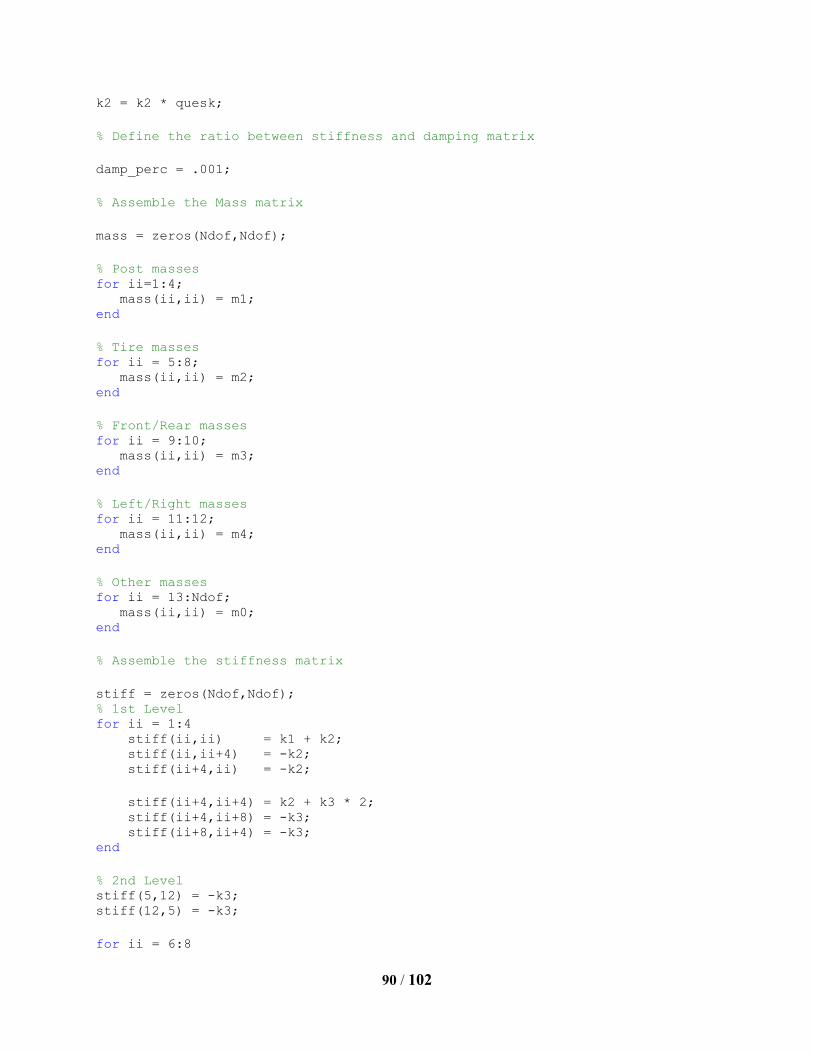
90 / 102
k2 = k2 * quesk;
% Define the ratio between stiffness and damping matrix
damp_perc = .001;
% Assemble the Mass matrix
mass = zeros(Ndof,Ndof);
% Post masses for ii=1:4; mass(ii,ii) = m1; end
% Tire masses for ii = 5:8; mass(ii,ii) = m2; end
% Front/Rear masses for ii = 9:10; mass(ii,ii) = m3; end
% Left/Right masses for ii = 11:12; mass(ii,ii) = m4; end
% Other masses for ii = 13:Ndof; mass(ii,ii) = m0; end
% Assemble the stiffness matrix
stiff = zeros(Ndof,Ndof); % 1st Level for ii = 1:4 stiff(ii,ii) = k1 + k2; stiff(ii,ii+4) = -k2; stiff(ii+4,ii) = -k2;
stiff(ii+4,ii+4) = k2 + k3 * 2; stiff(ii+4,ii+8) = -k3; stiff(ii+8,ii+4) = -k3; end
% 2nd Level stiff(5,12) = -k3; stiff(12,5) = -k3;
for ii = 6:8

91 / 102
stiff(ii,ii+3) = -k3; stiff(ii+3,ii) = -k3; end
% 3rd kount = 3; for ii = 9:12 kount = kount + 1; stiff(ii,ii) = k3 * 2 + k0 * 2; stiff(ii,ii-4) = -k3; stiff(ii-4,ii) = -k3; if ii ~= 12 stiff(ii,ii-3) = -k3; stiff(ii-3,ii) = -k3; else stiff(ii,5) = -k3; stiff(5,ii) = -k3; end stiff(ii,(ii + kount):(ii + kount + 1)) = -k0; stiff((ii + kount):(ii + kount + 1),ii) = -k0; end
% 4th Level for ii = 13:20; stiff(ii,ii) = k0; end stiff(13:14,9) = -k0; stiff(9,13:14) = -k0; stiff(15:16,10) = -k0; stiff(10,15:16) = -k0; stiff(17:18,11) = -k0; stiff(11,17:18) = -k0; stiff(19:20,12) = -k0; stiff(12,19:20) = -k0;
% Assemble the damping matrix
damp = damp_perc * stiff;
% Assemble the matrix of zeros to build state space equations
null = zeros(Ndof,Ndof);
% Form 2N x 2N state space equation.
a = [null,mass;mass,damp]; b = [-mass,null;null,stiff]; [x,d] = eig(b,-a);
% Sort Modal Frequencies

92 / 102
orig_lambda = diag(d); [Y,I] = sort(imag(orig_lambda)); lambda = orig_lambda(I); xx = x(:,I);
% Normalize x matrix to real vectors if possible
NumPoles = length(lambda); if((NumPoles < 2 * Ndof) | (NumPoles > 2 * Ndof)), disp('Error - Number of poles found invalid') break end
for ii=1:2 * Ndof; xx(1:2 * Ndof,ii) = xx(1:2 * Ndof,ii) ./ xx(2 * Ndof,ii); end
% Compute 'modal a' and 'modal b' matrix
Ma = diag(xx.'* a * xx); Mb = (xx.'* b * xx);
% Extract modal vectors from state-space formulation
Psi(1:2 * Ndof / 2,:) = xx(2 * Ndof / 2 + 1:2 * Ndof,:);
clear a,clear b,clear x,clear d;
% Set up data type variables
NFmin = min(abs(imag(lambda ./ (2 * pi)))); NFmax = max(abs(imag(lambda) ./ (2 * pi))); disp([' Range of damped natural frequencies: ',... num2str(NFmin),' to ',num2str(NFmax),' (Hz)']) Fmin = input('Enter minimum frequency (Hz): (0)'); if isempty(Fmin),Fmin = 0;end; Fmax = input('Enter maximum frequency (Hz): (100)'); if isempty(Fmax),Fmax = 100;end; BS = input('Enter number of frequencies: (512)'); if isempty(BS),BS=512;end; Type_xva = input('Enter type of TF data (X/R=0, V/R=1, A/R=2): (2)'); if isempty(Type_xva) Type_xva = 2; end
frequency = linspace(Fmin,Fmax,BS); Omin = Fmin*(2*pi); Omax = Fmax*(2*pi); Omega = linspace(Omin,Omax,BS);
% Add random noise to FRF data?
RandomPercent=input('Enter random noise factor: (0.001)'); if isempty(RandomPercent),RandomPercent=0.001;end;

93 / 102
for ii=1:BS; FRF(:,:,ii) = inv(-mass.*omega(ii).*omega(ii) + damp.*j.*omega(ii) +
stiff)* ... (j*omega(ii))^Type_xva; %FRF in units requested end;
for ii=1:Ni for jj=No frf = squeeze(FRF(ii,jj,:)); irf = HP_ifft(frf,2); max_irf = max(abs(irf)) irf = irf+RandomPercent*max_irf*rand(size(irf));
frf = fft(irf); FRF(ii,jj,:) = frf(1:BS); %ii,jj end end
% Set up PsiDOF array (default to x direction)
for ii=1:Ndof PsiDOF(ii,1) = ii; PsiDOF(ii,2) = 1; end
% Plot requested FRF measurement to screen
scale = 360.0 / (2.0*pi); chk = 0; while(chk == 1) kk = input('Plot FRFs (Yes=1): (0)'); if isempty(kk),chk = 0; end; if isempty(kk),break; end;
ii=input('Input DOF: (1)');
if isempty(ii),ii = 1; end;
jj=input('Output DOF: (1)');
if isempty(jj),jj = 1; end;
H = squeeze(FRF(jj,ii,:)); figure; subplot(211),semilogy(frequency,abs(H)) xlabel('Frequency (Hz)'),ylabel('Magnitude'),grid title(['FRF: H(',num2str(jj),',',... num2str(ii),')']) subplot(212),plot(frequency,scale.*angle(H)) xlabel('Frequency (Hz)'),ylabel('Phase'),grid end

94 / 102
freqax = linspace(Fmin,Fmax,BS - 1); radax = freqax * 2 * pi; for ii = 1:4 for jj = 1:Ndof TRF(jj,ii,:) = squeeze(FRF(jj,ii,2:end)) ./
squeeze(FRF(ii,ii,2:end)); % Give A/A (ft/s^2 / ft/s^2) TRF(jj,ii,:) = squeeze(TRF(jj,ii,:)) .* radax' .* radax' .* -1; %
Mult by j*omega squared which gives A/X (ft/s^2 / ft) end end
TRF = TRF ./ 32.2; % 'A' Units from ft/s^2 to G's
TRF = TRF ./ 12; % 'X' Units from ft to in
% Mass Legend % =========== % m1-m4 Shaker Post Mass % m5-m8 Un-Sprung Mass at Each Corner % m9-m10 Mass of Front/Rear % m11-m12 Mass of Left/Right % m13-m20 Various Other Masses
figure(1) subplot(211) semilogy(freqax,abs(squeeze(TRF(1,1,:)))) hold all; xlabel('Frequency (Hz)') ylabel('Magnitude (G''s/inch)') title(sprintf('Driving Point Transmissibility\nAt The Wheel Pan')) grid on box on ylim([10^-4 10^2])
subplot(212) plot(freqax,unwrap(angle(squeeze(TRF(1,1,:)))).*180./pi) hold all; xlabel('Frequency (Hz)') ylabel('Phase (degrees)') ylim([-200 200]) set(gca,'YTick',-180:90:180) grid on box on
figure(2) subplot(211) semilogy(freqax,abs(squeeze(TRF(5,1,:)))) hold all; xlabel('Frequency (Hz)') ylabel('Magnitude (G''s/inch)') title(sprintf('Wheel/Wheelpan Transmissibility')) grid on box on ylim([10^-2 10^3])

95 / 102
subplot(212) plot(freqax,angle(squeeze(TRF(5,1,:))).*180./pi) hold all; xlabel('Frequency (Hz)') ylabel('Phase (degrees)') ylim([-200 200]) set(gca,'YTick',-180:90:180) grid on box on
figure(3) subplot(211)
semilogy(freqax,abs(squeeze(TRF(9,1,:)))) hold all; xlabel('Frequency (Hz)') ylabel('Magnitude (G''s/inch)') title(sprintf('Fwd. Vehicle Structure/Wheelpan Transmissibility')) grid on box on ylim([10^-4 10^2])
subplot(212) plot(freqax,angle(squeeze(TRF(9,1,:))).*180./pi) hold all; xlabel('Frequency (Hz)') ylabel('Phase (degrees)') ylim([-200 200]) set(gca,'YTick',-180:90:180) grid on box on
figure(4) subplot(211) semilogy(freqax,abs(squeeze(TRF(11,1,:)))) hold all; xlabel('Frequency (Hz)') ylabel('Magnitude (G''s/inch)') title(sprintf('Left Vehicle Structure/Wheelpan Transmissibility')) grid on box on ylim([10^-4 10^2])
subplot(212) plot(freqax,angle(squeeze(TRF(11,1,:))).*180./pi) hold all; xlabel('Frequency (Hz)') ylabel('Phase (degrees)') ylim([-200 200]) set(gca,'YTick',-180:90:180) grid on
box on

96 / 102
Appendix G. Principal Reference and Response MATLAB® Code
% % Transmissibility Project Script - March 2013 % %************************************************************************** % Authors: Allyn Phillips * % Randall Allemang - [email protected] * % Thomas Steed - [email protected] * % Matthew Allemang - [email protected] * % Date: 17-Aug-06 % Modified: 03-Mar-13 % Structural Dynamics Research Lab * % University of Cincinnati * % Cincinnat, Ohio 45221-0072 * % TEL: 513-556-2725 * % FAX: 513-556-3390 * %**************************************************************************
%%%%%%%%%%%%%%%%%%%%%%%%%%%%%%%%%%%%%%%%%%%%%%%%%%%%%%%%%%%%%%%%%%%%%%%%%%% % Bring in *.SDF File % Open file and identify number of channels and number time points clear all; close all; [filename, pathname] = uigetfile({'*.sdf','SDF Files (*.sdf)'},'Select SDF
Data File'); if(filename == 0), return, end;
clear options % options.chans = 0:2; options.offset = 0; options.length = 1024; options.chans = []; % null ... all channels
sdf = readDXopen([pathname filename],options); sdf = readDXdata(sdf,options); sdf = readDXclose(sdf,options);
nTimePts = double(sdf.dataHdr.num_of_points * sdf.scanBig.num_of_scan); nChans = length(sdf.chanNum);
Tmin = 0; SampleRate= 1 / (sdf.xdata(2) - sdf.xdata(1)); Tmax = nTimePts / SampleRate; Fmin = 0; Fmax = 0.8 * SampleRate / 2;
disp(['SDF File Information: ' ]); disp([' ' ]);
disp(['Number of time points: ' num2str(nTimePts)]); disp(['Number of channels: ' num2str(nChans)]);

97 / 102
disp(['Sample rate: ' num2str(SampleRate) ' Samples/Second']);
disp(['Starting Time: ' num2str(Tmin)]); disp(['Ending Time: ' num2str(Tmax) ' Seconds']); disp(['Minimum Frequency: ' num2str(Fmin) ' Hz']); disp(['Maximum Frequency: ' num2str(Fmax) ' Hz']); disp([' ' ]);
%%%%%%%%%%%%%%%%%%%%%%%%%%%%%%%%%%%%%%%%%%%%%%%%%%%%%%%%%%%%%%%%%%%%%%%%%%%%%
%%%%%%%%%%%% % Load Channel Info FileLoad = input('Load Excel Calibration/Info File (0=No, 1=Yes) (1) '); if isempty(FileLoad),FileLoad = 1, end; if(FileLoad==1),
%%%%%%%%%%%%%%%%%%%%%%%%%%%%%%%%%%%%%%%%%%%%%%%%%%%%%%%%%%%%%%%%%%%%%%%%%%%%%
%%%%%%%%%%%% % Squeak & Rattle Sensor and Geometry Array Creation from Excel % ------------------------------------------------------------- [filename1,pathname1] = uigetfile('*.xls','Excel File (X-Modal UFF
default format):'); if (filename1 == 0),return; end; [aa,bb,cc] = xlsread([pathname1 filename1],'Sensor Information');
%%%%%%%%%%%%%%%%%%%%%%%%%%%%%%%%%%%%%%%%%%%%%%%%%%%%%%%%%%%%%%%%%%%%%%%%%%%%%
%%%%%%%%%%%%
%%%%%%%%%%%%%%%%%%%%%%%%%%%%%%%%%%%%%%%%%%%%%%%%%%%%%%%%%%%%%%%%%%%%%%%%%%%%%
%%%%%%%%%%%% % While Loop To Break if Excel Channels Do Not Match Channels in SDF % ------------------------------------------------------------------
% condition=1; % while(condition==1); % excel_channels=length(aa); % if excel_channels==nChans % condition=0; % else % disp('Excel File Problem: Channel Mismatch!') % break % end % end else % Set defaults if no Excel file loaded aa = zeros(nChans,7); bb = cell(nChans+2,7);
aa(:,1) = [1:nChans]; % Channel Number Defaults aa(:,2) = [1:nChans]; % Point (DOF) Number Defaults aa(:,3) = 1; % Point (DOF) Direction Defaults aa(:,4) = 12; % Data Type Code [bb{:,5}] = deal('-1'); % Model Number aa(:,6) = -1; % Serial Number aa(:,7) = 1.0; % Calibration (Volts/EU)

98 / 102
end
%******************************** % Now check for valid entrys %***********************************
Chans = aa(:,1); % Channel Number Defaults DOFs = aa(:,2); % Point (DOF) Number Defaults DOFdirs = aa(:,3); % Point (DOF) Direction Defaults DataType = aa(:,4); % Data Type Code ModelNum = bb(:,5); % Model Number SerialNum = aa(:,6); % Serial Number Cal = aa(:,7); % Calibration (Volts/EU)
for ii=1:nChans if(isnan(Chans(ii))),disp('Excel File Problem: Channel
NaN'),Chans(ii)=0;,end; if(isnan(DOFs(ii))),disp('Excel File Problem: DOF NaN'),DOFs(ii)=0;,end; if(isnan(DOFdirs(ii))),disp('Excel File Problem: DIR
NaN'),DOFdirs(ii)=0;,end; if(isnan(DataType(ii))),disp('Excel File Problem: Data Type
NaN'),DataType(ii)=0;,end; if(isempty(ModelNum(ii))),disp('Excel File Problem: Model Number
NaN'),ModelNum(ii)='NONE';,end; if(isnan(SerialNum(ii))),disp('Excel File Problem: Serial Number
NaN'),SerialNum(ii)=-1;,end; if(isnan(Cal(ii))),disp('Excel File Problem: Calibration
NaN'),Cal(ii)=1.0;,end; end;
%%%%%%%%%%%%%%%%%%%%%%%%%%%%%%%%%%%%%%%%%%%%%%%%%%%%%%%%%%%%%%%%%%%%%%%%%%%%%
%%%%%%%%%%%%
%%%%%%%%%%%%%%%%%%%%%%%%%%%%%%%%%%%%%%%%%%%%%%%%%%%%%%%%%%%%%%%%%%%%%%%%%%%%%
%%%%%%%%%%%% % Default Settings For Setup Menu % ------------------------------- BS = 2048; nshftperc = 50; Ns = round(0.8 * (BS / 2)); nShft = BS * (nshftperc / 100);
ID_one = 'NONE'; ID_two = 'NONE';
% Default to first 4 channels as references
Nr = 4; No = nChans; No = 154; % Some error in the last few channels. Lets Just use 154 Win_code = 110;
% outputs = Chans; outputs = [1:No]'; references = [1:4];

99 / 102
save Sponsor_defaults BS nshftperc Ns nShft ID_one ID_two No outputs Nr
references Win_code %%%%%%%%%%%%%%%%%%%%%%%%%%%%%%%%%%%%%%%%%%%%%%%%%%%%%%%%%%%%%%%%%%%%%%%%%%%%%
%%%%%%%%%%%% %%%%%%%%%%%%%%%%%%%%%%%%%%%%%%%%%%%%%%%%%%%%%%%%%%%%%%%%%%%%%%%%%%%%%%%%%%%%%
%%%%%%%%%%%% % Setup Menu % ---------- setup = 1; while(setup == 1), op_code = menu('Enter Setup Option: ', ... 'Load Default Settings',... 'Load Previous Settings',... ['Time Domain Blocksize: ',sprintf('%5.0f',BS)], ... ['# of References : ',sprintf('%5.0f',Nr)], ... ['# of Outputs: ',sprintf('%5.0f',No)], ... ['Percent Overlap: ',sprintf('%5.0f',nshftperc)],... ['Window Type: ',sprintf('%5.0f',Win_code)], ... ['Test Vehicle Model: ', ID_one], ... ['Test Description: ', ID_two], ... 'Measure / Execute ! ', ... 'EXIT');
drawnow;
if(op_code == 1), load Sponsor_defaults end
if(op_code == 2), load Sponsor_previous end
if(op_code == 3), BS = input('Enter Time Blocksize: (2048) '); if isempty(BS),BS = 2048, end; end
if(op_code==4), Nr = input('Enter Number of References: (16) '); if isempty(Nr),Nr = 16,end;
references=input('Enter Input Channel Number(s): ([1:4]) '); if isempty(references),inputs = [1:4],end; end
if(op_code == 5), No=input('Enter Number of Outputs: (16) '); if isempty(No),No = 16,end;
outputs = input('Enter Output Channel Number(s): ([1:16]) '); if isempty(outputs),outputs = [1:16],end; end

100 / 102
if(op_code == 6), nshftperc=input('Enter Percent Overlap: (50) '); if isempty(nshftperc),nshftperc = 50, end; end
if(op_code == 7), Win_code = input('Enter DSP Window Type:(001 or 110) '); if isempty(Win_code),Win_code=001,end; end
if(op_code == 8), ID_one = input('Enter Vehicle Model in Single Quotes: (Vehicle Z) '); if isempty(ID_one),ID_one = 'Vehicle Z',end; end
if(op_code == 9), ID_two = input('Enter Test Description in Single Quotes: '); if isempty(ID_two),ID_two = 'Test Data Run',end; end
if(op_code == 10), setup = 0; end if(op_code == 11), return end end drawnow save Sponsor_previous BS nshftperc Ns nShft ID_one ID_two No outputs Nr
references Win_code %%%%%%%%%%%%%%%%%%%%%%%%%%%%%%%%%%%%%%%%%%%%%%%%%%%%%%%%%%%%%%%%%%%%%%%%%%%%%
%%%%%%%%%%%% %%%%%%%%%%%%%%%%%%%%%%%%%%%%%%%%%%%%%%%%%%%%%%%%%%%%%%%%%%%%%%%%%%%%%%%%%%%%%
%%%%%%%%%%%% % Windows % ------- wnd = ones(1,BS); if(Win_code==110) wnd = (cos(2*pi*(0:(BS-1))/BS) - wnd)/2; % Hanning else wnd = ones(1,BS); % Rectangular end %%%%%%%%%%%%%%%%%%%%%%%%%%%%%%%%%%%%%%%%%%%%%%%%%%%%%%%%%%%%%%%%%%%%%%%%%%%%%
%%%%%%%%%%%%
nEns = fix((nTimePts-BS) / nShft);
if nEns > 300 nEns = 300; % Limit Averages For Large Data sets. (Don't have ALL day) end
Grr = zeros(No,Nr,Ns);

101 / 102
% Do Principal References and PRFs
options.offset = 0; options.length = BS; options.chans = []; % null ... all channels
sdf = readDXopen([pathname filename],options);
Grr(No,Nr,Ns)=0+j*eps;
for ii = 1:nEns, ii options.offset = (ii-1)*nShft; sdf = readDXdata(sdf,options);
% Multiply by window % Calibrate for sensor sensitivity (Cal in Volts/EU) % Calibrate for FFT blocksize for jj = 1:nChans, Sx(jj,:) = fft(sdf.ydata(jj,:) .* (wnd/(Cal(jj)*BS/2))); end
% Sx = 1/(BS/2)*fft(sdf.ydata,[],2);
for jj = 1:Ns, Grr(1:No,1:Nr,jj) = Grr(1:No,1:Nr,jj) + Sx(outputs,jj) *
Sx(references,jj)'; end
end sdf = readDXclose(sdf,options);
f = (0:(Ns-1)) / (sdf.xdata(end)+sdf.xdata(2)-2*sdf.xdata(1)); Grr = Grr / nEns;
drawnow
figure semilogy(f,abs(squeeze(Grr(1,1,:)))); semilogy(f,abs(squeeze(Grr(2,2,:)))); semilogy(f,abs(squeeze(Grr(3,3,:)))); semilogy(f,abs(squeeze(Grr(4,4,:)))); title(sprintf('Grr\n%s',strrep(filename,'_','\_'))); xlabel('Frequency (Hz)') ylabel('Magnitude (in^2)') xlim([0 100]);
for ii = 1:Ns [u,s,v] = svd(squeeze(Grr(1:4,1:4,ii))); Vref(1:4,ii) = diag(s); end
figure semilogy(f,Vref(1,:));

102 / 102
hold all; semilogy(f,Vref(2,:)); semilogy(f,Vref(3,:)); semilogy(f,Vref(4,:)); title(sprintf('Principal References\n%s',strrep(filename,'_','\_'))); xlabel('Frequency (Hz)') ylabel('Magnitude (in^2)') xlim([0 100]); grid on; box on;
% Principal Response Functions Goo = squeeze(Grr(5:154,1,:)); Goo = cat(1,Goo,squeeze(Grr(5:154,2,:))); Goo = cat(1,Goo,squeeze(Grr(5:154,3,:))); Goo = cat(1,Goo,squeeze(Grr(5:154,4,:)));
[u,s,v] = svd(Goo','econ'); s2 = s; s2(300:end,300:end) = 0; PRF = u * s2;
figure semilogy(f,abs(PRF(:,1:25))); title(sprintf('Principal Response Functions
[25]\n%s',strrep(filename,'_','\_'))); xlabel('Frequency (Hz)') ylabel('Magnitude (in^2)') xlim([0 100]); box on;
figure semilogy(f,abs(PRF(:,1:300))); title(sprintf('Principal Response Functions
[300]\n%s',strrep(filename,'_','\_'))); xlabel('Frequency (Hz)') ylabel('Magnitude (in^2)') xlim([0 100]); box on;