comparison of bubble and sheet cavitation...
TRANSCRIPT
1
Cav03-OS-1-008 Fifth International Symposium on Cavitation (cav2003)
Osaka, Japan, November 1-4, 2003
COMPARISON OF BUBBLE AND SHEET CAVITATION MODELS FOR SIMULATION OF CAVITATING FLOW OVER A HYDROFOIL
Takafumi Kawamura University of Tokyo
Motoyuki Sakoda University of Tokyo
ABSTRACT In this work, we have applied a new hybrid type sheet
cavitation model to the CAV2003 workshop test case. The new model is essentially a combination of an interface tracking sheet cavity model and a bubbly flow mixture model. The results are compared with a bubble dynamics based cavitation model implemented in a commercial code Fluent 6.1.
The predicted sizes of the cavity by the two models were found to be very different. In two cavitation cases, σR=0.4 and σR=0.8, the new sheet cavity model predicted larger mean cavity size. Accordingly predicted mean CL and CD values were also larger. In the case σR=0.4, both model predicted almost steady cavity shape, while in the case σR=0.8 the results of the sheet cavity model exhibited strongly unsteady behavior.
INTRODUCTION
Numerical modeling of cavitating flow is difficult in many aspects. First, cavitating flow involves wide range of spatial and temporal scales. Usually there is several orders of magnitude difference between the global scale such as the scale of the hydrofoil chord and that of cavitation bubbles. Another important nature is that it can take different flow regimes such as bubble or sheet cavitation. Those two types of cavitation are very different in spatial and temporal scales, and this makes it difficult to apply a single model.
Existing cavitation models can be roughly categorized into two groups. One is interface tracking approach in which sheet cavity is treated as pure vapor. This kind of approach has been mainly used in combination with potential flow based boundary element methods [1, 2], but has not been practically used with viscous flow simulation methods. Another approach which is more often used in CFD methods is the multiphase flow approach in which cavitating flow is usually modeled as variable density mixture fluid[3-7], and variation of the mixture density is modeled by constitutive equations based either on bubble dynamics[3, 4, 6] or on equilibrium assumptions[5, 7].
Those cavitation models based on bubble dynamics have been applied to unsteady cavitation over a NACA0015 hydrofoil, but the length of the cavity was underestimated and unsteady nature of cavitation was not well reproduced [3, 4, 8]. The investigated case involves both sheet and bubbly cloud cavity,
and the results of the preceding works suggest a possibility that the use of bubbly flow model based on the Rayleigh-Plesset equation is not appropriate in the sheet cavity regime.
Based on the above assumption, a new model has been developed in this study. The new model is a combination of the interface tracking approach and the bubbly flow model. The sheet cavity part of which spatial and temporal scales are close to those of the hydrofoil is explicitly modeled by an interface tracking method, while the bubbly flow part in which evaporation and condensation take place in scales smaller than computational mesh is modeled by a bubble flow model. It is expected that this model complements the interface tracking methods in dealing with the problems associated with the cavity inception and closure.
In this paper, the new model is applied to the CAV2003 workshop test case. The results are compared with those obtained by a commercial code Fluent 6.1 implementing the full cavitation model proposed by Singhal et al. [6] which is one of the models based on bubble dynamics.
NOMENCLATURE
CL lift coefficient mµ viscosity of mixture
CD drag coefficient tµ eddy viscosity
Cp pressure coefficient vr
velocity vector
Rσ cavitation number mρ density of mixture
N Bubble number density lρ density of water
R bubble radius gρ density of vapor
α vapor volume fraction V integral total volume of vapor
St Strouhal number
NUMERICAL METHOD
Fluent mixture modelFluent mixture modelFluent mixture modelFluent mixture model Two different cavitation models are applied to the CAV2003
test case in this study. One is the cavitation model of a commercial CFD code Fluent version 6.1 based on the “full
2
cavitation model” proposed by Singhal et al. [6]. Fluent is an unstructured mesh based finite volume code, and detailed descriptions of the numerical method are found in publications such as Kim [9]. The k-ω turbulence model [10] was chosen as the turbulence model. A segregated solver with SIMPLE as the velocity-pressure coupling algorithm was selected, and QUICK scheme was used for the discretization of the momentum equation in this study.
The model has been successfully applied to cavitating flows over a hydrofoil and marine propellers [11]. The extension of the cavitation model made by Fluent is the introduction of the velocity slip between liquid and gas phases. However, the influence of the slip velocity was found to be negligible for the cases investigated in this study. Therefore we can assume that this model is essentially the same as the original full cavitation model of Singhal et al [6].
Sheet cavity modelSheet cavity modelSheet cavity modelSheet cavity model
The second model used in this study is an original model based on the combination of a mixture type model and a free-surface model. The base flow solver is a structured grid based finite volume code developed by Kawamura [12, 13]. Since detailed description and validation of the code are found in the preceding publications [12, 13], only the extension to cavitating flows is described in this paper. In this model, cavitating flow is modeled as bubbly mixture and pure vapor zone clearly separated by the moving interfaces as shown in Fig. 1.
vapor P =PvvaporP =Pv
mixture
interface
flow
FigureFigureFigureFigure 1 Description of the sheet cavity model 1 Description of the sheet cavity model 1 Description of the sheet cavity model 1 Description of the sheet cavity model
The governing equations for the bubbly mixture zone are the conservation equations for the mass and momentum of the mixture such as
( ) ( ) 0=⋅∇+∂∂
vt mm
rρρ (1)
and
( ) ( )
( ) ( )
⋅∇−∇+∇+⋅∇+−∇=
⋅∇+∂∂
Ivvvp
vvvt
TTm
mm
rrr
rrr
3
2µµ
ρρ (2)
The mass transfer is modeled by a simple model based on the Rayleigh-Plesset equation:
( )
>−
−
≤−
=⋅∇+∂∂
)(3
)(2
)(3
)(2
vv
vv
pppp
pppp
vRt
R r (3)
The vapor volume fraction and the density of the mixture are calculated using the following relations:
3
4 3NRπα = (4)
αραρρ glm +−= )1( (5)
The bubble number density is assumed to be uniform. At the cavity interface, the following simplified free-surface boundary conditions are imposed.
vpp = (6)
0=∂∂n
vv
(7)
in which n denotes the direction normal to the interface pointing towards the vapor zone. The interface location is tracked by the level-set method [14], in which the interface is represented as the iso-surface of the level-set function φ = 0, and the temporal evolution of φ is governed by the following convection equation:
( ) 0=⋅∇+∂∂
vt
rφφ (8)
Once the cavity interface is formed, the interface moves with the local velocity of the mixture, but Eq. (8) can not generate a new interface. Therefore, the initial cavity is provided in the computational cell where the void ratio α given by the mixture mass transfer model Eq. (3-5) exceeds a given threshold value αs.
The k-ω turbulence model is used for turbulence closure. A second order central scheme is used for the discretization in space except for the convective terms. The convective term in the momentum equation is discretized by the QUICK scheme, while a first order upwind scheme is used for the convective terms in Eq. (3) and the turbulence model. A fractional step type segregated algorithm is used for the time integration. A first order implicit scheme is used for non-cavitating flow and a second order semi-implicit scheme is used for cavitation problems.
RESULTS
NonNonNonNon----cavitating flow (condition #0)cavitating flow (condition #0)cavitating flow (condition #0)cavitating flow (condition #0)
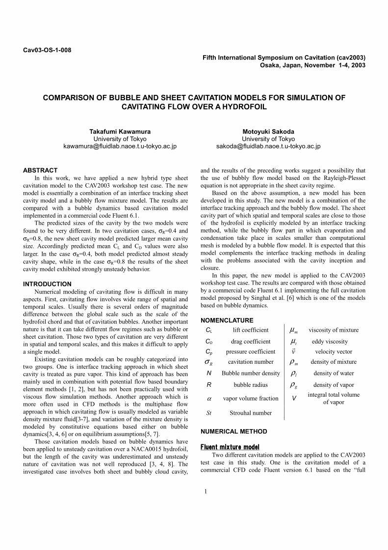
A detailed grid study was carried out for the non-cavitating flow past the CAV2003 hydrofoil using the research code in which the sheet cavity model is implemented. The flow geometry, the inlet and outlet conditions comply with the workshop specification. The so-called C-grid topology was adopted, and the boundary condition used in the simulations is shown in Figure 2. The total of 16 grids were used to investigate the influence of grid parameters such as the number of control volumes in the circumferential direction Ni and that in the radial direction Nj, the minimum grid spacing in the radial direction at the leading edge ∆ηLE and a the trailing edge ∆ηTE, and the minimum spacing in the circumferential direction at the leading edge ∆ξLE and at the trailing edge ∆ξTE. The grids were generated by an algebraic method. A typical grid (GRID 3) is shown in Figure 3.
The values of the parameters and the computed drag and lift coefficients are summarized in Table 1. All the variables are non-dimensionalized with respect to the chord length, the free stream velocity and the density of water unless otherwise mentioned. The relation between the grid parameters and the computed lift

3
and drag coefficients is shown in Figures 4 to 7. The computed lift and drag coefficients were found to be not very sensitive to the minimum grid spacing at the trailing edge probably due to the larger boundary layer thickness, while the spacing near the leading edge is very important. The grid study showed that rather small grid number 256× 64 is sufficient if appropriate minimum spacing is used. The required minimum spacing at the leading edge is determined to be 4101 −× in the radial direction and
3101 −× in the chord direction. The corresponding +y , the
distance from the wall to the first grid points in viscous unit, is on the order of unity. Based on this result, GRID 3 was chosen for the simulations of following cavitation cases.
The non-cavitating case was also computed by Fluent 6.1 using the grid parameters for GRID 3, and by a boundary element code [15] based on the potential flow and boundary layer theory. Table 2 shows comparisons of the computed lift and drag coefficients along with the CPU time required for the lift coefficient to reach 99.9% of the converged value on a workstation with an Intel Xeon 2.8GHz CPU. The comparison of the pressure coefficient on the foil surface in Figure 8 shows that the Cp distribution is globally in good agreement but small difference exists near the leading and trailing edges. The Cp distribution computed by the BEM code is a little different at the trailing edge from that from the two CFD codes probably because of the use of Kutta condition. On the other hand, the peak of the negative pressure near the leading edge is smaller in Fluent. This is probably due to differences in the implementation of the k-ω turbulence model, and more detailed examinations are being carried out at present. Those differences resulted in the difference in the lift and drag coefficients.
Table 1 Parameters for the grid studyTable 1 Parameters for the grid studyTable 1 Parameters for the grid studyTable 1 Parameters for the grid study GRID ni nj ∆η at LE ∆η at TE ∆ξ at LE ∆ξ at TE CD CL
1
2
3
4
5
6
7
8
9
10
11
12
13
14
15
16
512
256
256
256
256
256
256
256
256
128
512
256
256
256
256
256
256
64
64
64
64
64
32
16
128
64
64
64
64
64
64
64
5100.1 −× 4100.1 −× 4100.1 −× 4100.1 −× 4100.1 −× 4100.1 −× 4100.2 −× 4100.5 −× 5100.5 −× 4100.1 −× 4100.1 −× 4100.1 −× 4100.1 −× 4100.1 −× 4100.1 −× 4100.7 −×
5100.5 −× 5100.3 −× 4103.2 −× 3105.1 −× 4100.9 −× 4103.2 −× 4109.4 −× 3100.1 −× 4100.1 −× 4103.2 −× 4103.2 −× 4103.2 −× 4103.2 −× 4103.2 −× 4103.2 −× 4103.2 −×
3100.1 −× 3100.1 −× 3100.1 −× 3100.1 −× 3100.1 −× 3100.1 −× 3100.1 −× 3100.1 −× 3100.1 −× 3108.1 −× 4105.4 −× 3105.4 −× 4105.4 −× 3101.1 −× 4105.9 −× 4105.9 −×
3100.1 −× 2100.1 −× 2100.1 −× 2100.1 −× 2100.1 −× 2100.1 −× 2100.1 −× 2100.1 −× 2100.1 −× 2108.1 −× 3105.4 −× 3100.9 −× 2100.1 −× 3101.1 −× 2100.2 −× 2100.2 −×
0.0148
0.0144
0.0140
0.0299
0.0173
0.0140
0.0149
0.0385
0.0143
0.0120
0.0147
0.0117
0.0142
0.0136
0.0142
0.0205
0.6687
0.6763
0.6733
0.6456
0.6619
0.6717
0.6738
0.5605
0.6696
0.6831
0.6780
0.6402
0.6741
0.6827
0.6813
0.5940
Table 2 Comparison of CTable 2 Comparison of CTable 2 Comparison of CTable 2 Comparison of CLLLL and C and C and C and CDDDD for non for non for non for non----cavitating casecavitating casecavitating casecavitating case
Fluent SCM BEM
CL 0.64 0.67 0.75
CD 0.0183 0.0140 0.0136CPU time 473 s 240 s 0.14 s
Figure 2 Boundary conditions
Cavitating flow (condition #1 and #2)Cavitating flow (condition #1 and #2)Cavitating flow (condition #1 and #2)Cavitating flow (condition #1 and #2)
Two cavitating conditions, σR=0.8 and 0.4, computed by Fluent 6.1 mixture model and the sheet cavity model. Fluent implements both steady and unsteady formulations, but even with the unsteady formulation the computed flow was quite stable and no significant difference from the steady flow calculation was observed. Therefore, only the results from the steady flow simulations are shown for Fluent mixture model, while the sheet cavity model is implemented only in unsteady formulation, and both time-dependent and time-averaged results are shown.
In Fluent 6.1 mixture model, users can choose whether the slip velocity between the liquid and gas phases is considered or not. However, for the present case, it was confirmed that the result is not sensitive to this choice. Another important parameter in Fluent 6.1 mixture model is the mass fraction of the non condensable gas (NCG). We found that the result is quite sensitive to the value of NCG. Based on preliminary test computations, the value 1× 10⁻⁶, which is also the recommended value in the original paper [6], was found to give reasonable results and used for the computations presented in this paper. In the sheet cavity model, arbitrary parameters are the threshold void ratio αs for making a new cavity cell and the bubble number density N. Although, the values 0.8 and 1 × 10⁵ are used respectively, it was confirmed that the results are not sensitive to the choice of these parameters. The time step for the unsteady computation was set to 5× 10⁻⁵.
The converged non-cavitating flow was used as the initial condition for velocity, pressure and turbulence fields. The unsteady flow simulations by the sheet cavity model were continued to t=48 at σR=0.8 and to t=25 at σR =0.4, while the steady flow simulations by Fluent were stopped when the steady state was reached. The CPU time required for the unsteady computation to t=48 was about 80 hours, which is more than 1000 times longer than that for the steady non-cavitating flow computation, while that for steady cavitating flow simulation by Fluent was about an hour, which is about eight times the non-cavitation flow simulation.
The time histories of the integral total volume of vapor per unit meter span computed by the sheet cavity model are shown in Figure 9. The plot clearly indicates that there is quasi-periodical growth and disappearance of the vapor volume in the case σR=0.8, while at σR=0.4 the vapor volume is almost constant after reaching a steady state. The period for the vapor volume fluctuation at σR=0.8 was about 7.0.
The time histories of the lift and drag coefficients computed by the sheet cavity model at σR=0.8 and σR=0.4 are shown in

4
Figures 10 and 11, respectively. The fluctuation of the lift and drag forces is small at σR=0.4, while at σR=0.8, the forces vary strongly in the same manner as the vapor volume. The largest and the smallest lift and drag forces almost synchronize with the largest and the smallest vapor volume in time.
Figure 12 shows the instantaneous fields of Cp and vapor volume fraction computed by the sheet cavity model for four time levels, t=13, 15, 17, and 19 in the case σR=0.8. The first two figures (a) at t=13 and (b) at t=15 show the growing phase of the sheet cavity; the third one (c) at t=17 corresponds the maximum cavity size, and the last one (d) shows the collapsing phase. It is noted that the vapor volume fraction is either 1.0 or less than 0.1 in most region meaning that “sheet cavity” modeled by the level-set method accounts for most cavity volume. This sequence of the figures shows that the length of the sheet cavity grows gradually until the cavity trailing edge almost reaches the end of the foil, and then a reverse flow emerges near the foil trailing edge. The reverse flow propagates towards the leading edge along the back surface of the foil causing the collapse of the sheet cavity. The collapsing sheet cavity is partially shed as detached cavity as shown in Figure 12 (d). Figure 12 (c) suggests that the source of the reverse flow is the flow along the face side of the foil which normally detaches at the trailing edge. It is supposed that the change in the pressure distribution near the trailing edge due to the extension of the sheet cavity triggers this reverse flow.
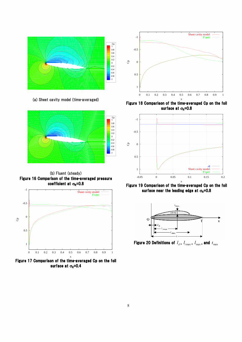
Hereafter, time-averaged quantities are shown. Figure 13 shows the comparison of the time-averaged vapor volume fraction computed by the sheet cavity model and Fluent mixture model for σR=0.4. The length of the cavity is very different between the two models. In the sheet cavity model, the back surface is completely covered with vapor, while in Fluent mixture model the length is shorter and the void ratio in the cavity is lower. Figure 14 shows the same comparison for σR=0.8. Similarly, the mean cavity length predicted by the sheet cavity model is larger. Comparisons of the time-averaged pressure coefficient are shown in Figures 15 and 16 for σR=0.4 and σR=0.8, respectively. Difference in the pressure coefficient corresponds to that in the void ratio. The time-averaged pressure coefficient on the foil surface is compared in Figures 17 for σR=0.4. The time-averaged pressure coefficient is equal to –σR on the entire back surface in the sheet cavity model simulation because the entire back surface is covered with vapor, while in Fluent simulation the pressure coefficient starts increasing after about 40% chord position. This corresponds to the shorter cavity length. Difference in Cp on the face side is found to be much smaller. The same comparison is shown in Figure 18 for σR=0.8. The tendency is similar to that for σR=0.4. Another difference between the two models is the pressure coefficient under the cavity. Figure 19 shows the time-averaged pressure coefficient near the leading edge for σR=0.8. It is noted that the pressure coefficient under the attached cavity is a little lower than -σR in Fluent, while in the sheet cavity model the overshoot in negative pressure is seen only in the vicinity of the leading edge. This is due to the different formulations in the cavitation models. Similar overshoot in the negative pressure on the back surface is also seen in the original paper by Singhal et al. [6].
The summary of the time-averaged quantities is shown in Table 3. The definitions of the parameters associated with the mean cavity shape are given in Figure 20. The over-line means that the variable is normalized by the chord length. These quantities indicate the cavity size predicted by the sheet cavity model is larger, and the lift and drag coefficients are also larger because of the larger cavity size. The Strouhal number calculated by the sheet cavity model in the case σR=0.8 was 0.14, which is lower than the value of around 0.2 reported in the past experimental studies [8, 16] for several foil sections and flow conditions.
Table 3 Comparison of the time Table 3 Comparison of the time Table 3 Comparison of the time Table 3 Comparison of the time----averaged quantitiesaveraged quantitiesaveraged quantitiesaveraged quantities
4.0=Rσ 8.0=Rσ
Fluent SCM Fluent SCM
CL 0.187 0.226 0.399 0.537
CD 0.063 0.233 0.047 0.086
dl 0.002 0.003 0.001 0.005
maxl 0.865 1.292 0.492 0.966
maxt 0.102 0.182 0.055 0.136
maxtl 0.507 0.988 0.393 0.794
V 1.77 10.00 0.65 3.17
S N.A. N.A. N.A. 0.14
SUMMARY In this work, we have applied the new hybrid type sheet
cavitation model to the CAV2003 workshop test case. The results are compared with the bubble dynamics based cavitation model implemented in Fluent 6.1. The predicted size of the cavity was very different. In two cavitating cases, σR=0.4 and σR=0.8, the sheet cavity model predicted larger mean cavity size. Accordingly predicted mean CL and CD values were also larger. In the case σR=0.4, both model predicted almost steady cavity shape, while in the case σR=0.8 the results of the sheet cavity model exhibited strongly unsteady nature.
Although it is difficult to make any conclusion without knowing experimental data, the results of the sheet cavitation model seem to be more reasonable. We have also applied the two models to NACA0015 case of which experimental data is available, and it was confirmed that the tendency was similar and that the prediction by the sheet cavity model was closer to experiments.
The main difference between the two models is in the treatment of the high void ratio region. In the bubbly flow model, the production rate of vapor decreases with increasing void ratio, but in the sheet cavity model growth of the sheet cavity is governed only by the dynamics of the liquid flow which is explicitly solved by the N-S equation. The results will be investigated further in detail when the experimental results become available.

5
ACKNOWLEDGMENTS This work was financed by the Grant-in-Aid for Scientific
Research (No. 14702055) of Ministry of Education, Culture, Sports, Science and Technology.
The authors would like to thank Prof. Hajime Yamaguchi for valuable discussions and providing the boundary element code. Fluent Inc. and Dr. Shin Hyung Rhee are also gratefully acknowledged for providing Fluent license and helpful suggestions.
REFERENCES 1. Kinnas, S. A., and Fine, N. E., Journal of Fluid Mechanics,
Vol. 254, 1993, pp.151-181. 2. Ando, J. and Nakatake, K., Proceedings of the Fourth
International Symposium on Cavitation, 2001, California Institute of Technology, Pasadena, CA USA.
3. Kubota, A. and Kato, H. and Yamaguchi, H., Journal of Fluid Mechanics, Vol. 240, 1992, pp.59-96.
4. Tamura, Y. and Sugiyama, K. and Matsumoto, Y., Proceedings of the Fourth International Symposium on Cavitation, 2001, California Institute of Technology, Pasadena, CA USA.
5. Reboud J-L. and Delannoy, Y., Proceedings of the Second International Symposium on Cavitation, Tokyo, Japan, 1994, pp 39-44.
6. Singhal, A.K., Athavale, M.M., Li, H.Y., and Jiang, Y., Journal of Fluids Engineering, Vol.124, 2001, pp. 617-624.
7. Iga, Y. and Nohmi, M. and Goto, A., and Shin, B. R. and Ikohagi, T., Proceedings of the Fourth International Symposium on Cavitation, 2001, California Institute of Technology, Pasadena, CA USA.
8. Yakushiji, R. and Yamaguchi, H. and Kawamura, T. and Maeda, M. and Sakoda, M., Journal of the Society of Naval Architects of Japan, Vol.190, 2001, pp.61-74 (in Japanese).
9. Kim, S.-E., Mathur, S.R., Murthy, J.Y., and Choudhury, D., AIAA Paper 98-0231, 36th AIAA Aerospace Sciences Meeting and Exhibit, Reno, NV, 1998.
10. Wilcox, D.C., Turbulence Modeling for CFD, Second Ed., DCW Industries, Inc., La Canada, CA, 1998.
11. Rhee, S., H., Kawamura, T., and Li, H., Proceedings of 8th International Conference on Numerical Ship Hydrodynamics, September 22-25, 2003, Busan, Korea.
12. Kawamura, T., Journal of Marine Science and Technology, Vol. 5 No. 3, 2000, pp. 112-122.
13. Kawamura, T., Journal of Marine Science and Technology, Vol. 5 No. 4, 2000, pp. 161-176.
14. Osher, S., Sethian, J.A., Journal of Computational Physics, Vol. 79, 1998, pp. 12-49.
15. Yamaguchi, H., http://www.fluidlab.naoe.t.u-tokyo.ac.jp/~yama/prog/prblg/index-e.html
16. Kawanami, Y., Kato, H. Yamaguchi, H., Tanimura, M., Tagaya, Y., Journal Fluids Engineering, Vol. 119 (4), 1997 , pp. 788-794.
X
Y
-6 -4 -2 0 2 4 6
-3
-2
-1
0
1
2
3
(a) Whole computational domain
X
Y
-0.5 0 0.5
-0.2
-0.1
0
0.1
0.2
(b) Near the hydrofoil
Figure 3 Grid system (GRID 3)Figure 3 Grid system (GRID 3)Figure 3 Grid system (GRID 3)Figure 3 Grid system (GRID 3)
0.5
0.55
0.6
0.65
0.7
0.75
0.8
0.85
0.9
0 100 200 300 400 5000
0.005
0.01
0.015
0.02
0.025
0.03
0.035
0.04
CL
CD
Number of points in ξ direction (Ni)
CLCD
Figure 4 Grid study: influence of Figure 4 Grid study: influence of Figure 4 Grid study: influence of Figure 4 Grid study: influence of NiNiNiNi (GRID 3, 10, 11) (GRID 3, 10, 11) (GRID 3, 10, 11) (GRID 3, 10, 11)
0.5
0.55
0.6
0.65
0.7
0.75
0.8
0.85
0.9
0 20 40 60 80 100 120 1400
0.005
0.01
0.015
0.02
0.025
0.03
0.035
0.04
CL
CD
Number of points in η direction (Nj)
CLCD
Figure 5 Grid study: influence of Figure 5 Grid study: influence of Figure 5 Grid study: influence of Figure 5 Grid study: influence of NjNjNjNj (GRID 3, 7, 8, 9) (GRID 3, 7, 8, 9) (GRID 3, 7, 8, 9) (GRID 3, 7, 8, 9)
6
0.5
0.55
0.6
0.65
0.7
0.75
0.8
0.85
0.9
1e-05 0.0001 0.0010
0.005
0.01
0.015
0.02
0.025
0.03
0.035
0.04
CL
CD
Minimum grid spacing in η direction at LE (∆ηLE)
CLCD
Figure 6 Grid study: influenFigure 6 Grid study: influenFigure 6 Grid study: influenFigure 6 Grid study: influence of ce of ce of ce of ∆η∆η∆η∆ηLELELELE(GRID 3, 7, 9, 16)(GRID 3, 7, 9, 16)(GRID 3, 7, 9, 16)(GRID 3, 7, 9, 16)
0.5
0.55
0.6
0.65
0.7
0.75
0.8
0.85
0.9
0.0001 0.001 0.010
0.005
0.01
0.015
0.02
0.025
0.03
0.035
0.04
CL
CD
Minimum grid spacing in ξ direction at LE (∆ξLE)
CLCD
Figure 7 Grid study: influence of Figure 7 Grid study: influence of Figure 7 Grid study: influence of Figure 7 Grid study: influence of ∆ξ∆ξ∆ξ∆ξLELELELE(GRID 3, 12, 13)(GRID 3, 12, 13)(GRID 3, 12, 13)(GRID 3, 12, 13)
-4
-3
-2
-1
0
1
0 0.1 0.2 0.3 0.4 0.5 0.6 0.7 0.8 0.9 1
Cp
x
Sheet cavity modelFluentBEM
Figure 8 Comparison of the pressure coefficient Cp on the Figure 8 Comparison of the pressure coefficient Cp on the Figure 8 Comparison of the pressure coefficient Cp on the Figure 8 Comparison of the pressure coefficient Cp on the
foil surface in nonfoil surface in nonfoil surface in nonfoil surface in non----cavitating conditioncavitating conditioncavitating conditioncavitating condition
0
5
10
15
20
25
30
35
0 5 10 15 20 25 30 35 40 45 50
inte
gral
tota
l vol
ume
of v
apor
[10
-4 m
3 ]
t (nondimensional)
σ=0.4σ=0.8
time-averaged value σ=0.4 (10.0)time-averaged value σ=0.8 (3.17)
Figure 9 Time history of the integral total volume of vapor Figure 9 Time history of the integral total volume of vapor Figure 9 Time history of the integral total volume of vapor Figure 9 Time history of the integral total volume of vapor
per per per per unit span in [munit span in [munit span in [munit span in [m3333] computed by the sheet cavity model] computed by the sheet cavity model] computed by the sheet cavity model] computed by the sheet cavity model
0
0.2
0.4
0.6
0.8
1
1.2
0 5 10 15 20 25 30
CL, C
D
nondimensional time
CLCD
time averaged CL(0.226)time averaged CD(0.233)
Figure 10 Time Figure 10 Time Figure 10 Time Figure 10 Time historyhistoryhistoryhistory of the lift and drag coefficients at of the lift and drag coefficients at of the lift and drag coefficients at of the lift and drag coefficients at
σσσσRRRR=0.4 computed by the sheet cavity model=0.4 computed by the sheet cavity model=0.4 computed by the sheet cavity model=0.4 computed by the sheet cavity model
0
0.2
0.4
0.6
0.8
1
1.2
0 5 10 15 20 25 30 35 40 45 50
CL, C
D
nondimensional time
CLCD
time averaged CL(0.537)time averaged CD(0.086)
Figure 11 Time Figure 11 Time Figure 11 Time Figure 11 Time historyhistoryhistoryhistory of the lift and drag coefficients at of the lift and drag coefficients at of the lift and drag coefficients at of the lift and drag coefficients at
σσσσRRRR=0.8 computed by the sheet cavity =0.8 computed by the sheet cavity =0.8 computed by the sheet cavity =0.8 computed by the sheet cavity modelmodelmodelmodel

7
x
y
0 0.5 1
-0.5
-0.4
-0.3
-0.2
-0.1
0
0.1
0.2
0.3
0.4
0.5
0.6
0.7
Cp1
0.8
0.6
0.4
0.2
0
-0.2
-0.4
-0.6
-0.8
-1
x
y
0 0.5 1
-0.2
-0.1
0
0.1
0.2
0.3
a1
0.9
0.8
0.7
0.6
0.5
0.4
0.3
0.2
0.1
0
(a) t=13
x
y
0 0.5 1
-0.5
-0.4
-0.3
-0.2
-0.1
0
0.1
0.2
0.3
0.4
0.5
0.6
0.7
Cp1
0.8
0.6
0.4
0.2
0
-0.2
-0.4
-0.6
-0.8
-1
x
y
0 0.5 1
-0.2
-0.1
0
0.1
0.2
0.3
a1
0.9
0.8
0.7
0.6
0.5
0.4
0.3
0.2
0.1
0
(b) t=15
x
y
0 0.5 1
-0.5
-0.4
-0.3
-0.2
-0.1
0
0.1
0.2
0.3
0.4
0.5
0.6
0.7
Cp1
0.8
0.6
0.4
0.2
0
-0.2
-0.4
-0.6
-0.8
-1
x
y
0 0.5 1
-0.2
-0.1
0
0.1
0.2
0.3
a1
0.9
0.8
0.7
0.6
0.5
0.4
0.3
0.2
0.1
0
(c) t=17
x
y
0 0.5 1
-0.5
-0.4
-0.3
-0.2
-0.1
0
0.1
0.2
0.3
0.4
0.5
0.6
0.7
Cp1
0.8
0.6
0.4
0.2
0
-0.2
-0.4
-0.6
-0.8
-1
x
y
0 0.5 1
-0.2
-0.1
0
0.1
0.2
0.3
a1
0.9
0.8
0.7
0.6
0.5
0.4
0.3
0.2
0.1
0
(d) t=19
Figure 12 Contours of the pressure coefficient (left) and Figure 12 Contours of the pressure coefficient (left) and Figure 12 Contours of the pressure coefficient (left) and Figure 12 Contours of the pressure coefficient (left) and
the vapor volume fraction (right) computed by the sheet the vapor volume fraction (right) computed by the sheet the vapor volume fraction (right) computed by the sheet the vapor volume fraction (right) computed by the sheet
cavity model at cavity model at cavity model at cavity model at σσσσRRRR=0.8=0.8=0.8=0.8
a10.90.80.70.60.50.40.30.20.10
(a) Sheet cavity model (time-averaged)
a10.90.80.70.60.50.40.30.20.10
(b) Fluent (steady)
Figure 13 Comparison of the timeFigure 13 Comparison of the timeFigure 13 Comparison of the timeFigure 13 Comparison of the time----averaged vapor volume averaged vapor volume averaged vapor volume averaged vapor volume
fraction at fraction at fraction at fraction at σσσσRRRR=0.4=0.4=0.4=0.4
a10.90.80.70.60.50.40.30.20.10
(a) Sheet cavity model (time-averaged)
a10.90.80.70.60.50.40.30.20.10
(b) Fluent (steady)
Figure 14 Comparison of the timeFigure 14 Comparison of the timeFigure 14 Comparison of the timeFigure 14 Comparison of the time----averaged vapor volume averaged vapor volume averaged vapor volume averaged vapor volume
fraction at fraction at fraction at fraction at σσσσRRRR=0.8=0.8=0.8=0.8
Cp10.90.80.70.60.50.40.30.20.10
-0.1-0.2-0.3-0.4-0.5-0.6
(a) Sheet cavity model (time-averaged)
Cp10.90.80.70.60.50.40.30.20.10
-0.1-0.2-0.3-0.4-0.5-0.6
(b) Fluent (steady)
Figure 15 Comparison of the timeFigure 15 Comparison of the timeFigure 15 Comparison of the timeFigure 15 Comparison of the time----averaged pressure averaged pressure averaged pressure averaged pressure
coefficient at coefficient at coefficient at coefficient at σσσσRRRR=0.4=0.4=0.4=0.4
8
Cp1
0.8
0.6
0.4
0.2
0
-0.2
-0.4
-0.6
-0.8
-1
(a) Sheet cavity model (time-averaged)
Cp1
0.8
0.6
0.4
0.2
0
-0.2
-0.4
-0.6
-0.8
-1
(b) Fluent (steady)
Figure 16 Comparison of the timeFigure 16 Comparison of the timeFigure 16 Comparison of the timeFigure 16 Comparison of the time----averaged pressure averaged pressure averaged pressure averaged pressure
coefficient at coefficient at coefficient at coefficient at σσσσRRRR=0.8=0.8=0.8=0.8
-1
-0.5
0
0.5
1
0 0.1 0.2 0.3 0.4 0.5 0.6 0.7 0.8 0.9 1
Cp
x
Sheet cavity modelFluent
Figure 17 CFigure 17 CFigure 17 CFigure 17 Comparison of the timeomparison of the timeomparison of the timeomparison of the time----averaged Cp on the foil averaged Cp on the foil averaged Cp on the foil averaged Cp on the foil
surface at surface at surface at surface at σσσσRRRR=0.4=0.4=0.4=0.4
-1
-0.5
0
0.5
1
0 0.1 0.2 0.3 0.4 0.5 0.6 0.7 0.8 0.9 1
Cp
x
Sheet cavity modelFluent
Figure 18 Comparison of the timeFigure 18 Comparison of the timeFigure 18 Comparison of the timeFigure 18 Comparison of the time----averaged Cp on the foil averaged Cp on the foil averaged Cp on the foil averaged Cp on the foil
surface at surface at surface at surface at σσσσRRRR=0.8=0.8=0.8=0.8
-1
-0.5
0
0.5
1
-0.05 0 0.05 0.1 0.15 0.2
Cp
x
-σSheet cavity model
Fluent
Figure 19 Comparison of the timeFigure 19 Comparison of the timeFigure 19 Comparison of the timeFigure 19 Comparison of the time----averaged Cp on the foil averaged Cp on the foil averaged Cp on the foil averaged Cp on the foil
surface near the leading edge at surface near the leading edge at surface near the leading edge at surface near the leading edge at σσσσRRRR=0.8=0.8=0.8=0.8
Figure 20Figure 20Figure 20Figure 20 De De De Definitions offinitions offinitions offinitions of dl , , , , maxtl , , , , maxl , and , and , and , and maxt