Full Terms & Conditions of access and use can be found athttp://www.tandfonline.com/action/journalInformation?journalCode=tphy20

Download by: [166.4.166.179] Date: 22 March 2017, At: 10:21

Physical Geography

ISSN: 0272-3646 (Print) 1930-0557 (Online) Journal homepage: http://www.tandfonline.com/loi/tphy20

Comparison of dew point temperature estimationmethods in Southwestern Georgia

Marcus D. Williams, Scott L. Goodrick, Andrew Grundstein & MarshallShepherd

To cite this article: Marcus D. Williams, Scott L. Goodrick, Andrew Grundstein & MarshallShepherd (2015) Comparison of dew point temperature estimation methods in SouthwesternGeorgia, Physical Geography, 36:4, 255-267, DOI: 10.1080/02723646.2015.1011554

To link to this article: http://dx.doi.org/10.1080/02723646.2015.1011554

Published online: 23 Feb 2015.

Submit your article to this journal

Article views: 77

View related articles

View Crossmark data

Comparison of dew point temperature estimation methods inSouthwestern Georgia

Marcus D. Williamsa,b* , Scott L. Goodricka, Andrew Grundsteinb andMarshall Shepherdb

aUSDA Forest Service, Center for Forest Disturbance Science, Athens, GA, USA; bDepartment ofGeography, University of Georgia, Athens, GA, USA

(Received 23 July 2014; accepted 21 January 2015)

Recent upward trends in acres irrigated have been linked to increasing near-surfacemoisture. Unfortunately, stations with dew point data for monitoring near-surfacemoisture are sparse. Thus, models that estimate dew points from more readilyobserved data sources are useful. Daily average dew temperatures were estimatedand evaluated at 14 stations in Southwest Georgia using linear regression modelsand artificial neural networks (ANN). Estimation methods were drawn from simpleand readily available meteorological observations, therefore only temperature andprecipitation were considered as input variables. In total, three linear regressionmodels and 27 ANN were analyzed. The two methods were evaluated using rootmean square error (RMSE), mean absolute error (MAE), and other model evaluationtechniques to assess the skill of the estimation methods. Both methods producedadequate estimates of daily averaged dew point temperatures, with the ANN display-ing the best overall skill. The optimal performance of both models was during thewarm season. Both methods had higher error associated with colder dew points,potentially due to the lack of observed values at those ranges. On average, the ANNreduced RMSE by 6.86% and MAE by 8.30% when compared to the best perform-ing linear regression model.

Keywords: artificial neural network; dew point temperature; irrigation; land-usechange; linear regression

Introduction

Changing land cover can have important effects on local climate (Mahmood et al.,2014; Marshall, Pielke, Steyaert, & Willard, 2004; Pielke et al., 2002; Shepherd, Pierce,& Negri, 2002). The state of the land cover directly influences how incoming solarradiation is partitioned into other energy budget terms, such as sensible and latent heat.Agriculture is a predominant form of land cover with croplands accounting for nearly15 million km2 (Ramankutty, Evan, Monfreda, & Foley, 2008), or roughly 40% of theglobal land cover when combined with pastures (Foley, 2005). Agricultural land coveris expected to increase with projected rises in population and the growing demand forbiofuel production (Evans & Cohen, 2009). While some agricultural landscapes rely onnatural precipitation for irrigation, there has been rapid growth toward artificiallyirrigated landscapes (Harrison, 2001; Tilman, 2001). This introduction of water at thesurface has the ability to change the near-surface moisture content (Ferguson &

*Corresponding author. Email: mwilliams.cfds@gmail.com

© 2015 Taylor & Francis

Physical Geography, 2015Vol. 36, No. 4, 255–267, http://dx.doi.org/10.1080/02723646.2015.1011554

Maxwell, 2011). Changnon, Sandstrom, and Schaffer (2003) stated that recent shortduration heat events in the Chicago region have experienced higher dew points thanthose that occurred earlier in the period of record. Their research attributed thesechanges to changes in agricultural practices that increased evapotranspiration (ET) ratesin the region. They noted the importance that small scale, local land cover changes canhave on regional climate variability. Hot humid weather can cause heat stress inhumans (Gaffen & Ross, 1998), increasing their chances of experiencing heat-relatedmorbidity or mortality (Bentley & Stallins, 2008, Lippmann, Fuhrmann, Waller, &Richardson, 2013). It is difficult to assess these postulated changes in moisture contentat local scales because of the lack of sufficient data outside of first-order observationstations. Thus, there is a need to model and estimate near-surface moisture from readilyavailable meteorological data.

Early methods for estimating near-surface moisture involved using daily minimumtemperature as a proxy for dew point temperature (Td). This assumption is not alwaysvalid if there are large diurnal variations in Td and if minimum temperature stays wellabove Td (Kimball, Running, & Nemani, 1997). Kimball et al. (1997) used annual pre-cipitation, potential ET, mean daily net solar radiation, as well as temperature (maxi-mum, minimum, and mean) to produce a more accurate assessment of daily Td acrossthe United States and Alaska, primarily at first-order observation stations. Hubbard,Mahmood, and Carlson (2003) expanded on the efforts of Kimball and evaluated anadditional four regression equations for the Northern Great Plains in the United States.The goal of their study was to produce a Td estimation method that required less com-plex input data than Kimball et al. (1997). They wanted to take advantage of meteoro-logical data provided by the National Weather Service Cooperative (NWS Coop)weather stations. Their analysis found that a combination of maximum (Tx), minimum(Tn), and mean (Tm) temperature are the best estimators for daily Td. An alternativemethod for estimating near-surface moisture is through artificial neural networks(ANN). Jain, Nayak, and Sudheer (2008) estimated ET using an ANN from limitedinput variables. Their estimation model included hourly temperature, dew point, sun-shine radiation, wind speed, and humidity in Reynolds Creek Experimental Watershed.Shank, McClendon, Paz, and Hoogenboom (2008) developed ANN models to predictTd at 2-h intervals, up to 12 h in advance. Their methods incorporated Td, relativehumidity, vapor pressure, wind speed, and solar radiation from the Georgia AutomatedEnvironmental Monitoring Network (GAEMN) to develop and train the ANN.

The purpose of this study is to estimate daily Td using linear regression models andan ANN for portions of Southwest Georgia using daily meteorological data, an under-studied area that has undergone rapid agricultural expansion since the 1970s (Harrison,2001). This study aims to give insight into which meteorological variables sufficientlyestimate Td in the analysis region. A secondary objective is to evaluate the performanceof the linear regression models in an area outside of the Great Plains to determinewhether there are any differences in the variables needed to successfully estimate dewpoint temperature. Southwest Georgia experiences a higher amount of annual precipita-tion than the Great Plains and two major climate controls, latitude and continentality,are different between the two regions (Rohli & Vega, 2008). Precipitation could be animportant factor in estimating daily dew point, as the highest dew point ever recordedin the United States was partly caused by heavy rains the morning of the event(Webmaster, 2008). Shank et al. (2008) gave insight as to how an ANN performed inthe region from an error standpoint, but their analysis included observed dew pointtemperatures as an input variable. This study analyzes a different geographic location

256 M.D. Williams et al.

from that of Hubbard et al. (2003) and focuses on a smaller spatial extent than thatused by Kimball et al. (1997). The ANN analysis is not aided by the inclusion of dewpoint temperature or any moisture parameter because the focus is on producing a dailyestimate vs. a prediction. Qualitative comparisons of the performance of the two esti-mation techniques are assessed from an error standpoint. The development of a validestimation technique is a vital step in the goal of characterizing the influence of irriga-tion on climate in the study region. This region has experienced rapid growth in acresirrigated (Harrison, 2001), but little is known about the influence of irrigation on theclimate in Southwest Georgia. From a hydrological standpoint, Rugel et al. (2012) ana-lyzed pre- and post-irrigation flow-duration curves for two sites in southwesternGeorgia. Their research found significant reductions in 1-, 7-, and 14-day low flows.Also, the relationship between winter and summer flows that existed prior to irrigationwas not present in the post-irrigation period. They attributed these changes to intensifi-cation of agricultural irrigation because they found no discernible changes in droughtfrequency or precipitation patterns during pre- and post-irrigation regimes. Thisresearch aims to develop a valid estimation technique for dew point in the analysisregion that ultimately could be used to measure the influence of irrigation on climate.

Data and methodology

Data

The data-set used in this study is the Georgia Automated Environmental MonitoringNetwork (GAEMN; Hoogenboom, 2000). The GAEMN is maintained by the Univer-sity of Georgia and has a 1-s temporal resolution that is aggregated into 15-min aver-ages or totals. There are over 75 stations in the network throughout Georgia that recordweather variables including air temperature, relative humidity, vapor pressure, windspeed and direction, and solar radiation. Dew point temperature is calculated from thecollected variables. This study uses daily aggregates of maximum and minimum tem-perature, precipitation, and dew point.

Linear regression

The regression equations are adapted from Hubbard et al. (2003). The analysis hereinemployed three out of the five total regression equations developed by Hubbard et al.(2003). The equations used are as follows:

Hubbard et al. (2003) Method 1:

Td ¼ aT n þ bðTx � T nÞ þ c (1)

Hubbard et al. (2003) Method 3:

Td ¼ aTm þ bðTnÞ þ cðTx � TnÞ þ k (2)

Hubbard et al. (2003) Method 4:

Td ¼ aTn þ bðTx � T nÞ þ cðPdailyÞ þ k (3)

where Td, Tx, Tn, Tm, and Pdaily are the daily dew point temperature; maximum, mini-mum, and mean daily temperature; and daily precipitation, respectively. The coefficientsof the regression equations are represented by ∝, β, and λ. Figure 1 shows the GEAMN

Physical Geography 257

stations used in this study. The circles represent the stations used in the development ofthe regression models and the squares represent the independent stations. Method 1(Equation (1)) uses minimum temperature and the diurnal temperature range (DTR) toestimate dew point. Method 3 (Equation (2)) includes the mean temperature in additionto the minimum temperature and the DTR. Method 4 (Equation (3)) uses minimumtemperature, DTR, and daily precipitation to estimate daily dew point temperature.

Different configurations of precipitation were also included in Equation (3), in placeof the Pdaily variable, to determine whether there was any improvement in model skill.The different configurations include 3-, 5-, and 7-day totals and averages. The differentconfigurations of precipitation showed no improved model skill, so Pdaily is the primaryconfiguration of precipitation used in the analysis.

To determine the coefficients for the regression models and to evaluate the initialperformance of the regression models, a subset of seven stations with the longest con-tinuous period of record within the region (Figure 1, circles) are selected. The datafrom the seven stations are aggregated to determine the coefficients only, and then eachstation is analyzed on an individual basis. The performances of the three models areevaluated for each station before choosing the best model to perform test on indepen-dent data not used in model training. The independent stations in the analysis (Figure 1,squares) are not used in the development of the model coefficients or in the initial esti-mates of the model performance. The model evaluation parameters presented in thisanalysis are selected to ensure a robust viewpoint of possible error and biases, and to

Figure 1. Map of stations used in development of the regression models (circles) and testing ofthe regression models (squares).

258 M.D. Williams et al.

avoid solely relying on correlation parameters as high correlations can be achieved bypoor models (Legates & McCabe, 1999). The three models are evaluated using the rootmean square error (RMSE), the mean absolute error (MAE), the Pearson correlationcoefficient (R), the Index of Agreement (d), and the Coefficient of Efficiency (E). Read-ers are encouraged to review Legates and McCabe (1999) for a detailed overview ofthe d and E model validation statistics. As previously stated, a single set of coefficientsis developed from a combination of the seven developmental stations. The decision tomerge the data sets is made to ensure the models can adequately estimate dew pointtemperatures for varying climatic regimes within the region.

Artificial neural network

The ANN used in this study is a feed-forward multilayer perceptron with one hiddenlayer using sigmoid activation functions and trained using back-propagation as imple-mented in pyBrain version 0.3.1 (Schaul et al., 2010) with python programming lan-guage version 2.7.3. The basic network design is shown in Figure 2. A number ofpotential networks were evaluated. These networks differ in the number of input vari-ables and the number of processing nodes in the hidden layer. Inputs to the networkinclude minimum temperature, temperature range, and 0–5 days of antecedent precipita-tion. A constant bias input node with a value of unity is also included. The number ofnodes in the hidden layer varies from a minimum of two to a maximum equal to thenumber of inputs for the network (up to eight). In total, 27 ANNs are evaluated. Datafor ANN training and testing are partitioned in an identical manner to the regressionmodels.

Figure 2. Basic network design of the ANN. This ANN is a feed-forward multilayer perceptronwith one hidden layer using sigmoid activation functions and trained using back-propagation.The ANN consists of an input layer, a hidden layer, and an output layer.

Physical Geography 259

Results and discussion

Linear regression

The three methods performed comparably from an error and model evaluation stand-point. The RMSE, MAE, R, d, and E values were only separated by hundredths for allthree models for all stations within the training data-set. The Pearson correlation coeffi-cient (R), d, and E all indicate improved performance when they are closer to unity.Overall, Equation (3) had the lowest errors and the highest model evaluation statistics.This was a different result than that obtained by Hubbard et al. (2003), as Equation (2)in our analysis was their best performing method. As expected, their analysis regionhas a different climatic regime from our analysis region. This result shows that dailyprecipitation makes a valuable contribution to estimates of daily dew point values. As arefresher, Equation (3) incorporated minimum temperature, the difference between max-imum and minimum temperatures, and the addition of daily precipitation. The equationwith included coefficients is as follows:

Td ¼ 1:00681512ðTnÞ þ 0:17912155ðTx � T nÞ þ 0:05591049ðPdailyÞ � 1:789463 (4)

The results of the model evaluation and error statistics are displayed in Table 1. Formost of the stations in the developmental data-set, the R and d statistics were nearlyidentical among the three methods, thus were omitted from most of the tables. For moststations, R ranged from 0.94 to 0.96. The only noticeable variation was in the RMSE,MAE, and the E statistic. This speaks to the robustness of the equations developed byHubbard et al. (2003).

In our study region, we found that minimum temperature, DTR, and precipitation(Equation (3)) were the best input parameters for estimating dew point temperatures.The three variables displayed a strong relationship with dew point, with minimum tem-perature explaining 90% of the variability in dew point, DTR explaining 0.42%, andprecipitation explaining 0.46% of the variability. Physically, minimum temperature pro-vides a baseline value for the dew point because the minimum temperature can neverbe lower than the dew point temperature. As air temperatures approach the saturationpoint, condensation will occur that will prevent air temperatures from falling below thedew point temperature. The DTR is the difference between the daily maximum andminimum temperature, and is an expression of solar radiation and vapor pressure defi-cit, which are both related to ET, and rates of ET are indicated by the magnitude of the

Table 1. Error and model evaluation statistics of Equations (1)–(3) for the training stations. Thecoefficients for the regression equation are derived from a merged data-set containing data fromall seven stations listed below.

Equation 1 Equation 2 Equation 3

RMSE MAE RSME MAE RSME MAE

Arlington 2.25 1.69 2.24 1.73 2.20 1.65Attapulgus 2.68 1.99 2.65 1.99 2.62 1.95Cairo 2.40 1.77 2.38 1.78 2.33 1.72Dawson 2.80 1.91 2.69 1.93 2.72 1.87Newton 2.31 1.70 2.31 1.74 2.26 1.67Sneads 2.57 1.82 2.54 1.81 2.52 1.79Tifton 2.58 1.94 2.59 1.98 2.52 1.91Average 2.51 1.83 2.48 1.85 2.45 1.79

260 M.D. Williams et al.

vapor pressure deficit (Rosenberg, 1983). Essentially, DTR yields information about themass transfer of moisture toward and away from the surface, which impacts the dewpoint temperature Hubbard et al. (2003). A lower DTR indicates a moist air massHubbard et al. (2003), which was the case in our analysis region, as DTR and meandew point were negatively correlated. A large DTR is associated with less moisturebecause more radiant energy is partitioned into sensible heating during the day orradiant cooling occurs at night, which would also influence the dew point temperature.Precipitation is a useful variable because after a rainfall event, near-surface moisturemay increase due to increased ET from the landscape (Rohli & Vega, 2008). Theincreased moisture at the surface has the ability to moderate minimum and maximumtemperatures, altering the DTR, which would influence the dew point. Although themodel used in this study is purely a statistical model, the physical underpinnings of theparameters used and their association with dew point temperatures are evident.

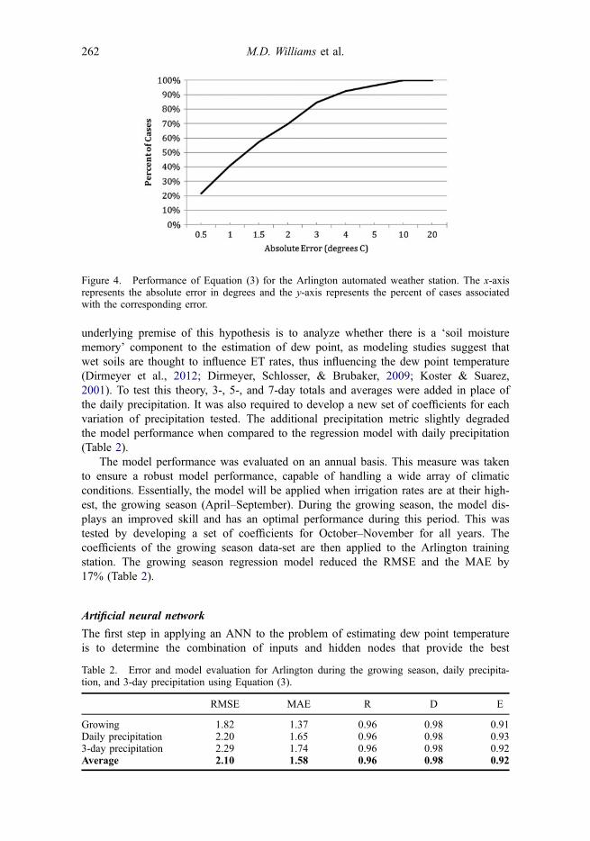
We observed some biases in the models at high and low dew points. This resultwas present in all three methods, although only Equation (3) is shown here. This iscaptured in the scatter plot of estimated vs. observed minus estimated dew point valuesfrom the Arlington automated weather station (Figure 3). Figure 3 shows a greater ten-dency for the model to underestimate values on the low end of dew point spectrum.Arlington is used as a representative station because it has the lowest RMSE and MAEfor the selected method. Other stations are expected to perform comparably to theArlington station. There is also a tendency for the overestimation of dew point at thehigh end. Even with the discrepancies mentioned above, equation three does an ade-quate job of capturing the observed variability. The overall performance of the model isadequate as well, as approximately 85% of the estimated values are within 3 °C of theobserved values (Figure 4).

Since the method that included precipitation performed best, it was a natural inquiryto see whether different variations of precipitation improved the skill of the model. The

Figure 3. Observed vs. the difference between Estimated and Observed scatter plot forArlington GEAMN station. The x-axis and y-axis are shown in degrees Celsius.

Physical Geography 261

underlying premise of this hypothesis is to analyze whether there is a ‘soil moisturememory’ component to the estimation of dew point, as modeling studies suggest thatwet soils are thought to influence ET rates, thus influencing the dew point temperature(Dirmeyer et al., 2012; Dirmeyer, Schlosser, & Brubaker, 2009; Koster & Suarez,2001). To test this theory, 3-, 5-, and 7-day totals and averages were added in place ofthe daily precipitation. It was also required to develop a new set of coefficients for eachvariation of precipitation tested. The additional precipitation metric slightly degradedthe model performance when compared to the regression model with daily precipitation(Table 2).

The model performance was evaluated on an annual basis. This measure was takento ensure a robust model performance, capable of handling a wide array of climaticconditions. Essentially, the model will be applied when irrigation rates are at their high-est, the growing season (April–September). During the growing season, the model dis-plays an improved skill and has an optimal performance during this period. This wastested by developing a set of coefficients for October–November for all years. Thecoefficients of the growing season data-set are then applied to the Arlington trainingstation. The growing season regression model reduced the RMSE and the MAE by17% (Table 2).

Artificial neural network

The first step in applying an ANN to the problem of estimating dew point temperatureis to determine the combination of inputs and hidden nodes that provide the best

Figure 4. Performance of Equation (3) for the Arlington automated weather station. The x-axisrepresents the absolute error in degrees and the y-axis represents the percent of cases associatedwith the corresponding error.

Table 2. Error and model evaluation for Arlington during the growing season, daily precipita-tion, and 3-day precipitation using Equation (3).

RMSE MAE R D E

Growing 1.82 1.37 0.96 0.98 0.91Daily precipitation 2.20 1.65 0.96 0.98 0.933-day precipitation 2.29 1.74 0.96 0.98 0.92Average 2.10 1.58 0.96 0.98 0.92

262 M.D. Williams et al.

performance. The number of inputs is dependent upon the number of days worth ofprecipitation data, we wish to include in the analysis and ranges from zero to five.Other inputs included in all networks are minimum temperature, temperature range anda constant bias neuron whose value is always equal to unity. There is no formula fordetermining the optimal number of nodes in the hidden layer of a network. It is gener-ally suggested that the number of hidden nodes should be between the number ofinputs and the number of outputs (Heaton, 2013). For this study, we will test networkswith number of hidden nodes ranging from two to the number of inputs.

Figure 5 shows how number of inputs and hidden nodes affected network perfor-mance as expressed by mean absolute and RMSEs for 27 different networks. Examin-ing the figure from left to right, the first network (3_2) relies on only minimumtemperature and temperature range to determine dew point. Addition of an additionalhidden node (3_3) allows the network to better fit the data. Addition of the currentday’s precipitation (4_2) allows for further improvement in the network performance.Expanding the network beyond four inputs and two hidden nodes did not lead to anappreciable improvement in network performance. For the remainder of the study, theANN architecture used is that of four inputs (minimum temperature, temperature range,daily precipitation, and a constant) with two hidden nodes.

Overall, the ANN outperformed the regression methods of Hubbard et al. (2003), asshown in Table 3 for the training data and Table 4 for the validation data. For allstations, the ANN displayed lower error values and was equal to or better on the otherperformance metrics as well. Direct comparison between the ANN and Equation (3)shows that, on average, the ANN reduced RMSE by 6.86% and MAE by 8.30%(Table 4). One area where the ANN offered little improvement is for low dew pointtemperatures (Figure 6). For dew points in the 20–30 °C range, the ANN has an abso-lute error within 2 °C of the observed for 90% of the cases, and 60% of the time theerror is 1 °C. However, performance for the lower end of the dew point spectrum drops

Figure 5. Performance comparison of various neural network architectures for dew pointestimation. Network architectures are given on x-axis and are defined by the number of input andhidden nodes: 3_2 represents a network with three inputs and two hidden nodes.

Physical Geography 263

off quickly. When the dew points are between 0 and 10 °C, only 50% of casesare within 2° of the observed dew point and only 24% within 1 °C. Fortunately, thegrowing season of Southwest Georgia is characterized by dew point values in the range

Table 3. Error and model evaluation statistics of the ANN for the training stations.

RMSE MAE R D E

Arlington 2.08 1.57 0.97 0.98 0.93Attapulgus 2.55 1.88 0.95 0.97 0.90Cairo 2.22 1.59 0.96 0.98 0.92Dawson 2.36 1.72 0.96 0.98 0.92Newton 2.13 1.58 0.97 0.98 0.93Sneads 2.46 1.71 0.95 0.97 0.90Tifton 2.35 1.77 0.96 0.98 0.92Average 2.31 1.69 0.96 0.98 0.92

Table 4. Comparison of RMSE and MAE for Equation (3) and the ANN for the independentstations.

Neural Network Regression Percent Improvement

RMSE MAE RMSE MAE RMSE MAE

Albany 2.70 2.01 2.90 2.21 6.85% 8.92%Cordele 2.26 1.68 2.46 1.87 8.04% 10.11%Georgetown 2.24 1.67 2.43 1.83 7.74% 8.61%Moultrie 2.25 1.67 2.35 1.72 4.24% 2.93%Sasser 2.27 1.66 2.50 1.86 9.93% 10.79%Tifton-Bowen 2.32 1.68 2.44 1.83 4.99% 8.44%Average 2.34 1.73 2.51 1.89 6.86% 8.30%

Figure 6. Performance of the ANN represented as a percentage for varying dew pointtemperature ranges. The x-axis represents the absolute error in degrees and the y-axis representsthe percent of cases for the given absolute error.

264 M.D. Williams et al.

where the ANN estimates are most accurate. Note that the ANN was not retrainedusing only growing season data as was done for the regression model.

Conclusion

The overarching goal of this study was to develop a daily dew point estimation methodadapted for Southwest Georgia, as dew point is an expression of moisture in the atmo-sphere. An estimation method is needed because of the poor availability of long-termdew point observations in the region, as data on most atmospheric humidity parametersare not as available as data on temperature. With this in mind, it was desired to makethe estimation draw from readily available temperature and precipitation observationfrom NWS COOP stations in the region. The linear regression equations developed byHubbard et al. (2003) were adapted and applied to our region of interest. Three of thefive methods used by Hubbard et al. (2003) were used here, with Equation (3) perform-ing the best from an error standpoint. On average, Equation (3) performed equal to, orbetter, in all five measures of performance for the training stations (Table 1). It wasshown that the model performs best during the growing season, when irrigation ratesare at their highest, and that additional precipitation information actually degradesmodel performance. An ANN is also employed to estimate dew point.

Seven automated weather stations from the GEAMN were selected to train andvalidate each the estimation model for each technique. On an annual basis, the ANNperformed best, only bettered by the growing season version of the regression model.A growing season only version of the ANN was not tested and is something that canbe explored in the future to see whether there is any improvement in the skill of itsestimation. Each technique tested performed adequately for the region and should beable to assist in a retroactive analysis in dew point estimation in the study region.Estimating dew point from limited meteorological variables has been successfullydemonstrated in the Great Plains region, and now in Southwest Georgia. This givesconfidence into the validity of dew point estimates derived from other variables, whichcan be applied to construct dew point climatology for data poor regions. It was alsodemonstrated that the ANN provided a better overall estimate than the regressionmethod and this result could be applicable to other regions.

A possible future application of this analysis is to study the influence of agriculturalirrigation in the region. Irrigation has increased in Southwest Georgia since the early1970s (Harrison, 2001). Irrigation is a consumptive form of water use, and most of thewater used to irrigate crops is transpired back into the atmosphere. Irrigation wets thesoil, which partitions more incoming solar radiation into latent heating, resulting inincreased near-surface dew point temperatures (Adegoke, Pielke, Eastman, Mahmood,& Hubbard, 2003; Harding & Synder, 2012). Data for atmospheric humidity, includingdew point temperature, are not as available as temperature data, thus an adequatemethod to model humidity is needed. Our work has analyzed two viable methods toestimate dew point. Now that an acceptable method has been developed to estimatedew point temperatures, we have a tool that can potentially capture possible long-termchanges in near-surface humidity caused by changes in agricultural practices. Thismethod can aid in creating a proxy data-set of long-term dew point temperatures thatwould have not otherwise been available, as first-order stations are not representative ofour area of interest.

Physical Geography 265

AcknowledgmentsWe acknowledge the support of this work by the United States Forest Service and the Depart-ment of Geography at UGA. We also thank the support staff of the GAEMN for kindly providingthe data for this study and the reviewers for their thoughtful input and feedback.

ORCID

Marcus D. Williams http://orcid.org/0000-0001-8461-2976

ReferencesAdegoke, J., Pielke, R., Eastman, J., Mahmood, R., & Hubbard, K. (2003). Impact of irrigation

on midsummer surface fluxes and temperature under dry synoptic conditions: A regionalatmospheric model study of the U.S. high plains. Monthly Weather Review, 131, 556–564.

Bentley, M., & Stallins, J. (2008). Synoptic evolution of Midwestern US extreme dew pointevents. International Journal of Climatology, 28, 1213–1225.

Changnon, D., Sandstrom, M., & Schaffer, C. (2003). Relating changes in agricultural practicesto increasing dew points in extreme Chicago heat waves. Climate Research, 24, 243–254.

Dirmeyer, P., Cash, B. A., Kinter, J., Stan, C., Jung, T., Marx, L., & Towers, P. (2012). Evidencefor enhanced land–atmosphere feedback in a warming climate. Journal of Hydrometeorology,13, 981–995.

Dirmeyer, P., Schlosser, C., & Brubaker, K. (2009). Precipitation, recycling, and land memory:An integrated analysis. Journal of Hydrometeorology, 10, 278–288.

Evans, J., & Cohen, M. (2009). Regional water resource implications of bioethanol production inthe Southeastern United States. Global Change Biology, 15, 2261–2273.

Ferguson, I., & Maxwell, R. (2011). Hydrologic and land–energy feedbacks of agricultural watermanagement practices. Environmental Research Letters, 6(6), 1–7.

Foley, J. (2005). Global consequences of land use. Science, 309, 570–574.Gaffen, D., & Ross, R. (1998). Increased summertime heat stress in the US. Nature, 396,

529–530.Harding, K., & Snyder, P. (2012). Modeling the atmospheric response to irrigation in the great

plains. Part I: General impacts on precipitation and the energy budget. Journal of Hydromete-orology, 13, 1667–1686.

Harrison, K. (2001). Agricultural trends in irrigation. Proceedings of the 2001 Georgia WaterResources Conference. Athens, GA: Institute of Ecology. The University of Georgia.

Heaton, J. (2013). Introduction to neural networks for Java (2nd ed.). Chesterfield, MO: HeatonResearch.

Hoogenboom, G. (2000). The Georgia automated environmental monitoring network. Preprints ofThe 24th Conference on Agricultural and Forest Meteorology, 24, 24–25.

Hubbard, K., Mahmood, R., & Carlson, C. (2003). Estimating daily dew point temperature forthe northern great plains using maximum and minimum temperature. Agronomy Journal, 95,323–328.

Jain, S., Nayak, P., & Sudheer, K. (2008). Models for estimating evapotranspiration usingartificial neural networks, and their physical interpretation. Hydrological Processes, 22,2225–2234.

Kimball, J., Running, S., & Nemani, R. (1997). An improved method for estimating surfacehumidity from daily minimum temperature. Agricultural and Forest Meteorology, 85, 87–98.

Koster, R., & Suarez, M. (2001). Soil moisture memory in climate models. Journal of Hydrome-teorology, 2, 558–570.

Legates, D., & McCabe Jr., G. (1999). Evaluating the use of “goodness-of-fit” measures in hydro-logic and hydroclimatic model validation. American Geophysical Union, 35, 233–241.

Lippmann, S., Fuhrmann, C., Waller, A., & Richardson, D. (2013). Ambient temperature andemergency department visits for heat-related illness in North Carolina, 2007–2008. Environ-mental Research, 124, 35–42.

Mahmood, R., Nair, U., Gameda, S., Hale, R., Carleton, A., Mcalpine, C., … Beltrán-Przekurat,A. (2014). Land cover changes and their biogeophysical effects on climate. InternationalJournal of Climatology, 1(34), 1–25.

266 M.D. Williams et al.

Marshall, C., Pielke, R., Steyaert, L., & Willard, D. (2004). The impact of anthropogenic land-cover change on the Florida Peninsula sea breezes and warm season sensible weather.Monthly Weather Review, 132, 28–52.

Pielke, R., Marland, G., Betts, R., Chase, T., Eastman, J., Niles, J., … Running, S. (2002). Theinfluence of land-use change and landscape dynamics on the climate system: Relevance toclimate-change policy beyond the radiative effect of greenhouse gases. Philosophical Trans-actions of the Royal Society A: Mathematical, Physical and Engineering Sciences, 360,1705–1719.

Ramankutty, N., Evan, A., Monfreda, C., & Foley, J. (2008). Farming the planet: 1. Geographicdistribution of global agricultural lands in the year 2000. Global Biogeochemical Cycles, 22(G1003), 1–19.

Rohli, R., & Vega, A. (2008). Climatology. Sudbury, MA: Jones and Bartlett.Rosenberg, N. (1983). Microclimate: The biological environment (2nd ed.). New York, NY:

Wiley-Interscience.Rugel, K., Jackson, C., Romeis, J., Golladay, S., Hicks, D., & Dowd, J. (2012). Effects of irriga-

tion withdrawals on streamflows in a karst environment: Lower Flint River Basin, Georgia.USA. Hydrological Processes, 26(4), 523–534.

Schaul, T., Bayer, J., Wierstra, D., Sun, Y., Felder, M., Sehnke, F., … Schmidhuber, J. (2010).PyBrain. The Journal of Machine Learning Research, 11, 743–746.

Shank, D., McClendon, R., Paz, J., & Hoogenboom, G. (2008). Ensemble artificial neural net-works for prediction of dew point temperature. Applied Artificial Intelligence, 22, 523–542.

Shepherd, J., Pierce, H., & Negri, A. (2002). Rainfall modification by major urban areas: Obser-vations from spaceborne rain radar on the TRMM satellite. Journal of Applied Meteorology,41, 689–701.

Tilman, D. (2001). Forecasting agriculturally driven global environmental change. Science, 292,281–284.

Webmaster, F. (2008, June 10). Hottest place on Earth? Retrieved June 21, 2014, from http://www.crh.noaa.gov/news/display_cmsstory.php?wfo=fgf&storyid=71074&source=2

Physical Geography 267