comparison of dichotomous and polytomousjeffwu/publications/32.pdf · comparison of dichotomous and...

Journal of Statistical Planning and Inference 14 (1986) 187-202

North-Holland

187

C O M P A R I S O N O F D I C H O T O M O U S A N D P O L Y T O M O U S

R E S P O N S E M O D E L S

Siu-Keung TSE

University of New Hampshire, Durham, Nil 03824, USA

C.F. Jeff WU

University of Wisconsin-Madison, Madison, WI 53706, USA

Received i8 March 1985; revised manuscript received 2 October 1985 Recommended by R. Bartoszynski

Abstract: In some experimental situations, it is feasible to classify the outcome of the experiment

into more than two ordered categories. To compensate for the extra effort required in the more refined classification, it is important to know whether it will lead to more efficient estimates than the binary classification. It is shown that the Fisher information for the common parameters in the more elaborate model is greater, which is further supported in a numerical study. Based on a simulation study, a similar conclusion is reached regarding the extent to which such gains are achieved in small sample situations. Some empirical results are given theoretical justification.

AMS Subject Classification: 62K99, 62N05, 62B!5.

Key words: Dichotomous quantal response; Polytomous response; Fisher information; Missing information principle; LD50; Logistic curve.

1. Introduction

In binary response experiments, the observed response is a nomial variable y ,

which takes on two possible outcomes; response O~ ( y = 1) or non-response 02 (y = 2). The experiment is characterized by assuming a response curve

F(x) = P r { y = l Ix}

where F(x) is the probability of response of an experimental subject under stimulus level x. This model is common to many areas of research. In engineering research, the stimulus levels may be the force applied to equipment or the temperature increases in a system. Then the number of brittle failures or unsuccessful perfor- mances can be recorded. In material testing, glass containers may be submitted to a drop height test. The response is 'broken' or 'not broken'. In a drug test that in- volves houseflies under exposure to a particular insecticide, the number of houseflies that are either dead or alive are observed.

0378-3758/86/$3.50 © 1986, Elsevier Science Publishers B.V. (North-Holland)

188 S.K. Tse, C.F.J. Wu / Comparison of response models

Our main interest is not in the whole response curve F but instead in estimating some of the percentiles. The 100p-th percentile LDp is defined by

F(LDp) = p, (1)

i.e., LDp is the stimulus level at which the experimental subjects would respond on the average 100p% of the time. The median of F, LD0.5, has received much atten- tion in the literature. But the extreme percentiles are often more relevant and of in- trinsic interest in practical situations.

In the aforementioned examples, the outcome of the experiment can be classified into s > 2 ordered categories, for example, according to the varying degrees of damage or moribundity. The response is then called polytomous. Our purpose is to show that the polytomous response model is more efficient in estimating percentiles, and also to identify the situations in which such gains are substantial.

Throughout the paper, we consider experiments with only one stimulus variable, since the percentile LDp is well defined only in the single variable case. In Section 2, we prove that there is a definite gain in Fisher information by using the polytomous response model for estimating the parameters and percentiles associated with the dichotomous response curve. An extensive numerical study is reported in Section 3. With the response curves taking the logistic form where F(x[fl , t/l)= [1 + e x p ( - f l x - a l ) ] -I, and under different design schemes, we compare the determinants of the Fisher information matrices for the common parameters (/~,Ctl) in the dichotomous and trichotomous response models. The gain in using the latter model is more significant if the probabilities of the categories 02 and O 3 are not negligible (Theorem 3). We also report an extensive simulation study of the small sample properties of the estimators of (/~,t21) and of the percentiles under the two models. It is found that the trichotomous response model provides more efficient estimators, especially in the case of extreme percentiles, and that the percent reduction in variance of estimating the slope is bigger than that of estimating the intercept (Theorem 4). This model deserves serious consideration if one is interested in the estimation of the extreme percentiles with a relatively small sample and the extra cost required in clearly defining and classifying the outcomes is not large. In Section 4, an example on the degree of disturbed dreams among boys is given to illustrate the application of the model.

2. Comparison of information in large samples

2.1. Dichotomous response model

Assume that k groups consisting of NI, ...,Ark subjects are tested at stimulus levels x~,x2, ... ,xk. The response Y can take one of two values. In a material testing situation, the response of the material may be 'broken' or 'not broken' . Denote these two outcomes by OI and O 2. Assume the outcome O~ has a response curve

S.K. Tse, C.F.J. Wu / Comparison of response models 189

given by the distribution function F(xlfl, al)= Pr{outcome is Ol[x} and F satis-

fies: (i) the first and second partial derivatives of F with respect to fl, al exist and

are not identically zero, (ii) F(xlfl, a) is a strictly monotone function of a and is monotonical ly in-

creasing in x, (iii) lim~_o~ F(x ] ,8, a ) = 1 and lima ~_ = F(x I ,6, a) = O. Note that in this model, Pr{outcome is 0 2 I x } = l - F ( x l ~ , a l ) . Usually the

response curve F assumes the form of a probit or logit. Other models include the angular or the rectangular distribution. Finney (1978) compares these four models and concludes that they are indistinguishable for response rates between 0.05 and 0.95. Thus, in our numerical and simulation study, we use the logistic function for the response curves al though some of the theoretical results hold more generally.

For notational convenience, define Pil = Pr{outcome is 01{xi} =F(xi[fl, Otl). I n

particular, the 100p-th percentile LDp is defined by F ( L D p ) = p . Suppose, at level xi, r;~ of the Ni subjects have outcome O~. The log-likelihood function of this model is

k

log L2 = ~ {ril log Pil +(Ni - ri))log(l -Pil)}. i=1

The Fisher information matr ix for (fl, eq) under this model is

J2 = E

-02 log L 2 -02 log L 2 OP 2 OB cga

-02 log L 2 -02 log L 2

0al z

(2)

2.2. Polytomous response model

For the dichotomous response model described above, suppose the outcome 0 2

can be further classified into a number, say s - 1, of ordered categories. For example, the category 'not broken ' in the material testing example can be classified into more ordered categories according to the different degrees of damage. For s = 3, we may define Ol = broken, (92 = partially damaged, O3 = no damage. In these cases, the response variable is an ordered categorical variable which takes s possible values. These s values are considered to be qualitative rather than quantitative in nature. Some references can be found in Aitchison and Silvey (1957), Ashford (1959) and Gurland, Lee and Dahm (1960). A general class of regression models for ordinal data is developed in McCullagh (1980). More details can be found in McCullagh and Nelder (1983).

Suppose the response o f the polytomous response model is one of the s ordered outcomes, say, 01, 02, ..., 0s. Let Y be the ordered categorical variable with assigned value i if the response is Oj, j = 1, 2, . . . , s . Assume F(x[fl, a) satisfies (i),

190 S.K. Tse, C.F.J. Wu / Comparison o f response models

(ii), (iii) in Section 2.1. An ordered polytomous quantal response model is given by

P r { Y < j l x } = F ( x l f l , aj), j = 1 , . . . , s - 1, (3)

where a l < a 2 < ' - - < a s - , . There are s - 1 response curves in this more elaborate model. We have assumed that all the response curves take the same functional form with different aj while fl is assumed to be the same. With assumption (ii) in Section 2.1, these response curves would not cross each other so that the probability of each category Oj is well defined, a fact pointed out by Gurland, Lee and Dahm (1961). Also, under this assumption, the interpretation of fl would not depend on the choice of categories. The conclusion would not be affected even when adjacent categories are pooled (McCullagh, 1980).

For notational convenience, denote Pij=F(xil,B, aj), a0=-oo and as=+oo. From (3), it follows that

P r { Y = j [ x i } = P i j - P i , j_ l, j = l , 2 , .... s.

The parameters in this model are fl, a~,..., as- ~. Define the LDp to be the stimulus level at which on the average 100p percent of the test subjects will have outcome

Or. Then, we have

F(LDp l fl, al) = P.

Therefore, the estimation of LDp depends only on the parameters fl and oq. For level xi, let ril, ..., r;~ be the numbers of subjects with outcomes O~, O2, ... , Os

respectively. The log-likelihood function of this model takes the form

k

logLs --- ~ {ril log Pil +rielog(Pi2-Pij)+ "" i=l

+ (N i - ril . . . . . ri, s - l ) l O g ( l - Pi, s - I ) } "

Denote O=(fl, al,a2, . . . , a s_ , ) r . The Fisher information matrix is

where

ds = (J6(s)), 1 <_i,j<_s,

Under some regularity conditions on F(x ] fl, a), the matrix .Is is well defined and is positive definite. Furthermore, the asymptotic distribution of the MLE/~ of 0 is N(0, j - i ) (Fahrmeir and Kaufmann, 1985).

One can partition Js into

° ! 1 t ° ! J I 2 (~1

for any m = l, 2 , . . . , s - 1 where J~',")(s) is an m × m matrix, and J~z'~')(s) an ( s - m) ×


( s - m ) matrix. In particular,

0/3 ' aa~ / 0/3 ' aa~ / '

1 J(z~)(s) = E aa i Oa.i _]2<_i,j<_s-,'

j~Z)(s)=t(2) ' , . , E ( OlOgLs Ol°gLs~ T ~2, ~ J : a/3 ' ~ I

Then the Fisher information matrix for (/3,al) is Jl~)(s) r(211"~I(2) ' -- '-'12 ~°1a22

O log L s

Cg~j )2<_j<_s-I

( s )J~(s ) .

(4)

(5)

(6)

2.3. Comparison o f the Fisher information matrices

In an (s + l)-response model, the numbers of subjects with outcomes Ol, 02 , . . . , Os+l at level xi are ril,ri2,...,ri, s+ 1 respectively. Let Ri=(Ni , ril, . . . ,ri, s+l), i = 1, 2, . . . , k, be the vectors of responses for the polytomous response model. If the outcomes Os, Os+~ are collapsed into one class, then the number of response subjects in this combined category is the sum of the corresponding ra's. Equivalently, Os and Os+~ can be viewed as missing data with only the total Os+ Os+l available. Therefore, the information available in the latter s-response model can be sum- marized by the vectors R'i=(Ni, ril,...,ri~+ri, s+l), i = l , 2 , . . . , k , i.e. each Rf is a function of Ri.

The above reformulation paves the way for proving the following theorem by using the Missing Information Principle (Orchard and Woodbury, 1972). This theorem states that the Fisher information matrix

J~St)(s + 1) - J}S2)(s + 1)J~[ ) '(s + 1) Jz(~)(s + 1)

associated with the first s parameters, namely,/3,a~, . . . ,a~_l in the (s+ 1)-response model is always greater than or equal to the Fisher information matrix Js for the parameters/3, a~, . . . , a~_ j in the s-response model. The second model is obtained by combining the last two outcomes of the first model into one group. Define A > B if A - B is non-negative definite.

Theorem 1. For s > 2,

J}~)(s + 1)- J}[)(s + l)J~[ ~ '(s + l)J~)(s + l) >_ Js. In fact,

J}Sl)(s + 1) - J}S2)(s + I) J2t[ )' ( s+ 1) J2tJ)(s + 1 ) - J s

o a21)rail = o o _ ± i ! a33 i

L a21 0 a22 [_ a32

[a31, 0 , . . . , a32]


where

a'l= XNii=, l -? i , s_ l \ -~

a21 =

+ , . . ] _ _ _

Pi, - &,- aB a#

k[ F,N, i = 1

1 -Pis OPi, s-I (l-Pi, s_l)(Pis-Pi, s_l) Off

1 (OPis'~ 2 ]

l _ Pis \-ff-~. / • 1 aP,,] oP,,s_,

Pis - Pi, s_ l - ~ j aas- i

az2 = 2 Ni i=, (1-Pi, s_l)(Pis-Pi, s_j) @as_l ~.; Ni [ 1-Pi, s-t aPis 1 aPi, s_t]aPis

a 3 1 i (Pis-Pi, s_ j ) (1-Pis ) 0t~ Pis -P~s_ l Off aas"

a32 = i=l ~ (Pis-Pi , s_l) OCt s Oas_ I "

a33= ~ Ni (Pis P i s - l ) ( 1 - P i s ) \aPi,/" i = l - - ,

All the proofs in this paper are given in the Appendix. By a similar argument, we can show that more information is gained by having

a more refined classification of other ordered responses. Therefore, although there are additional parameters to be estimated in the augmented model, there is still a

gain in information as a result of a more refined classification of the response. A result similar to Theorem 1 may also hold for other information criteria. In particular, the next result compares the Fisher information matrix associated

with the parameters (fl, a~) of any polytomous response model with that of the corresponding dichotomous response model. Based on this result, we can conclude that LDp can be estimated more efficiently by using the polytomous response model.

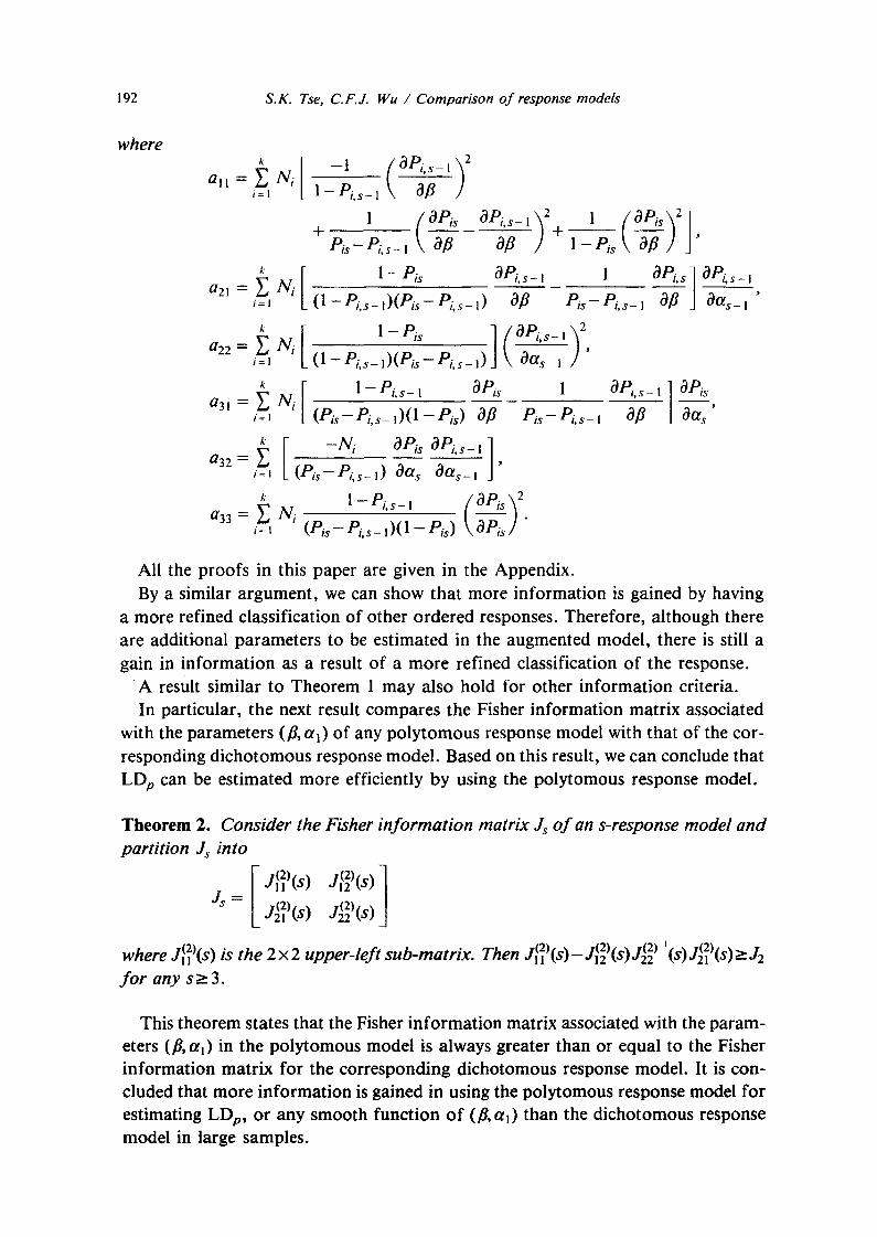
Theorem 2. Consider the Fisher information matrix Js of an s-response model and partition .Is into

L J~2)(s) J~2)(s) l Js= J ks) Jh (s)

where J~2)(s) is the 2x2 upper-left sub-matrix. Then J~Z~(s) - Jl't2)"'2 ,~J ~22"t2) '(s)j~2)(s)>_jz for any s>_ 3.

This theorem states that the Fisher information matrix associated with the parameters (fl, al) in the polytomous model is always greater than or equal to the Fisher information matrix for the corresponding dichotomous response model. It is con- cluded that more information is gained in using the polytomous response model for estimating LDp, or any smooth function of (fl, al) than the dichotomous response model in large samples.


3. Numerical study

3.1. Evaluation o f the Fisher information matrices

In this section, we perform a numerical comparison of the Fisher information matrices associated with the dichotomous response model and the polytomous response model. In particular, we assume the response curves to be logistic and s = 3. Therefore, for given stimulus level x, it follows that

P r { y = l lx } = [1 + e x p ( - f l x - a t ) ] -I,

P r { y = 2 Ix} = [1 +exp( - f l x -c t2 ) ] -I - [1 + e x p ( - f l x - a l ) ] -1, (7)

P r{y 3Ix} 1 [ l + e x p ( - f l x - -l = = -- •2)] ' 0~1 < a 2 "

The dichotomous response model is obtained by combining the second and the third categories into one group. Thus the common parameters of interest are ,6 and a~.

Without loss of generality, we assume the first response curve is given by the standard logistic curve (fl = 1, a~ = 0). Two different design patterns are chosen. Scheme I chooses the 10, 40, 60, 90 percentiles of the first response curve as design points while the 5, 45, 55, 95 percentiles are used in Scheme I1. Different values of u2 are

used. We fix the total sample size to be 40. Various numbers of observations are allocated to each percentile, the allocations varying from the balanced to the un- balanced, either skewed to the left or right. The purpose is to study the gain in informat ion under different combinations of design scheme, allocation pattern of the

subjects and the relative distance of the two response curves. In Table 1, we give the ratio of the determinants of the Fisher information

matrices for ( / / ,a j ) under the two models. The formulae are given by (1), (4), (5),

(6).

Table 1 Ratio o f the determinants o f the Fisher informat ion matrices for the 3-response and 2-response model

(fl=l, a~=0)

Design scheme a 2 = 0.1 0.5 1.0 1.5 2.0 3.0 4.0

(15,5 ,5 , 15) 1 1.04 1.18 1.29 1.32 1.28 1.15 i.06

11 1.05 i.23 1.43 1.53 ! .50 1.29 1.12

(10 ,10 ,10 ,10) 1 !.04 1.19 1.36 1.44 1.43 1.27 1.12

I I 1.05 1.25 1.53 1.77 1.87 1.62 1.29

(15, 15,5,5) 1 ! .04 1.21 1.39 1.48 1.47 1.29 !.13

II 1.06 1.32 1.67 1.94 2.01 1.67 t.31

(5,5, 15, 15) 1 1.04 1.18 1.33 1.43 1.44 1.29 1.14 [1 1.03 1.17 1.38 1.58 1.70 1.58 1.29

(5, 15, 15,5) I 1.04 1.19 1.37 1.50 1.54 1.39 1.19 I I 1.05 1.25 1.57 1.92 2.18 2. I I 1.60

Note: (15,5,5, 15) 1 means that 15,5,5, 15 observat ions are respectively assigned to the four levels o f

design scheme I.

194 S.K. Tse, C.F.J. Wu / Comparison o f response models

The two response curves are related in the following manners: (i) If a 2 is close to a~, the two curves are close to each other, i.e. the probability

that y = 2 is small and most of the responses observed are classified either as y = l

or y = 3 . (ii) If az is too large, the curve corresponding to O~ + O 2 is close to 1, i.e. the

probabili ty that y = 3 is small and the responses observed are mostly y = 1 or y = 2. In either case, one of the classes O2, O3 has few subjects. Therefore, it is not

worth the additional labor in refining the response 02 + 03 into O2 and 03. Thus, the gain in using the t r ichotomous response model in these cases would not be very significant. As we can see from the table, the ratio increases as a2 increases to 2.0 and then decreases. When a2 is sufficiently large, the corresponding ratio of the determinants of the information matrices is close to 1. These facts can be justified by the following results.

l(2)t"l~ l(2)1"1~/(2) ~(3)J~)(3)-J2 to be the gain in informa- Define dl(`8, a l ) =.,1l ~-'J - -,12 ~.--')a22 t ion in using the 3-response model, instead of the 2-response model, for estimating (`8, aj).

Theorem 3. / f the probability o f each category & given by (7), then for fixed al, Al(`8,ctl)--,O as (i) a 2 ~ a I or (ii) a2- ,oo.

The percentage gains shown in the table are at least 5% with most of them more than 15%, some up to 100%. This gives an asymptotic justification for choosing the 3-response model to estimate the parameters. We have also computed such ratios

for other design schemes. They exhibit the same pattern, and are therefore omitted. In the previous comparison we use the determinant of the Fisher information

matrix as a convenient summary criterion. A practical question is to what extent does this criterion reflect the performance of estimates of different parameters in the finite sample situations? It can only be answered by Monte Carlo simulation.

Such results, reported in the next section, support the general conclusion of this sec-

t ion in using the 3-response model, instead of the 2-response model, for estimating aO.

3.2. A simulation study

We reiterate that our main interest is in estimating the percentiles associated with the outcome O~. In this section, we present an extensive simulation study to compare the 3-response model and the 2-response model for estimating ,8, a j , LD0.1,

LD0. 3, LD0.5, LD0. 7 and LD0. 9 under different design schemes. The Fisher informa- t ion in Section 3.1 is an asymptotic measure while Table 2 presents simulation results for sample size 40. The latter results provide a more realistic indication of the performance of these estimators in small samples under the two models.

Again, we assume that the underlying response curve F ( x l ` 8, a) is logistic. The 100p-th percentile of the first response curve is given by


Table 2 Comparison of MSE of the MLE of parameters al, ,8 and the percentiles in standard logistic model with

1000 simulation samples (al =0 , ,8= 1)

Design scheme (15,5,5, 15) 1

Parameter a2 in 3-response model

0.1 0.5 !.0 1.5 2.0 3.0 4.0

2-response model

at 0.26 0.26 0.24 0.23 0.25 0.26 0.27 0.33

fl 0.15 0.15 0.11 0.10 0.11 0.15 0.18 0.64

LDo.I 0.65 0.62 0.52 0.51 0.53 0.64 0.72 0.74

LDo3 0.26 0.25 0.22 0.22 0.23 0.26 0.28 0.28

LDo.5 0.20 0.20 0.19 0.18 0.19 0.20 0.20 0.19 LDo.7 0.28 0.28 0.27 0.25 0.26 0.26 0.27 0.27

LDo.9 0.70 0.69 0.63 0.58 0.59 0.65 0.70 0.72

Design scheme (10, 10, 10, 10) 1

ct~ 0.18 0.18 0.17 0.17 0.17 0.17 0.18 0.19

fl 0.21 0.21 0.14 0.11 0.13 0.17 0.23 0.28

LDo.~ 0.96 0.81 0.62 0.63 0.64 0.76 0.86 0.99

LDtL3 0.28 0.25 0.21 0.22 0.22 0.24 0.26 0.29

LDo.5 0.17 0.15 0.15 0.16 0.15 0.16 0.16 0.16

LD0. 7 0.29 0.26 0.24 0.23 0.23 0.26 0.27 0.28 LD0.9 0.99 0.83 0.70 0.66 0.67 0.80 0.88 0.97

Design scheme (15, 15,5,5) 1

at 0.19 0.19 0.20 0.19 0~20 0.20 0.20 0.39 fl 0.23 0.19 0.16 0.13 0.14 0.16 0.27 1.72

LD0.1 0.80 0.61 0.47 0.44 0.47 0.58 0.72 0.92

LDo. 3 0.18 0.18 0.16 0.17 0.17 0.19 0.19 0.21

LDo.5 0.24 0.21 0.20 0.19 0.19 0.18 0.21 0.23

LDo.7 0.64 0.46 0.41 0.36 0.36 0.37 0.50 0.63

LDo. 9 1.98 1.33 1.12 0.94 0.94 1.06 1.51 2.02

Design scheme (5,5, 15, 15) 1

a t 0.20 0.19 0.19 0.18 0.19 0.20 0.19 0.22

,8 0.22 0.20 0.19 0.14 0.14 0.18 0.23 0.25

LDo.I 1.74 2.77 3.60 2.52 3.71 3.93 3.89 4.41

LDo. 3 0.54 0.89 1.15 0.81 1.19 1.24 1.24 1.38

LDo.5 0.21 0.31 0.38 0.29 0.39 0.40 0.40 0.43 LDo. 7 0.21 0.19 0.21 0.20 0.20 0.21 0.19 0.22

LDo. 9 0.86 0.94 1.17 0.93 1.16 1.27 1.16 1.40

Design scheme (5, 15, 15,5) 1

al 0.14 0.15 0.14 0.14 0.14 0.14 0.14 0.15 ,8 0.32 0.26 0.25 0.21 0.19 0.19 0.29 0.39 LDo.i 2.79 3.58 2.84 2.47 3.18 2.73 2.60 5.29 LD~I.3 0.57 0.83 0.67 0.60 0.76 0.63 0.60 1.20

LDo.5 0.21 0.20 0.20 0.19 0.20 0.19 0.18 0.25 LDo.7 0.65 0.42 0.43 0,37 0.38 0.42 0.42 0.55 LDo. 9 3.00 2.53 2.24 1.89 2.22 2.18 2.14 3.58

Note: The 2-response model corresponds to a2 = oo in the 3-response model.


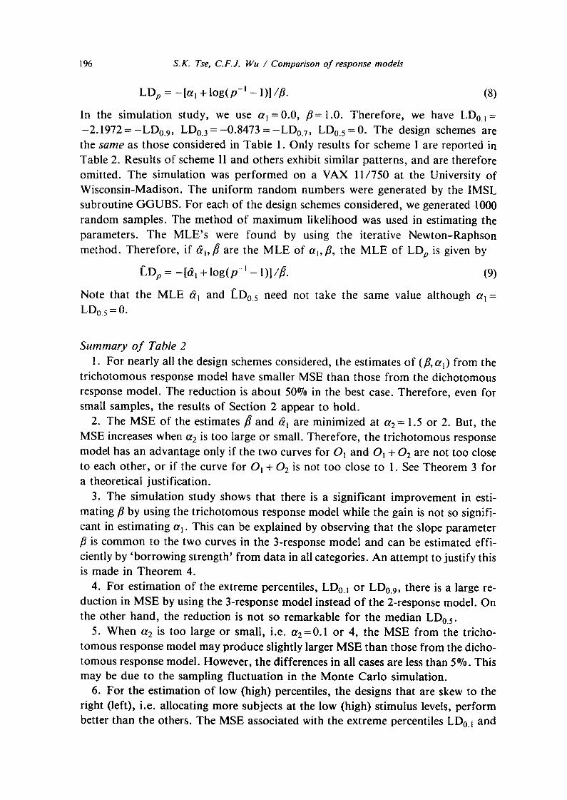
LDp = - [ u I + log(p -I - 1)]/,8. (8)

In the simulation study, we use a l = 0 . 0 , f l= 1.0. Therefore, we have LD0.1=

- 2 . 1 9 7 2 = - L D o . 9, LD0.3=-0 .8473=-LD0.7 , LD0.5=0. The design schemes are the same as those considered in Table 1. Only results for scheme I are reported in Table 2. Results of scheme II and others exhibit similar patterns, and are therefore omitted. The simulation was performed on a VAX 11/750 at the University of Wisconsin-Madison. The uniform random numbers were generated by the IMSL subroutine GGUBS. For each of the design schemes considered, we generated 1000

random samples. The method of maximum likelihood was used in estimating the parameters. The MLE's were found by using the iterative Newton-Raphson method. Therefore, if t~l,/~ are the MLE of al, fl, the MLE of LDp is given by

[~ Dp = - [t~ 1 + log ( p - i _ 1 )1//~. (9)

Note that the MLE dq and LDo. 5 need not take the same value although ct~ =

LD0. 5 = 0.

Summary o f Table 2

1. For nearly all the design schemes considered, the estimates of (fl, al) from the tr ichotomous response model have smaller MSE than those from the dichotomous response model. The reduction is about 50°70 in the best case. Therefore, even for small samples, the results of Section 2 appear to hold.

2. The MSE of the estimates/~ and ~ are minimized at a2 = 1.5 or 2. But, the MSE increases when az is too large or small. Therefore, the tr ichotomous response model has an advantage only if the two curves for O~ and O~ + O2 are not too close to each other, or if the curve for O ! + 0 2 is not too close to I. See Theorem 3 for a theoretical justification.

3. The simulation study shows that there is a significant improvement in estimating fl by using the tr ichotomous response model while the gain is not so significant in estimating a~. This can be explained by observing that the slope parameter fl is common to the two curves in the 3-response model and can be estimated efficiently by 'borrowing strength' from data in all categories. An attempt to justify this is made in Theorem 4.

4. For estimation of the extreme percentiles, LD0.j or LD0.9, there is a large reduction in MSE by using the 3-response model instead of the 2-response model. On the other hand, the reduction is not so remarkable for the median LD0. 5.

5. When ot 2 is too large or small, i.e. u 2=0.1 or 4, the MSE from the trichotomous response model may produce slightly larger MSE than those from the dichotomous response model. However, the differences in all cases are less than 5070. This may be due to the sampling f luctuat ion in the Monte Carlo simulation.

6. For the estimation of low (high) percentiles, the designs that are skew to the right (left), i.e. allocating more subjects at the low (high) stimulus levels, perform better than the others. The MSE associated with the extreme percentiles LD0. ~ and


LD0. 9 are higher than the others. This illustrates the fact that the estimates of these extreme percentiles are very unstable. In particular, the V-shaped design (i.e. more observations on the extremes) gives the smallest MSE for the extreme percentiles while those associated with the A-shaped design (i.e. fewer observations on the extremes) are the largest. However, the balanced design gives overall good performance in estimating the percentiles.

Point 3 will be further justified as follows. Let O= (B,a~) and 6= a 2 - a I • Under the 3-response model, asymptotically,

12~ t2~ (2) '(3)J2t~(3)]-I = [ 21jlJ ;talS) Cov(/~) =-- [Jll (3)-J12 (3)J22 ~2uB }taa •

Similarly, under the 2-response model,

(t" Cov(g)___- =

Theorem 4. Assume the response curves are log&tic. I f the design scheme & symmetric about the median LDo. 5 o f the first response curve, then for small ~ > O,

l"" - 2 ua 1/J/s- 2/~/1 <

laa !/11~ ,

i.e. the percent-reduction in variance o f the estimate ]] & larger than that o f dq.

A heuristic justification of point 4 follows from the above result. Let a=(-LDu/ f l , -1 / f l ) , then var(I~Do)=acov(0)a T. For extreme percentiles, (LDu/fl)Evar(fl) becomes the dominant term of var(LDp). A large percent- reduction in variance of /~ would help reduce the variance of LDR.

4. An example

The data in Table 3 are taken from Maxwell (1961, p. 70) and concern the degree of disturbed dreams among 223 boys aged 5-15. Originally, there were four categories. We combine the data so that the degree of severity of disturbed dreams of each boy is classified into three ordered and mutually exclusive classes.

Define x = - ( m i d - p o i n t of each age-category). A preliminary plot of the trans- formed variables

log( ri l+l ~ (' ril+ri2+½ \ N i - r i l + ½ J and l O g \ N i _ r i l _ r i 2 + ½ )

against x reveals approximately linear and parallel relationships. Therefore, we fit the data to the logistic model (7). The estimates are /~=0.18, t~ =0.38, 6 = 1.38. The estimated covariance matrix for (/~,t~l) is


(0.0029 0.03~ c6v(/~,t~) = \0 .03 0 .34 / "

The Pearson Z2-statistic is 5.01 with 7 degrees of freedom. Suppose we are interested in the minimum age that a boy would suffer from

severely disturbed dream for only 10°70 of the time, i.e. to estimate the 10 percentile of the response curve related to category 1. Based on the above result, we have ~D0.~0=-14.32 with S.E. =2.29, i.e. the age is 14.32.

Suppose we only rate the disturbed dreams as 'severe' or 'not severe'. Therefore, the data are obtained by combining categories 2 and 3 into one group. We fit a binary logistic curve to the combined data. The corresponding estimates are/~= 0.19 and 6'1 =0.54. The estimated covariance matrix for (fl, t~l) is

(0.0045 0.047'~ c6v(/~'al) = \0 .047 0.51 / "

The Pearson 1:2-statistics is 1.79 with 3 degrees of freedom. The estimate of the 10 percentile is f, Do.10 = -14.41 with S.E. = 2.71.

Comparing the estimates from the two models, we can see that there is about 20°-/o reduction in s tandard errors of the two estimates of p and a l . For estimation of the LD0. m, the reduction is about 15%.

5. Conclusion

Generally, our main concern is with the estimation of percentiles. The simulation study shows that in most cases considered, the MSE of L, Dp from the trichotomous response model is less than that of the dichotomous response model. Although the reductions are negligible in some cases, the majori ty of them are f rom 5°70 to 10°70, some up to 20°70. Therefore, it is worthwhile to use the t r ichotomous response model if the classification of outcomes can be defined clearly and implemented easily. Especially if one is interested in estimating the extreme percentiles and the test subjects are expensive, it would be very costly to use a relatively large sample size in order to have reliable estimates. The use of the tr ichotomous response model is a viable alternative for providing better estimates of these extreme percentiles. There- fore it should be seriously considered in practice.

Appendix

Proof of Theorem 1. Define 0 = (/~, al,... , as), R = (Rl, R2, . . . , Rk), R ' = (R~, R2, . . . , R~.) and let J(O ] R), J(O [ R') be the Fisher information matrices associated with the vectors R, R' respectively, i.e. information from the (s 4- 1)-response and s-response model.

S.K. Tse, C.F.J. Wu / Comparison o f response models 199

By the result of the general Missing Information Principle (Orchard and Woodbury, 1972), we have

J(O I R) = J(O I R')+ J(O,R' [ R) (AI)

and J(O;R'IR)>--O, which is the information lost from combining 0 s and Os+ ~ into one category. In particular, J(O [ R) is the expectation of the symmetric matrix

i -02 log Ls + ! ~Off z --0 2 log Ls + l/Off Oa 1

-0 z log Ls + 1~Off Oas

° ° °

--0 2 log Ls+ l/cgce 2 " . °

-02 log L~ + i /cga 2

= '*'12

"21"(s+1) j2(~+l)

and J(O I R') is obtained by replacing the last row and column of the above matrix by zero, i.e.

,,o,, 00) By (A1), we have J(O[R)>_J(O[R'), which is equivalent to

I J'])(s+ l ) -Js J~Sz)(s+ l) l > 0

J~])(s+ 1) Jzt~)(s+ 1)

which in turn implies J[])(s + l)-Js-JlS2)(s + 1)J2~ ) '(s + 1)Jzt])(s + 1)>_0, thus proving Theorem 1. The formulae for a 0 are easily obtained from computing

E ( - O 2 1 ° g L s + " ) and E ( - 0 2 1 ° g L s ' ] .

Proof of Theorem 2. Since

J(OIR' )=E

-021ogL2/0fl 2 --021OgL2/0flcgal 0 ""

--0 a log L2/O fl 0ct I --02 log L2/cgot 2 0

0 0 • .

0 0 -.- 0

l

0

0

0

the result follows by applying an argument similar to the above.

Proof of Theorem 3. Let Pii=[l+exp(-flxi-aj)]-I and Qij=l-Pij , j = l , 2 , i - - l , 2 .... , k. The aij defined in Theorem l are simplified as follows:

200 S.K. Tse, C.F.J. Wll/ Comparison of response models

k

tlll = ~ n ix2(P i2 -P i l )Qi lQi2 , i - I

* ni p2 Qi, Qi2 a22 = E

, P a - P ,

k r l i P i l P i 2 Q i l Q i 2 ¢123 = -- E

i=l Pi2 - Pil

k a12 = E nixiPi lQi lQi2,

i-I

k

a13 = E nixiPi2QilQi2, i=1

2 ~" niPi2QilQi2

a33 = i ~ l Pi2 - Pil

( i ) a = a2 - 61 ~ oo: The positive definiteness of J3 implies Jzt~)(3) # z ) ' (2) > • ,22 (3)J~i (3 )_0 . By Theorem I,

we have O<Al(fl, al)<_J~2)(3)-J2. As a+oo, P i2~l and Qi2+O. But

12) ( ( / I I a12"~ -Ill (3) - J2 = --, 0 a12 a22/

because Qi2 in a;j converges to O. This implies Al(fl, a l ) ~ 0 . ( i i ) 6 = a2 - al --* 0:

This implies Pi2--* Pil and Qi2 "* Qil, i = 1, 2,.. . , k. Using Taylor series expansion of Pn in a2 around a~, i.e. expansion about a = 0 , for i = 1 , 2 . . . . ,k , we have Pi2-Pil =6PnQil +hi(J) where hi(6)=0(62) which implies

Pa- Pil - 1 + 0 ( 6 ) ( A 2 )

6PilQil

where 0 ( 6 ) is a term of order 6. Consider

all - a23/a33

= X - - - i=1 " i=, i= P i 2 - Pn /

= 2 nix2(piz-Pi,)oi ,ei2 - 6 nixiPi2Qi,ei - - ' ni P22 Q il Qi2

i=l i=l PilQil[l +O(6)]/I

-+ 0 as 6--* 0, where rli,x i are fixed.

By using a similar argument , every entry of

Al(fl, al)---- I

2 - I t/I I - - a13 633

a12 - a !3 623 631

a12-a13a23a3312 -1 ]

a22 -- 023 a33

tends to zero, thus A l ( f l , a~)-- ,O.

P r o o f o f T h e o r e m 4. Recall Al(fl, al) = J{2)(3)-Jz-Jl~)(3)t(2).,22 '(3)J2t~)(3) --*0 as 6 ~ 0 . For small 6, the asymptotic covariance matrix of ( /~-f l , a l - - a l ) under the 3-response model is

[J~)(3) - .,121(2)/ax/(2),--'1.-'22 '(3) J{~)(3)] -j = [J2 + dl(fl , ct~)] -l

= J21 - J{ ldl ( f l , cq)J f I


where

J2 =

k

E nixZiPilQn E nixiPilQil i - I i=1

k k

E rlixiPilQil E niPnQil i - I i = l

L la/~ /aa

From the symmet ry o f design, la/~ = 0. Then J21 = diag(//~/~, l~,~) s o - I //j ' = l/~/~,-I la,~ =l~a-I and I a/~ = 0. Also

I -2 2 -1 J~lAl(fl, al)J~ 1 = 1~ (ajl --al3a33 )

-l -! -I l~a l ~ (a12 - a13a23a33 )

--2 iaa (a22 a23 a33 I)

Using Tay lo r series expans ion o f Pi2 in a 2 a round a I , and neglecting terms o f order higher than 6 2 ,

Pi2 = Pil + Pil Qi16 + +_62 pil Qil(Qil - Pil)+ 0(63) - (A3)

Subst i tute (A3) for ,°,2 and Qi2 in aij. With the symmetry condit ion, a f t e r some algebra , we have

k k

£/11 ~ 6 2 2 3 nixi PilQil, at3 ~ nixip2Qil , i = l i= l

1 laa, a23 = lau, a33 = + _ _ _ laa. a22 -" 6 2 4

There fore i t / t / __ ,~.t~t/

i/J/J _ ,,l/3P

lUa _ a a - 2 2 - I [I -- laa (a22 - a23 a33 )] l aa

( ~ ___~)2 62 ( l - - ~ ) 2 :-- 0(62, '

_ 2 - l i B/j [ll#3-1~(all-alaaa3 )]

laa l/3[3 I( i~_ k lliX2piiQ~l)(i~t~liPilQil ) _ ( i _~ rli xi Pi l Qi2 )2 1 .

The expression inside the bracke t is independent of 6 and is posit ive by the C a u c h y - S c h w a r z Inequal i ty , thus (IBP-2PP)/lPP=O(6). Therefore , for small 6, (l,~ _ 2 ~ ) / i ~ <_ (IPP- 2 PP)/IPP.

~mtmm v o o r W ~ . ~ , w , IntemmmMmt A ~ m ~ m ,


Acknowledgements

We thank Paul Rosenbaum for suggesting the reference Ochard and Woodbury (1972), which simplifies the original proof of Theorem I. Thanks are also due to Mike Meyer for useful comments.

This research is sponsored by the United States Army under contract No. DAAG29-80-C-0041 and by the National Foundation under grant No. MCS-8300140.

References

Aitchison, J. and S.D. Silvey (1957). The generalization of probit analysis to the case of multiple response. Biometrika 44, 131-140.

Ashford, J.R. (1959). The approach to the analysis of data for semi-quantal responses in biological assays. Biometrics 15, 573-581.

Fahrmeir, L. and H. Kaufmann (1985). Consistency and asymptotic normality of the maximum likelihood estimator in generalized linear models. Ann. Statist. 13, 342-368.

Finney, D.J. (1978). Statistical Method in Biological Assay. Hafner, New York. Gurland, J., i. Lee and P.A. Dahm (1960). Polychotomous quantal response in biological assay. Bio-

metrics 16, 382-398. Maxwell, A.E. (1961). Analysing Qualitative Data. Methuen, London. McCullagh, P. (1980). Regression models for ordinal data (with discussion). J. Roy. Statist. Soc. Ser.

B 42, 109-142. McCullagh, P. and J.A. Nelder (1983). Generalized Linear Models. Chapman and Hall, London. Orchard, T. and M.A. Woodbury (1972). A missing information principle: Theory and applications. 6th

Berkeley Syrup. Math. Statist. Prob. I, 697-715.

comparison of dichotomous and polytomousjeffwu/publications/32.pdf · comparison of dichotomous and...

Documents