comparison of frequency domain equalizers to time domain
TRANSCRIPT
LUND UNIVERSITY
PO Box 117221 00 Lund+46 46-222 00 00
Comparison of Frequency Domain Equalizers to Time Domain Equalizers in WCDMA
Yaqoob, Muhammad Atif
2009
Document Version:Publisher's PDF, also known as Version of record
Link to publication
Citation for published version (APA):Yaqoob, M. A. (2009). Comparison of Frequency Domain Equalizers to Time Domain Equalizers in WCDMA.
Total number of authors:1
General rightsUnless other specific re-use rights are stated the following general rights apply:Copyright and moral rights for the publications made accessible in the public portal are retained by the authorsand/or other copyright owners and it is a condition of accessing publications that users recognise and abide by thelegal requirements associated with these rights. • Users may download and print one copy of any publication from the public portal for the purpose of private studyor research. • You may not further distribute the material or use it for any profit-making activity or commercial gain • You may freely distribute the URL identifying the publication in the public portal
Read more about Creative commons licenses: https://creativecommons.org/licenses/Take down policyIf you believe that this document breaches copyright please contact us providing details, and we will removeaccess to the work immediately and investigate your claim.
Download date: 24. Feb. 2022
Comparison of Frequency Domain Equalizers to
Time Domain Equalizers in WCDMA
Master Thesis
Muhammad Atif Yaqoob
December 2009

ii
Dedicated to
My Parents

iii
Preface
This thesis work is performed to fulfill the requirements of Master of Science degree. All of
the thesis work has been carried out over a period of about 6 months from 01-Jun-09 to 18-
Dec-09 at system simulations group EAB/KMT/BDS, ST-Ericsson, Lund and is equivalent to
30 ECTS points. This thesis work is supervised by Elias Jonsson from ST-Ericsson and
Fredrik Tufvesson from department of Electrical and Information Technology, LTH, Sweden.
I would like to take this opportunity to express my gratitude to Fredrik Tufvesson who has
shown very kind support and guidance as my masters program coordinator at LTH as well as
my thesis supervisor. I would like to extend my special thanks to Elias Jonsson for all the
technical support and encouragement throughout the period of my thesis work at ST-
Ericsson. He remained very kind and supportive during all the time. The frequent discussions
I had with him to understand different technical details of the thesis helped me achieve my set
objectives timely and effectively. I am also thankful to him for his valuable comments and
suggestions for writing this thesis report. Also, I would like to thank my Development
Manager Anders Ericsson G for providing me the opportunity to pursue a master thesis in his
group.
Finally, I would like to thank to all my friends for their enduring support and encouragement.
And to my family for their unconditional love and support during all the time I was involved
with my studies. Without their support and encouragement, this work would not be possible.
iv
Abstract
Future mobile platforms will contain an increased amount of wireless technologies. As
technologies mature it will be necessary to find synergies between them. This could be in the
form of reusing hardware blocks and algorithms. By using Fast Fourier Transforms
(FFT/IFFT) and performing channel cancellation/equalization in frequency domain for
wideband code division multiple access (WCDMA) will provide us a platform which can
support LTE and WiFi together with WCDMA. In this thesis, an equalizer based on Fast
Fourier Transforming (FFT) the input signal, cancelling the propagation channel in frequency
domain, and finally reverting to time domain using an IFFT would be devised for WCDMA.
The performance of frequency domain equalizer is then compared with traditional time
domain equalizer based on G-RAKE method for different performance metrics.
To evaluate and compare the performance of frequency domain equalizer (FFT) with time
domain equalizer (G-RAKE), a simulator is made in IT++. Several simulations are performed
and the obtained results are analyzed in Matlab. Firstly, for channel estimation at the receiver,
common pilot channel (CPICH) is used and multiple channel estimates are obtained to get a
filtered channel estimate. Along-with CPICH pilot symbols, data symbols of a desired user
and four other user‟s data symbols are transmitted from the base-station (Node B). Using
QPSK signaling, un-coded bit-error-rate (BER) results of the desired data user are compared
for the two equalization methods. Simulation results are obtained for single path and multi-
path propagation channels with different delay spread values. Included in the modeling are
one receive and transmit antenna, other cell interference, i.e., non-white noise, frequency
errors at mobile station (UE), and analog-to-digital (A/D) quantization.
v
Table of Contents
Preface ................................................................................................................................ iii
Abstract .............................................................................................................................. iv
Table of Contents ................................................................................................................ v
List of Figures................................................................................................................... viii
List of Tables ...................................................................................................................... ix
List of Abbreviations ........................................................................................................... x
1 Introduction to Project ................................................................................................ 1
1.1 Background ........................................................................................................................ 1
1.2 Motivation ......................................................................................................................... 1
1.3 Previous Work ................................................................................................................... 1
1.4 Problem Statement ............................................................................................................. 2
1.5 Contribution ....................................................................................................................... 2
2 WCDMA Overview ...................................................................................................... 4
2.1 WCDMA: An Air Interface for UMTS ............................................................................... 4
2.2 UMTS System Requirements ............................................................................................. 4
2.3 WCDMA: Main System Parameters ................................................................................... 5
2.4 Time Units ......................................................................................................................... 5
2.5 Channels ............................................................................................................................ 5
2.6 Spreading and modulation .................................................................................................. 6
2.6.1 Channelization code ................................................................................................................... 6
2.6.2 Scrambling code ......................................................................................................................... 8
2.6.3 Spreading and Transmission over the Air .................................................................................... 9
2.7 Common Pilot Channel (CPICH) ..................................................................................... 11
2.8 Example Using WCDMA ................................................................................................. 12
2.8.1 Propagation Channel Delay Time Estimation ............................................................................ 13
2.8.2 Detection of Propagation Channel Constant .............................................................................. 14
2.8.3 Data Demodulation of the Sent Data ......................................................................................... 14 2.8.3.1 RAKE ............................................................................................................................... 15 2.8.3.2 Channel Estimation ........................................................................................................... 16 2.8.3.3 Interference Estimation ..................................................................................................... 16 2.8.3.4 Signal-to-Interference Ratio (SIR) ..................................................................................... 16 2.8.3.5 Combiner .......................................................................................................................... 17
3 Equalizer Model ......................................................................................................... 18
vi
3.1 Communication System Diagram ..................................................................................... 18
3.2 RAKE (Time domain) ...................................................................................................... 18
3.2.1 Non-parametric MMSE-based Equalization .............................................................................. 19
3.2.2 ML-based Equalization (Non-parametric G-RAKE) .................................................................. 20
3.2.3 SIR........................................................................................................................................... 22
3.3 FFT (Frequency domain) .................................................................................................. 23
3.3.1 System Model .......................................................................................................................... 23
3.3.2 Demodulation ........................................................................................................................... 24
3.3.3 Approximations to investigate ................................................................................................... 26
3.3.4 Interference Calculation ............................................................................................................ 26
3.3.5 Power Calculation .................................................................................................................... 27
3.3.6 Calculation of Filtered Channel Estimate .................................................................................. 27
Chapter 4 ........................................................................................................................... 28
4 Implementation and Results ...................................................................................... 28
4.1 Simulation Setup .............................................................................................................. 28
4.1.1 Transmit Signal from Node B ................................................................................................... 29
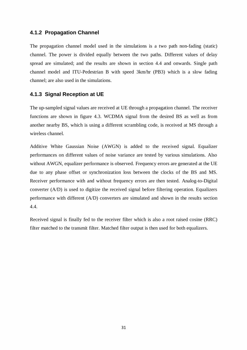
4.1.2 Propagation Channel................................................................................................................. 31
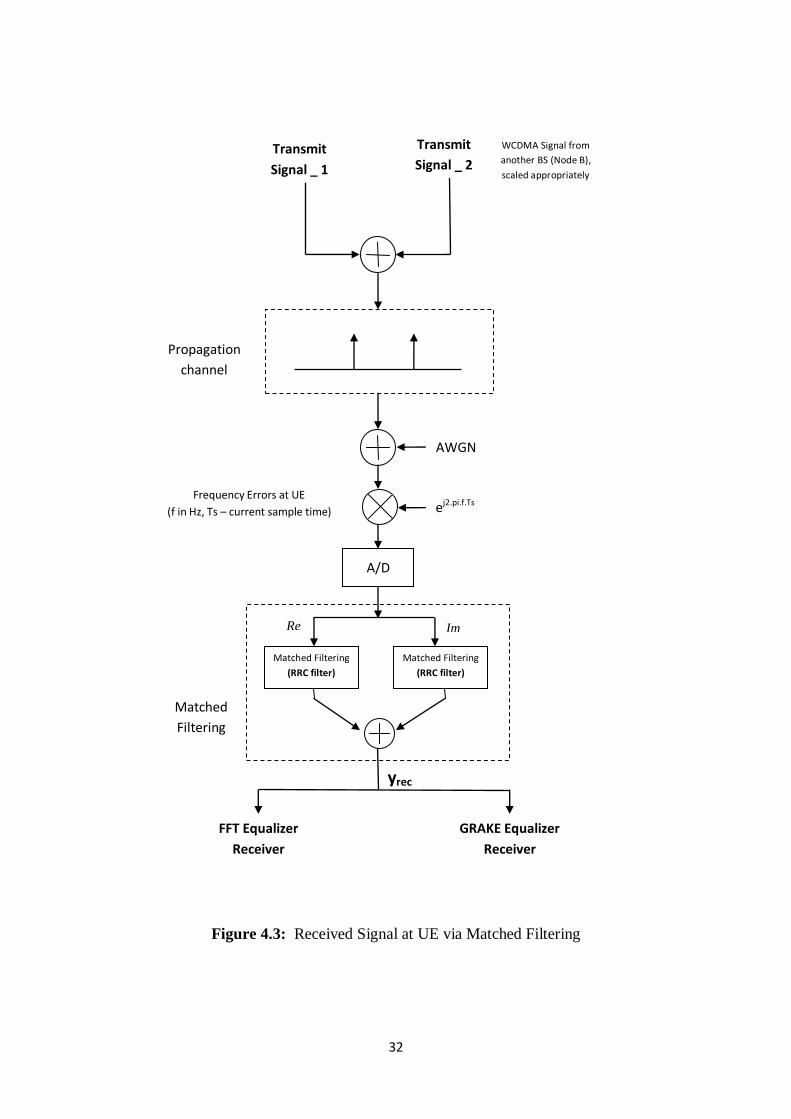
4.1.3 Signal Reception at UE ............................................................................................................. 31
4.2 GRAKE Equalizer Receiver ............................................................................................. 33
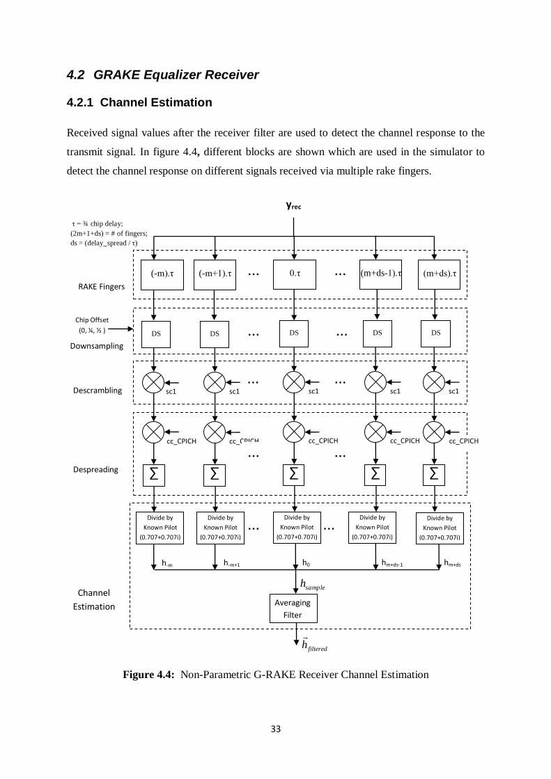
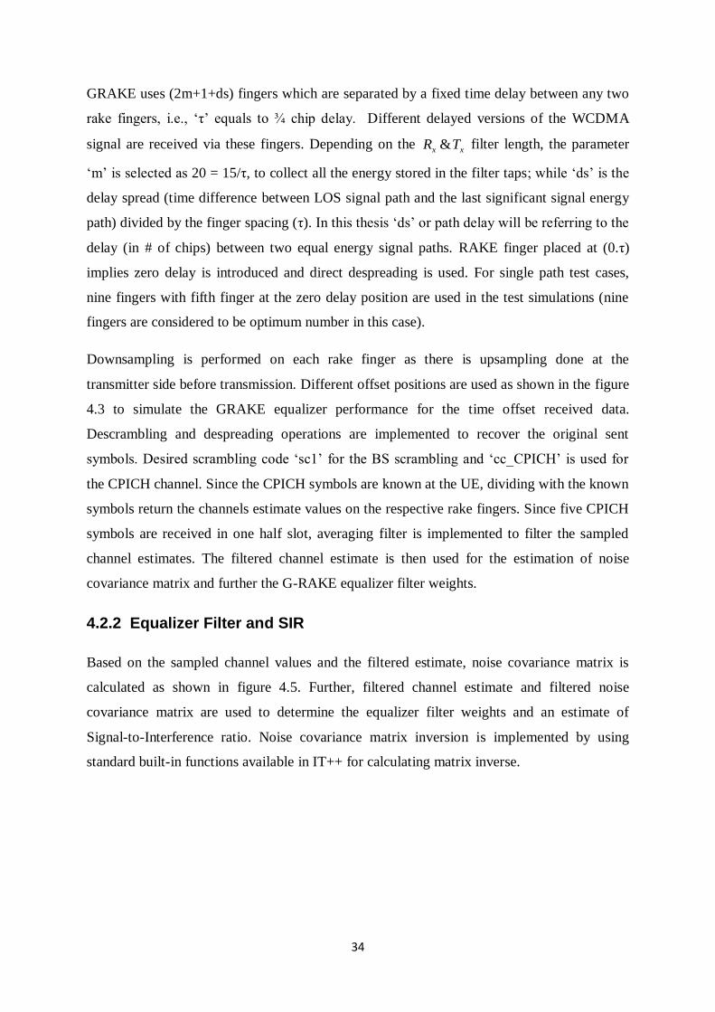
4.2.1 Channel Estimation .................................................................................................................. 33
4.2.2 Equalizer Filter and SIR............................................................................................................ 34
4.2.3 Combiner ................................................................................................................................. 35
4.3 FFT Equalizer Receiver .................................................................................................... 37
4.3.1 Channel Estimation .................................................................................................................. 37
4.3.2 Equalizer .................................................................................................................................. 38
4.3.3 Despreader Output, BER, and SIR Estimate .............................................................................. 39
4.4 Results and Discussion ..................................................................................................... 41
4.4.1 Parameters Optimization ........................................................................................................... 41 4.4.1.1 GRAKE Parameters Optimization ..................................................................................... 41 4.4.1.2 FFT Parameters Optimization ............................................................................................ 41
4.4.2 Chip Offset Comparison ........................................................................................................... 44
4.4.3 Frequency Error Comparison .................................................................................................... 51
4.4.4 Colored Noise Comparison ....................................................................................................... 54
4.4.5 Analog-to-Digital Converter Comparison .................................................................................. 55
4.4.6 Complexity Comparison ........................................................................................................... 57 4.4.6.1 FFT Equalizer Output Samples .......................................................................................... 57 4.4.6.2 Computations For FFT ...................................................................................................... 58 4.4.6.3 Computations for NP-GRAKE .......................................................................................... 59
4.4.7 ITU-Pedestrian B Channel Comparison ..................................................................................... 61
5 Conclusion .................................................................................................................. 63
vii
Appendix ........................................................................................................................... 65
A. Parametric Equalizer ............................................................................................................... 65
B. Differentiate 2
eHg w.r.t g ............................................................................................... 67
References.......................................................................................................................... 69
viii
List of Figures
Figure 2.1: OVSF code tree................................................................................................................ 8
Figure 2.2: Relationship between Spreading and Scrambling............................................................. 8
Figure 2.3: Multi-path propagation channel .................................................................................... 10
Figure 2.4: Frame structure and modulation pattern for Common Pilot Channel ............................. 11
Figure 2.5: Propagation channel estimates ..................................................................................... 14
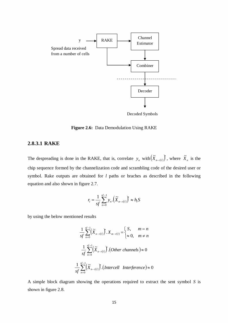
Figure 2.6: Data Demodulation Using RAKE ..................................................................................... 15
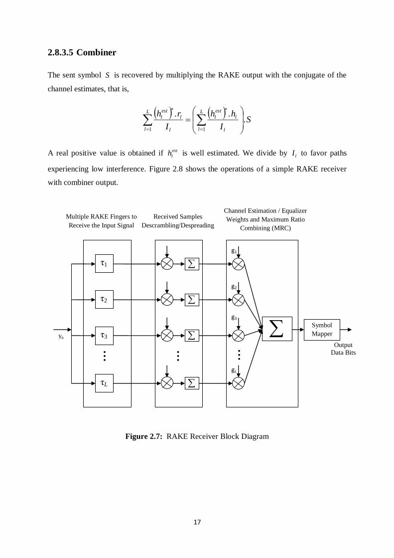
Figure 2.7: RAKE Receiver Block Diagram ........................................................................................ 17
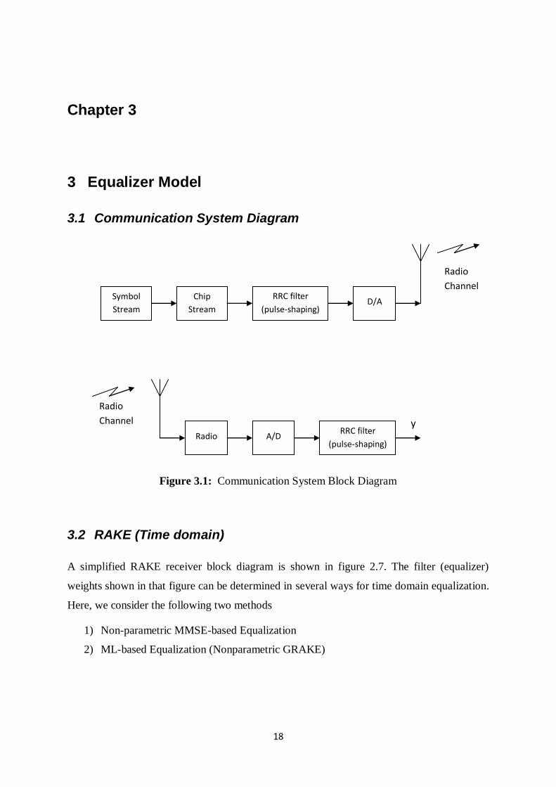
Figure 3.1: Communication System Block Diagram .......................................................................... 18
Figure 3.2: FFT Equalizer Receiver Block Diagram ............................................................................ 24
Figure 4.1: Root Raised Cosine Filter; sample rate = 4 per chip, filter length = 14chips .................... 29
Figure 4.2: Transmission of WCDMA signal from Node B................................................................. 30
Figure 4.3: Received Signal at UE via Matched Filtering ................................................................... 32
Figure 4.4: Non-Parametric G-RAKE Receiver Channel Estimation ................................................... 33
Figure 4.5: Non-Parametric G-RAKE Equalizer Filter and SIR ............................................................ 35
Figure 4.6: Non-Parametric G-RAKE Combiner Output and BER....................................................... 36
Figure 4.7: FFT Receiver Channel Estimation ................................................................................... 37
Figure 4.8: FFT Equalizer Input/Output Block Diagram .................................................................... 39
Figure 4.9: FFT Despreader Output, BER, and SIR Estimate .............................................................. 40
Figure 4.10: FFT Equalizer Output Chip Samples vs Delay Spread .................................................... 57
Figure 4.11: BER vs EcIor for FFT and GRAKE equalizer using ........................................................... 61
ix
List of Tables
Table 2.1: Main WCDMA parameters ................................................................................................ 5
Table 2.2: WCDMA Downlink Data Rate vs Spreading Factor ............................................................. 7
Table 4.1: Simulation setup: different users/channels with their sf and power assigned ................. 28
Table 4.2: NFFT vs BER for two path channel, ‘ds’ = 5 chip, h = 1/200, without AWGN .................... 43
Table 4.3: FFT Equalizer BER results for different delay spread values, NFFT = 2048, without AWGN,
h = 1/200, ...................................................................................................................................... 44
Table 4.4: Chip Offset Comparison: Single Path Channel ................................................................. 45
Table 4.5: FFT equalizer BER vs ε, IorIoc = 6 dB, two path channel ‘ds’ = 0.75 chip .......................... 46
Table 4.6: Chip Offset Comparison: Two Path Channel ‘ds’ = 0.75 Chip ........................................... 47
Table 4.7: FFT equalizer BER results at different offset positions using IorIoc = 8 dB ....................... 47
Table 4.8: Chip Offset Comparison: Two Path Channel ‘ds’ = 1 Chip ................................................ 48
Table 4.9: Chip Offset Comparison: Two Path Channel ‘ds’ = 4.5 Chip ............................................. 49
Table 4.10: Chip Offset Comparison: Two Path Channel ‘ds’ = 5 Chip .............................................. 50
Table 4.11: Frequency Error Comparison: Single Path Channel, Offset = 0 Chip ............................... 51
Table 4.12: Frequency Error Comparison: Single Path Channel, Offset = 1/2 Chip............................ 52
Table 4.13: Frequency Error Comparison: Two Path Channel ‘ds’ = 5 Chip, Offset = 0 Chip .............. 53
Table 4.14: Colored Noise Comparison ........................................................................................... 54
Table 4.15: A/D Conversion Comparison: Single Path, Offset = 0 Chip ............................................. 55
Table 4.16: A/D Conversion Comparison: Single Path, Offset = 1/2 Chip .......................................... 55
Table 4.17: A/D Conversion Comparison: Two Path ‘ds’ = 5 Chip, Offset = 0 Chip ............................ 56
Table 4.18: Complexity Comparison between FFT and G-RAKE ........................................................ 60
x
List of Abbreviations
2G 2nd
Generation Mobile Systems
3G 3rd
Generation Mobile Systems
3GPP 3rd Generation Partnership Project
A/D Analog-to-Digital Converter
AWGN Additive White Gaussian Noise
BER Bit Error Ratio
BLER Block Error Ratio
BS Base Station (Node B for UMTS)
CDMA Code Division Multiple Access
CPICH Common Pilot Channel
D/A Digital-to-Analog Converter
DS-CDMA Direct Sequence - CDMA
EcIor The chip power transmitted from Node B
EDGE Enhanced Data Rates for GSM Evolution
ETSI European Telecommunications Standards Institute
FDD Frequency Division Duplex
FDE Frequency Domain Equalization
FFT Fast Fourier Transform
GPRS General Packet Radio Service
IFFT Inverse Fast Fourier Transform
IMT-2000 International Mobile Telecommunication – 2000
ISI Inter Symbol Interference
ITU International Telecommunication Union
Ior The total transmit power from Node B (normalized to one)
Ioc Other-cell interference (including radio noise)
IorIoc Amount of inter-cell interference
LOS Line of sight
MAI Multiple Access Interference
ML Maximum Likelihood
MMSE Minimum Mean Square Error
xi
MRC Maximum Ratio Combining
MS Mobile Station (UE for UMTS)
NFFT FFT window size
NP-GRAKE Non-parametric Generalized RAKE
PN Pseudo-Noise
QPSK Quadrature Phase Shift Keying
RRC Root Raised Cosine
SIR Signal to Interference Ratio
UMTS Universal Mobile Telecommunication System
UE User Equipment
WCDMA Wideband Code Division Multiple Access
ds delay spread
os over sampling
pdf probability distribution function
sf Spreading Factor
w.r.t with respect to
1
Chapter 1
1 Introduction to Project
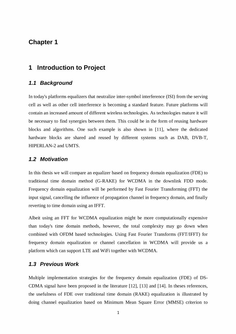
1.1 Background
In today's platforms equalizers that neutralize inter-symbol interference (ISI) from the serving
cell as well as other cell interference is becoming a standard feature. Future platforms will
contain an increased amount of different wireless technologies. As technologies mature it will
be necessary to find synergies between them. This could be in the form of reusing hardware
blocks and algorithms. One such example is also shown in [11], where the dedicated
hardware blocks are shared and reused by different systems such as DAB, DVB-T,
HIPERLAN-2 and UMTS.
1.2 Motivation
In this thesis we will compare an equalizer based on frequency domain equalization (FDE) to
traditional time domain method (G-RAKE) for WCDMA in the downlink FDD mode.
Frequency domain equalization will be performed by Fast Fourier Transforming (FFT) the
input signal, cancelling the influence of propagation channel in frequency domain, and finally
reverting to time domain using an IFFT.
Albeit using an FFT for WCDMA equalization might be more computationally expensive
than today's time domain methods, however, the total complexity may go down when
combined with OFDM based technologies. Using Fast Fourier Transforms (FFT/IFFT) for
frequency domain equalization or channel cancellation in WCDMA will provide us a
platform which can support LTE and WiFi together with WCDMA.
1.3 Previous Work
Multiple implementation strategies for the frequency domain equalization (FDE) of DS-
CDMA signal have been proposed in the literature [12], [13] and [14]. In theses references,
the usefulness of FDE over traditional time domain (RAKE) equalization is illustrated by
doing channel equalization based on Minimum Mean Square Error (MMSE) criterion to
2
combat multiple-access interference (MAI) and inter-symbol interference (ISI) and having
the same or lesser complexity requirements as well. Also [16] demonstrated that MMSE
based equalizer has better BER performance as compared to zero-forcing (ZF) and RAKE
equalizer in downlink CDMA.
Moreover, it is proposed that frequency domain equalization combined with single carrier
modulation has comparable performance results as of OFDM system having nearly the same
complexity requirements [15].
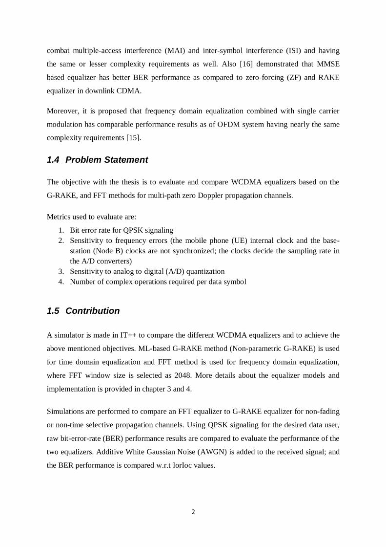
1.4 Problem Statement
The objective with the thesis is to evaluate and compare WCDMA equalizers based on the
G-RAKE, and FFT methods for multi-path zero Doppler propagation channels.
Metrics used to evaluate are:
1. Bit error rate for QPSK signaling
2. Sensitivity to frequency errors (the mobile phone (UE) internal clock and the base-
station (Node B) clocks are not synchronized; the clocks decide the sampling rate in
the A/D converters)
3. Sensitivity to analog to digital (A/D) quantization
4. Number of complex operations required per data symbol
1.5 Contribution
A simulator is made in IT++ to compare the different WCDMA equalizers and to achieve the
above mentioned objectives. ML-based G-RAKE method (Non-parametric G-RAKE) is used
for time domain equalization and FFT method is used for frequency domain equalization,
where FFT window size is selected as 2048. More details about the equalizer models and
implementation is provided in chapter 3 and 4.
Simulations are performed to compare an FFT equalizer to G-RAKE equalizer for non-fading
or non-time selective propagation channels. Using QPSK signaling for the desired data user,
raw bit-error-rate (BER) performance results are compared to evaluate the performance of the
two equalizers. Additive White Gaussian Noise (AWGN) is added to the received signal; and
the BER performance is compared w.r.t IorIoc values.
3
By using a tuned parameter „ε‟ which represents the noise variance, simulations are
performed to estimate the best expected performance of the FFT based equalizer for various
channel conditions. Optimum values of „ε‟ used in the simulations are estimated by observing
the un-coded BER performance results. Simulation results are shown in section 4.4 and
onwards.
Furthermore, different frequency errors (5, 10, 20 Hz) are generated at the mobile-station
(UE) to simulate the synchronization mismatch between the clocks of UE and Node B, and
BER performance of the two equalizer methods is compared. Non-white noise, i.e.,
interference from another Node B is added to the desired signal with appropriate scaling and
BER performance results are evaluated using the two equalization methods. Also analog-to-
digital quantization results for different (8, 10, and 12-bit) fixed point implementations with
appropriate A/D-constant (K) values used to scale the signal for integer representation, are
observed. After the simulation results, a basic complexity comparison is made in terms of
total complex operations required per data symbol using G-RAKE and FFT method based on
the algorithms used for FFT/IFFT and for other matrix operations. Conclusion and possible
future work for the FFT based equalization method is given in Chapter 5.
4
Chapter 2
2 WCDMA Overview
2.1 WCDMA: An Air Interface for UMTS
The success of second-generation (2G) cell phones, especially the Global System for Mobile
communications (GSM), motivated the development of a successor system [1]. The 2G
systems provided not only voice traffic on mobile phones but also some basic data services,
e.g., the short message service (sms). But these data services are limited to use as higher data
rates are not available which eventually limits the use of mobile phones for high quality
multimedia services.
Under the name of IMT-2000, International Telecommunication Union (ITU) asked for
proposals to standardize the work of third-generation (3G) mobile telecommunication
systems. A standard has been formulated by 3GPP, which is a joint venture of several
standard developing organizations from different regions of the world (Europe, Japan, Korea,
USA, and China).
2.2 UMTS System Requirements
The requirements for the third-generation systems are given as under [3]:
Bit rates up to 2 Mbps;
Variable bit rate to offer bandwidth on demand;
Multiplexing of services with different quality requirements on a single connection,
e.g. speech, video and packet data;
Co-existence of second and third generation systems and inter-system handovers for
coverage enhancements and load balancing;
High spectrum efficiency.
5
2.3 WCDMA: Main System Parameters
In the standardization forums, WCMDA technology has emerged as the most widely adopted
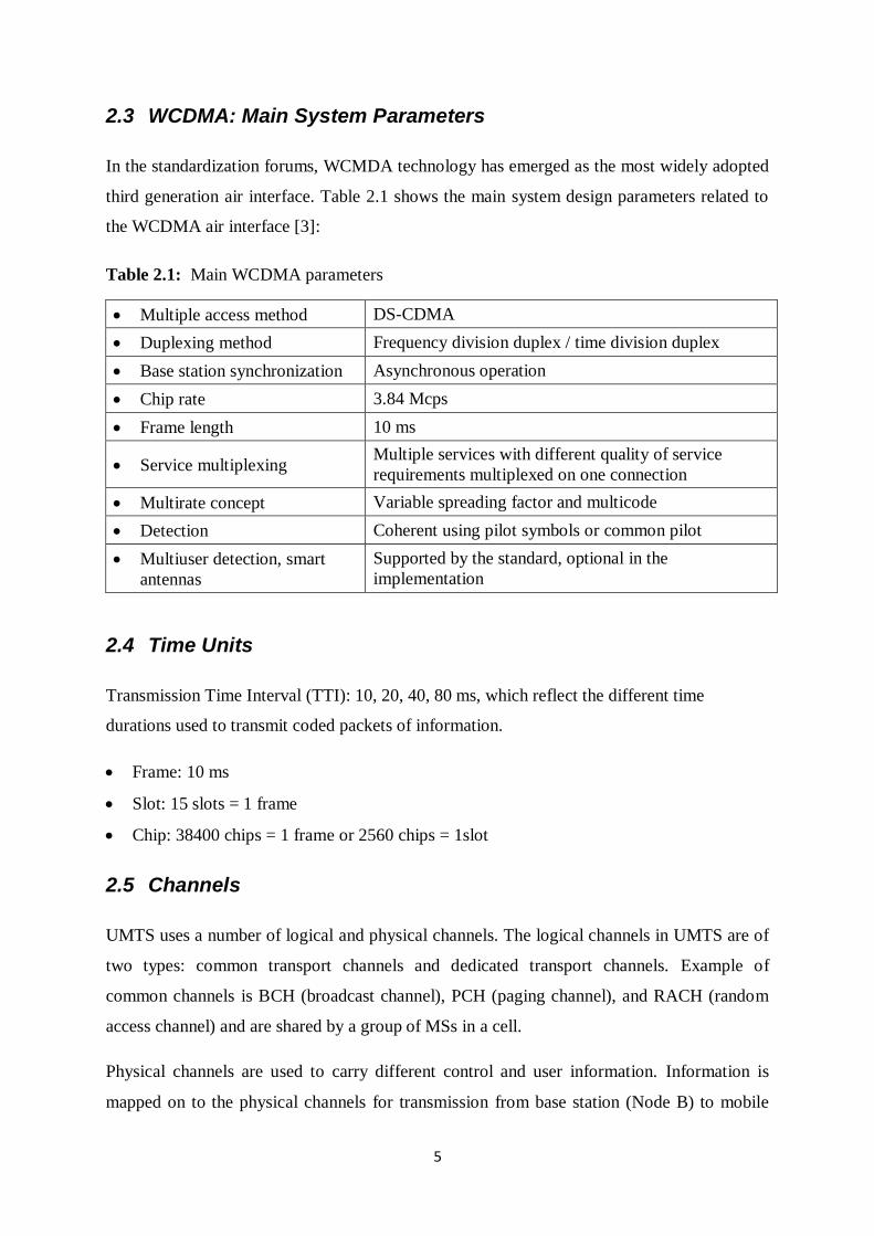
third generation air interface. Table 2.1 shows the main system design parameters related to
the WCDMA air interface [3]:
Table 2.1: Main WCDMA parameters
Multiple access method DS-CDMA
Duplexing method Frequency division duplex / time division duplex
Base station synchronization Asynchronous operation
Chip rate 3.84 Mcps
Frame length 10 ms
Service multiplexing Multiple services with different quality of service
requirements multiplexed on one connection
Multirate concept Variable spreading factor and multicode
Detection Coherent using pilot symbols or common pilot
Multiuser detection, smart
antennas
Supported by the standard, optional in the
implementation
2.4 Time Units
Transmission Time Interval (TTI): 10, 20, 40, 80 ms, which reflect the different time
durations used to transmit coded packets of information.
Frame: 10 ms
Slot: 15 slots = 1 frame
Chip: 38400 chips = 1 frame or 2560 chips = 1slot
2.5 Channels
UMTS uses a number of logical and physical channels. The logical channels in UMTS are of
two types: common transport channels and dedicated transport channels. Example of
common channels is BCH (broadcast channel), PCH (paging channel), and RACH (random
access channel) and are shared by a group of MSs in a cell.
Physical channels are used to carry different control and user information. Information is
mapped on to the physical channels for transmission from base station (Node B) to mobile
6
station (MS) or vice versa. A physical channel that is used for data and control signaling in
WCDMA is known as dedicated physical data channel (DPDCH) and is used for both uplink
and downlink transmission. Common pilot channel (CPICH) is a downlink physical channel
used to transmit known pilot symbols for channel estimation at UE and is discussed in more
detail in section 2.5. Details about other different channels used in WCDMA can be found in
the standard and also in literature [3], and [4].
2.6 Spreading and modulation
Direct-Sequence code division multiple-access (DS-CDMA) is employed in WCDMA.
Different users are assigned different codes (in the form of chips) derived from CDMA.
Codes are used to separate different users, and also they distinguish between users and other
control channels. Two types of codes: channelization codes and scrambling codes are used to
spread the user information and to assign identification tag to the different users. Basic theory
about CDMA is described in the references [5], [6], and [7].
2.6.1 Channelization code
Orthogonal channelization codes are used in WCDMA. Let nC be a vector of length 4, 8, 16,
32, 64, 128, or 256. The length of the vector is called the spreading factor sf . And a
channelization code is characterized by
mn
mnsfCC
sf
i
m
i
n
i,0
,.
1
where each element of nC equals 1 , and mn CC , are two channelization codes.
Orthogonal variable spreading factor (OVSF) code tree is used in WCDMA to assign the
channelization codes to different users. Depending on the user‟s data rate, code is assigned to
the user from the code tree. Where a short code implies high data rate and long code is used
for low data rate user. WCDMA downlink data rates (modulation scheme: QPSK) w.r.t the
spreading factor used are listed in table 2.2.
7
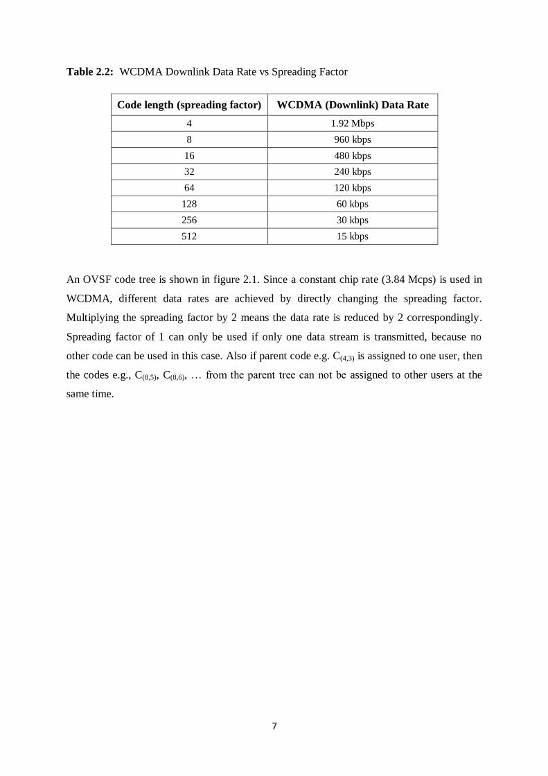
Table 2.2: WCDMA Downlink Data Rate vs Spreading Factor
Code length (spreading factor) WCDMA (Downlink) Data Rate
4 1.92 Mbps
8 960 kbps
16 480 kbps
32 240 kbps
64 120 kbps
128 60 kbps
256 30 kbps
512 15 kbps
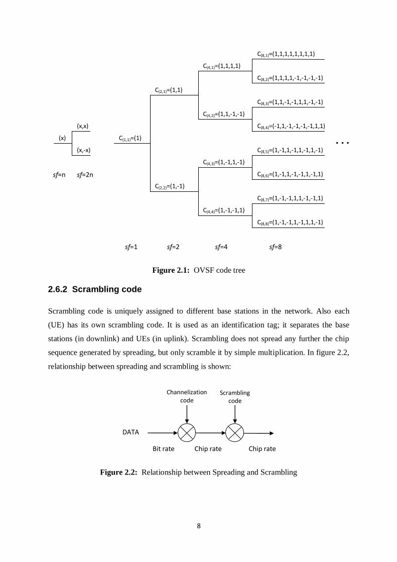
An OVSF code tree is shown in figure 2.1. Since a constant chip rate (3.84 Mcps) is used in
WCDMA, different data rates are achieved by directly changing the spreading factor.
Multiplying the spreading factor by 2 means the data rate is reduced by 2 correspondingly.
Spreading factor of 1 can only be used if only one data stream is transmitted, because no
other code can be used in this case. Also if parent code e.g. C(4,3) is assigned to one user, then
the codes e.g., C(8,5), C(8,6), … from the parent tree can not be assigned to other users at the
same time.
8
Figure 2.1: OVSF code tree
2.6.2 Scrambling code
Scrambling code is uniquely assigned to different base stations in the network. Also each
(UE) has its own scrambling code. It is used as an identification tag; it separates the base
stations (in downlink) and UEs (in uplink). Scrambling does not spread any further the chip
sequence generated by spreading, but only scramble it by simple multiplication. In figure 2.2,
relationship between spreading and scrambling is shown:
Figure 2.2: Relationship between Spreading and Scrambling
(x)
(x,-x)
(x,x)
C(1,1)=(1)
C(2,2)=(1,-1)
C(2,1)=(1,1)
C(4,4)=(1,-1,-1,1)
C(4,3)=(1,-1,1,-1)
C(4,2)=(1,1,-1,-1)
C(4,1)=(1,1,1,1)
C(8,8)=(1,-1,-1,1,-1,1,1,-1)
C(8,7)=(1,-1,-1,1,1,-1,-1,1)
C(8,6)=(1,-1,1,-1,-1,1,-1,1)
C(8,5)=(1,-1,1,-1,1,-1,1,-1)
C(8,4)=(-1,1,-1,-1,-1,-1,1,1)
C(8,3)=(1,1,-1,-1,1,1,-1,-1)
C(8,2)=(1,1,1,1,-1,-1,-1,-1)
C(8,1)=(1,1,1,1,1,1,1,1)
. . .
sf=1 sf=2 sf=4 sf=8
sf=n sf=2n
Scrambling code
Channelization code
DATA
Bit rate Chip rate Chip rate
9
They are quasi-orthogonal random sequences; e.g., a scrambling code is a vector nq of
length 38400, where each vector entry of nq is a complex number of type 21 i . The
scrambling code is constructed to approximate a random sequence, that is,
,
0,0
0,1.
38400
138400mod
38399
0
m
mqq n
mi
i
n
i
observe that if 0m the correlation is not equal to zero, but almost.
2.6.3 Spreading and Transmission over the Air
Let nS denote the symbols to be sent. Spread the symbols nS using the channelization code
C , that is,
,,,, 21 sfnnnn CSCSCSS
then multiply each spread term with the cell specific scrambling code q ,
,,,, 2211 sfsfnnn qCSqCSqCS
If 1nS is the next symbol to be transmitted, we get similarly, first by spreading
,,,, 121111 sfnnnn CSCSCSS
and afterwards by scrambling
sfsfnsfnsfn qCSqCSqCS 21221111 ,,,
Observe that the channelization code is reused for each new symbol, but the scrambling code
vector continues to be read until we reach the end of it. When the end of the scrambling code
has been reached, we start reading it from the beginning.
The purpose of the channelization codes is for the cell to be able to transmit simultaneously
several symbols to different UEs.
We have that at any given time a “CHIP” of the type nkji XqCS which needs to be
transmitted.
Alternatively, the above operation can be described as:
10
Symbols Spreading Scrambling Transmit
Propagation Channel Distortion UE-reception
Also, pulse shaping is applied on the generated chips before transmission. In WCDMA,
standard root raised cosine (rrc) pulse shape filter is used at the transmitter and matched filter
with the same filter is performed at the receiver. More details about the pulse shape filter
used is given section 4.1.1.
The sent nX are affected by the propagation channel. The propagation channel will change
the amplitude and phase of the chips.
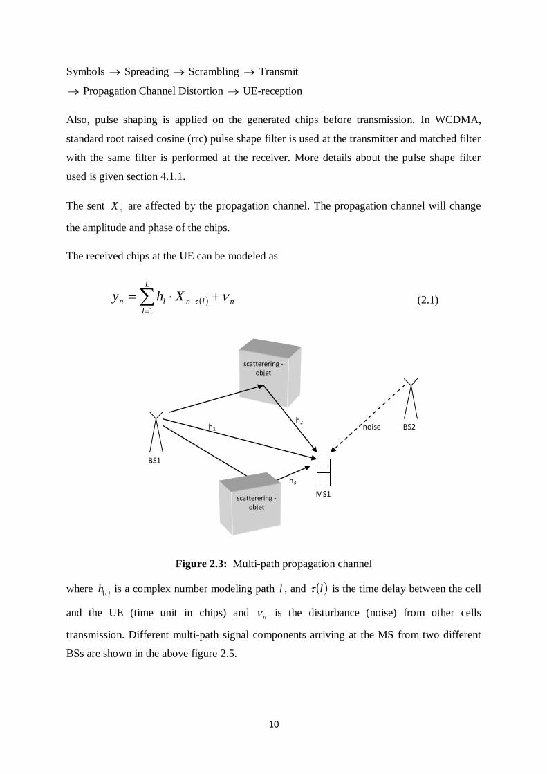
The received chips at the UE can be modeled as
L
l
nlnln Xhy1
(2.1)
Figure 2.3: Multi-path propagation channel
where lh is a complex number modeling path l , and l is the time delay between the cell
and the UE (time unit in chips) and n is the disturbance (noise) from other cells
transmission. Different multi-path signal components arriving at the MS from two different
BSs are shown in the above figure 2.5.
h3
noise h2
h1
MS1
BS1
BS2
scatterering - objet
scatterering - objet
11
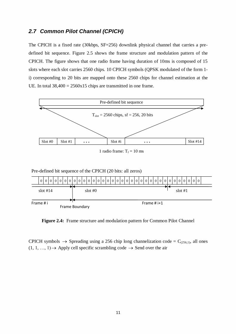
2.7 Common Pilot Channel (CPICH)
The CPICH is a fixed rate (30kbps, SF=256) downlink physical channel that carries a pre-
defined bit sequence. Figure 2.5 shows the frame structure and modulation pattern of the
CPICH. The figure shows that one radio frame having duration of 10ms is composed of 15
slots where each slot carries 2560 chips. 10 CPICH symbols (QPSK modulated of the form 1-
i) corresponding to 20 bits are mapped onto these 2560 chips for channel estimation at the
UE. In total 38,400 = 2560x15 chips are transmitted in one frame.
Figure 2.4: Frame structure and modulation pattern for Common Pilot Channel
CPICH symbols Spreading using a 256 chip long channelization code = C(256,1), all ones
(1, 1, …, 1) Apply cell specific scrambling code Send over the air
Slot #14
Pre-defined bit sequence of the CPICH (20 bits: all zeros)
Frame # i+1 Frame # i
Slot #0
Pre-defined bit sequence
Tslot = 2560 chips, sf = 256, 20 bits
Slot #1 . . . Slot #i . . .
1 radio frame: Tf = 10 ms
chips, 20 bits
0 0 0 0 0 0 0 0 0 0 0 0 0 0 0 0 0 0 0 0 0 0 0 0 0 0 0 0
0 0 0 0 0 0
slot #0 slot #14 slot #1
Frame Boundary
12
2.8 Example Using WCDMA
Assume an AWGN channel with the following impulse response
,0
,1lh ,
,4,3,2
1
l
l
Assume that 256 chips are received corresponding to one CPICH symbol. The chips received
at the UE can be expressed as
inn Xy
codestion channeliza orthogonal using cell same thefromsent usersor channelsother nO
BSsother from received chips ce,interferen cell-internq
The subscript „n‟ shows the chip index and superscript „i‟ is used for a channelization code.
Now if the received signal ny is correlated with the conjugate of inX and normalized by
2561 , we have the following expression
255
0
2
1
255
0 256
1.
256
1
n
i
n
n
i
nn XXy
CPICHthetoorthogonalcodes
tionchannelizausechannelsother0
255
0
.256
1
n
i
nn Xq
1.
256
1 255
0n
i
nn Xy
And the expected value of the power is then
2
2255
0
1.256
1
EXyE
n
i
nn
13
Now
Re21122 EE
Since inn Xq & are uncorrelated and 0 i
nn XEqE , this implies
2561.
256
111
2255
0
2
1
2
2
2
n
i
nn XEqEE
where 22
nqE and equals the average power of the inter-cell interference.
2.8.1 Propagation Channel Delay Time Estimation
We will use the CPICH again in our analysis now to detect the time location of the
propagation channel paths. The signal received at the UE is given by
L
l
lnlnln OcellthefromchannelsotherXhy1
.
+ Inter-cell Interference nq
(2.3)
where nX is the chip sequence containing the CPICH symbols, channelization code, and
scrambling code. And L represent the number of multi-paths arriving at the MS from Node
B.
For different time/chips shifted version of nX , lets define the correlation of ny with mnX
as follows:
mnn
L
l n
mnlnlnl
n
mnnm XqXOXhXyZ1
255
0
255
0
.
The expectation value of mZ is
Llsomeforlm
LlsomeforlmhZE
l
m,,1,0
,,1,256
(2.4)
The result follows from the fact that nq &
mnX are uncorrelated due to different scrambling
codes, nO &
mnX are orthogonal if ,0m and uncorrelated if 0m due to scrambling code
14
properties. Similarly nX &
mnX are uncorrelated if 0m from the scrambling code
properties.
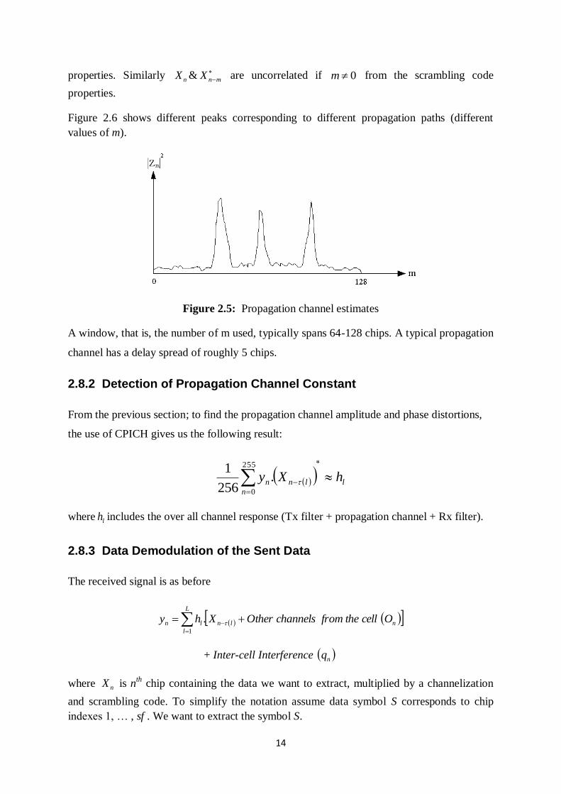
Figure 2.6 shows different peaks corresponding to different propagation paths (different
values of m).
Figure 2.5: Propagation channel estimates
A window, that is, the number of m used, typically spans 64-128 chips. A typical propagation
channel has a delay spread of roughly 5 chips.
2.8.2 Detection of Propagation Channel Constant
From the previous section; to find the propagation channel amplitude and phase distortions,
the use of CPICH gives us the following result:
l
n
lnn hXy
255
0
.256
1
where lh includes the over all channel response (Tx filter + propagation channel + Rx filter).
2.8.3 Data Demodulation of the Sent Data
The received signal is as before
L
l
nlnln OcellthefromchannelsOtherXhy1
.
+ Inter-cell Interference nq
where nX is nth
chip containing the data we want to extract, multiplied by a channelization
and scrambling code. To simplify the notation assume data symbol S corresponds to chip
indexes 1, … , sf . We want to extract the symbol S.
15
Figure 2.6: Data Demodulation Using RAKE
2.8.3.1 RAKE
The despreading is done in the RAKE, that is, correlate ny with lnX
~, where nX
~ is the
chip sequence formed by the channelization code and scrambling code of the desired user or
symbol. Rake outputs are obtained for l paths or braches as described in the following
equation and also shown in figure 2.7.
ShXysf
r l
sf
n
lnnl
1
0
~.
1
by using the below mentioned results
nm
nmSXX
sf
sf
n
lmln,0
,.
~11
0
1
0
0.~1 sf
n
ln channelsOtherXsf
1
0
0.~1
sf
n
ln ceInterferenIntercellXsf
A simple block diagram showing the operations required to extract the sent symbol S is
shown in figure 2.8.
y
Decoded Symbols
RAKE Channel
Estimator
Combiner
Decoder
Spread data received
from a number of cells
16
2.8.3.2 Channel Estimation
Using the CPICH we can estimate lh , since the symbol S is then known. In a slot, we have
10 CPICH symbols and consequently we have 10 channel samples per slot, call them
10,,1,, ihsamp
il
To calculate a channel estimate, use the average of the samples over a slot, that is,
10
1
,10
1
i
samp
il
est
l hh
Or the channel samples can be filtered by using the following equation:
10,,1,1 1,,, ihhh est
ilh
samp
ilh
est
il
2.8.3.3 Interference Estimation
An estimate of the inter-cell interference is found from
10
1
2
, ,,1,9
1
i
est
l
samp
ill LlhhI
To be precise, the expectation value of lI also contains inter-symbol interference from the
cell we are trying to demodulate. That is, the different paths carry own copy of the sent signal
and since they are not time-aligned, they will interfere with each other.
2.8.3.4 Signal-to-Interference Ratio (SIR)
SIR is defined as:
L
l l
est
l
I
hSIR
1
2
and is computed once per slot. It is a quality measure of the propagation channel. The higher
the ratio the lesser the errors will be made when determining the sent data.
17
2.8.3.5 Combiner
The sent symbol S is recovered by multiplying the RAKE output with the conjugate of the
channel estimates, that is,
S
I
hh
I
rh L
l l
l
est
lL
l l
l
est
l ...
11
A real positive value is obtained if est
lh is well estimated. We divide by lI to favor paths
experiencing low interference. Figure 2.8 shows the operations of a simple RAKE receiver
with combiner output.
Figure 2.7: RAKE Receiver Block Diagram
Output
Data Bits
yn
Multiple RAKE Fingers to
Receive the Input Signal
g3
gL
g2
g1
τ1
τ2
τ3
τL
...
Symbol
Mapper
Received Samples
Descrambling/Despreading
Channel Estimation / Equalizer
Weights and Maximum Ratio
Combining (MRC)
...
...
18
Chapter 3
3 Equalizer Model
3.1 Communication System Diagram
Figure 3.1: Communication System Block Diagram
3.2 RAKE (Time domain)
A simplified RAKE receiver block diagram is shown in figure 2.7. The filter (equalizer)
weights shown in that figure can be determined in several ways for time domain equalization.
Here, we consider the following two methods
1) Non-parametric MMSE-based Equalization
2) ML-based Equalization (Nonparametric GRAKE)
Radio
Channel Symbol
Stream
Chip
Stream
RRC filter
(pulse-shaping) D/A
y
Radio
Channel
Radio A/D RRC filter
(pulse-shaping)
19
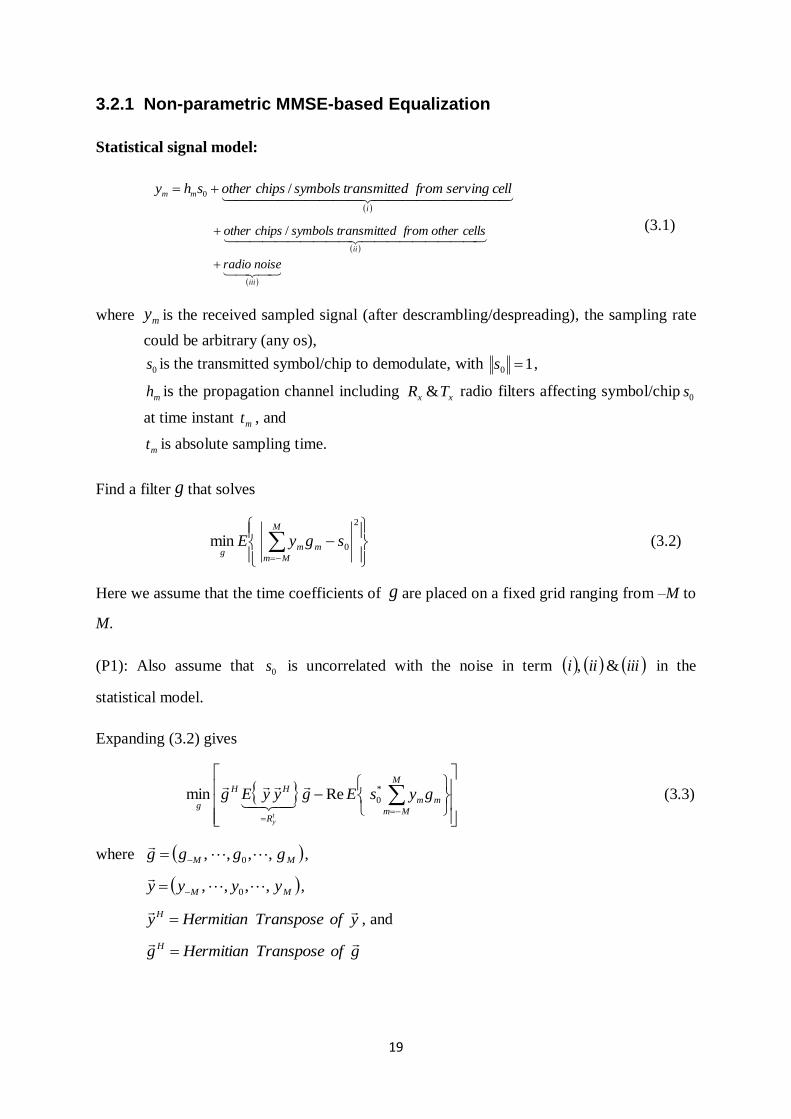
3.2.1 Non-parametric MMSE-based Equalization
Statistical signal model:
i
mm cellservingfromdtransmittesymbolschipsothershy /0
ii
cellsotherfromdtransmittesymbolschipsother / (3.1)
iii
noiseradio
where my is the received sampled signal (after descrambling/despreading), the sampling rate
could be arbitrary (any os),
0s is the transmitted symbol/chip to demodulate, with 10 s ,
mh is the propagation channel including xx TR & radio filters affecting symbol/chip 0s
at time instant mt , and
mt is absolute sampling time.
Find a filter g that solves
2
0minM
Mm
mmg
sgyE (3.2)
Here we assume that the time coefficients of g are placed on a fixed grid ranging from –M to
M.
(P1): Also assume that 0s is uncorrelated with the noise in term iiiiii &, in the
statistical model.
Expanding (3.2) gives
M
Mm
mm
R
HH
ggysEgyyEg
ty
*
0Remin
(3.3)
where MM gggg ,,,, 0
,
MM yyyy ,,,, 0
,
yofTransposeHermitianyH , and
gofTransposeHermitiang H
20
Since 12
0 s , the assumptions in (P1) gives us
M
Mm
mm
M
Mm
mm ghgysE ReRe *
0 12
0
*
00 sss
Thus (3.3) can be written as,
M
Mm
mm
R
HH
gghgyyEg
ty
Remin
(3.4)
Taking the derivate of (3.4) w.r.t g and solving for zero gives, see Appendix B
*1hRg t
y
(3.5)
where MM hhhh ,,,, 0
and by omitting the scalar multiplier in the (3.5).
Here yR can be computed by filtering the received samples as
lknn
old
yy yyklRklR *)1(,, (3.6)
where the filtering parameter depends on the Doppler spread.
3.2.2 ML-based Equalization (Non-parametric G-RAKE)
Referring back to (3.1)
mmm nshy 0
where mn is modeling the unwanted part of the received signal, that is, the noise.
Assume we have Mm ,,1 sampled my ; collect them into a vector Myyy ,,1 . Let‟s
then try to fit the vector y
to a multi-dimensional probability distribution. A first choice is
the Gaussian probability distribution, since it is simple to manipulate and contains few
parameters to estimate.
Assuming the probability distribution for y
to be Gaussian, we have the following pdf
0
10 shyRshy n
H
e
(3.7)
where MM hhhh ,,,, 0
21
and nR is the covariance matrix of the noise defined as
*
2121mmmmn nnER
Maximizing (3.7) with respect to0s , that is, take the derivative of (3.7) with respect to
0s and
solve the result for0s . Then,
0s is given by
yhRst
t
n
*1
0
, (3.8)
by omitting a scalar factor 11
hRh n
H
.
Comparing with (3.5) shows that the filter g here is given by *1hR t
n
and in (3.5) is given
by *1hRt
y
.
Assuming the noise mn is uncorrelated with 0shm , we have
H
y nshnshER
00
n
HHH RhhnnEhhs
1
2
0 (3.9)
In practice, it is difficult to estimate nR without knowing the sent symbol 0s . If, however, we
have a pilot channel, modeled as
mmm nphy ~0 (3.10)
The noise mn~ is of the same nature as mn (which is most often the case); we can now estimate
nR based on the pilot channel, that is,
**
0
*
0 221121
est
mm
est
mmmmn hpyhpyR
Here est
mh is an averaged or filtered version of the samples *
0pym , for example,
est
oldmhmh
est
m hpyh ,
*
0 1 (3.11)
Also less variations in nR can be had by applying filtering as below
filt
oldnRnR
filt
n RRRnn ,1 (3.12)
22
3.2.3 SIR
For both MMSE and ML methods, the demodulated symbol/chip is given by the following
equation
yhRst
*1
0
where the matrix R is given by t
yR if the filter g is computed using the MMSE method and
t
nR if the ML method is used.
Given the model in (3.1)
100 snshy
by multiplying the above equation with the filter g , we get
nhRshhRyhRttt
*1
0
*1*1 (3.13)
The signal-to-interfernce ratio is defined as
**1**1
2*1
2*1
2
0
*1
hRnnhRE
hhR
nhRE
shhRSIR
tt
t
t
t
**1*
2*1
**1**1
2*1
hRRRh
hhR
hRnnEhR
hhR
n
tt
t
tt
t
For the ML method matrixidentityIRR n
t
hhR
hhR
hhR
hRh
hhRSIR
t
t
t
t
t
*1
**1
2*1
**1*
2*1
For the MMSE method no such reduction is possible.
In practice, the numerator in SIR is replaced by 2
*1 yhRt
. The expectation value of this is
2
*12
*1 nhREhhRtt
1 SIRSIRpractical
23
Also
2*1 nhRE
t in the denominator of SIR is computed by averaging the square of
sample
tt
nphhRyhR
*1*1 (3.14)
Where p are known pilot symbols. From (3.13) we get that the above difference equals
nhRt
*1 . Let isamplen , be a number of collected samples, then an estimate of
2*1 nhRE
t is given by
Samples
i
isamplesnSamples
#
1
2
,#
1
If the ML-method is used and we are confident that the used R approximates well t
nR , then
the simplified expression hhRt
*1 can be used for SIR .
3.3 FFT (Frequency domain)
3.3.1 System Model
Time domain signal ty at the receiver is modeled as below
,1 1
P
p m
L
l
lchip
p
mp
prop
l noisemtcahty (3.15)
where p enumerates the physical channels;
m enumerates the chips;
l enumerates the propagation paths; prop
lh is a complex valued propagation channel;
pa is the signal amplitude;
p
mc is the chip at index m for pth
channel (composed of channelization code,
scrambling code, and the sent symbol);
is the pulse shaping filter; and
l is the propagation path delay for signal path l.
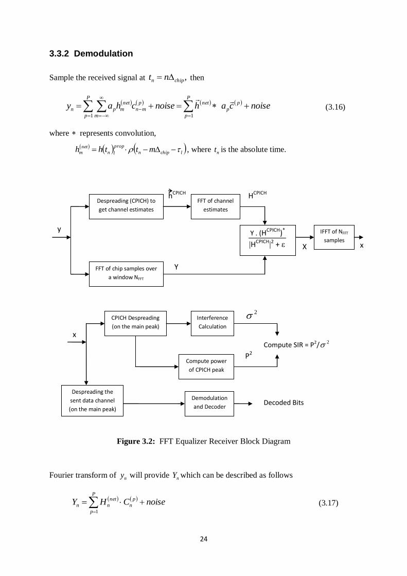
Figure 3.2 shows the different blocks used in the FFT equalizer receiver. Functioning detail
about respective blocks is provided in the coming sections.
24
3.3.2 Demodulation
Sample the received signal at ,chipn nt then
noisecahnoisechay
P
p
p
p
netP
p m
p
mn
net
mpn
11
(3.16)
where represents convolution,
lchipn
prop
ln
net
m mtthh , where nt is the absolute time.
Figure 3.2: FFT Equalizer Receiver Block Diagram
Fourier transform of ny will provide nY which can be described as follows
P
p
p
n
net
nn noiseCHY1
(3.17)
X x
Demodulation
and Decoder
P2
2
Y
HCPICH hCPICH
y
Despreading (CPICH) to
get channel estimates
FFT of channel
estimates
FFT of chip samples over
a window NFFT
Y . (HCPICH)*
x
IFFT of NFFT
samples
CPICH Despreading
(on the main peak)
Interference
Calculation
Compute power
of CPICH peak
Compute SIR = P2/ 2
Despreading the
sent data channel
(on the main peak) Decoded Bits
|HCPICH|2 + ε
25
where net
nH is the Fourier transform of neth
and
p
nC is the Fourier transform of p
pca
For the MMSE based equalizer, the influence of netH is removed to obtain nX as shown
below in equation (3.18)
2
2
*
net
n
net
nnn
H
HYX (3.18)
where 2 is the estimate of noise variance and *net
nH is the complex conjugate of net
nH .
Eq. (3.18) refers to the MMSE based equalizer, which is explained next. Now referring back
to (3.1): for a signal model
noiseshy
where „s‟ is the transmit symbol/chip. Find a filter „w‟, such that the following expression is
minimized:
2min swyE
w
2min noisewswshE
w
swshswshwswshw
**22222
min
whwshw
Re2min222
By solving for „w‟ gives
22
*
h
hw
22
*
h
hywys
In the simulations, we will use (3.19) for the required channel cancellation operation as
follows:
26
2
*
net
n
net
nnn
H
HYX (3.19)
where „ε‟ can be called a regularization term which needs to be tuned depending on the
propagation channel profile and on the signal-to-noise ratio value at the receiver.
3.3.3 Approximations to investigate
The following approximations will be investigated:
1- The Fourier transform needs to be finite, that is, a finite number of samples can only
be handled at a time. Investigate optimal (smallest) number of samples for different
channels.
2- The amount of filtering needs to be tuned for filtered channel estimate net
nfilteredh , as
shown in (3.23).
3- The amount of filtering needs to be tuned for interference estimation 2
,kfiltered as
shown in (3.22).
3.3.4 Interference Calculation
After applying IFFT on nX to come back to time domain, we get „x‟ which can be modeled
as
P
p
p
npn noisecax1
(3.19)
Assume 1p for the CPICH. Despreading of „x‟ with the scrambling code and then the
channelization code of 1p will give
k
kn
CPICH
ksamplenn xcx256
25611
,
*1.256
1 (3.20)
where „k‟ refers to the CPICH symbols received by despreading of the chip samples. Ten
CPICH symbols are received from one WCDMA slot.
The received CPICH symbols are filtered as below:
CPICH
ksampleh
CPICH
kfilteredh
CPICH
kfiltered xxx ,1,, .1
The interference is further estimated as,
,2
,
2
,, ksample
CPICH
ksample
CPICH
kfiltered xx (3.21)
27
To get the final 2 , filter 2
,ksample
2
,
2
kfiltered , where
2
,
2
1,
2
, 1 ksamplekfilteredkfiltered (3.22)
3.3.5 Power Calculation
To calculate the received signal power, let 2
,
CPICH
kfilteredest xp . Filter estp as in (3.22) and call it
P .
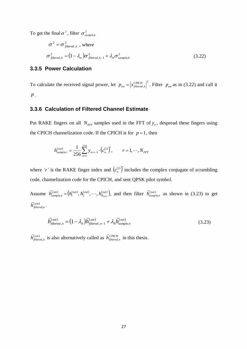
3.3.6 Calculation of Filtered Channel Estimate
Put RAKE fingers on all FFTN samples used in the FFT of ny , despread these fingers using
the CPICH channelization code. If the CPICH is for 1p , then
FFT
n
nrn
net
rsample Nrcyh ,,1,256
1 256
1
*1
1,
where „r‟ is the RAKE finger index and *1
nc includes the complex conjugate of scrambling
code, channelization code for the CPICH, and sent QPSK pilot symbol.
Assume net
N
netnetnet
nsample FFThhhh ,,, 21,
, and then filter
net
nsampleh ,
as shown in (3.23) to get
net
nfilteredh ,
.
net
nsampleh
net
nfilteredh
net
nfiltered hhh ,1,, 1
(3.23)
net
nfilteredh ,
is also alternatively called as
CPICH
nfilteredh ,
in this thesis.
28
Chapter 4
4 Implementation and Results
4.1 Simulation Setup
Both the methods described in sections 3.2 and 3.3 for channel equalization are implemented
in IT++. Standard library features of IT++ are used to construct different blocks of the
transmitter, receiver, and the propagation channel. Simulation parameters used for the
WCDMA transmit signal are given below.
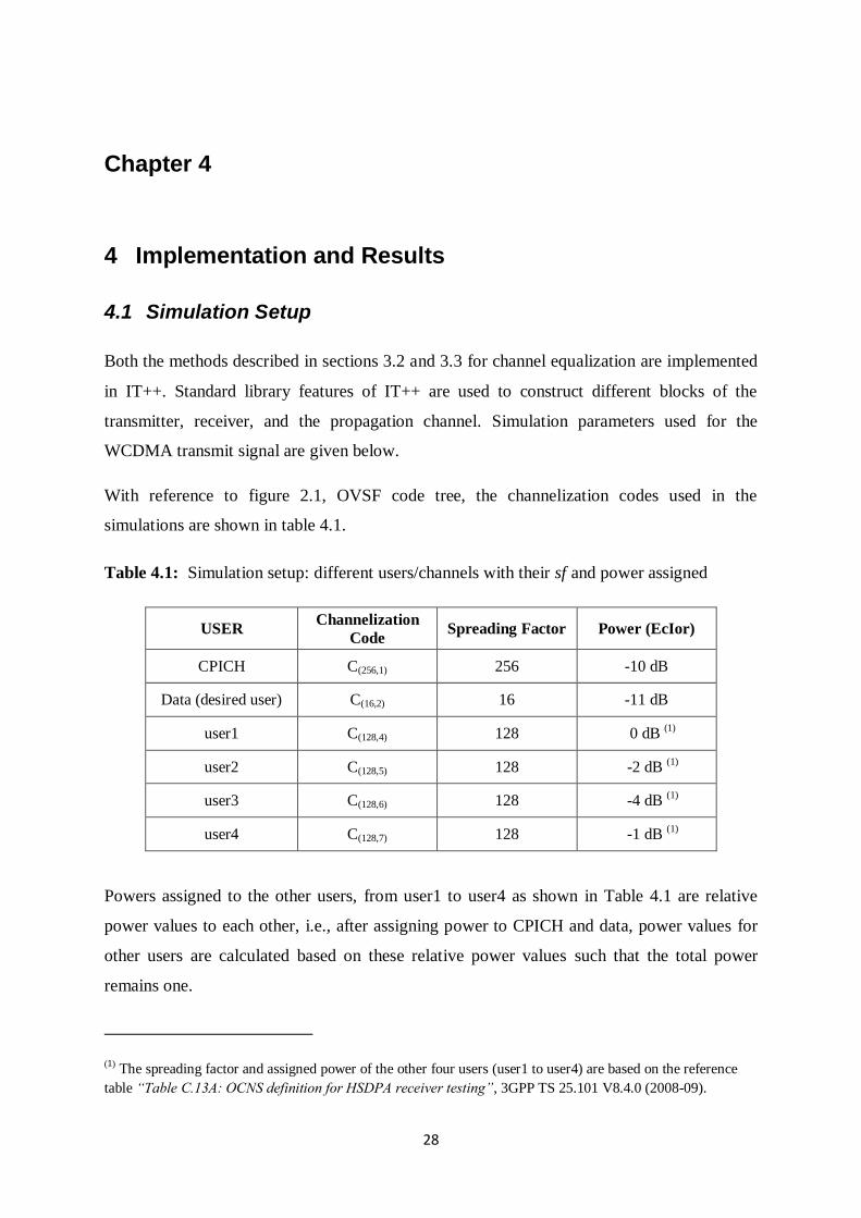
With reference to figure 2.1, OVSF code tree, the channelization codes used in the
simulations are shown in table 4.1.
Table 4.1: Simulation setup: different users/channels with their sf and power assigned
USER Channelization
Code Spreading Factor Power (EcIor)
CPICH C(256,1) 256 -10 dB
Data (desired user) C(16,2) 16 -11 dB
user1 C(128,4) 128
0 dB (1)
user2 C(128,5) 128 -2 dB (1)
user3 C(128,6) 128 -4 dB (1)
user4 C(128,7) 128 -1 dB (1)
Powers assigned to the other users, from user1 to user4 as shown in Table 4.1 are relative
power values to each other, i.e., after assigning power to CPICH and data, power values for
other users are calculated based on these relative power values such that the total power
remains one.
(1) The spreading factor and assigned power of the other four users (user1 to user4) are based on the reference
table “Table C.13A: OCNS definition for HSDPA receiver testing”, 3GPP TS 25.101 V8.4.0 (2008-09).
29
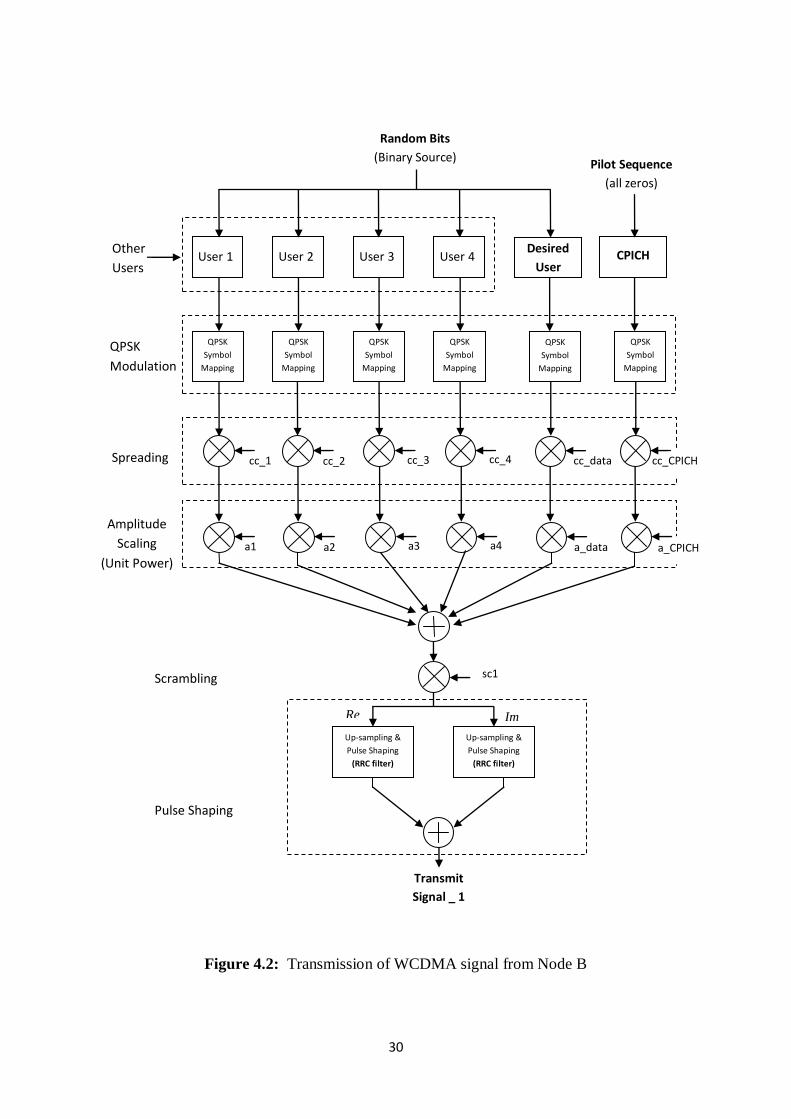
4.1.1 Transmit Signal from Node B
Figure 4.2 shows the simulation flow to construct a WCDMA transmit signal at Node B
which carries information for all the users/channels mentioned in table 4.1. The information
for different users/channels is spread with the use of their respective channelization codes.
Scrambling code used at the BS (Node B) is marked as „sc1‟ which is uniquely assigned to
the BS. And any other scrambling code may be employed for transmission from other BS.
CPICH uses all zero bits, whereas, random bits are generated for other users as well as for the
desired data user. QPSK is used as the modulation scheme for both for the data users and for
CPICH.
Half slot processing is employed, i.e., 1280 chips are processed at one time. Same
channelization codes are used each time to spread the different data symbols, while
scrambling code is repeated after every 38400 chips. Spreading factor of 16 for the data user
implies that 1280/16 = 80 QPSK data symbols can be transmitted through each half slot.
Similarly, 5 CPICH symbols and 10 other data user‟s symbols are transmitted at one time.
Before scrambling, each user/channel signal is multiplied with its respective amplitude. The
signal amplitudes are calculated based on the signal power values mentioned in table 4.1 and
the overall signal energy is kept as unity.
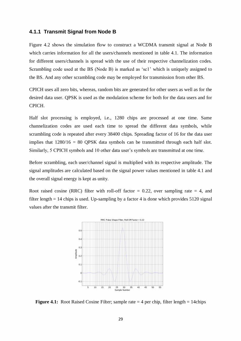
Root raised cosine (RRC) filter with roll-off factor = 0.22, over sampling rate = 4, and
filter length = 14 chips is used. Up-sampling by a factor 4 is done which provides 5120 signal
values after the transmit filter.
Figure 4.1: Root Raised Cosine Filter; sample rate = 4 per chip, filter length = 14chips
5 10 15 20 25 30 35 40 45 50 55
-0.1
0
0.1
0.2
0.3
0.4
0.5
Sample Number
Am
plitu
de
RRC Pulse Shape Filter, Roll Off Factor = 0.22
30
Figure 4.2: Transmission of WCDMA signal from Node B
Re Im
a_CPICH
cc_CPICH
a_data
sc1
cc_1 cc_2 cc_3 cc_4 cc_data
Random Bits
(Binary Source)
QPSK
Symbol
Mapping
User 1 User 2 User 3 User 4 CPICH
QPSK
Symbol
Mapping
QPSK
Symbol
Mapping
QPSK
Symbol
Mapping
QPSK
Symbol
Mapping
a1 a2 a3 a4
Transmit
Signal _ 1
Up-sampling &
Pulse Shaping
(RRC filter)
Up-sampling &
Pulse Shaping
(RRC filter)
Other
Users
QPSK
Modulation
Spreading
Desired
User
QPSK
Symbol
Mapping
Amplitude
Scaling
(Unit Power)
Scrambling
Pilot Sequence
(all zeros)
Pulse Shaping
31
4.1.2 Propagation Channel
The propagation channel model used in the simulations is a two path non-fading (static)
channel. The power is divided equally between the two paths. Different values of delay
spread are simulated; and the results are shown in section 4.4 and onwards. Single path
channel model and ITU-Pedestrian B with speed 3km/hr (PB3) which is a slow fading
channel; are also used in the simulations.
4.1.3 Signal Reception at UE
The up-sampled signal values are received at UE through a propagation channel. The receiver
functions are shown in figure 4.3. WCDMA signal from the desired BS as well as from
another nearby BS, which is using a different scrambling code, is received at MS through a
wireless channel.
Additive White Gaussian Noise (AWGN) is added to the received signal. Equalizer
performances on different values of noise variance are tested by various simulations. Also
without AWGN, equalizer performance is observed. Frequency errors are generated at the UE
due to any phase offset or synchronization loss between the clocks of the BS and MS.
Receiver performance with and without frequency errors are then tested. Analog-to-Digital
converter (A/D) is used to digitize the received signal before filtering operation. Equalizers
performance with different (A/D) converters are simulated and shown in the results section
4.4.
Received signal is finally fed to the receiver filter which is also a root raised cosine (RRC)
filter matched to the transmit filter. Matched filter output is then used for both equalizers.
32
Figure 4.3: Received Signal at UE via Matched Filtering
yrec
Transmit
Signal _ 1
Propagation
channel
AWGN
ej2.pi.f.Ts Frequency Errors at UE
(f in Hz, Ts – current sample time)
A/D
FFT Equalizer
Receiver
GRAKE Equalizer
Receiver
Transmit
Signal _ 2
WCDMA Signal from
another BS (Node B),
scaled appropriately
Re Im
Matched Filtering
(RRC filter)
Matched Filtering
(RRC filter)
Matched
Filtering
33
4.2 GRAKE Equalizer Receiver
4.2.1 Channel Estimation
Received signal values after the receiver filter are used to detect the channel response to the
transmit signal. In figure 4.4, different blocks are shown which are used in the simulator to
detect the channel response on different signals received via multiple rake fingers.
Figure 4.4: Non-Parametric G-RAKE Receiver Channel Estimation
τ = ¾ chip delay;
(2m+1+ds) = # of fingers;
ds = (delay_spread / τ)
sampleh
filteredh
hm+ds hm+ds-1
RAKE Fingers
h0
... sc1
...
sc1
h-m+1 h-m
cc_CPICH cc_CPICH
...
Averaging
Filter
∑ ∑
Descrambling
Despreading
Divide by
Known Pilot
(0.707+0.707i)
Divide by
Known Pilot
(0.707+0.707i)
...
...
(-m).τ (-m+1).τ ...
...
...
cc_CPICH
sc1
∑
Divide by
Known Pilot
(0.707+0.707i)
(m+ds-1).τ
cc_CPICH
sc1
∑
Divide by
Known Pilot
(0.707+0.707i)
0.τ
Channel
Estimation
Divide by
Known Pilot
(0.707+0.707i)
cc_CPICH
sc1
∑
(m+ds).τ
yrec
DS DS DS DS DS
Downsampling
Chip Offset
(0, ¼, ½ ) ... ...
34
GRAKE uses (2m+1+ds) fingers which are separated by a fixed time delay between any two
rake fingers, i.e., „τ‟ equals to ¾ chip delay. Different delayed versions of the WCDMA
signal are received via these fingers. Depending on the xx TR & filter length, the parameter
„m‟ is selected as 20 = 15/τ, to collect all the energy stored in the filter taps; while „ds‟ is the
delay spread (time difference between LOS signal path and the last significant signal energy
path) divided by the finger spacing (τ). In this thesis „ds‟ or path delay will be referring to the
delay (in # of chips) between two equal energy signal paths. RAKE finger placed at (0.τ)
implies zero delay is introduced and direct despreading is used. For single path test cases,
nine fingers with fifth finger at the zero delay position are used in the test simulations (nine
fingers are considered to be optimum number in this case).
Downsampling is performed on each rake finger as there is upsampling done at the
transmitter side before transmission. Different offset positions are used as shown in the figure
4.3 to simulate the GRAKE equalizer performance for the time offset received data.
Descrambling and despreading operations are implemented to recover the original sent
symbols. Desired scrambling code „sc1‟ for the BS scrambling and „cc_CPICH‟ is used for
the CPICH channel. Since the CPICH symbols are known at the UE, dividing with the known
symbols return the channels estimate values on the respective rake fingers. Since five CPICH
symbols are received in one half slot, averaging filter is implemented to filter the sampled
channel estimates. The filtered channel estimate is then used for the estimation of noise
covariance matrix and further the G-RAKE equalizer filter weights.
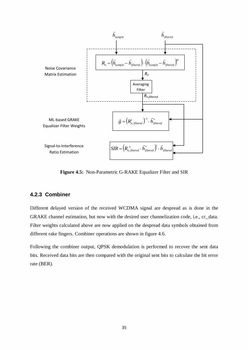
4.2.2 Equalizer Filter and SIR
Based on the sampled channel values and the filtered estimate, noise covariance matrix is
calculated as shown in figure 4.5. Further, filtered channel estimate and filtered noise
covariance matrix are used to determine the equalizer filter weights and an estimate of
Signal-to-Interference ratio. Noise covariance matrix inversion is implemented by using
standard built-in functions available in IT++ for calculating matrix inverse.
35
Figure 4.5: Non-Parametric G-RAKE Equalizer Filter and SIR
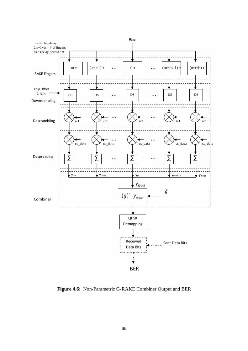
4.2.3 Combiner
Different delayed version of the received WCDMA signal are despread as is done in the
GRAKE channel estimation, but now with the desired user channelization code, i.e., cc_data.
Filter weights calculated above are now applied on the despread data symbols obtained from
different rake fingers. Combiner operations are shown in figure 4.6.
Following the combiner output, QPSK demodulation is performed to recover the sent data
bits. Received data bits are then compared with the original sent bits to calculate the bit error
rate (BER).
Rn
filteredh
sampleh
Rn,filtered
ML-based GRAKE
Equalizer Filter Weights *1
, filtered
t
filteredn hRg
Hfilteredsamplefilteredsamplen hhhhR
Noise Covariance
Matrix Estimation
Averaging
Filter
filtered
t
filteredfilteredn hhRSIR *1
, Signal-to-Interference
Ratio Estimation
36
Figure 4.6: Non-Parametric G-RAKE Combiner Output and BER
ym+ds ym+ds-1 y0 y-m+1 y-m
τ = ¾ chip delay;
2m+1+ds = # of fingers;
ds = (delay_spread / τ)
g
RAKEy
RAKE Fingers
... sc1 sc1
... ... cc_data cc_data
yrec
...
∑ ∑
Descrambling
Despreading ...
-m.τ (-m+1).τ ...
...
...
cc_data
sc1
∑
(m+ds-1).τ
cc_data
sc1
∑
0.τ
cc_data
sc1
∑
(m+ds).τ
RAKE
tyg
Combiner
BER
QPSK
Demapping
Received
Data Bits Sent Data Bits
DS DS DS DS DS
Downsampling
Chip Offset
(0, ¼, ½ ) ... ...
37
4.3 FFT Equalizer Receiver
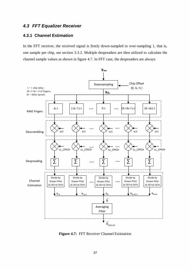
4.3.1 Channel Estimation
In the FFT receiver, the received signal is firstly down-sampled to over-sampling 1, that is,
one sample per chip, see section 3.3.2. Multiple despreaders are then utilized to calculate the
channel sample values as shown in figure 4.7. In FFT case, the despreaders are always
Figure 4.7: FFT Receiver Channel Estimation
yds
filteredh
τ = 1 chip delay;
2k+1+ds = # of fingers;
ds = delay spread.
h0 h-k h-k+1 hk+ds hk+ds-1
...
...
...
...
cc_CPICH
h
cc_CPICH ...
cc_CPICH cc_CPICH
Chip Offset
(0, ¼, ½ )
yrec
Downsampling
...
Averaging
Filter
sc1 sc1 sc1
∑ ∑ ∑
Descrambling
Despreading
Divide by
Known Pilot
(0.707+0.707i)
Divide by
Known Pilot
(0.707+0.707i)
Divide by
Known Pilot
(0.707+0.707i)
...
... Channel
Estimation
sc1
∑
Divide by
Known Pilot
(0.707+0.707i)
cc_CPICH
sc1
∑
Divide by
Known Pilot
(0.707+0.707i)
-k.τ (-k+1).τ ... ... (k+ds-1).τ 0.τ (k+ds).τ RAKE Fingers
38
separated by one chip delay while descrambling and despreading operations to get the
channel sample values are the same as performed in the GRAKE channel estimation.
Based on the xx TR & radio filters which are used as standard root raised cosine filters with
filter length equals to 14 chips as shown in figure 4.1, the parameter „k‟, i.e., the number of
despreaders used in the left of the main peak is chosen as 15; while the number of
despreaders towards the right of the main peak are chosen as (15+ds). For single path test
cases, ds = 0 is used. In that case, 31 despreaders are used to calculate the channel estimate,
15 despreaders on both sides of the zero delay despreader.
4.3.2 Equalizer
Equalization operation is performed in the frequency domain. Both the channel estimates
values and received down sampled signal is converted to frequency domain by taking Fast
Fourier Transform (FFT). FFT function is used as a standard IT++ library function. Figure
4.8 shows the method used in the FFT equalization operation.
The channel equalization is performed on each half slot received. The channel estimate vector
used in the FFT equalizer has 1280 chips with the channel estimate values obtained by
(2k+1+ds) despreaders in the centre and rest of the values as zeros.
A parameter tuning block as shown in figure 4.8 is also used in the FFT equalizer method for
parameters tuning. An output of the intelligent block, „ε‟ is required in the channel
equalization operation. The value of „ε‟ depends on the values of IorIoc, delay spread, and
the size of the A/D used. Optimal values of „ε‟ are found for different values of IorIoc and
delay spread. The optimal values of „ε‟ needs to be scaled with the same A/D constant (K)
used for multiplying the signal before quantization. Different A/D sizes and their respective
A/D constant (K) values are used in the simulations.
As the equalization is performed in the frequency domain, so an inverse Fourier Transform
(IFFT) is used to convert the equalized signal back to the time domain signal. In the figure, it
is also shown that the number of chips that can be used further for despreading and symbol
detection is decided by the parameter tuning block‟s output „M‟. The value of M depends on
the delay spread and target BER. For small delay spread channels, more chips are equalized
as compared to large delay spread channels. More details about the number of output chip
samples are given in section 4.4.6.1.
39
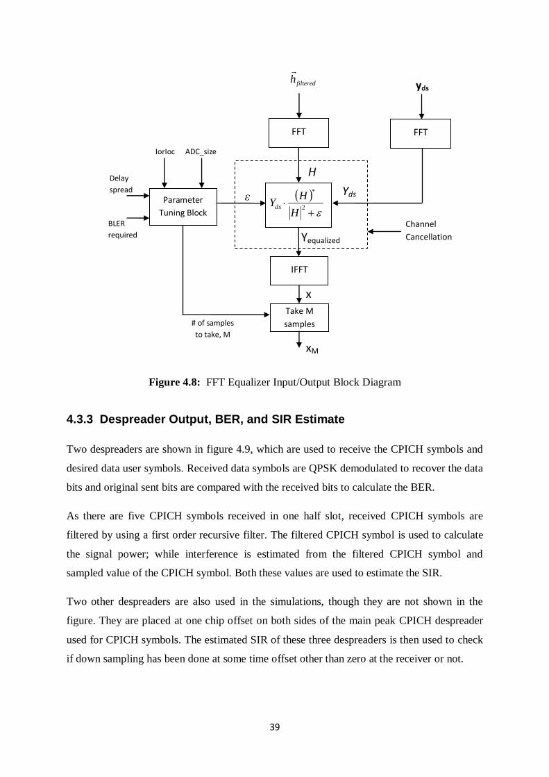
Figure 4.8: FFT Equalizer Input/Output Block Diagram
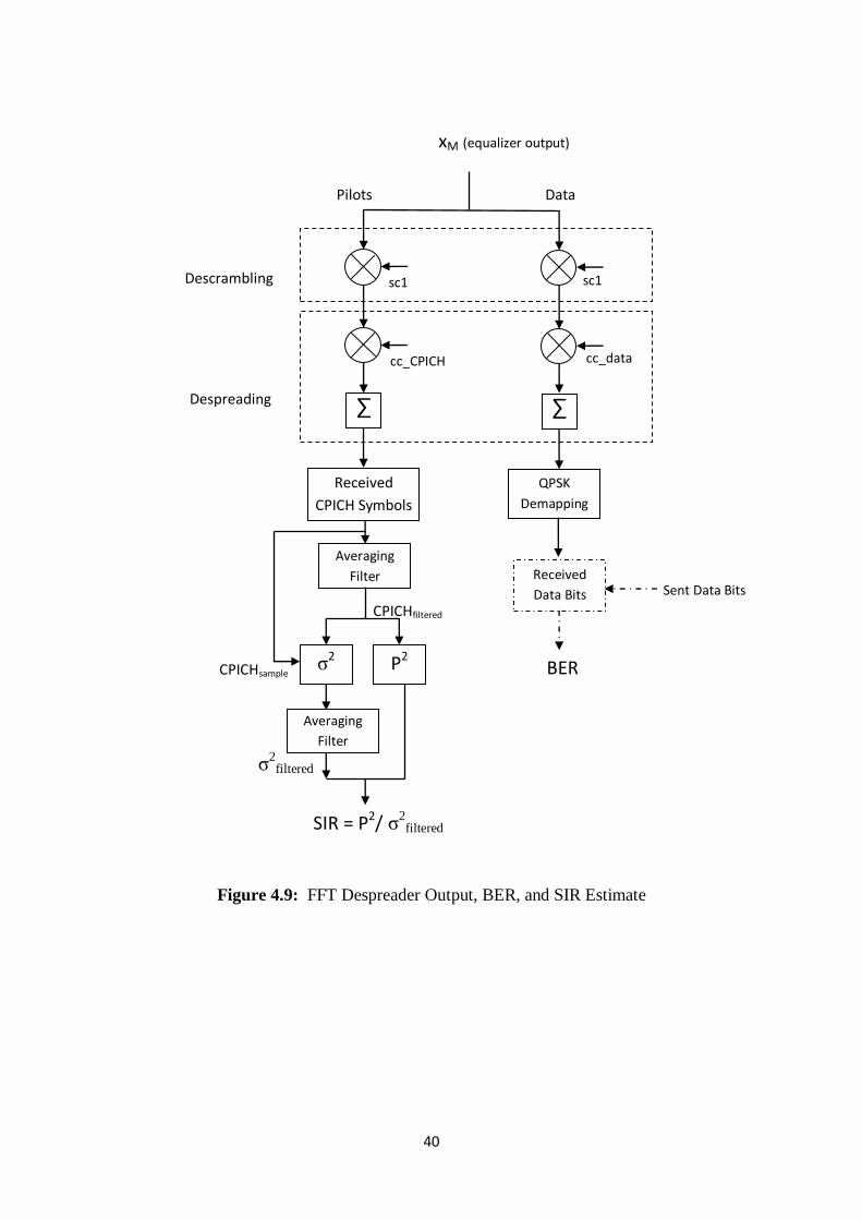
4.3.3 Despreader Output, BER, and SIR Estimate
Two despreaders are shown in figure 4.9, which are used to receive the CPICH symbols and
desired data user symbols. Received data symbols are QPSK demodulated to recover the data
bits and original sent bits are compared with the received bits to calculate the BER.
As there are five CPICH symbols received in one half slot, received CPICH symbols are
filtered by using a first order recursive filter. The filtered CPICH symbol is used to calculate
the signal power; while interference is estimated from the filtered CPICH symbol and
sampled value of the CPICH symbol. Both these values are used to estimate the SIR.
Two other despreaders are also used in the simulations, though they are not shown in the
figure. They are placed at one chip offset on both sides of the main peak CPICH despreader
used for CPICH symbols. The estimated SIR of these three despreaders is then used to check
if down sampling has been done at some time offset other than zero at the receiver or not.
x
xM
# of samples
to take, M
Yequalized
H
BLER
required
Delay
spread ε Yds
FFT
Parameter
Tuning Block
IorIoc ADC_size
Channel
Cancellation
yds
2
*
H
HYds
FFT
filteredh
IFFT
Take M
samples
40
Figure 4.9: FFT Despreader Output, BER, and SIR Estimate
Data Pilots
σ2filtered
CPICHsample BER
CPICHfiltered
P2
xM (equalizer output)
sc1 sc1
cc_data
∑
cc_CPICH
∑
QPSK
Demapping
Received
Data Bits Sent Data Bits
Received
CPICH Symbols
Averaging
Filter
Averaging
Filter
σ2
SIR = P2/ σ2filtered
Descrambling
Despreading
Averaging
Filter
Averaging
Filter
41
4.4 Results and Discussion
4.4.1 Parameters Optimization
4.4.1.1 GRAKE Parameters Optimization
Two averaging filters are implemented in the G-RAKE method. The averaging filter which is
used to filter the channel estimate results uses h ; and the second filter which is filtering the
noise covariance matrix uses nR as the filtering parameters as shown in (3.11) and (3.12)
respectively.
Simulations are performed for different channels (single path and two path non-fading or
static channels) and using different IorIoc values. For single path channel, nine fingers are
used to receive the WCDMA signal. And for two path channel, number of fingers used to
receive the WCDMA signal is calculated as (2m+1+ds), as discussed in section 4.2. Delay
spread „ds‟ = 5 chip is used for two path channel simulations.
Firstly, for an arbitrary value of h equals to 1/200 for our case, multiple simulations are
performed for IorIoc values starting from -4 dB and going up till 28 dB. For each IorIoc
value, a range of values fornR from 1/25 to 1/500 are simulated. From the simulation results,
BER performance of the data user is observed. Based on these results, optimum (largest)
value for nR is selected to be 1/200, for all the IorIoc values as well as for the two main test
cases, i.e., single path and two path channel with „ds‟ = 5 chip. A large value of nR is used to
give more weightage to the noise samples received in the current WCDMA slot.
Secondly, using the optimized value of nR = 1/200, another set of simulations are performed
for a range of values of h ranging from 1/25 to 1/500. Though, no significant influence on
the BER performance is observed in these simulations for the different values of h . One
optimum value selected for h is found as 1/100.
4.4.1.2 FFT Parameters Optimization
The FFT method for the frequency domain equalization is used by first converting the time
domain signal to frequency domain and then the equalized signal is converted back to time
42
domain for despreading. To implement these operations, Fast Fourier Transform (FFT) and
Inverse Fast Fourier Transform (IFFT) are used in the simulations. So, possible FFT window
size is first determined which can be used for this equalization method.
Multiple simulations are performed with FFT window sizes: 32, 64, 128, 256, 512, 1024, and
2048. Two path static channel model with delay spread = 1, 5, 10, and 70 chips is used. From
BER results of the desired data user, noise floor without AWGN is observed. Table 4.2 shows
the BER results for a two path channel with delay spread = 5 chip, using different FFT
window sizes and for different values of . In these simulations, filtering parameter h =
1/200 is used to filter the channel sample values to get a filtered channel estimate. Different
simulation results are obtained using large delay spread values, such as, ds = 10 and 70 chip.
The obtained results show that FFT window size = 2048 is to be selected, because, with
bigger FFT window size larger delay spread can be equalized better as compared to smaller
FFT window size.
Later, in all the FFT method simulations NFFT = 2048 is opted to use for the FFT equalizer.
FFT equalizer performance results with h = 1/200, NFFT = 2048, without AWGN, and for
different delay spread values is shown in table 4.3. Without AWGN, optimum values of
are selected for different delay spread values, e.g., is chosen as 1/2000 for „ds‟ = 1 chip
and 1/500 for all other delay spread values. = 0 is found to be optimum value for single
path scenario as it gives BER = 0, if there is no AWGN.
By selecting appropriate values of mentioned above, then optimized values for the filtering
parameter h is determined for these different propagation channels. Now by using different
IorIoc values from -4 dB to 28 dB, the BER performance results are obtained for the same set
of delay spread values (1, 5, 10, and 70 chip) as well for the single path channel. It is found
that h = 1/200 is to be used for all the IorIoc values and for all the channels models (single
path, two path with different delay spreads). Also, the filtering parameter CPICH , used for the
receive CPICH symbols filtering, is assigned the same value as is obtained for h , i.e., CPICH
= 1/200 is used in the simulations estimating SIR values.
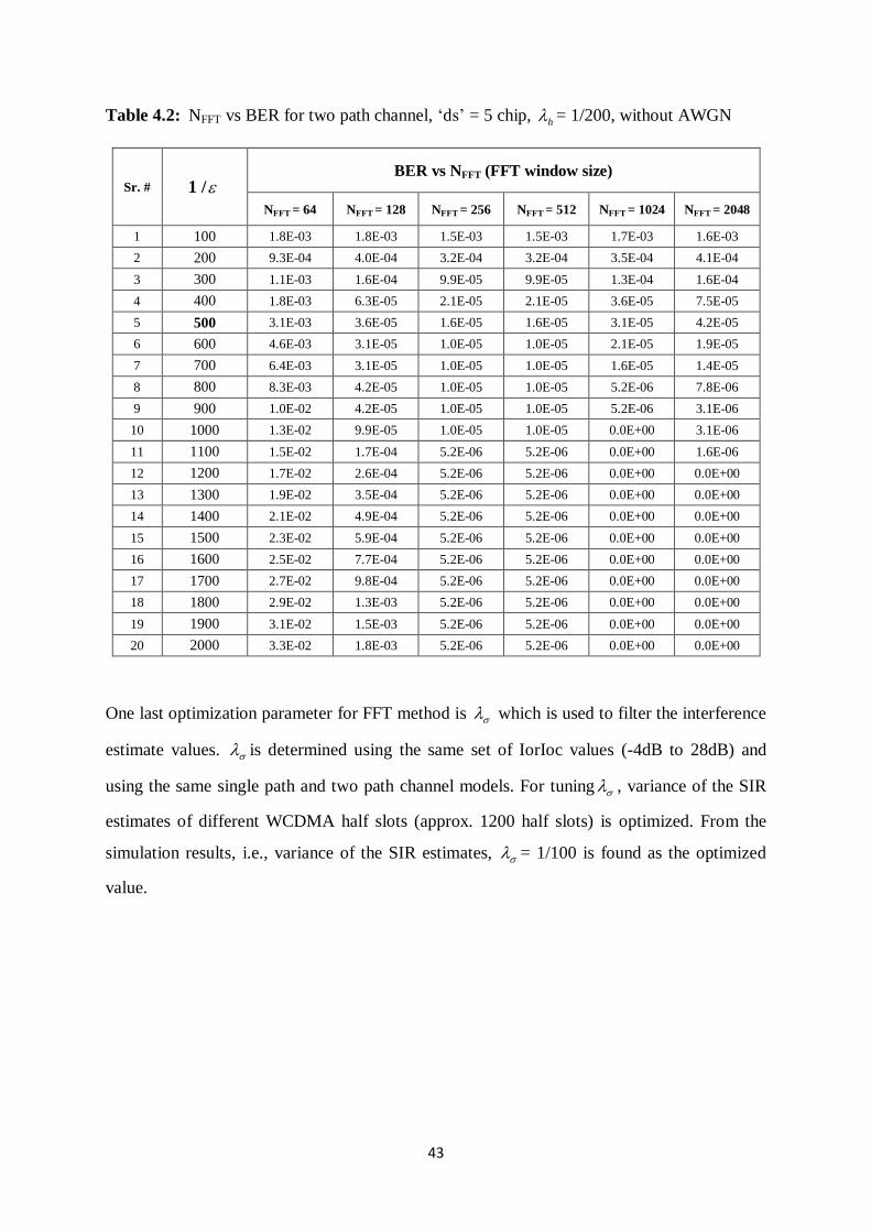
43
Table 4.2: NFFT vs BER for two path channel, „ds‟ = 5 chip, h = 1/200, without AWGN
Sr. # 1 / BER vs NFFT (FFT window size)
NFFT = 64 NFFT
= 128 NFFT
= 256 NFFT
= 512 NFFT
= 1024 NFFT
= 2048
1 100 1.8E-03 1.8E-03 1.5E-03 1.5E-03 1.7E-03 1.6E-03
2 200 9.3E-04 4.0E-04 3.2E-04 3.2E-04 3.5E-04 4.1E-04
3 300 1.1E-03 1.6E-04 9.9E-05 9.9E-05 1.3E-04 1.6E-04
4 400 1.8E-03 6.3E-05 2.1E-05 2.1E-05 3.6E-05 7.5E-05
5 500 3.1E-03 3.6E-05 1.6E-05 1.6E-05 3.1E-05 4.2E-05
6 600 4.6E-03 3.1E-05 1.0E-05 1.0E-05 2.1E-05 1.9E-05
7 700 6.4E-03 3.1E-05 1.0E-05 1.0E-05 1.6E-05 1.4E-05
8 800 8.3E-03 4.2E-05 1.0E-05 1.0E-05 5.2E-06 7.8E-06
9 900 1.0E-02 4.2E-05 1.0E-05 1.0E-05 5.2E-06 3.1E-06
10 1000 1.3E-02 9.9E-05 1.0E-05 1.0E-05 0.0E+00 3.1E-06
11 1100 1.5E-02 1.7E-04 5.2E-06 5.2E-06 0.0E+00 1.6E-06
12 1200 1.7E-02 2.6E-04 5.2E-06 5.2E-06 0.0E+00 0.0E+00
13 1300 1.9E-02 3.5E-04 5.2E-06 5.2E-06 0.0E+00 0.0E+00
14 1400 2.1E-02 4.9E-04 5.2E-06 5.2E-06 0.0E+00 0.0E+00
15 1500 2.3E-02 5.9E-04 5.2E-06 5.2E-06 0.0E+00 0.0E+00
16 1600 2.5E-02 7.7E-04 5.2E-06 5.2E-06 0.0E+00 0.0E+00
17 1700 2.7E-02 9.8E-04 5.2E-06 5.2E-06 0.0E+00 0.0E+00
18 1800 2.9E-02 1.3E-03 5.2E-06 5.2E-06 0.0E+00 0.0E+00
19 1900 3.1E-02 1.5E-03 5.2E-06 5.2E-06 0.0E+00 0.0E+00
20 2000 3.3E-02 1.8E-03 5.2E-06 5.2E-06 0.0E+00 0.0E+00
One last optimization parameter for FFT method is which is used to filter the interference
estimate values. is determined using the same set of IorIoc values (-4dB to 28dB) and
using the same single path and two path channel models. For tuning , variance of the SIR
estimates of different WCDMA half slots (approx. 1200 half slots) is optimized. From the
simulation results, i.e., variance of the SIR estimates, = 1/100 is found as the optimized
value.
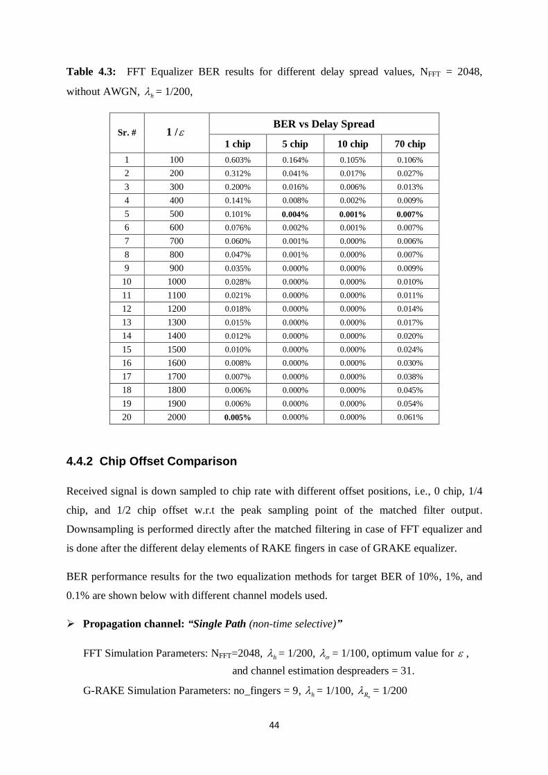
44
Table 4.3: FFT Equalizer BER results for different delay spread values, NFFT = 2048,
without AWGN, h = 1/200,
Sr. # 1 / BER vs Delay Spread
1 chip 5 chip 10 chip 70 chip
1 100 0.603% 0.164% 0.105% 0.106%
2 200 0.312% 0.041% 0.017% 0.027%
3 300 0.200% 0.016% 0.006% 0.013%
4 400 0.141% 0.008% 0.002% 0.009%
5 500 0.101% 0.004% 0.001% 0.007%
6 600 0.076% 0.002% 0.001% 0.007%
7 700 0.060% 0.001% 0.000% 0.006%
8 800 0.047% 0.001% 0.000% 0.007%
9 900 0.035% 0.000% 0.000% 0.009%
10 1000 0.028% 0.000% 0.000% 0.010%
11 1100 0.021% 0.000% 0.000% 0.011%
12 1200 0.018% 0.000% 0.000% 0.014%
13 1300 0.015% 0.000% 0.000% 0.017%
14 1400 0.012% 0.000% 0.000% 0.020%
15 1500 0.010% 0.000% 0.000% 0.024%
16 1600 0.008% 0.000% 0.000% 0.030%
17 1700 0.007% 0.000% 0.000% 0.038%
18 1800 0.006% 0.000% 0.000% 0.045%
19 1900 0.006% 0.000% 0.000% 0.054%
20 2000 0.005% 0.000% 0.000% 0.061%
4.4.2 Chip Offset Comparison
Received signal is down sampled to chip rate with different offset positions, i.e., 0 chip, 1/4
chip, and 1/2 chip offset w.r.t the peak sampling point of the matched filter output.
Downsampling is performed directly after the matched filtering in case of FFT equalizer and
is done after the different delay elements of RAKE fingers in case of GRAKE equalizer.
BER performance results for the two equalization methods for target BER of 10%, 1%, and
0.1% are shown below with different channel models used.
Propagation channel: “Single Path (non-time selective)”
FFT Simulation Parameters: NFFT=2048, h = 1/200, = 1/100, optimum value for ,
and channel estimation despreaders = 31.
G-RAKE Simulation Parameters: no_fingers = 9, h = 1/100, nR = 1/200
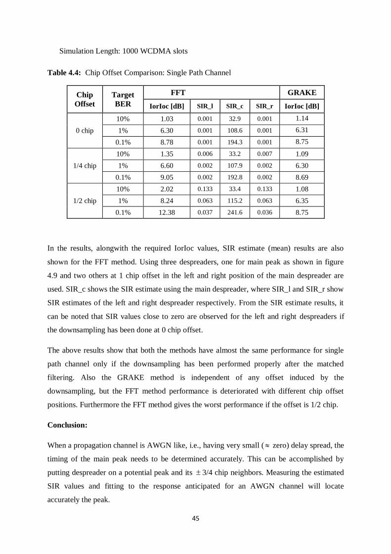
45
Simulation Length: 1000 WCDMA slots
Table 4.4: Chip Offset Comparison: Single Path Channel
Chip
Offset
Target
BER
FFT GRAKE
IorIoc [dB] SIR_l SIR_c SIR_r IorIoc [dB]
0 chip
10% 1.03 0.001 32.9 0.001 1.14
1% 6.30 0.001 108.6 0.001 6.31
0.1% 8.78 0.001 194.3 0.001 8.75
1/4 chip
10% 1.35 0.006 33.2 0.007 1.09
1% 6.60 0.002 107.9 0.002 6.30
0.1% 9.05 0.002 192.8 0.002 8.69
1/2 chip
10% 2.02 0.133 33.4 0.133 1.08
1% 8.24 0.063 115.2 0.063 6.35
0.1% 12.38 0.037 241.6 0.036 8.75
In the results, alongwith the required IorIoc values, SIR estimate (mean) results are also
shown for the FFT method. Using three despreaders, one for main peak as shown in figure
4.9 and two others at 1 chip offset in the left and right position of the main despreader are
used. SIR_c shows the SIR estimate using the main despreader, where SIR_l and SIR_r show
SIR estimates of the left and right despreader respectively. From the SIR estimate results, it
can be noted that SIR values close to zero are observed for the left and right despreaders if
the downsampling has been done at 0 chip offset.
The above results show that both the methods have almost the same performance for single
path channel only if the downsampling has been performed properly after the matched
filtering. Also the GRAKE method is independent of any offset induced by the
downsampling, but the FFT method performance is deteriorated with different chip offset
positions. Furthermore the FFT method gives the worst performance if the offset is 1/2 chip.
Conclusion:
When a propagation channel is AWGN like, i.e., having very small ( zero) delay spread, the
timing of the main peak needs to be determined accurately. This can be accomplished by
putting despreader on a potential peak and its 3/4 chip neighbors. Measuring the estimated
SIR values and fitting to the response anticipated for an AWGN channel will locate
accurately the peak.
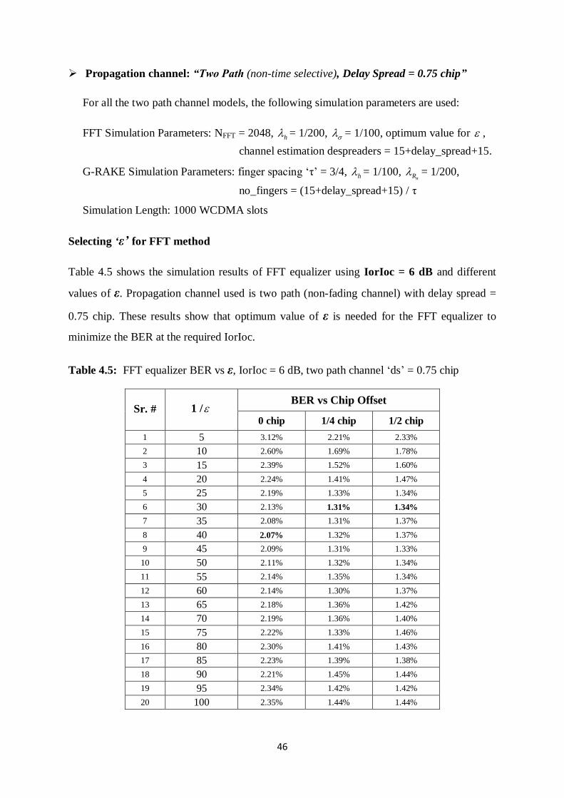
46
Propagation channel: “Two Path (non-time selective), Delay Spread = 0.75 chip”
For all the two path channel models, the following simulation parameters are used:
FFT Simulation Parameters: NFFT = 2048, h = 1/200, = 1/100, optimum value for ,
channel estimation despreaders = 15+delay_spread+15.
G-RAKE Simulation Parameters: finger spacing „τ‟ = 3/4, h = 1/100, nR = 1/200,
no_fingers = (15+delay_spread+15) / τ
Simulation Length: 1000 WCDMA slots
Selecting „ε‟ for FFT method
Table 4.5 shows the simulation results of FFT equalizer using IorIoc = 6 dB and different
values of ε. Propagation channel used is two path (non-fading channel) with delay spread =
0.75 chip. These results show that optimum value of ε is needed for the FFT equalizer to
minimize the BER at the required IorIoc.
Table 4.5: FFT equalizer BER vs ε, IorIoc = 6 dB, two path channel „ds‟ = 0.75 chip
Sr. # 1 / BER vs Chip Offset
0 chip 1/4 chip 1/2 chip
1 5 3.12% 2.21% 2.33%
2 10 2.60% 1.69% 1.78%
3 15 2.39% 1.52% 1.60%
4 20 2.24% 1.41% 1.47%
5 25 2.19% 1.33% 1.34%
6 30 2.13% 1.31% 1.34%
7 35 2.08% 1.31% 1.37%
8 40 2.07% 1.32% 1.37%
9 45 2.09% 1.31% 1.33%
10 50 2.11% 1.32% 1.34%
11 55 2.14% 1.35% 1.34%
12 60 2.14% 1.30% 1.37%
13 65 2.18% 1.36% 1.42%
14 70 2.19% 1.36% 1.40%
15 75 2.22% 1.33% 1.46%
16 80 2.30% 1.41% 1.43%
17 85 2.23% 1.39% 1.38%
18 90 2.21% 1.45% 1.44%
19 95 2.34% 1.42% 1.42%
20 100 2.35% 1.44% 1.44%
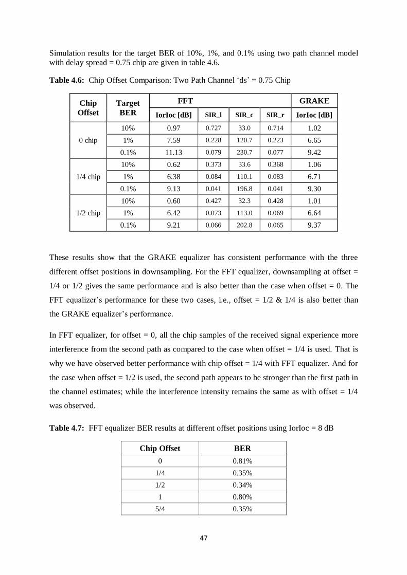
47
Simulation results for the target BER of 10%, 1%, and 0.1% using two path channel model
with delay spread = 0.75 chip are given in table 4.6.
Table 4.6: Chip Offset Comparison: Two Path Channel „ds‟ = 0.75 Chip
Chip
Offset
Target
BER
FFT GRAKE
IorIoc [dB] SIR_l SIR_c SIR_r IorIoc [dB]
0 chip
10% 0.97 0.727 33.0 0.714 1.02
1% 7.59 0.228 120.7 0.223 6.65
0.1% 11.13 0.079 230.7 0.077 9.42
1/4 chip
10% 0.62 0.373 33.6 0.368 1.06
1% 6.38 0.084 110.1 0.083 6.71
0.1% 9.13 0.041 196.8 0.041 9.30
1/2 chip
10% 0.60 0.427 32.3 0.428 1.01
1% 6.42 0.073 113.0 0.069 6.64
0.1% 9.21 0.066 202.8 0.065 9.37
These results show that the GRAKE equalizer has consistent performance with the three
different offset positions in downsampling. For the FFT equalizer, downsampling at offset =
1/4 or 1/2 gives the same performance and is also better than the case when offset = 0. The
FFT equalizer‟s performance for these two cases, i.e., offset = 1/2 & 1/4 is also better than
the GRAKE equalizer‟s performance.
In FFT equalizer, for offset = 0, all the chip samples of the received signal experience more
interference from the second path as compared to the case when offset = 1/4 is used. That is
why we have observed better performance with chip offset = 1/4 with FFT equalizer. And for
the case when offset = 1/2 is used, the second path appears to be stronger than the first path in
the channel estimates; while the interference intensity remains the same as with offset = 1/4
was observed.
Table 4.7: FFT equalizer BER results at different offset positions using IorIoc = 8 dB
Chip Offset BER
0 0.81%
1/4 0.35%
1/2 0.34%
1 0.80%
5/4 0.35%
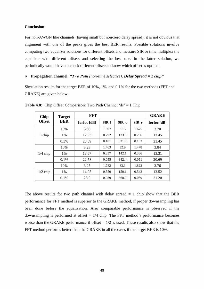
48
Conclusion:
For non-AWGN like channels (having small but non-zero delay spread), it is not obvious that
alignment with one of the peaks gives the best BER results. Possible solutions involve
computing two equalizer solutions for different offsets and measure SIR or time multiplex the
equalizer with different offsets and selecting the best one. In the latter solution, we
periodically would have to check different offsets to know which offset is optimal.
Propagation channel: “Two Path (non-time selective), Delay Spread = 1 chip”
Simulation results for the target BER of 10%, 1%, and 0.1% for the two methods (FFT and
GRAKE) are given below:
Table 4.8: Chip Offset Comparison: Two Path Channel „ds‟ = 1 Chip
Chip
Offset
Target
BER
FFT GRAKE
IorIoc [dB] SIR_l SIR_c SIR_r IorIoc [dB]
0 chip
10% 3.08 1.697 31.5 1.675 3.70
1% 12.93 0.292 133.8 0.286 13.45
0.1% 20.09 0.101 321.8 0.102 21.45
1/4 chip
10% 3.23 1.463 32.9 1.478 3.84
1% 13.67 0.357 142.1 0.366 13.31
0.1% 22.58 0.055 342.4 0.051 20.69
1/2 chip
10% 3.25 1.782 33.1 1.822 3.76
1% 14.95 0.550 150.1 0.542 13.52
0.1% 28.0 0.089 368.0 0.089 21.20
The above results for two path channel with delay spread = 1 chip show that the BER
performance for FFT method is superior to the GRAKE method, if proper downsampling has
been done before the equalization. Also comparable performance is observed if the
downsampling is performed at offset = 1/4 chip. The FFT method‟s performance becomes
worse than the GRAKE performance if offset = 1/2 is used. These results also show that the
FFT method performs better than the GRAKE in all the cases if the target BER is 10%.
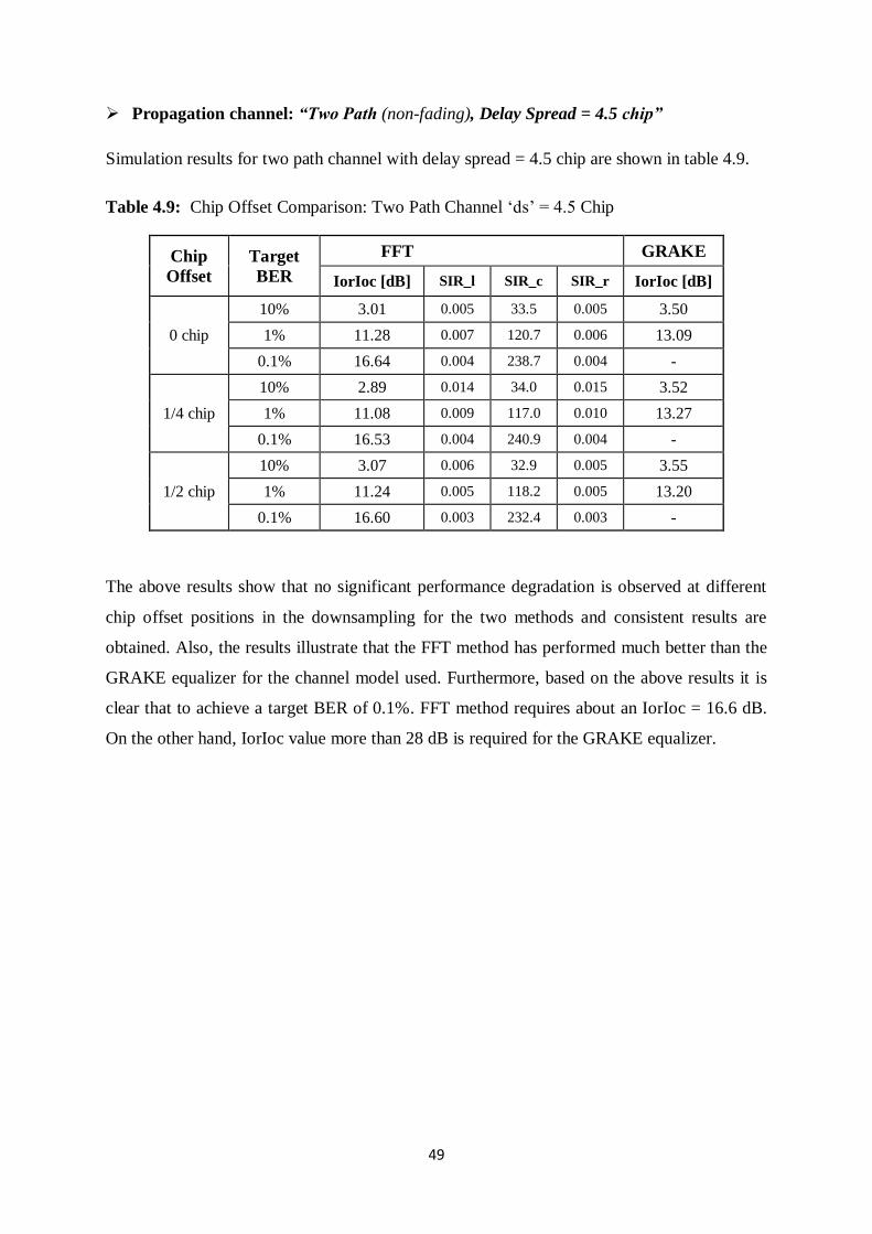
49
Propagation channel: “Two Path (non-fading), Delay Spread = 4.5 chip”
Simulation results for two path channel with delay spread = 4.5 chip are shown in table 4.9.
Table 4.9: Chip Offset Comparison: Two Path Channel „ds‟ = 4.5 Chip
Chip
Offset
Target
BER
FFT GRAKE
IorIoc [dB] SIR_l SIR_c SIR_r IorIoc [dB]
0 chip
10% 3.01 0.005 33.5 0.005 3.50
1% 11.28 0.007 120.7 0.006 13.09
0.1% 16.64 0.004 238.7 0.004 -
1/4 chip
10% 2.89 0.014 34.0 0.015 3.52
1% 11.08 0.009 117.0 0.010 13.27
0.1% 16.53 0.004 240.9 0.004 -
1/2 chip
10% 3.07 0.006 32.9 0.005 3.55
1% 11.24 0.005 118.2 0.005 13.20
0.1% 16.60 0.003 232.4 0.003 -
The above results show that no significant performance degradation is observed at different
chip offset positions in the downsampling for the two methods and consistent results are
obtained. Also, the results illustrate that the FFT method has performed much better than the
GRAKE equalizer for the channel model used. Furthermore, based on the above results it is
clear that to achieve a target BER of 0.1%. FFT method requires about an IorIoc = 16.6 dB.
On the other hand, IorIoc value more than 28 dB is required for the GRAKE equalizer.
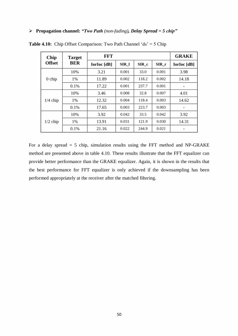
50
Propagation channel: “Two Path (non-fading), Delay Spread = 5 chip”
Table 4.10: Chip Offset Comparison: Two Path Channel „ds‟ = 5 Chip
Chip
Offset
Target
BER
FFT GRAKE
IorIoc [dB] SIR_l SIR_c SIR_r IorIoc [dB]
0 chip
10% 3.21 0.001 33.0 0.001 3.98
1% 11.89 0.002 118.2 0.002 14.18
0.1% 17.22 0.001 237.7 0.001 -
1/4 chip
10% 3.46 0.008 32.8 0.007 4.01
1% 12.32 0.004 118.4 0.003 14.62
0.1% 17.65 0.003 223.7 0.003 -
1/2 chip
10% 3.92 0.042 33.5 0.042 3.92
1% 13.91 0.031 121.9 0.030 14.31
0.1% 21.16 0.022 244.9 0.021 -
For a delay spread = 5 chip, simulation results using the FFT method and NP-GRAKE
method are presented above in table 4.10. These results illustrate that the FFT equalizer can
provide better performance than the GRAKE equalizer. Again, it is shown in the results that
the best performance for FFT equalizer is only achieved if the downsampling has been
performed appropriately at the receiver after the matched filtering.
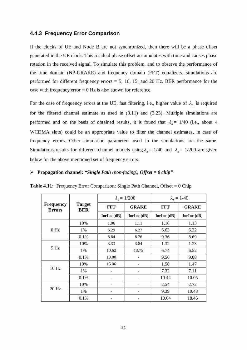
51
4.4.3 Frequency Error Comparison
If the clocks of UE and Node B are not synchronized, then there will be a phase offset
generated in the UE clock. This residual phase offset accumulates with time and causes phase
rotation in the received signal. To simulate this problem, and to observe the performance of
the time domain (NP-GRAKE) and frequency domain (FFT) equalizers, simulations are
performed for different frequency errors = 5, 10, 15, and 20 Hz. BER performance for the
case with frequency error = 0 Hz is also shown for reference.
For the case of frequency errors at the UE, fast filtering, i.e., higher value of h is required
for the filtered channel estimate as used in (3.11) and (3.23). Multiple simulations are
performed and on the basis of obtained results, it is found that h = 1/40 (i.e., about 4
WCDMA slots) could be an appropriate value to filter the channel estimates, in case of
frequency errors. Other simulation parameters used in the simulations are the same.
Simulations results for different channel models using h = 1/40 and h = 1/200 are given
below for the above mentioned set of frequency errors.
Propagation channel: “Single Path (non-fading), Offset = 0 chip”
Table 4.11: Frequency Error Comparison: Single Path Channel, Offset = 0 Chip
Frequency
Errors
Target
BER
h = 1/200 h = 1/40
FFT GRAKE FFT GRAKE
IorIoc [dB] IorIoc [dB] IorIoc [dB] IorIoc [dB]
0 Hz
10% 1.06 1.11 1.18 1.13
1% 6.29 6.27 6.63 6.32
0.1% 8.84 8.76 9.36 8.69
5 Hz 10% 3.33 3.84 1.32 1.23
1% 10.62 13.75 6.74 6.52
0.1% 13.80 - 9.56 9.08
10 Hz 10% 15.06 - 1.58 1.47
1% - - 7.32 7.11
0.1% - - 10.44 10.05
20 Hz 10% - - 2.54 2.72
1% - - 9.39 10.43
0.1% - - 13.04 18.45
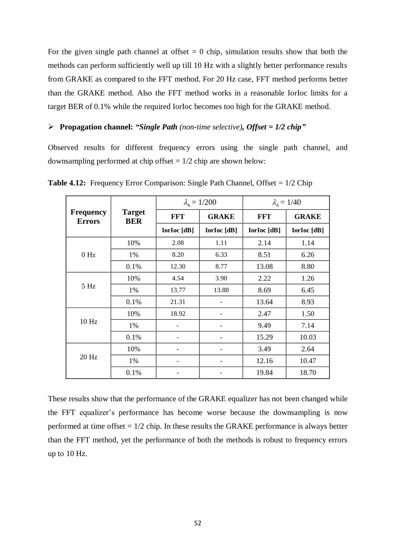
52
For the given single path channel at offset = 0 chip, simulation results show that both the
methods can perform sufficiently well up till 10 Hz with a slightly better performance results
from GRAKE as compared to the FFT method. For 20 Hz case, FFT method performs better
than the GRAKE method. Also the FFT method works in a reasonable IorIoc limits for a
target BER of 0.1% while the required IorIoc becomes too high for the GRAKE method.
Propagation channel: “Single Path (non-time selective), Offset = 1/2 chip”
Observed results for different frequency errors using the single path channel, and
downsampling performed at chip offset = 1/2 chip are shown below:
Table 4.12: Frequency Error Comparison: Single Path Channel, Offset = 1/2 Chip
Frequency
Errors
Target
BER
h = 1/200 h = 1/40
FFT GRAKE FFT GRAKE
IorIoc [dB] IorIoc [dB] IorIoc [dB] IorIoc [dB]
0 Hz
10% 2.08 1.11 2.14 1.14
1% 8.20 6.33 8.51 6.26
0.1% 12.30 8.77 13.08 8.80
5 Hz 10% 4.54 3.90 2.22 1.26
1% 13.77 13.88 8.69 6.45
0.1% 21.31 - 13.64 8.93
10 Hz 10% 18.92 - 2.47 1.50
1% - - 9.49 7.14
0.1% - - 15.29 10.03
20 Hz 10% - - 3.49 2.64
1% - - 12.16 10.47
0.1% - - 19.84 18.70
These results show that the performance of the GRAKE equalizer has not been changed while
the FFT equalizer‟s performance has become worse because the downsampling is now
performed at time offset = 1/2 chip. In these results the GRAKE performance is always better
than the FFT method, yet the performance of both the methods is robust to frequency errors
up to 10 Hz.
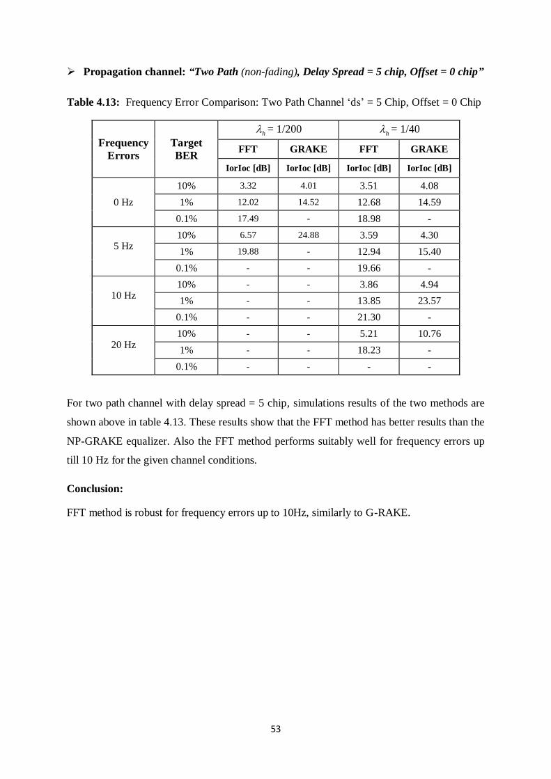
53
Propagation channel: “Two Path (non-fading), Delay Spread = 5 chip, Offset = 0 chip”
Table 4.13: Frequency Error Comparison: Two Path Channel „ds‟ = 5 Chip, Offset = 0 Chip
Frequency
Errors
Target
BER
h = 1/200 h = 1/40
FFT GRAKE FFT GRAKE
IorIoc [dB] IorIoc [dB] IorIoc [dB] IorIoc [dB]
0 Hz
10% 3.32 4.01 3.51 4.08
1% 12.02 14.52 12.68 14.59
0.1% 17.49 - 18.98 -
5 Hz 10% 6.57 24.88 3.59 4.30
1% 19.88 - 12.94 15.40
0.1% - - 19.66 -
10 Hz 10% - - 3.86 4.94
1% - - 13.85 23.57
0.1% - - 21.30 -
20 Hz 10% - - 5.21 10.76
1% - - 18.23 -
0.1% - - - -
For two path channel with delay spread = 5 chip, simulations results of the two methods are
shown above in table 4.13. These results show that the FFT method has better results than the
NP-GRAKE equalizer. Also the FFT method performs suitably well for frequency errors up
till 10 Hz for the given channel conditions.
Conclusion:
FFT method is robust for frequency errors up to 10Hz, similarly to G-RAKE.
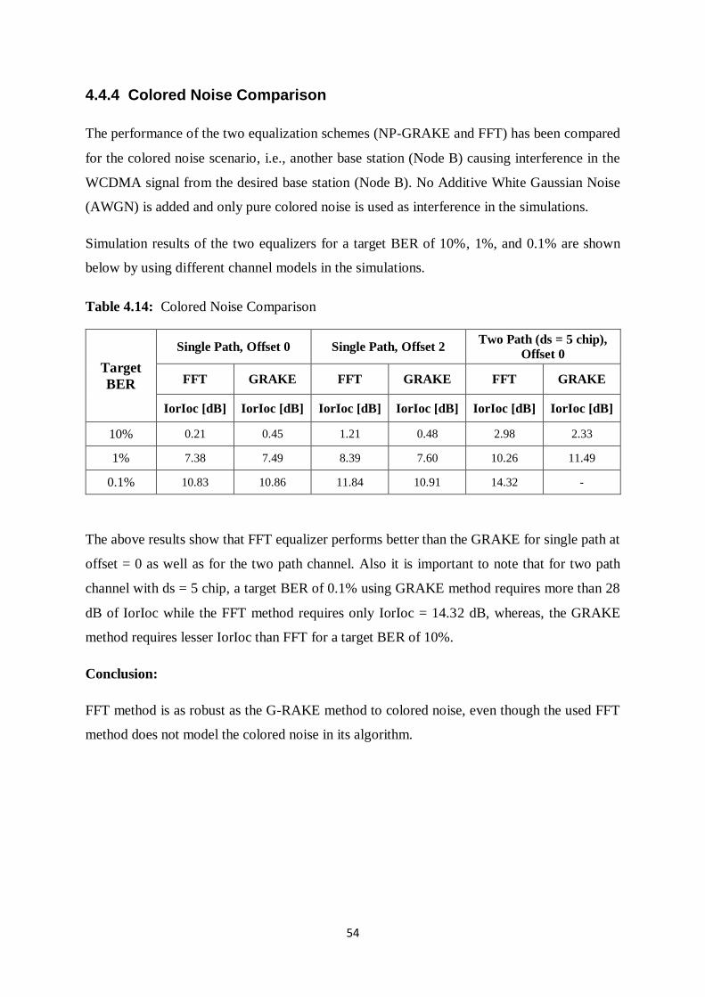
54
4.4.4 Colored Noise Comparison
The performance of the two equalization schemes (NP-GRAKE and FFT) has been compared
for the colored noise scenario, i.e., another base station (Node B) causing interference in the
WCDMA signal from the desired base station (Node B). No Additive White Gaussian Noise
(AWGN) is added and only pure colored noise is used as interference in the simulations.
Simulation results of the two equalizers for a target BER of 10%, 1%, and 0.1% are shown
below by using different channel models in the simulations.
Table 4.14: Colored Noise Comparison
Target
BER
Single Path, Offset 0 Single Path, Offset 2 Two Path (ds = 5 chip),
Offset 0
FFT GRAKE FFT GRAKE FFT GRAKE
IorIoc [dB] IorIoc [dB] IorIoc [dB] IorIoc [dB] IorIoc [dB] IorIoc [dB]
10% 0.21 0.45 1.21 0.48 2.98 2.33
1% 7.38 7.49 8.39 7.60 10.26 11.49
0.1% 10.83 10.86 11.84 10.91 14.32 -
The above results show that FFT equalizer performs better than the GRAKE for single path at
offset = 0 as well as for the two path channel. Also it is important to note that for two path
channel with ds = 5 chip, a target BER of 0.1% using GRAKE method requires more than 28
dB of IorIoc while the FFT method requires only IorIoc = 14.32 dB, whereas, the GRAKE
method requires lesser IorIoc than FFT for a target BER of 10%.
Conclusion:
FFT method is as robust as the G-RAKE method to colored noise, even though the used FFT
method does not model the colored noise in its algorithm.
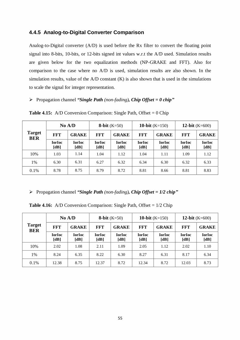
55
4.4.5 Analog-to-Digital Converter Comparison
Analog-to-Digital converter (A/D) is used before the Rx filter to convert the floating point
signal into 8-bits, 10-bits, or 12-bits signed int values w.r.t the A/D used. Simulation results
are given below for the two equalization methods (NP-GRAKE and FFT). Also for
comparison to the case where no A/D is used, simulation results are also shown. In the
simulation results, value of the A/D constant (K) is also shown that is used in the simulations
to scale the signal for integer representation.
Propagation channel “Single Path (non-fading), Chip Offset = 0 chip”
Table 4.15: A/D Conversion Comparison: Single Path, Offset = 0 Chip
Target
BER
No A/D 8-bit (K=50) 10-bit (K=150) 12-bit (K=600)
FFT GRAKE FFT GRAKE FFT GRAKE FFT GRAKE
IorIoc
[dB]
IorIoc
[dB]
IorIoc
[dB]
IorIoc
[dB]
IorIoc
[dB]
IorIoc
[dB]
IorIoc
[dB]
IorIoc
[dB]
10% 1.03 1.14 1.04 1.12 1.04 1.11 1.09 1.12
1% 6.30 6.31 6.27 6.32 6.34 6.30 6.32 6.33
0.1% 8.78 8.75 8.79 8.72 8.81 8.66 8.81 8.83
Propagation channel “Single Path (non-fading), Chip Offset = 1/2 chip”
Table 4.16: A/D Conversion Comparison: Single Path, Offset = 1/2 Chip
Target
BER
No A/D 8-bit (K=50) 10-bit (K=150) 12-bit (K=600)
FFT GRAKE FFT GRAKE FFT GRAKE FFT GRAKE
IorIoc
[dB]
IorIoc
[dB]
IorIoc
[dB]
IorIoc
[dB]
IorIoc
[dB]
IorIoc
[dB]
IorIoc
[dB]
IorIoc
[dB]
10% 2.02 1.08 2.11 1.09 2.05 1.12 2.02 1.10
1% 8.24 6.35 8.22 6.30 8.27 6.31 8.17 6.34
0.1% 12.38 8.75 12.37 8.72 12.34 8.72 12.03 8.73
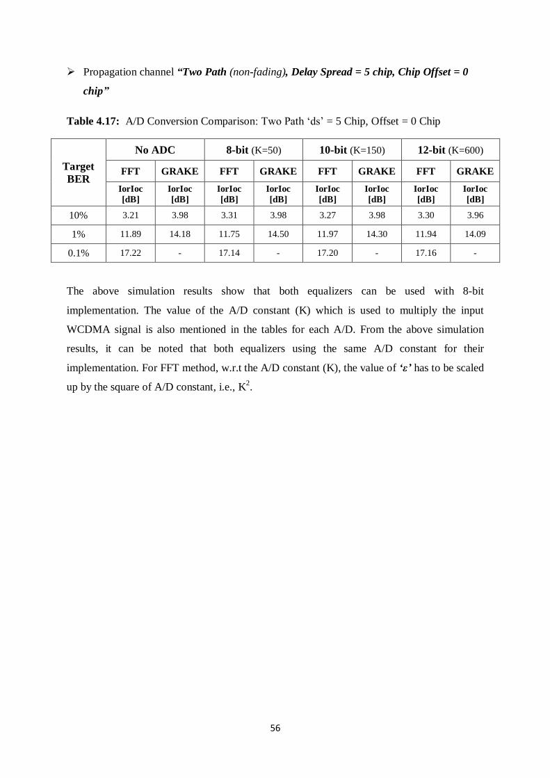
56
Propagation channel “Two Path (non-fading), Delay Spread = 5 chip, Chip Offset = 0
chip”
Table 4.17: A/D Conversion Comparison: Two Path „ds‟ = 5 Chip, Offset = 0 Chip
Target
BER
No ADC 8-bit (K=50) 10-bit (K=150) 12-bit (K=600)
FFT GRAKE FFT GRAKE FFT GRAKE FFT GRAKE
IorIoc
[dB]
IorIoc
[dB]
IorIoc
[dB]
IorIoc
[dB]
IorIoc
[dB]
IorIoc
[dB]
IorIoc
[dB]
IorIoc
[dB]
10% 3.21 3.98 3.31 3.98 3.27 3.98 3.30 3.96
1% 11.89 14.18 11.75 14.50 11.97 14.30 11.94 14.09
0.1% 17.22 - 17.14 - 17.20 - 17.16 -
The above simulation results show that both equalizers can be used with 8-bit
implementation. The value of the A/D constant (K) which is used to multiply the input
WCDMA signal is also mentioned in the tables for each A/D. From the above simulation
results, it can be noted that both equalizers using the same A/D constant for their
implementation. For FFT method, w.r.t the A/D constant (K), the value of „ε‟ has to be scaled
up by the square of A/D constant, i.e., K2.
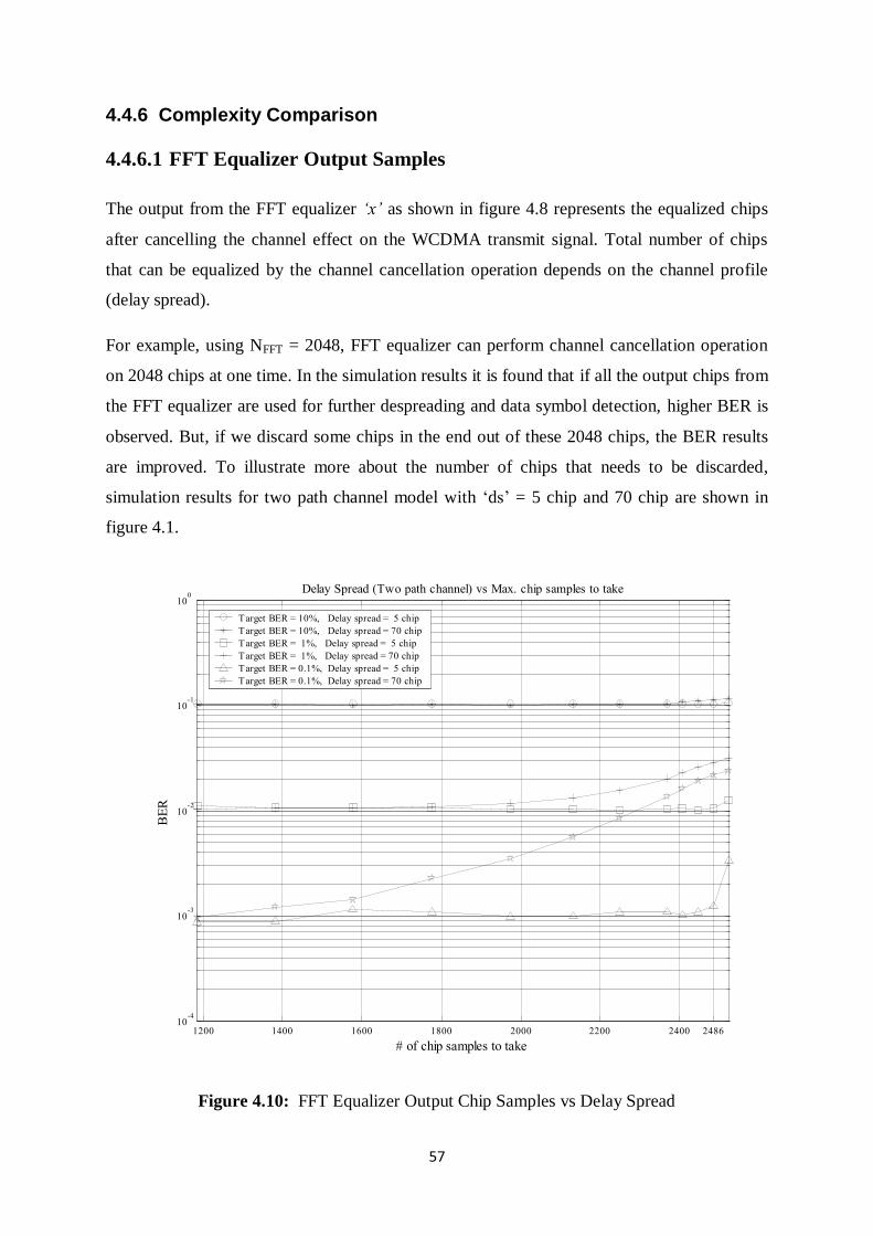
57
4.4.6 Complexity Comparison
4.4.6.1 FFT Equalizer Output Samples
The output from the FFT equalizer „x‟ as shown in figure 4.8 represents the equalized chips
after cancelling the channel effect on the WCDMA transmit signal. Total number of chips
that can be equalized by the channel cancellation operation depends on the channel profile
(delay spread).
For example, using NFFT = 2048, FFT equalizer can perform channel cancellation operation
on 2048 chips at one time. In the simulation results it is found that if all the output chips from
the FFT equalizer are used for further despreading and data symbol detection, higher BER is
observed. But, if we discard some chips in the end out of these 2048 chips, the BER results
are improved. To illustrate more about the number of chips that needs to be discarded,
simulation results for two path channel model with „ds‟ = 5 chip and 70 chip are shown in
figure 4.1.
Figure 4.10: FFT Equalizer Output Chip Samples vs Delay Spread
1200 1400 1600 1800 2000 2200 2400 248610
-4
10-3
10-2
10-1
100
# of chip samples to take
BE
R
Delay Spread (Two path channel) vs Max. chip samples to take
Target BER = 10%, Delay spread = 5 chip
Target BER = 10%, Delay spread = 70 chip
Target BER = 1%, Delay spread = 5 chip
Target BER = 1%, Delay spread = 70 chip
Target BER = 0.1%, Delay spread = 5 chip
Target BER = 0.1%, Delay spread = 70 chip
58
The simulation results show that, for FFT equalizer, the number of chips that are equalized in
a WCDMA slot depends on the channel profile (delay spread). Also, the simulations results
show that depending on the target BER output chip samples that can be retained are different.
For a target BER of 10%, even with a delay spread of 70 chips, all the 2560 output chips can
be used for despreading. But for a target BER of 0.1%, and delay spread = 70 chips, number
of chip samples to take are about half of the output samples, i.e., 1280 chips. Similarly the
above results show that, for a delay spread = 5 chip and target BER of 1% and 0.1%, about 80
chips can be discarded out of 2560 chips while others can be used for despreading and
symbol detection.
Now, by using a two path channel with delay spread = 5 chip, in order to process one
WCDMA slot complexity comparison for the two equalization schemes is done based on the
following computations
CPICH channel generation
Equalizer weights generation for NP-GRAKE or FFT method
FFT and IFFT
Data demodulation
Assuming that the number of despreaders used for the CPICH channel estimates are same for
the two equalization methods. For a two path channel with delay spread = 5 chip, the number
of despreaders required for channels estimate = 15+delay_spread+15 = 35 despreaders.
The complexity comparison will be based on the total number of complex operations required
for the two equalizers. In general, we will refer to the different arithmetic operations such as
multiplication, division, addition, or subtraction as a complex operation.
4.4.6.2 Computations For FFT
Total complex operations required for CPICH channel generation using FFT method is given
as
35*(256+256+256+1)*10 + (35+35+35)*10 = 270,200
where first 256 operations represent the scrambling code multiplications, second 256
operations are for channelization code and third 256 operations are for the summation
operation following these multiplications. One division operation is added for CPICH pilot
symbol division. Total 35 despreaders are used for channel values estimation. Then the other
59
operations are used for the filtering operation which is performed on the current channel
values and filtered channel values
Total complex operations for an FFT are calculated using the classic Cooley-Tukey method.
For a radix-2 algorithm, total complex multiplication required are ~ (NFFT/2)*log2(NFFT) and
total complex additions are (NFFT)*log2(NFFT), where NFFT is the size of the FFT used [9].
After adding other operations to compute the FFT equalizer numerator and denominator
values, using NFFT = 2048, total operations required to calculate the FFT equalizer filter are
(NFFT+ NFFT/2)*log2(NFFT) + (NFFT+ NFFT+ NFFT) = 37,888
Computations done for taking the FFT of the input signal and the IFFT of the equalized
signal are given below
(NFFT+ NFFT/2)*log2(NFFT) + NFFT + (NFFT+ NFFT/2)*log2(NFFT) = 69,632
„M‟ Equalized chips are taken out based on the decision output from the intelligent block of
FFT equalizer. For a delay spread = 5 chip, using NFFT = 2048, „M‟ = 1984 chips out of 2048
can be retained after equalization. The computations required to detect the data symbols using
the descrambling and despreading operations are then
M+M+M = 5,952
4.4.6.3 Computations for NP-GRAKE
Total complex operations required for CPICH channel generation using NP-GRAKE method
are given below, which are the same as for the FFT method
35*(256+256+256+1)*10 + (35+35+35)*10 = 270,200
The computations required for calculating the noise covariance matrix and further the matrix
inversion are determined using the Cholesky based algorithm [10]. Matrix inversion
operation is performed once per WCDMA slot and noise covariance matrix is computed 10
times based on the sample channel estimate values. As the covariance matrix is symmetric,
total operations are also divided by 2 in the following expression. By including the filtering
operation, the number of computations required to get the equalizer filter weights for NP-
GRAKE equalizer are:
no_fing3 / 3 + 2*no_fing
2 + (no_fing
2+no_fing
2+no_fing
2+no_fing
2)*(10/2) = 41,242
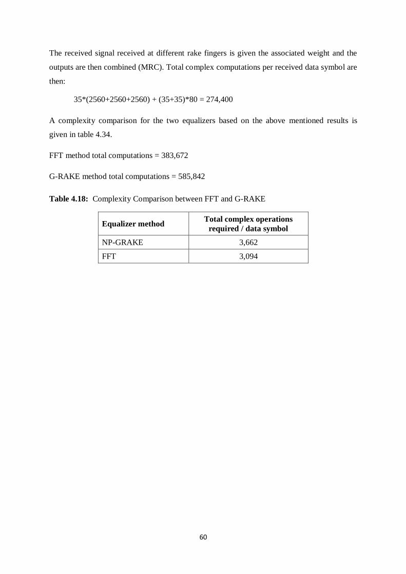
60
The received signal received at different rake fingers is given the associated weight and the
outputs are then combined (MRC). Total complex computations per received data symbol are
then:
35*(2560+2560+2560) + (35+35)*80 = 274,400
A complexity comparison for the two equalizers based on the above mentioned results is
given in table 4.34.
FFT method total computations = 383,672
G-RAKE method total computations = 585,842
Table 4.18: Complexity Comparison between FFT and G-RAKE
Equalizer method Total complex operations
required / data symbol
NP-GRAKE 3,662
FFT 3,094
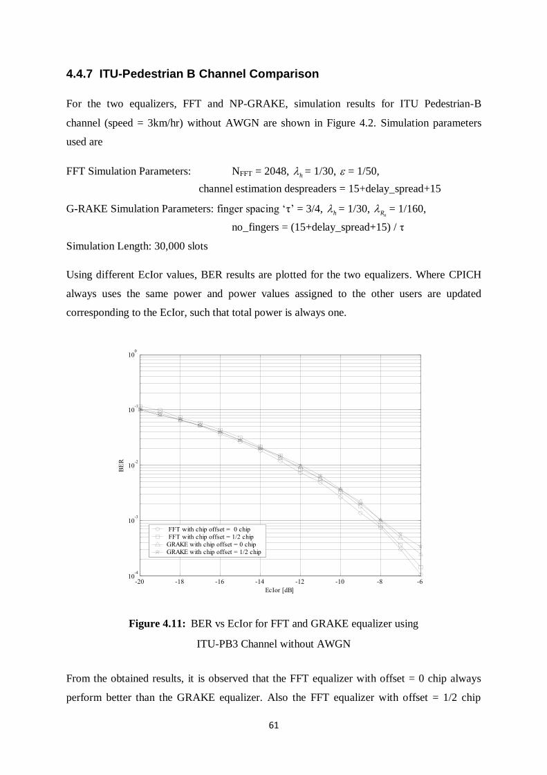
61
4.4.7 ITU-Pedestrian B Channel Comparison
For the two equalizers, FFT and NP-GRAKE, simulation results for ITU Pedestrian-B
channel (speed = 3km/hr) without AWGN are shown in Figure 4.2. Simulation parameters
used are
FFT Simulation Parameters: NFFT = 2048, h = 1/30, = 1/50,
channel estimation despreaders = 15+delay_spread+15
G-RAKE Simulation Parameters: finger spacing „τ‟ = 3/4, h = 1/30, nR = 1/160,
no_fingers = (15+delay_spread+15) / τ
Simulation Length: 30,000 slots
Using different EcIor values, BER results are plotted for the two equalizers. Where CPICH
always uses the same power and power values assigned to the other users are updated
corresponding to the EcIor, such that total power is always one.
Figure 4.11: BER vs EcIor for FFT and GRAKE equalizer using
ITU-PB3 Channel without AWGN
From the obtained results, it is observed that the FFT equalizer with offset = 0 chip always
perform better than the GRAKE equalizer. Also the FFT equalizer with offset = 1/2 chip
-20 -18 -16 -14 -12 -10 -8 -610
-4
10-3
10-2
10-1
100
EcIor [dB]
BE
R
FFT with chip offset = 0 chip
FFT with chip offset = 1/2 chip
GRAKE with chip offset = 0 chip
GRAKE with chip offset = 1/2 chip
62
performs better than the GRAKE equalizer if the desired user have more power assigned.
From the results it can be noted that if EcIor is in the range of -12 to -6 dB, then the FFT
equalizer is better than the G-RAKE equalizer even if the chip offset = 1/2 chip.

63
Chapter 5
5 Conclusion
In this thesis, we have investigated two equalization schemes for WCDMA. One is time
domain equalization using ML-based Non-parametric G-RAKE method and the other is
frequency domain equalization using FFT method. A simulator is made in IT++ and un-
coded BER results are used to compare the performance of these two equalizers.
BER performance results for different time offset (0, ¼, ½ chip) received signals are
compared. From the observed results, it is found that the performance of FFT based equalizer
is better than the G-RAKE equalizer for large delay spread channels. Also, the FFT equalizer
has comparable performance to the G-RAKE equalizer for small delay spread channels. It is
found that, the G-RAKE equalizer performance is not affected by the different time offset
received signals, but, the FFT equalizer has varied performance results. For FFT method, the
timing of the main peak needs to be determined accurately for small delay spread channels;
and for larger delay spread channels, two equalizer solution might be required by measuring
the SIR estimate for two different offsets and selecting the one with highest SIR estimate.
The performance of the two equalizer methods is also compared for different frequency
errors generated at the UE. From the obtained results, it is found that both the equalizers are
robust to frequency errors at UE, up-to 10 Hz. Simulation results for colored noise
(interference from another Node B) show that the FFT equalizer is as robust to colored noise
as the G-RAKE method even though the used FFT method does not model colored noise in
its algorithm. Also, for analog-to-digital conversion, quantization issues are observed for
different fixed point implementations and it is concluded that the FFT method can be used
with 8-bit ADC implementation. Total complex operations required per data symbol for FFT
and G-RAKE method are determined and it is found that the computations required for FFT
method are lesser as compared to the G-RAKE method.
Also, in this thesis, a comparison is shown between FFT and G-RAKE method using ITU-
Pedestrian B channel with speed = 3km/hr and frequency = 2.0 GHz. Simulations are
64
performed using different EcIor values and without AWGN. From the observed results, it is
found that the FFT method has better performance than the G-RAKE equalizer for fading and
multi-path channel conditions.
In the simulation results it is also observed that, for FFT equalizer, the number of chips
output from the equalizer depend on the delay spread. For small delay spread channels almost
all the chips in the FFT window are equalized but for medium to larger delay spread
channels, lesser chips can be retained at the equalizer output for subsequent despreading and
data symbol detection.
Future studies can be performed to optimally place the FFT grid on the input signal to get
higher throughput with minimum BER. In the future work, FFT equalizer can be
implemented with fixed point implementation for propagation channels with higher Doppler
frequencies. Smaller FFT window size will be required at higher velocities as the propagation
channels needs to be constant over an FFT window.
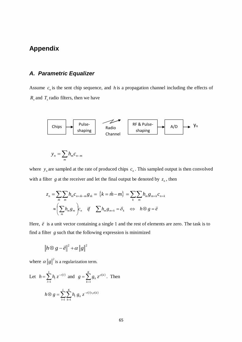
65
Appendix
A. Parametric Equalizer
Assume nc is the sent chip sequence, and h is a propagation channel including the effects of
xR and xT radio filters, then we have
m
mnmn chy
where ny are sampled at the rate of produced chips nc . This sampled output is then convolved
with a filter g at the receiver and let the final output be denoted by nz , then
k m
knkmm
m m
mmmnmn cghmmkgchz ˆˆ
ˆˆ
eghghifcgh kkmmn
m
mm
Here, e
is a unit vector containing a single 1 and the rest of elements are zero. The task is to
find a filter g such that the following expression is minimized
22
gegh
where 2
g is a regularization term.
Let
L
l
l
l zhh1
and
K
k
k
k zgg1
. Then
L
l
kl
k
K
k
l zghgh1 1
Radio
Channel
Chips Pulse-
shaping
RF & Pulse-
shaping A/D yn
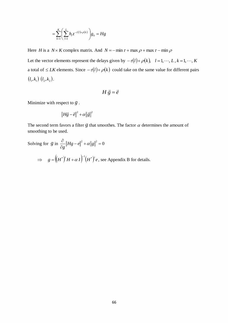
66
Hggzh k
K
k
klL
l
l
1 1
Here H is a KN complex matrix. And minmaxmaxmin N
Let the vector elements represent the delays given by KkLlkl ,,1,,,1,
a total of LK elements. Since kl could take on the same value for different pairs
2211 ,, klkl .
egH
Minimize with respect to g .
22
gegH
The second term favors a filter g that smoothes. The factor determines the amount of
smoothing to be used.
Solving for g in 022
geHg
g
eHIHHgtt *
1*
, see Appendix B for details.
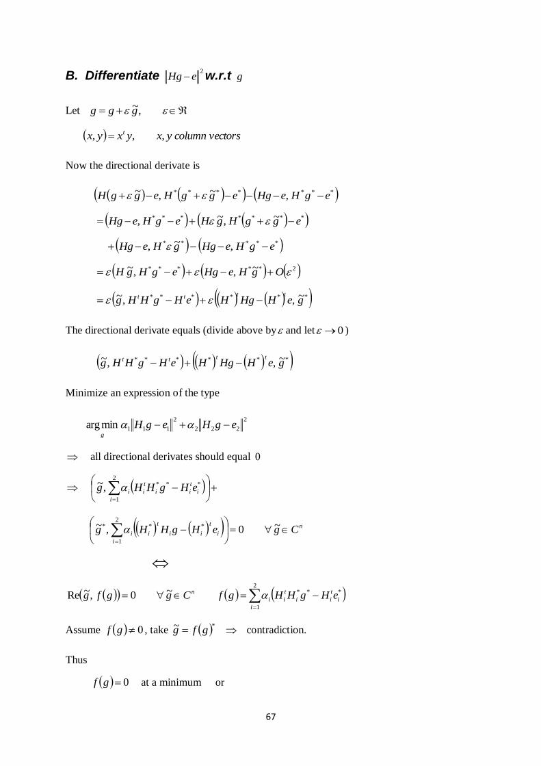
67
B. Differentiate 2
eHg w.r.t g
Let ,~ggg
vectorscolumnyxyxyx t ,,,
Now the directional derivate is
******* ,~,~ egHeHgeggHeggH
******* ~,~, eggHgHegHeHg
***** ,~, egHeHggHeHg
2***** ~,,~ OgHeHgegHgH
****** ~,,~ geHHgHeHgHHgtttt
The directional derivate equals (divide above by and let 0 )
****** ~,,~ geHHgHeHgHHgtttt
Minimize an expression of the type
2
222
2
111minarg egHegHg
all directional derivates should equal 0
2
1
***,~
i
i
t
ii
t
ii eHgHHg
n
i
i
t
ii
t
ii CgeHgHHg
~0,~2
1
***
2
1
***~0,~Rei
i
t
ii
t
ii
n eHgHHgfCggfg
Assume 0gf , take *~ gfg contradiction.
Thus
0gf at a minimum or
68
02
1
**
i
i
t
ii
t
ii eHgHH
2
1
*
12
1
*
i
i
t
i
i
i
t
ii eHHHg
69
References
[1] Andreas F. Molish, Wireless Communications, John Wiley & Sons, England, 2005.
[2] John G. Proakis, Digital Communications, Fourth Edition, McGraw-Hill, 2001
[3] Harri Holma and Antti Toskala, WCDMA for UMTS, Radio Access for Third
Generation Mobile Communications, Third Edition, John Wiley & Sons, England,
2004.
[4] Andrew Richardson, WCDMA Design Handbook, Cambridge University Press, 2005.
[5] Viterbi, A., Principles of Spread Spectrum Communication, Addison-Wesley, 1997.
[6] Cooper, G. and McGillem, C., Modern Communication and Spread Spectrum,
McGraw-Hill, 1998.
[7] Ojanperä, T. and Prasad, R., Wideband CDMA for Third Generation Mobile
Communications, Artech House, 1998.
[8] John B. Anderson, Digital Transmission Engineering, Second Edition, IEEE Press,
2005.
[9] P. Duhamel and M. Vetterli, Fast Fourier Transforms: A Tutorial Review And A State
Of The Art, Signal Processing 19 (1990) pp. 259-299.
[10] Gene H. Golub and Charles F. Van Loan, Matrix Computations, Third Edition, The
Johns Hopkins University Press, London, 1996.
[11] Yushan Li, Steve McLaughlin, David G. M. Cruickshank, and Xusheng Wei,
Towards Multi-Mode Terminals, IEEE Vehicular Technology Magazine, vol. 1,
pp. 17-24, Dec. 2006.
[12] Ihan Martoyo, Timo Weiss, Fatih Capar, Friedrich K. Jondral, Low Complexity
CDMA Downlink Receiver Based on Frequency Domain Equalization, IEEE 58th
Vehicular Technology Conference, vol. 2(6-9), pp. 987-991, Oct. 2003.
[13] Daniele Lo Iacono, Ettore Messina, Costantino Volpe, Arnaldo Spalvieri, Serial Block
Processing for Multi-Code WCDMA Frequency Domain Equalization, IEEE Wireless
Communications and Networking Conference, vol. 1, pp. 164-170, 2005.
[14] Yushan Li, Steve McLaughlin, David G. M. Cruickshank, UMTS FDD Frequency
Domain Equalization Based on Self Cyclic Reconstruction, 2005 IEEE International
Conference on Communications, vol. 3, pp. 2122-2126, 2005
70
[15] Brian Eidson, S. Lek Ariyavisitakul, David Falconer, Anader Benyamin-Seeyar,
Frequency Domain Equalization for Single-Carrier Broadband Wireless Systems,
IEEE Communications Magazine, April 2002.
[16] Krauss, T.P., Zoltowski, M.D., Leus, G, Simple MMSE equalizers for CDMA
downlink to restore chip sequence: comparison to zero-forcing and RAKE, IEEE
International Conference on Acoustics, Speech, and Signal Processing, vol. 5, pp.
2865-2868, 2000