Comparison of Genetic Algorithm and Comparison of Genetic Algorithm and WASAM model for Real Time Water WASAM model for Real Time Water

Allocation:Allocation: A Case Study of Song Phi Nong A Case Study of Song Phi Nong

Irrigation Project Irrigation Project

Bhaktikul, K. Mahidol UniversityBhaktikul, K. Mahidol UniversitySoiprasert, N. Royal Irrigation Soiprasert, N. Royal Irrigation DepartmentDepartmentSombunying, WSombunying, W Chulalongkorn Chulalongkorn UniversityUniversity

IntroductionIntroduction

Irrigation System ManagementIrrigation System Management

Water availabilityWater availability : : Wet year Wet year

Normal year Normal year Drought yearDrought year

Water requirement varies by weekly / monthly Water requirement varies by weekly / monthly

Optimal water supply : supply = demand Optimal water supply : supply = demand

IntroductionIntroduction

Saving water to next period or downstream Saving water to next period or downstream projectsprojects

Decision on real time Decision on real time

Limit of available software Limit of available software

Mathematical model for complex systemMathematical model for complex system

ObjectivesObjectives

To determine optimal water allocation in various To determine optimal water allocation in various water supply situation by optimization technique water supply situation by optimization technique (GA)(GA)

Song Phi Nong Song Phi Nong Irrigation Project which covers Irrigation Project which covers area area

of 300,000 rai and 32 irrigation schemesof 300,000 rai and 32 irrigation schemes

Study areaStudy area

Study areaStudy area

Seasonal water requirement is in range 0.0 – 5.65 Seasonal water requirement is in range 0.0 – 5.65 m3/sm3/s

Max. canal capacity 0.42 – 82.98 m3/sMax. canal capacity 0.42 – 82.98 m3/s

1

23 4

9

7 8

56

15

14

10

12

11

13

25

16

17 18 19 20 22 23

30

3231

28

29

26

27

21

24

1

2

Inflow node

Demand Node

Legend

33 Outflow Node

35

32.715

0.361 2.608

1.341

0.523

1.262 1.023

29.458

4.386

1.686

0.621 0.6130.742

0.403

12.1

0.457 2.503

0.219

3.711

2.488

0.315 1.681

0.908

10.051

4.287

1.764

1.713

0.2891.774

0.457

0.449

0.2890.361

1.262 1.023

1.267

0.8180.523

1.777

1.466

1.686

0.621 0.6130.742

0.403

3.641

0.457 2.283 0.219 1.244

2.488

0.315

0.773

0.908

2.277

2.523

1.7641.424

0.289

0.869

0.4570.449

33

Inflow = 75 %

Irrigation System model

- Inflow node

- Demand node

- Sink node

Problem FormulationProblem Formulation

nPRPR

d

xd ZMinimise

1i i

ii 22112

Objective function

Where di = irrigation demand for Where di = irrigation demand for schemes schemes ii

xi = irrigation supply to schemes xi = irrigation supply to schemes ii . .

R1 = coefficient of penalty function R1 = coefficient of penalty function (P1)(P1)

R2 =R2 = coefficient of penalty function coefficient of penalty function (P2)(P2)

∑∑QQ

∑ QxQQ

Pn

ir

j)in(ijiinf

m

jiksinijiiinf

1

1

11

n

i i

ii

d

dxP

12

If nodal balance > 0.001 If xi > di

Problem FormulationProblem Formulation

Constraint : Constraint :

1. Canal flow <= max. canal capacity 1. Canal flow <= max. canal capacity

2. nodal balance = 0.0 2. nodal balance = 0.0

3. supply <= demand3. supply <= demand

Model Model developmentdevelopment

- Written in C

Programming

- 9 sub routines

Input requirementInput requirement

Input requirementInput requirement

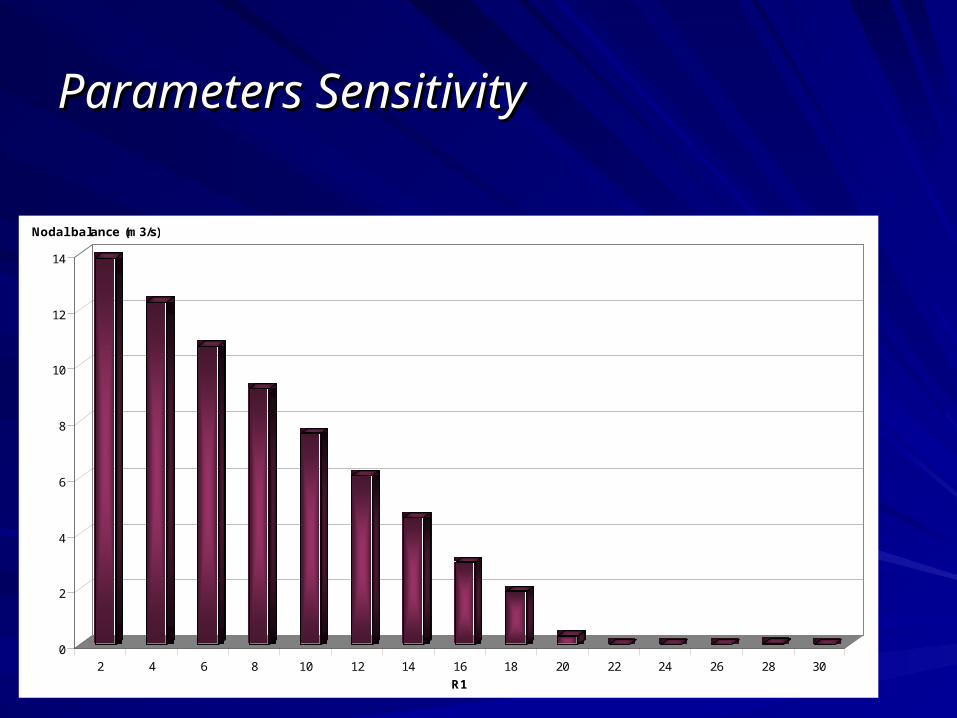
Parameters SensitivityParameters Sensitivity

3.870

3.871

3.872

3.873

3.874

3.875

3.876

3.877

3.878

3.879

3.880

0.000 0.025 0.050 0.075 0.100 0.125 0.150 0.175 0.200 0.225

mutation probability

best fitness

0

10,000

20,000

30,000

40,000

50,000

60,000generation

best fitness

generation

3.80

3.82

3.84

3.86

3.88

3.90

0.4 0.5 0.6 0.7 0.8 0.9 1

crossover probability

best fitness

0

5000

10000

15000

20000

25000

30000

35000

40000

45000

generation

best fitness

generation

Parameters SensitivityParameters Sensitivity

0

2

4

6

8

10

12

14

Nodal balance (m3/s)

2 4 6 8 10 12 14 16 18 20 22 24 26 28 30

R1

Parameters SensitivityParameters Sensitivity

5.10

5.15

5.20

5.25

5.30

5.35

5.40

5.45

5.50

0.0

01

0.0

03

0.0

05

0.0

07

0.0

09

0.0

11

0.0

13

0.0

15

0.0

17

0.0

19

0.0

21

0.0

23

0.0

25

0.0

27

0.0

29

0.0

31

0.0

33

0.0

35

0.0

37

0.0

39

0.0

41

0.0

43

0.0

45

Modified mutation

best fitness

Study resultsStudy results

Drought Drought periodperiod

- GA model give equity in supply in

each canal.

- The ratio of water supply to demand

was nearly equal to 0.6, 0.7, 0.8, and 0.9

in every week.

- WASAM model can not operate in this

period

Study Study resultsresults

0 1 0 2 0 3 02 4 6 8 1 2 1 4 1 6 1 8 2 2 2 4 2 6 2 8 3 2ca n a l n o

0 .0

0 .2

0 .4

0 .6

0 .8

1 .0

sup

ply

/ d

eman

d r

atio

0 1 0 2 0 3 02 4 6 8 1 2 1 4 1 6 1 8 2 2 2 4 2 6 2 8 3 2ca n a l n o

0 .0

0 .2

0 .4

0 .6

0 .8

1 .0

sup

ply

/ d

eman

d r

atio

0 1 0 2 0 3 02 4 6 8 1 2 1 4 1 6 1 8 2 2 2 4 2 6 2 8 3 2ca n a l n o

0 .0

0 .2

0 .4

0 .6

0 .8

1 .0

sup

ply

/ d

eman

d r

atio

F ig u re 4 (co n t): S u p p ly / D eam n d ra tio in ea ch ca n a l (w eek 6 )

su p p ly = 1 .0 * d em a n d

su p p ly = 1 .2 * d em a n d

su p p ly = 1 .5 * d em a n d

Normal and flood Normal and flood periodperiod

- GA model give supply in each canal

not over demand

- Both GA and WASAM give

the similar results

0

5

10

15

20

25

30

35

1 2 3 4 5 6 7 8 9 10 11 12 13 14 15 16 17 18 19 20 21 22 23 24 25 26 27 28 29 30 31 32

คลองส่�งน้ำ�

อ�ตร�ก�รไหลใน้ำคลอง(ม3/วิ�)

GA (sink 0.119 m3/s)

WASAM

Study resultsStudy results

Q (m3/s)

Canal No.