comparison of machine learning models for …
TRANSCRIPT

COMPARISON OF MACHINE LEARNING MODELS FOR
CLASSIFICATION OF BGP ANOMALIES
by
Nabil M. Al-Rousan
B.Sc., Jordan University of Science and Technology, 2009
M.A.Sc., Simon Fraser University, 2012
a Thesis submitted in partial fulfillment
of the requirements for the degree of
Master of Applied Science
in the
School of Engineering Science
Faculty of Applied Sciences
c© Nabil M. Al-Rousan 2012
SIMON FRASER UNIVERSITY
Fall 2012
All rights reserved.
However, in accordance with the Copyright Act of Canada, this work may be
reproduced without authorization under the conditions for “Fair Dealing.”
Therefore, limited reproduction of this work for the purposes of private study,
research, criticism, review and news reporting is likely to be in accordance
with the law, particularly if cited appropriately.

APPROVAL
Name: Nabil M. Al-Rousan
Degree: Master of Applied Science
Title of Thesis: Comparison of Machine Learning Models for Classification of
BGP Anomalies
Examining Committee: Professor Glenn H. Chapman
Chair
Ljiljana Trajkovic
Professor, Engineering Science
Simon Fraser University
Senior Supervisor
Jie Liang
Associate Professor, Engineering Science
Simon Fraser University
Supervisor
William A. Gruver
Professor Emeritus, Engineering Science
Simon Fraser University
SFU Examiner
Date Approved:
ii

Abstract
Worms such as Slammer, Nimda, and Code Red I are anomalies that affect performance of
the global Internet Border Gateway Protocol (BGP). BGP anomalies also include Internet
Protocol (IP) prefix hijacks, miss-configurations, and electrical failures. In this Thesis,
we analyzed the feature selection process to choose the most correlated features for an
anomaly class. We compare the Fisher, minimum redundancy maximum relevance (mRMR),
odds ratio (OR), extended/multi-class/weighted odds ratio (EOR/MOR/WOR), and class
discriminating measure (CDM) feature selection algorithms. We extend the odds ratio
algorithms to use both continuous and discrete features.
We also introduce new classification features and apply Support Vector Machine (SVM)
models, Hidden Markov Models (HMMs), and naive Bayes (NB) models to design anomaly
detection algorithms. We apply multi classification models to correctly classify test datasets
and identify the correct anomaly types. The proposed models are tested with collected BGP
traffic traces from RIPE and BCNET and are employed to successfully classify and detect
various BGP anomalies.
iii
Acknowledgments
This thesis would not have been possible without the support of several thoughtful and
generous individuals. Foremost among those is my advisor Professor Ljiljana Trajkovic
who has provided tremendous insight and guidance on a variety of topics, both within and
outside of the realm of communication networks. I would like to extend my appreciation to
my colleagues in the communication networks laboratory who supported me during writing
of this thesis. Finally, I owe my greatest debt to my family. I thank my parents for life and
the strength and determination to live it. Special thanks to my mother who reminds me
daily that miracles exist everywhere around us.
iv

Contents
Approval ii
Abstract iii
Acknowledgments iv
Contents v
List of Tables vii
List of Figures ix
List of Acronyms xi
1 Introduction 1
1.1 Introduction . . . . . . . . . . . . . . . . . . . . . . . . . . . . . . . . . . . . . 1
1.2 Defining the Problem . . . . . . . . . . . . . . . . . . . . . . . . . . . . . . . . 3
1.3 Purpose of Research . . . . . . . . . . . . . . . . . . . . . . . . . . . . . . . . 4
1.4 Literature Review . . . . . . . . . . . . . . . . . . . . . . . . . . . . . . . . . 4
1.4.1 Statistical techniques . . . . . . . . . . . . . . . . . . . . . . . . . . . . 5
1.4.2 Clustering techniques . . . . . . . . . . . . . . . . . . . . . . . . . . . 5
1.4.3 Rule-based techniques . . . . . . . . . . . . . . . . . . . . . . . . . . . 5
1.4.4 Neural network techniques . . . . . . . . . . . . . . . . . . . . . . . . . 6
1.4.5 Support Vector Machines (SVM) techniques . . . . . . . . . . . . . . . 6
1.4.6 Bayesian networks based approaches . . . . . . . . . . . . . . . . . . . 7
1.5 Research Contributions . . . . . . . . . . . . . . . . . . . . . . . . . . . . . . 7
1.6 Structure of this Thesis . . . . . . . . . . . . . . . . . . . . . . . . . . . . . . 8
v

2 Feature Processing 9
2.1 Extraction of Features . . . . . . . . . . . . . . . . . . . . . . . . . . . . . . . 9
2.2 Selection of Features . . . . . . . . . . . . . . . . . . . . . . . . . . . . . . . . 18
3 Classification 25
3.1 BGP Anomaly Detection . . . . . . . . . . . . . . . . . . . . . . . . . . . . . 25
3.1.1 Definitions . . . . . . . . . . . . . . . . . . . . . . . . . . . . . . . . . 25
3.1.2 Type of Anomalies . . . . . . . . . . . . . . . . . . . . . . . . . . . . . 25
3.1.3 Type of Features . . . . . . . . . . . . . . . . . . . . . . . . . . . . . . 26
3.1.4 Supervised Classification . . . . . . . . . . . . . . . . . . . . . . . . . . 26
3.1.5 Performance Evaluation . . . . . . . . . . . . . . . . . . . . . . . . . . 28
3.2 Classification with Support Vector Machine Models . . . . . . . . . . . . . . . 30
3.2.1 Two-Way Classification . . . . . . . . . . . . . . . . . . . . . . . . . . 33
3.2.2 Four-Way Classification . . . . . . . . . . . . . . . . . . . . . . . . . . 35
3.3 Classification with Hidden Markov Models . . . . . . . . . . . . . . . . . . . . 35
3.4 Classification with naive Bayes Models . . . . . . . . . . . . . . . . . . . . . . 41
3.4.1 Two-Way Classification . . . . . . . . . . . . . . . . . . . . . . . . . . 43
3.4.2 Four-Way Classification . . . . . . . . . . . . . . . . . . . . . . . . . . 45
4 BGPAD Tool 47
5 Analysis of Classification Results and Discussion 56
6 Conclusions 59
References 61
Appendix A Parameter Assumptions 67
vi

List of Tables
2.1 Sample of a BGP update packet. . . . . . . . . . . . . . . . . . . . . . . . . . 10
2.2 Details of BGP datasets. . . . . . . . . . . . . . . . . . . . . . . . . . . . . . . 11
2.3 Extracted features. . . . . . . . . . . . . . . . . . . . . . . . . . . . . . . . . . 12
2.4 Sample of BGP features definition. . . . . . . . . . . . . . . . . . . . . . . . . 14
2.5 Top ten features used for selection algorithms. . . . . . . . . . . . . . . . . . . 20
2.6 List of features extracted for naive Bayes. . . . . . . . . . . . . . . . . . . . . 22
2.7 The top ten selected features F based on the scores calculated by various
feature selection algorithms. . . . . . . . . . . . . . . . . . . . . . . . . . . . . 24
3.1 Confusion matrix. . . . . . . . . . . . . . . . . . . . . . . . . . . . . . . . . . 29
3.2 The SVM training datasets for two-way classifiers. . . . . . . . . . . . . . . . 31
3.3 Performance of the two-way SVM classification. . . . . . . . . . . . . . . . . . 33
3.4 Accuracy of the four-way SVM classification. . . . . . . . . . . . . . . . . . . 35
3.5 Hidden Markov Models: two-way classification. . . . . . . . . . . . . . . . . . 39
3.6 Hidden Markov Models: four-way classification. . . . . . . . . . . . . . . . . . 39
3.7 Accuracy of the two-way HMM classification. . . . . . . . . . . . . . . . . . . 40
3.8 Performance of the two-way HMM classification: regular RIPE dataset. . . . 40
3.9 Performance of the two-way HMM classification: BCNET dataset. . . . . . . 40
3.10 Accuracy of the four-way HMM classification. . . . . . . . . . . . . . . . . . . 41
3.11 The NB training datasets for the two-way classifiers. . . . . . . . . . . . . . . 43
3.12 Performance of the two-way naive Bayes classification. . . . . . . . . . . . . . 44
3.13 Accuracy of the four-way naive Bayes classification. . . . . . . . . . . . . . . . 46
5.1 Comparison of feature categories in two-way SVM classification. . . . . . . . 57
5.2 Performance comparison of anomaly detection models. . . . . . . . . . . . . . 58
vii

A.1 Sample of a BGP update packet. . . . . . . . . . . . . . . . . . . . . . . . . . 67
viii

List of Figures
1.1 The margin between the decision boundary and the closest data points (left).
SVM maximises the margin to a particular choice of decision boundary (right). 7
2.1 Number of BGP announcements in Slammer (top left), Nimda (top right),
Code Red I (bottom left), and regular RIPE (bottom right). . . . . . . . . . . 10
2.2 Samples of extracted BGP features during the Slammer worm attack. Shown
are the samples of (a) number of announcements, (b) number of announce-
ments prefixes, (c) number of withdrawal, (d) number of withdrawals prefixes,
(e) average unique AS-PATH, (f) average AS-PATH, (g) average edit distance
AS-PATH, (h) duplicate announcements, (i) duplicate withdrawal, (j) implicit
withdrawals, (k) inter-arrival time, (l) maximum AS-PATH, (m) maximum
edit distance, (n) number of EGP packets, (o) number of IGP packets, and
(p) number of incomplete packets features. . . . . . . . . . . . . . . . . . . . . 13
2.3 Distributions of the maximum AS-PATH length (left) and the maximum edit
distance (right). . . . . . . . . . . . . . . . . . . . . . . . . . . . . . . . . . . . 15
2.4 Scattered graph of feature 6 vs. feature 1 (left) and vs. feature 2 (right)
extracted from the BCNET traffic. Feature values are normalized to have
zero mean and unit variance. Shown are two traffic classes: regular ({) and
anomaly (∗). . . . . . . . . . . . . . . . . . . . . . . . . . . . . . . . . . . . . 20
2.5 Scattered graph of all features vs. feature 1 (left) and vs. feature 2 (right)
extracted from the BCNET traffic. Feature values are normalized to have
zero mean and unit variance. Shown are two traffic classes: regular ({) and
anomaly (∗). . . . . . . . . . . . . . . . . . . . . . . . . . . . . . . . . . . . . 21
3.1 Supervised classification process. . . . . . . . . . . . . . . . . . . . . . . . . . 27
ix
3.2 4-fold cross-validation process. . . . . . . . . . . . . . . . . . . . . . . . . . . 28
3.3 The SVM classification process. . . . . . . . . . . . . . . . . . . . . . . . . . . 32
3.4 Shown in red is incorrectly classified (anomaly) traffic. . . . . . . . . . . . . . 34
3.5 Shown in red are incorrectly classified regular and anomaly traffic for Slammer
(top left), Nimda (middle left), and Code Red I (bottom left) and correctly
classified anomaly traffic for Slammer (top right), Nimda (middle right), and
Code Red I (bottom right). . . . . . . . . . . . . . . . . . . . . . . . . . . . . 34
3.6 The first order HMM with two processes. . . . . . . . . . . . . . . . . . . . . 36
3.7 The HMM classification process. . . . . . . . . . . . . . . . . . . . . . . . . . 37
3.8 Distribution of the number of BGP announcements (left) and withdrawals
(right) for the Code Red I worm. . . . . . . . . . . . . . . . . . . . . . . . . . 38
3.9 Shown in red are incorrectly classified regular and anomaly traffic for Slammer
(top left), Nimda (middle left), and Code Red I (bottom left); and correctly
classified anomaly traffic for Slammer (top right), Nimda (middle right), and
Code Red I (bottom right) . . . . . . . . . . . . . . . . . . . . . . . . . . . . . 45
4.1 Inspection of BGP PCAPs and MRT files statistics. . . . . . . . . . . . . . . 48
4.2 GUI for two-way SVM models. . . . . . . . . . . . . . . . . . . . . . . . . . . 49
4.3 Two-way SVM graphs. . . . . . . . . . . . . . . . . . . . . . . . . . . . . . . . 50
4.4 GUI for four-way SVM models. . . . . . . . . . . . . . . . . . . . . . . . . . . 51
4.5 GUI for two-way HMM models. . . . . . . . . . . . . . . . . . . . . . . . . . . 52
4.6 GUI for four-way HMM models. . . . . . . . . . . . . . . . . . . . . . . . . . 53
4.7 GUI for two-way NB models. . . . . . . . . . . . . . . . . . . . . . . . . . . . 54
4.8 GUI for four-way NB models. . . . . . . . . . . . . . . . . . . . . . . . . . . . 55
x
List of Acronyms
• AS: Autonomous System
• CIXP: CERN Internet exchange Point
• BGP: Border Gateway Protocol
• BGPAD: Border Gateway Protocol Anomaly Detection Tool
• CDM: Class Discriminating Measure
• DDoS: Distributed Denial of Service
• EGP: Exterior Gateway Protocol
• EOR: Extended Odds Ratio
• HMM: Hidden Markov Model
• IANA: Internet Assigned Numbers Authority
• IETF: Internet Engineering Task Force
• IGP: Interior Gateway Protocol
• IP: Internet Protocol
• ISP: Internet Service Provider
• OR: Odds Ratio
• MRT: Multi-Threaded Routing Toolkit
• MOR: Multiclass Odds Ratio
• mRMR: Minimum Redundancy Maximum Relevance
• NB: Naive Bayes
• NLRI: Network Layer Reachability Information
• RBF: Radial Basis Function
• RIB: Routing Information Base
• thesis: Rseaux IP Europens
• ROC: Receiver Operating Characteristic
• SQL: Structured Query Language
• SVM: Support Vector Machine
• TCP: Transmission Control Protocol
• WOR: Weighted Odds Ratio
xi

Chapter 1
Introduction
1.1 Introduction
Border Gateway Protocol (BGP) routes the Internet traffic [1]. BGP is de facto Inter-
Autonomous System (AS) routing protocol. An AS is a group of BGP peers that are
administrated by a single administrator. The BGP peers are routers that use BGP as
an exterior routing protocol and participate in BGP sessions to exchange BGP messages.
An AS usually relies on an Interior Gateway Protocol (IGP) protocol to route the traffic
within itself [2]. The AS numbers are assigned by the Internet Assigned Numbers Authority
(IANA) [3]. Peer routers exchange four types of messages: open, update, notification, and
keepalive. The main function of BGP is to exchange reachability information among BGP
peers based on a set of metrics: policy decision, the shortest AS-path, and the nearest
next-hop router. BGP operates over a Transmission Control Protocol (TCP) using port
179.
BGP anomalies often occur and techniques for their detection have recently gained
visible attention and importance. Recent research reports describe a number of anomaly
detection techniques. One of the most common approaches is based on a statistical pattern
recognition model that is implemented as an anomaly classifier [4]. Its main disadvantage is
the difficulty in estimating distributions of higher dimensions. Other proposed techniques
are rule-based and require a priori knowledge of network conditions. An example is the
Internet Routing Forensics (IRF) that is applied to classify anomaly events [5]. However,
rule-based techniques are not adaptable learning mechanisms, are slow, and have a high
degree of computational complexity.
1

CHAPTER 1. INTRODUCTION 2
Various anomalies affect Internet servers and hosts and, consequently, slow down the
Internet traffic. Three worms have been considered in this thesis: Slammer, Nimda, and
Code Red I.
The Structured Query Language (SQL) Slammer worm attacked Microsoft SQL servers
on January 25, 2003. The Slammer worm is a code that generates random IP addresses and
replicates itself by sending 376 bytes of code to randomly generated IP addresses. If the
IP address happens to be a Microsoft SQL server or a user PC with Microsoft SQL Server
Data Engine (MSDE) installed, the server becomes infected and begins infecting other
servers [6]. Microsoft released a patch to fix the vulnerability six months before the worm’s
attack. However, the infected servers were never patched. The slowdown of the Internet
traffic was caused by the crashed BGP routers that could not handle the high volume of
the worm traffic. The first flood of BGP update messages was sent to the neighbouring
BGP routers so they could update entries of the crashed routers in the BGP routing tables.
The Slammer worm performed a Denial of Service (DoS) attack. The Internet Service
Provider (ISP) network administrators restarted the routers thus causing a second flood of
BGP update messages. As a result, the update messages consumed most of the routers’
bandwidth, slowed down the routers, and in some cases caused the routers to crash. To
resolve this issue, network administrators blocked port 1434 (the SQL Server Resolution
Service port). Later on, network security companies such as Symantec released patches to
detect the worm payload [7].
The Nimda worm is most known for its very fast spreading. It propagated through the
Internet within 22 minutes. The worm was released on September 18, 2001. It propagated
through email, web browsers, and file systems. In the email propagation, the worm took
the advantage of the vulnerability in the Microsoft Internet Explorer 5.5 SP1 (or earlier
versions) that automatically displayed an attachment included in the email message. The
worm payload is triggered by viewing the email message. In the browsers propagation, the
worm modified the content of the web document file (.htm, .html, or .asp) in the infected
hosts. As a result, the browsed web content, whether it is accessed locally or via a web
server, may download a copy of the worm. In the file system propagation, the worm copies
itself (using the extensions .eml or .nws) in all local host directories including those residing
in the network that the user may access [8].
The Code Red I worm attacked Microsoft Internet Information Services (IIS) web servers
on July 13, 2001. The worm took the advantage of a vulnerability in the indexing software

CHAPTER 1. INTRODUCTION 3
in IIS. By July 19th, the worm affected 359,000 hosts. The worm triggered a buffer overflow
in the infected hosts by writing to the buffers without bounds checking. An infected host
interprets the worms’ message as a computer instruction, which causes the worm to prop-
agate. The worm spreads by generating random IP addresses to get itself replicated and
causes a DoS attack. The worm checks the system’s time. If the date is beyond the 20th of
the month, the worm sends 100 kB of data to port 80 of www.whitehouse.gov. Otherwise,
the worm tries to find new web servers to infect [9]. The worm affected approximately half
a million IP addresses a day.
Variety of behaviours and targets of the described worms increase the importance of
classifying network traffic to detect anomalies [10]. Furthermore, identifying the exact type
of the anomaly helps network administrators protect the company’s data and services.
In this thesis, we employ machine learning techniques to develop models for detecting
BGP anomalies. We extract various BGP features in order to achieve reliable classification
results. We use Support Vector Machine (SVM) models to train and test various datasets.
Hidden Markov Models (HMMs) and naive Bayes (NB) models are also employed to eval-
uate the effectiveness of the extracted traffic features. We then compare the classification
performance of these three algorithms.
1.2 Defining the Problem
Anomaly detection has gained a high importance within the research community and in-
dustry development teams in terms of research projects and developed models. BGP worms
frequently affect the economic growth of the Internet. Many application domains are con-
cerned with anomaly detection. Intrusion, distributed denial of service attacks (DDoS), and
BGP anomaly detections have similar characteristics and use similar detection techniques.
The consensus between researchers and industry on the harmful effects of anomalies is based
on the following properties of the Internet [11]:
• The Internet openness allows attackers to have a cheap, difficult to trace, and easy
way to attack other servers or machines.
• Rapid development of the Internet allows users to devise new ways and tools to attack
and harm other services.

CHAPTER 1. INTRODUCTION 4
• Most Internet traffic is not encrypted, which permits intruders to attack and threaten
the confidentiality and integrity of many web services.
• Due to the rapid growth of the Internet, many applications are designed without taking
into consideration secure ways to access the Internet. This downside makes these
applications vulnerable to frequent attacks and makes the availability of adequate
detection models a crucial factor for the Internet usability.
Technical vulnerabilities that the attackers exploited are software or protocol designs
(Slammer and Code Red I) or system/network configurations (Nimda).
1.3 Purpose of Research
In this thesis, we adapt machine learning algorithms to detect BGP anomalies. The following
issues are addressed:
• We investigate the features and correlations among features in order to identify any
test data point whether a test data point is an anomaly or regular traffic. We develop
a tool to extract 37 BGP features from the BGP traffic. We also explore the effect of
each feature on the classification results. Among the 37 extracted features, we use 21
new features that have not been introduced in the literature.
• We select the best combination of features to achieve the best classification accuracy by
applying and extending some of the existing feature selection algorithms. We compare
the feature selection methods for each classification algorithm and identify the best
features combination for each case.
• We adapt machine learning techniques to classify and detect BGP anomalies. Each
technique has multiple variants that work well for a particular anomaly. We adapt
these variants to maximize the accuracy of detecting the targeted BGP anomalies.
1.4 Literature Review
Many classification techniques have been implemented to detect BGP anomalies. During
the last decade, statistical techniques were dominating classification of BGP anomalies.
Recently, a number of machine learning techniques have been investigated to enhance the

CHAPTER 1. INTRODUCTION 5
performance of anomaly detection techniques [12]. In this Section, we review some well-
known mechanisms for anomaly detection. We group the anomaly detection approaches in
order to compare machine learning techniques used for anomaly detection and evaluate their
advantages and disadvantages.
1.4.1 Statistical techniques
The statistical techniques detect anomalies under the assumption that anomalous traffic oc-
curs with small probability when tested using stochastic models built for regular traffic [13].
Various statistical techniques have been implemented, such as wavelet analysis, covariance
matrix analysis, and principal component analysis. For any statistical techniques, three steps
should be performed: data prepossessing and filtering, statistical analysis, and threshold de-
termination and anomaly detection [12]. The main disadvantage of statistical techniques is
that they assume that the regular traffic is generated from a certain distribution, which is
generally not correct. However, if the assumption of the traffic distribution is valid, their
performance is excellent [14].
1.4.2 Clustering techniques
Clustering belongs to the unsupervised detection techniques. The key principle is to cluster
the regular traffic into one cluster and classify the remaining data points as anomalous
traffic [13]. Clustering groups similar traffic data points into clusters. A strong assumption
of the clustering techniques is that all regular traffic data points belong to one cluster while
anomalous data points may belong to multiple clusters. The main disadvantage of the
clustering techniques is that they are optimized to find the regular traffic rather than the
anomalous traffic that is usually the goal of the detection techniques.
1.4.3 Rule-based techniques
Rule-based techniques build classifiers based on a set of rules. If a test data point is not
matched by any rule, it is classified as an anomaly. A rule-based technique has been im-
plemented [15] where the rules that maximize the classification error were discarded. The
rule-based techniques require a priori knowledge of network conditions. Their main advan-
tage is that they enable multiclass classification. However, the labels for various classes
are not always available. Another advantage is their simplicity that enables them to be

CHAPTER 1. INTRODUCTION 6
visualized as decision trees and interpreted using the classification criteria. For example, if
the number of BGP announcements exceeds certain threshold, it is easy to infer that the
BGP traffic at that time is considered as an anomaly.
1.4.4 Neural network techniques
Many classification models have been implemented using neural networks [16], [17]. A neural
network is a set of neurons that are connected by weighted links that pass signals between
neurons [18]. Neural networks are mathematical models that adapt to the changes in the
layer states by constantly changing structure of the neural model based on the connection
flows in the training stage. Although neural networks have the ability to detect the complex
relationship among features, they have many drawbacks. For example, the high computa-
tional complexity and the high probability of overfitting encouraged researches to use other
classification mechanisms.
1.4.5 Support Vector Machines (SVM) techniques
SVM detects the anomaly patterns in data using nonlinear classification functions. SVM
algorithm classifies each data point based on its value obtained by the classifier function.
SVM builds a classification model that maximizes the margin between the data points
that belong to each class. Figure 1.1 (left) illustrates the margin that SVM maximizes. The
margin is the distance between the SVM classifier (dashed line) and data points (solid lines).
Figure 1.1 (right) illustrates the SVM solution. The maximum margin is the perpendicular
distance between the SVM classifier function (dashed line) and the closest support vectors
(solid lines). The complexity of the SVM model depends on the number of the support
vectors because they control the dimensionality of the classifier function. The complexity of
the SVM model decreases as the numbers of the support vectors decreases. Several variants
of SVM detection techniques are introduced and evaluated [18]. The SVM algorithm has a
high computational complexity because of the quadratic optimization problem that needs
to be solved. However, SVM usually exhibits the best performance in terms of accuracy
and F-score performance indices [19].

CHAPTER 1. INTRODUCTION 7
Class a data pointClass b data pointClassi�er functionMargin
Class a data pointClass b data point
Classi�er functionMargin
Support vector
Figure 1.1: The margin between the decision boundary and the closest data points (left).
SVM maximises the margin to a particular choice of decision boundary (right).
1.4.6 Bayesian networks based approaches
Bayesian approaches are used in many real-time classification systems because of their low
time complexity. Time complexity is a function of input length and measures the execution
time of an algorithm. The Bayesian networks rely on two assumptions: the features are con-
ditionally independent given a target class and the posterior probability is the classification
criteria between any two data point. The posterior probability is calculated based on the
Bayes theorem. Many anomaly detection schemas have implemented variants of Bayesian
networks [20]. The main advantage of Bayesian networks is their low complexity that allows
them to be implemented as online detection systems [21]. Another advantage is that the
testing stage has a constant time computational complexity [22].
1.5 Research Contributions
During the process of investigating the best models for BGP anomaly detection, we address
and solve several issues related to the development of the proposed models. The main
contributions of this thesis are:
• We extract and process BGP traffic data from thesis [23] and BCNET [24] to define
37 BGP features. These features permit us to classify and determine whether a data
point instance is an anomaly.

CHAPTER 1. INTRODUCTION 8
• We investigate the effect of applying feature selection algorithms along with the pro-
posed classifiers. We extend the usage of several algorithms to fit the type of certain
features. For example, we apply the Odds Ratio [25] selection algorithm for both
binary and continuous sets of features. We also discuss a methodology for identifying
the relationship between the category of the features and the classification results.
• We use several machine learning algorithms to classify BGP anomalies. For example,
we use HMM classifiers to classify and detect a sequence of BGP data points. In order
to adapt HMM to detect BGP anomalies, we choose a two-layer, fully connected,
supervised, 10-fold, Balm-Walch trained HMM classifier to detect anomalies in two-
way and four-way classes. We propose efficient models to classify and test sequence of
BGP packets.
• We propose four-way classifiers where the classifier will classify whether the data point
instance is an anomaly and will also classify it into the correct type: Slammer, Nimda,
or Code Red I. This thesis introduces the first multi-classification of BGP anomalies.
• We build a graphical user interface (GUI) tool named BGPAD [26] to classify BGP
anomalies for the extracted BGP datasets and for any user specific datasets. The tool
permits the user to upload a dataset to be tested by the trained models.
1.6 Structure of this Thesis
This thesis is outlined as follows. In Chapter 2, a detailed methodology of features extraction
is proposed. Furthermore, several feature selection algorithms are addressed. In Section 3.1,
the supervised classification process of BGP anomalies is described. Proposed methodologies
based on SVM, HMM, and NB are presented in Sections 3.2, 3.3, and 3.4, respectively. A
user guide for the BGPAD tool is given in Chapter 4. We discuss the results in Chapter 5.
Conclusions are summarized in Chapter 6 along with suggestions for future research.

Chapter 2
Feature Processing
2.1 Extraction of Features
In 2001, Reseaux IP Europeens (RIPE) [23] initiated the Routing Information Service (RIS)
project to collect BGP update messages. Real-time BGP data are also collected by the Route
Views project at the University of Oregon, USA [27]. The RIPE and Route Views BGP
update messages are available to the research community in the multi-threaded routing
toolkit (MRT) binary format [28], which was introduced by the Internet Engineering Task
Force (IETF) to export routing protocol messages, state changes, and contents of the routing
information base (RIB). RIPE and RouteViews projects enlist end-points (routers) to collect
BGP traffic. We collect the BGP update messages that originated from AS 513 (RIPE RIS,
rcc04, CIXP, Geneva) and include a sample of the BGP traffic during time periods when
the Internet experienced BGP anomalies. Various ASes and end-points may be chosen from
RIPE and Route Views to collect the BGP update messages. Due to the global effect of
BGP worms, similar results are obtained. During a worm attack, routing tables of the
entire Internet are affected and, hence, similar traffic trends are observed at different end-
points. We use the Zebra tool [29] to convert MRT to ASCII format and then extract traffic
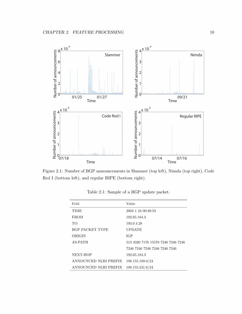
features. Traffic traces of three BGP anomalies along with regular RIPE traffic are shown in
Figure 2.1. A sample of the BGP update message format is shown in Table 2.1. It contains
two Network Layer Reachability Information (NLRI) announcements, which share attributes
such as the AS-PATH. The AS-PATH attribute in the BGP update message indicates the
path that a BGP packet traverses among Autonomous System (AS) peers. The AS-PATH
attribute enables BGP to route packets via the best path.
9
CHAPTER 2. FEATURE PROCESSING 10
01/25 01/270
2
4
6
8x 10
4
Nu
mb
er
of
an
no
un
ce
me
nts
Time
Slammer
09/210
1
2
3
4x 10
4
Nu
mb
er
of
an
no
un
ce
me
nts
Time
Nimda
07/180
1
2
3
4x 10
4
Nu
mb
er
of
an
no
un
ce
me
nts
Time
Code Red I
07/14 07/160
1
2
3
4x 10
4
Nu
mb
er
of
an
no
un
ce
me
nts
Time
Regular RIPE
Figure 2.1: Number of BGP announcements in Slammer (top left), Nimda (top right), Code
Red I (bottom left), and regular RIPE (bottom right).
Table 2.1: Sample of a BGP update packet.
Field Value
TIME 2003 1 24 00:39:53
FROM 192.65.184.3
TO 193.0.4.28
BGP PACKET TYPE UPDATE
ORIGIN IGP
AS-PATH 513 3320 7176 15570 7246 7246 7246
7246 7246 7246 7246 7246 7246
NEXT-HOP 192.65.184.3
ANNOUNCED NLRI PREFIX 198.155.189.0/24
ANNOUNCED NLRI PREFIX 198.155.241.0/24
CHAPTER 2. FEATURE PROCESSING 11
We collect the BGP update messages that originated from:
• RIPE: Routing Information Service (RIS) project
• Autonomous System (AS 513) for European Organization for Nuclear Research Checker
number four
• CERN Internet Exchange Point (CIXP) distributed neutral Internet exchange point
for the Geneva area
• Routing Registry Consistency Check (rcc04) or Routing Configuration.
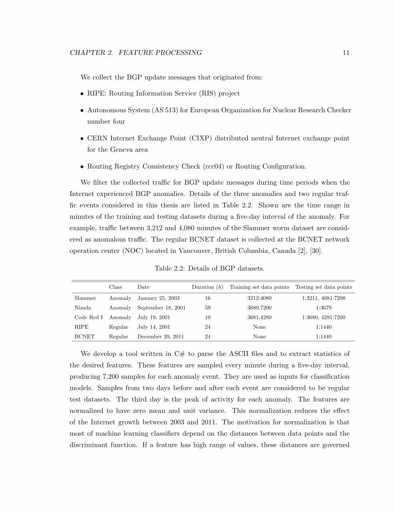
We filter the collected traffic for BGP update messages during time periods when the
Internet experienced BGP anomalies. Details of the three anomalies and two regular traf-
fic events considered in this thesis are listed in Table 2.2. Shown are the time range in
minutes of the training and testing datasets during a five-day interval of the anomaly. For
example, traffic between 3,212 and 4,080 minutes of the Slammer worm dataset are consid-
ered as anomalous traffic. The regular BCNET dataset is collected at the BCNET network
operation center (NOC) located in Vancouver, British Columbia, Canada [2], [30].
Table 2.2: Details of BGP datasets.
Class Date Duration (h) Training set data points Testing set data points
Slammer Anomaly January 25, 2003 16 3212:4080 1:3211, 4081:7200
Nimda Anomaly September 18, 2001 59 3680:7200 1:3679
Code Red I Anomaly July 19, 2001 10 3681:4280 1:3680, 4281:7200
RIPE Regular July 14, 2001 24 None 1:1440
BCNET Regular December 20, 2011 24 None 1:1440
We develop a tool written in C# to parse the ASCII files and to extract statistics of
the desired features. These features are sampled every minute during a five-day interval,
producing 7,200 samples for each anomaly event. They are used as inputs for classification
models. Samples from two days before and after each event are considered to be regular
test datasets. The third day is the peak of activity for each anomaly. The features are
normalized to have zero mean and unit variance. This normalization reduces the effect
of the Internet growth between 2003 and 2011. The motivation for normalization is that
most of machine learning classifiers depend on the distances between data points and the
discriminant function. If a feature has high range of values, these distances are governed
CHAPTER 2. FEATURE PROCESSING 12
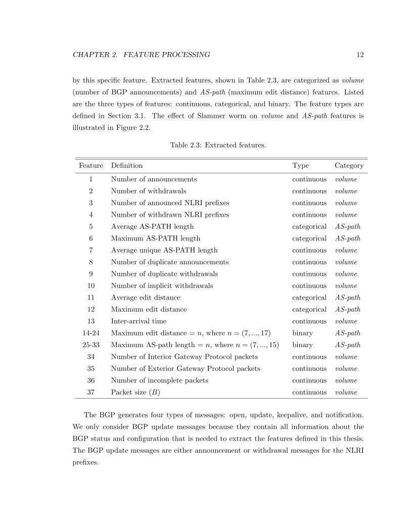
by this specific feature. Extracted features, shown in Table 2.3, are categorized as volume
(number of BGP announcements) and AS-path (maximum edit distance) features. Listed
are the three types of features: continuous, categorical, and binary. The feature types are
defined in Section 3.1. The effect of Slammer worm on volume and AS-path features is
illustrated in Figure 2.2.
Table 2.3: Extracted features.
Feature Definition Type Category
1 Number of announcements continuous volume
2 Number of withdrawals continuous volume
3 Number of announced NLRI prefixes continuous volume
4 Number of withdrawn NLRI prefixes continuous volume
5 Average AS-PATH length categorical AS-path
6 Maximum AS-PATH length categorical AS-path
7 Average unique AS-PATH length continuous volume
8 Number of duplicate announcements continuous volume
9 Number of duplicate withdrawals continuous volume
10 Number of implicit withdrawals continuous volume
11 Average edit distance categorical AS-path
12 Maximum edit distance categorical AS-path
13 Inter-arrival time continuous volume
14-24 Maximum edit distance = n, where n = (7, ..., 17) binary AS-path
25-33 Maximum AS-path length = n, where n = (7, ..., 15) binary AS-path
34 Number of Interior Gateway Protocol packets continuous volume
35 Number of Exterior Gateway Protocol packets continuous volume
36 Number of incomplete packets continuous volume
37 Packet size (B) continuous volume
The BGP generates four types of messages: open, update, keepalive, and notification.
We only consider BGP update messages because they contain all information about the
BGP status and configuration that is needed to extract the features defined in this thesis.
The BGP update messages are either announcement or withdrawal messages for the NLRI
prefixes.

CHAPTER 2. FEATURE PROCESSING 13
03/15 03/16 03/16 03/170
2
4
6x 10
4
Time
An
no
un
cm
en
ts
(a)
01/26 01/270
5
10
15x 10
4
Time
An
no
un
cm
en
ts p
refixe
s(b)
01/26 01/270
5000
10000
15000
Time
With
dra
wa
ls
(c)
01/26 01/270
5
10
15x 10
4
Time
with
dra
wa
ls p
refixe
s
(d)
01/26 01/270
2
4
6
8
Ave
rag
e u
niq
ue
AS
−P
AT
H le
ng
th
Time
(e)
01/26 01/270
2
4
6
8
Ave
rag
e N
um
be
r o
f A
S−
PA
TH
Le
ng
th
Time
(f)
01/25 01/26 01/26 01/270
1
2
3
Ave
rag
e e
dit d
ista
nce
fo
r A
S−
PA
TH
Time
(g)
01/26 01/270
2
4
6x 10
5
Du
plica
te a
nn
ou
nce
me
nts
Time
(h)
01/26 01/270
2
4
6
8x 10
6
Du
plica
te w
ith
dra
wa
ls
Time
(i)
01/26 01/270
0.5
1
1.5
2x 10
6
Imp
licit w
ith
dra
wa
ls
Time
(j)
01/26 01/270
1000
2000
3000
Inte
r a
rriv
al tim
e
Time
(k)
01/26 01/270
10
20
30
Maxim
um
AS
−P
AT
H length
Time
(l)
01/26 01/270
5
10
15
20
Ma
xim
um
ed
it d
ista
nce
Time
(m)
01/26 01/270
20
40
60
80
Nu
mb
er
of
EG
P p
acke
ts
Time
(n)
01/25 01/26 01/26 01/270
1
2
3
4
5x 10
4
Nu
mb
er
of
IGP
pa
cke
ts
Time
(o)
01/26 01/270
1000
2000
3000
4000
Nu
mb
er
of
Inco
mp
lete
pa
cke
ts
Time
(p)
Figure 2.2: Samples of extracted BGP features during the Slammer worm attack. Shownare the samples of (a) number of announcements, (b) number of announcements prefixes, (c)number of withdrawal, (d) number of withdrawals prefixes, (e) average unique AS-PATH,(f) average AS-PATH, (g) average edit distance AS-PATH, (h) duplicate announcements,(i) duplicate withdrawal, (j) implicit withdrawals, (k) inter-arrival time, (l) maximum AS-PATH, (m) maximum edit distance, (n) number of EGP packets, (o) number of IGP packets,and (p) number of incomplete packets features.

CHAPTER 2. FEATURE PROCESSING 14
Feature statistics are computed over one-minute time interval. The NLRI prefixes that
have identical BGP attributes are encapsulated and sent in one BGP packet [31]. Hence,
a BGP packet may contain more than one announced or withdrawal NLRI prefix. While
feature 5 and feature 6 are the average and the maximum number of AS peers in the AS-
PATH BGP attribute, respectively, feature 7 only considers the unique AS-PATH attributes.
Duplicate announcements are the BGP update packets that have identical NLRI prefixes
and AS-PATH attributes. Implicit withdrawals are the BGP announcements with different
AS-PATHs for already announced NLRI prefixes [32]. An example is shown in Table 2.4.
The edit distance between two AS-PATH attributes is the minimum number of insertions,
deletions, or substitutions that need to be executed in order to match the two attributes.
The value of the edit distance feature is extracted by computing the edit distance between
the AS-PATH attributes in each one-minute time interval [4]. For example, the edit distance
between AS-PATH 513 940 and AS-PATH 513 4567 1318 is two because one insertion and
one substitution are sufficient to match the two AS-PATHs. The most frequent values of the
maximum AS-PATH length and the maximum edit distance are used to calculate features
14 to 33. Maximum AS-PATH length and maximum edit distance distributions for the
Slammer worm are shown in Figure 2.3.
Table 2.4: Sample of BGP features definition.
Time Definition BGP update type NLRI AS-PATH
t0 Announcement announcement 199.60.12.130 13455 614
t1 Withdrawal withdrawal 199.60.12.130 13455 614
t2 Duplicate announcement announcement 199.60.12.130 13455 614
t3 Implicit withdrawal announcement 199.60.12.130 16180 614
t4 Duplicate withdrawal withdrawal 199.60.12.130 13455 614
We introduce three new features (34, 35, and 36) shown in Table 2.3, which are based
on distinct values of the ORIGIN attribute that specifies the origin of a BGP update packet
and may assume three values: IGP (generated by an Interior Gateway Protocol), EGP
(generated by the Exterior Gateway Protocol), and incomplete. The EGP is the BGP
predecessor not currently used by the Internet Service Providers (ISPs). However, EGP
packets still appear in traffic traces containing BGP update messages. Under a worm attack,

CHAPTER 2. FEATURE PROCESSING 15
BGP traces contain a large number of EGP packets [32]. The incomplete update messages
imply that the announced NLRI prefixes are generated from unknown sources. They usually
originate from BGP redistribution configurations [31].
0 3 6 9 12 15 18 21 240
200
400
600
Fre
qu
en
cy
Maximum AS PATH length
Slammer
0 2 4 6 8 10 12 14 160
100
200
300
400
Fre
qu
en
cy
Maximum AS PATH edit distnace
Slammer
Figure 2.3: Distributions of the maximum AS-PATH length (left) and the maximum edit
distance (right).Description of the extracted features:
1. Feature 1: The number of BGP update messages with the Type field set to announce-
ment during a one minute interval.
2. Feature 2: The number of BGP update messages with the Type field set to withdrawal
during a one minute interval.
3. Feature 3: The number of announced NLRI prefixes inside BGP update messages with
the Type field set to announcement during a one minute interval.
4. Feature 4: The number of withdrawn NLRI prefixes inside BGP update messages with
the Type field set to withdrawal during a one minute interval.
5. Feature 5: The average length of AS-PATHs of all messages during a one minute
interval.
6. Feature 6: The maximum length of AS-PATHs of all messages during a one minute
interval.
7. Feature 7: The average of unique length of AS-PATHs of all messages during a one
minute interval. The maximum unique AS-PATH is not computed because it is iden-
tical to the maximum AS-PATH.

CHAPTER 2. FEATURE PROCESSING 16
8. Feature 8: The number of duplicate BGP update messages with the Type field set to
announcement during a one minute interval. The message that is counted more than
one time is counted as one duplication.
9. Feature 9: The number of duplicate BGP update messages with the Type field set to
withdrawal during a one minute interval. The message that is duplicated more than
one time is counted as one duplication.
10. Feature 10: The number of BGP update messages during a one minute interval that
have an announcement type and then a withdrawal for the same prefix has been re-
ceived. If another announcement is received after the implicit withdrawal, the message
is considered as a new announcement (feature 1).
11. Feature 11: The average of edit distances among all the messages during a one minute
interval. Listed is the implementation of the edit distance algorithm:
1 Function EditDistance ( [ ] a , [ ] b )
{3 [ , ] EditDistanceArray = new [ a . Length + 1 , b . Length + 1 ]
f o r i = 0 to a . Length
5 EditDistanceArray [ i , 0 ] = i
f o r j = 0 to b . Length
7 EditDistanceArray [ 0 , j ] = j
9 f o r i = 1 to a . Length
{11 f o r j = 1 to b . Length
{13 i f ( a [ i − 1 ] ) = (b [ j − 1 ] )
EditDistanceArray [ i , j ] = EditDistanceArray [ i − 1 , j −1 ]
15 e l s e
EditDistanceArray [ i , j ] = Math .Min(
17 EditDistanceArray [ i − 1 , j ] + 1 ,
Math .Min(
19 EditDistanceArray [ i , j − 1 ] + 1 ,
EditDistanceArray [ i − 1 , j − 1 ] + 1)
21 )
}23 }
r e turn EditDistanceArray [ a . Length , b . Length ]
25 }
27 Function AVG and MAX EditDistnace ( L i s t a )

CHAPTER 2. FEATURE PROCESSING 17
{29 max = 0
min = 1000
31 sum = 0
// break AS−PATH to a l i s t o f s t r i n g s
33 f o r each x in a
{35 AsPathList .Add(x . S p l i t ( ’ ’ ) )
}37
f o r i = 0 to a . Count
39 {f o r j = 0 to i
41 {cur rent = EditDistance ( AsPathList [ i ] , AsPathList [ j ] )
43 sum += current
i f cur r ent > max
45 max = current
i f ( cur r ent < min) and ( i != j ) //Avoid d i s t na c e s with zero
va lue s
47 min = current
}49 }
51 [ ] temp = new [ 3 ]
temp [ 0 ] = max
53 temp [ 1 ] = Math . Ce i l i n g ( ( sum ∗ 1 . 0 ) / ( a . Count ∗ a . Count ) )
temp [ 2 ] = min
55
r e turn temp
57 }
12. Feature 12: The maximum edit distance of all messages during a one minute time
interval.
13. Feature 13: The average inter-arrival time of all messages during a one minute time
interval.
14. Feature 34: The number of BGP update messages that are generated by an Interior
Gateway Protocol (IGP) such as OSPF.
15. Feature 35: The number of BGP update messages that are generated by EGP, which
is the BGP predecessor. Since the value of the BGP update message type is one of

CHAPTER 2. FEATURE PROCESSING 18
the BGP policies, network administrators may configure the attribute value so that
they may reroute the BGP packets based on BGP policies.
16. Feature 36: The incomplete update messages imply that the announced NLRI prefixes
are generated from unknown sources. They usually originate from BGP redistribution
configurations [31].
17. Feature 37: The average of all BGP update messages in bytes.
2.2 Selection of Features
To highlight the importance of feature selection algorithms, we first define dimensionality
as the number of features for each data sample. As shown in Table 2.3, 37 features are
extracted. High dimensionality of the design matrix is considered undesirable because it
increases the computational complexity and memory usage [11]. It also leads to poor
classification results. To reduce the dimensionality, a subset of the original set of features
should be selected or a transformation of a subset of features to new features is needed.
Hence, before applying machine learning algorithms, we address the dimensionality of the
design matrix and try to reduce the number of extracted features. We use the Fisher [34], [35]
and minimum Redundancy Maximum Relevance (mRMR) [36] feature selection algorithms
to select the most relevant features. These algorithms measure the correlation and relevancy
among features and, hence, help improve the classification accuracy. We select the top ten
features for the Fisher feature selection and, thus, neglect the weak and distorted features
in the classification models [4].
Each training datasets is represented as a real matrix X7200×37. Each column vector
Xk, k = 1, ..., 37, corresponds to one feature. The Fisher score for Xk is computed as:
Fisher score =m2
a −m2r
s2a + s2r
ma =1
Na
∑i∈anomaly
xik
mr =1
Nr
∑i∈regular
xik

CHAPTER 2. FEATURE PROCESSING 19
s2a =1
Na
∑i∈anomaly
(xik −ma)2
s2r =1
Nr
∑i∈regular
(xik −mr)2, (2.1)
where Na and Nr are the number of anomaly and regular data points, respectively; and ma
and s2a (mr and s2r) are the mean and the variance for the anomaly (regular) class, respec-
tively. The Fisher algorithm maximizes the inter-class separation m2a −m2
r and minimizes
the intra-class variances s2a and s2r .
The mRMR algorithm minimizes the redundancy among features while maximizing
the relevance of features with respect to the target class. We use three variants of the
mRMR algorithm: Mutual Information Difference (MID), Mutual Information Quotient
(MIQ), and Mutual Information Base (MIBASE). The mRMR relevance of a feature set
S = {X1, ...,Xk,Xl, ...,X37} for a class vector Y is based on the mutual information func-
tion I:
I(Xk,Xl) =∑k,l
p(Xk,Xl)logp(Xk,Xl)
p(Xk)p(Xl). (2.2)
The mRMR variants are defined by the criteria:
MID: max [V (I)−W (I)]
MIQ: max [V (I)/W (I)], (2.3)
where:
V (I) =1
|S|∑Xk∈S
I(Xk,Y)
W (I) =1
|S|2∑
Xk,Xl∈SI(Xk,Xl)
and constant |S| is the length of the set S. The MIBASE feature scores are ordered based
on their values (2.2). The Fisher and mRMR scores are obtained for a set of features of
arbitrary captured BGP messages during a one-day interval on January 25, 2003. The set
contains 1,440 samples, where 869 samples are labeled as anomalies. The top ten features
using the Fisher and mRMR algorithms are listed in Table 2.5. They are evaluated in
Section 3.2 by using the SVM classification.

CHAPTER 2. FEATURE PROCESSING 20
Table 2.5: Top ten features used for selection algorithms.
mRMR
Fisher MID MIQ MIBASE
Feature Score Feature Score Feature Score Feature Score
11 0.39 34 0.94 34 0.94 34 0.94
6 0.35 32 0.02 2 0.33 36 0.63
25 0.29 33 0.02 8 0.34 2 0.47
9 0.27 2 0.01 24 0.31 8 0.34
2 0.18 31 0.02 9 0.33 9 0.27
36 0.12 24 0.01 14 0.30 3 0.13
37 0.12 8 0.01 1 0.35 1 0.13
24 0.12 14 0.02 36 0.36 6 0.10
8 0.11 30 0.02 3 0.30 12 0.08
14 0.08 22 0.02 25 0.27 11 0.06
The scatterings of anomalous and regular classes for feature 6 (AS-path) vs. feature 1
(volume) and feature 6 (AS-path) vs. feature 2 (volume) in two-way classifications are shown
in Figure 2.4 (left) and Figure 2.4 (right), respectively. The graphs indicate spatial separa-
tion of features. While selecting feature 1 and feature 6 may lead to a feasible classification
based on visible clusters ({and ∗), using only feature 2 and feature 6 would lead to poor
classification. Hence, selecting an appropriate combination of features is essential for an
accurate classification. The scatterings of anomalous and regular classes for all features vs.
feature 1 (volume) and vs. feature 2 (volume) are shown in Figure 2.5.
−4 −2 0 2 4 6−2
0
2
4
6
8
Feature 1
Fe
atu
re 6
Regular
AnomalyBCNET
−4 −2 0 2 4 6−2
0
2
4
6
8
Feature 2
Fe
atu
re 6
Regular
AnomalyBCNET
Figure 2.4: Scattered graph of feature 6 vs. feature 1 (left) and vs. feature 2 (right)
extracted from the BCNET traffic. Feature values are normalized to have zero mean and
unit variance. Shown are two traffic classes: regular ({) and anomaly (∗).

CHAPTER
2.FEATURE
PROCESSIN
G21
Feature 1 Feature 2
17
16
15
14
13
12
11
10
98
76
54
3 −1
1
Figure 2.5: Scattered graph of all features vs. feature 1 (left) and vs. feature 2 (right) extracted from the BCNET traffic.
Feature values are normalized to have zero mean and unit variance. Shown are two traffic classes: regular ({) and anomaly
(∗).

CHAPTER 2. FEATURE PROCESSING 22
Performance of anomaly classifiers depends on the feature selection algorithms [33]. We
calculate the top ten features listed in Table 2.5 to be used in SVM, HMM, and NB classifiers.
In case of SVM, we use the top ten features from each method listed in Table 2.5 as input
for each classifier. In case of HMM, we arbitrarily select four features from the top ten
features (two volume features and two AS-path) features to investigate the effect of feature
categories on the detection performance. These four features are mapped to sequences and
are then used as input to HMM classifiers. Other features could have been also used. For
NB classification, we ignore binary features 14 through 33 because we use continuous and
categorical features. The combination of the continuous and categorical features shows
better performance than the combination of all feature types. We illustrate the difference
among continuous, categorical, and binary features in Section 3.1. The extracted features
for NB are listed in Table 2.6. The extracted features are considered as a feature design
matrix for NB models in Section 3.4. We apply the same top ten features shown in Table 2.5.
We also introduce a set of features selection algorithms that work well only with Bayesian
classifiers. The applied algorithms are: odds ratio (OR), extended/multiclass/weighted odds
ratio (EOR/MOR/WOR), and the class discriminating measure (CDM) [25].
Table 2.6: List of features extracted for naive Bayes.
Feature (F) Definition Category
1 Number of announcements volume2 Number of withdrawals volume3 Number of announced NLRI prefixes volume4 Number of withdrawn NLRI prefixes volume5 Average AS-PATH length AS-path6 Maximum AS-PATH length AS-path7 Average unique AS-PATH length AS-path8 Number of duplicate announcements volume9 Number of duplicate withdrawals volume10 Number of implicit withdrawals volume11 Average edit distance AS-path12 Maximum edit distance AS-path13 Inter-arrival time volume14 Number of Interior Gateway Protocol packets volume15 Number of Exterior Gateway Protocol packets volume16 Number of incomplete packets volume17 Packet size volume

CHAPTER 2. FEATURE PROCESSING 23
The OR algorithm and its variants perform well for selecting features to be used in
binary classification with NB models. In binary classification with two target classes c and
c, the odds ratio of feature Xk is calculated as:
OR(Xk) = logPr(Xk|c)
(1− Pr(Xk|c)
)Pr(Xk|c)
(1− Pr(Xk|c)
) , (2.4)
where Pr(Xk|c) and Pr(Xk|c) are the probabilities of feature Xk being in classes c and c,
respectively.
The EOR, WOR, MOR, and CDM are variants that enable multiclass feature selection.
In case of a classification problem with γ = {c1, c2, . . . , cJ} classes:
EOR(Xk) =J∑
j=1
logPr(Xk|cj)
(1− Pr(Xk|cj)
)Pr(Xk|cj)
(1− Pr(Xk|cj)
)WOR(Xk) =
J∑j=1
Pr(cj)× logPr(Xk|cj)
(1− Pr(Xk|cj)
)Pr(Xk|cj)
(1− Pr(Xk|cj)
)
MOR(Xk) =J∑
j=1
∣∣∣∣∣ logPr(Xk|cj)
(1− Pr(Xk|cj)
)Pr(Xk|cj)
(1− Pr(Xk|cj)
)∣∣∣∣∣CDM(Xk) =
J∑j=1
∣∣∣∣∣ logPr(Xk|cj)Pr(Xk|cj)
∣∣∣∣∣, (2.5)
where Pr(Xk|cj) is the conditional probability of Xk given the class cj and Pr(cj) is the
probability of occurrence of the jth class. The OR algorithm may be extended by computing
Pr(Xk|cj) for continuous features. If the sample points are independent and identically
distributed, (2.4) may be written as:
OR(Xk) =
|Xk|∑i=1
logPr(Xik = xik|c)
(1− Pr(Xik = xik|c)
)Pr(Xik = xik|c)
(1− Pr(Xik = xik|c)
) ,where |Xk| and Xik denote the size and the ith element of the kth feature vector, respectively.
A realization of the random variable Xik is denoted by xik. Other variants of the OR
algorithm may be extended to continuous cases in a similar manner. The top ten selected
features are listed in Table 2.7.

CHAPTER
2.FEATURE
PROCESSIN
G24
Table 2.7: The top ten selected features F based on the scores calculated by various feature selection algorithms.
Fisher mRMR Odds Ratio variants
MID MIQ MIBASE OR EOR WOR MOR CMD
F Score F Score F Score F Score F Score F Score F Score F Score F Score
11 0.397758 15 0.94 15 0.94 15 0.94 10 1.3602 5 2.1645 5 1.3963 6 2.3588 5 8.5959
6 0.354740 5 0.12 12 0.36 17 0.63 4 1.3085 7 2.1512 7 1.3762 5 2.3486 11 6.9743
9 0.271961 12 0.11 3 0.35 2 0.47 1 1.1088 6 2.1438 6 1.3648 11 2.3465 9 3.0844
2 0.185844 7 0.10 8 0.34 8 0.34 14 1.1080 11 2.1340 11 1.3495 17 2.3350 2 2.3485
16 0.123742 4 0.07 1 0.32 6 0.27 12 1.0973 10 2.0954 13 1.1963 16 2.3247 8 2.2402
17 0.121633 10 0.07 6 0.30 3 0.13 3 1.0797 4 2.0954 9 1.0921 14 2.1228 16 2.0985
8 0.116092 8 0.04 4 0.27 1 0.13 15 1.0465 13 2.0502 2 1.0198 1 2.1109 3 2.0606
3 0.086124 13 0.04 17 0.26 9 0.10 8 1.0342 9 2.0127 16 0.9850 2 2.1017 14 2.0506
1 0.081760 2 0.03 9 0.25 12 0.08 17 1.0304 1 2.0107 17 0.9778 7 2.0968 1 2.0417
14 0.081751 14 0.03 2 0.24 11 0.06 16 1.0202 14 2.0105 8 0.9751 3 2.0897 17 2.0213

Chapter 3
Classification
3.1 BGP Anomaly Detection
3.1.1 Definitions
BGP anomalies are the BGP packets that exhibit unusual patterns. They are also referred to
as outliers. The BGP anomaly detection classifier is a machine learning model that learns
how to change its internal structure based on external feedback [38]. Machine learning
models learn to classify data points using a feature matrix. The matrix rows correspond to
data points while the columns correspond to the feature values. A feature is a measurable
property of the system that may be observed. Even though machine learning may provide
general models to classify anomalies, it may easily misclassify test data points. By providing
a sufficient and related set of features, machine learning models may overcome this deficiency
and may help built a generalized model to classify data with the least error rate.
3.1.2 Type of Anomalies
Anomaly detection techniques consider these three types of anomalies:
• Point anomalies: If each data point of the training dataset may be considered as
anomaly.
• Contextual anomalies: The term contextual anomaly [40] refers to an anomaly as the
behaviour of a data instance in a specific context. For example, a large number of
BGP packets may be considered as regular traffic during the peak activity hours of
25

CHAPTER 3. CLASSIFICATION 26
the working days. However, the same pattern may be classified as an anomaly in the
off-peak hours.
• Collective anomalies: A sequence of data points is considered anomalous relative to
the entire set. One data point may be considered as regular traffic. However, it is
considered as anomaly with a collection of neighbouring data points. This type of
anomaly is the most difficult to capture because the classifier should recognize the
temporal relationship among the data points [42].
BGP anomalies in this thesis are treated as point anomalies. The BGP packets are
grouped for each one minute interval. Each training data point may be classified as anomaly
or regular class.
3.1.3 Type of Features
The type of the features determines the applicable classification technique. For example,
the NB classifier works very well with categorical features while statistical models work well
with continuous and categorical features. The features represented in this thesis belong to
three types:
• Binary: Feature may have two values.
• Categorical: Feature may have finite number of values.
• Continuous: Feature may have infinite number of values. Sampling techniques dis-
cretize the continuous features into the categorical type.
The proposed BGP features listed in Table 2.3 belong to all the three types.
3.1.4 Supervised Classification
Supervised classification is one aspect of learning that has supervised (observed) measure-
ments that are labeled with a pre-defined class. During the test stage, the data points
are classified as one of the predefined classes. In unsupervised classification, the task is to
establish the existence of classes or clusters in the training data. Classification is one of the
machine learning categories. Other categories include regression and reinforcement. Learn-
ing implies that given a training dataset, a task is performed after learning the system’s
performance. The performance is measured by a performance index. The efficiency of the

CHAPTER 3. CLASSIFICATION 27
proposed machine learning models is discussed in Section 3.1.5. The task in classification is
to categorize the test labels into pre-defined classes. We define two-way and four-way clas-
sifications. In the two-way classification, two classes are defined: anomalous and regular.
In the four-way classification, four classes are defined: Slammer, Nimda, Code Red I, and
Regular. General steps of a classification process are shown in Figure 3.1. In the training
stage, the training set consists of the sample data points and the associated labels. A sample
data point consists of a set of predefined features. Next, the training dataset is fed into a
machine learning model to build a classifier model that is used later to examine the test
datasets. The classifier model is the criteria set by a machine learning model. In the testing
stage, a testing dataset is processed to extract the design matrix. Next, a classifier model is
applied to the design matrix to generate labels. The last step in the supervised classification
process is to compare this generated set of labels from the testing step with the training set
of labels to evaluate the performance of the model. For example, if the training datasets
are the collected BGP update messages, the task is to classify each data point to anomaly
or regular and the performance measure is F-score (3.5).
Feature
extraction
Machine
learning
algorithm
Feature
extraction
Classifier
modelLabels
Training
dataset
Testing
dataset
Features
Features
Labels
Training
Testing
Figure 3.1: Supervised classification process.
In the training stage, a common procedure named cross-validation is usually performed

CHAPTER 3. CLASSIFICATION 28
to remedy the drawback of overfitting the classifier function. Overfitting phenomenon im-
plies the fact that the testing classification accuracy may not be as good as the training
accuracy. Overfitting is undesired behaviour in machine learning and it is usually caused
by rather complex trained models. For example, in curve fitting problems, if a 9th degree
polynomial is used to fit 3 points, then it is highly probable that poor fitting will result in
the testing stage because test data points will be scattered on a linear, 2nd, or 3rd polyno-
mial function while the fitting polynomial function has a the degree 9. A cross-validation
process is usually used to reduce the overfitting effect. The concept of cross-validation is
to choose the best parameters of the machine learning model parameters that reduce the
training error. A 4-fold cross-validation process is shown in Figure 3.2. To choose the best
value of a parameter, four runs are needed to cover the case of using each fold as a testing
set and the other three as training sets.
Figure 3.2: 4-fold cross-validation process.
The training dataset portion should be larger than the test dataset in order to capture
the anomalous trends. In 2-fold cross-validation, the training dataset portion is equal to
the testing dataset. A 10-fold cross-validation is commonly used as a compromise [39].
Parameters used in this thesis are given in Appendix A.
3.1.5 Performance Evaluation
We measure the performance of the models based on statistical indices. We consider ac-
curacy, balanced accuracy, and F-score as performance indices to compare the proposed
models. They are calculated based on the following definitions:
• True positive (TP): The number of anomalous training data points that are classified
as anomaly.
• True negative (TN): The number of regular training data points that are classified as
regular.

CHAPTER 3. CLASSIFICATION 29
• False positive (FP): The number of regular training data points that are classified as
anomaly.
• False negative (FN): The number of anomalous training data points that are classified
as regular.
These definitions are shown in Table 3.1.
Table 3.1: Confusion matrix.
Actual class
True (anomaly) False (regular)
Anomaly test outcomePositive TP FP
Negative FN TN
We aim to classify a single class (anomaly), which usually has a smaller portion of
the training dataset. Hence, we aim to find the proper performance indices that reflect the
accuracy and precision of the classifier for anomaly training data points. These performance
measures are calculated as:
sensitivity =TP
TP + FN
(3.1)
precision =TP
TP + FP.
(3.2)
The performance indices are calculated as:
accuracy =TP + TN
TP + TN + FP + FN
(3.3)
balanced accuracy =sensitivity + precision
2.
(3.4)
Sensitivity, also known as recall, measures the ability of the model to identify the anomalies
(TP) among all labeled anomalies (true). Precision is the ability of the model to identify the

CHAPTER 3. CLASSIFICATION 30
anomalies (TP) among all data points that are identified as anomalous (positive). Speci-
ficity reflects the ability of the model to identify the regular traffic (true negative) among
all regular traffic (false). Accuracy treats the regular data points as important as anoma-
lous training data. Hence, it is not a good measure to compare performance of classifiers
performance. For example, if a dataset contains 900 regular and 100 anomalous data points
and the NB model classifies the 1,000 training data points as regular, then the accuracy is
90%. At the first glance, this accuracy seems high. However, no anomalous data point is
correctly classified. F-score is often used as a performance index to compare performance
of classification models. It is the harmonic mean of the sensitivity and the precision:
F-score = 2× precision× sensitivityprecision+ sensitivity
.
(3.5)
The harmonic mean tends to be closer to the smaller of the two. Hence, to obtain a large
score value, both precision and sensitivity should be large.
The balanced accuracy is an alternative performance index that is equal to the aver-
age of sensitivity and specificity. F-score reflects the success of detecting anomalies rather
than detecting both anomalies and regular data points. While accuracy and balanced accu-
racy give equal importance to the regular and the anomaly traffic, F-score emphasizes the
anomaly classification rate. Hence, we used F-score to measure the performance of SVM,
HMM, and NB models.
3.2 Classification with Support Vector Machine Models
Support vector machines were introduced by V. Vapnik in the 1970s [41]. SVMs are linear
classifiers that find a hyperplane to separate two classes of data: positive and negative. SVM
are extended for non linear separation using kernels. In real world classification problems,
SVM performs more accurately than most other machine learning models, especially for
datasets with very high dimensional complexity.
We use the SVM classification as a supervised deterministic model to classify BGP
anomalies. MATLAB libsvm-3.1 toolbox [43] is used to train and test the SVM classifiers.
The dimensions of the feature matrix is 7, 200×10, which corresponds to a five-day interval.
Each matrix row corresponds to the top ten selected features during the one-minute interval.

CHAPTER 3. CLASSIFICATION 31
For each training dataset X7200×37, we target two classes: anomaly (true) and regular (false).
The SVM algorithms solves an optimization problem [44] with the constraints:
minCM∑
m=1
ξm +1
2‖w‖2
tmy(Xm) ≥ 1− ξm. (3.6)
Constant C > 0 controls the importance of the margin while slack variable ξm solves the
non-separable data points classification problem. A regularization parameter 12‖w‖
2 is used
to avoid the overfitting. SVM classifies each data point Xm with a training target class
tm either as anomaly y = 1 or regular traffic y equal −1. Xm corresponds to a row vector
where m = 1, ..., 7200. The SVM solution maximizes the margin between the data points
and the decision boundary. Data points that are closest to the decision boundary are called
support vectors. The Radial Basis Function (RBF) kernel is used to avoid the using of the
feature matrix of high dimension by mapping the feature space into a linear space:
K(Xk,Xl) = exp(−γ ∗ ‖Xk −Xl‖2). (3.7)
The RBF kernel K depends on the Euclidean distance between Xk and Xl features [45].
Constant γ influences the number of support vectors. The datasets are trained using 10-fold
cross validation to select parameters (C, γ) that provide the best accuracy. We apply SVM
on sets listed in Table 3.2 to classify BGP anomalies. The SVM classification process is
shown in Figure 3.3.
First, a batch of BGP update messages is processed to generate the feature matrix as
discussed in Chapter 2. Next, the training process takes the design matrix as an input
and cross-validates C and γ to generate the best classifier model. In the testing stage, the
classifier model is used to evaluate the testing datasets and to generate its labels that are
later used to calculate the performance indices.
Table 3.2: The SVM training datasets for two-way classifiers.
NB Training dataset Test dataset
SVM1 Slammer and Nimda Code Red ISVM2 Slammer and Code Red I NimdaSVM3 Nimda and Code Red I Slammer

CHAPTER 3. CLASSIFICATION 32
Figure 3.3: The SVM classification process.

CHAPTER 3. CLASSIFICATION 33
3.2.1 Two-Way Classification
In a two-way classification, all anomalies are treated as one class. Their performance is
shown in Table 3.3. SVM3 model achieves the best F-score (86.1%) using features selected
by the MIQ feature selection algorithm. We check the validity of the proposed models by
applying the two-way SVM classification on the BGP traffic trace that was collected from
the BCNET [24] on December 20, 2011. All data points in the BCNET traffic trace are
labeled as regular traffic. Hence, parameter y = −1. The classification accuracy of 79.2%
indicates the number of data points that are classified as regular traffic. The best two-way
classification result is achieved by using SVM2. Since all data points in BCNET and RIPE
test datasets contain no anomalies, they have low sensitivities and, hence, low F-scores.
Therefore, we calculate instead accuracy as the performance measure. Data points that are
classified as anomalies (false positive) are shown in Figure 3.4.
Table 3.3: Performance of the two-way SVM classification.
Performance index
Accuracy (%) F-score (%)
SVM Feature Test
dataset
(anomaly)
RIPE
(regular)
BCNET
(regular)
Test
dataset
(anomaly)
SVM1 All features 64.1 55.0 62.0 63.2
SVM1 Fisher 72.6 63.2 58.5 73.4
SVM1 MID 63.1 52.2 59.4 61.2
SVM1 MIQ 60.7 47.9 61.7 57.8
SVM1 MIBASE 79.1 74.3 60.9 80.1
SVM2 All features 68.6 97.7 79.2 22.2
SVM2 Fisher 67.4 96.6 74.8 16.3
SVM2 MID 67.9 97.4 72.5 19.3
SVM2 MIQ 67.7 97.5 76.2 15.3
SVM2 MIBASE 67.5 96.8 78.8 17.8
SVM3 All features 81.5 92.0 69.2 84.6
SVM3 Fisher 89.3 93.8 68.4 75.2
SVM3 MID 75.4 92.8 71.7 79.2
SVM3 MIQ 85.1 92.2 73.2 86.1
SVM3 MIBASE 89.3 89.7 69.7 80.1

CHAPTER 3. CLASSIFICATION 34
Test data points from various worms that are incorrectly classified in the two-way classi-
fication (false positives and false negatives) are shown in Figure 3.5 (left column). Correctly
classified as anomalies (true positives) are shown in Figure 3.5 (right column).
12:00AM 12:00PM 12:00AM0
20
40
60
80
100
120
Time
Nu
mb
er
of
IGP
pa
cke
ts
Figure 3.4: Shown in red is incorrectly classified (anomaly) traffic.
01/25 01/270
1
2
3
4
x 104
Time
Nu
mb
er
of
IGP
pa
cke
ts Slammer
Red: FP and FN
Blue: TP and TN
01/25 01/270
1
2
3
4
x 104
Time
Nu
mb
er
of
IGP
pa
cke
ts
Slammer
Red: TP
Blue: TN, FN, and FP
09/20 09/220
0.5
1
1.5
2
x 104
Time
Nu
mb
er
of
IGP
pa
cke
ts
Nimda
Red: FP and FN
Blue: TP and TN
09/20 09/220
0.5
1
1.5
2
x 104
Time
Nu
mb
er
of
IGP
pa
cke
ts
Nimda
Red: TP
Blue: TN, FN, and FP
07/230
0.5
1
1.5
2x 10
4
Time
Nu
mb
er
of
IGP
pa
cke
ts
Code Red I
Red: TP
Blue: TN, FN, and FP
Figure 3.5: Shown in red are incorrectly classified regular and anomaly traffic for Slammer
(top left), Nimda (middle left), and Code Red I (bottom left) and correctly classified anomaly
traffic for Slammer (top right), Nimda (middle right), and Code Red I (bottom right).

CHAPTER 3. CLASSIFICATION 35
3.2.2 Four-Way Classification
We extend the proposed classifier to implement multiclass SVMs and used one-versus-one
multiclass classification [46] on four training datasets: Slammer, Nimda, Code Red I, and
RIPE. A multiclass classification combines a number of two-class classifications. To cover
all classification combinations, data points are classified by n(n− 1)/2 classifiers, where n
is the number of classes. Each data point is classified according to the maximum value
of the classifier function [44]. The four-way classification detects and classifies the specific
type of traffic: Slammer, Nimda, Code Red I, or Regular. Classification performance is
shown in Table 3.4. The BCNET dataset is also tested using the multiclass SVM. The
average accuracy achieved by using BCNET dataset is 91.4%. This is an example of how
the proposed multiclass models perform a recently collected BGP datasets. It shows that
the proposed model has 91.4% probability to classify data points to the correct class type.
The miss-classified data points show that the proposed model may be improved. Possible
solutions are discussed in Chapter 5.
Table 3.4: Accuracy of the four-way SVM classification.
Average accuracy (%)
(3 anomalies concatenated with 1 regular)
Feature RIPE BCNET
All features 77.1 91.4
Fisher 82.8 85.7
MID 67.8 78.7
MIQ 71.3 89.1
MIBASE 72.8 90.2
3.3 Classification with Hidden Markov Models
The second model for classification is based on the first order Hidden Markov Models
(HMMs). HMMs are statistical tools that are used to model stochastic processes that consist
of two embedded processes: the observable process that maps BGP features and the unob-
served hidden process that has the Markovian property. We assume that the observations
are independent and identically distributed. Even though HMMs belong to non-parametric

CHAPTER 3. CLASSIFICATION 36
supervised classification methods, we use 10-fold cross validation to select number of hidden
states as a parameter in order to improve the accuracy of the model. We implement the
HMMs using the MATLAB statistical toolbox. A first order HMM processes is shown in
Figure 3.6. Each HMM model is specified by a tuple λ = (N,M,α, β, π), where:
States
Observations
Figure 3.6: The first order HMM with two processes.
N = number of hidden states (cross-validated)
M = number of observations (11)
α = transition probability distribution N ×N matrix
β = emission probability distribution N ×M matrix
π = initial state probability distribution matrix.
The proposed detection model consists of three stages:
• Sequence extractor and mapping: All features are mapped to 1-D observation vector.
• Training: Two HMMs for two-way classification and four HMMs for four-way classifi-
cation are trained to identify the best α and β for each class. HMMs are trained and
validated for various number of hidden states N .
• Classification: The maximum likelihood probability p(x|λ) is used to classify the test
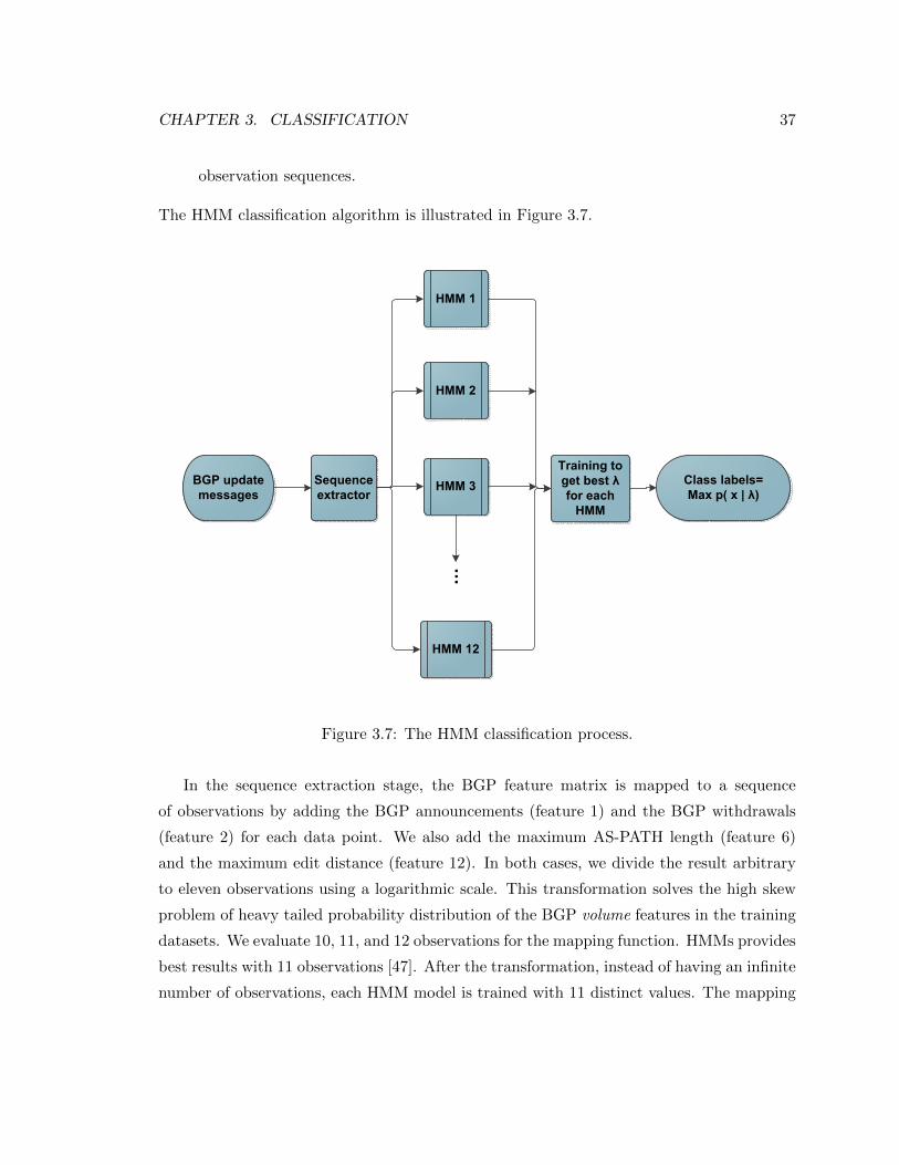
CHAPTER 3. CLASSIFICATION 37
observation sequences.
The HMM classification algorithm is illustrated in Figure 3.7.
Sequence
extractor
HMM 1
HMM 2
HMM 12
Training to
get best λ
for each
HMM
BGP update
messages
Class labels=
Max p( x | λ)HMM 3
...
Figure 3.7: The HMM classification process.
In the sequence extraction stage, the BGP feature matrix is mapped to a sequence
of observations by adding the BGP announcements (feature 1) and the BGP withdrawals
(feature 2) for each data point. We also add the maximum AS-PATH length (feature 6)
and the maximum edit distance (feature 12). In both cases, we divide the result arbitrary
to eleven observations using a logarithmic scale. This transformation solves the high skew
problem of heavy tailed probability distribution of the BGP volume features in the training
datasets. We evaluate 10, 11, and 12 observations for the mapping function. HMMs provides
best results with 11 observations [47]. After the transformation, instead of having an infinite
number of observations, each HMM model is trained with 11 distinct values. The mapping

CHAPTER 3. CLASSIFICATION 38
function for features Xk and Xl is:
log(Xk +Xl)
11. (3.8)
The distribution for BGP announcements during the Code Red I worm attack is shown in
Figure 3.8.
0 500 1000 15000
100
200
300
400
Fre
qu
en
cy
Number of announcments
Code Red I
0 50 100 1500
50
100
150
200
Fre
qu
en
cyNumber of withdrawals
Code Red I
Figure 3.8: Distribution of the number of BGP announcements (left) and withdrawals (right)
for the Code Red I worm.
HMMs are trained and validated for a various number of hidden states. A 10-fold cross-
validation with the Balm-Welch algorithm [44] is used for training to find the best α and
β for each HMM. The best transition and emission matrices are validated by obtaining
the largest maximum likelihood probability p(x|λHMMx). We construct 6 and 12 HMM
models for two-way and four-way classifications, respectively. Various HMMs are listed in
Table 3.5 and Table 3.6. We evaluate the test observation sequences and calculate maximum
likelihood probability for each HMM.
In the classification stage, each test observation sequence is classified based on the largest
maximum likelihood probability for HMMs with the same number of hidden states. For
example, HMM1, HMM4, HMM7, and HMM10 shown in Table 3.6 correspond to HMMs
with two hidden states for various training datasets.

CHAPTER 3. CLASSIFICATION 39
Table 3.5: Hidden Markov Models: two-way classification.
Number of hidden states
Training dataset 2 4 6
Slammer, Nimda, and Code Red I HMM1 HMM2 HMM3
RIPE/BCNET HMM4 HMM5 HMM6
Table 3.6: Hidden Markov Models: four-way classification.
Number of hidden states
Training dataset 2 4 6
Slammer HMM1 HMM2 HMM3
Nimda HMM4 HMM5 HMM6
Code Red I HMM7 HMM8 HMM9
RIPE/BCNET HMM10 HMM11 HMM12
The accuracy of each HMM is defined as:
Number of correctly classified observation sequences
Total number of observation sequences. (3.9)
The numerator is calculated using the highest maximum likelihood probability p(x|λHMMx).
Sequences in the denominator share the same number of hidden states. The correctly
classified observation sequence is generated by a model that has the highest probability
when tested with itself.
We use RIPE and BCNET datasets to test the three anomalies. Two sets of features
(volume) and (AS-path) are mapped to create one observation sequence for each HMM. We
map volume feature set (1, 2) and AS-path feature set (6, 12) to two observation sequences.
HMMs achieve better F-scores using set (1, 2) than set (6, 12), as shown in Table 3.7. The
RIPE and BCNET datasets have the highest F-scores when tested using HMMs with two
hidden states.
The performance indices for regular RIPE and BCNET are shown in Table 3.8 and
Table 3.9, respectively.

CHAPTER 3. CLASSIFICATION 40
Table 3.7: Accuracy of the two-way HMM classification.
Performance index
Accuracy (%)3 anomalies concatenated with one
regular
F-score (%)3 anomalies concatenated with one
regularN Feature set RIPE BCNET RIPE BCNET
2 (1,2) 86.0 94.0 84.4 93.8
2 (6,12) 79.0 71.0 76.2 60.7
4 (1,2) 78.0 87.0 72.2 85.0
4 (6,12) 64.0 60.0 48.0 35.9
6 (1,2) 85.0 91.0 84.3 90.1
6 (6,12) 81.0 65.0 80.1 50.2
Table 3.8: Performance of the two-way HMM classification: regular RIPE dataset.
Performance index
N Feature set Accuracy Precision Sensitivity Specificity Balanced
accuracy
F-score
2 (1,2) 86.0 97.3 74.0 98.0 86.0 84.4
2 (6,12) 79.0 93.9 62.0 96.0 79.0 76.2
4 (1,2) 78.0 96.6 58.0 98.0 78.0 72.2
4 (6,12) 64.0 91.1 62.0 94.0 78.0 48.0
6 (1,2) 85.0 90.0 78.0 92.0 85.0 84.3
6 (6,12) 81.0 88.5 62.0 90.0 77.0 80.1
Table 3.9: Performance of the two-way HMM classification: BCNET dataset.
Performance index
N Feature set Accuracy Precision Sensitivity Specificity Balanced
accuracy
F-score
2 (1,2) 94.0 97.8 90.0 98.0 94.0 93.8
2 (6,12) 71.0 100 62.0 100 81.0 60.7
4 (1,2) 87.0 100 74.0 100 87.8 85.0
4 (6,12) 60.0 94.0 66.0 96.0 81.0 35.9
6 (1,2) 91.0 100 82.0 100 91.0 90.1
6 (6,12) 65.0 77.7 14.0 96.0 55.0 50.2

CHAPTER 3. CLASSIFICATION 41
Each test is applied using RIPE and BCNET datasets with the four-way HMM classifi-
cation. The classification accuracies are averaged over four HMMs for each dataset and are
listed in Table. 3.10.
Table 3.10: Accuracy of the four-way HMM classification.
Average accuracy (%)
3 anomalies concatenated with 1 regular
N Feature set RIPE BCNET
2 (1,2) 72.50 77.50
2 (6,12) 38.75 41.25
4 (1,2) 66.25 76.25
4 (6,12) 26.25 33.75
6 (1,2) 70.00 76.25
6 (6,12) 43.75 42.50
3.4 Classification with naive Bayes Models
The Bayesian classifiers are among the most efficient machine learning classification tools.
These classifiers assume conditional independence among features. Hence:
Pr(Xk = xxxk,Xl = xxxl|cj) =
Pr(Xk = xxxk|cj) Pr(Xl = xxxl|cj), (3.10)
where xxxk and xxxl are realizations of feature vectors Xk and Xl, respectively. In a two-way
classification, classes c1 and c2 denote anomalous and regular data points, respectively. We
arbitrarily assign labels c1 = 1 and c2 = −1. For a four-way classification, we define four
classes c1 = 1, c2 = 2, c3 = 3, and c4 = 4 that correspond to Slammer, Nimda, Code Red
I, and Regular data points, respectively. Even though it is naive to assume that features
are conditionally independent on a given class (3.10), NB classifiers perform better for some
applications compared to other classifiers. They also have low complexity and may be
trained effectively using smaller datasets.
We train generative Bayesian models that may be used as classifiers using labeled
datasets. In such models, the probability distributions of the priors Pr(cj) and the like-
lihoods Pr(Xi = xxxi|cj) are estimated using the training datasets. Posterior probability of a
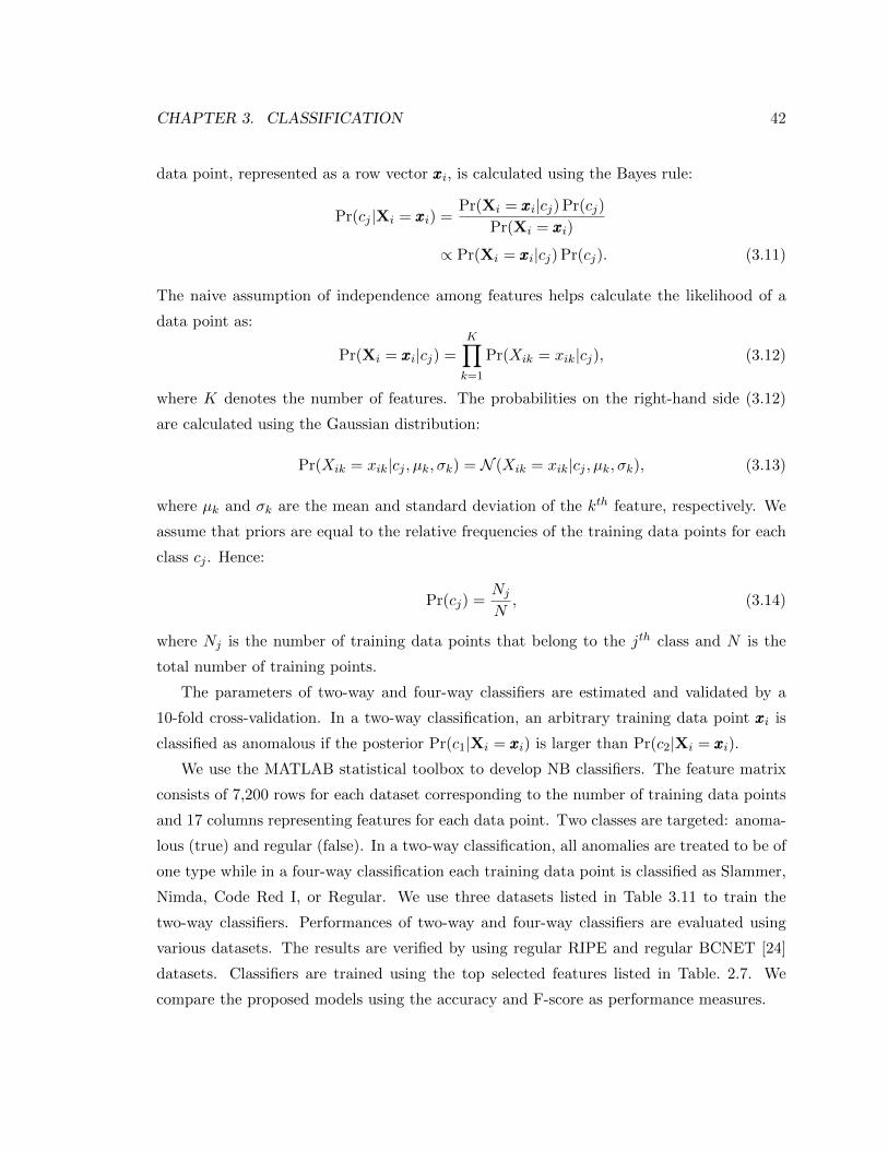
CHAPTER 3. CLASSIFICATION 42
data point, represented as a row vector xxxi, is calculated using the Bayes rule:
Pr(cj |Xi = xxxi) =Pr(Xi = xxxi|cj) Pr(cj)
Pr(Xi = xxxi)
∝ Pr(Xi = xxxi|cj) Pr(cj). (3.11)
The naive assumption of independence among features helps calculate the likelihood of a
data point as:
Pr(Xi = xxxi|cj) =
K∏k=1
Pr(Xik = xik|cj), (3.12)
where K denotes the number of features. The probabilities on the right-hand side (3.12)
are calculated using the Gaussian distribution:
Pr(Xik = xik|cj , µk, σk) = N (Xik = xik|cj , µk, σk), (3.13)
where µk and σk are the mean and standard deviation of the kth feature, respectively. We
assume that priors are equal to the relative frequencies of the training data points for each
class cj . Hence:
Pr(cj) =Nj
N, (3.14)
where Nj is the number of training data points that belong to the jth class and N is the
total number of training points.
The parameters of two-way and four-way classifiers are estimated and validated by a
10-fold cross-validation. In a two-way classification, an arbitrary training data point xxxi is
classified as anomalous if the posterior Pr(c1|Xi = xxxi) is larger than Pr(c2|Xi = xxxi).
We use the MATLAB statistical toolbox to develop NB classifiers. The feature matrix
consists of 7,200 rows for each dataset corresponding to the number of training data points
and 17 columns representing features for each data point. Two classes are targeted: anoma-
lous (true) and regular (false). In a two-way classification, all anomalies are treated to be of
one type while in a four-way classification each training data point is classified as Slammer,
Nimda, Code Red I, or Regular. We use three datasets listed in Table 3.11 to train the
two-way classifiers. Performances of two-way and four-way classifiers are evaluated using
various datasets. The results are verified by using regular RIPE and regular BCNET [24]
datasets. Classifiers are trained using the top selected features listed in Table. 2.7. We
compare the proposed models using the accuracy and F-score as performance measures.

CHAPTER 3. CLASSIFICATION 43
Table 3.11: The NB training datasets for the two-way classifiers.
NB Training dataset Test dataset
NB1 Slammer and Nimda Code Red INB2 Slammer and Code Red I NimdaNB3 Nimda and Code Red I Slammer
3.4.1 Two-Way Classification
The results of the two-way classification are shown in Table 3.12. The combination of Nimda
and Code Red I training data points (NB3) achieves the best classification results. The NB
models classify the training data points of regular RIPE and regular BCNET datasets with
95.8% and 95.5% accuracies, respectively. There are no anomalous data points in these
datasets and, thus, both TP and FN values are zero. Hence, the sensitivity (3.1) is not
defined and precision (3.2) is equal to zero. Consequently, the F-score (3.5) is not defined
for these cases and the accuracy (3.3) reduces to:
accuracy =TN
TN + FP. (3.15)
Classifiers trained based on features selected by the OR algorithms often achieve higher
accuracies and F-scores for training and test datasets listed in Table 3.11. The OR selection
algorithms perform well when used with the NB classifiers because the feature score (2.4)
is calculated using the probability distribution that the NB classifiers use for posterior
calculations (3.11). Hence, the features selected by the OR variants are expected to have a
stronger influence on the posteriors calculated by the NB classifiers [48]. The WOR feature
selection algorithm achieves the best F-score for all NB classifiers.
The test data points generated by various worms that are incorrectly classified in the two-
way classification (false positive and false negative) are shown in Figure 3.9 (left column).
The correctly classified traffic data points as anomaly (true positive) are shown in Figure 3.9
(right column).

CHAPTER 3. CLASSIFICATION 44
Table 3.12: Performance of the two-way naive Bayes classification.
Performance index
Accuracy (%) F-score (%)
No. NB Feature Test
dataset
(anomaly)
RIPE
(regular)
BCNET
(regular)
Test
dataset
(anomaly)
1 NB1 All features 87.6 91.1 77.3 2.31
2 NB1 Fisher 62.5 97.0 76.3 12.5
3 NB1 MID 72.3 93.1 82.3 26.9
4 NB1 MIQ 70.8 92.3 75.4 46.9
5 NB1 MIBASE 83.0 90.6 74.0 47.8
6 NB1 OR 52.0 80.4 85.3 43.9
7 NB1 EOR 53.1 81.1 77.7 39.2
8 NB1 WOR 97.5 87.1 77.1 48.0
9 NB1 MOR 62.6 80.9 79.8 34.3
10 NB1 CDM 55.1 94.0 82.6 16.4
11 NB2 All features 85.8 92.2 87.1 23.5
12 NB2 Fisher 64.2 97.5 89.0 4.87
13 NB2 MID 70.3 94.3 95.0 10.7
14 NB2 MIQ 85.7 94.0 90.0 22.9
15 NB2 MIBASE 87.9 92.1 87.2 23.1
16 NB2 OR 69.4 81.2 90.4 23.2
17 NB2 EOR 67.1 81.8 89.8 18.4
18 NB2 WOR 70.7 88.3 86.9 35.8
19 NB2 MOR 73.9 81.9 90.6 25.2
20 NB2 CDM 77.5 94.3 93.0 21.5
21 NB3 All features 89.1 91.8 85.9 53.2
22 NB3 Fisher 77.1 92.5 85.9 19.8
23 NB3 MID 76.6 45.2 92.5 46.1
24 NB3 MIQ 90.4 91.8 87.2 63.5
25 NB3 MIBASE 82.9 91.3 86.1 57.6
26 NB3 OR 45.9 76.3 88.1 55.6
27 NB3 EOR 63.3 78.8 88.9 61.3
28 NB3 WOR 83.1 88.1 86.3 60.3
29 NB3 MOR 58.6 81.6 89.2 59.8
30 NB3 CDM 46.3 95.6 91.9 32.5

CHAPTER 3. CLASSIFICATION 45
01/25 01/270
1
2
3
4
5x 10
4
Time
Nu
mb
er
of
IGP
pa
cke
ts Slammer
Red: FP and FN
Blue: TP and TN
01/25 01/270
1
2
3
4
5x 10
4
Time
Nu
mb
er
of
IGP
pa
cke
ts
Slammer
Red: TP
Blue: TN, FN, and FP
09/20 09/220
0.5
1
1.5
2
x 104
Time
Nu
mb
er
of
IGP
pa
cke
ts Nimda
Red: FP and FN
Blue: TP and TN
09/20 09/220
0.5
1
1.5
2
x 104
Time
Nu
mb
er
of
IGP
pa
cke
ts Nimda
Red: TP
Blue: TN, FN, and FP
07/230
0.5
1
1.5
2
x 104
Time
Nu
mb
er
of
IGP
pa
cke
ts
Code Red I
Red: FP and FN
Blue: TP and TN
07/230
0.5
1
1.5
2
x 104
Time
Nu
mb
er
of
IGP
pa
cke
ts
Code Red I
Red: TP
Blue: TN, FN, and FP
Figure 3.9: Shown in red are incorrectly classified regular and anomaly traffic for Slammer
(top left), Nimda (middle left), and Code Red I (bottom left); and correctly classified
anomaly traffic for Slammer (top right), Nimda (middle right), and Code Red I (bottom
right)
3.4.2 Four-Way Classification
The four-way classification results are shown in Table 3.13. The four-way NB model classifies
data points as Slammer, Nimda, Code Red I, or Regular. Both regular RIPE and regular
BCNET datasets are tested. The regular BCNET dataset classification results are also

CHAPTER 3. CLASSIFICATION 46
listed in order to verify the performance of the proposed classifiers. Although it is difficult
to classify four distinct classes. The classifier trained based on the features selected by the
MOR algorithm achieves 68.7% accuracy.
Table 3.13: Accuracy of the four-way naive Bayes classification.
Average accuracy (%)
3 anomalies concatenated with
1 regular
No. Feature set RIPE BCNET
1 All features 74.3 67.6
2 Fisher 24.7 34.3
3 MID 74.9 33.1
4 MIQ 24.6 34.8
5 MIBASE 75.4 33.1
6 OR 25.5 36.7
7 EOR 75.3 68.1
8 WOR 75.8 53.2
9 MOR 77.7 68.7
10 CDM 24.8 34.5
Performance of the NB classifiers is often inferior to the SVM and HMM classifiers [49], [50].
However, the NB2 classifier trained on the Slammer and Code Red I datasets (F-score =
32.1%) performs better than the SVM classifier (F-score = 22.2%).

Chapter 4
BGPAD Tool
We develop a graphical user interface for the MATLAB code to allow the users to inspect
BGP packets for anomalies. It supports both PCAP and MRT formats. A complete code
for the tool is available [26]. BGPAD tool provides the following functionalities:
• An option to convert a MRT ASCII format to feature set file.
• An option to convert a PCAP ASCII format to feature set file.
• Generated statistics of various features for any BGP trace.
• Test performance indices and displays anomalous traffic.
• An option to select classification two-way or four-way classification algorithms (SVM,
HMM, and NB).
• An option to parametrize each algorithm and to achieve the best performance.
• An option to upload PCAP files to be tested on the trained models [49].
• An option to save the results as tables and graphs.
The feature set file is an input file that is formatted so that rows correspond to traffic data
points and columns correspond to values of the extracted features.
47

CHAPTER 4. BGPAD TOOL 48
The extracted feature values along with their distribution for various datasets are shown
in Figure 4.1. BGPAD provides the functionality to change the number of the bins of the
distribution and to save the graphs to the user local machine.
Code Red I Code Red I
Figure 4.1: Inspection of BGP PCAPs and MRT files statistics.
The SVM two-way classification’s GUI is shown in Figure 4.2. It provides full control
of SVM parameters including C, γ, and the number of folds for cross-validation. It also
provides an option to choose the feature selection algorithm. Various test datasets are
available including the test datasets listed in Table 2.2. BGPAD permits to upload a test
dataset to evaluate the proposed SVM models. Various performance indices are shown after
the testing is completed. The GUI also allows the user to generate and save the graphs of
false negatives/false positives and the true positives. The Test button provides an option
to evaluate a test dataset based on the best trained SVM model [49].

CHAPTER 4. BGPAD TOOL 49
Figure 4.2: GUI for two-way SVM models.

CHAPTER 4. BGPAD TOOL 50
The generated graphs of Slammer, Nimda, and Code Red I test datasets used along with
training datasets (Table 3.2) are shown in Figure 4.3. Shown in red are incorrectly classified
regular and anomaly traffic for Slammer (top left), Nimda (top right), and Code Red I (top
middle) and correctly classified anomaly traffic for Slammer (bottom left), Nimda (bottom
right), and Code Red I (bottom middle).
Figure 4.3: Two-way SVM graphs.
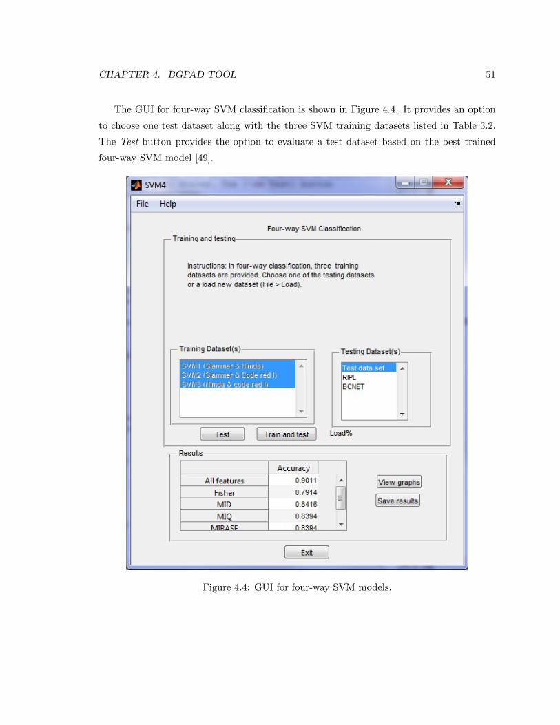
CHAPTER 4. BGPAD TOOL 51
The GUI for four-way SVM classification is shown in Figure 4.4. It provides an option
to choose one test dataset along with the three SVM training datasets listed in Table 3.2.
The Test button provides the option to evaluate a test dataset based on the best trained
four-way SVM model [49].
Figure 4.4: GUI for four-way SVM models.

CHAPTER 4. BGPAD TOOL 52
HMM two-way classification GUI is shown in Figure 4.5. In two-way classification, a
five training datasets are provided. The user has an option to choose three anomalous
training datasets and one regular. The regular dataset options are BCNET or RIPE. The
test datasets should also contain three anomalies and one regular dataset. The GUI also
provides an option to choose one of the feature selection algorithms and the number of hidden
states. The Test button evaluates a test dataset on the best trained HMM model [49].
Figure 4.5: GUI for two-way HMM models.

CHAPTER 4. BGPAD TOOL 53
The HMM four-way classification GUI is shown in Figure 4.6. In four-way classification,
a five training datasets are provided from which four datasets should be selected. The GUI
provides an option to choose one of the three anomalous datasets and one regular testing
dataset (BCNET, RIPE, or user specific dataset).
Figure 4.6: GUI for four-way HMM models.

CHAPTER 4. BGPAD TOOL 54
Two-way and four-way NB classification GUIs are shown in Figure 4.7 and Figure 4.8,
respectively. The available options are similar to those in SVM classification GUI.
Figure 4.7: GUI for two-way NB models.

CHAPTER 4. BGPAD TOOL 55
Figure 4.8: GUI for four-way NB models.

Chapter 5
Analysis of Classification Results
and Discussion
Performance of the BGP is based on trust among BGP peers because they assume that the
interchanged announcements are accurate and reliable. This trust relationship is vulnerable
during BGP anomalies. For example, during BGP hijacks, a BGP peer may announce
unauthorized prefixes that indicate to other peers that it is the originating peer. These
false announcements propagate across the Internet to other BGP peers and, hence, affect
the number of BGP announcements (updates and withdrawals) worldwide. This storm of
BGP announcements affects the quantity of volume features. As shown in Table 2.5, 65% of
the selected features are volume features. Hence, volume features are more relevant to the
anomaly class than the AS-path features, which confirms the known effect of BGP anomalies
on the volume of the BGP announcements. To illustrate the effect of volume features and
AS-path features, we apply two-way SVM classification separately with volume and with
AS-path features. The results are shown in Table 5.1.
The top selected AS-path features that appear on the boundaries of the distributions
are shown in Figure 2.3. For example, AS-path features 24, 25, and 32 have the highest
MIQ, Fisher, and MID scores, respectively. This indicates that during BGP anomalies, the
edit distance and AS-PATH length of the BGP announcements tend to have a very high or
a very low value and, hence, large variance. This implies that during an anomaly attack,
AS-path features are the distribution outliers.
56

CHAPTER 5. ANALYSIS OF CLASSIFICATION RESULTS AND DISCUSSION 57
Table 5.1: Comparison of feature categories in two-way SVM classification.
Performance index
SVM Category Accuracy Precision Sensitivity Specificity Balanced accuracy F-score
SVM1 volume 68.5 53.6 16.6 73.2 44.9 27.1
SVM1 AS-path 56.4 6.12 29.5 58.8 44.1 3.93
SVM2 volume 87.0 69.6 12.5 99.1 55.8 22.3
SVM2 AS-path 86.0 38.7 1.19 99.6 50.4 2.36
SVM3 volume 94.8 79.7 76.4 97.3 86.8 85.0
SVM3 AS-path 56.9 19.1 79.4 53.8 66.6 64.1
Approximately 58% of the AS-path features shown in Table 2.5 are larger than the
distribution mean. For example, large length of the AS-PATH BGP attribute implies that
the packet is routed via a longer path to its destination, which causes large routing delays
during BGP anomalies [32]. In a similar case, very short lengths of AS-PATH attributes
occur during BGP hijacks when the new (false) originator usually gains a preferred or shorter
path to the destination [51]. The SVM models exhibit better performance than the HMMs
in two-way and four-way classifications. The SVM models based on Nimda and Code Red I
datasets and the HMMs with two hidden states have the highest accuracies. HMMs based on
the number of announcements and number of withdrawals (feature 1 and feature 2) achieve
better accuracy in two-way and four-way classifications than models based on the maximum
number of AS-PATH length (feature 6) and the maximum edit distance (feature 12). Both
SVM and HMM two-way classifications produced better results than four-way classifications
because of the common semantics among BGP anomalies. For example, Slammer worm is
more correlated to Nimda than to regular RIPE mapped sequence.
We compare the proposed results to rule-based and behavioural techniques by comparing
the proposed models with models proposed in the research literature. Table 5.2 illustrates
that using rule-based technique [52], the classifier performs worse than the proposed models
in two datasets (Nimda and Code Red I) out of three datasets. However, the proposed mod-
els achieve better accuracy compared to behavioural techniques [53]. The shaded columns
show that the model does not consider the difference among the three anomalies. Instead,
it takes into account that the dataset is anomaly rather than specifying the type of anomaly
(Slammer, Nimda, and Code Red I). Although it is difficult to make fair comparison be-
cause of the differences between the datasets class ranges, feature selection algorithms, and

CHAPTER 5. ANALYSIS OF CLASSIFICATION RESULTS AND DISCUSSION 58
dataset sources, models proposed in this thesis show better overall results than the two
models reported in the literature. It is also important to mention that, to the best of our
knowledge, there are no proposed multi-classification models of BGP worms reported in the
literature.
Table 5.2: Performance comparison of anomaly detection models.
Proposed models
Dataset SVM
two-way
SVM
four-way
HMM
two-way
HMM
four-way
NB
two-way
NB
four-way
Rule-based
techniques
Behavioural
techniques
Slammer 89.3 82.8 86.0 70.0 87.4 77.7 94.4 74.0
Nimda 68.6 82.8 86.0 70.0 70.1 77.7 84.1 74.0
Code Red I 79.1 82.8 86.0 70.0 74.1 77.7 74.9 74.0
The development of the proposed models greatly depends on several factors:
• Domain experts involvement: Most labeling assumptions for the BGP worms datasets
are based on the technical reports that were released after the worm attacks. There are
no agreed time limits to label the data points. In this thesis, we rely on the literature
reviews [4] and the visual effect of worms on volume features to decide the limits for
each dataset.
• Confidentiality of data: Most Internet service providers restrict the access to the
collected BGP traffic. Most application layer protocols contain confidential user infor-
mation. These application layer packets are confidential because they contain private
information about the Internet users. Anonymization tools may remove these privacy
concerns.
• The Internet rapid development: Due to the fast development of the Internet services,
many legitimate traffic data points are captured by the proposed models as anomalous
traffic. Hence, a periodic training may be necessary to adapt the proposed models to
these new services [11].
Chapter 6
Conclusions
In this thesis, we have analysed BGP anomalies such as Slammer, Nimda, and Code Red I.
We compare feature selection algorithms to choose the most correlated features for anomaly
class. We introduce new classification features and apply various machine learning algo-
rithms. The proposed models show better performance compared to models proposed in
the literature.
We have investigated BGP anomalies and proposed detection models based on the SVM,
HMM, and NB classifiers. Classification results show that the best achieved F-scores of the
SVM, HMM, and NB models are 86.1%, 84.4%, and 69.7%, respectively. Furthermore,
volume mapped sequences generate models with better accuracy than AS-path mapped
sequences. Hence, using the BGP volume features is a viable approach for detecting possible
worm attacks. The extracted features share similar statistical semantics and, hence, are
grouped into two categories. Since BGP anomalies have similar properties and effect on
BGP features, the proposed models may be used as online mechanisms to predict new BGP
anomalies and detect the onset of worm attacks.
Further investigation of the effect of anomalies and worms on BGP may lead to a bet-
ter feature extraction process. Furthermore, applying better feature selection algorithms
may generate more correlated features of the anomaly class and, hence, may improve the
performance of the detection models. Further analysis on the results may lead to better
understanding of the performance indices. For example, receiver operating characteristic
(ROC) analysis may generate better performance measure than the F-score index. ROC
curve shows the relationship between false positive and true positive ratios for various pa-
rameters of the machine learning model. An online version of BGPAD tool is developed to
59

CHAPTER 6. CONCLUSIONS 60
provide a web interface for the end users [26]. Spatio-temporal network anomaly detection is
one of the proposed models to build the online system because it takes in consideration the
dependency of the data points among each other [54]. Spatio-temporal statistical approach
may discover new anomalies that are not present in the training dataset.

References
[1] Y. Rekhter and T. Li, A Border Gateway Protocol 4 (BGP-4). RFC 1771, IETF, Mar.
1995.
[2] S. Lally, T. Farah, R. Gill, R. Paul, N. Al-Rousan, and Lj. Trajkovic, “Collection and
characterization of BCNET BGP traffic,” in Proc. 2011 IEEE Pacific Rim Conf. on
Communications, Computers and Signal Processing, Victoria, BC, Canada, Aug. 2011,
pp. 830–835.
[3] Internet Assigned Numbers Authority [Online]. Available: http://www.iana.org/.
[4] S. Deshpande, M. Thottan, T. K. Ho, and B. Sikdar, “An online mechanism for BGP
instability detection and analysis,” IEEE Trans. Computers, vol. 58, no. 11, pp. 1470–
1484, Nov. 2009.
[5] J. Li, D. Dou, Z. Wu, S. Kim, and V. Agarwal, “An Internet routing forensics framework
for discovering rules of abnormal BGP events,” SIGCOMM Comput. Commun. Rev.,
vol. 35, no. 4, pp. 55–66, Oct. 2005.
[6] Slammer: Why security benefits from proof of concept code [Online]. Available: http:
//www.theregister.co.uk/2003/02/06/slammer why security benefits/.
[7] W32.SQLExp.Worm [Online]. Available: http://www.symantec.com/security
response/writeup.jsp?docid=2003-012502-3306-99.
[8] Advisory CA-2001-26 Nimda Worm [Online]. Available: http://www.cert.org/
advisories/CA-2001-26.html.
[9] ANALYSIS: .ida Code Red Worm [Online]. Available: http://www.eeye.com/
Resources/Security-Center/Research/Security-Advisories/AL20010717.
61
REFERENCES 62
[10] J. Zhang, J. Rexford, and J. Feigenbaum, “Learning-based anomaly detection in BGP
updates,” in Proc. Workshop on Mining Network Data, Philadelphia, PA, USA, May
2005, pp. 219–220.
[11] P. Winter, E. Hermann, and M. Zeilinger, “Inductive intrusion detection in flow-based
network data using one-class support vector machines,” in New Technologies, Mobility
and Security (NTMS), 2011 4th IFIP Int. Conf., Paris, France, Feb. 2011, pp. 1–5.
[12] V. Chandola, A. Banerjee, and V. Kumar, “Anomaly detection: a survey,”
ACM Comput. Surv., vol. 41, no. 3, pp. 1–58, July 2009. [Online]. Available:
http://doi.acm.org/10.1145/1541880.1541882.
[13] M. Thottan, G. Liu, and C. Ji., “Anomaly detection approaches for communication
networks,” in Algorithms for Next Generation Networks, Springer, London, Sept. 2010,
pp. 239–261.
[14] H. Hajji, “Statistical analysis of network traffic for adaptive faults detection,” IEEE
Trans. on Neural Networks, vol. 16, no. 5, pp. 1053–1063, Sept. 2005.
[15] P.-N. Tan, M. Steinbach, and V. Kumar, Introduction to Data Mining, 1st ed. Boston,
MA, USA: Addison-Wesley Longman Publishing Co., Inc., 2005.
[16] M. F. Augusteijn and B. A. Folkert, “Neural network classification and novelty
detection,” International Journal of Remote Sensing, vol. 23, no. 14, pp. 2891–2902,
Mar. 2002.
[17] I. Diaz and J. Hollmen, “Residual generation and visualization for understanding novel
process conditions,” in Proc. Neural Networks. IJCNN ’02, vol. 3, no. 3, pp. 2070–2075,
May 2002.
[18] M. Negnevitsky, Artificial Intelligence: A Guide to Intelligent Systems, 1st ed. Boston,
MA, USA: Addison-Wesley Longman Publishing, 2001.
[19] O. Sharma, M. Girolami, and J. Sventek, “Detecting worm variants using machine
learning,” in Proc. ACM CoNEXT Conf., New York, NY, USA: ACM, Dec. 2007, pp.
1–12.

REFERENCES 63
[20] A. A. Sebyala, T. Olukemi, L. Sacks, and D. L. Sacks, “Active platform security through
intrusion detection using naive bayesian network for anomaly detection,” in Proc. Lon-
don Communications Symposium, London, May 2002, pp. 15–18.
[21] A. W. Moore and D. Zuev, “Internet traffic classification using Bayesian analysis
techniques,” in Proc. Int. Conf. on Measurement and Modeling of Computer Systems,
Banff, AB, Canada, May 2005, pp. 50–60.
[22] K. El-Arini and K. Killourhy, “Bayesian detection of router configuration anomalies,”
in Proc. of Workshop on Mining Network Data, Philadelphia, PA, USA, June 2005, pp.
221–222.
[23] RIPE RIS raw data [Online]. Available: http://www.ripe.net/data-tools/stats/ris/
ris-raw-data.
[24] BCNET [Online]. Available: http://www.bc.net.
[25] J. Chen, H. Huang, S. Tian, and Y. Qu, “Feature selection for text classification with
naive Bayes,” Expert Systems with Applications, vol. 36, no. 3, pp. 5432–5435, Apr.
2009.
[26] BGPAD tool [Online]. Available: www.sfu.ca/∼ljilja/cnl/projects/BGPAD.
[27] University of Oregon Route Views project [Online]. Available: http://www.routeviews.
org/.
[28] T. Manderson, “Multi-threaded routing toolkit (MRT) border gateway protocol (BGP)
routing information export format with geo-location extensions,” RFC 6397, IETF,
Oct. 2011 [Online]. Available: http://www.ietf.org/rfc/rfc6397.txt.
[29] Zebra BGP parser [Online]. Available: http://www.linux.it/∼md/software/
zebra-dump-parser.tgz.
[30] T. Farah, S. Lally, R. Gill, N. Al-Rousan, R. Paul, D. Xu, and Lj. Trajkovic, “Col-
lection of BCNET BGP traffic,” in Proc. 23rd International Teletraffic Congress, San
Francisco, CA, USA, Sept. 2011, pp. 322–323.
[31] D. Meyer, “BGP communities for data collection,” RFC 4384, IETF, 2006 [Online].
Available: http://www.ietf.org/rfc/rfc4384.txt.

REFERENCES 64
[32] L. Wang, X. Zhao, D. Pei, R. Bush, D. Massey, A. Mankin, S. F. Wu, and L. Zhang,
“Observation and analysis of BGP behavior under stress,” in Proc. 2nd ACM SIG-
COMM Workshop on Internet Measurment, New York, NY, USA, May 2002, pp. 183–
195.
[33] G. H. John, R. Kohavi, and K. Pfleger, “Irrelevant features and the subset selection
problem,” in Proc. Int. Conf. on Machine Learning, New Brunswick, NJ, USA, July
1994, pp. 121–129.
[34] Y.-W. Chen and C.-J. Lin, “Combining SVMs with various feature selection strategies,”
in Feature Extraction: Foundations and Applications, London, Springer, June 2006, pp.
317–328.
[35] Q. Gu, Z. Li, and J. Han, “Generalized fisher score for feature selection,” in Proc. Conf.
on Uncertainty in Artificial Intelligence, Barcelona, Spain, July 2011, pp. 266–273.
[36] H. Peng, F. Long, and C. Ding, “Feature selection based on mutual information cri-
teria of max-dependency, max-relevance, and min-redundancy,” IEEE Trans. Pattern
Analysis and Machine Intelligence, vol. 27, no. 8, pp. 1226–1238, Aug. 2005.
[37] J. Wang, X. Chen, and W. Gao, “Online selecting discriminative tracking features
using particle filter,” in Proc. Computer Vision and Pattern Recognition, volume 2,
San Diego, CA, USA, June 2005, pp. 1037–1042.
[38] T. Ahmed, B. Oreshkin, and M. Coates. “Machine learning approaches to network
anomaly detection,” in Proc. USENIX Workshop on Tackling Computer Systems Prob-
lems with Machine Learning Techniques, Cambridge, MA, May 2007, pp. 1–6.
[39] G. J. McLachlan, K. A. Do, and C. Ambroise, Microarrays in Gene Expression
Studies. Hoboken, NJ, USA: John Wiley & Sons, Inc., 2005, pp. 1–29.
[40] X. Song, M. Wu, C. Jermaine, and S. Ranka, “Conditional anomaly detection,” IEEE
Trans. on Knowl. and Data Eng., vol. 19, no. 5, pp. 631–645, May 2007.
[41] Support Vector Machine - The Book [Online]. Available: http://www.support-vector.
net/chapter 6.html.

REFERENCES 65
[42] A. L. Goldberger, L. A. N. Amaral, L. Glass, J. M. Hausdorff, P. C. Ivanov, R. G.
Mark, J. E. Mietus, G. B. Moody, C.-K. Peng, and H. E. Stanley, “Physiobank,
physiotoolkit, and physionet: components of a new research resource for complex
physiologic signals,” Circulation, vol. 101, no. 23, pp. e215–e220, June 2000.
[43] Libsvm–a library for support vector machines [Online]. Available: http://www.csie.
ntu.edu.tw/∼cjlin/libsvm/.
[44] C. M. Bishop, Pattern Recognition and Machine Learning. Secaucus, NJ, USA:
Springer-Verlag, Aug. 2006, p. 36, p. 327.
[45] T. Ahmed, M. Coates, and A. Lakhina, “Multivariate online anomaly detection using
kernel recursive least squares,” in Proc. 26th IEEE International Conf. on Computer
Communications, Mar. 2007, pp. 625–633.
[46] C.-W. Hsu and C.-J. Lin, “A comparison of methods for multiclass support vector
machines,” IEEE Trans. Neural Networks, vol. 13, no. 2, pp. 415–425, Mar. 2002.
[47] J. D. Gardiner, “Multiple Markov models for detecting Internet anomalies from BGP
data,” in Proc. DoD High Performance Computing Modernization Program Users
Group Conf., Washington, DC, USA, June 2009, pp. 374–377.
[48] D. Mladenic and M. Grobelnik, “Feature selection for unbalanced class distribution
and naive Bayes,” in Proc. Int. Conf. Machine Learning, Bled, Slovenia, June 1999,
pp. 258–267.
[49] N. Al-Rousan and Lj. Trajkovic, “Machine learning models for classification of BGP
anomalies,” in Proc. IEEE Conf. High Performance Switching and Routing, HPSR
2012, Belgrade, Serbia, June 2012, pp. 103–108.
[50] N. Al-Rousan, S. Haeri, and Lj. Trajkovic, “Feature selection for classification of BGP
anomalies using Bayesian models,” in Proc. ICMLC 2012, Xi’an, China, July 2012.
[51] YouTube Hijacking: A RIPE NCC RIS case study [Online]. Avail-
able: http://www.ripe.net/internet-coordination/news/industry-developments/
youtube-hijacking-a-ripe-ncc-ris-case-study.

REFERENCES 66
[52] R. Moskovitch, Y. Elovici, and L. Rokach, “Detection of unknown computer worms
based on behavioral classification of the host abstract,” in Proc. Computational Intel-
ligence in Security and Defense Applications, Milan, Italy, May 2007, pp. 110–113.
[53] D. Dou, J. Li, H. Qin, and S. Kim, “S.: Understanding and utilizing the hierarchy of ab-
normal BGP events,” in Proc. SIAM International Conf. on Data Mining, Minneapolis,
MN, USA, Apr. 2007, pp. 457–462.
[54] A. Dainotti, A. Pescape, and K. Claffy, “Issues and future directions in traffic classifi-
cation,” IEEE Network, vol. 58, no. 11, pp. 35–40, Jan. 2012.

Appendix A
Parameter Assumptions
Table A.1 shows the parameters used in this Thesis.
Table A.1: Sample of a BGP update packet.
Parameter Value Explanation
Number of portions in HMM mapping function 11 Heuristic
Number of HMMs 6, 12 All combinations of three values of
hidden states and four datasets
in two-way and four-way classifications
Number of folds in cross-validation 10 Heuristic
Number of SVM features 37 The total number of defined features
Number of features per HMM observation sequence 2 Arbitrary chosen. More accurate results may be
achieved by performing cross-validations
Number of NB features 17 Using continuous and categorical features gives better
results than using the combination of continuous, cat-
egorical, and binary features
Number of the top selected features 10 Heuristic
67