comparison of one-dimensional hec-ras with two-dimensional

Comparison of one-dimensional HEC-RAS with two-dimensional FESWMS model in flood inundation mapping

A Thesis

Submitted to the Faculty

of

Purdue University

by

Aaron Christopher Cook

In Partial Fulfillment of the

Requirements for the Degree

of

Master of Science in Civil Engineering

May 2008

Purdue University

West Lafayette, Indiana

ii

To my parents, my dog, and the rest of my family.

iii

ACKNOWLEDGMENTS

The data for this study was provided by the North Carolina Floodplain Mapping Program

(NCFMP) and Fort Bend County, Texas. This study would not have been possible

without this data.

I would like to thank my advisor Dr. Venkatesh Merwade for all his support and time. I

would also like to thank my committee members Dr. Rao Govindaraju and Dr. Dennis

Lyn.

Finally, I would like to thank my officemates Emily, Jared, Mark, Megan and Young Hun

and the rest of the Hydraulic/Hydrology Group.

iv

TABLE OF CONTENTS

Page LIST OF TABLES ............................................................................................................ vii

LIST OF FIGURES ......................................................................................................... viii

ABBREVIATIONS ............................................................................................................ x

ABSTRACT ....................................................................................................................... xi

CHAPTER 1. INTRODUCTION ....................................................................................... 1

1.1. Introduction .............................................................................................................. 1

1.2. Approach .................................................................................................................. 2

1.3. Thesis Organization .................................................................................................. 3

CHAPTER 2. LITERATURE REVIEW ............................................................................ 4

2.1. Introduction .............................................................................................................. 4

2.2. Comparison of 1D and 2D hydraulic models ........................................................... 4

2.2.1. HEC-RAS ........................................................................................................... 5

2.2.2. FESWMS ........................................................................................................... 8

2.2.3. Case studies using 1D hydraulic models .......................................................... 11

2.2.4. Case studies using 2D hydraulic models .......................................................... 11

2.2.5. Case studies comparing 1D and 2D hydraulic models ..................................... 12

2.2.6. Combined 1D-2D hydraulic models ................................................................ 14

2.3. Effects of topography on hydraulic models ............................................................ 15

2.3.1. DEM Resolution ............................................................................................... 16

2.3.2. DEM Accuracy ................................................................................................. 18

2.4. Effects of geometry on hydraulic models ............................................................... 18

2.4.1. Effect of 1D geometry on hydraulic models .................................................... 19

2.4.2. Effect of 2D geometry on hydraulic models .................................................... 20

v

Page

2.5. Model Parameters ................................................................................................... 21

2.6. Summary ................................................................................................................. 24

CHAPTER 3. STUDY AREA AND DATA .................................................................... 25

3.1. Introduction ............................................................................................................ 25

3.2. Description of Strouds Creek ................................................................................. 25

3.2.1. Cross-section and Bridge Data ......................................................................... 26

3.2.2. Flow Data ......................................................................................................... 27

3.3. Description of the Brazos River ............................................................................. 28

3.3.1. Cross-section and Bridge Data ......................................................................... 29

3.3.2. Flow Data ......................................................................................................... 31

3.4. Light Detection and Ranging Elevation Data ......................................................... 31

3.5. National Elevation Dataset ..................................................................................... 32

3.6. Integrated Dataset ................................................................................................... 32

CHAPTER 4. METHODOLOGY .................................................................................... 33

4.1. Introduction ............................................................................................................ 33

4.2. 1D floodplain mapping using HEC-RAS ............................................................... 33

4.2.1. Strouds Creek Cross-sectional Modifications .................................................. 35

4.2.2. Brazos River Cross-sectional Modification ..................................................... 38

4.2.3. Topographic Representation ............................................................................ 41

4.2.4. Flow Data and Simulation ................................................................................ 42

4.2.5. Flood Inundation Mapping ............................................................................... 42

4.3. 2D floodplain mapping using FESWMS for Strouds Creek .................................. 42

4.3.1. Strouds Creek Mesh Resolution ....................................................................... 43




4.4. 2D floodplain mapping using FESWMS for the Brazos River .............................. 45

4.4.1. Brazos River Mesh Resolution ......................................................................... 47


vi

Page



CHAPTER 5. RESULTS .................................................................................................. 49

5.1. Introduction ............................................................................................................ 49

5.2. Effect of Topography on one-dimensional hydraulic model .................................. 49

5.2.1. Strouds Creek ................................................................................................... 49

5.2.2. Brazos River ..................................................................................................... 53

5.3. Effect of Geometry on one-dimensional hydraulic model ..................................... 56

5.3.1. Strouds Creek ................................................................................................... 56

5.3.2. Brazos River ..................................................................................................... 62

5.4. Effect of Topography on the two-dimensional hydraulic model ............................ 66

5.4.1. Strouds Creek ................................................................................................... 66

5.4.2. Brazos River ..................................................................................................... 68

5.5. Effect of Geometry on two-dimensional hydraulic model ..................................... 70

5.5.1. Strouds Creek ................................................................................................... 70

5.5.2. Brazos River ..................................................................................................... 71

5.6. Comparison of HEC-RAS and FESWMS .............................................................. 72

5.6.1. Strouds Creek ................................................................................................... 72

5.6.2. Brazos River ..................................................................................................... 76

CHAPTER 6. SUMMARY AND CONCLUSIONS ........................................................ 79

6.1. Effect of topography on 1D and 2D hydraulic models ........................................... 79

6.2. Effect of geometry on 1D and 2D hydraulic models .............................................. 80

6.3. Comparison of 1D and 2D Hydraulic Models ........................................................ 81

6.4. Future Work ............................................................................................................ 82

LIST OF REFERENCES .................................................................................................. 84

APPENDIX – TUTORIAL ON USING SMS 9.2 - CD-ROM INCLUDED

vii

LIST OF TABLES

Table Page 3.1 Flow Rates for Strouds Creek ..................................................................................... 28

3.2 Flow Rates for Brazos River ....................................................................................... 31

4.1 Description of the Cross-sectional Configurations for Strouds Creek ........................ 36

4.2 Description of the Cross-sectional Configurations for the Brazos River ................... 39

5.1 Inundation for Original Cross-sections ....................................................................... 50

5.2 Inundation for Original Cross-sections ....................................................................... 53

5.3 Inundation Area (mi2) (% Change) ............................................................................. 57

5.4 Average Width of Inundation (ft) ............................................................................... 61


5.6 Average Width of Inundation (mi) ............................................................................. 65

5.7 Inundation for the 10 ft mesh resolution ..................................................................... 66

5.8 Inundation for the 125 ft mesh resolution ................................................................... 68


5.10 Average Width of Inundation (ft) ............................................................................. 71

5.11 Inundation Area (mi2) (% Change) ........................................................................... 71

5.12 Average Width of Inundation (mi) ........................................................................... 72

5.13 Inundation Area (mi2) ............................................................................................... 73

5.14 Average Width of Inundation (ft) ............................................................................. 75

5.15 Inundation Area (mi2) ............................................................................................... 76

viii

LIST OF FIGURES

Figure Page 3.1 Strouds Creek Study Area ........................................................................................... 26

3.2 Brazos River Study Area ............................................................................................ 29

4.1 HEC-GeoRAS configuration for a) Strouds Creek b) Brazos River .......................... 34

4.2 Strouds Creek Cross-Sections Removed .................................................................... 37

4.3 Strouds Creek Cross-Sectional Configuration ............................................................ 38

4.4 Brazos River Cross-Sections Removed ..................................................................... 40

4.5 Brazos River Cross-Sectional Configuration ............................................................. 41

4.6 Strouds Creek mesh resolution in SMS a) 10 foot b) 20 foot ..................................... 43

4.7 Brazos River mesh resolution in SMS a) 125 foot b) 250 foot ................................... 47

5.1 Inundation Boundary for a) Entire Reach; b) Magnified to a Bend in the River ........ 51

5.2 Cross-section Station 7986.1 for the a) Integrated; b) LiDAR DEM ......................... 52

5.3 Inundation Boundary for a) Entire Reach; b) Magnified to the Levees ..................... 54

5.4 Inundation Boundary for Original Cross-sections for the Integrated and LiDAR DEMs ............................................................................................................ 55

5.5 Cross-section Station 143373.8 for a) Integrated; b) LiDAR DEM ........................... 56

5.6 Inundation Boundary for the Integrated DEM for a) Entire Reach; b) Magnified Section for Four Cross-Sectional Modifications .................................. 59

5.7 Inundation Boundary for the NED 30 m DEM for a) Entire Reach; b) Magnified Section for Four Cross-Sectional Modifications .................................. 60

5.8 Inundation Boundary for the NED 30 m DEM for a) Entire Reach; b) Magnified Section for Four Cross-Sectional Modifications ................................. 63

5.9 Inundation Boundary for the NED 30 m DEM for a) Entire Reach; b) Magnified Section for Four Cross-Sectional Modifications .................................. 64

5.10 Inundation Boundary for a) Entire Reach; b) Magnified to a Bend in the River for the FESWMS 10 foot mesh resolution. ........................................... 67

ix

Page 5.11 Inundation Boundary for 125 ft Mesh Resolution for a) Entire Reach; b) Upstream Section ....................................................................................... 69

5.12 Cross-section showing large bank on south side of the Brazos River ...................... 70

5.13 Inundation Boundary for 10 ft Mesh Resolution and a) S; b) SA1; c) SR1; d) SR2 for the Integrated DEM ..................................................................... 74

5.14 Inundation Boundary for 10 ft Mesh Resolution and a) S; b) SA1; c) SR1; d) SR2 for the NED 30 m DEM ................................................................... 75

5.15 Inundation Boundary for 125 ft Mesh Resolution and a) S; b) SA1; c) SR1; d) SR2 for the Integrated DEM ..................................................................... 77

5.16 Inundation Boundary for 125 ft Mesh Resolution and a) S; b) SA1; c) SR1; d) SR2 for the NED 30 m DEM .................................................................... 78

x

ABBREVIATIONS

1D One-dimensional 2D Two-dimensional ASCII American Standard Code for Information Interchange DEM Digital Elevation Model DTM Digital Terrain Model DFIRM Digital Flood Insurance Rate Map FEMA Federal Emergency Management Agency FESWMS Finite-Element Surface-Water Modeling System FST2DH Depth-Averaged Flow and Sediment Transport Model GIS Geographic Information System HEC-RAS Hydrologic Engineering Center River Analysis System IfSAR Interferometric Synthetic Aperture Radar LiDAR Light Detection and Ranging NED National Elevation Data RMSE Root Mean Squared Error SMS Surface-water Modeling System SRTM Shuttle Radar Topography Mission USGS United States Geological Survey

xi

ABSTRACT

Cook, Aaron Christopher. MSCE, Purdue University, May, 2008. Comparison of one-dimensional HEC-RAS with two-dimensional FESWMS model in flood inundation mapping. Major Professor: Venkatesh Merwade. Flood inundation mapping is influenced by many factors such as the quality of terrain

data (digital elevation model, DEM), the cross-sectional configuration, and the use of a

one (1D) or two-dimensional (2D) hydraulic model. The increasing availability of high

resolution topographic data, development of two- and three- dimensional hydrodynamic

models, and access to fast computing computers is revolutionizing the flood inundation

mapping process. The objectives of this study are to compare the effect of topographic

data, geometric configuration (cross-section spacing, finite element mesh resolution), and

use of one and two-dimensional hydrodynamic models on the flood inundation mapping

process. By using different topographic datasets (USGS DEM, surveyed cross-sections,

and LiDAR) and two types of models (1D HEC-RAS and 2D FESWMS) on two study

reaches (Strouds Creek in North Carolina and the Brazos River in Texas); the sensitivity

of hydraulic modeling and flood inundation mapping to terrain data, geometric

configuration, and model type is analyzed. HEC-GeoRAS (ArcGIS version), and

Surfacewater Modeling System (SMS) are used as pre- and post-processing tools to

prepare model inputs, execute models, and delineate flood inundation maps. The results

from this study show that inundation extent increases as the resolution of the DEM

decreases for both the one- and two-dimensional model. The higher resolution DEMs are

more susceptible to changes in both cross-sectional modification and mesh resolution.

The results also show that increasing the number of cross-sections in a one-dimensional

simulation generally increases the inundation extent except near levees, where the results

are complex, and that cross-sectional modifications alter high resolution DEMs more than

xii

low resolution DEMs. Mesh resolution is shown to change the inundation extent less

than changing either the DEM or the cross-sectional configuration and changes the

inundation area by a maximum of 5% for both study areas. In general, FESWMS

predicts a larger inundation extent for the higher resolution DEMs, while HEC-RAS

predicts a higher or similar inundation extent for the lower resolution DEMS. Increasing

the number of cross sections for the higher resolution DEMs produces inundation extent

more similar to the two-dimensional model.

1

CHAPTER 1. INTRODUCTION

1.1. Introduction

Hydraulic modeling and flood inundation mapping are performed in order to predict

important information from a flood event including the extent of inundation and water

surface elevations at specific locations. A hydraulic model is essentially a representation

of the processes that occur during a flood event. The processes needing to be modeled are

often up for debate, as many different simplifications and assumptions have been made to

create models capable of accurately representing compound channel flow while being

computationally efficient. A compound channel can be described as the combination of

the main river channel with floodplain areas on either side of the main channel. When

the depth of flow during a flood event exceeds the height of the main channel, the flow

expands into the relatively flat floodplains. In practice, high flows are often simulated

using one-dimensional or two-dimensional models with a steady-state assumption. Flow

processes in compound channels include momentum exchange between fast moving flow

in the main channel and slower moving flow in the floodplains, formation of turbulent

eddies, and formation of shear layers between the main channel flow and storage areas in

the floodplain (Bates et al., 2005).

In one-dimensional hydraulic modeling, it is assumed that all water flows in the

longitudinal direction. One-dimensional models represent the terrain as a sequence of

cross-sections and simulate flow to estimate the average velocity and water depth at each

cross-section. In two-dimensional models, water is allowed to move both in the

longitudinal and lateral directions, while velocity is assumed to be negligible in the

vertical direction. Unlike one-dimensional models, two-dimensional models represent

the terrain as a continuous surface through a finite element mesh. Due to the continuous

2

representation of the terrain, two-dimensional models are able to characterize the lateral

interaction of flow between the main channel and the floodplain. One-dimensional

models are generally very efficient but have disadvantages including the inability to

simulate the lateral diffusion of the flood wave and the representation of topography as

cross-sections rather than as a surface (Hunter et al., 2007). In two-dimensional

modeling, some of the physical constraints seen in a one-dimensional model can be

overcome. Given that flow can be simulated in one or two-dimensions by using either a

series of cross-sections or a continuous surface, the assumptions made in hydraulic

modeling as well as the quality of the terrain data and the cross-sectional configuration

for a one-dimensional model or mesh resolution for a two-dimensional model will have a

large impact on the resulting inundation. The objectives of this thesis are to compare the

effect of topographic data, geometric configuration (cross-section spacing or mesh

resolution), and type of model (1D or 2D) in flood inundation mapping.

1.2. Approach

The objectives of this thesis are accomplished by comparing the results of the one-

dimensional model HEC-RAS (Hydrologic Engineering Center – River Analysis System)

with the two-dimensional model FESWMS (Finite Element Surface Water Modeling

System) in flood inundation by using four topographic datasets and different cross-

sectional configuration or mesh resolution. Both one-dimensional and two-dimensional

simulations are performed on reaches of the Brazos River in Texas and Strouds Creek in

North Carolina using four types of topographic datasets; Light Detection and Ranging

(LiDAR), National Elevation Dataset (NED) 30 m, NED 10 m, and a custom dataset

created by merging LiDAR data with surveyed cross-sections of the main channel.

Typically, surface datasets such as NED or LiDAR do not include main channel

bathymetry and therefore; a custom dataset is created in this study that includes cross-

section data integrated with the LiDAR dataset. The geometric configurations for the

one-dimensional and two-dimensional models are investigated by changing the cross-

sectional configuration and the mesh resolution, respectively, for each topographic

3

dataset. For Strouds Creek, 18 cross-sectional configurations and 2 mesh resolutions are

evaluated, while for the Brazos River, 12 cross-sectional configurations and 2 mesh

resolutions are evaluated. The 100-year flow and one-dimensional model that are

developed as part of the Federal Emergency Management Agency Digital Flood

Insurance Rate Map (FEMA DFIRM) programs are obtained for both Strouds Creek and

the Brazos River. The result from each simulation is compared to the base FEMA

models to investigate the effect of topographic data, geometric configuration, and model

type on flood inundation modeling. It should be noted that this thesis is not intended to

calibrate models or validate results. The simulation results presented here are meant only

to show the differences in modeling approaches as well as to show how changes in the

digital elevation model (DEM) or resolution (mesh or cross-section) will change the

extent of the floodplain.

1.3. Thesis Organization

This thesis is organized in 6 chapters. Chapter 2 presents a literature review comprised of

a brief overview of the one and two-dimensional models used for this thesis, studies

performed to compare 1D and 2D models, studies performed to analyze model geometry,

and studies performed to analyze topography. Chapter 3 presents the study area and data.

In this section, important information for both study reaches as well as the four

topographic datasets is presented. Chapter 4 presents the methodology used to produce

the results presented in this thesis. First, the methodology used for the one-dimensional

floodplain mapping process is presented, followed by the methodology for the two-

dimensional process used for Strouds Creek and the Brazos River. Chapter 5 presents the

results. In the results section, the effects of topography and geometry are evaluated for

the one-dimensional model for both Strouds Creek and the Brazos River. Next, the

effects of topography and geometry are evaluated for the two-dimensional model for both

Strouds Creek and the Brazos River. Finally, a comparison is made between the one-

dimensional model and the two-dimensional model for flood inundation mapping.

Chapter 6 presents a summary of the results and the conclusions.

4

CHAPTER 2. LITERATURE REVIEW

2.1. Introduction

In this paper, three main topics are analyzed; a comparison of one-dimensional and two-

dimensional hydraulic models, effect of topographic data on the hydraulic models, and

the effect of geometry on the hydraulic models. The comparison of one-dimensional and

two-dimensional models, along with case studies comparing one and two-dimensional

models, case studies using either a one or two-dimensional model, and case studies using

a combined one-dimensional two-dimensional model is presented in Section 2.2. The

effect of topographic data on the hydraulic models is presented in Section 2.3 and the

effect of geometric data on the hydraulic models is presented in Section 2.4. An

additional section is presented to discuss model parameters for both one- and two-

dimensional models.

2.2. Comparison of 1D and 2D hydraulic models

In flood inundation modeling, a distinction must be made between one- and two-

dimensional hydraulic models. One-dimensional models treat flow through both the

channel and floodplain as only in the longitudinal direction. The equations for modeling

one-dimensional flow are derived from the conservation of mass and conservation of

momentum equations between adjacent cross-sections (Bates et al., 2005). Two-

dimensional hydraulic models are based on integration over the flow depth to obtain

depth averaged velocity values and are solved using an appropriate numerical approach

such as a finite element model. A brief description of the one-dimensional model HEC-

RAS and the two-dimensional model FEWSMS is presented in the following sections.

5

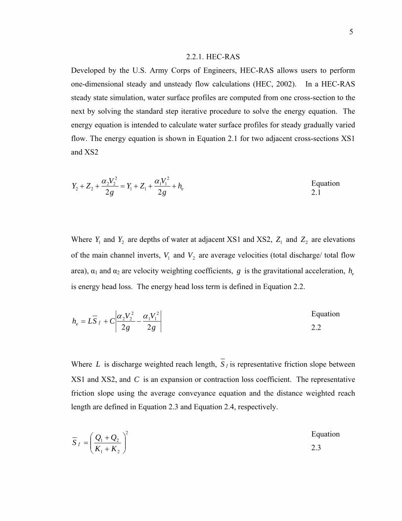
2.2.1. HEC-RAS

Developed by the U.S. Army Corps of Engineers, HEC-RAS allows users to perform

one-dimensional steady and unsteady flow calculations (HEC, 2002). In a HEC-RAS

steady state simulation, water surface profiles are computed from one cross-section to the

next by solving the standard step iterative procedure to solve the energy equation. The

energy equation is intended to calculate water surface profiles for steady gradually varied

flow. The energy equation is shown in Equation 2.1 for two adjacent cross-sections XS1

and XS2

ehgVZY

gVZY +++=++

22

211

11

222

22αα Equation

2.1

Where 1Y and 2Y are depths of water at adjacent XS1 and XS2, 1Z and 2Z are elevations

of the main channel inverts, 1V and 2V are average velocities (total discharge/ total flow

area), α1 and α2 are velocity weighting coefficients, g is the gravitational acceleration, eh

is energy head loss. The energy head loss term is defined in Equation 2.2.

gV

gV

CSLh fe 22

211

222 αα−+=

Equation

2.2

Where L is discharge weighted reach length, fS is representative friction slope between

XS1 and XS2, and C is an expansion or contraction loss coefficient. The representative

friction slope using the average conveyance equation and the distance weighted reach

length are defined in Equation 2.3 and Equation 2.4, respectively.

2

21

21⎟⎟⎠

⎞⎜⎜⎝

⎛++

=KKQQS f

Equation

2.3

6

robchlob

robrobchchloblob

QQQQLQLQL

L++

++=

Equation

2.4

Where K is conveyance, lobL , chL , and robL are cross-section reach lengths for flow in

the left over-bank, main channel, and right over-bank, respectively, and lobQ , chQ , and

robQ are arithmetic average of the flows between sections for the left over-bank, main

channel, and right over-bank, respectively.

To determine total conveyance and the velocity coefficient for a cross-section, HEC-RAS

subdivides flow in the main channel from the over-banks. Conveyance is calculated for

each subdivision using Equation 2.5 and Equation 2.6.

21

fKSQ = Equation

2.5

32486.1 AR

nK =

Equation

2.6

Where K is conveyance for the subdivision, n is Manning’s roughness coefficient for

the subdivision, A is flow area for the subdivision, and R is hydraulic radius for each

subdivision. The total conveyance for each subdivision is calculated as the sum of the

conveyance from the left over-bank, main channel, and right over-bank. Flow in the

main channel is subdivided only when the Manning’s roughness coefficient changes

within the channel area. The composite main channel Manning’s roughness coefficient is

defined in Equation 2.7.

7

( )3

2

1

5.1

⎥⎥⎥⎥

⎦

⎤

⎢⎢⎢⎢

⎣

⎡

=∑=

P

nPn

N

iii

c

Equation

2.7

Where cn is the composite or equivalent coefficient of roughness, P is the wetted

perimeter of the entire main channel, iP is the wetted perimeter of subdivision i, and in is

the coefficient of roughness for subdivision i.

Limitations in the HEC-RAS steady flow simulation include the assumptions that the

flow is steady, the flow is gradually varied, the flow is one-dimensional, and the river

channels have small slopes.

For situations when the flow may be rapidly varied, the momentum equation is used to

solve the water surface profiles. These situations include hydraulics of bridges, river

confluences, and mixed flow regimes such as hydraulic jumps. The momentum equation

used in HEC-RAS is shown in Equation 2.8.

111

11210

2122

2

22

22YA

gAQSLAALSAAYA

gAQ

f +=⎟⎠⎞

⎜⎝⎛ +

−⎟⎠⎞

⎜⎝⎛ +

++ββ

Equation

2.8

Where β is momentum coefficient that accounts for a varying velocity distribution in

irregular channels, 1Y and 2Y are depths measured from the water surface to the centroid

of the cross-sectional area at XS1 and XS2, 1Q and 2Q are discharge at locations XS1

and XS2, 1A and 2A are wetted area of the cross-section at locations XS1 and XS2, L is

distance between sections XS1 and XS2 along the channel, 0S is slope of the channel

based on mean bed elevations, and fS is slope of the energy grade line. Additional

information can be found in the HEC-RAS Hydraulic Reference Manual (HEC, 2002).

8

Required model parameters for HEC-RAS include topographic data in the form of a

series of cross-sections, a friction parameter in the form of Manning’s n values across

each cross-section, and flow data including flow rates, flow change locations, and

boundary conditions. For a steady state sub-critical simulation, the boundary condition is

a known downstream water surface elevation.

2.2.2. FESWMS

The depth-averaged Flow and Sediment Transport Model (FST2DH), part of the Federal

Highway Administration’s FESWMS, is a computer program that simulates movement of

water and non-cohesive sediment in rivers, estuaries, and coastal waters. FST2DH

applies the finite element method to solve steady or unsteady flow equations that describe

the two-dimensional depth averaged surface water flow (FESWMS, 2002). FST2DH is

used when vertical velocities are assumed to be negligible compared to lateral flow.

The finite element method is a numerical procedure for solving differential equations. In

this approach, continuous quantities are approximated by sets of variables at discrete

locations forming a network (mesh). FST2DH uses the Galerkin finite element method

to solve the governing differential equations discussed in the following paragraph.

The Galerkin finite element method begins by dividing a physical region into triangular

or quadrilateral elements. These elements are defined by nodes and vertices along their

boundary. Dependent variables are approximated within each element using values

previously defined at the node points of an element along with sets of interpolation

functions. In FST2DH, a mixed interpolation function is used in which quadratic

functions are used to interpolate unit flow rates at all nodes of an element and linear

interpolation is used to interpolate water depth at the vertices of an element. The mixed

interpolation function is used to stabilize the numerical solution. The method of

weighted residuals, a mathematical technique used for approximating solutions to partial

9

differential equations in which residuals to the solution are made to sum to zero, is

applied to the governing differential equations. More information on the Galerkin finite

element method and the method of weighted residuals can be found in the FESWMS

(2002).

The two-dimensional depth averaged flow equations used in FST2DH are described in

this section. Depth-averaged velocities in the horizontal x and y coordinate directions are

defined in Equation 2.9 and Equation 2.10, respectively.

∫=w

b

z

z

dzuH

U 1 Equation

2.9

∫=w

b

z

z

dzH

V v1 Equation

2.10

Where H is water depth, z is vertical direction, bz is bed elevation, wz is water surface

elevation, U is horizontal velocity in the x-direction at a point along the vertical

coordinate, V is horizontal velocity in the y-direction at a point along the vertical

coordinate.

Equations describing the depth-averaged surface water flow are found by integrating the

three-dimensional mass and momentum transport equations with respect to the vertical

coordinates from the bed to the water surface. In this approach, vertical velocities and

accelerations are assumed to be negligible. The vertically-integrated continuity equation

is shown in Equation 2.11.

mw q

yq

xq

tz

=∂∂

+∂∂

+∂∂ 21

Equation

2.11

10

Where UHq =1 is unit flow rate in the x direction, VHq =2 is unit flow rate in the y

direction, mq is mass inflow rate or outflow rate per unit area. Water mass density is

considered constant throughout the modeled region.

Equations describing momentum transport in the x and y directions are shown in

Equation 2.12 and Equation 2.13.

+Ω−∂∂

+∂∂

+⎟⎠

⎞⎜⎝

⎛∂∂

+⎟⎟⎠

⎞⎜⎜⎝

⎛+

∂∂

+∂∂

2212

211

21 q

xpH

xz

gHHqq

ygH

Hq

xtq ab

ρββ

Equation

2.12

( ) ( )01

=⎥⎦

⎤⎢⎣

⎡∂

∂−

∂∂

−−y

Hx

H xyxxsxbx

ττττ

ρ

+Ω−∂∂

+∂∂

+⎟⎠

⎞⎜⎝

⎛∂∂

+⎟⎟⎠

⎞⎜⎜⎝

⎛+

∂∂

+∂∂

1212

212

21 q

ypH

yz

gHHqq

xgH

Hq

ytq ab

ρββ

Equation

2.13

( ) ( )01

=⎥⎦

⎤⎢⎣

⎡∂

∂−

∂

∂−−+

yH

xH yyyx

syby

ττττ

ρ

Where β is isotropic momentum flux coefficient that accounts for the variation of

velocity in the vertical direction, ρ is water mass density, ap is atmospheric pressure at

the surface, Ω is the Coriolis parameter, τsx and τsy are surface shear stresses acting in the

x and y directions, respectively, and τxx, τxy, and τyy are shear stresses caused by

turbulence. More information regarding the governing equations used by FST2DH can

be found in the FESWMS (2002).

Required model parameters for FESWMS include topographic data in the form of a

continuous surface represented by a finite element mesh, a friction parameter for each

element in the form of a Manning’s n value, flow data, and a turbulent parameter. The

steady flow sub-critical simulation in FESWMS requires an upstream flow rate and a

downstream known water surface elevation. The only turbulent parameter in FESWMS

is the eddy viscosity. The eddy viscosity is further discussed in Section 2.5.

11

2.2.3. Case studies using 1D hydraulic models

Case studies have been performed using one-dimensional models to show the capabilities

of the model being used. Some of these case studies have been performed to calibrate

hydraulic models or validate results; but the main focus of these studies has been to

analyze the effect of topographic data on the hydraulic model. The effect of topographic

data on both one-dimensional and two-dimensional models will be further discussed in

Section 2.3. This section presents results from one-dimensional case studies.

Case studies using one-dimensional models such as HEC-RAS (Brandt, 2005; Omer,

2003; and Casas, 2006), HEC-2 (Mohammed, 2006), and HEC-6 (Sinnakaudan, 2002)

have been performed. In each of these studies, the goal has been to show how the effect

of changes in topography will impact the floodplain. A one-dimensional model is often

selected for this process because it represents the most basic approach to floodplain

modeling. In each of the three studies listed above, the one-dimensional model used was

successful in showing how a change in topography would affect the model. In the case

study of the Linggi River in Seremban Town, Malaysia, HEC-2 was used to calibrate and

validate the results. It was shown that the absolute error in predicted water surface levels

was within 5% of the observed levels (Mohammed, 2006).

2.2.4. Case studies using 2D hydraulic models

Case studies have been performed using two-dimensional models to show the capabilities

of the model being used. Some of these case studies have been performed to calibrate

hydraulic models or validate results while some have been performed to develop flood

maps of flood levels. This section presents discussion related to two-dimensional

models.

A study of a 4.6 mile reach of the Flint River at Albany, Georgia was performed using

FESWMS to develop incremental 1-ft flood surfaces corresponding to stream gages data.

In this study, the model was calibrated using a 120,000 cfs flow by adjusting the eddy

12

viscosity until the water surface elevation determined by the model matched the stream

gage (Musser and Dyer, 2005). Results show that the model was able to be validated

against a flow of 86,000 cfs.

In a similar study performed by the United States Geological Survey (USGS) on the Ohio

River, Jefferson County, Kentucky, calibration and validation of the two-dimensional

Resource Management Associates-2 (RMA-2) were explored (Wagner and Mueller,

2001). The model was calibrated at a low flow value (35,000 cfs) and validated with data

at a high flow (390,000 cfs). From the calibration and validation, it was determined that

the RMA-2 model was a good representation of the Ohio River below steady flow

discharges of approximately 400,000 cfs.

In another study designed to evaluate the capabilities of two-dimensional models on the

Lower Blue River in Kansas City, Missouri, FESWMS was selected to perform steady-

state flood flows for a hydraulically complex region of the river to determine the

estimated extent of flood inundation (Kelly and Rydlund, 2005). The FESWMS

simulations provided information as to the needed design of hydraulic structures and

produced flood inundation maps at 2-ft water level intervals. According to this study, the

flood inundation maps created represent a substantial increase in the capability of public

officials and residents to minimize flood deaths and damage in the flood plain of the

Lower Blue River.

2.2.5. Case studies comparing 1D and 2D hydraulic models

Recent research has been conducted on comparing one-dimensional models with two-

dimensional models, including using HEC-RAS, LISFLOOD-FP, a raster based model,

and TELEMAC-2D, a finite element model, on a 60 kilometer reach of the river Severn,

UK (Horritt and Bates, 2002). LISFLOOD-FP is a combined 1D-2D model solving 1D

continuity and momentum equations in the main channel and 2D continuity and

momentum equations in the floodplain and TELEMAC-2D solves the 2D shallow water

13

equations. In this study, it was shown that HEC-RAS and TELEMAC-2D are both

capable of being calibrated against discharge or inundated area while LISFLOOD-FP

must be calibrated against an independent inundated area to produce acceptable results.

Similarly, a study performed on a 25 kilometer reach of the Consumnes River in the

Sacramento Valley, California compared three models; Water-Surface PROfile

Computations (WSPRO), MIKE 11, and MIKE 21 on a 30 meter resolution DEM (Juza

and Barad, 2000). WSPRO is a 1D model similar to HEC-RAS, MIKE 11 is an

unsteady-looped 1D model based on the Saint-Venant equations, and MIKE 21 is a 2D

implicit finite difference scheme used for unsteady flows. The results show that there are

significant differences in water surface elevations between WSPRO and MIKE 11 due to

the fact that MIKE 11 can characterize exchanges between the floodplain and channels,

whereas WSPRO cannot. Results also indicate that the 2D model more accurately

represents flow in the floodplain due to both lateral and longitudinal movement of water.

In a similar study to compare one-dimensional models with two-dimensional models, a

study of the River Alzette north of Luxembourg City examined a HEC-RAS simulation

with a Regression and Elevation-based Flood Information eXtraction (REFIX) simulation

for a 2 meter resolution LiDAR DEM. Results indicate that the floodplain from the

HEC-RAS simulation was larger than from the REFIX simulation (Schumann et al.,

2007). Other studies have also shown similar results between one-dimensional and two-

dimensional models such as a case study of the 1983 Rudd Creek Mudflow in Utah

where water surface profiles were found to be similar between the one-dimensional HEC-

2 and the two-dimensional FLO-2D (O’Brien et al., 1993).

Similarly, a study of a 6 kilometer reach of the River Wharf, UK compared inundation

extent from HEC-RAS with a two-dimensional diffusion wave model (Tayefi et al.,

2007). The DEM for this study was created using a combination of 58 GPS surveyed

cross-sections for the main channel and remotely sensed LiDAR for the floodplains. The

results from this study show that, in qualitative terms, the two-dimensional model

14

produces the best results although the one-dimensional model could be calibrated to

produce accurate results.

Because of the increasing availability and popularity of two-dimensional flood inundation

models, studies have been performed to compare the performance of multiple 2D models.

In a study of three 2D models it was determined that use of a simplified 2D model would

give errors of approximately 10% while offering savings in computational effort

(Leopardi et al., 2002). The three models used in this case study were a complete two-

dimensional model, FIVFLOOD, and two simplified models, PA-31 and MCEP.

2.2.6. Combined 1D-2D hydraulic models

A recent trend in flood inundation modeling is the use of a combined one-dimensional

main channel model with a two-dimensional floodplain model. On a study of the Ticha

Orlice River confluence with the Trebovka River in the Central Czech Republic, a one-

dimensional floodplain model was compared with a hybrid one-dimensional two-

dimensional model. In this urban setting, it was found that the results of the Sobek 1D

and Sobek 1D-2D model were comparable, primarily as a result of the flood extent being

constrained by road and railway embankments (Werner et al., 2005). The DEM used in

this study was derived from LiDAR.

The use of a combined 1D-2D model was also used in a case study of the lower Mekong

River in Thailand (Dutta et al., 2007). The model consisted of the 1D unsteady dynamic

wave form of Saint Venant’s equation for river channel simulation combined with 2D

unsteady equations for floodplain flow. For this study, a 1 kilometer grid resolution was

used due to the large basin being considered. Results indicate that this model

demonstrated similar alignment with the observed data in terms of water level and

discharge as well as flood extent. It was inferred that this model is a reasonable approach

to predict both the magnitude and duration of flood events to a reasonable degree of

accuracy. Other studies have also shown that a combined 1D-2D model produce

15

acceptable results in flood inundation modeling (McMillan and Brasington, 2007; Tayefi

et al., 2007).

2.3. Effects of topography on hydraulic models

Due to the recent availability of high resolution elevation data such as LiDAR, it is

becoming possible to develop increasingly accurate floodplain maps. In some areas in

the United States as well as around the world, LiDAR elevation data, or similar resolution

elevation data, are available. From recent studies, it has been proven that topography is

one of the most important parameters in flood inundation modeling (Shuman et al., 2007;

Haile and Reintjes, 2005) This leads to the question of how much accuracy is gained in

floodplain mapping by using a higher resolution elevation dataset. The following section

describes some recent studies on the effect of topography on hydraulic models.

In a recent study of the Santa Clara River near the Castaic Junction in Southern

California, selected because of the availability of IfSAR (interferometric synthetic

aperture radar), NED and SRTM (shuttle radar topography mission) elevation data, it was

determined that the floodplain varies by at most 25%, with the NED 10 m dataset

predicting the smallest area and the SRTM-3 s dataset producing the largest area

(Sanders, 2007). The horizontal resolution of NED 10 m is approximately 10 meters,

while the horizontal resolution of SRTM-3 s is approximately 90 meters. In the same

study, an 8 kilometer reach of Buffalo Bayou near Houston, Texas was selected to

validate the results. This area is characterized by a relatively flat floodplain. Available

elevation datasets for this region were NED 3 m (LiDAR), NED 10 m, and NED 30 m.

For the 100-year storm event, floodplain area varied by only 5% and floodplain depth

varied by only 4% between the three NED terrains. Predictions for floodplain analysis

were performed using the two-dimensional BreZo model.

In a similar study performed on a 2 kilometer reach of the Ter River near Sant Julia de

Ramis, 5 kilometers downstream of Girona, Spain, seven digital terrain models (DTMs)

16

from three different sources were compared for flood inundation mapping using HEC-

RAS. The three sources for the DTMs were GPS survey including bathymetry, LiDAR,

and vectorial cartography from 5 meter contours. The results showed that flood

inundation area increased with decreasing DEM resolution (Casas et al., 2007).

In another study to further evaluate the impact of topography on hydraulic models, a

study, performed on a flood prone area drained by the Alzette River north of

Luxembourg City, involved the comparison of water stages derived from LiDAR, SRTM,

and topographic contours (Schumann et al., 2007). This study used the REFIX hydraulic

model to determine water stages. Results from this study indicate that the root mean

squared error (RMSE) of water surface elevations from LiDAR (2 meter spatial

resolution) was 0.35 meters, from the topographic contours was 0.7 meters, and from

SRTM (6 meter vertical precision) was 1.07 meters. The floodplain extent for the three

DEMs was then compared to a HEC-RAS simulation with LiDAR derived floodplains

and the Advanced Synthetic Aperture Radar (ASAR) observed flooded area. The

comparisons showed that the LiDAR derived flood maps agree 75% with the observed

flood, 73% with HEC-RAS, 62% with topographic contours, and 59% with SRTM.

The effect of topographic data is also examined in a study comparing the extent of flood

inundation on the River Nene, Northamptonshire, UK, using three remotely sensed

elevation datasets: LiDAR, stereo photogrammetry, and repeat-pass ERS interferometric

SAR (InSAR) (Wilson and Atkinson, 2003). Using the LISFLOOD-FP flood inundation

model, described in detail by Bates and De Roo (2000), the most accurate predictions

were obtained using the LiDAR data followed by the photogrammetric data when

compared to aerial photography.

2.3.1. DEM Resolution

The effects of re-sampling a DEM have also been studied. In an urban case study of the

city of Tegucigalpa, Honduras, a LiDAR derived DEM was re-sampled to a resolution of

17

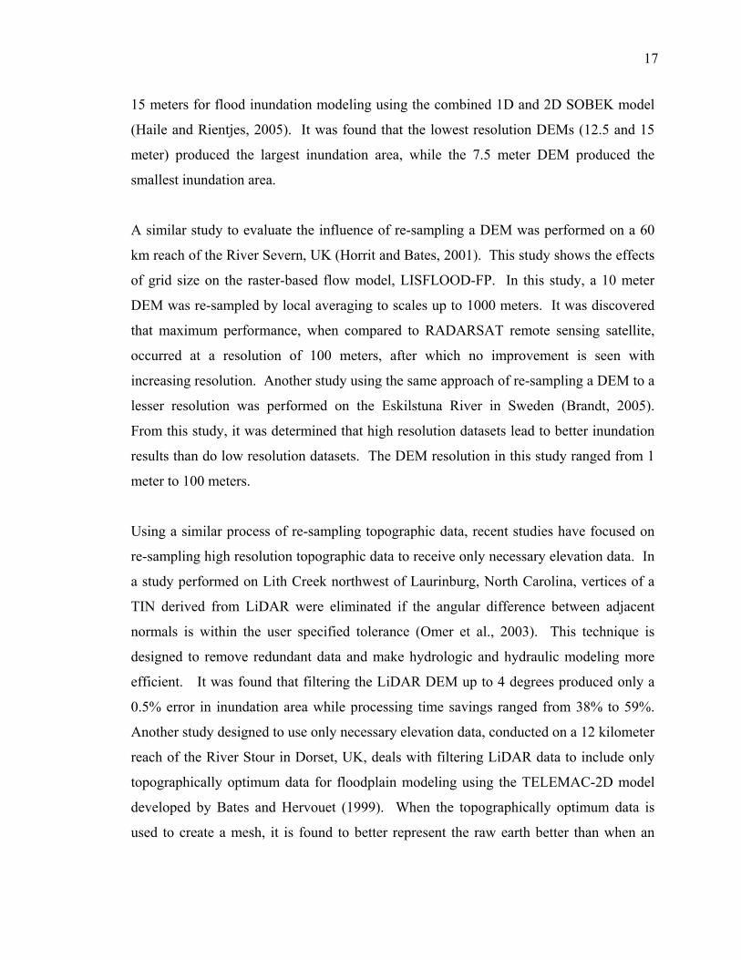
15 meters for flood inundation modeling using the combined 1D and 2D SOBEK model

(Haile and Rientjes, 2005). It was found that the lowest resolution DEMs (12.5 and 15

meter) produced the largest inundation area, while the 7.5 meter DEM produced the

smallest inundation area.

A similar study to evaluate the influence of re-sampling a DEM was performed on a 60

km reach of the River Severn, UK (Horrit and Bates, 2001). This study shows the effects

of grid size on the raster-based flow model, LISFLOOD-FP. In this study, a 10 meter

DEM was re-sampled by local averaging to scales up to 1000 meters. It was discovered

that maximum performance, when compared to RADARSAT remote sensing satellite,

occurred at a resolution of 100 meters, after which no improvement is seen with

increasing resolution. Another study using the same approach of re-sampling a DEM to a

lesser resolution was performed on the Eskilstuna River in Sweden (Brandt, 2005).

From this study, it was determined that high resolution datasets lead to better inundation

results than do low resolution datasets. The DEM resolution in this study ranged from 1

meter to 100 meters.

Using a similar process of re-sampling topographic data, recent studies have focused on

re-sampling high resolution topographic data to receive only necessary elevation data. In

a study performed on Lith Creek northwest of Laurinburg, North Carolina, vertices of a

TIN derived from LiDAR were eliminated if the angular difference between adjacent

normals is within the user specified tolerance (Omer et al., 2003). This technique is

designed to remove redundant data and make hydrologic and hydraulic modeling more

efficient. It was found that filtering the LiDAR DEM up to 4 degrees produced only a

0.5% error in inundation area while processing time savings ranged from 38% to 59%.

Another study designed to use only necessary elevation data, conducted on a 12 kilometer

reach of the River Stour in Dorset, UK, deals with filtering LiDAR data to include only

topographically optimum data for floodplain modeling using the TELEMAC-2D model

developed by Bates and Hervouet (1999). When the topographically optimum data is

used to create a mesh, it is found to better represent the raw earth better than when an

18

elevation dataset is applied to a mesh created independent of topography and the

differences are hydraulically significant (Bates et al., 2003).

2.3.2. DEM Accuracy

Other recent studies have focused on the accuracy of the DEM, not the accuracy of the

floodplain. These studies are performed to show the differences and errors in certain

DEMs, but are not applied to any hydraulic models. In a study of the Swift and Red Bud

Creek watersheds in North Carolina, DEMs were created from LiDAR, IfSAR, NED 10

m, and NED 30 m data to test the accuracy of the methods (Hodgson et al., 2003). The

root mean squared error (RMSE) for the LiDAR dataset was 93 cm, the lowest value of

the four DEMs tested. The RMSE for the NED-1/3 s DEM was 163 cm, for the NED-1 s

DEM was 743 cm, and for the IfSAR was 1067 cm. LiDAR and IfSAR data were

collected during leaf-on conditions meaning the vegetation could have a large impact on

the DEM. In a separate study of a LiDAR dataset obtained for a reach of the River

Coquet, Northumberlank, UK, it was shown that deep water and vegetation introduce

anomalies in the LiDAR generated surface when compared to surveyed points (Charlton

et al., 2003). It was determined that LiDAR generated cross-sections are incomplete

where there is deep water present and distorted where trees are present. This study

specifically examined river environments, and not the elevation of the floodplain.

2.4. Effects of geometry on hydraulic models

Hydraulic model geometry, cross-section for one-dimensional models and mesh

resolution for two-dimensional models, is also an important factor in floodplain mapping.

The following sections describe some recent studies detailing to effect of geometry on

hydraulic models. The effect of cross-sectional configuration on one-dimensional

hydraulic models is presented in Section 2.4.1 and the effect of mesh configuration on

two-dimensional models is presented in Section 2.4.2.

19

2.4.1. Effect of 1D geometry on hydraulic models

Cross-sectional resolution for one-dimensional hydraulic models is discussed in this

section. According to the HEC-RAS manual, every effort should be made to obtain

cross-sections that accurately represent the stream and floodplain geometry. Cross-

sections are required at a representative locations throughout a stream such as where

changes occur related to discharge, slope, shape, or roughness. Cross-sections are also

required before and after bridges or control structures. The HEC-RAS manual also states

that cross-sections spacing is a function of stream size, slope, and uniformity of the

channel. This means that large uniform rivers with a flat slope will require the least

number of cross-sections. According to another study, cross-sections should be surveyed

at sufficiently frequent locations to describe the hydraulic behavior of the channel with

acceptable precision but should be cost effective (Samuels, 1990). According to this

paper, cross-sections should be placed at model limits, either side of hydraulic structures,

sites of importance to the client, and at all flow or water surface elevation measurements.

Other guidelines for cross-section spacing are as follows in Equation 2.14 through

Equation 2.17.

B20Spacing ≈ Equation

2.14

sD2.0Spacing Maximum =

Equation

2.15

30Spacing Maximum L

=

Equation

2.16

ss

qd

ε

−

=10Spacing Minimum

Equation

2.17

Where B is the width of the water surface, D is the bank full depth, s is main channel

slope, L is the length scale of the physically important flood wave, q is the number of

decimal digits of precision, d is the digits of precision lost, and εs is the relative error on

20

the surface slope. The first equation is designed as a first estimate of cross-section

spacing. The cross-section spacing guidelines from this paper were designed for main

channel flow only. It is expected that linking the floodplains to the main channel will

result in different conclusions for cross-section spacing. Results from a one-dimensional

analysis of the Pari River in Malaysia suggest that more cross-sections at lesser intervals

will result in improved flood inundation (Sinnakaudan et al., 2002).

2.4.2. Effect of 2D geometry on hydraulic models

Mesh resolution has also been a topic that has been studied recently in two-dimensional

hydraulic models. In a study of a purely hypothetical example river with the hydraulic

model TELEMAC-2D, it was discovered that the effects of mesh resolution were at least

as important as typical calibration parameters and that model response to changes in

mesh resolution were highly complex (Hardy et al., 1998). It was also shown that as the

resolution of the mesh increases, the extent of inundation decreases. Increasing

inundation extent as a result of reduced resolution is a direct consequence of loss of

topographic information in the main channel.

To further show the effect of mesh resolution on a two dimensional model, a seven

kilometer reach of the River Thames, UK, was examined using a 2D finite volume

model. Results from this study show that the model shows greater sensitivity to mesh

resolution than to topographic sampling (Horritt et al., 2006). The sensitivity in mesh

resolution was determined to be caused by larger elements not being able to represent

some hydraulic features which occur at scales smaller than the element size and changes

in the representation of the domain boundary due to differing element sizes.

In some recent studies using two-dimensional models, the effect of decomposing the

mesh according to vegetation heights has been examined. Using LiDAR elevation data,

it is possible to separate ground hits from surface object hits. Ground hits are used to

construct a DEM and surface object hits are used to determine the heights of vegetation

21

or buildings (Mason et al., 2003). Vegetation height is then used as a friction parameter

and applied to each node in a two-dimensional mesh. The detailed process of the so-

called LiDAR segmentation can be found in Mason et al. (2003) and Cobby et al., (2003).

This technique, combined with steady state TELEMAC-2D finite element model, was

tested on a reach of the River Severn, UK, for a 50 year flood event which occurred in

1998. The results from this study show that the variable friction factor approach

produced a flood extent that agreed in most places with the observed data without

calibration, although the constant floodplain friction model also produced accurate results

(Mason et al., 2003). Another study, performed on the same study area, found

improvements in this procedure by decomposing the mesh to reflect floodplain vegetation

features having differing frictional properties from their surroundings (Cobby et al.,

2003). The simulated hydraulics using this approach gave a better representation of the

observed flood extent than the simpler approach of sampling vegetation friction factors

onto a mesh created independent of vegetation.

Other studies of mesh resolution have been performed to determine river pattern flows at

smaller scales. In a study of a 400 meter reach of the North Fork of the Feather River

near Belden, California, it was determined that reducing the element sizes in the vicinity

of obstructions and banks is crucial to modeling flow patterns created by topographic

features (Crowder and Diplas, 2000). This study was performed to determine the types of

topographic features which should be included in 2D model studies and to what extent

topographic features such as boulders can influence predicted flow conditions.

Individual obstructions were seen to influence flow patterns up to a distance of 6-8 times

the obstruction diameter.

2.5. Model Parameters

In one-dimensional models, the roughness parameter, Manning’s n value, is important to

the solution of the computed water surface profile, and can be use as a calibrating

parameter. The equations used by HEC-RAS to determine Manning’s n values are

22

discussed in Section 2.2.1. According to HEC (2002), the selection of an appropriate

value for Manning’s n is very significant to the accuracy of the computed water surface

profiles. The value of Manning’s n depends on a number of factors including surface

roughness, vegetation, channel irregularities, size and shape of the channel, seasonal

changes, temperature, and suspended material. From HEC (2002), the main channel

Manning’s n should be between 0.025 for a clean straight channel to 0.15 for very weedy

reaches with deep pools and heavy stands of timber or brush. The Manning’s n in the

floodplain should be between 0.025 and 0.20. Values of Manning’s n that have been

used in recent studies using one-dimensional models include between 0.026 and 0.065 in

the floodplains (Casas et al., 2006) and between 0.03 and 0.05 in the main channel and

between 0.06 and 0.10 in the floodplains (Horritt and Bates, 2002).

In two-dimensional hydraulic models, such as FESWMS, the eddy viscosity is used as a

representation of the turbulence parameters. According to FESWMS (2002), the eddy

viscosity in natural channels is related to the bed shear velocity and the depth of flow by

Equation 2.18.

HuVt ∗±= )3.06.0( Equation

2.18

Where Vt is eddy viscosity, u* is bed shear velocity, and H is depth.

The bed shear velocity can be related to the depth and slope of the channel by Equation

2.19 for uniform flow.

gHSU =∗ Equation

2.19

Where g is the gravitational constant and S is slope of the channel.

23

Also according to FESWMS (2002), the eddy viscosity coefficient usually affects the

solution much less than the roughness coefficient, although the eddy viscosity can be

used as a convergence parameter. Large values of eddy viscosity tend to enhance model

convergence. For uniform flow, larger values of eddy viscosity only affect the water

surface elevations near the downstream end of the channel. For locations where the flow

is constricted, the eddy viscosity will have a large impact on the upstream water surface

elevation.

Some typical values of eddy viscosity have been used in previous studies and are

presented in this section. According to Zanichelli, et al., (2004), for deep channels, eddy

viscosities between 2.4 and 14.4 m/s2 are acceptable. An eddy viscosity of14.4 m2/s

corresponds to an eddy viscosity of nearly 150 ft2/s in English units. Also according to

this paper, eddy viscosity depends on element size, current speed, and the dynamic nature

of the problem. Other studies have used eddy viscosities of 10 ft/s2 for flow under

bridges (Winters, 2000) and of 0.6 m2/s for shallow water flow (Papanicolaou and

Elhakeem, 2006).

The roughness parameter, Manning’s n value is also an important parameter that can be

used in calibrating the two-dimensional model. According to FESWMS (2002), even

comparatively small changes in Manning’s n can produce significant changes in the water

surface profile with larger values of Manning’s n producing higher water surface

elevations. According to Hardy et al., (1999), the floodplain friction value has a far

greater effect on the model when compared with channel friction. Values of Manning’s n

that have been used in recent studies include 0.025 for the main channel and between

0.056 and 0.111 in the floodplain (Hardy, et al.), between 0.02 and 0.04 in the main

channel and between 0.2 and 0.1 in the floodplain (Horritt and Bates, 2002), and between

0.045 and 0.065 in the main channel (Tayefi, et al., 2007).

24

2.6. Summary

In this chapter, comparison of one- and two-dimensional models have been made, the

effect of both topographic and geometric data on the model has been examined, and a

description of important model parameters has been presented. Much of the research that

has been presented in this section deals with floodplain mapping in Europe. In Europe,

many hydraulic modeling and flood inundation studies have been performed including

using high resolution topographic data, using two-dimensional models, and comparing

one- and two-dimensional models. In the United States, most of the hydraulic modeling

and flood inundation mapping is the responsibility of the FEMA DFIRM program. The

FEMA DFIRM uses a one-dimensional model to develop 100-year floodplain boundaries

for many areas in the United States. Case studies for specific rivers have also been

performed by the USGS using two-dimensional hydrodynamic models. In most studies,

only the results of the hydraulic modeling and flood inundation mapping procedure for

one river have been presented. This thesis adds to current research by presenting a

comparison between one- and two-dimensional models for two study areas in the United

States. The effect of model geometry and topography is also presented for both study

areas.

25

CHAPTER 3. STUDY AREA AND DATA

3.1. Introduction

This section gives an overview of the two study areas, Strouds Creek in North Carolina

and the Brazos River in Texas and the data that will be used to simulate the floodplain

using one- and two-dimensional hydrodynamic models. The four topographic datasets

used are LiDAR, NED 10 m, NED 30 m, and an integrated DEM. Presented in the

following sections are river geometry characteristics, cross section and bridge data, land

use classifications in terms of the Manning’s n value, and flow data at various river

stations. For Strouds Creek, data is provided by the North Carolina Floodplain Mapping

Program (NCFMP) while for the Brazos River, data is provided by Fort Bend County.

3.2. Description of Strouds Creek

Strouds Creek is a 4 mile long tributary of the Eno River in Orange County, North

Carolina. Strouds Creek has an average width of 30 feet, an average slope of 0.56%, and

is characterized by a relatively narrow floodplain with a v-shaped valley. The land use

description for the Strouds Creek main channel range from a Manning’s n value of 0.04

to 0.05. In the floodplains, the Manning’s n value ranges from a value of 0.1 to 0.2.

Figure 3.1 shows the location of Strouds Creek as well as the original cross-sectional

configuration with some cross sections labeled for reference.

26

0 0.5 10.25 Miles

Figure 3.1 Strouds Creek Study Area

3.2.1. Cross-section and Bridge Data

The original HEC-RAS project file for Strouds Creek is obtained from the NCFMP and

consists of data for 55 cross-sections, one culvert, and three bridges. The original cross-

sectional configuration is shown in Figure 3.1. The original 55 cross-sections have an

average width of 404 feet and average spacing between cross-sections is 396 feet.

1010

9.9

1504

2.9

2155

0.9

7437

.3

1636

.9

2047

0.2

27

The following section provides the characteristics of each of the three bridges and one

culvert located on the reach of Strouds Creek being evaluated. For all bridges, a drag

coefficient, Cd is given as 2.0 and pier shape, K as 1.25. A drag coefficient equal to 2.0

corresponds to square nose piers. A pier shape coefficient of K equal to 1.25 corresponds

to a square nose and tail.

HWY 57 Culvert – Located at station 18165.6 feet.

The HWY 57 culvert road is 45 feet long. The culvert is a combination of two box

shaped culverts with a span of 10 feet and a rise of 8 feet. The entrance loss coefficient

and exit loss coefficient are assumed to be 0.4 and 1.0, respectively.

Governor Road Bridge – Located at station 15021.4 feet

The Governor Burke Road Bridge is 23 feet wide and 30 feet long. The bridge has no

piers.

Miller Road Bridge – Located at station 9919.1 feet

The Miller Road Bridge is 30 feet wide and 80 feet long. The bridge consists of two

piers, each one foot wide.

St. Mary’s Road Bridge – Located at station 1475.3 feet

The St. Mary’s Road Bridge is 26 feet wide and 50 feet long. The bridge consists of one

pier four feet wide.

3.2.2. Flow Data

The flow data for the 100-year return period are obtained from the HEC-RAS project

provided by NCFMP. Table 3.1 presents the steady state flow rates assigned at various

river stations.

28

Table 3.1 Flow Rates for Strouds Creek

Station (ft) Flow Rate (cfs)

21,550.9 1,427

20,470.2 1,759

15,042.9 2,288

10,109.9 2,964

7,437.3 3,592

1,636.9 3,629

3.3. Description of the Brazos River

The study area along the Brazos River is a 39.2 mile long stretch located in Fort Bend

County, Texas. The Brazos River is characterized by meandering bends and a relatively

flat floodplain with levees located on both sides of the river. The average width for the

Brazos River reach is around 500 feet and the average slope is 0.016%. The land use

classifications for the main channel range from a Manning’s n value of 0.035 to 0.042. In

the floodplains, the Manning’s n values range from 0.06 to 0.12. Figure 3.2 shows the

location of the Brazos River as well as the original cross-sectional configuration with

some cross section station numbers shown for reference.

29

0 4 82 Miles

Figure 3.2 Brazos River Study Area

3.3.1. Cross-section and Bridge Data

The original HEC-RAS project file for the Brazos River is obtained from Fort Bend

County and consists of data for 53 cross-sections and seven bridges. The original cross-

sectional configuration is shown in Figure 3.2. The original 53 cross-sections have an

average width of 26,577 feet and average spacing between cross-sections is 3,874 feet.

1582.25

1033

89.7

1588

28.9

2066

97.9

6680

5.17

13670.26

30

The following section provides the characteristics of each of the seven bridges located on

the reach of the Brazos River being evaluated. For all bridges a drag coefficient, Cd is

given as 1.2 and the pier shape coefficient, K as 1.25. A pier shape coefficient of K equal

to 1.25 corresponds to a square nose and tail.

FM 723 – Located at station 187388.2 feet.

The FM 723 Bridge Road is 690 feet long and 30 feet wide. The bridge consists of six

piers, each 2.5 feet wide.

ASTF Railroad – Located at station 144310.5 feet.

The ASTF Railroad Bridge Road is 900 feet long and 26.9 feet wide. The bridge consists

of 4 piers, each 9 feet wide.

SH 90A Southbound – Located at station 143739.9 feet.

The SH 90A Southbound Bridge Road is 990 feet long and 31 feet wide. The bridge

consists of 10 piers, the first seven of which are 2.5 feet wide while the remaining three

are each 3 feet wide.

SH 90A Northbound – Located at station 143432.3 feet.

The SH 90A Northbound Bridge Road is 1090 feet long and 44 feet wide. The bridge

consists of 9 piers, the first seven of which are 2.5 feet wide while the remaining two are

each 5.4 feet wide.

SH 99 – Located at station 105636.0 feet.

The SH99 Bridge Road is 1220 feet long and 73 feet wide. The bridge consists of 8

piers, each 5 feet wide.

SH 59 – Located at station 98377.74 feet.

The SH 59 Bridge Road is 1490 feet long and 180 feet wide. The bridge consists of 9

piers, each of which is 3 feet wide.

31

ATSF Railroad – Located at station 24353.22 feet.

The ATSF Railroad Bridge is 750 feet long and 185 feet wide. The bridge consists of 6

piers, the first has a width of 2.7 feet, the second has a width of 7.4 feet, while the

remaining four piers each have a width of 8.5 feet.

3.3.2. Flow Data

The flow data for the 100-year return period are obtained from the HEC-RAS project

provided by Fort Bend County. Table 3.1 presents the steady state flow rates assigned at

various river stations.

For the 100-year flow, Table 3.2 presents the steady state flow rates assigned at various

river stations. A downstream water surface elevation of 57.37 feet was given in the

original HEC-RAS project file.

Table 3.2 Flow Rates for Brazos River

Station (ft) Flow Rate (cfs)

206,697.9 167,000

143,373.8 164,000

1,582.3 158,000

3.4. Light Detection and Ranging Elevation Data

LiDAR (light detection and ranging) data for North Carolina is available from NCFMP

and for Texas is available from Fort Bend County. LiDAR data is collected from an

aircraft fitted with a laser which measures its distance to the ground, and by tracking the

position, pitch and roll of the aircraft the coordinates of the ground surface can be

calculated. The laser works with pulses of light that reflect from the earth back to the

aircraft. If the pulse reflects off multiple sources, such as vegetation and bare earth, it is

common to use the first reflecting pulse as the elevation of vegetation, and the last

32

reflecting pulse as the elevation of the bare earth (Sanders, 2007). LiDAR data for North

Carolina and Texas is characterized by a vertical accuracy of approximately 0.25 meters.

3.5. National Elevation Dataset

National Elevation Dataset (NED) is available for North Carolina, Texas and throughout

the contiguous United States from www.seamless.usgs.gov. The NED 30 m DEM is

characterized by a horizontal resolution of approximately 30 meters and a vertical

accuracy of 7 - 15 meters. The NED 10 m DEM is characterized by a horizontal

resolution of approximately 10 meters and a vertical accuracy of approximately 7 meters.

NED is a combination of topographic data from several sources including LiDAR and

United States Geological Survey (USGS) quadrangle maps (Sanders, 2007). The vertical

accuracy of NED is provided by the USGS.

3.6. Integrated Dataset

Because LiDAR or NED does not contain main channel bathymetry, the surveyed cross-

section data are integrated with LiDAR to create a new topographic dataset. A detailed

description of the process used in creating the integrated DEM is described in Merwade

(2007). The integrated DEM is expected produce a more accurate representation of the

main channel. The integrated DEM has the same resolution as the LiDAR dataset in the

floodplain.

33

CHAPTER 4. METHODOLOGY

4.1. Introduction

This chapter provides a detailed methodology for creating flood inundation maps using

HEC-RAS and FESWMS for Strouds Creek and the Brazos River. For Strouds Creek, 18

cross-sectional modifications and two mesh resolutions are evaluated for four DEMs:

integrated, LiDAR, NED 10 m, and NED 30 m resulting in 72 HEC-RAS project files

and 8 SMS project files. For the Brazos River, 12 cross-sectional configurations and two

mesh resolutions are evaluated for each of the four DEMs resulting in 48 HEC-RAS

project files and 8 FESWMS project files. Flow simulation data are taken from the

original HEC-RAS project file. For the HEC-RAS simulations, the same process is used

for both Strouds Creek and the Brazos River to generate the floodplain. For the

FESWMS simulations, the process used to generate the floodplain for Strouds Creek is

modified for the Brazos River to accommodate the larger area and to take into account

the locations of the levees. A tutorial for using SMS is included in the appendix as a CD-

ROM.

4.2. 1D floodplain mapping using HEC-RAS

The original HEC-RAS project data is imported to ArcGIS using HEC-GeoRAS,

(available from the website http://www.hec.usace.army.mil/SOFTWARE/hec-ras/hec-

georas.html) an ArcGIS extension that provides the user with a set of procedures, tools,

and utilities for the preparation of GIS data for input to HEC-RAS and generation of GIS

data from HEC-RAS output. The data imported by HEC-GeoRAS consists of a river

centerline and cross-sections. Using the HEC-GeoRAS toolbar, bank lines and flow

paths are digitized by overlaying an aerial photograph on the data. Bridges and culverts

34

are then digitized using the aerial photograph as well as the cross-sections as a spatial

reference. In HEC-RAS, it is common practice to place cross-sections on either side of

bridges or other hydraulic structures. Bridges are placed between these binding cross-

sections. Ineffective flow areas, defined as any area that contains water that has zero

velocity, and flow obstructions, defined as any area that has no water and no flow, are

digitized by referencing the aerial photograph (Merwade, 2006).

To complete the representation of the HEC-RAS project file in ArcGIS, in addition to

geometry data such as cross-sections, river centerline, bridges, and left and right banks,

HEC-RAS requires Manning’s n values and levee locations. The distribution of

Manning’s n values in the original HEC-RAS project file is used to create a land use

polygon in ArcGIS. Similarly, the locations of the levees in the HEC-RAS file are

referenced, along with an aerial photograph, to create levees in ArcGIS. Figure 4.1

shows the ArcGIS shape files necessary for a HEC-RAS analysis.

Figure 4.1 HEC-GeoRAS configuration for a) Strouds Creek b) Brazos River

Once the project is set up, different HEC-RAS cross-sectional configurations using the

four different topographic datasets are created to show how different cross-sectional

configuration and topographic data will affect the resulting floodplain. For Strouds

Creek, 18 cross-sectional configurations are analyzed, while for the Brazos River, 12

cross-sectional configurations are analyzed. The cross-sectional modifications for

a) b)

35

Strouds Creek and the Brazos River are discussed in sections 4.2.1 and 4.2.2,

respectively.

4.2.1. Strouds Creek Cross-sectional Modifications

Table 4.1 provides information for each of the cross-sectional modifications for Strouds

Creek. For all cross-sectional modifications, cross-sections on either side of a bridge or

culvert and cross-sections that are a flow change location in the original HEC-RAS

project file are not removed. The exception to this is the SR3 modification where the

cross-sections immediately upstream and downstream of the culverts are removed. For

any cross-sectional modification where cross-sections are added, if the original cross-

sections are already close together, no cross-sections are added in between the cross-

section. In Table 4.1, S represents the original Strouds Creek cross-sections, while any

modification with SA shows cross-sections are added, any modification with SR shows

cross-sections are removed, and any modification with SI shows cross-sections are

located at a specific interval.

36

Table 4.1 Description of the Cross-sectional Configurations for Strouds Creek

Cross-section Code Description # of Cross-sections

S Original Cross-sections 55

SA1 Double Cross-sections 97

SA2 Triple Cross-sections 139

SA3 Every Curve 76

SR1 Half Cross-sections 34

SR2 One-Third Cross-sections 25

SR3 Without Culvert 53

SR4 Without Cross-section 2 54







SR11 Without Cross-section 41-43 52

SI1 250 ft Interval 94



Shown in Figure 4.2 are the locations of cross-sections removed for cross-sectional

modifications SR3 to SR11.

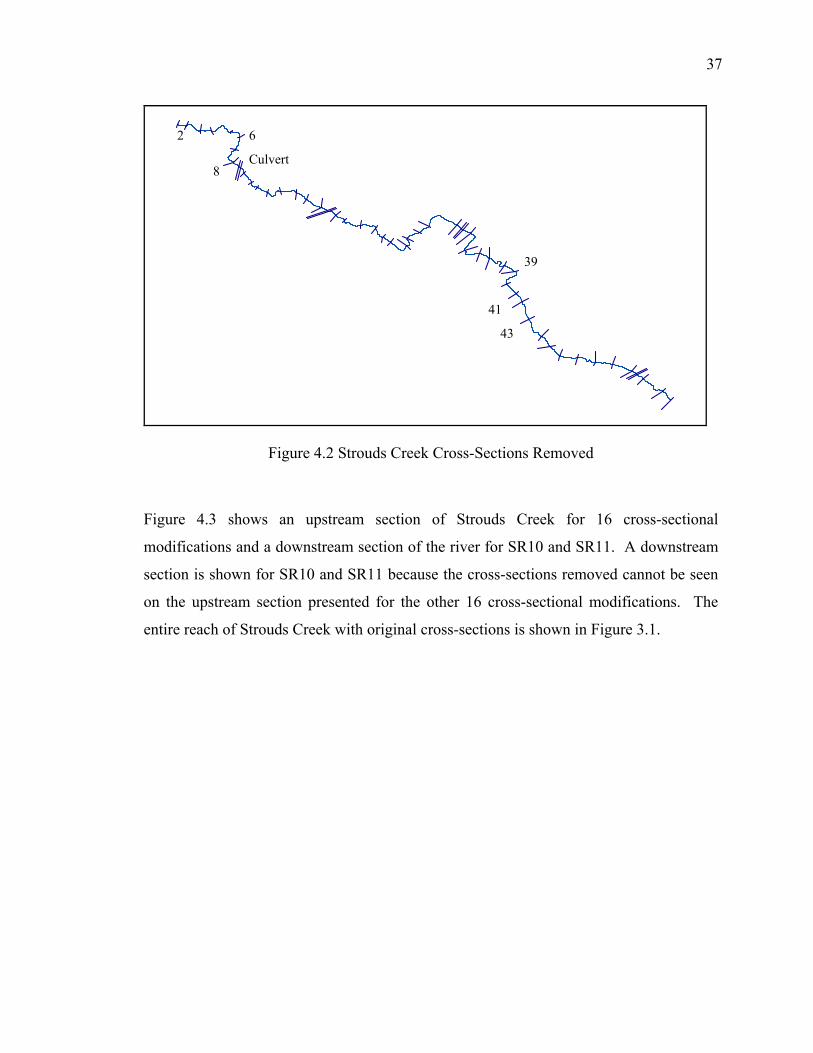
37

Figure 4.2 Strouds Creek Cross-Sections Removed

Figure 4.3 shows an upstream section of Strouds Creek for 16 cross-sectional

modifications and a downstream section of the river for SR10 and SR11. A downstream

section is shown for SR10 and SR11 because the cross-sections removed cannot be seen

on the upstream section presented for the other 16 cross-sectional modifications. The

entire reach of Strouds Creek with original cross-sections is shown in Figure 3.1.

2 6

8

39

41

43

Culvert

38

Figure 4.3 Strouds Creek Cross-Sectional Configuration

4.2.2. Brazos River Cross-sectional Modification

Table 4.2 provides information for each of the cross-sectional modifications for the

Brazos River. For all cross-sectional modifications, cross-sections on either side of a

bridge or culvert and cross-sections that are a flow change location in the original HEC-

RAS project file were not removed. For any cross-sectional modification where cross-

sections are added, if the original cross-sections are already close together, no cross-

sections are added in between the cross-section. In Table 4.2, B represents the original

S SA1 SA2

SA3 SR1 SR2

SR3 SR4

SR6 SR7 SR8

SR5

SI1) SI2

SI3

SR9

SR11 SR10

39

Brazos River cross-sections, while any modification with BA shows cross-sections are

added and any modification with BR shows cross-sections are removed.

Table 4.2 Description of the Cross-sectional Configurations for the Brazos River

Cross-section Code Description # of Cross-sections

B Original Cross-sections 53

BA1 Double Cross-sections 84

BA2 Triple Cross-sections 106

BA3 Every Curve 61

BR1 Half Cross-sections 34

BR2 One-Third Cross-sections 28

BR3 Without Cross-section 2 52

BR4 Without Cross-section 8-9 51



BR7 Without Cross-section 40 52


Shown in Figure 4.4 are the locations of cross-sections removed for cross-sectional

modifications BR3 to BR8.

40

Figure 4.4 Brazos River Cross-Sections Removed

Figure 4.5 shows an upstream section of the Brazos River for nine cross-sectional

modifications and a downstream section for cross-sectional modifications BR6, BR7, and

BR8. A downstream section is shown for BR6, BR7, and BR8 because the cross-sections

removed cannot be shown on the upstream section presented for the other nine

modifications. The entire reach of the Brazos River with original cross-sections is shown

in Figure 3.2.

2

22

9

36 40

50

41

Figure 4.5 Brazos River Cross-Sectional Configuration

4.2.3. Topographic Representation

Each of the cross-sectional modifications are then applied to each of the four digital

elevation models (DEM); integrated, LiDAR, NED 10 m, and NED 30 m using the HEC-

GeoRAS extension. The HEC-GeoRAS extension assigns elevation data to all shape

files created in ArcGIS. To assign elevation data to the levee shape file, the elevations of

the levee points are interpolated along the length of the levee to assign elevations at all

locations between points. With elevations assigned to each shape file, the information is

exported to HEC-RAS for a steady state analysis. For Strouds Creek, 18 HEC-RAS

project files are created and for each of the four DEMs and for the Brazos River, 12

HEC-RAS project files are created for each DEM.

BA2 B BA1

BR2 BA3 BR1

BR5 BR3 BR4

BR6 BR8 BR7

42

4.2.4. Flow Data and Simulation

In HEC-RAS, information must be provided for bridge deck/roadway, bridge piers, and

bridge modeling approach. This information is copied from the original HEC-RAS

project file. To reduce the number of points along each cross-section to an acceptable

level, each cross-section is filtered to 500 points. Flow data available from the original

HEC-RAS project is used as input for steady state analysis. Included in the flow data are

flow change locations, flow rates, and boundary conditions. Steady state simulation

results in HEC-RAS are exported to ArcGIS for preparing flood inundation maps using

HEC-GeoRAS.

4.2.5. Flood Inundation Mapping

HEC-GeoRAS is used to create the boundary of the flood extent and the depth of water at

each location within the boundary. HEC-GeoRAS creates water depths and floodplain

boundaries by subtracting topographic data from water surface elevations imported from

HEC-RAS. An area where the water depth is greater than zero is considered to be in the

flood boundary. To analyze the data, two variables are taken into consideration. The

first being the area of the flood extent and the second being the width of flood along each

cross-section in the original HEC-RAS project file. A Visual Basic for Applications

(VBA) macro is created to extract the width of the floodplain and these results are

compared to results for different digital elevation models, different cross-sectional

configurations, as well as the results from the two-dimensional analysis.

4.3. 2D floodplain mapping using FESWMS for Strouds Creek

Surface-water Modeling System (SMS) is a pre and post processor for a suite of two-

dimensional finite element and finite difference mesh models. For this study, FESWMS

is used as the finite element model to simulate flow conditions for Strouds Creek for the

same discharges, land use classifications, and bridge data used in the HEC-RAS

simulations.

43

To create the two-dimensional mesh, the land use shape file created in ArcGIS is opened

in the GIS module of SMS. Using the GIS module, the land use shape file is converted to

a feature object for use in the Map module of SMS. In the map module, polygons are

created for each land use classification based on a Manning’s n value. One of the goals

when creating the mesh is to create uniform mesh elements. To do this, most of the

Manning’s n value polygons are subdivided. For most polygons, the patch meshing type

is selected. The patch meshing type provides rectangular elements which are semi-

uniform. One of the requirements for the patch meshing type is a polygon with exactly

four nodes. For any polygons with only three nodes, a paving meshing type is selected.

The paving meshing type generally creates triangular elements. Material type, or

Manning’s n value, is also assigned in the map module. With the material type and

meshing type selected, the map is converted to a mesh.

4.3.1. Strouds Creek Mesh Resolution

For each of the four digital elevation models, a map with vertices at 10 feet intervals and

a map with vertices at 20 foot intervals are created. Figure 4.6 shows the 10 foot and 20

foot mesh resolutions for a section of Strouds Creek.

Figure 4.6 Strouds Creek mesh resolution in SMS a) 10 foot b) 20 foot

a) b)

44


The next step in the two-dimensional floodplain mapping process involves using ArcGIS

to convert the DEMs into an acceptable file type for use in SMS. The DEMs are

converted into ASCII (American Standard Code for Information Interchange) format

using Arc Toolbox in ArcGIS. The ASCII format is recognized by SMS whereas the

raster or TIN format used in GIS is not recognized by SMS. The ASCII file is opened in

the Scatter Module of SMS. The resulting scatter set will provide (x,y,z) data for all the

elevation points in a given elevation dataset. This process is followed for each of the

topographic datasets considered. In the scatter module, the ASCII elevation file is

linearly interpolated to assign an elevation to each node in the mesh.


In the mesh module, material properties, including an eddy viscosity of 5 ft2/s are

assigned. According to FESWMS (2002), increasing the eddy viscosity causes velocity

gradients to be reduced increasing the chance of a successful simulation. According to a

USGS study of the Flint River at Albany, Georgia, eddy viscosity can be used as an

important parameter in calibrating the model to obtain correct water surface elevations.

Using Equation 2.18 and Equation 2.19, the eddy viscosity for Strouds Creek should be

in the range of 5 ft2/s for a water depth ranging between 5 and 12 feet and an average

channel slope of 0.56%. Also in the mesh module, an upstream flow rate and a

downstream water surface elevation are assigned. Because the Strouds Creek HEC-RAS

project file has six different flow rates at different sections along the reach being

considered, the land use file was divided into six separate meshes. Flow rates in SMS are

assigned according to Table 3.1, which shows the flow rates given in the HEC-RAS

project file, and the flow change locations are shown in Figure 3.1. Each mesh is then

subdivided to improve the chances of a successful FESWMS simulation and to reduce the

time for each simulation. The downstream water surface elevation for the entire reach of

Strouds Creek being studied is given in the HEC-RAS project file to be 478.64 feet.

FEWSMS spin down is used to determine the final solution for the given boundary

45

conditions. When using FESWMS, an initial condition must be specified such that all

nodes in the mesh are initially wet. With the user specified initial conditions, FESWMS

spin down incrementally decreases the downstream water surface elevation until the

specified boundary condition is reached. When the most downstream mesh section

successfully converged to a steady state solution for this water elevation, the upstream

water surface elevation of this section is recorded and used as the downstream water

surface elevation boundary condition for the next section upstream. This process is

repeated for each section. Due to trouble with model convergence on the section which

contained the culvert, SMS results only consider the portion of Strouds Creek

downstream of the culvert. When SMS cannot successfully spin down the water surface

elevation to the desired value, the model has not converged for the given parameters.


To determine the width of the floodplain at specified cross-sections to compare with the

results from the one-dimensional HEC-RAS simulation, the floodplain results from SMS

are exported for use in ArcGIS. To do this, a contour of zero water surface elevations

was created in the mesh module. This contour, when converted to the map module,

represented the boundary of the floodplain. The contour was then saved as a shape file

and opened in ArcGIS. In ArcGIS, the shape files for each section were merged to create

a floodplain for the entire length of Strouds Creek. A VBA macro was created to extract

the width of the floodplain at original HEC-RAS cross-section locations, and these results

are compared with results for different digital elevation models, different mesh spacing,

as well as the results from the one-dimensional analysis.

4.4. 2D floodplain mapping using FESWMS for the Brazos River

The process to complete the two-dimensional analysis of the floodplain for the Brazos

River is intended to be similar to that done for Strouds Creek, but due to the large area of

the floodplain and locations of the levees, only a nine mile long upstream section of the

46

river is analyzed with FESWMS. The entire reach could not be analyzed at an acceptable

mesh resolution because the number of mesh elements produced is too large for the

computing capabilities of the computer used in this study. The nine mile section of the

river is selected such that the mesh resolution would be refined enough to accurately

model the flow through the compound channel and no levees are split in that section.

The levees, as a general trend, run parallel to the river before branching off perpendicular

to the river. If the levees are split and modeled in SMS, the resulting floodplain will

always show flow on both side of the levees because there is no upstream levee boundary

keeping the flow from the floodplains.

Instead of using the GIS land use shape file to create the basis for the mesh to be used in

SMS, a scatter file created from the elevation ASCII file is used. In this study for the

Brazos River, a 500 foot interval is selected because of the large area of the floodplain.

The 500 foot spacing scatter file is then converted to a mesh. The advantage of using this

technique is that an ideal mesh is created. Each mesh element created is either a perfect

square or a right triangle. In the vicinity of the main channel, the mesh is refined to

create elements with mesh spacing less than 500 feet. The Brazos River main channel is

deep and when the mesh is not refined in the vicinity of the main channel, important

elevation data is lost within the main channel. If the mesh is not refined in the main

channel, the flow through the main channel will decrease causing more flow to be routed

through the floodplains and will produce unrealistic results for floodplain analysis. After

creating the mesh, land use Manning’s n values are assigned. Manning’s n values are

assigned as either floodplain or main channel. Floodplain zones are assigned a

Manning’s n value of 0.12 while the main channel is assigned a Manning’s n value of

0.05. The Manning’s n values selected are representative values given in the HEC-RAS

project file.

47

4.4.1. Brazos River Mesh Resolution

For each of the four digital elevation models, maps with main channel vertices at 125 and

250 foot intervals are created. Figure 4.7 shows the 125 and 250 foot main channel mesh

resolution for the nine mile section of the Brazos River being considered.

Figure 4.7 Brazos River mesh resolution in SMS a) 125 foot b) 250 foot


The next step in the two-dimensional floodplain mapping process involves assigning

elevation data to the mesh. The process is the same as what is done for Strouds Creek

and can be seen in Section 4.3.2.


With the mesh created, a steady state solution was selected and all material properties and

turbulence parameters were assigned. An eddy viscosity of 200 ft2/s is selected because

this value allowed for model convergence for each of the four topographic datasets for

both the mesh resolutions considered. Using Equation 2.18 and Equation 2.19, the eddy

viscosity for the Brazos River should be between 10 and 30 ft2/s. For the integrated

DEM, the model will converge for an eddy viscosity of 25 ft2/s, but for the lower

resolution DEMs, the model does not converge for an eddy viscosity lower than 200 ft2/s.

a) b)

48

According to FESWMS (2002), large increases in eddy viscosity raise upstream water

surface elevations far less than large increases in roughness coefficients for a channel of

uniform width, but do reduce velocity gradients increasing the chance for a successful

simulation. According to a study performed by Zanichelli et al. (2004), eddy viscosities

of close to 150 ft2/s are acceptable for deep channels. To be consistent between each

topographic dataset, the value of eddy viscosity is selected such that each topographic

dataset can achieve model convergence. An upstream flow rate and downstream water

surface elevation boundary conditions are assigned, and FEWSMS spin down is used to

converge to a successful simulation. For this section of the Brazos River, the

downstream water surface is determined to be 86.97 feet using the HEC-RAS project file.

The flow rate, also given in the HEC-RAS project file, is 167,000 cfs.


To determine the width of the floodplain at specified cross-sections to compare with the

results from the one-dimensional HEC-RAS simulation, the same process is used as that

described for Strouds Creek in Section 4.3.4.

49

CHAPTER 5. RESULTS

5.1. Introduction

The results from steady flow hydraulic modeling and flood inundation mapping are

presented in this chapter for both Strouds Creek and the Brazos River. For both rivers,

inundation area, average width of inundation along the original cross-sections, and

percent change in area using the integrated DEM as the benchmark are presented for each

DEM. To compare the effect of geometry on the one-dimensional model, 18 cross-

sectional configurations for Strouds Creek and 12 cross-sectional configurations for the

Brazos River are evaluated by determining area of inundation and average inundation

width along the original cross-sections for each DEM. To compare the effect of

geometry on the two-dimensional model, mesh resolutions of 10 and 20 feet for Strouds

Creek and 125 and 250 feet for the Brazos River are evaluated for each DEM by

determining inundation area and average width of inundation. The results from the HEC-

RAS and FESWMS simulations are then compared.

5.2. Effect of Topography on one-dimensional hydraulic model

In this section, four DEMs are evaluated for hydraulic modeling and floodplain mapping

using the original 55 HEC-RAS cross-sections for Strouds Creek and the original 53

cross-sections for the Brazos River. The extent of inundation is measured by the area of

inundation and the average width of inundation along the original cross-sections.

5.2.1. Strouds Creek

Table 5.1 presents the inundation area, the average width of inundation along the cross-

sections, and the percent change in inundation area using the results from the integrated

50

DEM as the benchmark. The percent change in inundation area is shown in parenthesis

for each DEM evaluated.

Table 5.1 Inundation for Original Cross-sections NED 30 m NED 10 m LiDAR Integrated

Area (mi2) (% change) 0.199 (64.35) 0.178 (46.67) 0.145 (19.87) 0.121 (0.00)Average Width (ft) 297.33 264.29 234.40 185.46

The results of this table show that the integrated DEM produces the least amount of

inundation area and the least average width of inundation, followed by the LiDAR, NED

10 m and NED 30 m DEMs. Overall, the area of inundation increases with decreasing

DEM resolution. Both the integrated and LiDAR DEMs have the same resolution data in

the floodplain, while the integrated DEM is a more accurate representation of the

topography in the main channel. The NED 10 m DEM has a horizontal resolution of

approximately 30 feet and the NED 30 m DEM has a horizontal resolution of

approximately 90 feet. The percentage increase in area is 64.35 % for the NED 30 m

DEM when compared to the integrated DEM.

Figure 5.1 further shows the difference in inundation area for each of the four DEMs

being considered. Figure 5.1 shows a magnified image of the floodplain developed using

the original cross-sections and each DEM.

51

LegendIntegrated

LiDAR

NED 10 m

NED 30 m

Figure 5.1 Inundation Boundary for a) Entire Reach; b) Magnified to a Bend in the River

The inundation extent for the integrated DEM shows that there are two areas, one near

the upstream section of the reach and one near the midpoint of the reach, where no

flooding is shown to take place. The area where no flooding is shown to take place near

the midpoint of the reach is magnified in Figure 5.1. For the LiDAR DEM, the upstream

area where no flooding occurred using the integrated DEM is now flooded, whiles the

area near the midpoint of the reach remains without flooding. For both the NED 10 m

DEM and NED 30 m DEM, both areas shown previously to have no flooding are now

flooded. In looking at the NED 30 m DEM, there is a clear change in resolution, with

the floodplain appearing as a series of large blocks.

a)

b)

52

The horizontal resolution for both the integrated DEM and the LiDAR DEM are the same

in the floodplain meaning a change in inundated area is due to a change in the

representation of the main channel. This change can be seen through a representative

HEC-RAS cross-section station 7986.1 feet for both the integrated and LiDAR DEMs

shown in Figure 5.2. The shape of the cross-sections are nearly identical, with the

exception being that the main channel for the integrated DEM is deeper than that of the

LiDAR DEM. Because LiDAR cannot penetrate deep water, in the LiDAR DEM cross-

section, the main channel invert is around 515 feet while the integrated DEM cross-

section has a main channel invert below 510 feet. As a result, the area of the main

channel is larger for the integrated DEM which means more flow is routed through the

main channel and less will flow in the floodplains. When less flow is routed through the

floodplains, the area of inundation is less. The difference in inundation extent can also be

seen in the fact that the water surface elevation for the LiDAR cross-section is higher

than that of the integrated DEM cross-section. The water surface elevations are 520.28

and 521.23 feet for the integrated and LiDAR DEMs.

0 100 200 300 400 500 600 700508

510

512

514

516

518

520

522

524

526

Station (f t)

Elev

atio

n (ft

)

Legend

WS 100-year

Ground

Bank Sta

0 100 200 300 400 500 600 700514

516

518

520

522

524

526

Station (f t)

Elev

atio

n (ft

)

Legend

WS 100-year

Ground

Bank Sta

Figure 5.2 Cross-section Station 7986.1 for the a) Integrated; b) LiDAR DEM

When the resolution is further decreased, as is the case for the NED 30 m DEM and the

NED 10 m DEM, the main channel definition is further reduced, and the extent of

inundation becomes larger. The width of the main channel of Strouds Creek is

approximately 30 feet, meaning when the resolution of the DEM exceeds 30 feet, each

cross-section sampled will have no more than one point located in the main channel. In

a) b)

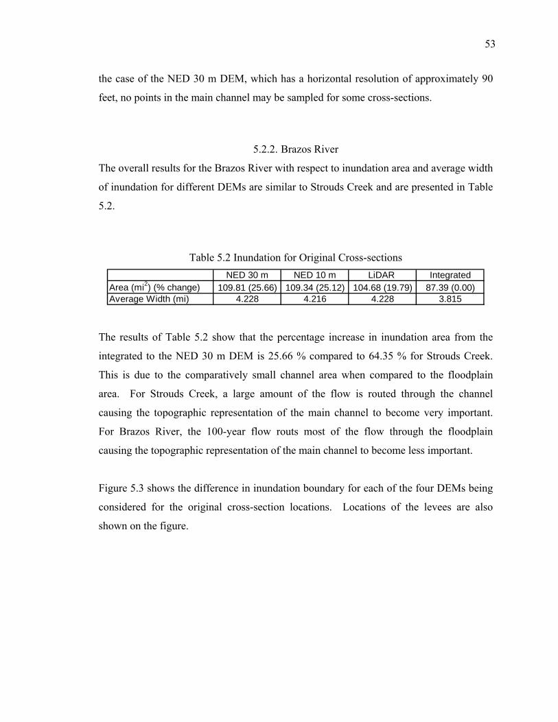
53

the case of the NED 30 m DEM, which has a horizontal resolution of approximately 90

feet, no points in the main channel may be sampled for some cross-sections.

5.2.2. Brazos River

The overall results for the Brazos River with respect to inundation area and average width

of inundation for different DEMs are similar to Strouds Creek and are presented in Table

5.2.

Table 5.2 Inundation for Original Cross-sections NED 30 m NED 10 m LiDAR Integrated

Area (mi2) (% change) 109.81 (25.66) 109.34 (25.12) 104.68 (19.79) 87.39 (0.00)Average Width (mi) 4.228 4.216 4.228 3.815

The results of Table 5.2 show that the percentage increase in inundation area from the

integrated to the NED 30 m DEM is 25.66 % compared to 64.35 % for Strouds Creek.

This is due to the comparatively small channel area when compared to the floodplain

area. For Strouds Creek, a large amount of the flow is routed through the channel

causing the topographic representation of the main channel to become very important.

For Brazos River, the 100-year flow routs most of the flow through the floodplain

causing the topographic representation of the main channel to become less important.

Figure 5.3 shows the difference in inundation boundary for each of the four DEMs being

considered for the original cross-section locations. Locations of the levees are also

shown on the figure.

54

LegendIntegreated

LiDAR

NED 10 m

NED 30 m

Figure 5.3 Inundation Boundary for a) Entire Reach; b) Magnified to the Levees

The section of the Brazos River shown in Figure 5.3 is a downstream section of the river

in which the levees are shown to block flow into the floodplains for the higher resolution

DEMs while the lower resolution DEMs show levee overtopping and flow being routed

into the floodplains. There is also a noticeable difference in the inundation extent

upstream of the section shown in Figure 5.3 between the integrated and LiDAR DEMs in

which the LiDAR DEM shows overtopping of some levees resulting in a larger

inundation area. The difference in inundation over the entire length of the reach being

considered between the integrated and LiDAR DEMs is presented in Figure 5.4.

a)

b)

55

LegendIntegrated

LiDAR

Figure 5.4 Inundation Boundary for Original Cross-sections for the Integrated and

LiDAR DEMs

The change in representation of the main channel causing levee overtopping at some

locations can be seen through a representative HEC-RAS cross-section station 143373.8

feet for both the integrated and LiDAR DEMs in Figure 5.5. The main channel invert for

the integrated DEM cross-section is approximately 25 feet while the main channel invert

for the LiDAR DEM cross-section is approximately 50 feet. The difference in inundation

extent can be seen in the fact that the water surface elevation for the LiDAR DEM cross-

section is 84.53 feet while the integrated DEM cross-section shows a water surface

elevation of 81.72 feet. The difference in water surface elevations is enough to cause

overtopping of the levees at some locations.

56

0 2000 4000 6000 800020

30

40

50

60

70

80

90

100

Station (ft)

Ele

vatio

n (ft

)

Legend

WS 100yr

Ground

Bank Sta

0 2000 4000 6000 800050

60

70

80

90

100

Station (ft)

Ele

vatio

n (ft

)

Legend

WS 100yr

Ground

Bank Sta

Figure 5.5 Cross-section Station 143373.8 for a) Integrated; b) LiDAR DEM

5.3. Effect of Geometry on one-dimensional hydraulic model


using 18 HEC-RAS cross-sectional modifications for Strouds Creek and 12 cross-

sectional modifications for the Brazos River as discussed in sections 4.2.1 and 4.2.2. The

extent of inundation is measured by the area of inundation and the average width of

inundation along the original cross-sections.


Table 5.3 provides the area extent of inundation for each of the 18 cross-sectional

configurations. The percent change in inundation area is shown in parenthesis. The

percent change in inundation area is in reference to the original cross-sectional

configuration for each DEM.

a) b)

57

Table 5.3 Inundation Area (mi2) (% Change) NED 30 m NED 10 m LiDAR Integrated

S 0.199 (0.00) 0.178 (0.00) 0.145 (0.00) 0.121 (0.00)SA1 0.203 (1.73) 0.178 (0.26) 0.154 (5.82) 0.129 (6.19)SA2 0.203 (2.08) 0.179 (0.55) 0.158 (8.54) 0.132 (9.36)SA3 0.201 (1.04) 0.179 (0.92) 0.156 (7.64) 0.131 (8.44)SR1 0.197 (-1.21) 0.174 (-1.82) 0.132 (-8.99) 0.110 (-9.52)SR2 0.187 (-5.88) 0.168 (-5.28) 0.118 (-18.59) 0.098 (-19.15)SR3 0.198 (-0.69) 0.177 (-0.55) 0.131 (-9.86) 0.111 (-8.27)SR4 0.199 (0.00) 0.178 (-0.02) 0.145 (0.07) 0.121 (-0.33)SR5 0.199 (0.00) 0.178 (-0.07) 0.145 (-0.11) 0.121 (-0.08)SR6 0.197 (-1.04) 0.177 (-0.22) 0.144 (-0.58) 0.119 (-1.42)SR7 0.198 (-0.52) 0.177 (-0.11) 0.143 (1.62) 0.120 (-1.17)SR8 0.199 (0.00) 0.177 (-0.20) 0.145 (0.09) 0.121 (-0.08)SR9 0.198 (-0.69) 0.177 (-0.15) 0.143 (-1.39) 0.120 (-1.26)SR10 0.199 (0.00) 0.178 (0.26) 0.142 (-1.97) 0.118 (-2.34)SR11 0.199 (0.00) 0.178 (0.00) 0.144 (-1.07) 0.12 (-1.27)SI1 0.203 (2.08) 0.180 (1.14) 0.157 (7.81) 0.132 (8.85)SI2 0.199 (0.17) 0.179 (0.66) 0.149 (2.75) 0.124 (2.04)SI3 0.193 (-3.11) 0.177 (-0.29) 0.136 (-6.39) 0.112 (-7.86)

From Table 5.3, it is seen that the integrated DEM produced the least area of inundation

for each of the cross-section modifications, followed by the LiDAR DEM, the NED 10 m

DEM, and the NED 30 m DEM. It is also seen that the cross-sectional modifications

where cross-sections are added (SA1, SA2, SA3, SI1) produce the largest area of

inundation, while the least area of inundation is produced from the cross-sectional

modifications where cross-sections are removed (SR1, SR2, SI3). The exception to this

rule is seen in the SR3 modification for the integrated and LiDAR DEMs. For this

modification, the cross-sections on either side of a culvert are removed. The lesser area

shown in Table 5.3 for the SR3 modification is caused by the model producing no

inundation area upstream of the culvert. This result shows the importance of including

cross-sections on either side of a hydraulic structure in one-dimensional hydraulic

modeling.

The results of Table 5.3 also suggest that increasing or decreasing the number of cross-

sections for a high resolution DEM has a larger affect than increasing or decreasing the

number of cross-sections for a lower resolution DEM. The SR2 cross-sectional

58

modification can be used as an example. For both the NED 30 m and NED 10 m DEMs,

the percent decrease in inundation area is below 6%, while the percent decrease in

inundation area for the LiDAR and integrated DEMs is nearly 20%. Figure 5.6 and

Figure 5.7 show the effect of increasing or decreasing the number of cross-sections on the

resulting floodplain for the integrated DEM and NED 30 m DEM, respectively By

adding cross-sections, as is done in the SA1 cross-sectional modification, the area shown

not to be flooded in for the integrated DEM is now flooded in Figure 5.6. By reducing

the number of cross-sections, as is done in the SR1 and SR2 cross-sectional

modifications, the floodplain becomes further degraded. Figure 5.7 shows only a small

change in the inundation area for the NED 30 m DEM when the cross-sectional

configuration is altered. The results of the LiDAR DEM simulations are similar to those

of the integrated DEM while the results of the NED 10 m DEM simulations are similar to

those of the NED 30 m DEM.

59

LegendS

SA1

SR1

SR2

Figure 5.6 Inundation Boundary for the Integrated DEM for a) Entire Reach; b)

Magnified Section for Four Cross-Sectional Modifications

a)

b)

60

LegendS

SA1

SR1

SR2

Figure 5.7 Inundation Boundary for the NED 30 m DEM for a) Entire Reach; b)


To further show the effect of cross-sectional modifications in a one-dimensional HEC-

RAS simulation, Table 5.4 presents the average width of inundation along the original 55

cross-sections for each DEM being evaluated. The results of this table show that

decreasing the number of cross-sections will decrease the average width of inundation

while increasing the number of cross-sections will increase the average width of

inundation. For each of the DEMs being considered, the least average width of

inundation is produced by a cross-sectional configuration in which a significant number

of cross-sections are removed. Conversely, the maximum average width of inundation is

produced by a cross-sectional modification in which a significant number of cross-

a)

b)

61

sections are added. The results of Table 5.4 correspond well to the results of Table 5.3 in

which the areas of inundation for each cross-sectional modification are presented.

Table 5.4 Average Width of Inundation (ft) NED 30 m NED 10 m LiDAR Integrated

S 297.33 264.29 234.40 185.46SA1 301.75 262.31 234.00 184.89SA2 300.58 263.42 235.62 190.39SA3 299.44 263.83 234.12 186.15SR1 297.62 263.79 217.47 171.75SR2 278.76 262.86 200.42 156.99SR3 289.27 258.81 205.78 167.03SR4 297.33 264.29 234.40 184.68SR5 297.33 264.29 232.89 184.68SR6 295.79 264.29 233.22 183.89SR7 297.33 264.84 231.04 182.96SR8 297.33 263.63 234.81 184.60SR9 295.54 264.29 232.29 183.62SR10 297.33 264.79 229.91 180.62SR11 297.33 264.29 233.18 183.01SI1 295.62 264.95 246.56 193.34SI2 293.89 265.36 237.32 186.13SI3 281.44 261.83 227.00 175.68

By removing one or a series of cross sections from the original cross-sectional

configuration, as is done in cross-sectional modifications SR4 to SR11, the width of

inundation only changes in the immediate vicinity of the cross-sections(s) being removed.

For the higher resolution DEMs, removing one cross-section results in a maximum

decrease in inundation width equal to 100 %, meaning the width of inundation is zero

along the cross-section removed. Removing cross-sections(s) at bend in the river results

in the largest change in inundation width although no change in inundation is seen

sufficiently far up or downstream. Cross-sectional modification SR10 removes three

consecutive cross-sections on a relatively straight portion of the river but results in less

change in inundation width than removing one cross-section located on a bend. For the

lower resolution DEMs, the maximum decrease in inundation width due to removing one

or a series of cross-sections is 42 %.

62

5.3.2. Brazos River

The results of the effect of change in cross-section configuration for the Brazos River are

presented in Table 5.5 for each DEM.


B 109.81 (0.00) 109.34 (0.00) 104.68 (0.00) 87.39 (0.00)BA1 109.00 (-0.74) 108.02 (-1.20) 104.04 (-0.61) 90.84 (3.95)BA2 108.67 (-1.04) 107.92 (-1.29) 99.89 (-4.57) 85.65 (-1.99)BA3 108.67 (-1.04) 108.23 (-1.01) 103.15 (-1.46) 86.03 (-1.55)BR1 107.01 (-2.55) 106.74 (-2.37) 104.82 (0.13) 86.16 (-1.41)BR2 103.80 (-5.48) 103.9 (-4.96) 97.17 (-7.18) 83.78 (-4.13)BR3 109.72 (-0.08) 109.23 (-0.10) 104.68 (0.00) 87.24 (-0.17)BR4 109.72 (-0.09) 109.28 (-0.06) 104.70 (0.02) 86.86 (-0.61)BR5 109.65 (-0.15) 109.15 (-0.17) 104.53 (-0.14) 86.91 (-0.54)BR6 110.67 (0.78) 110.24 (0.82) 105.96 (1.22) 87.83 (0.51)BR7 109.61 (-0.18) 109.11 (-0.21) 105.79 (1.06) 87.04 (-0.39)BR8 109.16 (-0.60) 108.48 (-0.78) 105.71 (0.99) 88.60 (1.39)

From Table 5.5, it is seen that the integrated DEM produced the least area of inundation

for each of the cross-sectional modifications, followed by the LiDAR DEM, the NED 10

m DEM, and the NED 30 m DEM, which is similar to the results seen in Strouds Creek.

This table also shows that the largest inundated area for the integrated DEM is produced

by the BA1 cross-sectional modification, while the largest inundated area for the other

three DEMs is produced for the BR6 modification. When cross-section placement is

changed in the vicinity of levees, a large change in inundation area is seen. This large

change is due to the process by which HEC-GeoRAS linearly interpolates the floodplain

boundary between adjacent cross-sections. For the Brazos River reach being analyzed,

the levees generally run parallel to the river before branching off perpendicular, making a

modified “U” shape as is seen in Figure 5.3. If a cross-section is removed from the

section of levee parallel to the river, the resulting floodplain area will generally increase

because the boundary will be linearly interpolated from a cross-section upstream of the

levee to the cross-section just downstream of any cross-section being removed. In

reality, the floodplain boundary should follow the levee border, but because of the linear

63

interpolation process between cross-sections, the HEC-GeoRAS boundary is not the same

as the levee boundary. If a cross-section is removed upstream/downstream of the

upstream/downstream perpendicular section of the levee, the floodplain area will either

increase or decrease depending on the width of inundation along the cross-section just

upstream/downstream of any cross-sections removed. Figure 5.8 and Figure 5.9 present a

section of the floodplain located near a levee with four cross-sectional modifications for

the integrated DEM and NED 30 m DEM, respectively.

LegendB

BA1

BR1

BR2



a)

b)

64

For the integrated DEM, changing the cross-sectional configuration near levees is shown

to cause large changes in the floodplain. For modification BA1, a cross-section is added

just upstream of the perpendicular section of the levee causing an increase in the

inundation area. For modifications BR1, cross-sections are removed from the section of

levee running parallel to the river causing an increase in inundation area at this section.

For modification BR2, cross-sections are removed both upstream of the perpendicular

section of the levee and along the parallel section of the levee causing the floodplain area

to be substantially reduced at this location.

LegendB

BA1

BR1

BR2



a)

b)

65

For the lower resolution DEMs, changing the cross-sectional configuration in the vicinity

of the levees causes little change because each cross-sectional modification shows levee

overtopping. Changing the cross-sectional modification for the lower resolution DEMs

generally results in a decrease in the inundation extent.

Table 5.6 presents the average width of inundation for each of the four DEMs for each

cross-sectional modification. For the integrated DEM, inundation extent is complex near

levee locations, and may cause an increase or decrease in the average width of inundation

depending on the configuration of the cross-section locations. For the lower resolution

DEMs, when cross-sections are added on bends in the river, the inundation extent

increases, and when cross-sections are removed from bends in the river, inundation extent

decreases. For cross-sections located on straight reaches of the river, removing a cross-

section generally results in a decrease in inundation length along that cross-section.

Table 5.6 Average Width of Inundation (mi) NED 30 m NED 10 m LiDAR Integrated

B 4.23 4.22 4.23 3.82BA1 4.19 4.21 4.20 3.76BA2 4.26 4.24 4.13 3.62BA3 4.23 4.21 4.23 3.79BR1 4.14 4.13 4.18 3.69BR2 4.04 4.05 4.15 3.67BR3 4.23 4.21 4.23 3.81BR4 4.22 4.21 4.21 3.80BR5 4.20 4.21 4.22 3.78BR6 4.25 4.23 4.18 3.83BR7 4.22 4.21 4.22 3.81BR8 4.23 4.20 4.25 3.84

By removing one or a series of cross-sections from the higher resolution DEMS, the

maximum increase in inundation width is 25 % while the maximum decrease is 22%.

For the lower resolution DEMs, a maximum change in average width of inundation is 7

% when one or a series of cross-sections are removed. Similar to the results from Strouds

66

Creek, cross-sectional modifications alter the floodplain more for higher resolution

DEMs.

5.4. Effect of Topography on the two-dimensional hydraulic model


using the 10 foot mesh resolution for Strouds Creek and the 125 foot mesh resolution for

the Brazos River. The extent of inundation is measured by the area of inundation and the

average width of inundation along the cross-sections.


Table 5.7 presents the area of inundation as well as the average width of inundation and

the percent change in inundation area using the integrated DEM as the benchmark for

each of the four DEMs being evaluated for the 10 foot mesh resolution.

Table 5.7 Inundation for the 10 ft mesh resolution NED 30 m NED 10 m LiDAR Integrated

Area (mi2) (% change) 0.153 (17.44) 0.150 (15.70) 0.143 (10.53) 0.130 (0.00)Average Width (ft) 274.97 268.23 250.78 224.13

Table 5.7 shows that increasing the DEM resolution produces the least inundation area.

The integrated DEM produces the least extent of inundation area, followed by the

LiDAR, NED 10m, and NED 30m DEMs. The area of inundation for the NED 30 m

DEM is approximately 17% larger than that of the integrated DEM. The results for

average width of inundation in Table 5.7 also show increasing inundation as the

resolution of the DEM decreases. The average width of inundation increases from 224 to

275 feet from the integrated to the NED 30 m DEM. Figure 5.10 presents the floodplain

for a section of Strouds Creek developed using FESWMS at a 10 foot mesh resolution for

each DEM.

67

LegendIntegrated

LiDAR

NED 10 m

NED 30 m

Figure 5.10 Inundation Boundary for a) Entire Reach; b) Magnified to a Bend in the

River for the FESWMS 10 foot mesh resolution.

For each floodplain boundary shown in Figure 5.10, there is a slight increase in

inundation area as the resolution of the DEM is decreased. There is also a shift in the

representation of the floodplain between the higher and lower resolution DEMs. This

figure shows the boundary of the integrated and LiDAR DEMs to be nearly identical,

while there is a slight shift in the floodplain boundary for the NED 10 m DEM and a clear

shift in the floodplain boundary for the NED 30 m DEM.

a)

b)

68

5.4.2. Brazos River

The results of effect of topographic representation for the two-dimensional model are

shown in Table 5.8 for the 125 foot mesh resolution.

Table 5.8 Inundation for the 125 ft mesh resolution

NED 30 m NED 10 m LiDAR IntegratedArea (mi2) (% change) 16.84 (7.62) 16.57 (5.95) 16.64 (6.35) 15.64 (0.00)

Average Width (mi) 3.24 3.24 3.28 2.98

Similar to the results from Strouds Creek, as the resolution of the DEM decreases, the

inundation area increases. The maximum increase in inundation area for the Brazos

River is below 8 %, while maximum increase in inundation area for Strouds Creek is

above 17%. The Brazos River is affected less by changes in DEM because the

representation of the main channel becomes less important for higher flows. Both the

average width and inundation area are similar for the NED 30 m, NED 10 m, and LiDAR

DEMs. Figure 5.11 presents the floodplain for a section of the Brazos River developed

using FESWMS at a 125 foot main channel mesh resolution mesh resolution for each of

the four DEMs being considered.

69

LegendIntegrated

LiDAR

NED 10 m

NED 30 m

Figure 5.11 Inundation Boundary for 125 ft Mesh Resolution for a) Entire Reach; b)

Upstream Section

Figure 5.11 shows the upstream, 9 mile reach of the Brazos River for four different

DEMs. The images show that the inundation extent is similar for each of the four DEMs

being considered, although the integrated DEM boundary shows slightly less inundation

on the northern side of the river. For each of the four DEMs being analyzed, the flow

does not extend to the floodplain on the southern side of the river because the main

channel is steep and extends to a higher elevation on that side. Figure 5.12 shows cross-

section station 206697.9 feet for the integrated DEM. This figure shows the large bank

on the southern side of the Brazos River preventing flow into this floodplain on the nine

mile upstream section being modeled in FESWMS.

a)

b)

70

0 5000 10000 15000 20000 2500040

50

60

70

80

90

100

110

120

Station (ft)

Ele

vatio

n (ft

)Legend

WS 100yr

Ground

Bank Sta

Figure 5.12 Cross-section showing large bank on south side of the Brazos River

5.5. Effect of Geometry on two-dimensional hydraulic model


using 2 mesh resolutions for Strouds Creek and 2 mesh resolutions for the Brazos River.

The extent of inundation is measured by the area of inundation and the average width of



Table 5.9 presents the area of inundation as well as the percent change in inundation area

using the 10 foot mesh resolution as the benchmark for four DEMs and for two mesh

resolutions.


10-ft Mesh Resolution 0.153 (0.00) 0.150 (0.00) 0.143 (0.00) 0.130 (0.00)20-ft Mesh Resolution 0.151 (-1.00) 0.144 (-3.92) 0.137 (-4.22) 0.127 (-2.58)

71

The results of Table 5.9 show that the 20 foot mesh resolution produces a smaller area of

inundation for each of the four DEMs, although the maximum decrease in inundation

area from the 10 foot to the 20 foot mesh resolution is below 5 %. To further show how

mesh resolution changes the extent of inundation, Table 5.10 presents the average width

of inundation for each of the four DEMs for two mesh resolutions.


10-ft Mesh Resolution 274.97 268.23 250.78 224.1320-ft Mesh Resolution 269.88 256.19 239.48 221.00

Similar to the results of Table 5.9, the results of this table suggest that the 10 foot mesh

resolution produces a larger inundation extent than that of the 20 foot mesh resolution for

Strouds Creek, although the change in average width never exceeds 5 %.

5.5.2. Brazos River

The results for the effect of mesh resolution on the inundation extent are presented in

Table 5.11 The percent change is in reference to the 125 foot mesh resolution.

Table 5.11 Inundation Area (mi2) (% Change)

Contrary to the results for Strouds Creek where the higher resolution mesh produces the

larger inundation area, the lower resolution mesh produces a larger inundation area for

three of the four DEMs. Similar to the results from Strouds Creek, the change in

inundated area from one mesh resolution to another is small and never exceeds 2.5 %.

NED 30 m NED 10 m LiDAR IntegratedFESWMS 125-ft Resolution 16.84 (0.00) 16.57 (0.00) 16.64 (0.00) 15.64 (0.00)FESWMS 250-ft Resolution 16.81 (-0.16) 16.94 (2.21) 17.02 (2.30) 15.85 (1.29)

72

The only DEM to predict more inundation area for the 250 foot main channel mesh

resolution is the NED 30 m DEM. Table 5.12 provides further information as to the

extent of inundation for differing mesh resolutions. The average width of inundation for

each DEM is very similar between the 125 foot and 250 foot main channel mesh

resolutions. The largest change is seen in the LiDAR DEM where the average width

increases by over 6 % from the 125 to the 250 foot main channel mesh resolution.

Table 5.12 Average Width of Inundation (mi) NED 30 m NED 10 m LiDAR Integrated

FESWMS 125-ft Resolution 3.24 3.24 3.28 2.98FESWMS 250-ft Resolution 3.19 3.28 3.49 3.05

5.6. Comparison of HEC-RAS and FESWMS

In this section, the one-dimensional model HEC-RAS and the two-dimensional model

FESWMS are compared for hydraulic modeling and flood inundation mapping. For both

FESWMS and HEC-RAS, changes in topography and geometry are considered. The

extent of inundation is measured by the area of inundation and the average width of



Table 5.13 presents the inundation area for each of the HEC-RAS cross-sectional

modification (except those where only one or a series of cross-sections were removed)

and for both FESWMS mesh resolutions for each of the four DEMs. To compare the

results of the HEC-RAS simulations with those of the FESWMS simulations, all HEC-

RAS inundation boundary polygons are clipped to the same length as those developed

using FESWMS.

73

Table 5.13 Inundation Area (mi2)

NED 30 m NED 10 m LiDAR IntegratedS 0.171 0.155 0.128 0.109

SA1 0.173 0.156 0.134 0.115SA2 0.174 0.156 0.138 0.119SA3 0.173 0.156 0.137 0.117SR1 0.171 0.153 0.116 0.100SR2 0.168 0.152 0.107 0.091SI1 0.175 0.157 0.136 0.118SI2 0.171 0.156 0.130 0.111SI3 0.170 0.157 0.123 0.103

10-ft 0.153 0.150 0.143 0.13020-ft 0.151 0.144 0.137 0.127

Area of Inundation (mi2)

From Table 5.13, it is seen that the inundated area for the HEC-RAS analysis is larger

than the inundated area for the FESWMS analysis for the lower resolution DEMs and

smaller than the inundated area for the FESWMS analysis for the higher resolution

DEMs. These results also suggest that HEC-RAS is more susceptible to a change in

DEM than FESWMS as the increase in area from the high resolution DEMs to the high

resolution DEMs is larger for HEC-RAS. For the HEC-RAS simulations, the area

increases by around 0.6 mi2 for some cross-sectional modifications while the area

increases by approximately 0.2 mi2 for the FESWMS simulations.

The results of Table 5.13 also show that the LiDAR and NED 10 m DEMs most closely

predict the inundation area between HEC-RAS and FESWMS while the integrated and

NED 30 m DEMs produce inundation area results very different between HEC-RAS and

FESWMS. Figure 5.13 shows the floodplain developed from the FESWMS 10 foot mesh

resolution along with the floodplain developed using four HEC-RAS cross-sectional

configurations for the integrated DEM. In this figure, the floodplain produced in HEC-

RAS for the original cross-sections shows discontinuities in the floodplain which are not

seen in the FESWMS floodplain. The SA1 modification shows a floodplain more similar

to the FESWMS simulation. The SR1 and SR2 modifications show results very different

than the results of the FESWMS simulation as the floodplain becomes degraded when

74

cross-sections are removed. This figure as well as the results of Table 5.13 suggest that,

for the higher resolution DEMs, the results from the HEC-RAS simulations become more

similar to the results of the FESWMS simulations when cross-sections are added.

Although increasing the number of HEC-RAS cross-sections produces an area more

similar to FESWMS simulation results, each HEC-RAS simulation resulted in an area

less than any FESWMS simulation for the integrated DEM.

Figure 5.13 Inundation Boundary for 10 ft Mesh Resolution and a) S; b) SA1; c) SR1; d)

SR2 for the Integrated DEM

Figure 5.14 shows the floodplain developed from the FESWMS 10 foot mesh resolution

along with the floodplain developed using four HEC-RAS cross-sectional configurations

for the NED 30 m DEM. Because the original HEC-RAS cross-sectional modification

overestimated the FESWMS simulated area, reducing the number of HEC-RAS cross-

sections produces an area more similar to that of the FESWMS simulations. It should be

noted that although reducing the number of cross-sections in HEC-RAS produces an area

more similar to that of the FESWMS simulations, each HEC-RAS simulation predicted

an area larger than any FESWMS simulation for the lower resolution DEMs.

a)

c) d)

b)

75

Figure 5.14 Inundation Boundary for 10 ft Mesh Resolution and a) S; b) SA1; c) SR1; d)

SR2 for the NED 30 m DEM

To further show that the HEC-RAS simulations for the high resolution DEMs predict

larger inundation extents than those of FESWMS and for the lower resolution predict

smaller inundation extents than those of FESWMS, Table 5.14 presents the average width

of inundation along the original cross-sections for each FESWMS and HEC-RAS

simulation. Conclusions from this table coincide with those presented in Table 5.13.


S 311.57 281.30 249.13 203.33SA1 310.71 278.90 249.56 202.62SA2 309.25 280.30 251.04 207.98SA3 314.21 280.04 248.78 203.72SR1 313.86 282.41 229.22 189.15SR2 305.50 285.58 215.97 174.23SI1 311.86 280.68 255.15 211.71SI2 310.66 280.40 247.81 206.78SI3 304.05 282.67 241.22 196.89

10-ft 274.97 268.23 250.78 224.1320-ft 269.88 256.19 239.48 221.00

a) b)

c) d)

76

5.6.2. Brazos River

The results comparing the inundation area from the HEC-RAS analysis with the

FESWMS analysis for the Brazos River are presented in Table 5.15.

Table 5.15 Inundation Area (mi2)

NED 30 m NED 10 m LiDAR IntegratedB 16.43 16.43 16.42 13.00BA1 16.13 15.93 16.46 13.69BA2 16.00 15.84 16.39 13.44BA3 16.16 16.17 16.43 13.48BR1 16.29 16.20 16.53 12.27BR2 12.73 12.66 12.90 10.57

125-ft 16.84 16.57 16.64 15.64150-ft 16.81 16.94 17.02 15.85

Area of Inundation (mi2)

The results of Table 5.15 show that the inundated area from FESWMS is always larger

than that of HEC-RAS. For the integrated DEM, the inundated area produced in

FESWMS is substantially larger than the inundated area produced in HEC-RAS. For the

other three DEMs being analyzed, the inundated areas produced from FESWMS and

HEC-RAS are more similar. For the NED 10 m and LiDAR DEMs, the FESWMS 125

foot mesh resolution and most HEC-RAS cross-sectional modifications produce similar

results. The FESWMS simulations for the NED 30m DEM predict an area larger than

any area predicted using a HEC-RAS simulation.

Similar to the results from Strouds Creek, Table 5.15 shows that HEC-RAS is more

susceptible to changes in DEM than is FESWMS. The difference in inundated area from

the FESWMS simulation for the integrated DEM to the lower resolution DEMs is less

than 1.2 mi2. For the HEC-RAS analysis, the difference in inundated area between the

integrated DEM and the lower resolution DEMs is above 3 mi2 for some of the cross-

sectional modifications. This table also shows that by increasing the number of cross-

sections (BA1, BA2, and BA3) for analysis of the integrated DEM the inundated area

77

becomes closer to the inundated area predicted by FESWMS. For the two lower

resolution DEMs and the LiDAR DEM, all cross-sectional modifications produce similar

floodplain areas to the FEWSMS floodplain area with the exception of the one-third

cross-sectional modification. The one-third cross-sectional modification produces an

area much less than any other modification due to much of the area being cut off when

the floodplain boundary is interpolated between cross-sections.

Figure 5.15 and Figure 5.16 present the inundation boundaries for the FESWMS 125 foot

main channel mesh resolutions and four HEC-RAS cross-sectional modifications for the

integrated and NED 30 m DEMs, respectively.

Figure 5.15 Inundation Boundary for 125 ft Mesh Resolution and a) S; b) SA1; c) SR1;

d) SR2 for the Integrated DEM

Similar to what is seen for Strouds Creek, increasing the number of HEC-RAS cross-

sections when using the integrated DEM produces an area more similar to that of

FESWMS, although FESWMS produces a continuous floodplain while HEC-RAS

produces discontinuous floodplain. This is due to the process by which HEC-GeoRAS

a)

c) d)

b)

78

subtracts the topographic data from the water surface elevations to determine the

floodplain.

Figure 5.16 Inundation Boundary for 125 ft Mesh Resolution and a) S; b) SA1; c) SR1;

d) SR2 for the NED 30 m DEM

Figure 5.16 shows that the floodplain extent for the original cross-sectional configuration

and modifications BA1 and BR1 are similar and that the floodplain boundary from the

FESWMS simulation is greater than any HEC-RAS boundary. Contrary to what is seen

in the results for Strouds Creek, the BR2 modification causes a large change in

inundation extent for the lower resolution DEMs.

a)

c) d)

b)

79

CHAPTER 6. SUMMARY AND CONCLUSIONS

6.1. Effect of topography on 1D and 2D hydraulic models

The first objective of this research is to evaluate the effect of topography on both a one-

and a two-dimensional hydrodynamic model. This is accomplished by using four DEMs;

integrated, LiDAR, NED 10m, and NED 30 m to produce floodplain maps using HEC-

RAS and FESWMS for Strouds Creek in North Carolina and the Brazos River in Texas.

For both river reaches evaluated, both the area of inundation and average width of

inundation along the original cross-sections increase as the resolution of the DEM

decreases. For Strouds Creek, the NED 30 m DEM produces an area 65 % larger than

that of the integrated DEM, while for the Brazos River, the NED 30 m DEM produces an

area approximately 26 % larger than that of the integrated DEM using HEC-RAS. The

average width of inundation increases by over 60 % for Strouds Creek and by

approximately 11 % for the Brazos River from the integrated DEM to the NED 30 m

DEM.

From the two-dimensional floodplain mapping process, the inundation area for Strouds

Creek for the NED 30 m DEM is 17 % larger than the inundation area for the integrated

DEM, and for the Brazos River, the inundation area for the NED 30 m DEM is 8 % larger

than that of the integrated DEM. The average width of inundation increases by nearly 23

% for Strouds Creek and by nearly 9 % for the Brazos River from the integrated DEM to

the NED 30 m DEM.

The reason for a larger change between the low and high resolution DEMs for Strouds

Creek is that the 100-year flow is a relatively small value causing most of the water to be

routed through the main channel. When most of the flow is routed through the main

80

channel, the main channel topographic representation becomes very important. For the

Brazos River, with a high flow rate, most of the flow is routed through the floodplains

making the topographic representation of the main channel less important.

Results from this thesis are similar to those found in other studies that decreasing

resolution of the topographic data causes an increase in the floodplain area. In studies

performed by Sanders (2007) and Casas et al. (2007) it was found that increasing the

resolution of the DEM leads to a decrease in inundated area.

6.2. Effect of geometry on 1D and 2D hydraulic models

The second topic addressed in this thesis is the effect of geometry on one- and two-

dimensional hydraulic models. For the one-dimensional HEC-RAS model, 18 cross-

sectional configurations are analyzed for Strouds Creek and 12 cross-sectional

configurations are analyzed for the Brazos River. For Strouds Creek, increasing the

number of cross-sections generally results in an increase in the inundation extent. For the

Brazos River, the same trend is seen that increasing the number of cross-sections

increases the inundation extent for the higher resolution DEMs except in the vicinity of

the levees. Changing the cross-sectional configuration near levees produces complex

results and produces significant changes in both inundation area and width of inundation

along the cross-sections. Removing specific cross-sections generally results in a decrease

in width of inundation along the cross-section removed for both river reaches analyzed

except when the cross-section being removed is located near a levee. Cross-sections

sufficiently far up or downstream are unaffected by a single or consecutive cross-sections

being removed. Cross-section modifications are shown to alter results for higher

resolution DEMs more than for lower resolution DEMs. Similar to the results found in a

study by Samuels (1990), cross-sectional configuration is important in hydraulic

modeling and floodplain mapping.

81

For the two-dimensional FESWMS model, two mesh resolutions are tested for both

Strouds Creek and the Brazos River. For Strouds Creek, the 10 foot mesh resolution

produces a larger inundation area than the 20 foot mesh resolution for each of the four

DEMs being analyzed. The maximum change in inundation area between the two mesh

resolutions for Strouds Creek is less than 5 %. For the Brazos River, the 250 foot mesh

resolution is shown to produce a larger inundation area than the 125 foot mesh resolution

for three of the four DEMs analyzed, although by a maximum value of only 2.3 %. In a

study performed by Hardy et al. (1998), it was found that increasing the mesh resolution

results in a decrease in inundation area similar to what was found in this thesis for the

Brazos River. A study by Horritt et al. (2006) suggests that two-dimensional models are

sensitive to changes in mesh resolution.

6.3. Comparison of 1D and 2D Hydraulic Models

The final objective of this thesis is to compare the results from HEC-RAS and FESWMS

in flood inundation mapping. The 18 cross-sectional configurations for Strouds Creek

and 12 cross-sectional configurations for the Brazos River are compared to the two mesh

resolutions for each river reach using four DEMs. It is found that the HEC-RAS model is

more susceptible to changes in DEM than the FESWMS model. For Strouds Creek, the

percent change in inundation area from the integrated DEM to the NED 30 m DEM for

the HEC-RAS simulations is approximately 57 % and for the FESWMS simulations is 18

%. For the Brazos River, the percent change in inundation area from the lower resolution

DEMs to the high resolution DEMs is 26 % for the HEC-RAS simulations and 8 % for

the FESWMS simulations.

For the higher resolution DEMs, LiDAR and integrated for Strouds Creek and integrated

for the Brazos River, FESWMS predicts a larger area than HEC-RAS. For the lower

resolutions DEMs for Strouds Creek, HEC-RAS predicts a larger inundation area, and the

three remaining DEMs for the Brazos River predict approximately equal areas using both

HEC-RAS and FESWMS. For the higher resolution DEMs, the HEC-RAS area becomes

82

more similar to that of FESWMS when cross-sections are added to the simulations. For

Strouds Creek using the lower resolution DEMs, the results from HEC-RAS and

FESWMS become more similar when cross-sections are removed. Changing mesh

resolution or cross-sectional configuration is found to have less of an affect on the

resulting floodplain than changes in the DEM. Results from this thesis are similar to that

of other studies in which the results from one- and two-dimensional models are found to

produce different floodplain areas (Juza and Barad, 2000, Schumann et al., 2007).

The one-dimensional HEC-RAS model linearly interpolates the floodplain boundary

between cross-sections, and then defines the floodplain by subtracting the topographic

data from the water surface elevations. This process often results in a discontinuous

floodplain. The advantage of using the one-dimensional floodplain mapping process is

that is easy to use and produces results quickly. In a HEC-RAS simulation, the

Manning’s n value is often used as the lone calibrating parameter, and can change results

significantly (HEC, 2002). Where the HEC-RAS simulation takes a matter of seconds to

complete, the FESWMS simulation can take multiple hours. The advantage of the two-

dimensional model is that it produces a continuous floodplain as it represents the

topography as a series of mesh elements and can model flow in both the lateral and

longitudinal directions resulting in a more accurate representation of the floodplain. For

a FESWMS simulation, two calibrating parameters, Manning’s n and eddy viscosity, can

be used as calibrating parameters and may have an affect of the results of the hydraulic

simulations (FESWMS, 2002). The experience of the modeler can have an affect on the

resulting floodplain due to the calibrating parameters in both the one- and two-

dimensional model and the meshing type in the two-dimensional model.

6.4. Future Work

Future work on hydraulic modeling and flood inundation mapping using 1D and 2D

models should consider the effect of the calibrating parameters, Manning’s n for HEC-

RAS and both Manning’s n and eddy viscosity for FESWMS. These parameters should

83

be used to calibrate and validate the models to be used and compared against known

historical high water marks or floodplain boundaries.

Future work should also consider a broader range of mesh resolutions in FESWMS as

well as the effect of meshing type. Due to the lack of computing capabilities of the

machine used to perform the FESWMS simulations, very high mesh resolutions could not

be examined. As the computing capabilities are increased, the effect of the levees in

FESWMS should also be examined for the Brazos River.

To further evaluate the effects of topographic data, geometric data, and type of model

used on hydraulic modeling and flood inundation mapping, more study areas should be

evaluated. These study areas should include a broad range of characteristics including

length of the river reach, width of the floodplain, slope, bridges and levees, and land use.

Other one- and two-dimensional models should also be used to compare results.

84

LIST OF REFERENCES

Bates, P.D., and De Roo, A.P.G. A Simple Raster-Based Model for Flood Inundation Simulation. Journal of Hydrology, 236.1-2 (2000): 54-77.

Bates P.D., Marks K.J., Horritt M.S. Optimal use of high-resolution topographic data in flood inundation models. Hydrological Processes 17 (2003): 537- 557.

Bates, P.D., Horritt, M.S., Hunter, N.M., Mason, D., Cobby, D. Numerical modelling of floodplain flow. Computational Fluid Dynamics: Applications in Environmental Hydraulics, 2005 John Wiley & Sons, Ltd. 271 – 297.

Brandt, S.A. Resolution issues of elevation data during inundation modeling of river floods. Proc. XXXI Int. Association of Hydraulic Engineering and Research Congress, Water Engineering for the Future: Choices and Challenges, September 11 – 16 (2005), Seoul, Korea: 3572 – 3581.

Casas A., Benito V.R., Thorndycraft V.R., Rico M. The topographic data source of digital terrain models as a key element in the accuracy of hydraulic flood modelling. Earth Surface Processes and Landforms 31 (2006): 444-456.

Charlton M.E., Large A.R.G., Fuller I.C. Application of airborne LiDAR in river environments: The River Coquet, Northumberland, UK. Earth Surface Processes and Landforms 28 (2003): 299-306.

Cobby D.M., Mason D.C., Davenport I.J. Image processing of airborne scanning laser altimetry for improved river flood modelling. ISPRS Journal of Photogrammetry and Remote Sensing 56 (2001): 121-138.

Crowder, D. W., and P. Diplas. Using Two-Dimensional Hydrodynamic Models at Scales of Ecological Importance. Journal of Hydrology, 230.3-4 (2000): 172-91.

Dutta, D., Alam, J., Umeda, K., Hayashi, M., Hironaka, S. A two-dimensional hydrodynamic model for flood inundation simulation: a case study in the lower Mekong river basin. Hydrologic Processes 21 (9) (2007): 1223 – 1237.

FESWMS FST2DH User’s Manual. Federal Highway Administration. Publication number FHWA-RD-03-053 (2002).

85

Haile, A.T. and Rientjes T.H.M., Effects of LiDAR DEM resolution in flood modelling: a model sensitivity study for the city of Tegucigalpa, Honduras. International Archives of Photogrammetry, Remote Sensing and Spatial Information Sciences 36 (Part 3/W19) (2005): 168–173.

Hardy, R.J., Bates, P.D. and Anderson, M.G. The Importance of Spatial Resolution in Hydraulic Models for Floodplain Environments. Journal of Hydrology, 216.1-2 (1999): 124-36.

HEC-GeoRAS user’s manual available at www.hec.usace.army.mil/software/hec-ras/hec-georas.html.

HEC-RAS hydraulic reference manual available at www.hec.usace.army.mil/ software/hec-ras/hec-georas.html.

HEC-RAS user’s manual available at www.hec.usace.army.mil/software/hec-ras/.

Hodgson, M.E., Jensen, J.R., Schmidt, L., Schill, S., Davis, B. An Evaluation of LIDAR- and IFSAR-Derived Digital Elevation Models in Leaf-on Conditions with USGS Level 1 and Level 2 DEMs. Remote Sensing of Environment, 84.2 (2003): 295-308.

Horritt, M. S., and Bates, P.D. Effects of Spatial Resolution on a Raster Based Model of Flood Flow. Journal of Hydrology, 253.1-4 (2001): 239-49.

Horritt, M.S., and Bates, P.D. Evaluation of 1D and 2D Numerical Models for Predicting River Flood Inundation. Journal of Hydrology, 268.1-4 (2002): 87-99.

Horritt, M.S., P.D. Bates, and M.J. Mattinson. Effects of Mesh Resolution and Topographic Representation in 2D Finite Volume Models of Shallow Water Fluvial Flow. Journal of Hydrology, 329.1-2 (2006): 306-14.

Hunter, N.M., Bates, P.D., Horritt, M.S., Wilson, M.D. Simple Spatially-Distributed Models for Predicting Flood Inundation: A Review. Geomorphology, 90.3-4 (2007): 208-225.

Juza, B., and Barad, M. Dynamic and steady state modeling approaches to riverine hydraulic studies using 1-D, looped 1-D and 2-Dimensional topological discretization. www.engr.ucdavis.edu/~edllab/Users/Barad/Papers/Hydroinformatics2000.pdf.

Kelly, B.P., Rydlund Jr., P.H. Estimated Flood-Inundation Mapping for the Lower Blue River in Kansas City, Missouri. USGS Scientific Investigations Report 2006-5089 (2003-2005).

86

Leopardi A, Oliveri E, Greco M. Two-dimensional modeling of floods to map risk-prone area. Journal of Water Resources Planning and Management (2002): 168-178.

Mason DC, Cobby DM, Horritt MS, Bates PD. Floodplain friction parameterization in two-dimensional river flood models using vegetation heights derived from airborne scanning laser altimetry. Hydrological Processes 17 (2003): 1711-1732.

McMillan, Hilary K., and James Brasington. Reduced Complexity Strategies for Modelling Urban Floodplain Inundation. Geomorphology, 90.3-4 (2007): 226-243.

Merwade, V. Tutorial on using HEC-GeoRAS with ArcGIS 9.1. (2006). http://web.ics.purdue.edu/~vmerwade/education/georastutorial.pdf

Merwade, V., Cook, A., Coonrad, J. GIS techniques for creating river terrain models for hydrodynamic modeling and flood inundation mapping. A possible submission to Environmental Modelling and Software (2007).

Mohammed, T.A., Said, S., Bardaie, M.Z., Basri, S. One-Dimensional Simulation of Flood Levels in a Tropical River System Using HEC-2 Model. Joint International Conference on Computing and Decision Making in Civil and Building Engineering, June 14 – 16 (2006): Montreal, Canada.

Musser, J.W., Dyar T.R. Two-Dimensional Flood-Inundation Model of the Flint River at Albany, Georgia. Proceedings of the 2005 Georgia Water Resources Conference, April 25 – 27 (2005): University of Georgia, Athens, Georgia.

Noman, N.S., Nelson, E.J., Zundel, A.K. Review of automated flood plain delineation from digital terrain models. Journal of Water Resource Planning and Management, 127 (2001): 394-402.

O'Brien, J. S., Julien, P. Y. and Fullerton, W. T. Two-dimensional water flood and mudflow simulation. Journal of the Hydraulics Division, ASCE, 119 (1993): 244-261.

Omer C.R., Nelson E.J., Zundel A.K. Impact of varied data resolution on Hydraulic Modeling and Floodplain Delineation. Journal of the American Water Resources Association 39 (2) (2003): 467- 475.

Papanicolaou, A., Elhakeem, M. Hydraulic performance of shallow water habitat in the Missouri River for ecological studies.. Proceedings of the 7th International Conference on HydroScience and Engineering September 10- 13 (2006): Philadelphia, USA.

Samuels, P.G. Cross-section location in 1-D models. International Conference on River Flood Hydraulics, September 17 – 20 (1990).

87

Sanders, Brett F. Evaluation of on-Line DEMs for Flood Inundation Modeling. Advances in Water Resources, 30.8 (2007): 1831-43.

Schumann, G., Matgen, P., Cutler, M.E.J., Black, A., Hoffman, L., Pfister, L. Comparison of Remotely Sensed Water Stages from LiDAR, Topographic Contours and SRTM. ISPRS Journal of Photogrammetry and Remote Sensing, In Press, Corrected Proof.

Sinnakaudan S, Ab Ghani A, Chang C.K. Flood inundation analysis using HEC-6 and ArcView GIS 3.2a. In Proceeding, 5th International Conference on Hydro-Science & Engineering, September 18–21 (2002), Warsaw University of Technology, Poland.

Smith MJ, Edwards EP, Priestnall G, Bates PD. Exploitation of new data types to create digital surface models for flood inundation modeling, FRMRC Research Report UR3, FRMRC, UK: (2006). www.floodrisk.org.uk.

SMS version 9.2 tutorials. Brigham Young University, Environmental Modeling Research Laboratory (2006).

Tayefi, V., Lane, S.N., Hardy, R.J., Yu, D. A comparison of one- and two-dimensional approaches to modeling flood inundation over complex upland floodplains. Hydrologic Processes 21 (2007): 3190 – 3202.

Wagner, C.R., Mueller, D.S., USGS. Calibration and Validation of a Two-Dimensional Hydrodynamic Model of the Ohio River, Jefferson County, Kentucky. Water Resources Investigations Report 01-4091 (2001).

Werner M, Blazkova S, Petr J. Spatially distributed observations in constraining inundation modelling uncertainties. Hydrological Processes 19 (2005): 3081-3096.

Wilson, M.D., Atkinson, P.M., A comparison of remotely sensed elevation datasets for flood inundation modeling. Proceedings of the 7th International Conference on Geocomputation (2003): University of Southampton, U.K.

Winters, K.E. Simulations of flooding Tchoutacabouffa River at State Highways 15 and 67 at D’lberville, Mississippi.. Water Resources Investigations Report 01-4007 (2000).

Zanichelli, G., Caroni, E., Fiorotto, V. River Bifurcation Analysis by Physical and Numerical Modeling. Journal of Hydraulic Engineering 130 – 3 (2004): 237-242.

comparison of one-dimensional hec-ras with two-dimensional

Documents